\ul \DeclareAcronymBEM short = BEM , long = basis expansion model , short-plural = s , long-plural = s \DeclareAcronymOMP short = OMP , long = orthogonal matching pursuit , short-plural = s , long-plural = s \DeclareAcronymSBL short = SBL , long = sparse Bayesian learning , short-plural = s , long-plural = s
Efficient Off-Grid Bayesian Parameter Estimation for Kronecker-Structured Signals
Abstract
This work studies the problem of jointly estimating unknown parameters from Kronecker-structured multidimensional signals, which arises in applications like intelligent reflecting surface (IRS)-aided channel estimation. Exploiting the Kronecker structure, we decompose the estimation problem into smaller, independent subproblems across each dimension. Each subproblem is posed as a sparse recovery problem using basis expansion and solved using a novel off-grid sparse Bayesian learning (SBL)-based algorithm. Additionally, we derive probabilistic error bounds for the decomposition, quantify its denoising effect, and provide convergence analysis for off-grid SBL. Our simulations show that applying the algorithm to IRS-aided channel estimation improves accuracy and runtime compared to state-of-the-art methods through the low-complexity and denoising benefits of the decomposition step and the high-resolution estimation capabilities of off-grid SBL.
Index Terms:
Sparse Bayesian learning, higher-order SVD, intelligent reflecting surface, channel estimation, basis expansionI Introduction
Multidimensional signals arise in several engineering applications such as image processing [1, 2, 3] and wireless communications [4, 5, 6]. In these contexts, the data is represented as a function of different dimensions, each conveying a specific physical quantity. For example, in the uplink narrowband intelligent reflecting surface (IRS)-aided system, the received signal at the base station (BS) from the mobile station (MS) is a function of angle-of-departure (AoD) at MS, the difference of angle-of-arrival (AoA) and AoD at the IRS, and AoA at BS [7]. Considering the angular domain of each array as a separate dimension, this signal is multidimensional [7, 6]. This structure is captured by the Kronecker product [8], leading to the fundamental model,
| (1) |
where is an -dimensional signal, represents the signal in each dimension, is the noise, , and is the Kronecker product. Each encapsulates the signal in the corresponding dimension (e.g., AoA and AoD) and is expressed as a weighted sum of nonlinear parametric functions,
| (2) |
with parameters and weights , for , where is the nonlinear function. In the IRS-aided system example, the parameter can be AoAs or AoDs, the nonlinear function is related to the steering vector, and represents the path gain corresponding to each AoA or AoD. Thus, the channel estimation problem reduces to estimating all ’s and ’s from the received signal , where ’s are also unknown. Hence, this paper focuses on the general problem of estimating the parameters and weights from measurements and the function for all dimensions.
A popular approach for parameter estimation from (1) and (2) is multidimensional \acBEM [1, 2, 3, 9, 10, 7]. It evaluates the nonlinear function over pre-sampled grids of unknown parameters in each dimension to express the multidimensional signal as the product of a known overcomplete Kronecker-structured dictionary of the basis functions and an unknown sparse coefficient vector as
| (3) |
Here, is the measurement, is the overcomplete basis for , and is the overall dictionary with . Also, is the unknown sparse vector, and is the measurement noise. The model in (2) leads to a Kronecker-structure in given by
| (4) |
where is the weight in the th dimension. The overcomplete dictionary makes sparse, with only nonzero entries corresponding to the true parameters. Thus, estimating parameters and coefficients is a sparse recovery problem.
Solving (3) for a sparse vector with Kronecker-structured support has been discussed in [9, 10, 6, 2]. A greedy method, Kronecker-\acOMP, generalizes the traditional \acOMP to multidimensional \acBEM [2]. It has low complexity but requires hand-tuning of a sensitive stopping threshold [6]. Another approach with improved accuracy and no hand-tuning relies on \acSBL. It adopts a fictitious Gaussian prior on the sparse vector with a Kronecker-structured covariance matrix to enforce a Kronecker-structured support [9, 10, 6]. Although Kronecker-\acSBL (KroSBL) can be readily applied to our problem, it has two main drawbacks, as elaborated below.
First, KroSBL does not fully exploit prior knowledge (4). While KroSBL employs a Kronecker-structured covariance matrix, the variance only determines whether an entry is nonzero; in effect, KroSBL only exploits the Kronecker structure of the support vector. Consequently, KroSBL directly estimates the high-dimensional vector . Although the state-of-the-art KroSBL algorithm employs some complexity reduction techniques [6], it still faces high overall complexity due to the high dimensionality of the Kronecker product. So, we seek a method that can fully exploit the Kronecker structure while significantly reducing complexity compared to KroSBL.
Second, KroSBL relies on multidimensional \acBEM, formulating the dictionary using predefined grids. However, the true parameters may not fall on these grids, causing a grid mismatch issue [12], which can degrade the estimation performance and cannot be resolved with finer grids [13]. Addressing mismatch is challenging due to the non-linearity of the \acSBL cost function. Linearization methods, such as Taylor expansion [12, 14, 15], approximate the non-linear function near grids and optimize first-order coefficients, but their validity is limited to grid vicinities [17, 18]. Alternatively, some works use marginal likelihood maximization to sequentially optimize each grid’s contribution to the maximum likelihood (ML) cost [19], to either refine [20, 17] or determine the grid points [21, 22]. However, this approach exhibits a greedy nature [22] and can lead to performance degradation as the number of unknowns increases [23]. The drawbacks of existing multidimensional \acBEM and grid-less SBL algorithms motivate novel approaches to solving our parameter estimation problem.
We aim to develop a method for estimating the parameters and weights for all dimensions using in (1) and (2) with three key features: fully utilizing the Kronecker structure in (1); overcoming the grid mismatch of linearization and marginal likelihood optimization; and achieving lower complexity compared to KroSBL. Our algorithm follows the \acBEM paradigm using \acSBL and enjoys the theoretical guarantees. Our main contributions are as follows:
-
•
Decomposition-based Algorithm: We decompose the measurement into multiple low-dimensional measurements, fully utilizing the prior information of the Kronecker structure in Sec. II-A. It transforms the joint multidimensional unknown parameters estimation into multiple separate subproblems in each dimension, leading to reduced complexity.
-
•
Off-grid Algorithm: We use \acBEM for parameters estimation in each dimension and cast it into a sparse vector recovery problem solved using the expectation-maximization (EM)-based \acSBL in Sec. II-B. We further incorporate a grid optimization step in the EM iterations to avoid grid mismatch.
-
•
Algorithm Analyses and Extensions: We study the decomposition step and the iterative grid optimization in Sec. III. We theoretically quantify the error bound of the decomposition step in the presence of noise and the denoising effect which we attribute to the better estimation performance. We discuss the convergence property of our algorithm and its potential extensions to related measurement structures arising from other scenarios in Sec. III-D.
-
•
Application: In Sec. IV, we analyze the signal model of a prototypical IRS-aided wireless communication system and explain the implementation of our algorithm for uplink cascaded IRS channel estimation.
-
•
Numerical Results: We evaluate our schemes in three scenarios in Sec. V. The first scenario highlights the computational efficiency and denoising benefits of the decomposition method. The second scenario demonstrates the high-resolution estimation capabilities of off-grid SBL. The third scenario focuses on IRS channel estimation, showcasing improved accuracy and reduced runtime, driven by the combined effects of decomposition and off-grid SBL.
In short, our algorithm estimates parameters from Kronecker-structured multidimensional signals, tackling grid mismatch and high complexity through two key techniques: decomposition and off-grid SBL. These techniques are of independent interest and can be applied separately, depending on the specific signal model. Compared to our preliminary work [24], in this work, we make novel contributions: a new off-grid Bayesian algorithm to handle the grid mismatch issue, theoretical analyses for both decomposition and off-grid SBL, and comprehensive numerical results that jointly evaluate the decomposition and off-grid for IRS channel estimation.
Notation: We use to denote the set and the symbols , , , and to denote Kronecker, Khatri-Rao, tensor outer product, and tensor th mode product, respectively.
II Off-grid Sparse Recovery Algorithm for Kronecker-structured Measurements
In this section, we study the parameter estimation problem with Kronecker-structured measurements. The signal model is
| (5) |
where the noise term in need not be Kronecker-structured. For , the matrix is parameterized by as follows,
where is a known and continuous column function. The scalar is the number of unknowns in . We assume , a known compact range of the unknown parameters, and the goal is to estimate and from (5).
To ensure identifiability of , we assume for any . Identificability of is limited by the Kronecker structure, i.e., for scalars with , the set of vectors and both result in when combined with a given noise vector . However, in many applications (e.g., channel estimation [7, 4]), the goal is to recover the solution up to a scaling factor, as we later elaborate in Sec.IV. Therefore, we aim to jointly obtain and the coefficient up to scaling ambiguities, given measurement , vector function , and range for .
We devise a two-step solution: the first step decomposes (5) into subproblems, each estimating and , and the second step solves these subproblems using a gridless approach.
II-A Step 1: Decomposition-based Algorithm
To develop the decomposition algorithm, we use Lemma 1 for the noiseless set of linear equations, .
Lemma 1.
[6, Lemma 4] Consider linear equations . Solving for from the equations is equivalent to solving for and from and , for any scalar .
Lemma (1) indicates that we can estimate individual vectors and , up to a scaling ambiguity . Therefore, if is split into low-dimensional vectors , then (5) in the noiseless case () can be decomposed into subproblems, each with ambiguity with . This approach allows solving for individually, rather than jointly. We now discuss the decomposition of into low-dimensional vectors ’s, in both noiseless and noisy cases.
II-A1 Noiseless Setting and Higher-order Singular Value Decomposition (HOSVD)
In the noiseless case, we aim to find such that . This can be achieved using HOSVD applied to the tensor representation of . Using (1), can be represented as an th order tensor111From [25], where the subscript is descending. For simplicity, we use ascending subscripts in the tensor outer product, resulting in and containing identical entries, albeit reordered. , where is the tensor outer product. Then, its th mode matricization is
| (6) |
where is the transpose operator. Now, an estimate of up to scaling ambiguities is the left leading singular vector of the rank-one matrix , i.e., , for . Also, the estimate is multiplied by the leading singular value of , ensuring . The decomposition is called the HOSVD, assuming a multilinear rank of due to the Kronecker structure [26, 25, 27].
II-A2 Noisy Case and Truncated HOSVD
Extending to the noisy setting, the decomposition step becomes
| (7) |
where is the vector norm. We see that (7) is the same as seeking a tensor with multilinear rank from measurement tensor obtained from as
| (8) |
where is the Frobenius norm. Unlike the noiseless case, here the th mode matricization of is not rank-one due to noise. We solve (8) through the truncated HOSVD, where only the left leading singular vector is selected. We obtain and , where is the left leading singular vector of the th mode matricization of [48]. Here, operator is the th tensor mode product and is the conjugate transpose. Then, a solution to (7) is for and .
II-A3 A Low-complexity Approximation
When and are large, HOSVD can become computationally intensive due to the singular value decomposition (SVD) needed to obtain for . Hence, we offer a low-complexity method using recursive SVD-based rank-one approximations,
| (9) |
for where and . For example, we consider the case when . We rearrange as where . Since , (9) is equivalent to a rank-one approximation that minimizes , and is the leading singular vector of .
Compared to HOSVD, here, the problem dimension decreases with as , and the overall complexity is dominated by the first step, i.e., . Besides, in the noiseless case, (9) and HOSVD yield the same solution.
Combining the decomposition step for obtaining with Lemma 1, we break down the original -dimensional problem into subproblems of dimensions ,
| (10) |
which can be solved in parallel. Here, we assume without loss of generality, as we seek solutions up to a scaling factor. The decomposition fully exploits the Kronecker structure in the measurements, aiding denoising (see Sec. III-A) and reducing the complexity (see Sec. III-D). Before presenting these analyses, we first develop an algorithm to estimate and from (10) for a given .
II-B Step 2: Off-grid SBL-based Estimation Algorithm
In each dimension, the subproblem takes the general form of for a nonlinear function when entries of belong to , where we drop the dimension index . Here, we adopt BEM by discretizing with grid points with the th grid point , forming the BEM dictionary
This leads to the BEM with coefficient vector as
| (11) |
Only a few entries of correspond to the true parameters , making sparse. However, solving (11) with a fixed via standard sparse recovery algorithms leads to grid mismatch. Thus, we jointly estimate and sparse using the SBL framework. Then, the nonzero entries of and their corresponding ’s are estimates of and , respectively.
SBL adopts a fictitious zero mean complex Gaussian distribution as prior on the sparse vector with an unknown diagonal covariance matrix . Let with the diagonal entries . We assume Gaussian noise with unknown variance . Using type II ML, we first estimate the hyperparameters , , and , and then, the estimate of is . The ML estimates of the hyperparameters are
| (12) |
where indicates that the entries of are nonnegative. Using the SBL priors, negative log-likelihood function is
where and is the trace operator. We resort to the EM algorithm to solve (12). Specifically, the th iteration of EM is
Here, means the entries of should be positive to avoid degenerate distributions. Further, we note that
and thus, the optimization problem in the M-step is separable in and . The optimization problem in is
| (13) |
with where returns the diagonal entries of the matrix input, and representing element-wise inversion. Here, and are the mean and variance of conditional distribution , respectively,
| (14) | ||||
Optimizing and in the M-step yields
where , is independent of . Given , we update as
| (15) |
Further, simplifies to
| (16) |
where and . We use the alternating minimization method to solve (16), where we alternatively optimize one entry of while keeping all others fixed. The th iteration of the alternating minimization method updates the th variable by minimizing
Here, is defined as
where is the th row of , and is the th entry of . Hence, the th alternative minimization iterate in the th EM iteration for index is
| (17) |
We note that assumption for any ensures the solution identifiablity of problem (17). We solve (17) using (one-dimensional) line search. Our off-grid SBL (OffSBL) and the overall decomposition-based SBL (dSBL) are outlined in Algorithms 1 and 2, respectively.
III Theoretical Analysis and Extensions
This section analyzes our dSBL algorithm, covering the decomposition error bound and denoising effect of HOSVD and convergence results of OffSBL. We then present the complexity analysis of dSBL, demonstrating its computational advantage compared to other methods. Finally, we discuss extensions of our algorithms to other similar signal models.
III-A Analysis of Decomposition-Based Algorithm
We start with the decomposition error bound, where we quantify the error between the decomposed vectors and the true signal components . We measure the error as the angle between and , accounting for scaling ambiguity in the decomposition step.
Theorem 1 (Decomposition Accuracy).
Let be the noisy measurement as given in (5), where and has independent zero-mean Gaussian entries with variance . Suppose the signal satisfies
for a large constant . Then, there exist constants such that with probability at least ,
where is the angle between and its estimate obtained by solving (7) and (8).
Proof.
See Appendix A. ∎
We note that represents the signal-to-noise ratio (SNR) of our measurement model, and a higher SNR (i.e., a larger ) improves estimation accuracy, as expected. As goes to (noiseless case), the error bounds approach zero. Conversely, when the signal strength is insufficient to meet the required condition, there is no consistent estimator for ’s [27].
While the decomposition accuracy reflects how well aligns with the true signal , we can also access the noise level after decomposition. We next quantify the denoising effect of the decomposition step, which refers to noise reduction in the measurements, i.e., is expected to be smaller than , as summarized in the following result.
Theorem 2 (Denoising Effect).
Proof.
See Appendix B. ∎
To gain insights from Theorem 2, suppose that for for some value . Then, (18) shows that the noise level in the decomposed signal compared to the noisy signal reduces from to after HOSVD. Besides, from (19), the average noise level can be approximated as when . Specifically, the noise level reduces approximately by
The probabilistic bound in Theorem 2 can also be interpreted as an error bound for HOSVD. Consider the simplest case and fix and . The upper bound in (18) (with respect to ) can be bounded from below as
where equality is achieved when . Therefore, the bound in (18) is minimized when the vectors ’s have the same size.
We present the next corollary on the low complexity approximation, obtained by setting and in Theorem 2, noting that it has the same first step as HOSVD.
Corollary 1.
Corollary 1 shows that the first step of low complexity approximation also aids denoising. To intuitively see this, we reorganize into a rank-one matrix
with , , and . Here, the noise term is unstructured and typically has full rank. The first step () of (9), yields and , which estimate as . Comparing this estimate with , we observe that preserves the rank-one structure of the signal. It discards the components that violate the rank-one constraint, which are often attributed to noise, effectively performing denoising. However, a drawback of the low-complexity approximation is that the error from one step can propagate to the subsequent steps, as later computations depend on estimates from the previous steps. In contrast, the error in HOSVD is independent in each subspace, leading to a better decomposition but with a higher computation cost.
III-B Analysis of OffSBL Algorithm
This section discusses the convergence results for OffSBL in Algorithm 1. We note that OffSBL is a two-level iterative algorithm, where the outer EM iteration is given by (14) followed by (13) and (15), and the inner loop updates the grid points via (17). We first provide the guarantees for the inner loop for a given th EM iteration.
Lemma 2 (Convergence of Grid Update).
Consider the alternating grid update (17) in the th EM iteration. If , the sequence is non-increasing and convergent. Its iterate adopts at least one limit point.
Proof.
First, we note that there always exists an optimal solution to (17) due to the continuity of the function . The extreme value theorem states that must reach a minimum at least once within the closed and bounded constraint set. The solvability of (17) further indicates
| (20) |
Further, the cost function is bounded from below as
Thus, by the monotone convergence theorem, the sequence converges. The monotonicity (20) also ensures that belongs to the sublevel set of . Since is continuous, its sublevel sets are compact, implying that the sequence adopts at least one limit point. ∎
We next prove the convergence of our OffSBL algorithm. For the convergence result, we assume the zero-mean Gaussian noise in (11) has a known variance and present the convergence based on iterates , i.e., we do not update via (15), but use the true value of in Algorithm 1. This assumption simplifies deriving a lower bound for the negative log-likelihood function (12), which is challenging when or treated as a variable. Moreover, assuming is standard in SBL analysis [28, 29] and the noiseless settings corresponds the limit where . Thus, the results below are asymptotically applicable to the noiseless case.
Theorem 3 (Convergence Property of OffSBL).
Proof.
We have in the th EM iteration due to Lemma 2. Then, OffSBL is a generalized EM algorithm and the sequence is nonincreasing [30]. Also, is bounded from below as
where is positive definite for and . The last inequality is because the eigenvalues of are lower bounded by [6]. Thus, by the monotone convergence theorem, the sequence converges to some value .
Further, the function is a coercive function of and continuous in both and [28, Lemma 3]. Consequently, its sublevel sets are compact. The nonincreasing indicates that adopts at least one limit point in the level set of , i.e., , which completes the proof. ∎
We conclude by noting that although the properties of limit points of the EM iterations are unknown, OffSBL offers a sequence over which the negative log-likelihood is nonincreasing, aligning with the problem (12). We also empirically observe that OffSBL iterates also converge.
III-C Algorithm Complexity
For simplicity and interpretability, we assume , , and , where is the number of grids adopted in the BEM of (10). The time complexity of dSBL with HOSVD is while low-complexity approximation has . Here, denotes the number of EM iterations. The difference between HOSVD and low complexity approximation-based schemes is roughly of order . Meanwhile, both have similar space complexity, i.e., . Also, all sparse recovery subproblems are independent of each other and can thus be solved in parallel. In that case, the time complexity changes to for low-complexity approximation based and for HOSVD based, while the space complexity becomes . For comparison, the time complexity of AM- and SVD-KroSBL is and , respectively, and the space complexity is for both. Here, denotes the number of AM iterations in AM-KroSBL. Therefore, both the time and space complexities of our algorithm are several orders less than the state-of-the-art KroSBL methods.
III-D Extensions to Similar Structures
We reiterate that the decomposition and the OffSBL algorithms we presented are general algorithmic techniques and can also be applied independently. For instance, for estimation tasks involving Kronecker-structured signals, if there is no grid mismatch and the parameters lie on a discrete set, one can combine the decomposition algorithm with any sparse recovery algorithm. Similarly, OffSBL is a stand-alone off-grid algorithm for conventional linear inversion problems (i.e., ). Moreover, these techniques can be extended to other parameter estimation models, as discussed next.
III-D1 Superposition of Kronecker-structured Data
In several wideband orthogonal frequency division multiplexing multiple input multiple output (MIMO) systems [4, 31, 5], measurements takes the form
| (21) |
where the special case of reduces to (5). Here, we can rewrite (21) using the tensor form as
Thus, each factor for and can be obtained by tensor canonical polyadic decomposition under mild conditions for uniqueness of the decomposition [25], followed by OffSBL for unknown parameter estimation.
III-D2 Non-Kronecker-structured Sparse Vector
Some applications [1, 9, 6] lead to the measurement model
where the coefficient vector is not Kronecker-structured. Here, direct decomposition of cannot be applied, but we can use the Kronecker-structured dictionary in multidimensional BEMs as . Here, vector collects all the grid points in the th BEM dictionary matrix . Then, we arrive at the sparse vector problem
| (22) |
which can be solved using the OffSBL algorithm. Specifically, we adopt a fictitious Gaussian prior distribution with covariance matrix on . Then the estimates of , and are determined by the type II ML with EM algorithm. The hyperparameter and the noise variance can be similarly obtained using (13) and (15). We can exploit the Kronecker structure in (22) to simplify the alternating minimization of OffSBL for . The EM update step for is equivalent to minimizing
Let be the th grid point of the th BEM dictionary matrix . Then, the alternating minimization step optimizes with other ’s being fixed, as in OffSBL. To this end, for any , we can reorder the Kronecker product as
where is independent of and and are the corresponding permutation matrices [32]. Thus, the update step for minimizes
where , and are independent of . Thus, can be efficiently minimized with respect to using a line search. Also, alternating minimization sequentially updates for different values of and , unlike dSBL where parallel updates are possible. Consequently, OffSBL incurs a higher computational cost here.
IV Application: Channel Estimation for IRS-aided MIMO System
In this section, we explore the application of our algorithm to cascaded channel estimation in an IRS-assisted MIMO system. We consider an uplink MIMO millimeter-wave system with a transmitter MS with antennas, a receiver BS with antennas, and a uniform linear array IRS with elements. Let and denote the geometric narrowband MS-IRS and IRS-BS channel, respectively,
| (23) | ||||
| (24) |
where we define the steering vector for an integer and angle as
Here, is the distance between two adjacent elements, and is the wavelength. We denote the number of rays in the scatter as and . The angles , , , and denote the th AoA of the IRS, and the AoD of the MS, the th AoA of the BS, and the AoD of the IRS, respectively (see [7, Fig. 1]). Then, the cascaded MS-IRS-BS channel can be expressed as for any IRS configuration . The th entry of represents the gain and phase shift due to the th IRS element. Our goal is to estimate the cascaded channel , which is a function of angles , , , and , for a given .
We estimate the channel using pilot data transmitted over time slots. We choose IRS configurations, and for each configuration, transmit pilot data over time slots, where . For the th configuration , the received signal where is the noise. Using (23) and (24), we get
where and have and as their th column and entry, respectively. Similarly, and have and as their th column and entry, respectively. Also, . Vectorizing and using the properties of the Khatri-Rao product [33, Lemma A1] leads to (see [7] for detailed algebraic simplifications)
where whose th column is , is the Khatri-Rao product, and is conjugate. Here, the channel is given by
| (25) |
Combining the received signals obtained for the configurations, we obtain
| (26) |
where with the th column as . Therefore, from (25), the channel estimation problem reduces to recovering , , and from up to a scaling factor, given that and are known.
Comparing (26) with (5), we see the signal model here is the Kronecker product of three terms, i.e., . The unknown parameters are AoA or AoD given by , , and where the th entry of and are and , respectively. Also, and for all values of . The basis functions are related to the steering vectors as
Correspondingly, we have , , and . The channel estimation problem is now translated into estimating and from the noisy measurement , where our dSBL (Algorithm 1) can be applied.
Using the decomposition step (Line 2) of Algorithm 1, we first decompose into three vectors, , , and , corresponding to the three terms in the Kronecker product in (26). We then use the dictionary for the steering vectors for a given integer as
| (27) |
where captures the unknown angles. This formulation leads to the following three problems similar to (11),
| (28) |
where , , and . We solve them via OffSBL, initializing by sampling the angular domain using grid angles such that . OffSBL provides estimates of , for . Finally, using (25) we compute the channel estimate for a given configuration as
Here, the channel estimate is not affected by scaling ambiguity.
We reiterate that OffSBL is a standalone off-grid algorithm applicable to various linear inversion problems (i.e., ). One notable example is direction-of-arrival estimation, where far-field narrowband signals impinge on a uniform array with elements (), resulting in the received signal given by
where the BEM dictionary defined in (27) has steering vectors as its columns, captures the AoAs, and is the sparse vector whose support corresponds to the true AoAs. This formulation is similar to in (28) for the IRS-aided channel estimation problem. In several other applications, the BEM dictionary takes the form . Specifically, for and in (28), corresponds to and , respectively. In other cases, can represent beamformers [5, 34, 4], combiners [4], IRS configurations [35], pilot data [5], or random matrices [36].
V Performance Evaluation
We present numerical results to compare our algorithm with the state-of-the-art methods. We present three sets of results. The first two demonstrate the decomposition step and OffSBL for parameter estimation. The third shows the combined results for IRS-aided channel estimation. Our code is available here.
V-A Decomposition-based Sparse Vector Recovery
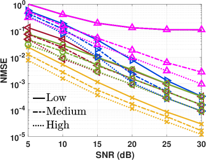
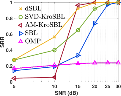
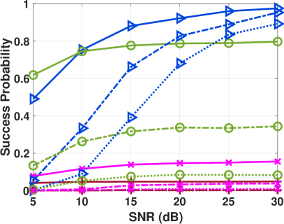
In this section, we highlight the advantages of the decomposition step in reducing computational complexity and enhancing the denoising effect. We focus on recovering the Kronecker-structured sparse vector (4) using a multidimensional BEM (3) in the on-grid setting, without requiring the OffSBL algorithm. By combining the decomposition step with SBL, we demonstrate the benefits of this approach. We compare our method’s performance with other methods that do not use decomposition, such as classical SBL [11], classical OMP, AM-KroSBL, and SVD-KroSBL [7]. Specifically, AM- and SVD-KroSBL only consider the Kronecker-structured support of the sparse vector and do not exploit the Kronecker structure in the nonzero entries as in (4).
We set with , and for in (3) and (4). So, we have and with . The columns of for are the steering vectors evaluated by the grids defined in Sec. IV. There are four nonzeros in each , whose positions are uniformly chosen from the grids and amplitudes are uniformly drawn from . Here, measurement level is set to be , labeled as Low, Medium, and High measurement case, controlling the number of measurements and the undersampling ratio . We adopt the additive white Gaussian noise with zero mean whose variance is determined by of . Three metrics are considered for performance evaluation: normalized mean squared error (NMSE), support recovery rate (SRR), and run time. Here, we define
where is the ground truth and is the estimated vector. We limit the number of iterations for the SBL-based methods (dSBL, cSBL, AM-KroSBL, and SVD-KroSBL) to 200 and prune small entries in hyperparameters for faster convergence.
The denoising effect of the decomposition step is shown in Table I. Here, we compare the noise levels of the original noisy signal in (3), the signal after decomposition where ’s are the solution to the problem (9), and the result of (19). It can be seen that the noise level is significantly reduced after decomposition. It also closely matches the result in (19), validating our claim on the denoising effect discussed in Sec. III-A.
Fig. 1 shows that with higher SNR and more measurements, all algorithms yield better NMSE and SRR, as expected. Our dSBL algorithm outperforms other methods in NMSE and has the best SRR performance in most cases, demonstrating the efficacy of the decomposition idea. In contrast to the SVD-KroSBL algorithm that uses Kronecker-structured support, dSBL achieves superior NMSE by using the additional Kronecker structure in nonzero entries explicitly enforced via (4) through the decomposition step. The relatively lower performance of AM-KroSBL is attributed to its slow convergence, given that we fix the number of EM iterations, as pointed out in [6]. The lower SRR and NMSE observed in the low SNR regime are due to small nonzero values in the estimate at locations where the ground truth is zero.
Finally, Table II demonstrates that dSBL requires two-order less run time than the other competing algorithms, corroborating the computational advantage of our decomposition.
| 5 dB | 10 dB | 15 dB | 20 dB | 25 dB | 30 dB | |
| 34.6609 | 9.5529 | 2.8528 | 0.9720 | 0.3044 | 0.0895 | |
| 0.9798 | 0.2720 | 0.0796 | 0.0267 | 0.0087 | 0.0023 | |
| From (19) | 0.9286 | 0.2580 | 0.0774 | 0.0263 | 0.0082 | 0.0024 |
| SNR | 5 dB | 10 dB | 15 dB | 20 dB | 25 dB | 30 dB |
| OMP | 0.599 | 0.602 | 0.605 | 0.603 | 0.604 | 0.603 |
| cSBL | 8.961 | 7.470 | 6.111 | 5.552 | 5.397 | 5.318 |
| AM-KroSBL | 8.528 | 8.516 | 7.249 | 5.424 | 4.520 | 4.093 |
| SVD-KroSBL | 4.534 | 3.360 | 2.840 | 2.668 | 2.627 | 2.608 |
| dSBL | 0.009 | 0.005 | 0.004 | 0.004 | 0.004 | 0.004 |
V-B Off-grid Parameters Estimation
| 20 | 25 | 30 | 35 | 40 | 45 | 50 | |
| OffSBL | 0.602 | 0.546 | 0.539 | 0.541 | 0.477 | 0.504 | 0.522 |
| SBL | 0.131 | 0.137 | 0.161 | 0.170 | 0.171 | 0.181 | 0.191 |
| LWSSBL | 0.032 | 0.033 | 0.035 | 0.037 | 0.038 | 0.041 | 0.043 |
| OGSBI | 0.250 | 0.269 | 0.274 | 0.286 | 0.290 | 0.305 | 0.315 |
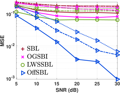
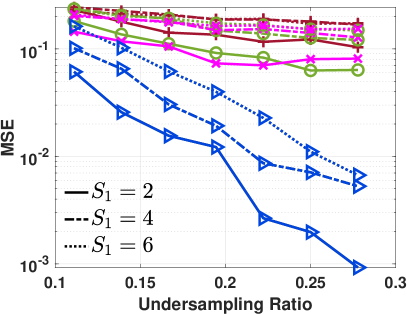
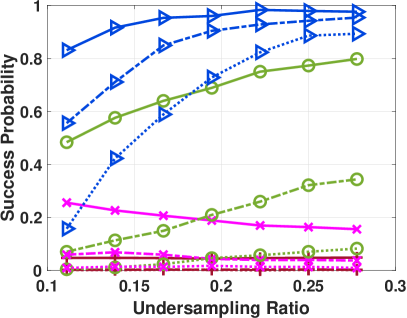
In this section, we apply OffSBL to the unknown parameters estimation problem. The model we consider here is the case in (28) with , where the goal is to estimate angles and coefficients . The column function is with , , and being the number of measurements. Here, is and controls the undersampling ratio defined as with . The matrix is randomly generated, whose entries take the form where is drawn from a uniform distribution on . We set the number of unknown parameters (angles) to be , and the angles are drawn sequentially from a uniform distribution on ensuring a minimal separation of . The coefficients are drawn from .
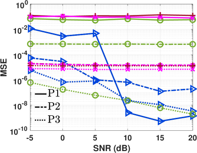
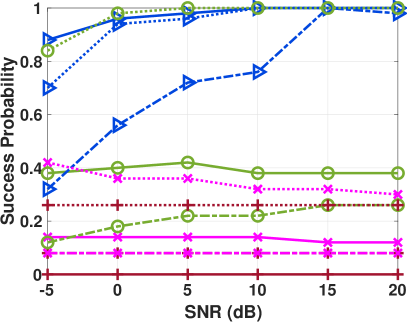
We use three benchmarks: (i) classical (on-grid) SBL, (ii) off-grid sparse Bayesian inference (OGSBI) using the first-order Taylor expansion [14], and (iii) light-weight sequential SBL (LWSSBL), a state-of-the-art off-grid method using marginal likelihood optimization [21]. In our simulations, we do not provide the number of unknowns to all algorithms, but only an upper bound of the number of unknowns. In practice, we only solve the problem (17) for the grid points corresponding to largest peaks of the hyperparameter instead of all grid points. Our OffSBL algorithm estimates the noise variance using (15). SBL and OGSBI can also estimate the noise variance, while noise variance estimation for LWSSBL is not discussed [21]. So for LWSSBL, we set noise variance estimate as as in [21]. We choose as in dB. To evaluate the performance of all schemes, we compare the mean squared error (MSE) and the success probability, where
with expectation taken over independent trials. Here, and denote the true value and the estimation, respectively. The success probability is defined as the fraction of trials with MSE smaller than .
We compare MSE and recovery probability for different SNRs and undersampling ratios in Fig. 2. We see that higher SNR and more measurements facilitate all algorithms, except OGSBI in Figs. 2(b) and 2(d). This is because OGSBI cannot effectively optimize the grid points in this setting, as we show later in Fig. 3. Among all candidates, our OffSBL has the best performance in both MSE and recovery probability in most cases. An exception is where LWSSBL has a higher success probability. However, LWSSBL often produces larger errors when it fails, making OffSBL superior in MSE.
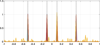
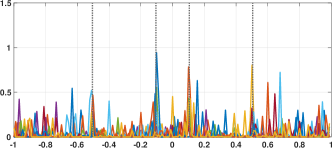
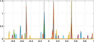
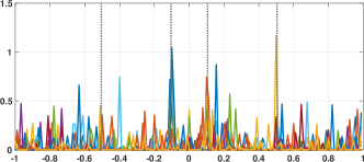
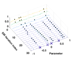
In Fig. 3, we present a worst-case scenario study. We set measurements and . The unknowns are , shown as vertical dashed lines in Figs. 3(a)-3(c). These values are intentionally selected to be midway between two grids to create a challenging case for grid optimization. All the coefficients are set to one. We provide the number of unknowns to all the algorithms but not the noise variance. We perform EM iterations to facilitate the convergence of all algorithms. The input of all algorithms is the same noiseless signal but with ten independent Gaussian noise realizations. We plot the final pseudospectrum (hyperparameter ) after EM iterations for ten noise realizations in Figs. 3(a)-3(c) with different colors.
Comparing the different algorithms, we note that OffSBL consistently recovers all parameters, with minimal amplitude spikes appearing in the pseudospectrum corresponding to parameters other than the true values. LWSSBL also recovers the unknowns but with a lower success probability. LWSSBL exhibits more peaks at parameters other than the true values, implying that it is more prone to being misled by incorrect columns in the dictionary due to its greedy nature. In contrast, while OffSBL takes longer to reach the final result (see Table III), evaluating all columns rather than proceeding greedily reduces the risk of being misled by incorrect columns.
Further, there is little difference between OGSBI and the on-grid benchmark SBL, indicating that the first-order approximation is less effective in this case. However, OGSBI has some improvement over SBL as reflected by a lower MSE. These findings also highlight that algorithms relying on on-grid SBL for rough estimates and then refining peaks are likely to fail, as on-grid SBL often doesn’t provide a reliable starting point, with peaks rarely matching the true parameters. This is likely due to the dictionary’s structure, which takes the form for some integer . When has fewer rows than columns , the compression effect from multiplication by can lead to information loss, creating a challenging setting for off-grid sparse recovery [37]. However, in many applications, such as IRS channel estimation, where the value of represents the number of time slots, is typically limited. Thus, integrating grid updates into the EM iteration, as implemented in OffSBL, is essential.
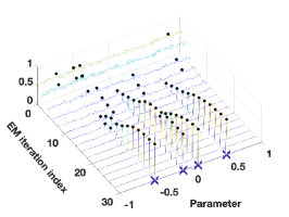
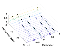
We further present the pseudospectrum for OffSBL, SBL, and OGSBI, along with the grid points that are updated dynamically throughout the EM iteration in Figs. 3(e)-3(f). Although SBL is an on-grid method, we still pinpoint the grids of the top four peaks. All algorithms have the same initially which becomes different afterward. Our OffSBL demonstrates superior optimization of grid points, identifying the correct values and amplitudes, whereas SBL and OGSBI do not reveal the true parameters. The evolution of the pseudospectrum across EM iterations highlights the effectiveness of our grid adjustment step.
V-C IRS-aided Wireless Channel Estimation
We focus on the IRS-aided channel estimation problem, as described in Sec. IV. Here, we first use the decomposition step and then turn to the BEM and apply OffSBL separately for in (28). Thus, the channel estimation scheme can be viewed as a collective evaluation of the decomposition and OffSBL. For benchmarking, we apply the same decomposition step, and then solve (28) using the same algorithms as in Sec. V-B. For simplicity, we denote the problem (28) with as P1, P2, and P3, respectively.
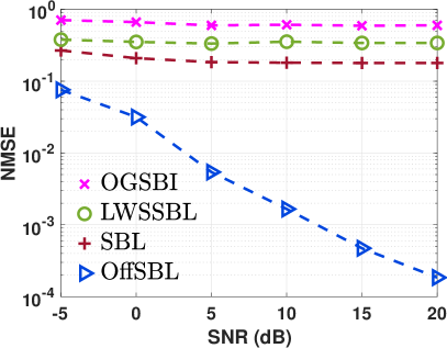
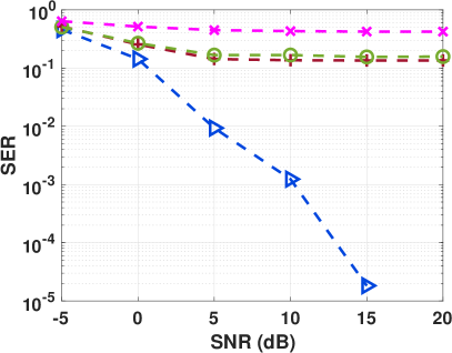
For IRS-aided channel estimation, we use BS antennas, MS antennas, IRS elements. We consider only one path between the BS and IRS[38, 39, 40, 41], as the IRS is typically mounted in locations with fewer obstacles[42, 43], and the line-of-sight path is generally much stronger than the other paths. Therefore, we take and . The IRS configuration entries are where is drawn uniformly randomly from . with . We send pilot signals for each IRS configuration. For our OffSBL algorithm, the dictionaries in P1, P2, and P3 are constructed by , , and , respectively. For the other algorithms, dictionaries are constructed using , , and grid points. The channel gains and in (23) and (24) are drawn from the standard complex Gaussian distribution [44]. We randomly draw , , , and from uniform distribution in , , , and , respectively. We also assume that the angles, after being spread, are separated by at least . We opt for SNR in dB. Along with MSE and success probability of the angle (parameter) estimation, we also use NMSE and symbol error rate (SER) to evaluate the channel estimation performance, where NMSE is
with being the channel estimate. We compute SER using -QAM symbols decoded using the estimated channel.
We first examine the angle estimation results in Fig. 4. It can be seen that our OffSBL can achieve the best performance in solving P1 and P2 except for the low SNR case for P2. P3 reduces to the normal DoA estimation problem, where LWSSBL exhibits superior recovery ability. However, at higher SNRs, our algorithm is able to achieve comparable performance. As evident from the NMSE and SER plots, OffSBL consistently recovers the true angles and accurately retrieves the coefficients, leading to the best NMSE and SER. Although other algorithms can perform well in solving P2 and P3, the significant recovery errors in P1 affect the overall accuracy of channel retrieval.
VI Conclusion
We addressed the joint estimation of unknown parameters and coefficients from Kronecker-structured measurements, focusing on IRS-aided wireless channel estimation. Leveraging the Kronecker structure, we decomposed the problem into smaller independent subproblems. Each subproblem was solved with EM-based SBL integrated with a novel grid optimization method to reduce grid mismatch. We provided a theoretical analysis of the error bound for the decomposition step and established the algorithm’s convergence. Our decomposition step also reduces the noise level in the measurements, which was also analyzed theoretically. Numerical results showed that the decomposition step reduces complexity, while the grid optimization improves accuracy. Future work can consider analyzing the resolution of the OffSBL method and extending our framework to the recovery of sparse tensors with ranks greater than one.
Appendix A Proof of Theorem 1
We define as the projection matrix onto the column space of a given matrix and as the projection onto its orthogonal subspace. Also, is the matrix spectral norm. We need the below lemma for the proof.
Lemma 3.
[45, Supplement Sec. 1.2] Suppose is a rank- matrix and where the entries of follow a zero mean Gaussian distribution with unit variance. We denote as the matrix of the right singular vectors of and the matrix of the top right singular vectors of , respectively. Suppose the th right singular value of satisfies for some large constant . Then, for all , there exist constants such that
and with probability exceeding ,
Here, where are the singular values of .
We prove Theorem 1 for using Lemma 3, and follow similarly. Also, we consider the decomposition of instead of . This scaling does not alter the subspaces obtained after decomposition but ensures that the noise entries follow a zero-mean, unit-variance Gaussian distribution, consistent with Lemma 3.
For , the true and estimated subspaces are spanned by and , respectively. The first mode matricization of the tensor , as defined in (6), is . Setting , and , and consequently, in Lemma 3, we derive
| (29) |
with probability at least .
Further, we bound using Lemma 3 by setting where ,
| (30) |
Then, we simplify the right-hand side of (30) using
| (31) |
Then, (30) is simplified as
for some constant . So, (29) and the union bound implies
| (32) |
with probability exceeding .
Furthermore, since , with , we derive
Consequently, because is greater than both roots of the quadratic function in . Thus, we deduce . So, from (32), we arrive at the desired result,
Appendix B Proof of Theorem 2
Our proof uses the following lemmas.
Lemma 4.
[27, Lemma 6]: Suppose are two matrices, and the projection matrix orthogonal to the subspace spanned by the leading left singular vectors of is . Then, , where is the rank of .
Lemma 5.
[46, Corollary 5.35] Let whose entries are independent Gaussian random variables with zero mean unit variance. Then, for any , the matrix satisfies , with probability less than .
Lemma 6.
[47, Lemma 8.1] Suppose satisfies the non-central distribution with degrees of freedom and non-centrality parameter . Then, for all , it satisfies with probability less than .
Lemma 7.
[26] Consider tensors , and , such that , where , for any compatible matrices . Then, .
Setting the tensor order and -ranks as for in [48, Eq. (19)] leads to (19). To prove the probabilistic bound, we note that using tensor notation, , where is HOSVD output and , with and being the measurement, the noiseless signal, and noise tensors, respectively, from (5).
HOSVD reconstructs . Here, , the leading left singular vectors of the th mode matricization of given by , with and are the th mode matricization of and , respectively. Also, , as the signal is real. Lemma 7 implies
where we define and with . Therefore,
| (33) |
To bound the first term in (33), let be the projection matrix orthogonal to so that , leading to
Therefore, using triangle inequality, we obtain
| (34) |
The last step follows from Lemma 4, as is the projection matrix orthogonal to and the rank of is 1 from (6). Also, Lemma 5 with and implies that with probability at least
From (34), with probability exceeding ,
| (35) |
Next, we bound the second term in (33). We note that is an -dimensional projection of a zero mean unit variance Gaussian tensor and follows [49, Supplement Sec. C.4]. Lemma 6 states that for any with probability exceeding . Setting and combining with (33) and (35) using the union bound yields (18) with probability exceeding . Hence, the proof is complete.
References
- [1] C. F. Caiafa and A. Cichocki, “Block sparse representations of tensors using Kronecker bases,” in Proc. IEEE Int. Conf. Acoust., Speech, Signal, Process., Mar. 2012, pp. 2709–2712.
- [2] C. F. Caiafa and A. Cichocki, “Computing sparse representations of multidimensional signals using Kronecker bases,” Neural Comput., vol. 25, no. 1, pp. 186–220, Jan. 2013.
- [3] C. F. Caiafa and A. Cichocki, “Multidimensional compressed sensing and their applications,” Wiley Interdiscip. Rev.: Data Min. Knowl. Discov., vol. 3, no. 6, pp. 355–380, Oct. 2013.
- [4] Z. Zhou, J. Fang, L. Yang, H. Li, Z. Chen, and R. S. Blum, “Low-rank tensor decomposition-aided channel estimation for millimeter wave MIMO-OFDM systems,” IEEE J. Sel. Areas Commun., vol. 35, no. 7, pp. 1524–1538, 2017.
- [5] R. Wang, H. Ren, C. Pan, G. Zhou, and J. Wang, “Tensor decomposition-based time varying channel estimation for mmWave MIMO-OFDM systems,” arXiv preprint arXiv:2403.02942, 2024.
- [6] Y. He and G. Joseph, “Bayesian algorithms for Kronecker-structured sparse vector recovery with application to IRS-MIMO channel estimation,” IEEE Trans. Signal Process., 2024.
- [7] Y. He and G. Joseph, “Structure-aware sparse Bayesian learning-based channel estimation for intelligent reflecting surface-aided MIMO,” in Proc. IEEE Int. Conf. Acoust., Speech, Signal, Process., Jun. 2023, pp. 1–5.
- [8] G. Ortiz-Jiménez, M. Coutino, S. P. Chepuri, and G. Leus, “Sparse sampling for inverse problems with tensors,” IEEE Trans. Signal Process., vol. 67, no. 12, pp. 3272–3286, 2019.
- [9] W.-C. Chang and Y. T. Su, “Sparse Bayesian learning based tensor dictionary learning and signal recovery with application to MIMO channel estimation,” IEEE J. Sel. Top. Signal Process., vol. 15, no. 3, pp. 847–859, Apr. 2021.
- [10] X. Xu, S. Zhang, F. Gao, and J. Wang, “Sparse Bayesian learning based channel extrapolation for RIS assisted MIMO-OFDM,” IEEE Trans. Commun., vol. 70, no. 8, pp. 5498–5513, Aug. 2022.
- [11] D. P. Wipf and B. D. Rao, “Sparse Bayesian learning for basis selection,” IEEE Trans. Signal Process., vol. 52, no. 8, pp. 2153–2164, Aug. 2004.
- [12] H. Zhu, G. Leus, and G. B. Giannakis, “Sparsity-cognizant total least-squares for perturbed compressive sampling,” IEEE Trans. Signal Process., vol. 59, no. 5, pp. 2002–2016, 2011.
- [13] G. Tang, B. N. Bhaskar, P. Shah, and B. Recht, “Compressed sensing off the grid,” IEEE Trans. Inf. Theory, vol. 59, no. 11, pp. 7465–7490, 2013.
- [14] Z. Yang, L. Xie, and C. Zhang, “Off-grid direction of arrival estimation using sparse Bayesian inference,” IEEE Trans. Signal Process., vol. 61, no. 1, pp. 38–43, 2012.
- [15] K. You, W. Guo, T. Peng, Y. Liu, P. Zuo, and W. Wang, “Parametric sparse Bayesian dictionary learning for multiple sources localization with propagation parameters uncertainty,” IEEE Trans. Signal Process., vol. 68, pp. 4194–4209, 2020.
- [16] M. Ibrahim, F. Römer, R. Alieiev, G. Del Galdo, and R. S. Thomä, “On the estimation of grid offsets in cs-based direction-of-arrival estimation,” in Proc. IEEE Int. Conf. Acoust., Speech, Signal, Process., 2014, pp. 6776–6780.
- [17] Y. Mao, Q. Guo, J. Ding, F. Liu, and Y. Yu, “Marginal likelihood maximization based fast array manifold matrix learning for direction of arrival estimation,” IEEE Trans. Signal Process., vol. 69, pp. 5512–5522, 2021.
- [18] J. Dai, A. Liu, and V. K. Lau, “FDD massive MIMO channel estimation with arbitrary 2D-array geometry,” IEEE Trans. Signal Process., vol. 66, no. 10, pp. 2584–2599, 2018.
- [19] A. Faul and M. Tipping, “Analysis of sparse Bayesian learning,” Adv. Neural Inf. Process. Syst., vol. 14, 2001.
- [20] Z.-M. Liu, Z.-T. Huang, and Y.-Y. Zhou, “An efficient maximum likelihood method for direction-of-arrival estimation via sparse Bayesian learning,” IEEE Trans. Wirel., vol. 11, no. 10, pp. 1–11, 2012.
- [21] R. R. Pote and B. D. Rao, “Light-weight sequential SBL algorithm: An alternative to OMP,” in Proc. IEEE Int. Conf. Acoust., Speech and Signal Process., 2023, pp. 1–5.
- [22] S. E. Ament and C. P. Gomes, “Sparse Bayesian learning via stepwise regression,” in Proc. Int. Conf. Mach. Learn. PMLR, 2021, pp. 264–274.
- [23] A. Lin, A. H. Song, B. Bilgic, and D. Ba, “Covariance-free sparse Bayesian learning,” IEEE Trans. Signal Process., vol. 70, pp. 3818–3831, Jun. 2022.
- [24] Y. He and G. Joseph, “Kronecker-structured sparse vector recovery with application to irs-mimo channel estimation,” arXiv preprint arXiv:2310.07869, 2023.
- [25] A. Cichocki, D. Mandic, L. De Lathauwer, G. Zhou, Q. Zhao, C. Caiafa, and H. A. Phan, “Tensor decompositions for signal processing applications: From two-way to multiway component analysis,” IEEE Signal Process. Mag., vol. 32, no. 2, pp. 145–163, 2015.
- [26] L. De Lathauwer, B. De Moor, and J. Vandewalle, “A multilinear singular value decomposition,” SIAM J. Matrix Anal. Appl., vol. 21, no. 4, pp. 1253–1278, 2000.
- [27] A. Zhang and D. Xia, “Tensor SVD: Statistical and computational limits,” IEEE Trans. Inf. Theory, vol. 64, no. 11, pp. 7311–7338, 2018.
- [28] G. Joseph and C. R. Murthy, “On the convergence of a Bayesian algorithm for joint dictionary learning and sparse recovery,” IEEE Trans. Signal Process., vol. 68, pp. 343–358, 2019.
- [29] S. Khanna and C. R. Murthy, “On the support recovery of jointly sparse gaussian sources via sparse bayesian learning,” IEEE Trans. Inf. Theory, vol. 68, no. 11, pp. 7361–7378, 2022.
- [30] C. J. Wu, “On the convergence properties of the EM algorithm,” Ann. Statist., pp. 95–103, Mar. 1983.
- [31] D. C. Araújo, A. L. De Almeida, J. P. Da Costa, and R. T. de Sousa, “Tensor-based channel estimation for massive MIMO-OFDM systems,” IEEE Access, vol. 7, pp. 42 133–42 147, Mar. 2019.
- [32] C. F. Van Loan, “The ubiquitous Kronecker product,” J. Comput. Appl. Math., vol. 123, no. 1-2, pp. 85–100, 2000.
- [33] C. R. Rao, “Estimation of heteroscedastic variances in linear models,” J. Am. Stat. Assoc., vol. 65, no. 329, pp. 161–172, Apr. 1970.
- [34] R. Schroeder, J. He, H. Djelouat, and M. Juntti, “Low-complexity near-field channel estimation for hybrid RIS assisted systems,” arXiv preprint arXiv:2404.17411, 2024.
- [35] J. Wang, J. Fang, and H. Li, “Intelligent reflecting surface-assisted NLOS sensing via tensor decomposition,” in Proc. EUSIPCO, Aug. 2024, pp. 1–5.
- [36] Y. Wang, G. Leus, and A. Pandharipande, “Direction estimation using compressive sampling array processing,” in IEEE Workshop Stat. Signal Process., 2009, pp. 626–629.
- [37] M. Guo, Y. D. Zhang, and T. Chen, “DOA estimation using compressed sparse array,” IEEE Trans. Signal Process., vol. 66, no. 15, pp. 4133–4146, 2018.
- [38] D. Dampahalage, K. S. Manosha, N. Rajatheva, and M. Latva-Aho, “Supervised learning based sparse channel estimation for RIS aided communications,” in Proc. IEEE Int. Conf. Acoust., Speech and Signal Process., 2022, pp. 8827–8831.
- [39] J. He, M. Leinonen, H. Wymeersch, and M. Juntti, “Channel estimation for RIS-aided mmWave MIMO systems,” in Proc. IEEE Glob. Commun. Conf., Feb. 2020, pp. 1–6.
- [40] Z. Wan, Z. Gao, F. Gao, M. Di Renzo, and M.-S. Alouini, “Terahertz massive MIMO with holographic reconfigurable intelligent surfaces,” IEEE Trans. Commun., vol. 69, no. 7, pp. 4732–4750, Mar. 2021.
- [41] L. Yashvanth and C. R. Murthy, “Cascaded channel estimation for distributed IRS aided mmwave massive MIMO systems,” in Proc. IEEE Glob. Commun. Conf., Dec. 2022, pp. 717–723.
- [42] B. Zheng, C. You, W. Mei, and R. Zhang, “A survey on channel estimation and practical passive beamforming design for intelligent reflecting surface aided wireless communications,” IEEE Commun. Surv. Tutor., vol. 24, no. 2, pp. 1035–1071, Feb. 2022.
- [43] Y. Liu, X. Liu, X. Mu, T. Hou, J. Xu, M. Di Renzo, and N. Al-Dhahir, “Reconfigurable intelligent surfaces: Principles and opportunities,” IEEE Commun. Surv. Tutor., vol. 23, no. 3, pp. 1546–1577, 2021.
- [44] Y. Lin, S. Jin, M. Matthaiou, and X. You, “Channel estimation and user localization for IRS-assisted MIMO-OFDM systems,” IEEE Trans. Wireless Commun., vol. 21, no. 4, pp. 2320–2335, Apr. 2021.
- [45] T. T. Cai and A. Zhang, “Rate-optimal perturbation bounds for singular subspaces with applications to high-dimensional statistics,” Ann. Stat., vol. 46, no. 1, pp. 60 – 89, 2018.
- [46] R. Vershynin, “Introduction to the non-asymptotic analysis of random matrices,” arXiv preprint arXiv:1011.3027, 2010.
- [47] L. Birgé, “An alternative point of view on Lepski’s method,” Lecture Notes-Monograph Series, pp. 113–133, 2001.
- [48] E. R. Balda, S. A. Cheema, J. Steinwandt, M. Haardt, A. Weiss, and A. Yeredor, “First-order perturbation analysis of low-rank tensor approximations based on the truncated HOSVD,” in Proc. Asilomar Conf. Signals Syst. Comput., 2016, pp. 1723–1727.
- [49] A. Zhang and R. Han, “Optimal sparse singular value decomposition for high-dimensional high-order data,” J. Am. Stat. Assoc., 2019.