Enumeration algorithms for combinatorial problems using Ising machines

Abstract

Combinatorial problems such as combinatorial optimization and constraint satisfaction problems arise in decision-making across various fields of science and technology. In real-world applications, when multiple optimal or constraint-satisfying solutions exist, enumerating all these solutions—rather than finding just one—is often desirable, as it provides flexibility in decision-making. However, combinatorial problems and their enumeration versions pose significant computational challenges due to combinatorial explosion. To address these challenges, we propose enumeration algorithms for combinatorial optimization and constraint satisfaction problems using Ising machines. Ising machines are specialized devices designed to efficiently solve combinatorial problems. Typically, they sample low-cost solutions in a stochastic manner. Our enumeration algorithms repeatedly sample solutions to collect all desirable solutions. The crux of the proposed algorithms is their stopping criteria for sampling, which are derived based on probability theory. In particular, the proposed algorithms have theoretical guarantees that the failure probability of enumeration is bounded above by a user-specified value, provided that lower-cost solutions are sampled more frequently and equal-cost solutions are sampled with equal probability. Many physics-based Ising machines are expected to (approximately) satisfy these conditions. As a demonstration, we applied our algorithm using simulated annealing to maximum clique enumeration on random graphs. We found that our algorithm enumerates all maximum cliques in large dense graphs faster than a conventional branch-and-bound algorithm specially designed for maximum clique enumeration. This demonstrates the promising potential of our proposed approach.

I Introduction

Combinatorial optimization and constraint satisfaction play significant roles in decision-making across scientific research, industrial development, and other real-life problem-solving. Combinatorial optimization is the process of selecting an optimal option, in terms of a specific criterion, from a finite discrete set of feasible alternatives. In contrast, constraint satisfaction is the process of finding a feasible solution that satisfies specified constraints without necessarily optimizing any criterion. Combinatorial problems—which encompass combinatorial optimization problems and constraint satisfaction problems—arise in various real-world applications, including chemistry and materials science [1, 2, 3], drug discovery [4], system design [5], operational scheduling and navigation [6, 7, 8], finance [9], and leisure [10].

Enumerating all optimal or constraint-satisfying solutions is often desirable in practical applications [1, 2, 11, 12]. The target solutions of combinatorial problems (i.e., optimal or constraint-satisfying solutions) are not necessarily unique. When multiple target solutions exist, enumerating all these solutions—rather than finding just one—provides flexibility in decision-making. This allows decision-makers to choose solutions that best fit additional preferences or constraints not captured in the initial problem modeling.

Despite their practical importance, combinatorial problems and their enumeration versions pose significant computational challenges. Many combinatorial problems are known to be NP-hard [13]; in the worst-case scenarios, the computation time to solve such a problem increases exponentially with the problem size. Moreover, enumerating all solutions generally requires more computational effort than finding just one solution. To address these challenges, we propose enumeration algorithms for combinatorial problems using Ising machines.

Ising machines are specialized devices designed to efficiently solve combinatorial problems [14]. The term “Ising machine” comes from their specialization in finding the ground states of Ising models (or spin glass models) in the statistical physics of magnets. Several seminal studies on computations utilizing Ising models were published in the 1980s , including the Hopfield network [16, 17] with its application to combinatorial optimization [6], the Boltzmann machine [18], and simulated annealing (SA) [5]. During the same period, early specialized devices for Ising model simulation were also developed [19, 20]. More recently, quantum annealing (QA) was proposed in 1998 [21] and physically implemented in 2011 [22]. Furthermore, the quantum approximate optimization algorithm (QAOA) [23], running on gate-type quantum computers, typically targets Ising model problems. Currently, various types of Ising machines are available, as reviewed in [14].

Many combinatorial problems are efficiently reducible to finding the ground states of Ising models [24, 25]. Ising model problems are NP-hard [26]; thus, any NP problems can be mapped to Ising model problems in theory. Furthermore, the real-world applications mentioned above can also be mapped to Ising model problems [1, 2, 3, 4, 5, 6, 7, 8, 9, 10]. Therefore, Ising machines are widely applicable to real-world combinatorial problems.

A key feature of Ising machines, especially those based on statistical, quantum, or optical physics, is that most of them can be regarded as samplers from low energy states of Ising models. For instance, SA simulates the thermal annealing process of Ising models, where the system temperature gradually decreases. If the cooling schedule is sufficiently slow, the system is expected to remain in thermal equilibrium during the annealing process, so the final state distribution is close to the Boltzmann (or Gibbs) distribution at a low temperature. In fact, the sampling probability distribution converges to the uniform measure on the ground states, i.e., the Boltzmann distribution at absolute zero temperature, for a sufficiently slow annealing schedule [27]. Furthermore, quantum and optical Ising machines, such as (noisy) QA devices [28, 29, 30], QAOA [31, 32], coherent Ising machines (CIMs) [4], and quantum bifurcation machines (QbMs) [33], have theoretical or empirical evidence that they approximately realize Boltzmann sampling at a low effective temperature.

We utilize Ising machines as samplers to enumerate all ground states of Ising models. By repeatedly sampling states using Ising machines, one can eventually collect all ground states in the limit of infinite samples . This raises a fundamental practical question: When should we stop sampling? In this article, we address this question and derive effective stopping criteria based on probability theory.

The remainder of this article is organized as follows. In Sec. II, we formulate the combinatorial problems and Ising model problems considered in this article, and define energy-ordered fair Ising machines and cost-ordered fair samplers as sampler models. These sampler models are necessary for deriving appropriate stopping criteria for sampling. In Sec. III, we propose enumeration algorithms for constraint satisfaction problems (Algorithm 1) and combinatorial optimization problems (Algorithm 2). These algorithms have theoretical guarantees that the failure probability of enumeration is bounded above by a user-specified value $\epsilon$ when using a cost-ordered fair sampler (or an energy-ordered fair Ising machine). Detailed theoretical analysis of the failure probability is provided in Appendix A. Furthermore, in Sec. IV, we present a numerical demonstration where we applied Algorithm 2 using SA to maximum clique enumeration on random graphs. Finally, we conclude in Sec. V.

II Problem Formulation and Sampler Models

II.1 Combinatorial Problems and Ising Models

The combinatorial problems we consider in this article are generally formulated as

$$\operatorname*{minimize}_{x\in X}\ f(x),$$ (1)

where $X$ is the finite discrete set of feasible solutions, and $f\colon X\to\mathbb{R}$ is the cost function to be minimized. If $f$ is a constant function, there is no preference between alternatives, so all feasible solutions are target solutions; that is, the problem is a constraint satisfaction problem. Otherwise, it is a (single-objective) combinatorial optimization problem. Typically, $x$ is represented as an integer vector, and the feasible set $X$ is defined by equality or inequality constraints on $x$.

In many cases, the combinatorial problem defined in Eq. (1) can be mapped to an Ising model problem:

$$\operatorname*{minimize}_{\bm{\sigma}\in\{-1,1\}^{N}}\ H_{\mathrm{Ising}}(\bm{\sigma}).$$ (2)

The Ising Hamiltonian $H_{\mathrm{Ising}}$ is defined as

$$H_{\mathrm{Ising}}(\bm{\sigma})=-\sum_{i=1}^{N-1}\sum_{j=i+1}^{N}J_{ij}\sigma_{i}\sigma_{j}-\sum_{i=1}^{N}h_{i}\sigma_{i}.$$ (3)

Here, $N$, $\sigma_{i}$, $J_{ij}$, and $h_{i}$ denote, respectively, the number of spin variables, the $i$th spin variable, the interaction coefficient between two spins $\sigma_{i}$ and $\sigma_{j}$, and the local field interacting with $\sigma_{i}$. This Ising model should be designed such that the ground states correspond to the target solutions of the original problem. Standard techniques for mapping combinatorial problems into Ising model problems can be found in [24, 25].

II.2 Cost-Ordered Fair Samplers

To derive appropriate stopping criteria for sampling, we need to specify a class of samplers (or sampling probability distributions) to be considered. In this subsection, we define two classes of samplers, energy-ordered fair Ising machines for Ising model problems and cost-ordered fair samplers for general combinatorial problems. In brief, these sampler models capture the following desirable features of samplers for optimization: more preferred solutions are sampled more frequently, and equally preferred solutions are sampled with equal probability.

First, let us introduce two conditions regarding the sampling probability distribution of an Ising machine, denoted by $p_{\mathrm{Ising}}$. For any two spin configurations $\bm{\sigma}_{1}$ and $\bm{\sigma}_{2}$,

$$\begin{cases}H_{\mathrm{Ising}}(\bm{\sigma}_{1})<H_{\mathrm{Ising}}(\bm{\sigma}_{2})\Rightarrow p_{\mathrm{Ising}}(\bm{\sigma}_{1})\geq p_{\mathrm{Ising}}(\bm{\sigma}_{2}),\\ H_{\mathrm{Ising}}(\bm{\sigma}_{1})=H_{\mathrm{Ising}}(\bm{\sigma}_{2})\Rightarrow p_{\mathrm{Ising}}(\bm{\sigma}_{1})=p_{\mathrm{Ising}}(\bm{\sigma}_{2}).\end{cases}$$ (4)

The first condition—referred to as the energy-ordered sampling condition—asserts that a spin configuration with lower energy is sampled more frequently (or at least with the same frequency) than a spin configuration with higher energy. In contrast, the second condition—referred to as the fair sampling condition—states that two spin configurations with equal energy are sampled with equal probability. For example, the Boltzmann distribution satisfies these two conditions. Therefore, it is expected that the following Ising machines can be utilized as (approximate) energy-ordered fair Ising machines for appropriate parameter regimes (e.g., a sufficiently slow annealing schedule), as they are (approximate) Boltzmann samplers: SA devices [27], (noisy) QA devices [28, 29, 30], gate-type quantum computers with QAOA [31, 32], CIMs [4], and QbMs [33]. Since the energy-ordered and fair sampling conditions are weaker than the Boltzmann sampling condition, a broader class of Ising machines could be utilized as energy-ordered fair Ising machines.

Next, we extend the concept of energy-ordered fair Ising machines to cost-ordered fair samplers for general combinatorial problems. We define the cost-ordered and fair sampling conditions regarding a sampling probability distribution over feasible solutions of the combinatorial problem defined in Eq. (1), denoted by $p$, as follows. For any two feasible solutions $x_{1}$ and $x_{2}$,

$$\begin{cases}f(x_{1})<f(x_{2})\Rightarrow p(x_{1})\geq p(x_{2}),\\ f(x_{1})=f(x_{2})\Rightarrow p(x_{1})=p(x_{2}).\end{cases}$$ (5)

We define cost-ordered fair samplers as samplers that generate only feasible solutions and follows a probability distribution satisfying the conditions in Eq. (5). Since Ising model problems are a subset of combinatorial problems, and all spin configurations are feasible solutions in Ising model problems, energy-ordered fair Ising machines are also cost-ordered fair samplers for the Ising model problems.

Cost-ordered fair samplers for general combinatorial problems can be implemented by using energy-ordered fair Ising machines. Typical Ising formulations of combinatorial problems preserve the order of preference among solutions [24, 25]:

$$\begin{cases}f(x_{1})<f(x_{2})\Rightarrow H_{\mathrm{Ising}}(\bm{\sigma}_{1})<H_{\mathrm{Ising}}(\bm{\sigma}_{2}),\\ f(x_{1})=f(x_{2})\Rightarrow H_{\mathrm{Ising}}(\bm{\sigma}_{1})=H_{\mathrm{Ising}}(\bm{\sigma}_{2}),\end{cases}$$ (6)

where $\bm{\sigma}_{1}$ and $\bm{\sigma}_{2}$ are the spin configurations corresponding to feasible solutions $x_{1}$ and $x_{2}$, respectively. Under this condition, the probability distribution over feasible solutions generated by an energy-ordered fair Ising machine satisfies the cost-ordered and fair sampling conditions as defined in Eq. (5). Note that not all possible spin configurations that can be sampled by the Ising machine correspond to feasible solutions of the original problem. However, such infeasible solutions can be rejected during sampling by checking constraint satisfaction, so that the sampler generates only feasible solutions following the cost-ordered fair sampling probability distribution. (This rejection process will also be illustrated in the next section.)

In the next section, we will present enumeration algorithms for combinatorial problems using cost-ordered fair samplers. Although we primarily focus on cost-ordered fair samplers implemented using energy-ordered fair Ising machines, our enumeration algorithms can employ a wider class of stochastic methods and computing devices that satisfy the conditions in Eq. (5). Additionally, the proposed algorithms can still work effectively even if the sampler employed does not strictly meet the conditions in Eq. (5) (see also Sec. IV). However, the success probability has no theoretical guarantee in such cases.

III Algorithms

This section describes our proposed algorithms that enumerate all solutions to (1) a constraint satisfaction problem and (2) a combinatorial optimization problem using an Ising machine.

III.1 Preliminaries: Coupon Collector’s Problem

Our enumeration algorithms involve stopping criteria inspired by the coupon collector’s problem, a classic problem in probability theory. This problem considers the scenario where one needs to collect all distinct items (coupons) through uniformly random sampling. For example, the number of samples necessary to collect all distinct items in a set of cardinality $n$, denoted by $T^{(n)}_{n}$, has the following tail distribution:

$$P\left(T^{(n)}_{n}>\left\lceil n\ln\frac{n}{\epsilon}\right\rceil\right)<\epsilon,$$ (7)

where $\lceil\ \rceil$ denotes the ceiling function, and $\epsilon$ is any positive number less than one. (See also Lemma 1 in Apppendix A.2.) This inequality suggests that when sampling is stopped at $\lceil n\ln(n/\epsilon)\rceil$, the failure probability of collecting all items is less than $\epsilon$. Therefore, we could employ $\lceil n\ln(n/\epsilon)\rceil$ as the deadline for collecting all target solutions, if the number of target solutions $n$ were known in advance. However, the value of $n$ is unknown in practice. Furthermore, in a combinatorial optimization problem, nonoptimal solutions are also sampled in addition to optimal solutions. These challenges demand an extension of the theory of the coupon collector’s problem, which we address in this article.

In the following two subsections, we expound our enumeration algorithms based on the extended theory of the coupon collector’s problem. Mathematical details are presented in Appendix A.

III.2 Enumeration Algorithm for Constraint Satisfaction Problems

First, we present an enumeration algorithm for constraint satisfaction problems, referred to as Algorithm 1 in this article. Algorithm 1 requires that the constraint satisfaction problem to be solved have at least one feasible solution and that a fair sampler of feasible solutions be available. Note that for a constraint satisfaction problem, the cost function $f$ is considered constant; thus the cost-ordered sampling condition is not required. The pseudocode is shown in Fig. 1.

Figure 1: Pseudocode of Algorithm 1. The function SAMPLE is a fair sampler of feasible solutions. The definition of $\kappa_{1}(\epsilon)$, which appears in line 6, is provided in Eq. (8). The failure probability of Algorithm 1 is theoretically guaranteed to be less than the user-specified failure tolerance $\epsilon$ (see Theorem 1 in Appendix A.2).

Algorithm 1 repeatedly samples feasible solutions for a constraint satisfaction problem using the function SAMPLE. This function returns a feasible solution uniformly at random. Such a fair sampler can be implemented using a fair Ising machine that samples each ground state of an Ising model with equal probability. In general, it is easy to check whether a solution satisfies the constraints; thus, SAMPLE can return only feasible solutions by discarding infeasible samples generated by the Ising machine.

As the sampling process is repeated and the number of samples $\tau$ approaches infinity, the set of collected solutions $S$ converges to the set of all feasible solutions. To stop the sampling process after a finite number of samples, Algorithm 1 sets the deadline for collecting $m$ distinct solutions as $\lceil m\ln(m\kappa_{1}/\epsilon)\rceil$ for $m=2,3,\dots$. Here, $\epsilon$ is a tolerable failure probability for the enumeration and is required to be less than $1/\mathrm{e}\ (\simeq 0.37)$. Note that we typically set the tolerable failure probability $\epsilon$ to a much smaller value, such as 0.01 (1%), so this requirement on $\epsilon$ is not severe. The factor $\kappa_{1}$ depends on $\epsilon$ but not on the unknown number of target solutions to be enumerated. It is defined as

$$\kappa_{1}\coloneqq\frac{3^{-2\alpha}}{1-\mathrm{e}^{-\beta}}+\frac{1}{1-\mathrm{e}^{-\frac{\alpha}{\mathrm{e}-1}}},$$ (8)

where

$$\alpha \coloneqq\ln\frac{1}{\epsilon}-1,$$ (9)

$$\beta \coloneqq\frac{\frac{1}{\mathrm{e}}+\frac{1}{3}\ln\frac{1}{3}}{\frac{1}{\mathrm{e}}-\frac{1}{3}}\alpha.$$ (10)

For instance, $\kappa_{1}\simeq 1.14$ when $\epsilon=0.01$. Intuitively, the constant $\kappa_{1}$—which is always larger than one—can be regarded as a “correction” factor to the original deadline in the coupon collector’s problem. It slightly extends the deadline to compensate for the increased error chances caused by the lack of information about the number of target solutions (see Appendix A.2 for detailed discussion). If the number of collected solutions is fewer than $m$ at $\tau=\lceil m\ln(m\kappa_{1}/\epsilon)\rceil$, Algorithm 1 stops the sampling. These specific deadlines ensure that the failure probability for the enumeration remains below $\epsilon$, as stated by Theorem 1 in Appendix A.2.

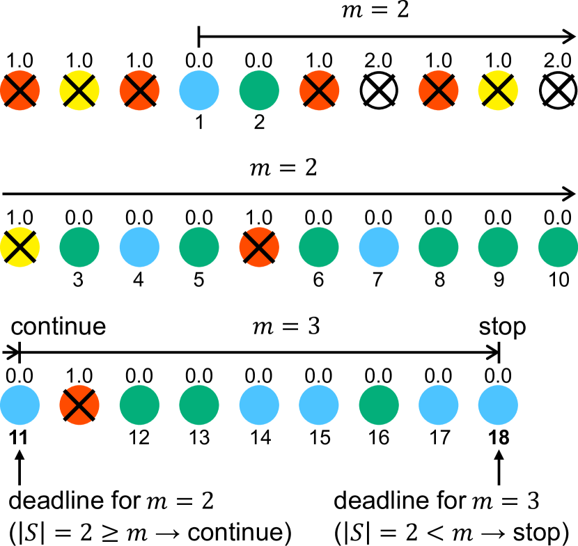
Figure 2: An illustration of the sampling process in Algorithm 1. Each circle represents a sample generated by an Ising machine, with different colors indicating different solutions. The value above each circle indicates the energy of the corresponding solution. In this example, the ground state energy is 0.0, so light-blue and green circles represent feasible solutions. In contrast, circles of other colors correspond to infeasible solutions, which are discarded during the sampling process, as indicated by “x” marks. The numbers below the feasible solutions indicate the sample count $\tau$. The deadlines for $m=2$ and $3$ were calculated as $\lceil m\ln(m\kappa_{1}/\epsilon)\rceil$ with $\epsilon=0.01$.

Figure 2 illustrates the sampling process in Algorithm 1. Each circle represents a sample generated by an Ising machine. During the sampling process, samples with energy higher than the ground state energy of 0.0 (i.e., infeasible solutions) are discarded, as indicated by “x” marks. This discarding process is part of the SAMPLE subroutine in the pseudocode; thus, SAMPLE returns only feasible solutions without “x” marks. After sampling the first feasible solution (the first light-blue one), Algorithm 1 continues sampling until the deadline for collecting $m=2$ distinct solutions. This deadline is $\lceil 2\ln(2\kappa_{1}/\epsilon)\rceil$, which equals 11 for $\epsilon=0.01$. Note that the sample count $\tau$, indicated by numbers under the circles of feasible solutions, is incremented only when a feasible solution is sampled. At the deadline $\tau=11$, the set of collected solutions $S$ contains two distinct feasible solutions (the light-blue and green ones). Since the number of collected solutions $|S|$ equals $m=2$, Algorithm 1 proceeds to the next phase, aiming to collect $m=3$ distinct solutions. The next deadline is $\lceil 3\ln(3\kappa_{1}/\epsilon)\rceil$, which equals 18. However, at the deadline $\tau=18$, the number of collected solutions $|S|$ is still two, which is fewer than the goal value $m=3$. Therefore, Algorithm 1 stops sampling and returns the set $S$ containing the two distinct feasible solutions.

III.3 Enumeration Algorithm for Combinatorial Optimization Problems

Next, we present an enumeration algorithm for combinatorial optimization problems, referred to as Algorithm 2 in this article. Algorithm 2 requires that the combinatorial optimization problem to be solved have at least one feasible solution and that a cost-ordered fair sampler of feasible solutions be available. The pseudocode is shown in Fig. 3.

Figure 3: Pseudocode of Algorithm 2. The function SAMPLE is a cost-ordered fair sampler of feasible solutions. The definition of $\kappa_{2}(\epsilon)$, which appears in line 5, is provided in Eq. (11). The failure probability of Algorithm 2 is theoretically guaranteed to be less than the user-specified failure tolerance $\epsilon$ (see Theorem 2 in Appendix A.3).

Enumerating all optimal solutions poses a challenge that does not arise in enumerating all feasible solutions: it is impossible to judge whether a sampled solution is optimal or not without knowing the minimum cost value in advance. Therefore, Algorithm 2 collects current best solutions as provisional target solutions during sampling. If a solution better than the provisional target solutions is sampled, the algorithm discards the already collected solutions and continues to collect new provisional target solutions. As this process is repeated, the set of collected solutions is expected to converge to the set of all optimal solutions.

Specifically, Algorithm 2 holds the minimum cost value among already sampled solutions in variable $\theta$. To collect provisional target solutions with cost value $\theta$, the algorithm uses the subroutine ENUMERATE. This subroutine is a modified version of Algorithm 1, which aims to enumerate all feasible solutions with cost value $\theta$. However, if a solution with cost value lower than $\theta$ is sampled during enumeration, this subroutine stops collecting solutions with cost value $\theta$ and resets the set of collected target solutions $S$. In either case, the subroutine returns $S$ and the current minimum cost value. If the ENUMERATE subroutine stops enumeration without sampling a better solution (i.e., the current minimum cost value does not change), Algorithm 2 halts and returns $S$.

The deadline for collecting $m$ distinct solutions employed in the ENUMERATE subroutine depends on $\kappa_{2}$, instead of $\kappa_{1}$ which is used in Algorithm 1. The constant $\kappa_{2}$ is defined as

$$\kappa_{2}\coloneqq\frac{4^{\alpha}}{1-\mathrm{e}^{-\beta}}\left(\zeta(2\alpha)-\sum_{k=1}^{5}\frac{1}{k^{2\alpha}}\right)+\frac{2-\mathrm{e}^{-\frac{\alpha}{\mathrm{e}-1}}}{\left(1-\mathrm{e}^{-\frac{\alpha}{\mathrm{e}-1}}\right)^{2}},$$ (11)

where $\alpha$ and $\beta$ are the same as those used in Eq. (8), and $\zeta$ denotes the Riemann zeta function. If $\epsilon$ is less than $1/\mathrm{e}^{1.5}(\simeq 0.22)$, the Riemann zeta function $\zeta(2\alpha)$ converges, because the argument $2\alpha=2[\ln(1/\epsilon)-1]$ is greater than one. Note that this upper limit for allowable $\epsilon$ value is moderate, as we typically set the tolerable failure probability to a much smaller value, such as 0.01 (1%). For instance, when $\epsilon=0.01$, $\kappa_{2}\simeq 2.44$. This specific design of $\kappa_{2}$ ensures that the failure probability for the enumeration remains below $\epsilon$, as stated by Theorem 2 in Appendix A.3.

The deadlines used in Algorithm 2 are longer than those in Algorithm 1 (see also Figs. 2 and 4). This is because $\kappa_{2}$ is always larger than $\kappa_{1}$, in order to compensate for the increased error chances caused by the lack of the information about the true minimum cost (see the end of Appendix A.3 for detailed discussion).

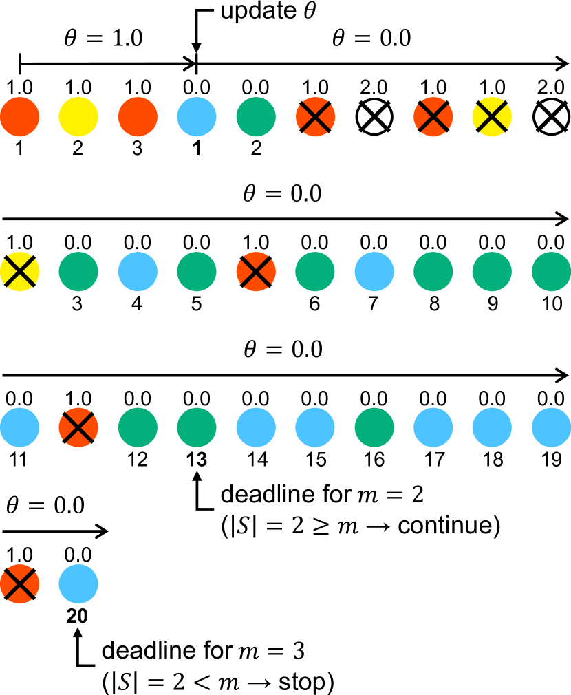
Figure 4: An illustration of the sampling process in Algorithm 2. Each circle represents a sample generated by an Ising machine, with different colors indicating different solutions. The “x” marks indicate the rejection of the samples. The value above each circle indicates the energy of the corresponding solution. Here, for simplicity, the energy of each feasible solution is set to its cost value in the original problem. In this example, the ground state energy is 0.0, so light-blue and green circles represent the optimal solutions. The numbers below the accepted solutions indicate the sample count $\tau$. Note that the sample count is reset when the current minimum cost value $\theta$ is updated. The deadlines for $m=2$ and $3$ were calculated as $\lceil m\ln(m\kappa_{2}/\epsilon)\rceil$ with $\epsilon=0.01$. The sample sequence is the same as that in Fig. 2.

Figure 4 illustrates the sampling process in Algorithm 2. In contrast to Algorithm 1, Algorithm 2 does not reject the first sample (the first red one) that is not a true target solution. Instead, the algorithm collects it as a provisional target solution and sets $\theta$ to its cost value 1.0. At this first stage, the algorithm aims to collect all provisional target solutions with cost value 1.0 (the red and yellow ones). However, before the deadline for collecting $m=2$ distinct solutions with cost value 1.0, a better solution (the first light-blue one) is sampled. Thus, the algorithm updates $\theta$ to 0.0 and resets $S$ and the sample count $\tau$. At this second stage, the algorithm aims to collect all provisional target solutions with cost value 0.0 (the light-blue and green ones). Solutions with cost value exceeding the new threshold $\theta=0.0$ are rejected during sampling, as indicated by the “x” marks. Because $\theta=0.0$ is the true minimum of the cost function in this example, no better solutions than the provisional target solutions are sampled during the enumeration with $\theta=0.0$. Consequently, the algorithm continues the enumeration until the deadline for $m=3$ without updating $\theta$. Since the number of optimal solutions is two, the algorithm halts at this deadline, returning $S$ that contains the two optimal solutions.

III.4 Computational Complexity

Before concluding this section, we discuss the computational complexity of the proposed enumeration algorithms. Both Algorithm 1 and Algorithm 2 require $\lceil(n+1)\ln[(n+1)\kappa/\epsilon]\rceil$ samples of target solutions to ensure successful collection of all $n$ target solutions, where $\kappa$ is either $\kappa_{1}$ or $\kappa_{2}$. (Note that the algorithms stop at the deadline for collecting $n+1$ distinct target solutions in successful cases.) On the other hand, the expected time to sample a target solution can be estimated by $\mathcal{T}_{\mathrm{sample}}/p_{\mathrm{target}}$. Here, $\mathcal{T}_{\mathrm{sample}}$ denotes the time to sample a feasible solution (including both target and nontarget ones) using a cost-ordered fair sampler, and $p_{\mathrm{target}}$ represents the probability that the sampler generates a target solution, i.e. $p_{\mathrm{target}}=\sum_{x\in\operatorname{argmin}_{x^{\prime}}f(x^{\prime})}p(x)$. Combining these estimates, we obtain the expected computation time of the proposed algorithms as:

$$\left\lceil(n+1)\ln\frac{(n+1)\kappa}{\epsilon}\right\rceil\times\frac{\mathcal{T}_{\mathrm{sample}}}{p_{\mathrm{target}}}.$$ (12)

Although the first factor does not directly depend on the problem size (e.g., the number of variables), the second factor may increase exponentially with the problem size for NP-hard problems. Therefore, the computation time is mainly dominated by the second factor, i.e., the sampling performance of the cost-ordered fair sampler (or the Ising machine employed). Moreover, the number of target solutions $n$ may also increase exponentially with the problem size in worst-case scenarios.

An enumeration algorithm for constraint satisfaction problems utilizing a fair Ising machine was previously proposed by Kumar et al. [35] and later improved by Mizuno and Komatsuzaki [36]. Their algorithm is the direct ancestor of Algorithm 1 proposed in this article. In their algorithm, the deadlines for collecting $m$ distinct solutions are set at large intervals (e.g., $m=2,2^{2},\cdots,2^{N}$, where $N$ is the number of spin variables). This leads to additional overhead in the number of samples required. For instance, when $n=20$, the required number of samples is $\lceil 32\ln(32\kappa/\epsilon)\rceil$ in their algorithm. In contrast, our Algorithm 1 requires a much smaller number of samples, $\lceil 21\ln(21\kappa_{1}/\epsilon)\rceil$, because in Algorithm 1, the deadlines are set at every integer value of $m$. Furthermore, the factor $\kappa$ in the previous algorithm is typically proportional to $N$, while $\kappa_{1}$ used in our Algorithm 1 is independent of $N$. This improvement in the computational complexity of Algorithm 1 results from the careful analysis of the failure probability, which is detailed in Appendix A.2.

IV Numerical Demonstration

This section presents a numerical demonstration of Algorithm 2, the enumeration algorithm for combinatorial optimization problems proposed in Sec. III.3. As discussed in Sec. III.4, the actual computation time of the algorithm depends on the performance of the Ising machine employed. Furthermore, although the algorithm has the theoretical guarantee on its success rate under the cost-ordered fair sampling model, the success rate could be different from the theoretical expectation due to deviations in the actual sampling probability from the theoretical model. Therefore, we evaluated the actual computation time and success rate of Algorithm 2 for the maximum clique problem, a textbook example of combinatorial optimization.

IV.1 Maximum Clique Problem

A clique in an undirected graph $G$ is a subgraph in which every two distinct vertices are adjacent in $G$. Finding a maximum clique, i.e., a clique with the largest number of vertices, is a well-known NP-hard combinatorial optimization problem [13, 24, 37]. The maximum clique problem has a wide range of real-world applications from chemoinformatics to social network analysis [37]. In particular, enumerating all maximum cliques is desirable in applications to chemoinformatics [2] and bioinformatics [11].

The maximum clique problem on graph $G$ can be formulated as:

$$\operatorname*{maximize}_{\bm{x}\in\{0,1\}^{|V_{G}|}} \sum_{v\in V_{G}}x_{v},$$ (13)

$$\operatorname{subject\ to} \forall\{u,v\}\in\overline{E}_{G},\;x_{u}x_{v}=0,$$

where $V_{G}$ and $\overline{E}_{G}$ denote the vertex set and the complementary edge set (i.e., the set of nonadjacent vertex pairs) of $G$, respectively. The symbol $\bm{x}$ collectively denotes the binary variables $\{x_{v}\}_{v\in V_{G}}$ and represents a subset of vertices in $G$. Here, each variable $x_{v}$ indicates whether the vertex $v$ is included in the subset ($x_{v}=1$) or not ($x_{v}=0$). The constraints ensure that the vertex subset does not include any nonadjacent vertex pairs. In other words, these constraints exclude vertex subsets that do not form a clique. Under the clique constraints, the objective is to maximize the number of vertices included, which equals $\sum_{v\in V_{G}}x_{v}$.

Alternatively, the maximum clique problem can be formulated as a quadratic unconstrained binary optimization (QUBO) problem:

$$\operatorname*{minimize}_{\bm{x}\in\{0,1\}^{|V_{G}|}}\quad-\sum_{v\in V_{G}}x_{v}+A\sum_{\{u,v\}\in\overline{E}_{G}}x_{u}x_{v},$$ (14)

where $A$ is a positive constant that controls the penalty for violating the clique constraints. If $A$ is greater than one, the optimal solutions of this QUBO formulation are exactly the same as those of the original formulation [24]. By converting the binary variables $x_{v}$ to spin variables $\sigma_{v}\ (\coloneqq 1-2x_{v})$, the QUBO problem becomes equivalent to finding the ground state(s) of an Ising model.

IV.2 Computation Methods

We generated Erdős-Rényi random graphs [38] to create benchmark problems. The number of vertices of each graph $G$, denoted by $|V_{G}|$, was randomly selected from the range of 10 to 500. The number of edges was determined to achieve an approximate graph density $D$, calculated as $\binom{|V_{G}|}{2}D$ rounded to the nearest integer. The graph density parameter $D$ was set to 0.25, 0.5, and 0.75. For each value of $D$, 100 random graphs were generated.

We solved the maximum clique problem on each graph using Algorithm 2 with simulated annealing (SA). The algorithm was implemented in Python, employing the SimulatedAnnealingSampler from the D-Wave Ocean Software [39]. The tolerant failure probability $\epsilon$ was set to 0.01. The penalty strength $A$ in Eq. (14) was set to a moderate value of two, as an excessively large penalty strength may deteriorate the performance of SA. Additionally, we used default parameters for the SA function.

We also solved the same problems using a conventional branch-and-bound algorithm as a reference. This branch-and-bound algorithm is based on the Bron–Kerbosch algorithm [40] with a pivoting technique proposed by Tomita, Tanaka, and Takahashi [41]. This standard algorithm is implemented in the NetworkX package [42], called find_cliques. We further modified this find_cliques function by incorporating a basic bounding condition for efficient maximum clique search proposed by Carraghan and Pardalos [43]. This algorithm is exact, i.e., it enumerates all maximum cliques with a 100% success probability.

All computations were performed on a Linux machine equipped with two Intel Xeon Platinum 8360Y processors (2.40 GHz, 36 cores each).

IV.3 Results and Discussion

IV.3.1 Computation time

First, we compare the computation times of our proposed algorithm (Algorithm 2 using SA) and the conventional algorithm (Bron–Kerbosch combined with the enhancements by Tomita–Tanaka–Takahashi and Carraghan–Pardalos). The results are shown in Fig. 5 and Table 1. For dense and large random graphs with a graph density of 0.75 and more than 355 vertices, the conventional algorithm did not finish even after 10 days had passed. Therefore, we omit these computationally demanding instances from the comparison.

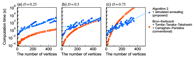
Figure 5: Computation times required to enumerate all maximum cliques in random graphs with different graph densities $D$ and different numbers of vertices. The blue circles indicate the computation times of Algorithm 2 using SA. For each data point, the mean computation time of all successful cases out of 100 independent runs was calculated. The relative standard errors have a mean of 0.01 and a maximum of 0.07; thus, the error bars (not shown) are shorter than the diameter of the blue circles. The sky-blue dashed lines represent linear fits to the computation times indicated by the blue circles for graphs with more than 250 vertices. The red diamonds indicate the computation times of the conventional algorithm (Bron–Kerbosch combined with the enhancements by Tomita–Tanaka–Takahashi and Carraghan–Pardalos). For cases with computation times shorter than seven days, the average of 10 independent runs was taken. For cases with computation times longer than seven days, only one run was conducted to evaluate the computation time. The relative standard errors have a mean of 0.02 and a maximum of 0.33; thus, the error bars (not shown) are shorter than the size of the red diamonds. The light-pink dashed lines represent linear fits to the computation times indicated by the red diamonds for graphs with more than 250 vertices.

Table 1: Computation time scaling with respect to the number of vertices $|V_{G}|$, computed through the linear fitting shown in Fig. 5.

Density $D$	Algorithm 2 + SA	Conventional Algorithm
0.25	$O(1.015^{\|V_{G}\|})$	$O(1.010^{\|V_{G}\|})$
0.5	$O(1.010^{\|V_{G}\|})$	$O(1.017^{\|V_{G}\|})$
0.75	$O(1.025^{\|V_{G}\|})$	$O(1.038^{\|V_{G}\|})$

In terms of the computation time scaling with respect to the number of vertices, the performance of the conventional algorithm is more susceptible to the graph density than that of Algorithm 2 using SA. The rate of increase in the computation time of the conventional algorithm become significantly higher as the graph density increases. In contrast, the rate of increase in the computation time of Algorithm 2 only modestly changes with the graph density. Consequently, for sparse graphs with $D=0.25$, the conventional algorithm exhibits better performance than Algorithm 2, while for denser graphs with $D=0.5$ and $0.75$, our Algorithm 2 outperforms the conventional algorithm.

Furthermore, we have found that our Algorithm 2 using SA requires less computation times than the conventional algorithm also for maximum clique problems that arise in a chemoinformatics application—atom-to-atom mapping. This result has been reported in a separate paper [2]. This improvement in the required computation time contributes to achieving accurate and practical atom-to-atom mapping without relying on chemical rules and machine learning.

These results do not demonstrate that our algorithm is better than any existing algorithm for maximum clique enumeration on any graph. However, the fact that our algorithm—which uses the general-purpose SA—exhibits superior performance to one of the conventional algorithms specially designed for maximum clique enumeration is noteworthy. This superiority in dense random graphs and real chemical applications suggests the promising potential of our proposed algorithm.

IV.3.2 Success rate

Next, we examine the success rate of Algorithm 2. The statistics of the number of successes are shown in Fig. 6.

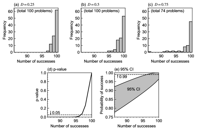
Figure 6: Statistics of the number of successes of Algorithm 2. Panels (a)–(c) display histograms of the number of successes out of 100 independent runs for problems with different graph densities. Panel (d) shows the p-values for each observed number of successes, representing the probability of obtaining that number or fewer successes under the hypothesis that the true success probability is 0.99. Panel (e) presents the 95% confidence intervals (CIs) [44, 45] (also referred to as compatibility intervals [46]) for the estimated success probability based on each observed number of successes.

A number of successes fewer than 97 is considered incompatible with the theoretical guarantee that the success probability of Algorithm 2 is greater than 0.99 when $\epsilon=0.01$. This assessment is based on the criteria that the p-value is less than 0.05 and/or the 95% CI does not include 0.99 [see Fig. 6(d) and (e)]. There is no such incompatibility for the 100 problems with $D=0.25$. However, four problems with $D=0.5$ and ten problems with $D=0.75$ exhibit such incompatibility. Additionally, in all failure runs, the algorithm successfully identifies at least one maximum clique but fails to find some of the maximum cliques. These observation suggest that the ground-state sampling using SA does not always satisfy the fair sampling condition.

To assess the fairness of the ground-state sampling using SA, we conducted chi-squared tests for each problem, using samples obtained during the 100 independent runs of Algorithm 2. The results are shown in Fig. 7 and Table 2.

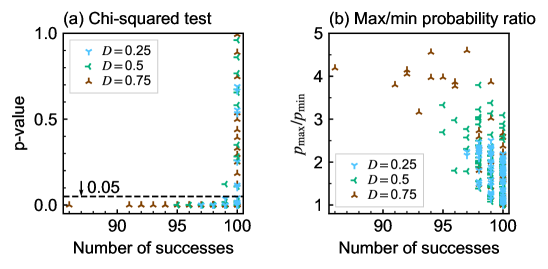
Figure 7: Fairness of the ground-state sampling using SA. Panel (a) shows the relationship between the number of successes and the p-value of the chi-squared test, assessing the fairness of the ground-state sampling. A p-value closer to 0 suggests that the observed sampling frequencies are unlikely under the hypothesis that the ground-state sampling is fair. For problems with a unique ground state, the p-values are undefined; thus, data points for these problems are not plotted in this panel. Panel (b) presents the correlation between the number of successes and the ratio of the maximum and minimum sampling probabilities among ground states, denoted by $p_{\mathrm{max}}/p_{\mathrm{min}}$. This ratio is also an indicator of the fairness of the ground-state sampling: the closer it is to 1, the more fair the ground-state sampling is.

Table 2: Number of problems in each category, defined as follows: All refers to all problems solved. Unique denotes problems with a unique ground state. “Fair” (respectively, “Unfair”) represents problems with multiple ground states where the ground-state sampling using SA has a p-value of the chi-squared test greater than or equal to (respectively, less than) 0.05. Note that categorizing sampling probability distributions as “fair” and “unfair” based on the p-values is not definitive; it only indicates whether each distribution is considered compatible with the fair sampling condition or not under the specified criterion. Additionally, numbers in parentheses indicate the number of problems where the number of successes was less than 97, suggesting incompatibility with the theoretical guarantee of Algorithm 2 under the criteria shown in Fig. 6.

Density $D$	All	Unique	“Fair”	“Unfair”
0.25	100 (0)	16 (0)	8 (0)	76 (0)
0.5	100 (4)	17 (0)	11 (0)	72 (4)
0.75	74 (10)	11 (0)	12 (0)	51 (10)

In Table 2, we tentatively categorize sampling probability distributions on multiple ground states into “fair” and “unfair” based on the p-values of the chi-squared tests. Numbers in parentheses in the table indicate the number of problems where the number of successes is fewer than 97, suggesting incompatibility with the theoretical guarantee of Algorithm 2. From the table, it is clear that all cases incompatible with the theoretical guarantee are assigned to “unfair”, as we expected. Furthermore, it is worth noting that there are many “unfair” cases with estimated success probability compatible with 0.99. These facts can also be confirmed from Fig. 7(a).

As another indicator of the fairness of the ground-state sampling, we also calculated the ratio of the maximum and minimum sampling probabilities among ground states, denoted by $p_{\mathrm{max}}/p_{\mathrm{min}}$. Figure 7(b) indicates a moderate negative correlation between the number of successes and $p_{\mathrm{max}}/p_{\mathrm{min}}$, with Pearson correlation coefficient -0.69. As expected, larger variation in the sampling probability tends to result in fewer successes.

Finally, we calculated the solution coverage defined as the number of collected solutions divided by the total number of the target solutions. For any problem solved, the mean solution coverage of the 100 runs is greater than or equal to 0.99. This implies that even though the algorithm fails to enumerate all target solutions, only a few solutions are uncollected. Indeed, the number of uncollected solutions in failure runs is typically one, and two or more uncollected solutions are observed only in seven problems.

In summary, the ground-state sampling using SA is not necessarily fair under the present setting. However, our Algorithm 2 still works effectively even for such “unfair” cases with high success probability and/or high solution coverage, though there is no theoretical guarantee on the success probability for such cases yet. To theoretically ensure the success probability, one can employ other samplers such as the Grover-mixer quantum alternating operator ansatz algorithm [47], for which the fair sampling condition is theoretically guaranteed. Alternatively, it should be helpful to extend the present algorithm and theory to allow variation in the sampling probability up to a user-specified value of $p_{\mathrm{max}}/p_{\mathrm{min}}$.

V Conclusions

We have developed enumeration algorithms for combinatorial problems, specifically (1) constraint satisfaction and (2) combinatorial optimization problems, using Ising machines as solution samplers. Appropriate stopping criteria for solution sampling have been derived based on the cost-ordered fair sampler model. If the solution sampling satisfies the cost-ordered and fair sampling conditions, the proposed algorithms have theoretical guarantees that the failure probability is below a user-specified value $\epsilon$. Various types of physics-based Ising machines can likely be employed to implement (approximate) cost-ordered fair samplers. Even though the sampling process does not strictly satisfy the cost-ordered and fair sampling conditions, the proposed algorithms may still function effectively with high success probability and/or high solution coverage, as demonstrated for the maximum clique enumeration using SA. Furthermore, we showed that our Algorithm 2 using SA outperforms a conventional algorithm for maximum clique enumeration on dense random graphs and a chemoinformatics application [2].

The proposed algorithms rely on the cost-ordered fair sampler model: more preferred solutions are sampled more frequently, and equally preferred solutions are sampled with equal probability. Although this model captures desirable features of samplers for optimization and serves as an archetypal model for this initial algorithm development, relaxing the cost-ordered and/or fair sampling conditions should be helpful for expanding the applicable domain of sampling-based enumeration algorithms.

Moreover, although we focus on using Ising machines in this article, the proposed algorithms can be combined with any types of solution samplers considered as (approximate) cost-ordered fair samplers. For example, when combined with a Boltzmann sampler of molecular structures (in an appropriate discretized representation), our algorithm can determine when to stop exploring the molecular energy landscape without missing the global minima. Developing sampling-based enumeration algorithms combined with samplers in various fields should also be a promising research direction.

We hope the enumeration algorithms proposed in this article will contribute to future technological advancements in sampling-based enumeration algorithms and their interdisciplinary applications.

Appendix A Theoretical Analysis

This appendix presents a theoretical analysis of the failure probabilities of Algorithms 1 and 2 proposed in this article.

A.1 Notation

Let $X$ be a finite set with cardinality $n$, and let $p\colon X\to[0,1]$ be a discrete probability distribution (probability mass function) on $X$. Consider the sampling process from $X$, comprising independent trials, each of which is governed by $p$. We define random variables involved in the sampling process under the probability distribution $p$ as follows :

• $x^{(p)}_{\tau}$: The item sampled on the $\tau$th trial. By definition, $P(x^{(p)}_{\tau}=x)=p(x)$ for any $x\in X$.

• $S^{(p)}_{\tau}$: The set of distinct items that have been sampled by the $\tau$th trial.

• $\mathfrak{x}^{(p)}_{i}$: The $i$th distinct item sampled during the process; that is, the $i$th new distinct item not previously sampled.

• $\mathfrak{S}^{(p)}_{i}$: The set of the first $i$ distinct sampled items, i.e., $\{\mathfrak{x}_{j}^{(p)}\mid j=1,\dots,i\}$.

• $T^{(p)}_{m}$: The number of trials needed to collect $m$ distinct items; equivalently, the trial number at which the $m$th distinct item $\mathfrak{x}^{(p)}_{i}$ is first sampled.

• $t^{(p)}_{m}$: The number of trials needed to sample the $m$th distinct item after having sampled $m-1$ distinct items, i.e., $T^{(p)}_{m}-T^{(p)}_{m-1}$.

For instance, in the sample sequence—red (trial 1), yellow (trial 2), red (trial 3), and blue (trial 4):

• $x^{(p)}_{3}=\text{red}$, $\mathfrak{x}^{(p)}_{3}=\text{blue}$.

• $S^{(p)}_{3}=\{\text{red},\text{yellow}\}$, $\mathfrak{S}^{(p)}_{3}=\{\text{red},\text{yellow},\text{blue}\}$.

• $T^{(p)}_{3}=4$, $t^{(p)}_{3}=2$.

Furthermore, we define $S^{(p)}_{0}$ and $\mathfrak{S}^{(p)}_{0}$ as the empty set and $T^{(p)}_{0}$ as zero, initializing the process. In the special case where $p$ is the discrete uniform distribution, we replace the superscript $(p)$ in the notation by $(n)$ (the cardinality of $X$), e.g., $T^{(n)}_{m}$.

A.2 Failure Probability of Algorithm 1

In this subsection, we evaluate the failure probability of Algorithm 1. Since Algorithm 1 utilizes a fair sampler of feasible solutions, we consider that $X$ is the feasible solution set with cardinality $n$ and the sampling probability distribution $p$ is the discrete uniform distribution on $X$. Furthermore, Algorithm 1 samples one feasible solution at the beginning (see line 1 in the pseudocode), so Algorithm 1 always succeeds when $n=1$. Hence, we consider $n\geq 2$.

Algorithm 1 succeeds in enumerating all $n$ feasible solutions only when it meets all deadlines for collecting $m$ distinct feasible solutions ($m=2,\dots,n$). In other words, if $T^{(n)}_{m}>\lceil m\ln(m\kappa_{1}/\epsilon)\rceil$ for some $m$, Algorithm 1 halts before collecting all feasible solutions. Therefore, the failure probability of Algorithm 1 is bounded above by the sum of $P(T^{(n)}_{m}>\lceil m\ln(m\kappa_{1}/\epsilon)\rceil)$ over $m=2,\dots,n$. Thus, our primary goal is to evaluate the tail distribution of $T^{(n)}_{m}$.

We start by evaluating the simplest case where $m=n$, which corresponds to the classical coupon collector’s problem.

Lemma 1.

Suppose $X$ is a finite set with cardinality $n$ and $p$ is the discrete uniform distribution on $X$. Let $\epsilon$ be a positive real number less than one. In the sampling process dictated by $p$, the probability that $T^{(n)}_{n}$ exceeds $\lceil n\ln(n/\epsilon)\rceil$ is less than $\epsilon$:

$$P\left(T^{(n)}_{n}>\left\lceil n\ln\frac{n}{\epsilon}\right\rceil\right)<\epsilon.$$ (15)

Proof.

The probability that an element $x\in X$ has not been sampled yet up to the $\tau$th trial is given by

$$P\left(x\notin S^{(n)}_{\tau}\right)=\left(1-\frac{1}{n}\right)^{\tau}<\mathrm{e}^{-\frac{\tau}{n}}.$$ (16)

Since $T^{(n)}_{n}>\tau$ means that there exists $x\in X$ that has not been sampled yet up to $\tau$, the tail distribution of $T^{(n)}_{n}$ can be evaluated as follows:

$$P\left(T^{(n)}_{n}>\tau\right) =P\left(\bigcup_{x\in X}\{x\notin S^{(n)}_{\tau}\}\right)$$

$$\leq\sum_{x\in X}P\left(x\notin S^{(n)}_{\tau}\right)$$

$$<n\mathrm{e}^{-\frac{\tau}{n}}.$$ (17)

By substituting $\lceil n\ln(n/\epsilon)\rceil$ for $\tau$ in the above equation, we establish the inequality to be proved. ∎

Next, we generalize Lemma 1 to arbitrary $m\ (\leq n)$.

Lemma 2.

Suppose $X$ is a finite set with cardinality $n$ and $p$ is the discrete uniform distribution on $X$. Let $\epsilon$ be a positive real number less than one. In the sampling process dictated by $p$, for a positive integer $m\ (\leq n)$, the probability that $T^{(m)}_{n}$ exceeds $\lceil m\ln(m/\epsilon)\rceil$ is bounded from above as follows:

$$P\left(T^{(n)}_{m}>\left\lceil m\ln\frac{m}{\epsilon}\right\rceil\right)<\left(\frac{m}{n}\right)^{\left\lceil{m\ln\frac{m}{\epsilon}}\right\rceil+1}\binom{n}{m}\epsilon.$$ (18)

Proof.

The random variable $t^{(n)}_{i}$ follows the geometric distribution given by

$$P\left(t^{(n)}_{i}=\tau_{i}\right)=\left(\frac{i-1}{n}\right)^{\tau_{i}-1}\frac{n-(i-1)}{n}.$$ (19)

This is because the event that $t^{(n)}_{i}$ equals $\tau_{i}$ occurs when the following two conditions are met. First, during the first $\tau_{i}-1$ trials, the sampler generates any of the $i-1$ already-sampled items. Second, on the $\tau_{i}$th trial, it samples one of the $n-(i-1)$ items not previously sampled. Furthermore, the random variables $t^{(n)}_{1},t^{(n)}_{2},\dots,t^{(n)}_{m}$ are mutually independent, as the sampling trials are independent. Consequently, we obtain

$$P\left(t^{(n)}_{1}=\tau_{1},t^{(n)}_{2}=\tau_{2},\dots,t^{(n)}_{m}=\tau_{m}\right)$$

$$=\prod_{i=1}^{m}\left(\frac{i-1}{n}\right)^{\tau_{i}-1}\frac{n-(i-1)}{n}$$

$$=\frac{1}{n^{\tau^{\prime}}}\frac{n!}{(n-m)!}\prod_{i=1}^{m}(i-1)^{\tau_{i}-1},$$ (20)

where $\tau^{\prime}=\sum_{i=1}^{m}\tau_{i}$, and the last step follows the equation $\prod_{i=1}^{m}[n-(i-1)]=n!/(n-m)!$.

The random variable $T^{(n)}_{m}$ can be expressed as $t^{(n)}_{1}+t^{(n)}_{2}+\cdots+t^{(n)}_{m}$. If $t^{(n)}_{i}=\tau_{i}$ for each $i$ from $1$ to $m$, any combination of positive integers $\tau_{1},\tau_{2},\dots,\tau_{m}$, satisfying the condition $\tau_{1}+\tau_{2}+\cdots+\tau_{m}=\tau^{\prime}$, results in $T^{(n)}_{m}=\tau^{\prime}$. Let us introduce the set of such combinations, which is given by

$$\mathcal{C}_{m}(\tau^{\prime})\coloneqq$$

$$\left\{(\tau_{1},\tau_{2},\dots,\tau_{m})\in\mathbb{N}^{m}\ \middle|\ \tau_{1}+\tau_{2}+\cdots+\tau_{m}=\tau^{\prime}\right\}.$$ (21)

Now the tail distribution of $T^{(n)}_{m}$ can be written as

$$P\left(T^{(n)}_{m}>\tau\right)$$

$$=\sum_{\tau^{\prime}=\tau+1}^{\infty}\sum_{\bm{\tau}_{1:m}\in\mathcal{C}_{m}(\tau^{\prime})}P\left(t^{(n)}_{1}=\tau_{1},t^{(n)}_{2}=\tau_{2},\dots,t^{(n)}_{m}=\tau_{m}\right)$$

$$=\sum_{\tau^{\prime}=\tau+1}^{\infty}\sum_{\bm{\tau}_{1:m}\in\mathcal{C}_{m}(\tau^{\prime})}\frac{1}{n^{\tau^{\prime}}}\frac{n!}{(n-m)!}\prod_{i=1}^{m}(i-1)^{\tau_{i}-1},$$ (22)

where $\tau$ is an arbitrary positive integer, and $\bm{\tau}_{1:m}$ denotes a tuple $(\tau_{1},\tau_{2},\dots,\tau_{m})$ collectively. The second summation over $\bm{\tau}_{1:m}$ on the right-hand side accounts for every possible combination of $\tau_{1},\tau_{2},\dots,\tau_{m}$ that satisfies $T^{(n)}_{m}=\tau^{\prime}$. The first summation over $\tau^{\prime}$ covers all cases where $T^{(n)}_{m}$ exceeds $\tau$.

We further transform the above equation as follows:

$$P\left(T^{(n)}_{m}>\tau\right)$$

$$=\sum_{\tau^{\prime}=\tau+1}^{\infty}\sum_{\bm{\tau}_{1:m}\in\mathcal{C}_{m}(\tau^{\prime})}\left(\frac{m}{n}\right)^{\tau^{\prime}}\frac{n!}{(n-m)!m!}\frac{m!}{m^{\tau^{\prime}}}\prod_{i=1}^{m}(i-1)^{\tau_{i}-1}$$

$$\leq\left(\frac{m}{n}\right)^{\tau+1}\binom{n}{m}\sum_{\tau^{\prime}=\tau+1}^{\infty}\sum_{\bm{\tau}_{1:m}\in\mathcal{C}_{m}(\tau^{\prime})}\frac{m!}{m^{\tau^{\prime}}}\prod_{i=1}^{m}(i-1)^{\tau_{i}-1}$$

$$=\left(\frac{m}{n}\right)^{\tau+1}\binom{n}{m}P\left(T^{(m)}_{m}>\tau\right).$$ (23)

In the transformation from the first line to the second line, we replace the factor $(m/n)^{\tau^{\prime}}$ with $(m/n)^{\tau+1}$ because $(m/n)\leq 1$ and $\tau^{\prime}\geq\tau+1$. The last step of the transformation is according to Eq. (22) where $n$ is replaced by $m$. Substituting $\lceil m\ln(m/\epsilon)\rceil$ for $\tau$ in the above equation and applying Lemma 1 complete the proof. ∎

This tail distribution estimate may be roughly interpreted as follows: Consider an event where the sampler generates solutions only from a subset of $X$ with cardinality $m$. The probability that this event occurs at least until the $(\tau+1)$th trial is $(m/n)^{\tau+1}$. Furthermore, under this event, the probability that the number of trials needed to collect all $m$ solutions in this subset exceeds $\tau$ is $P(T^{(m)}_{m}>\tau)$. Considering all possible combinations of $m$ solutions from $X$, an upper bound for the probability that $T^{(n)}_{m}$ exceeds $\tau$ would be given by

$$\binom{n}{m}\left(\frac{m}{n}\right)^{\tau+1}P\left(T^{(m)}_{m}>\tau\right).$$ (24)

This expression appears in the last equation of the above proof.

We now have an upper bound estimate for the tail distribution of $T^{(n)}_{m}$. To calculate an upper bound for the failure probability of Algorithm 1, we will sum $P(T^{(n)}_{m}>\lceil m\ln(m\kappa_{1}/\epsilon)\rceil)$ over $m=2$ to $n$. However, the upper bound for the tail distribution derived in Lemma 2 is still complex and difficult to sum over $m$. Therefore, our next goal is to simplify the right-hand side of the inequality in Lemma 2.

Lemma 3.

Let $n$ and $m$ be positive integers satisfying $2\leq m\leq n$, and let $\epsilon$ be a positive real number less than one. Then, the following inequality holds:

$$\left(\frac{m}{n}\right)^{\left\lceil{m\ln\frac{m}{\epsilon}}\right\rceil}\binom{n}{m}<\left(\frac{m}{n}\right)^{\alpha m},$$ (25)

where $\alpha\coloneqq\ln(1/\epsilon)-1$.

Proof.

Define a function $g$ by the following expression:

$$g(u)\coloneqq\left(\frac{m}{u}\right)^{\left\lceil{m\ln\frac{m}{\epsilon}}\right\rceil}\frac{\prod_{i=1}^{m}[u-(i-1)]}{m!}\quad(u\geq m).$$ (26)

The inequality to be proven can be expressed as $g(n)\leq(m/n)^{\alpha m}$. Differentiating $\ln g(u)$ with respect to $u$ gives

$$\frac{\mathrm{d}}{\mathrm{d}u}\ln g(u) =-\frac{\left\lceil{m\ln\frac{m}{\epsilon}}\right\rceil}{u}+\sum_{i=1}^{m}\frac{1}{u-(i-1)}$$

$$=\frac{1}{u}\left[\sum_{i=1}^{m}\frac{u}{u-(i-1)}-\left\lceil{m\ln\frac{m}{\epsilon}}\right\rceil\right].$$ (27)

The summation $\sum_{i=1}^{m}u/[u-(i-1)]$ decreases as $u$ increases. Hence, for $u\geq m$, the summation is upper bounded by $\sum_{i=1}^{m}m/[m-(i-1)]\ [=m(1+1/2+\dots+1/m)]$, which is the $m$th harmonic number multiplied by $m$. Furthermore, the $m$th harmonic number ($m\geq 2$) can be evaluated as

$$\sum_{i=1}^{m}\frac{1}{m-(i-1)} =1+\sum_{k=2}^{m}\frac{1}{k}$$

$$<1+\int_{1}^{m}\frac{\mathrm{d}s}{s}$$

$$=1+\ln m.$$ (28)

Therefore, we obtain

$$\frac{\mathrm{d}}{\mathrm{d}u}\ln g(u) <\frac{1}{u}\left[m(1+\ln m)-m\ln\frac{m}{\epsilon}\right]$$

$$=-\frac{\alpha m}{u},$$ (29)

where $\alpha=\ln(1/\epsilon)-1$. Integrating both sides of this inequality from $m$ to $n$ yields

$$\ln\frac{g(n)}{g(m)}<-\alpha m\ln\frac{n}{m}.$$ (30)

Because $g(m)=1$, this inequality implies

$$g(n)=\left(\frac{m}{n}\right)^{\left\lceil{m\ln\frac{m}{\epsilon}}\right\rceil}\binom{n}{m}<\left(\frac{m}{n}\right)^{\alpha m}.$$ (31)

This concludes the proof. ∎

We further simplify the upper bound as follows:

Lemma 4.

Let $n$ and $m$ be positive integers satisfying $m\leq n$, and let $\alpha$ be a positive real number. Then the following inequalities hold:

$$\left(\frac{m}{n}\right)^{\alpha m} \leq\left(\frac{2}{n}\right)^{2\alpha}\mathrm{e}^{-\beta(m-2)}, \text{if}\quad 2\leq m<\frac{n}{\mathrm{e}},$$ (32)

$$\left(\frac{m}{n}\right)^{\alpha m} \leq\mathrm{e}^{\frac{\alpha}{\mathrm{e}-1}(m-n)}, \text{if}\quad\frac{n}{\mathrm{e}}<m\leq n,$$ (33)

where $\beta$ is defined as

$$\beta\coloneqq\frac{\frac{1}{\mathrm{e}}+\frac{1}{3}\ln\frac{1}{3}}{\frac{1}{\mathrm{e}}-\frac{1}{3}}\alpha.$$ (34)

Proof.

The left-hand side of the inequalities can be written as

$$\left(\frac{m}{n}\right)^{\alpha m}=\exp\left(n\alpha\left(\frac{m}{n}\right)\ln\left(\frac{m}{n}\right)\right).$$ (35)

To evaluate the exponent in the above equation, we examine a function $h$ defined as

$$h(u)\coloneqq u\ln u$$ (36)

for $u\in[2/n,1]$. Here, the range of $u$ corresponds to $2\leq m\leq n$ via the relation $u=m/n$. The graph of $v=u\ln u$ is shown in Fig. 8.

Figure 8: The graph of $v=u\ln u$. The straight lines (1) and (2) provide upper bounds for the value of $u\ln u$ in the intervals $[2/n,1/\mathrm{e}]$ and $[1/\mathrm{e},1]$, respectively. These lines are used to prove the two inequalities in this lemma.

The function $h$ is convex. Therefore, for all $u_{1},u_{2}\in[2/n,1]$ and all $\lambda\in[0,1]$,

$$h((1-\lambda)u_{1}+\lambda u_{2})\leq(1-\lambda)h(u_{1})+\lambda h(u_{2}).$$ (37)

This inequality is equivalent to

$$h(u)\leq h(u_{1})+\frac{h(u_{2})-h(u_{1})}{u_{2}-u_{1}}(u-u_{1}),$$ (38)

where $u\ [=(1-\lambda)u_{1}+\lambda u_{2}]$ lies between $u_{1}$ and $u_{2}$. The right-hand side of Eq. (38) represents the line passing through points $(u_{1},h(u_{1}))$ and $(u_{2},h(u_{2}))$. We apply this inequality to two intervals: $[2/n,1/\mathrm{e}]$ and $[1/\mathrm{e},1]$, as shown in Fig. 8.

First, suppose $2\leq m<n/\mathrm{e}$. This condition corresponds to the interval $[2/n,1/\mathrm{e}]$, implying $n>2\mathrm{e}$. Let $u_{1}=2/n$ and $u_{2}=1/\mathrm{e}$. Then Eq. (38) gives

$$h(u)\leq\frac{2}{n}\ln\frac{2}{n}-\frac{\frac{1}{\mathrm{e}}+\frac{2}{n}\ln\frac{2}{n}}{\frac{1}{\mathrm{e}}-\frac{2}{n}}\left(u-\frac{2}{n}\right)$$ (39)

for $u\in[2/n,1/\mathrm{e}]$ [see the line (1) in Fig. 8]. We can verify that the coefficient of $u$ on the right-hand side decreases as $n$ increases. As we can see from Fig. 8, when $n$ becomes larger (i.e., $2/n$ becomes smaller), the slope of the line (1) becomes steeper in the negative direction. Thus, the coefficient attains its maximum value when $n=6$, which is the smallest integer satisfying $n>2\mathrm{e}$:

$$-\frac{\frac{1}{\mathrm{e}}+\frac{2}{n}\ln\frac{2}{n}}{\frac{1}{\mathrm{e}}-\frac{2}{n}}\leq-\frac{\frac{1}{\mathrm{e}}+\frac{1}{3}\ln\frac{1}{3}}{\frac{1}{\mathrm{e}}-\frac{1}{3}}=-\frac{\beta}{\alpha}.$$ (40)

Therefore, we obtain

$$\left(\frac{m}{n}\right)^{\alpha m} =\exp\left[n\alpha\cdot h\left(\frac{m}{n}\right)\right]$$

$$\leq\exp\left[n\alpha\left(\frac{2}{n}\ln\frac{2}{n}-\frac{\beta}{\alpha}\left(\frac{m}{n}-\frac{2}{n}\right)\right)\right]$$

$$=\left(\frac{2}{n}\right)^{2\alpha}\mathrm{e}^{-\beta(m-2)}$$ (41)

for $2\leq m<n/\mathrm{e}$. This is the first inequality of the lemma.

Next, suppose $n/\mathrm{e}<m\leq n$, which corresponds to the interval $[1/\mathrm{e},1]$. Let $u_{1}=1$ and $u_{2}=1/\mathrm{e}$. Then Eq. (38) gives

$$h(u)\leq 0+\frac{-\frac{1}{\mathrm{e}}-0}{\frac{1}{\mathrm{e}}-1}(u-1)=\frac{u-1}{\mathrm{e}-1}$$ (42)

for $u\in[1/\mathrm{e},1]$ [see the line (2) in Fig. 8]. Therefore, applying this inequality with $u=m/n$ to Eq. (35), we obtain

$$\left(\frac{m}{n}\right)^{\alpha m} \leq\exp\left(n\alpha\frac{\frac{m}{n}-1}{\mathrm{e}-1}\right)$$

$$=\exp\left(\frac{\alpha}{\mathrm{e}-1}(m-n)\right)$$ (43)

for $n/\mathrm{e}<m\leq n$. This is the second inequality of the lemma. ∎

Now we are ready to prove that the failure probability of Algorithm 1 is less than $\epsilon$.

Theorem 1.

Let $X$ be the set of all feasible solutions to be enumerated. Suppose the number of feasible solutions, denoted by $n$, is unknown. Let $\epsilon\in(0,1/\mathrm{e})$ be a user-specified tolerance for the failure probability of the exhaustive solution enumeration. Then, using a fair sampler that follows the discrete uniform distribution on $X$, Algorithm 1 successfully enumerates all feasible solutions in $X$ with a probability exceeding $1-\epsilon$, regardless of the unknown value of $n$.

Proof.

As mentioned at the beginning of this subsection, since Algorithm 1 always succeeds when $n=1$, it is sufficient to prove the theorem for $n\geq 2$. Algorithm 1 fails to exhaustively enumerate all solutions if and only if the number of samples needed to collect $m$ distinct solutions, denoted by $T^{(n)}_{m}$, exceeds the deadline $\lceil m\ln(m\kappa_{1}/\epsilon)\rceil$ for some positive integer $m\in[2,n]$. Here, $\kappa_{1}$ is defined in Eq. (8). Note that $\kappa_{1}>1$, and thus $(\epsilon/\kappa_{1})<1$. Therefore, the failure probability of Algorithm 1 can be evaluated as

$$P\left(\bigcup_{m=2}^{n}\left\{T^{(n)}_{m}>\left\lceil m\ln\frac{m\kappa_{1}}{\epsilon}\right\rceil\right\}\right)$$

$$\leq\sum_{m=2}^{n}P\left(T^{(n)}_{m}>\left\lceil m\ln\frac{m\kappa_{1}}{\epsilon}\right\rceil\right)$$

$$<\sum_{m=2}^{n}\left(\frac{m}{n}\right)^{\left(\ln\frac{\kappa_{1}}{\epsilon}-1\right)m}\left(\frac{\epsilon}{\kappa_{1}}\right)$$

$$<\sum_{m=2}^{n}\left(\frac{m}{n}\right)^{\alpha m}\left(\frac{\epsilon}{\kappa_{1}}\right)$$ (44)

The second last step in the derivation follows from Lemmas 2 and 3, and the inequality $m/n\leq 1$. In the final step, $\ln(\kappa_{1}/\epsilon)-1$ is replaced by $\alpha\ [\coloneqq\ln(1/\epsilon)-1]$ because $\kappa_{1}>1$.

Now we aim to demonstrate that the summation $\sum_{m=2}^{n}(m/n)^{\alpha m}$ is less than $\kappa_{1}$, which makes the right-hand side of the above equation bounded above by $\epsilon$. Using the inequalities given in Leamma 4, we get

$$\sum_{m=2}^{n}\left(\frac{m}{n}\right)^{\alpha m}\leq\sum_{m=2}^{\left\lfloor\frac{n}{\mathrm{e}}\right\rfloor}\left(\frac{2}{n}\right)^{2\alpha}\mathrm{e}^{-\beta(m-2)}+\sum_{m=\left\lceil\frac{n}{\mathrm{e}}\right\rceil}^{n}\mathrm{e}^{\frac{\alpha}{\mathrm{e}-1}(m-n)},$$ (45)

where $\lfloor\ \rfloor$ denotes the floor function. For the right-hand side, the first summation is considered to be zero when $\left\lfloor\frac{n}{\mathrm{e}}\right\rfloor<2$. Additionally, when $\lceil n/\mathrm{e}\rceil=1$, it is considered that the variable $m$ in the second summation starts at $2$ instead of $1$. Since the first term contributes only if $n>2\mathrm{e}=5.43\cdots$, the factor $(2/n)^{2\alpha}$ in the first summation can be bounded above by $(2/6)^{2\alpha}=3^{-2\alpha}$. Furthermore, we can bound the finite summations from above by their corresponding infinite geometric series. Therefore, we obtain

$$\sum_{m=2}^{n}\left(\frac{m}{n}\right)^{\alpha m}<3^{-2\alpha}\sum_{m=2}^{\infty}\mathrm{e}^{-\beta(m-2)}+\sum_{m^{\prime}=0}^{\infty}\mathrm{e}^{-\frac{\alpha}{\mathrm{e}-1}m^{\prime}},$$ (46)

where $m^{\prime}$ denotes $n-m$. Since $\epsilon$ is set to be less than $1/\mathrm{e}$, the parameter $\alpha\ [=\ln(1/\epsilon)-1]$ is positive, which also implies that the parameter $\beta$, given in Eq. (34), is positive. Thus the common ratios of the geometric series, $\exp(-\beta)$ and $\exp(-\alpha/(\mathrm{e}-1))$, are less than one. Consequently, these geometric series converge, which leads to

$$\sum_{m=2}^{n}\left(\frac{m}{n}\right)^{\alpha m}<\frac{3^{-2\alpha}}{1-\mathrm{e}^{-\beta}}+\frac{1}{1-\mathrm{e}^{-\frac{\alpha}{\mathrm{e}-1}}}.$$ (47)

The right-hand side equals $\kappa_{1}$ by definition. Therefore, we conclude that the failure probability of Algorithm 1 remains strictly below $\epsilon$, irrespective of the value of $n$. ∎

This proof clarifies that $\kappa_{1}$ is designed to bound the sum of the failure probabilities at each deadline for $m\in[2,n]$. In other words, $\kappa_{1}$ compensates for the increased error chances caused by checking the number of collected solutions at every deadline for $m\in[2,n]$—which is necessitated by the lack of information about $n$.

To derive $\kappa_{1}$, we replace the finite summations by the infinite summations. This transformation effectively removes the dependence on the unknown value of $n$. Although infinitely many redundant terms are included in the infinite summations, they become exponentially small as the index increases; thus, convergence is expected to be fast. Indeed, the value of $\kappa_{1}$ is around 1.14 when $\epsilon=0.01$, which is only slightly larger than its lower bound, one.

A.3 Failure Probability of Algorithm 2

In this subsection, we evaluate the failure probability of Algorithm 2. Since Algorithm 2 utilizes a cost-ordered fair sampler of feasible solutions, we consider that $X$ is the feasible solution set with cardinality $n$ and $p$ is a probability distribution on $X$ satisfying the fair and cost-ordered sampling conditions given in Eq. (5). Furthermore, Algorithm 2 initially samples one feasible solution (see line 22 in the pseudocode), so it always succeeds when $n=1$. Hence, we consider $n\geq 2$.

When the current minimum cost among sampled solutions is $\theta$, the algorithm discards samples with cost exceeding $\theta$. In other words, the sampler virtually generates samples from the set of feasible solutions with cost lower than or equal to $\theta$. To analyze Algorithm 2 with this feature, we introduce the following notation: let us define $X_{\theta}$ and $Y_{\theta}$ as

$$X_{\theta} \coloneqq\{x\in X\mid f(x)\leq\theta\},$$ (48)

$$Y_{\theta} \coloneqq\{x\in X\mid f(x)=\theta\}.$$ (49)

We denote the cardinalities of $X_{\theta}$ and $Y_{\theta}$ by $n_{\theta}$ and $l_{\theta}$, respectively. The sampling probability distribution for $\theta$, denoted by $p_{\theta}$, is defined as:

$$p_{\theta}(x)\coloneqq\begin{cases}\frac{p(x)}{\sum_{x^{\prime}\in X_{\theta}}p(x^{\prime})},&\text{if}\ x\in X_{\theta},\\ 0,&\text{if}\ x\notin X_{\theta}.\end{cases}$$ (50)

The second line represents the rejection of $x\notin X_{\theta}$. This sampling distribution also satisfies the cost-ordered and fair sampling conditions: for any two feasible solutions $x_{1},x_{2}\in X_{\theta}$,

$$f(x_{1})<f(x_{2})\Rightarrow p_{\theta}(x_{1})\geq p_{\theta}(x_{2}),$$ (51)

$$f(x_{1})=f(x_{2})\Rightarrow p_{\theta}(x_{1})=p_{\theta}(x_{2}).$$ (52)

Additionally, for $\theta>\min_{x\in X}f(x)$, the cost value for $x\in X_{\theta}\setminus Y_{\theta}$ is less than that for any $y\in Y$ by definition, thus

$$y\in Y_{\theta}\ \text{and}\ x\in X_{\theta}\setminus Y_{\theta}\Rightarrow p_{\theta}(y)\leq p_{\theta}(x).$$ (53)

This condition is used in Lemma 5, as described below.

We first consider failure events where Algorithm 2 stops before sampling an optimal solution. In such cases, the algorithm returns a set of $m-1$ feasible solutions with cost value $\theta$, where $1\leq m-1\leq l_{\theta}$ (i.e., $2\leq m\leq l_{\theta}+1$) and $\theta>\min_{x\in X}f(x)$. These failure events occur when the following conditions are met during the sampling process governed by $p_{\theta}$:

• The first $m-1$ sampled distinct solutions have cost value $\theta$; that is, $\mathfrak{S}^{(p_{\theta})}_{m-1}\in Y_{\theta}$.

• $T^{(p_{\theta})}_{m}$ exceeds the deadline for collecting $m$ distinct solutions.

The following lemma provides an upper bound for the probability of such an event. (For simplicity, we omit subscript $\theta$ in the lemma.)

Lemma 5.

Let $X$ be a finite set with cardinality $n$, and let $Y$ be a proper subset of $X$ with cardinality $l$. Assume that the probability distribution $p$, which governs the sampling process from $X$, satisfies the conditions: (1) $y_{1}\in Y\ \text{and}\ y_{2}\in Y\Rightarrow p(y_{1})=p(y_{2})$; (2) $y\in Y\ \text{and}\ x\in X\setminus Y\Rightarrow p(y)\leq p(x)$. Then, for any positive integer $m\in[2,l+1]$ and any positive real number $\epsilon$ less than one, the probability that $T^{(p)}_{m}$ exceeds $\lceil m\ln(m/\epsilon)\rceil$ and $\mathfrak{S}^{(p)}_{m-1}$ is a subset of $Y$ is bounded from above as follows:

$$P\left(T^{(p)}_{m}>\left\lceil m\ln\frac{m}{\epsilon}\right\rceil,\ \mathfrak{S}^{(p)}_{m-1}\subset Y\right)$$

$$<\left(\frac{m}{n}\right)^{\left\lceil{m\ln\frac{m}{\epsilon}}\right\rceil+1}\binom{n}{m}\epsilon.$$ (54)

Proof.

Due to the fist condition on $p$, we can denote the equal probability of sampling $y\in Y$ as $p_{Y}$, i.e., $p_{Y}=p(y)$ for all $y\in Y$. This sampling probability satisfies $p_{Y}\leq 1/n$, because if $p_{Y}>1/n$, it would violate the unit-measure axiom of probability:

$$\sum_{x\in X}p(x) =\sum_{y\in Y}p_{Y}+\sum_{x\in X\setminus Y}p(x)$$

$$\geq\sum_{y\in Y}p_{Y}+\sum_{x\in X\setminus Y}p_{Y}$$

$$\qquad(\because\text{the second condition on }p)$$

$$=np_{Y}>1.$$ (55)

Given that $\mathfrak{S}^{(p)}_{i-1}\subset Y$, there are $l-(i-1)$ uncollected items in $Y$. The probability of sampling $\mathfrak{x}^{(p)}_{i}$ from these items at $t^{(p)}_{i}=\tau_{i}$ is calculated as

$$P\left(t^{(p)}_{i}=\tau_{i},\ \mathfrak{x}^{(p)}_{i}\in Y\ \middle|\ \mathfrak{S}^{(p)}_{i-1}\subset Y\right)$$

$$=[(i-1)p_{Y}]^{\tau_{i}-1}\left[l-(i-1)\right]p_{Y}.$$ (56)

Similarly, the probability that $t^{(p)}_{i}$ equals $\tau_{i}$ is given by

$$P\left(t^{(p)}_{i}=\tau_{i}\ \middle|\ \mathfrak{S}^{(p)}_{i-1}\subset Y\right)=[(i-1)p_{Y}]^{\tau_{i}-1}\left[1-(i-1)p_{Y}\right],$$ (57)

because any of the uncollected items in $X$ can be $\mathfrak{x}^{(p)}_{i}$ in this case, and the probability of sampling such an item is $1-\sum_{y\in\mathfrak{S}^{(p)}_{i-1}}p_{Y}=1-(i-1)p_{Y}$. (Note that for the fair sampling case where $p_{Y}=1/n$, this probability distribution is equivalent to the geometric distribution, as shown in the first equation of the proof of Lemma 2.) Furthermore, the random variables $t^{(p)}_{1},t^{(p)}_{2},\dots,t^{(p)}_{m}$ are mutually independent, reflecting the independence of sampling trials. Additionally, we note that

$$\mathfrak{S}^{(p)}_{j}\subset Y\iff\bigwedge_{i=1}^{j}\mathfrak{x}^{(p)}_{i}\in Y.$$ (58)

Therefore, we get the following equation using the chain rule:

$$P\left(t^{(p)}_{1}=\tau_{1},t^{(p)}_{2}=\tau_{2},\dots,t^{(p)}_{m-1}=\tau_{m},\ \mathfrak{S}^{(p)}_{m-1}\subset Y\right)$$

$$=\left[\prod_{i=1}^{m-1}P\left(t^{(p)}_{i}=\tau_{i},\ \mathfrak{x}^{(p)}_{i}\in Y\ \middle|\ \mathfrak{S}^{(p)}_{i-1}\subset Y\right)\right]$$

$$\qquad\times P\left(t^{(p)}_{m}=\tau_{m}\ \middle|\ \mathfrak{S}^{(p)}_{m-1}\subset Y\right)$$

$$=\left[\prod_{i=1}^{m-1}[(i-1)p_{Y}]^{\tau_{i}-1}\left[l-(i-1)\right]p_{Y}\right]$$

$$\qquad\times[(m-1)p_{Y}]^{\tau_{m}-1}\left[1-(m-1)p_{Y}\right]$$

$$=p_{Y}^{\tau^{\prime}-1}\left[1-(m-1)p_{Y}\right]\left[\prod_{i=1}^{m-1}\left[l-(i-1)\right]\right]$$

$$\qquad\times\left[\prod_{i=1}^{m}(i-1)^{\tau_{i}-1}\right],$$ (59)

where $\tau^{\prime}$ denotes $\sum_{i=1}^{m}\tau_{i}$. Since $p_{Y}\leq 1/n$ and $1-(m-1)p_{Y}\leq 1$, we can derive the following inequality:

$$p_{Y}^{\tau^{\prime}-1}\left[1-(m-1)p_{Y}\right]\prod_{i=1}^{m-1}\left[l-(i-1)\right]$$

$$\leq\frac{1}{n^{\tau^{\prime}-1}}\prod_{i=1}^{m-1}\left[l-(i-1)\right]$$

$$=\frac{\prod_{i=1}^{m}\left[n-(i-1)\right]}{n^{\tau^{\prime}}}\frac{n\prod_{i=1}^{m-1}\left[l-(i-1)\right]}{\prod_{i=1}^{m}\left[n-(i-1)\right]}$$

$$=\frac{\prod_{i=1}^{m}\left[n-(i-1)\right]}{n^{\tau^{\prime}}}\prod_{i=1}^{m-1}\frac{(l+1)-i}{n-i}$$

$$\leq\frac{\prod_{i=1}^{m}\left[n-(i-1)\right]}{n^{\tau^{\prime}}}.$$ (60)

Here, we derive the final expression following the fact that $Y$ is a proper subset of $X$, which implies $n\geq l+1$. In summary, we obtain the inequality

$$P\left(t^{(p)}_{1}=\tau_{1},t^{(p)}_{2}=\tau_{2},\dots,t^{(p)}_{m}=\tau_{m},\ \mathfrak{S}^{(p)}_{m-1}\subset Y\right)$$

$$\leq n^{-\tau^{\prime}}\prod_{i=1}^{m}(i-1)^{\tau_{i}-1}\left[n-(i-1)\right].$$ (61)

According to Eq. (20) in the proof of Lemma 2, the right-hand side equals the joint probability of $t^{(p)}_{1},t^{(p)}_{2},\dots,t^{(p)}_{m}$ for the case where $p$ is the discrete uniform distribution on $X$, i.e., $P\left(t^{(n)}_{1}=\tau_{1},t^{(n)}_{2}=\tau_{2},\dots,t^{(n)}_{m}=\tau_{m}\right)$.

As in the proof of Lemma 2, we sum the joint probabilities over all combinations of $\tau_{1},\tau_{2},\dots,\tau_{m}$ that result in $\tau^{\prime}>\lceil m\ln(m/\epsilon)\rceil$. This calculation yields

$$P\left(T^{(p)}_{m}>\left\lceil m\ln\frac{m}{\epsilon}\right\rceil,\ \mathfrak{S}^{(p)}_{m-1}\subset Y\right)$$

$$\leq P\left(T^{(n)}_{m}>\left\lceil m\ln\frac{m}{\epsilon}\right\rceil\right).$$ (62)

By applying the inequality established in Lemma 2 to the above inequality, we establish the inequality stated in the current lemma. ∎

The inequality of Lemma 5 can also be roughly interpreted as follows. The probability that all $m-1$ already-sampled items belong to $Y$ is maximized when $p_{Y}$ is maximized. In that case, the sampling probability distribution $p$ should be the uniform distribution on $X$, because $p(x)\geq p_{Y}=1/n$ holds for all $x\in X$, and $\sum_{x\in X}p(x)=1$ must be satisfied. Thus, we consider the fair sampling case, replacing superscripts $(p)$ with $(n)$. Obviously,

$$P\left(T^{(n)}_{m}>\left\lceil m\ln\frac{m}{\epsilon}\right\rceil,\ \mathfrak{S}^{(n)}_{m-1}\subset Y\right)$$

$$\leq P\left(T^{(n)}_{m}>\left\lceil m\ln\frac{m}{\epsilon}\right\rceil\right).$$ (63)

This equation is the same as the last equation of the above proof, except for the difference between superscripts $(n)$ and $(p)$ on the left-hand sides.

Finally, we prove that the failure probability of Algorithm 2 is less than $\epsilon$. The following theorem is the main theoretical result of this article.

Theorem 2.

Let $X$ be the set of all feasible solutions, and let $f:X\to\mathbb{R}$ be the cost function of a combinatorial optimization problem. In addition, let $\epsilon\in(0,1/\mathrm{e}^{1.5})$ be a user-specified tolerance for the failure probability associated with enumerating all optimal solutions. Then, using a cost-ordered fair sampler on $X$, Algorithm 2 successfully enumerates all optimal solutions in $\operatorname{argmin}_{x\in X}f(x)$ with a probability exceeding $1-\epsilon$, regardless of the unknown minimum value of $f$ and the unknown number of the optimal solutions.

Proof.

The failure scenarios of Algorithm 2 fall into two categories:

1. Algorithm 2 halts without having sampled any optimal solution.

2. Algorithm 2 halts having only collected a proper subset of optimal solutions.

First, we consider the failure probability of the first type: Algorithm 2 samples a feasible solution with cost value $\theta>\min_{x\in X}f(x)$ and stops during the sampling process for $\theta$, which is governed by $p_{\theta}$. Let us denote the event where Algorithm 2 samples a feasible solution with cost value $\theta$ by $\mathcal{E}_{\theta}$. Given that the event $\mathcal{E}_{\theta}$ occurs, the algorithm stops during the sampling for $\theta$ when all the first $m-1$ sampled distinct solutions have cost value $\theta$ (i.e., $\mathfrak{S}^{(p_{\theta})}_{m-1}\subset Y_{\theta}$), and $T^{(p_{\theta})}_{m}$ exceeds the deadline for collecting $m$ distinct solutions ($m\in[2,l_{\theta}+1]$). Then, based on Lemma 5, we can evaluate the probability of this failure case, denoted by $P^{\mathrm{fail}}_{\theta}$, as follows:

$$P^{\mathrm{fail}}_{\theta}$$

$$=P\left(\bigcup_{m=2}^{l_{\theta}+1}\left\{T^{(p_{\theta})}_{m}>\left\lceil m\ln\frac{m\kappa_{2}}{\epsilon}\right\rceil\land\mathfrak{S}^{(p_{\theta})}_{m-1}\subset Y_{\theta}\right\}\cap\mathcal{E}_{\theta}\right)$$

$$\leq\sum_{m=2}^{l_{\theta}+1}P\left(T^{(p_{\theta})}_{m}>\left\lceil m\ln\frac{m\kappa_{2}}{\epsilon}\right\rceil,\ \mathfrak{S}^{(p_{\theta})}_{m-1}\subset Y_{\theta}\right)$$

$$<\frac{\epsilon}{\kappa_{2}}\sum_{m=2}^{l_{\theta}+1}\left(\frac{m}{n_{\theta}}\right)^{\left\lceil m\ln\frac{m\kappa_{2}}{\epsilon}\right\rceil+1}\binom{n_{\theta}}{m}.$$ (64)

Using Leamm 3, each term in the summation can be simplified as

$$P^{\mathrm{fail}}_{\theta}<\frac{\epsilon}{\kappa_{2}}\sum_{m=2}^{l_{\theta}+1}\left(\frac{m}{n_{\theta}}\right)^{\left(\ln\frac{\kappa_{2}}{\epsilon}-1\right)m}<\frac{\epsilon}{\kappa_{2}}\sum_{m=2}^{l_{\theta}+1}\left(\frac{m}{n_{\theta}}\right)^{\alpha m}$$ (65)

where $\alpha=\ln(1/\epsilon)-1$. The replacement of $\ln(\kappa_{2}/\epsilon)-1$ by $\alpha$ is valid, because $(m/n_{\theta})\leq 1$, and $\kappa_{2}>1$ implies $\ln(\kappa_{2}/\epsilon)-1>\alpha$. Following the proof of Theorem 1, we can derive the following upper bound of $P^{\mathrm{fail}}_{\theta}$ using Lemma 4:

$$P^{\mathrm{fail}}_{\theta}$$

$$<\left[\sum_{m=2}^{\left\lfloor\frac{n_{\theta}}{\mathrm{e}}\right\rfloor}\left(\frac{2}{n_{\theta}}\right)^{2\alpha}\mathrm{e}^{-\beta(m-2)}+\sum_{m=\left\lceil\frac{n_{\theta}}{\mathrm{e}}\right\rceil}^{l_{\theta}+1}\mathrm{e}^{\frac{\alpha}{\mathrm{e}-1}(m-n_{\theta})}\right]\frac{\epsilon}{\kappa_{2}}$$

$$<\left[\left(\frac{2}{n_{\theta}}\right)^{2\alpha}\sum_{m=2}^{\infty}\mathrm{e}^{-\beta(m-2)}+\sum_{m^{\prime}=n_{\theta}-l_{\theta}-1}^{\infty}\mathrm{e}^{-\frac{\alpha}{\mathrm{e}-1}m^{\prime}}\right]\frac{\epsilon}{\kappa_{2}}$$

$$=\left[\left(\frac{2}{n_{\theta}}\right)^{2\alpha}\frac{1}{1-\mathrm{e}^{-\beta}}+\frac{\mathrm{e}^{-\frac{\alpha}{\mathrm{e}-1}(n_{\theta}-l_{\theta}-1)}}{1-\mathrm{e}^{-\frac{\alpha}{\mathrm{e}-1}}}\right]\frac{\epsilon}{\kappa_{2}},$$ (66)

where the parameter $\beta$ is defined in Eq. (34). Note that the first term in the last expression can be omitted if $n_{\theta}<2\mathrm{e}$.

Next, we consider the failure probability of the second type: Algorithm 2 samples an optimal solution but stops before collecting all optimal solutions. This failure probability is essentially the same as the failure probability of Algorithm 1. Let $f_{\min}$ denote $\min_{x\in X}f(x)$, and let $\mathcal{E}_{f_{\min}}$ be the event where the algorithm samples an optimal solution. Under $\mathcal{E}_{f_{\min}}$, the sampling process is governed by the probability distribution $p_{f_{\min}}$, which is the uniform distribution on $X_{f_{\min}}$. Thus, following the proof of Theorem 1, we obtain an upper bound for the failure probability of the second type as:

$$P^{\mathrm{fail}}_{f_{\min}} =P\left(\bigcup_{m=2}^{n_{f_{\min}}}\left\{T^{(p_{f_{\min}})}_{m}>\left\lceil m\ln\frac{m\kappa_{2}}{\epsilon}\right\rceil\right\}\cap\mathcal{E}_{f_{\min}}\right)$$

$$\leq\sum_{m=2}^{n_{f_{\min}}}P\left(T^{(p_{f_{\min}})}_{m}>\left\lceil m\ln\frac{m\kappa_{2}}{\epsilon}\right\rceil\right)$$

$$<\left[\left(\frac{2}{n_{f_{\min}}}\right)^{2\alpha}\frac{1}{1-\mathrm{e}^{-\beta}}+\frac{1}{1-\mathrm{e}^{-\frac{\alpha}{\mathrm{e}-1}}}\right]\frac{\epsilon}{\kappa_{2}}.$$ (67)

Note that $n_{f_{\min}}$ in the last expression is replaced by six in Theorem 1, because the first term can be neglected for $n_{f_{\min}}<6$. However, we maintain the dependence on $n_{f_{\min}}$ for subsequent discussion.

The total failure probability is bounded above by the sum of $P^{\mathrm{fail}}_{\theta}$ across all $\theta$ in the image of $f$, i.e., $f[X]\coloneqq\{\theta\in\mathbb{R}\mid\exists x\in X\ \text{s.t.}\ f(x)=\theta\}$. Thus, the total failure probability, denoted by $P^{\mathrm{fail}}$, satisfies the inequality

$$P^{\mathrm{fail}}<\left[\frac{1}{1-\mathrm{e}^{-\beta}}\sum_{\theta\in f[X]}\left(\frac{2}{n_{\theta}}\right)^{2\alpha}+\frac{1}{1-\mathrm{e}^{-\frac{\alpha}{\mathrm{e}-1}}}\left(1+\sum_{\theta\in f[X]\setminus\{f_{\min}\}}\mathrm{e}^{-\frac{\alpha}{\mathrm{e}-1}(n_{\theta}-l_{\theta}-1)}\right)\right]\frac{\epsilon}{\kappa_{2}}.$$ (68)

We evaluate the first summation in Eq. (68). The indexed family of sets $\{X_{\theta}\}_{\theta\in f[X]}$ is a strictly increasing sequence with respect to $\theta$. Specifically, for $\theta_{1},\theta_{2}\in f[X]$, $\theta_{1}<\theta_{2}\Rightarrow X_{\theta_{1}}\subsetneq X_{\theta_{2}}$. Consequently, the sequence $\{n_{\theta}\}_{\theta\in f[X]}$ is a strictly increasing sequence with respect to $\theta$, that is, $\theta_{1}<\theta_{2}\Rightarrow n_{\theta_{1}}<n_{\theta_{2}}$. In other words, the sequence $\{n_{\theta}\}_{\theta\in f[X]}$ contains no duplicated values. Furthermore, the terms for $n_{\theta}\leq 2\mathrm{e}=5.43\cdots$ can be excluded from the first summation. Thus, the first summation over $\theta$ is upper bounded by the infinite summation over $n_{\theta}\geq 6$ as follows:

$$\sum_{\theta\in f[X]}\left(\frac{2}{n_{\theta}}\right)^{2\alpha} <\sum_{n_{\theta}=6}^{\infty}\left(\frac{2}{n_{\theta}}\right)^{2\alpha}$$

$$=4^{\alpha}\left(\zeta(2\alpha)-\sum_{k=1}^{5}\frac{1}{k^{2\alpha}}\right).$$ (69)

Here, we rewrite the infinite sum in terms of the Riemann zeta function $\zeta(s)\coloneqq\sum_{k=1}^{\infty}k^{-s}$. Since $\epsilon$ is set to be less than $1/\mathrm{e}^{1.5}$, the argument $2\alpha$ exceeds one. This ensures the convergence of $\zeta(2\alpha)$.

Next, we evaluate the second summation in Eq. (68). Suppose $\theta_{1}\in f[X]\setminus\{f_{\min}\}$. Let $\theta_{0}$ be the largest value among all $\theta\in f[X]$ less than $\theta_{1}$. For $\theta_{0}$ and $\theta_{1}$, $X_{\theta_{1}}=X_{\theta_{0}}\cup Y_{\theta_{1}}$ and $X_{\theta_{0}}\cap Y_{\theta_{1}}=\emptyset$ hold. This implies $n_{\theta_{1}}-l_{\theta_{1}}=n_{\theta_{0}}$. Since the sequence $\{n_{\theta_{0}}\}_{\theta_{0}\in f[X]}$ is a strictly increasing sequence of positive integers, the sequence $\{n_{\theta_{1}}-l_{\theta_{1}}\}_{\theta_{1}\in f[X]\setminus\{f_{\min}\}}$ is also a strictly increasing sequence of positive integers. Therefore, the second summation over $\theta$ is upper bounded by the infinite summation over positive integers $n_{\theta}-l_{\theta}$, which we denote by $k$, as follows:

$$1+\sum_{\theta\in f[X]\setminus\{f_{\min}\}}\mathrm{e}^{-\frac{\alpha}{\mathrm{e}-1}(n_{\theta}-l_{\theta}-1)} <1+\sum_{k=1}^{\infty}\mathrm{e}^{-\frac{\alpha}{\mathrm{e}-1}(k-1)}$$

$$=\frac{2-\mathrm{e}^{-\frac{\alpha}{\mathrm{e}-1}}}{1-\mathrm{e}^{-\frac{\alpha}{\mathrm{e}-1}}}.$$ (70)

Finally, we derive an upper bound for the total failure probability of Algorithm 2 as follows:

$$P^{\mathrm{fail}}$$

$$<\left[\frac{4^{\alpha}}{1-\mathrm{e}^{-\beta}}\left(\zeta(2\alpha)-\sum_{k=1}^{5}\frac{1}{k^{2\alpha}}\right)+\frac{2-\mathrm{e}^{-\frac{\alpha}{\mathrm{e}-1}}}{\left(1-\mathrm{e}^{-\frac{\alpha}{\mathrm{e}-1}}\right)^{2}}\right]\frac{\epsilon}{\kappa_{2}}.$$ (71)

Since the expression inside the brackets on the right-hand side equals $\kappa_{2}$ [Eq. (11)], the right-hand side equals $\epsilon$. Therefore, the failure probability of Algorithm 2 remains below $\epsilon$, irrespective of the minimum value of $f$ and the number of optimal solutions. ∎

This proof clarifies that $\kappa_{2}$ is designed to compensate for the increased error chances caused by the lack of information about $f_{\min}$ as well as $n_{f_{\min}}$. In contrast, the design of $\kappa_{1}$ takes into account only the failure cases due to ignorance of $n_{f_{\min}}$ (i.e., the failure scenarios of the second type in the above proof). Therefore, $\kappa_{2}$ should be larger than $\kappa_{1}$. Indeed, $\kappa_{2}$ includes $\kappa_{1}$:

$$\kappa_{2} =\frac{4^{\alpha}}{1-\mathrm{e}^{-\beta}}\sum_{k=6}^{\infty}\frac{1}{k^{2\alpha}}+\frac{1}{1-\mathrm{e}^{-\frac{\alpha}{\mathrm{e}-1}}}\left(1+\frac{1}{1-\mathrm{e}^{-\frac{\alpha}{\mathrm{e}-1}}}\right)$$

$$=\underbrace{\left[\frac{4^{\alpha}}{1-\mathrm{e}^{-\beta}}\frac{1}{6^{2\alpha}}+\frac{1}{1-\mathrm{e}^{-\frac{\alpha}{\mathrm{e}-1}}}\right]}_{=\kappa_{1}}+\left[\frac{4^{\alpha}}{1-\mathrm{e}^{-\beta}}\sum_{k=7}^{\infty}\frac{1}{k^{2\alpha}}+\frac{1}{\left(1-\mathrm{e}^{-\frac{\alpha}{\mathrm{e}-1}}\right)^{2}}\right]$$

$$=\kappa_{1}+\left[\frac{4^{\alpha}}{1-\mathrm{e}^{-\beta}}\sum_{k=7}^{\infty}\frac{1}{k^{2\alpha}}+\frac{1}{\left(1-\mathrm{e}^{-\frac{\alpha}{\mathrm{e}-1}}\right)^{2}}\right].$$ (72)

References

- Mizuno and Komatsuzaki [2024] Y. Mizuno and T. Komatsuzaki, Finding optimal pathways in chemical reaction networks using Ising machines, Physical Review Research 6, 013115 (2024).
- Ali et al. [2024] M. Ali, Y. Mizuno, S. Akiyama, Y. Nagata, and T. Komatsuzaki, Enumeration approach to atom-to-atom mapping accelerated by Ising computing (2024).
- Kitai et al. [2020] K. Kitai, J. Guo, S. Ju, S. Tanaka, K. Tsuda, J. Shiomi, and R. Tamura, Designing metamaterials with quantum annealing and factorization machines, Physical Review Research 2, 013319 (2020).
- Sakaguchi et al. [2016] H. Sakaguchi, K. Ogata, T. Isomura, S. Utsunomiya, Y. Yamamoto, and K. Aihara, Boltzmann sampling by degenerate optical parametric oscillator network for structure-based virtual screening, Entropy 18, 365 (2016).
- Kirkpatrick et al. [1983] S. Kirkpatrick, C. D. Gelatt, and M. P. Vecchi, Optimization by simulated annealing, Science 220, 671 (1983).
- Hopfield and Tank [1985] J. J. Hopfield and D. W. Tank, “neural” computation of decisions in optimization problems, Biological Cybernetics 52, 141 (1985).
- Rieffel et al. [2015] E. G. Rieffel, D. Venturelli, B. O’Gorman, M. B. Do, E. M. Prystay, and V. N. Smelyanskiy, A case study in programming a quantum annealer for hard operational planning problems, Quantum Information Processing 14, 1 (2015).
- Ohzeki et al. [2019] M. Ohzeki, A. Miki, M. J. Miyama, and M. Terabe, Control of automated guided vehicles without collision by quantum annealer and digital devices, Frontiers in Computer Science 1, 9 (2019).
- Rosenberg et al. [2016] G. Rosenberg, P. Haghnegahdar, P. Goddard, P. Carr, K. Wu, and M. L. de Prado, Solving the optimal trading trajectory problem using a quantum annealer, IEEE Journal of Selected Topics in Signal Processing 10, 1053 (2016).
- Mukasa et al. [2021] Y. Mukasa, T. Wakaizumi, S. Tanaka, and N. Togawa, An Ising machine-based solver for visiting-route recommendation problems in amusement parks, IEICE TRANSACTIONS on Information and Systems 104, 1592 (2021).
- Eblen et al. [2012] J. D. Eblen, C. A. Phillips, G. L. Rogers, and M. A. Langston, The maximum clique enumeration problem: algorithms, applications, and implementations, in BMC bioinformatics, Vol. 13 (Springer, 2012) pp. 1–11.
- Shibukawa et al. [2020] R. Shibukawa, S. Ishida, K. Yoshizoe, K. Wasa, K. Takasu, Y. Okuno, K. Terayama, and K. Tsuda, CompRet: a comprehensive recommendation framework for chemical synthesis planning with algorithmic enumeration, Journal of Cheminformatics 12, 1 (2020).
- Karp [1972] R. M. Karp, Reducibility among combinatorial problems, in Complexity of Computer Computations, edited by R. E. Miller, J. W. Thatcher, and J. D. Bohlinger (Springer, Boston, MA, 1972) pp. 85–103.
- Mohseni et al. [2022] N. Mohseni, P. L. McMahon, and T. Byrnes, Ising machines as hardware solvers of combinatorial optimization problems, Nature Reviews Physics 4, 363 (2022).
- Note [1] In particular, the Nobel Prize in Physics 2024 was awarded to John J. Hopfield and Geoffrey Hinton for their contributions, including the Hopfield network (Hopfield) and the Boltzmann machine (Hinton).
- Hopfield [1982] J. J. Hopfield, Neural networks and physical systems with emergent collective computational abilities., Proceedings of the National Academy of Sciences of the United States of America 79, 2554 (1982).
- Hopfield [1984] J. J. Hopfield, Neurons with graded response have collective computational properties like those of two-state neurons., Proceedings of the National Academy of Sciences of the United States of America 81, 3088 (1984).
- Ackley et al. [1985] D. H. Ackley, G. E. Hinton, and T. J. Sejnowski, A learning algorithm for Boltzmann machines, Cognitive Science 9, 147 (1985).
- Pearson et al. [1983] R. B. Pearson, J. L. Richardson, and D. Toussain, A fast processor for Monte-Carlo simulation, Journal of Computational Physics 51, 241 (1983).
- Hoogland et al. [1983] A. Hoogland, J. Spaa, B. Selman, and A. Compagner, A special-purpose processor for the Monte Carlo simulation of Ising spin systems, Journal of Computational Physics 51, 250 (1983).
- Kadowaki and Nishimori [1998] T. Kadowaki and H. Nishimori, Quantum annealing in the transverse Ising model, Physical Review E 58, 5355 (1998).
- Johnson et al. [2011] M. W. Johnson, M. H. S. Amin, S. Gildert, T. Lanting, F. Hamze, N. G. Dickson, R. Harris, A. J. Berkley, J. Johansson, P. I. Bunyk, E. M. Chapple, C. Enderud, J. P. Hilton, K. Karimi, E. Ladizinsky, N. Ladizinsky, T. Oh, I. G. Perminov, C. Rich, M. C. Thom, E. Tolkacheva, C. J. S. Truncik, S. Uchaikin, J. Wang, B. A. Wilson, and G. Rose, Quantum annealing with manufactured spins, Nature 473, 194 (2011).
- Farhi et al. [2014] E. Farhi, J. Goldstone, and S. Gutmann, A quantum approximate optimization algorithm (2014), arXiv:1411.4028 [quant-ph] .
- Lucas [2014] A. Lucas, Ising formulations of many NP problems, Frontiers in physics 2, 5 (2014).
- Yarkoni et al. [2022] S. Yarkoni, E. Raponi, T. Bäck, and S. Schmitt, Quantum annealing for industry applications: Introduction and review, Reports on Progress in Physics 85, 104001 (2022).
- Barahona [1982] F. Barahona, On the computational complexity of Ising spin glass models, Journal of Physics A: Mathematical and General 15, 3241 (1982).
- Geman and Geman [1984] S. Geman and D. Geman, Stochastic relaxation, Gibbs distributions, and the Bayesian restoration of images, IEEE Transactions on Pattern Analysis and Machine Intelligence PAMI-6, 721 (1984).
- Vuffray et al. [2022] M. Vuffray, C. Coffrin, Y. A. Kharkov, and A. Y. Lokhov, Programmable quantum annealers as noisy Gibbs samplers, PRX Quantum 3, 020317 (2022).
- Nelson et al. [2022] J. Nelson, M. Vuffray, A. Y. Lokhov, T. Albash, and C. Coffrin, High-quality thermal Gibbs sampling with quantum annealing hardware, Physical Review Applied 17, 044046 (2022).
- Shibukawa et al. [2024] R. Shibukawa, R. Tamura, and K. Tsuda, Boltzmann sampling with quantum annealers via fast Stein correction, Physical Review Research 6, 043050 (2024).
- Díez-Valle et al. [2023] P. Díez-Valle, D. Porras, and J. J. García-Ripoll, Quantum approximate optimization algorithm pseudo-Boltzmann states, Physical Review Letters 130, 050601 (2023).
- Lotshaw et al. [2023] P. C. Lotshaw, G. Siopsis, J. Ostrowski, R. Herrman, R. Alam, S. Powers, and T. S. Humble, Approximate Boltzmann distributions in quantum approximate optimization, Physical Review A 108, 042411 (2023).
- Goto et al. [2018] H. Goto, Z. Lin, and Y. Nakamura, Boltzmann sampling from the Ising model using quantum heating of coupled nonlinear oscillators, Scientific Reports 8, 7154 (2018).
- Note [2] QA devices with transverse-field driving Hamiltonian may not be able to identify all ground states in some problems; the sampling of some ground state is sometimes significantly suppressed [49, 50, 51]. We do not consider the use of such “unfair” Ising machines in this article.
- Kumar et al. [2020] V. Kumar, C. Tomlin, C. Nehrkorn, D. O’Malley, and J. Dulny III, Achieving fair sampling in quantum annealing (2020), arXiv:2007.08487 [quant-ph] .
- Mizuno and Komatsuzaki [2021] Y. Mizuno and T. Komatsuzaki, A note on enumeration by fair sampling (2021), arXiv:2104.01941 [quant-ph] .
- Wu and Hao [2015] Q. Wu and J.-K. Hao, A review on algorithms for maximum clique problems, European Journal of Operational Research 242, 693 (2015).
- Erdős and Rényi [1959] P. Erdős and A. Rényi, On random graphs I., Publicationes Mathematicae Debrecen 6, 18 (1959).
- D-Wave Systems Inc. [2024] D-Wave Systems Inc., D-Wave Ocean Software (2024), Accessed: 2024-11-12.
- Bron and Kerbosch [1973] C. Bron and J. Kerbosch, Algorithm 457: finding all cliques of an undirected graph, Communications of the ACM 16, 575 (1973).
- Tomita et al. [2006] E. Tomita, A. Tanaka, and H. Takahashi, The worst-case time complexity for generating all maximal cliques and computational experiments, Theoretical Computer Science 363, 28 (2006).
- Hagberg et al. [2008] A. Hagberg, P. Swart, and D. S Chult, Exploring network structure, dynamics, and function using NetworkX, in Proceedings of the 7th Python in Science Conference (2008) pp. 11–15.
- Carraghan and Pardalos [1990] R. Carraghan and P. M. Pardalos, An exact algorithm for the maximum clique problem, Operations Research Letters 9, 375 (1990).
- Clopper and Pearson [1934] C. J. Clopper and E. S. Pearson, The use of confidence or fiducial limits illustrated in the case of the binomial, Biometrika 26, 404 (1934).
- Thulin [2014] M. Thulin, The cost of using exact confidence intervals for a binomial proportion, Electronic Journal of Statistics 8, 817 (2014).
- Amrhein et al. [2019] V. Amrhein, S. Greenland, and B. McShane, Scientists rise up against statistical significance, Nature 567, 305 (2019).
- Bärtschi and Eidenbenz [2020] A. Bärtschi and S. Eidenbenz, Grover mixers for QAOA: Shifting complexity from mixer design to state preparation, in 2020 IEEE International Conference on Quantum Computing and Engineering (QCE) (IEEE, 2020) pp. 72–82.
- Note [3] We denote the probability measure associated with the sampling process simply as . Although this measure depends on and , we do not explicitly indicate this dependence in the present article, as the symbol is always used together with random variable symbols indicating the distribution .
- Matsuda et al. [2009] Y. Matsuda, H. Nishimori, and H. G. Katzgraber, Ground-state statistics from annealing algorithms: quantum versus classical approaches, New Journal of Physics 11, 073021 (2009).
- Mandra et al. [2017] S. Mandra, Z. Zhu, and H. G. Katzgraber, Exponentially biased ground-state sampling of quantum annealing machines with transverse-field driving Hamiltonians, Physical Review Letters 118, 070502 (2017).
- Könz et al. [2019] M. S. Könz, G. Mazzola, A. J. Ochoa, H. G. Katzgraber, and M. Troyer, Uncertain fate of fair sampling in quantum annealing, Physical Review A 100, 030303 (2019).