A Doubly Robust Method to Counteract Outcome-Dependent Selection Bias in Multi-Cohort EHR Studies

Abstract

Selection bias can hinder accurate estimation of association parameters in binary disease risk models using non-probability samples like electronic health records (EHRs). The issue is compounded when participants are recruited from multiple clinics or centers with varying selection mechanisms that may depend on the disease or outcome of interest. Traditional inverse-probability-weighted (IPW) methods, based on constructed parametric selection models, often struggle with misspecifications when selection mechanisms vary across cohorts. This paper introduces a new Joint Augmented Inverse Probability Weighted (JAIPW) method, which integrates individual-level data from multiple cohorts collected under potentially outcome-dependent selection mechanisms, with data from an external probability sample. JAIPW offers double robustness by incorporating a flexible auxiliary score model to address potential misspecifications in the selection models. We outline the asymptotic properties of the JAIPW estimator, and our simulations reveal that JAIPW achieves up to five times lower relative bias and three times lower root mean square error (RMSE) compared to the best performing joint IPW methods under scenarios with misspecified selection models. Applying JAIPW to the Michigan Genomics Initiative (MGI), a multi-clinic EHR-linked biobank, combined with external national probability samples, resulted in cancer-sex association estimates more closely aligned with national estimates. We also analyzed the association between cancer and polygenic risk scores (PRS) in MGI to illustrate a situation where the exposure is not available in the external probability sample.

Keywords: Data Integration, Doubly Robust, Inverse Probability Weighting (IPW), Joint Augmented Inverse Probability Weighted (JAIPW), Multi-Cohort Sampling, Selection Bias.

1 Introduction

Electronic Health Records (EHRs) are vital for clinical care, biomedical research, and managing population health. They support various tasks, such as analyzing disease-exposure links, studying treatment patterns, and tracking patient outcomes. However, observational studies using EHR data often struggle with validity and generalizability due to biases such as selection bias, information bias, and confounding (Beesley et al., 2020). These systematic biases become more amplified in large datasets, a phenomenon termed the “curse of large n” (Bradley et al., 2021). Selection bias, in particular, poses significant challenges in non-probability samples, such as the reported healthy volunteer bias in the UK Biobank, which skewed genetic association analyses (Schoeler et al., 2023). Recent work by Salvatore et al. (2024) tackled selection bias across multiple biobanks using weighting methods.

Kundu et al. (2024) posit a framework for analyzing selection bias using Directed Acyclic Graphs (DAGs) and proposed inverse probability weighted (IPW) methods that rely on external probability samples drawn from the target population. However, their approach assumes a homogeneous sampling mechanism within the non-probability EHR sample, which is an untenable assumption when recruitment is conducted through specialized clinics using distinct selection strategies. Our focus is specifically on selection bias heterogeneity arising from these differing recruitment mechanisms, rather than variations in covariate distributions or clinical/coding practices. Our work is motivated by the Michigan Genomics Initiative (MGI) (Zawistowski et al., 2021), a longitudinal bio-repository at the University of Michigan that integrates EHRs with multi-modal data including germline genetics. Since 2012, MGI has recruited over 100,000 individuals through at least six major specialized clinics. Each clinic employs different patient selection processes, making MGI an ideal setting to study the impact of selection bias caused by heterogeneous recruitment strategies. Our goal in this paper is to derive principled inferential techniques that account for such sampling heterogeneity.

In section 3.1, we propose a joint estimating equation framework to estimate disease model parameters in multiple cohorts. In section 3.2, we modify existing IPW methods to account for participant overlap across multiple cohorts, a common scenario in MGI where the same patients may be recruited through different clinics. We also implement meta-analysis of IPW approaches as an alternative to joint analysis. However, these IPW approaches are prone to selection model misspecification, the risk of which is exacerbated when multiple selection strategies are involved. This inspires the development of a more robust method to address selection bias in complex multi-site recruitment scenarios.

In section 3.3, we introduce the Joint Augmented Inverse Probability Weighted (JAIPW) method, developed to address the issue of selection model misspecification. In the causal inference literature, IPW estimators for the Average Treatment Effect (ATE) are often augmented with a prediction model for the outcome variable to improve both efficiency and robustness, forming the widely known augmented inverse probability weighted (AIPW) estimators (Robins et al., 1994). Recent work has extended this framework to estimate population means and ATEs in non-probability samples (Chen et al., 2020), with particular focus on EHR data (Du et al., 2024). However, unlike these approaches, JAIPW adapts the AIPW framework to estimate association parameters in the presence of multiple, potentially misspecified selection models with varying outcome-dependent selection mechanisms, as seen in the MGI data using a prediction model for covariates in the disease model that do not directly influence the selection mechanisms. We provide a detailed formulation of the JAIPW estimator, explore its asymptotic properties, and evaluate its performance through simulations and two applications using the MGI data. Our results show that JAIPW generally outperforms both joint and meta-analyzed IPW methods, effectively addressing selection bias in complex cohort studies.

2 Problem Setup and Notations

We primarily examine the association between a binary disease indicator $D$ and a set of covariates $\boldsymbol{Z}$ ($p=\text{dim}(\boldsymbol{Z})$) in a target population of size $N$. The primary disease model is described by:

$$\text{logit}\{P(D=1|\boldsymbol{Z})\}=\theta_{0}+\boldsymbol{\theta}_{\boldsymbol{Z}}^{\prime}\boldsymbol{Z}\cdot$$ (1)

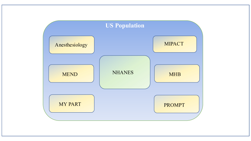
Figure 1: Figure depicts the relationship between the target population, three internal non-probability samples ($K=3$) and external probability sample. $S_{1}$, $S_{2}$, $S_{3}$ and $S_{\text{ext}}$ are the selection indicator variables of three internal and external samples respectively.

We analyze data from $K$ internal non-probability samples (cohorts) drawn from the same target population. Each cohort is represented by a binary selection indicator $S_{k}$ for $k=1,2,\ldots,K$, and we allow for overlaps among these cohorts, assuming that individual-level data can be shared across them. Figure 1 demonstrates potential overlap between the $K=3$ cohorts. The variables $\boldsymbol{Z}_{1k}$ are those that only appear in the disease model, while $\boldsymbol{Z}_{2k}$ are shared by both the disease and selection models. Across all cohorts, the covariate set $\boldsymbol{Z}$ is a union of $\boldsymbol{Z}_{1k}$ and $\boldsymbol{Z}_{2k}$, with corresponding parameter vectors $\boldsymbol{\theta}_{\boldsymbol{Z}}=(\boldsymbol{\theta}_{1k},\boldsymbol{\theta}_{2k})$. Additionally, $\boldsymbol{W}_{k}$ denotes the variables appearing exclusively in the selection model for cohort $k$. We also account for the possibility that the disease indicator $D$ may influence the selection process. The cohort-specific selection probability is given by $P(S_{k}=1|\boldsymbol{X}_{k})=\pi_{k}(\boldsymbol{X}_{k})$, where $\boldsymbol{X}_{k}$ includes $D$, $\boldsymbol{Z}_{2k}$, and $\boldsymbol{W}_{k}$. The selection mechanisms for each cohort are assumed to operate independently, conditioned on their selection variables. The composite selection indicator $S=\max(S_{1},S_{2},\ldots,S_{K})$ captures overall selection into the study sample.

Our main goal is to estimate the parameters of the conditional distribution $D|\boldsymbol{Z}$, but we can only directly assess $D|\boldsymbol{Z},S=1$ from the data. As shown by Beesley and Mukherjee (2022), the true model parameters and those from the naively fitted model (conditional on $S=1$) are related as follows:

$$\text{logit}(P(D=1|\boldsymbol{Z},S=1))=\theta_{0}+\boldsymbol{\theta}_{\boldsymbol{Z}}^{\prime}\boldsymbol{Z}+\text{log}(r(\boldsymbol{Z}))\cdot$$ (2)

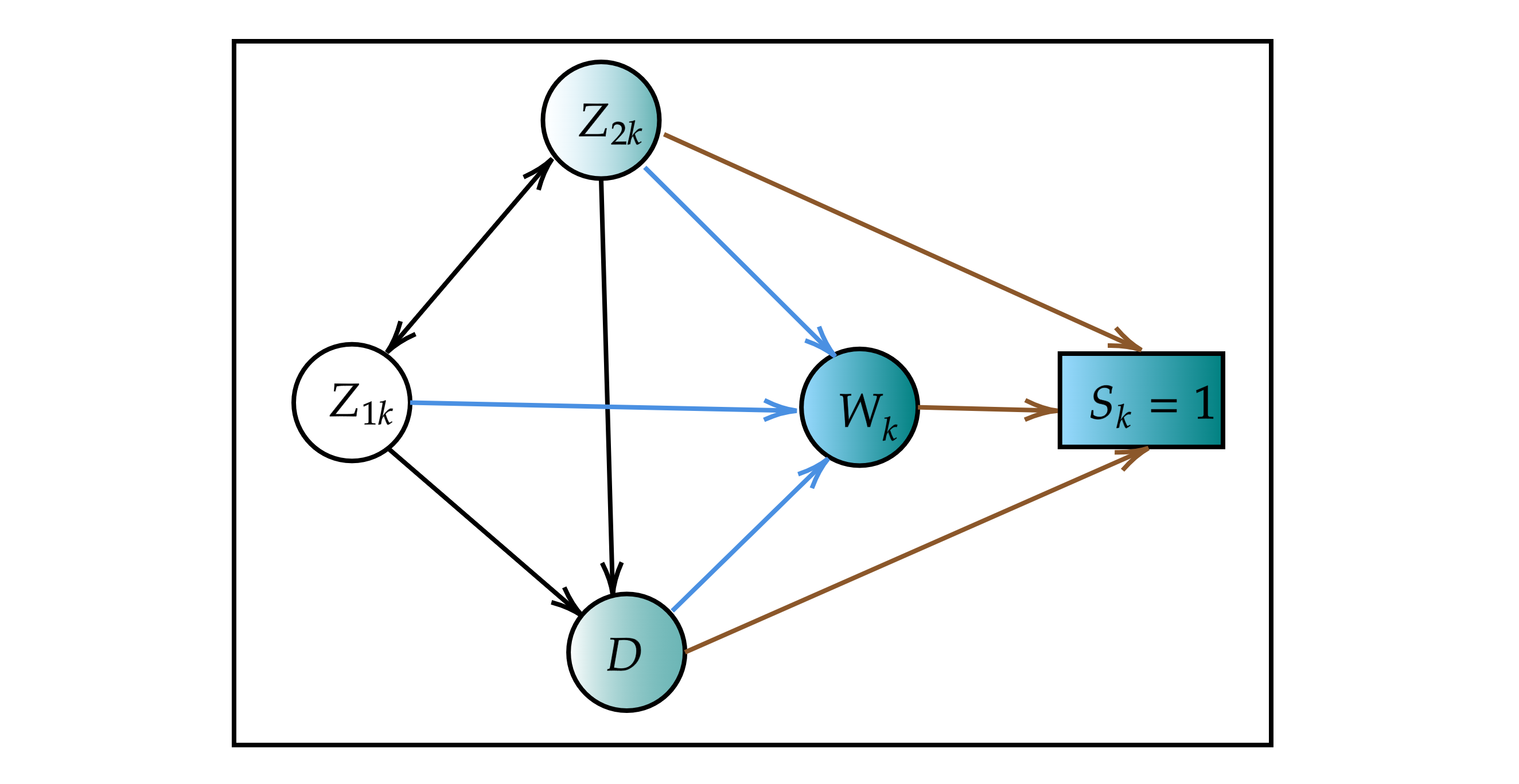
Figure 2: Selection Directed Acyclic Graphs (DAGs) representing some the most relationships between different variables of interest in internal sample $k$, where $k\in\{1,2,...,K\}$: $D$ (Disease Indicator), $S_{k}$ (Selection Indicator into the internal sample $k$), $\boldsymbol{Z}_{1k}$ (Predictors in the disease model only (White), $\boldsymbol{Z}_{2k}$ (Predictors both in disease and selection models (Mixture of Blue and White)) and $\boldsymbol{W}_{k}$ (Predictors in the selection model only (Blue)).

where $r(\boldsymbol{Z})=\frac{P(S=1|D=1,\boldsymbol{Z})}{P(S=1|D=0,\boldsymbol{Z})}$ represents how the disease model covariates $\boldsymbol{Z}$ affect the selection mechanism. Figure 2 illustrates the relationships among the disease and selection model variables through a selection DAG. While we considered the most general and complex DAG setup, in some cohorts, certain arrows may be absent and strengths of associations may vary. Unweighted logistic regression, as described in equation (2), typically leads to biased estimates of $\boldsymbol{\theta}_{\boldsymbol{Z}}$. The next section will explore methods to reduce selection bias in the context of multi-cohort analysis.

3 Framework and Methods

3.1 Joint Methods

For each individual $i$ in the target population, the combined selection probability is modeled as $\pi(\boldsymbol{X}_{i})=P(S_{i}=1\mid\boldsymbol{X}_{i})$, which represents the likelihood of being selected into at least one cohort, where $\boldsymbol{X_{i}}$ is the union of all cohort-specific selection covariates, $\boldsymbol{X_{i}}=\boldsymbol{X}_{1i}\cup\boldsymbol{X}_{2i}\cup\ldots\cup\boldsymbol{X}_{Ki}$. Assuming independent selection for each sample, conditional on $\boldsymbol{X}_{i}$, we have:

$$\pi(\boldsymbol{X}_{i}) =P(\text{max}(S_{1i},S_{2i},..,S_{Ki})=1|\boldsymbol{X}_{i})=1-P[\text{max}(S_{1i},S_{2i},..,S_{Ki})=0|\boldsymbol{X}_{i}]$$

$$=1-[1-\pi_{1}(\boldsymbol{X}_{1i})][1-\pi_{2}(\boldsymbol{X}_{2i})]...[1-\pi_{K}(\boldsymbol{X}_{Ki})]\cdot$$ (3)

With known cohort-specific selection propensity functions, $\pi_{1}(.),\pi_{2}(.),\ldots,\pi_{K}(.)$, we estimate the parameters $\boldsymbol{\theta}_{\boldsymbol{Z}}$ using a weighted logistic score equation:

$$\frac{1}{N}\sum_{i=1}^{N}\frac{S_{i}}{\pi(\boldsymbol{X}_{i})}\left\{D_{i}\boldsymbol{Z}_{i}-\frac{e^{\boldsymbol{\theta}_{\boldsymbol{Z}}^{\prime}\boldsymbol{Z}_{i}}}{(1+e^{\boldsymbol{\theta}_{\boldsymbol{Z}}^{\prime}\boldsymbol{Z}_{i}})}\boldsymbol{Z}_{i}\right\}=\mathbf{0}.$$ (4)

The consistency of the estimated parameters $\widehat{\boldsymbol{\theta}}_{\boldsymbol{Z}}$, derived from equation (4), assuming known selection probabilities $\pi(\boldsymbol{X}_{i})$, is demonstrated in supplementary section S2.1. Supplementary sections S2.2 and S2.3 provide the asymptotic distribution of $\widehat{\boldsymbol{\theta}}_{\boldsymbol{Z}}$ and a consistent estimator for the asymptotic variance, with detailed proofs.

3.2 Extension of existing IPW methods for multiple non-probability samples

For non-probability samples, selection probabilities are typically unknown, necessitating the use of two-step joint IPW approaches. This method starts with estimating selection probabilities $\widehat{\pi}(\boldsymbol{X})$. Estimation of each cohort’s individual selection probabilities $\widehat{\pi}_{1}(\boldsymbol{X}_{1})$, $\widehat{\pi}_{2}(\boldsymbol{X}_{2})$, …, and $\widehat{\pi}_{K}(\boldsymbol{X}_{K})$ using external level information, allows construction of the overall joint selection probability $\widehat{\pi}(\boldsymbol{X})$ using equation (3). Disease model parameters $\boldsymbol{\theta}_{\boldsymbol{Z}}$ are then estimated using the weighted score equation (4) where the true selection probabilities $\pi(\boldsymbol{X})$ are replaced with $\widehat{\pi}(\boldsymbol{X})$.

To estimate cohort-specific selection models, we use selection propensity estimation techniques from Kundu et al. (2024), including Pseudolikelihood (PL) (Chen et al., 2020), Simplex Regression (SR) (Beesley and Mukherjee, 2022), Post Stratification (PS) (Holt and Smith, 1979), and Calibration (CL) (Wu, 2003), extended to multi-cohort contexts and denoted by JPL, JSR, JPS, and JCL. The first two methods rely on access to individual-level data on selection variables from an external probability sample representing the target population, while the latter two rely on summary-level statistics of the selection variables. In our data analysis in Section 5, our target population of interest is the adult US population $(\text{Age}\geq 18)$, hence NHANES (National Health and Nutrition Examination Survey) data is an excellent choice for using as an external probability sample. NHANES is a complex multi-stage survey that provides a representative sample of the U.S. civilian, non-institutionalized population. It includes extensive data on health and nutrition, physical examinations, laboratory tests, demographic and socioeconomic information, and responses to health-related questionnaires.

While the details of each joint IPW method is provided in supplementary sections S3, S4, S5 and S6, we illustrate our extension approach for one of them, namely JPL here. For JPL, we first specify a parametric form for $\pi_{k}(\boldsymbol{X}_{k})$ as $\pi_{k}(\boldsymbol{X}_{k},\boldsymbol{\alpha}_{k})=\frac{e^{\boldsymbol{\alpha}_{k}^{\prime}\boldsymbol{X}_{k}}}{1+e^{\boldsymbol{\alpha}_{k}^{\prime}\boldsymbol{X}_{k}}}$, for $k=1,2,\ldots,K$. Selection parameters $\boldsymbol{\alpha}_{k}$ are estimated using the pseudolikelihood estimating equation, $\frac{1}{N}\sum_{i=1}^{N}S_{ki}\boldsymbol{X}_{ki}-\frac{1}{N}\sum_{i=1}^{N}\left(\frac{S_{\text{ext},i}}{\pi_{\text{ext},i}}\right)\pi_{k}(\boldsymbol{X}_{ki},\boldsymbol{\alpha}_{k})\boldsymbol{X}_{ki}=\mathbf{0}$, where $S_{\text{ext}}$ and $\pi_{\text{ext}}$ denote the selection indicator variable and known sampling/design probabilities for the external probability sample. The second term of this estimating equation is estimated using the information from the external data. The Newton-Raphson method is used to solve $\boldsymbol{\alpha}_{k}$ in this equation. The internal selection probabilities $\pi_{k}(\boldsymbol{X}_{ki},\boldsymbol{\alpha}_{k})$ are then estimated by plugging in estimated $\widehat{\boldsymbol{\alpha}}_{k}$ for all the cohorts. Using these probabilities and equation (3), we calculate the joint selection probability $\widehat{\pi}(\boldsymbol{X})$, which is used in the IPW equation (4) to estimate $\widehat{\boldsymbol{\theta}}_{\boldsymbol{Z}}$. Proofs of consistency, asymptotic distribution, and variance estimator for $\widehat{\boldsymbol{\theta}}_{\boldsymbol{Z}}$ under multiple selection mechanisms are detailed in supplementary section S3. Descriptions and proofs for the other three joint IPW methods are provided in supplementary sections S4, S5, and S6. However, consistent estimation of disease model parameters using joint IPW methods requires the correct specification of selection models across all $K$ cohorts, which is a challenging task in practice. Next we propose a Doubly Robust (DR) method, which estimates disease model parameters and provides robustness against misspecified selection models.

3.3 Joint Augmented Inverse Probability Weighted Method (JAIPW)

3.3.1 Motivation

The standard DR estimating equation combines a selection propensity score component with an outcome prediction model (auxiliary score model). However, when the outcome variable $D$ directly affects the selection mechanism, the traditional approach to construct the auxiliary model—based on the conditional distribution of $D|\boldsymbol{X}$—fails, as $P(D=1|\boldsymbol{X})\neq P(D=1|\boldsymbol{X},S=1)$. To address this, we identify variables in the disease model that do not directly influence selection indicators (a common subset of $\boldsymbol{Z}_{1k}$ across cohorts) and develop an auxiliary score model that leverages the relationship between this common subset of $\boldsymbol{Z}_{1k}$ and $\boldsymbol{X}$, integrating information from an external probability sample.

3.3.2 Necessary data requirement condition for constructing JAIPW estimator

Condition C1: $\boldsymbol{Z}_{1\cap}:=\boldsymbol{Z}_{11}\cap\boldsymbol{Z}_{12}\cap\ldots\cap\boldsymbol{Z}_{1K}$ is non-empty. Availability of selection variables $\boldsymbol{X}$ in both the combined internal data and external probability data.

Note that, we do not require the availability of $\boldsymbol{Z}_{1\cap}$ in the external probability sample. The idea of constructing the auxiliary score model in this case is similar to the DR estimating equation in the context of Missing at Random (MAR) literature (Williamson et al., 2012). In our scenario, the auxiliary score model is constructed on the notion that $\boldsymbol{Z}_{1\cap}$ is missing at random in the external probability sample, such as genetic information like Polygenic Risk Scores (PRS) or individual SNP level data, which are available for the MGI data but not for the NHANES data as shown in the second data example in Section 5.4.2. Even if $\boldsymbol{Z}_{1\cap}$ were available in the external probability sample, combining both the EHR and NHANES data together by leveraging an auxiliary score model for $\boldsymbol{Z}_{1\cap}$ would lead to increased efficiency as illustrated in the first data example in Section 5.4.1.

3.3.3 Construction of DR estimating equation

We state a necessary and sufficient condition for the consistency of the association parameter estimates from the proposed JAIPW method. Formally, we assume that,

Condition C2: $\ S=\max(S_{1},S_{2},\ldots,S_{K})\mathchoice{\mathrel{\hbox to0.0pt{$\displaystyle\perp$\hss}\mkern 2.0mu{\displaystyle\perp}}}{\mathrel{\hbox to0.0pt{$\textstyle\perp$\hss}\mkern 2.0mu{\textstyle\perp}}}{\mathrel{\hbox to0.0pt{$\scriptstyle\perp$\hss}\mkern 2.0mu{\scriptstyle\perp}}}{\mathrel{\hbox to0.0pt{$\scriptscriptstyle\perp$\hss}\mkern 2.0mu{\scriptscriptstyle\perp}}}\boldsymbol{Z}_{1\cap}\mid\boldsymbol{X}$ and $0<P(S=1|\boldsymbol{X})<1$.

This condition states that the composite selection indicator $S$ is conditionally independent of $\boldsymbol{Z}_{1\cap}$ given $\boldsymbol{X}$. It implies that $\boldsymbol{Z}_{1\cap}$ does not have a direct effect on the selection process once the variables, $\boldsymbol{X}$ are accounted for. From Figure 2, we observe: $\boldsymbol{Z}_{1k}\mathchoice{\mathrel{\hbox to0.0pt{$\displaystyle\perp$\hss}\mkern 2.0mu{\displaystyle\perp}}}{\mathrel{\hbox to0.0pt{$\textstyle\perp$\hss}\mkern 2.0mu{\textstyle\perp}}}{\mathrel{\hbox to0.0pt{$\scriptstyle\perp$\hss}\mkern 2.0mu{\scriptstyle\perp}}}{\mathrel{\hbox to0.0pt{$\scriptscriptstyle\perp$\hss}\mkern 2.0mu{\scriptscriptstyle\perp}}}S_{k}\mid\boldsymbol{X}_{k}\quad\forall k=1,2,\ldots,K$. Using this, we infer: $S_{k}\mathchoice{\mathrel{\hbox to0.0pt{$\displaystyle\perp$\hss}\mkern 2.0mu{\displaystyle\perp}}}{\mathrel{\hbox to0.0pt{$\textstyle\perp$\hss}\mkern 2.0mu{\textstyle\perp}}}{\mathrel{\hbox to0.0pt{$\scriptstyle\perp$\hss}\mkern 2.0mu{\scriptstyle\perp}}}{\mathrel{\hbox to0.0pt{$\scriptscriptstyle\perp$\hss}\mkern 2.0mu{\scriptscriptstyle\perp}}}\boldsymbol{Z}_{1k}\mid\boldsymbol{X}\implies S_{k}\mathchoice{\mathrel{\hbox to0.0pt{$\displaystyle\perp$\hss}\mkern 2.0mu{\displaystyle\perp}}}{\mathrel{\hbox to0.0pt{$\textstyle\perp$\hss}\mkern 2.0mu{\textstyle\perp}}}{\mathrel{\hbox to0.0pt{$\scriptstyle\perp$\hss}\mkern 2.0mu{\scriptstyle\perp}}}{\mathrel{\hbox to0.0pt{$\scriptscriptstyle\perp$\hss}\mkern 2.0mu{\scriptscriptstyle\perp}}}\boldsymbol{Z}_{1\cap}\mid\boldsymbol{X}\implies S=\max(S_{1},S_{2},\ldots,S_{K})\mathchoice{\mathrel{\hbox to0.0pt{$\displaystyle\perp$\hss}\mkern 2.0mu{\displaystyle\perp}}}{\mathrel{\hbox to0.0pt{$\textstyle\perp$\hss}\mkern 2.0mu{\textstyle\perp}}}{\mathrel{\hbox to0.0pt{$\scriptstyle\perp$\hss}\mkern 2.0mu{\scriptstyle\perp}}}{\mathrel{\hbox to0.0pt{$\scriptscriptstyle\perp$\hss}\mkern 2.0mu{\scriptscriptstyle\perp}}}\boldsymbol{Z}_{1\cap}\mid\boldsymbol{X}$. Hence condition C2 holds under the DAG configuration in Figure 2.

Let $\boldsymbol{Z}_{-1\cap}=\boldsymbol{Z}/\boldsymbol{Z}_{1\cap}$ and $\boldsymbol{W}=(\boldsymbol{W}_{1},\boldsymbol{W}_{2},\cdots,\boldsymbol{W}_{K})$. The auxiliary score model involves projecting the score function onto the Borel $\sigma$-algebra generated by $\boldsymbol{X}=(D,\boldsymbol{Z}_{-1\cap},\boldsymbol{W})$. The disease model score equation is: $\mathcal{U}(\boldsymbol{\theta}_{\boldsymbol{Z}})=D(1,\boldsymbol{Z})-\frac{e^{\theta_{0}+\boldsymbol{\theta}_{\boldsymbol{Z}}^{\prime}\boldsymbol{Z}}}{1+e^{\theta_{0}+\boldsymbol{\theta}_{\boldsymbol{Z}}^{\prime}\boldsymbol{Z}}}(1,\boldsymbol{Z})$. We denote this projection as $\mathbb{E}(\mathcal{U}(\boldsymbol{\theta}_{\boldsymbol{Z}})\mid\boldsymbol{X},S=1)=\mathbb{E}(\mathcal{U}(\boldsymbol{\theta}_{\boldsymbol{Z}})\mid\boldsymbol{X})=\boldsymbol{f}(\boldsymbol{X},\boldsymbol{\theta}_{\boldsymbol{Z}})$. The first equality holds due to condition C2. For known selection weight function $\pi(\boldsymbol{X}_{i})$ and auxiliary score function $\boldsymbol{f}(\boldsymbol{X},\boldsymbol{\theta}_{\boldsymbol{Z}})$, the DR estimating equation for $\boldsymbol{\theta}_{\boldsymbol{Z}}$ similar to the ones employed in missing data literature is:

$$\frac{1}{N}\sum_{i=1}^{N}\frac{S_{i}}{\pi(\boldsymbol{X}_{i})}(\mathcal{U}_{i}(\boldsymbol{\theta}_{\boldsymbol{Z}})-\boldsymbol{f}(\boldsymbol{X}_{i},\boldsymbol{\theta}_{\boldsymbol{Z}}))+\frac{1}{N}\sum_{i=1}^{N}\boldsymbol{f}(\boldsymbol{X}_{i},\boldsymbol{\theta}_{\boldsymbol{Z}})=\boldsymbol{0}\cdot$$ (5)

Since the second term cannot be estimated directly from available data, we replace it with $\frac{1}{N}\sum_{i=1}^{N}\frac{S_{\text{ext},i}}{\pi_{\text{ext},i}}\boldsymbol{f}(\boldsymbol{X}_{i},\theta_{\boldsymbol{Z}})$. The final proposed DR estimating equation is:

$$\frac{1}{N}\sum_{i=1}^{N}\frac{S_{i}}{\pi(\boldsymbol{X}_{i})}(\mathcal{U}_{i}(\boldsymbol{\theta}_{\boldsymbol{Z}})-\boldsymbol{f}(\boldsymbol{X}_{i},\boldsymbol{\theta}_{\boldsymbol{Z}}))+\frac{1}{N}\sum_{i=1}^{N}\frac{S_{\text{ext},i}}{\pi_{\text{ext},i}}\boldsymbol{f}(\boldsymbol{X}_{i},\boldsymbol{\theta}_{\boldsymbol{Z}})=\boldsymbol{0}\cdot$$ (6)

Special Case 1: Single Cohort: When $K=1$, the aggregate selection indicator $S=S_{1}$, $\boldsymbol{Z}_{1\cap}=Z_{1}$ and the auxiliary score model becomes $\mathbb{E}(\mathcal{U}(\boldsymbol{\theta}_{\boldsymbol{Z}})\mid\boldsymbol{X_{1}},S_{1}=1)=\mathbb{E}(\mathcal{U}(\boldsymbol{\theta}_{\boldsymbol{Z}})\mid\boldsymbol{X_{1}})=\boldsymbol{f_{1}}(\boldsymbol{X_{1}},\boldsymbol{\theta}_{\boldsymbol{Z}})$ in equation (6).

Special Case 2: Selection does not depend on disease/outcome: There are two subcases in this special case: $D\rightarrow W$ not present: In this case, all the unweighted, IPW and JAIPW methods estimate $\boldsymbol{\theta}_{\boldsymbol{Z}}$ unbiasedly. $D\rightarrow W$ present: In this case, the unweighted logistic regression would produce biased estimates of $\boldsymbol{\theta}_{\boldsymbol{Z}}$. Moreover, misspecification of the selection models would lead to biased estimates of $\boldsymbol{\theta}_{\boldsymbol{Z}}$ for all joint IPW methods when the arrow from $D$ to $W$ is present in Figure 2. The estimates from the proposed JAIPW method are consistent under these conditions when the auxiliary score model is correctly specified.

Special Case 3: No overlap across cohorts: Here, each individual in the population can belong to at most one cohort. In this case, a cohort-specific auxiliary score model can be constructed based on the relationship between the cohort-specific $\boldsymbol{Z}_{1k}$ and the selection variables $\boldsymbol{X}_{k}$. This allows for the formulation of cohort-specific doubly robust (DR) estimating equations. By summing these cohort-specific equations, we obtain the DR estimating equation for the combined sample. For an individual $i$ who is only part of cohort $k$, the composite selection indicator $S_{i}$ is simply the cohort-specific indicator $S_{ki}$. Thus, the composite selection probability $\pi(\boldsymbol{X}_{i})$ for person $i$ equals the selection probability specific to cohort $k$, $\pi_{k}(\boldsymbol{X}_{ki})$. In such cases, we can use the following DR equation instead of equation (6) to estimate $\boldsymbol{\theta}_{\boldsymbol{Z}}$ consistently:

$$\frac{1}{N}\sum_{k=1}^{K}\left[\sum_{i=1}^{N}\frac{S_{ik}}{\pi_{k}(\boldsymbol{X}_{ki})}\cdot(\mathcal{U}_{i}(\boldsymbol{\theta}_{\boldsymbol{Z}})-\boldsymbol{f}_{k}(\boldsymbol{X}_{ki},\boldsymbol{\theta}_{\boldsymbol{Z}}))+\sum_{i=1}^{N}\frac{S_{\text{ext},i}}{\pi_{\text{ext},i}}\cdot\boldsymbol{f}_{k}(\boldsymbol{X}_{ki},\boldsymbol{\theta}_{\boldsymbol{Z}})\right]=\boldsymbol{0}\cdot$$ (7)

where $\boldsymbol{f}_{k}(\boldsymbol{X}_{k},\boldsymbol{\theta}_{\boldsymbol{Z}})=\mathbb{E}(\mathcal{U}(\boldsymbol{\theta}_{\boldsymbol{Z}})\mid\boldsymbol{X}_{k},S_{k}=1)=\mathbb{E}(\mathcal{U}(\boldsymbol{\theta}_{\boldsymbol{Z}})\mid\boldsymbol{X}_{k})$. This approach allows independent modeling of the functions $\boldsymbol{f}_{1}(.),\boldsymbol{f}_{2}(.),\ldots,\boldsymbol{f}_{k}(.)$ for each cohort.

3.3.4 Estimation

The functional forms of the selection weight function $\pi(\boldsymbol{X}_{i})$ and the auxiliary score function $\boldsymbol{f}(\boldsymbol{X},\theta_{\boldsymbol{Z}})$ are rarely known a priori. Consequently, we need to estimate these functions.

Estimation of the Selection Model: We parameterize the joint selection model as $\pi(\boldsymbol{X}_{i},\boldsymbol{\alpha})$, where $\boldsymbol{\alpha}$ is estimated using the following equation:

$$\frac{1}{N}\sum_{i=1}^{N}\boldsymbol{q}(\boldsymbol{\alpha},\boldsymbol{X}_{i},S_{i},S_{\text{ext},i},\pi_{\text{ext},i})=\boldsymbol{0}.$$ (8)

Practitioners may employ either of the any one of the four joint IPW methods, JPL, JSR, JPS or JCL to estimate the function $\boldsymbol{q}(.)$.

Estimation of the Auxiliary Score Model - parametric approach: One can express:

$$\boldsymbol{f}(\boldsymbol{X},\boldsymbol{\theta}_{\boldsymbol{Z}})=\mathbb{E}(\mathcal{U}(\boldsymbol{\theta}_{\boldsymbol{Z}})\mid\boldsymbol{X})=\int_{\boldsymbol{Z}_{1\cap}}\mathcal{U}(\boldsymbol{Z}_{1\cap},\boldsymbol{\theta}_{\boldsymbol{Z}})\boldsymbol{f}(\boldsymbol{Z}_{1\cap}\mid\boldsymbol{X})d\boldsymbol{Z}_{1\cap}.$$ (9)

In this approach, we specify a parametric distribution for $\boldsymbol{Z}_{1\cap}\mid\boldsymbol{X}$ parameterized by $\boldsymbol{\gamma}$. Here $\boldsymbol{\gamma}$ is estimated from the score function based on the parametric distribution of $\boldsymbol{Z}_{1\cap}\mid\boldsymbol{X}$:

$$\frac{1}{N}\sum_{i=1}^{N}\boldsymbol{p}(\boldsymbol{\gamma},\boldsymbol{X}_{i},S_{i},\boldsymbol{Z}_{1\cap,i})=\boldsymbol{0}.$$ (10)

Once $\boldsymbol{\gamma}$ is estimated, we compute $\mathbb{E}(\mathcal{U}(\boldsymbol{\theta}_{\boldsymbol{Z}})\mid\boldsymbol{X})$ using equation (9). If integration proves overly complex due to high dimensionality, nonlinearity, or other factors, alternative strategies for approximation can be used. These may include numerical quadrature approximation or Monte Carlo methods.

Resultant DR equation: After estimating the two components, equation (6) can be expressed as:

$$\frac{1}{N}\sum_{i=1}^{N}\frac{S_{i}}{\pi(\boldsymbol{X}_{i},\widehat{\boldsymbol{\alpha}})}\left(\mathcal{U}_{i}(\boldsymbol{\theta}_{\boldsymbol{Z}})-\boldsymbol{f}(\boldsymbol{X}_{i},\widehat{\boldsymbol{\gamma}},\boldsymbol{\theta}_{\boldsymbol{Z}})\right)+\frac{1}{N}\sum_{i=1}^{N}\frac{S_{\text{ext},i}}{\pi_{\text{ext},i}}\boldsymbol{f}(\boldsymbol{X}_{i},\widehat{\boldsymbol{\gamma}},\boldsymbol{\theta}_{\boldsymbol{Z}})=\boldsymbol{0}.$$ (11)

where, $\widehat{\boldsymbol{\alpha}}$ and $\widehat{\boldsymbol{\gamma}}$ are obtained from solving equations (8) and (9) respectively.

Double Robustness Property: The following theorem demonstrates the double robustness property of the proposed estimating equation (11). Correct specification of the propensity score model means $P(S=1\mid\boldsymbol{X})=\pi(\boldsymbol{X},\boldsymbol{\alpha}^{*})$, where $\boldsymbol{\alpha}^{*}$ is the limit of in probability convergence of $\widehat{\boldsymbol{\alpha}}$, estimated from equation (8). Correct specification of the auxiliary score model means $\mathbb{E}(\mathcal{U}(\boldsymbol{\theta}_{\boldsymbol{Z}})\mid\boldsymbol{X})=\boldsymbol{f}(\boldsymbol{X},\boldsymbol{\theta}_{\boldsymbol{Z}})=\boldsymbol{f}(\boldsymbol{X},\boldsymbol{\theta}_{\boldsymbol{Z}},\boldsymbol{\gamma}^{*})$, where $\boldsymbol{\gamma}^{*}$ is the limit of in probability convergence of $\widehat{\boldsymbol{\gamma}}$, estimated from equation (10).

Theorem 3.1.

Under conditions C1 and C2 in the main text and standard regularity assumptions A1, A2, A3, A5, A6, and A10 in Supplementary Section S1 and assuming either the selection propensity model or the auxiliary score model, or both, is correctly specified, $\widehat{\boldsymbol{\theta}}_{\boldsymbol{Z}}$ estimated using equation (11) is consistent for $\boldsymbol{\theta}^{*}_{\boldsymbol{Z}}$ as $N\rightarrow\infty$.

The proof is provided in Supplementary Section S7.1. We derive the asymptotic distribution of $\widehat{\boldsymbol{\theta}}_{\boldsymbol{Z}}$ using JAIPW and the corresponding asymptotic variance estimator in Supplementary Sections S7.2 and S7.3. Evaluating the integral in equation (9) can be computationally challenging, especially with multivariate $\boldsymbol{Z}_{1\cap}$, and specifying the conditional distribution of $\boldsymbol{Z}_{1\cap}\mid\boldsymbol{X}$ parametrically can be difficult. Therefore, we offer an alternative way to model $\mathcal{U}(\boldsymbol{\theta}_{\boldsymbol{Z}})\mid\boldsymbol{X}$ directly using an assumption-lean flexible methods.

3.3.5 Non-parametric/Machine Learning approach for estimation of the auxiliary score model

For flexible modelling of auxiliary score function, we rewrite

$$\mathcal{U}(\boldsymbol{\theta}_{\boldsymbol{Z}})=D(1,\boldsymbol{Z}_{1\cap},\boldsymbol{Z}_{-1\cap})-\frac{e^{\theta_{0}+\boldsymbol{\theta}_{\boldsymbol{Z}_{1\cap}}^{\prime}\boldsymbol{Z}_{1\cap}+\boldsymbol{\theta}_{\boldsymbol{Z}_{-1\cap}}^{\prime}\boldsymbol{Z}_{-1\cap}}}{1+e^{\theta_{0}+\boldsymbol{\theta}_{\boldsymbol{Z}_{1\cap}}^{\prime}\boldsymbol{Z}_{1\cap}+\boldsymbol{\theta}_{\boldsymbol{Z}_{-1\cap}}^{\prime}\boldsymbol{Z}_{-1\cap}}}(1,\boldsymbol{Z}_{1\cap},\boldsymbol{Z}_{-1\cap})\cdot$$ (12)

We can rewrite the auxiliary score model as,

$$\mathbb{E}(\mathcal{U}(\boldsymbol{\theta}_{\boldsymbol{Z}})|\boldsymbol{X})=\boldsymbol{f}(\boldsymbol{X},\boldsymbol{\theta}_{\boldsymbol{Z}})=[f_{2}(\boldsymbol{X},\boldsymbol{\theta}_{\boldsymbol{Z}}),\boldsymbol{f}_{1}(\boldsymbol{X},\boldsymbol{\theta}_{\boldsymbol{Z}}),f_{2}(\boldsymbol{X},\boldsymbol{\theta}_{\boldsymbol{Z}})\boldsymbol{Z}_{-1\cap}]\cdot$$ (13)

where, $\boldsymbol{f}_{1}(\boldsymbol{X},\boldsymbol{\theta}_{\boldsymbol{Z}})=\mathbb{E}\left[\left.\left(D\boldsymbol{Z}_{1\cap}-D\boldsymbol{Z}_{1\cap}\frac{e^{\theta_{0}+\boldsymbol{\theta}_{\boldsymbol{Z}_{1\cap}}^{\prime}\boldsymbol{Z}_{1\cap}+\boldsymbol{\theta}_{\boldsymbol{Z}_{-1\cap}}^{\prime}\boldsymbol{Z}_{-1\cap}}}{1+e^{\theta_{0}+\boldsymbol{\theta}_{\boldsymbol{Z}_{1\cap}}^{\prime}\boldsymbol{Z}_{1\cap}+\boldsymbol{\theta}_{\boldsymbol{Z}_{-1\cap}}^{\prime}\boldsymbol{Z}_{-1\cap}}}\right)\right|\boldsymbol{X}\right]$ and $f_{2}(\boldsymbol{X},\boldsymbol{\theta}_{\boldsymbol{Z}})=\mathbb{E}\left[\left.\left(D-D\frac{e^{\theta_{0}+\boldsymbol{\theta}_{\boldsymbol{Z}_{1\cap}}\boldsymbol{Z}_{1\cap}+\boldsymbol{\theta}_{\boldsymbol{Z}_{-1\cap}}\boldsymbol{Z}_{-1\cap}}}{1+e^{\theta_{0}+\boldsymbol{\theta}_{\boldsymbol{Z}_{1\cap}}\boldsymbol{Z}_{1\cap}+\boldsymbol{\theta}_{\boldsymbol{Z}_{-1\cap}}\boldsymbol{Z}_{-1\cap}}}\right)\right|\boldsymbol{X}\right]$. For modeling of both $\boldsymbol{f}_{1}(\cdot)$ and $f_{2}(\cdot)$ it is natural to use non-parametric/machine learning algorithms, such as Random Forest or XGBoost, due to their inherent flexibility in capturing non-linear relationships and interactions. With such flexible modeling, we greatly reduce the problem of incorrect functional specification of ${U}(\boldsymbol{\theta}_{\boldsymbol{Z}})|\boldsymbol{X}$. However omitted variables in $\boldsymbol{X}$ in modeling ${U}(\boldsymbol{\theta}_{\boldsymbol{Z}})|\boldsymbol{X}$ may still lead to misspecification since the conditional independence of $\boldsymbol{Z}_{1\cap}$ and the selection indicator variable $S$ fails to hold in this case. The estimation of disease model parameters $\boldsymbol{\theta}_{\boldsymbol{Z}}$ using a sufficiently flexible auxiliary score model is outlined in Algorithm 1. The flexibility can come at a cost of increased variance/decreased efficiency relative to situations where the correct parametric form is known and fitted. We estimate the variance of $\widehat{\boldsymbol{\theta}}_{\boldsymbol{Z}}$ using a standard bootstrap method. A faster, approximate variance estimator for $\widehat{\boldsymbol{\theta}}_{\boldsymbol{Z}}$ is detailed in Supplementary Section S7.4. This estimator is derived by ignoring the variance contribution from the nuisance parameter estimation, providing a computationally efficient alternative for large datasets.

Result: Estimate of disease model parameters, $\boldsymbol{\theta}_{\boldsymbol{Z}}$

initialization :

 1. Set $\epsilon_{1}=10^{-8}$ and $\epsilon_{2}=10^{-8}$.

 2. Initial estimates $\widehat{\boldsymbol{\theta}}_{0,\boldsymbol{Z}}$ for $\boldsymbol{\theta}_{\boldsymbol{Z}}$ is obtained using unweighted logistic regression.

 3. Let $F_{1}=\frac{1}{N}\sum_{i=1}^{N}\frac{S_{i}}{\pi(\boldsymbol{X}_{i},{\boldsymbol{\alpha}})}(\mathcal{U}_{i}(\boldsymbol{\theta}_{\boldsymbol{Z}})-\boldsymbol{f}(\boldsymbol{X}_{i},\boldsymbol{\theta}_{\boldsymbol{Z}}))+\frac{1}{N}\sum_{i=1}^{N}\frac{S_{\text{ext},i}}{\pi_{\text{ext},i}}\boldsymbol{f}(\boldsymbol{X}_{i},\boldsymbol{\theta}_{\boldsymbol{Z}})$.

 4. $m=1$.

Estimating the Selection Probability/Propensity Model:

 Estimate the selection probability function $\pi(\boldsymbol{X},{\boldsymbol{\alpha}})$ using JPL, JSR, JPS or JCL.

while true do

     1. Using the initial estimate $\widehat{\boldsymbol{\theta}}_{0,\boldsymbol{Z}}$, we estimate $\widehat{\boldsymbol{f}}(.)$ with flexible non parametric or machine learning models for $\boldsymbol{f}_{1}(.)$ and $f_{2}(.)$.

   

    2. Using estimated $\widehat{\boldsymbol{f}}(.)$, we solve for $\boldsymbol{\theta}_{\boldsymbol{Z}}$ in $F_{1}=0$ and obtain the new $\widehat{\boldsymbol{\theta}}_{m,\boldsymbol{Z}}$.

     $m=m+1.$

     Continue steps 1 and 2 till convergence ($||\widehat{\boldsymbol{\theta}}_{m,\boldsymbol{Z}}-\widehat{\boldsymbol{\theta}}_{m-1,\boldsymbol{Z}}||<\epsilon_{1}$ and $||F_{1,m}-F_{1,m-1}||<\epsilon_{2}$, where $F_{1,m}$ is the value of $F_{1}$ at the $m^{\text{th}}$ iteration).

end while

return : $\widehat{\boldsymbol{\theta}}_{\boldsymbol{Z}}$ .

Algorithm 1 JAIPW-NP

3.4 Meta Analysis of IPW and AIPW methods

Meta-analysis is a standard statistical technique used to combine estimates from multiple studies with an underlying common parameter of interest. It aims to provide a more precise estimate of the estimand by pooling estimates from multiple studies. Fixed-effects and random-effects meta-analysis (Borenstein et al., 2010) are two common statistical approaches for meta analysis. In our case we only consider fixed/common effect inverse variance weighted estimators of the four IPW and the AIPW methods described above. The details for this method are provided in supplementary section S8.

4 Simulation Study

4.1 Basic Setup

We simulated a population of 50,000 individuals across $K=3$ cohorts, with three disease model covariates $\boldsymbol{Z}=(Z_{1},Z_{2},Z_{3})$. The disease outcome $D$ was generated using the logistic model: $D\mid Z_{1},Z_{2},Z_{3}\sim\text{Ber}\left(\frac{e^{\theta_{0}+\theta_{1}Z_{1}+\theta_{2}Z_{2}+\theta_{3}Z_{3}}}{1+e^{\theta_{0}+\theta_{1}Z_{1}+\theta_{2}Z_{2}+\theta_{3}Z_{3}}}\right)$, with $\theta_{0}=-2$, $\theta_{1}=0.35$, $\theta_{2}=0.45$, and $\theta_{3}=0.25$. The covariates in the disease and selection models varied by cohort, e.g., $\boldsymbol{Z}_{11}=Z_{1},\boldsymbol{Z}_{12}=(Z_{1},Z_{2}),\boldsymbol{Z}_{13}=(Z_{1},Z_{3})$, $\boldsymbol{Z}_{21}=(Z_{2},Z_{3}),\boldsymbol{Z}_{22}=Z_{3},\boldsymbol{Z}_{23}=Z_{2}$, and the selection-specific variables $W_{k}$ were simulated as conditional on $\boldsymbol{Z}$ and $D$. We examined two simulation scenarios differing in the complexity of the selection model $\pi(\boldsymbol{X})$. The first scenario included only main effects, while the second introduced interaction terms in the selection models. We evaluated both correct and incorrect specifications of the selection and auxiliary score models. In both scenarios, $S_{1}$ depended on $Z_{2},Z_{3},W_{1}$, and $D$; $S_{2}$ on $Z_{3},W_{2}$, and $D$; and $S_{3}$ on $Z_{2}$ and $W_{3}$. In the second scenario, interaction terms were added between the selection variables. We implemented unweighted logistic regression (with and without cohort-specific intercepts), all joint IPW methods, the proposed DR JAIPW with a flexible machine-learning based auxiliary score model, and meta-analysis of IPW methods. Due to computational complexity, we did not implement AIPW with meta-analysis, as the variance estimation via bootstrap essential to compute the inverse variance weighted estimator was computationally intensive for each simulation iteration. Further simulation details are available in Supplementary Section S9.1.

4.2 Assessing Robustness under Different Degrees of Model Misspecification

Selection Model: For the individual-level methods (JPL, JSR, and JAIPW), we estimated the selection model under four simulation scenarios: (1) all cohort models correctly specified, (2) one model misspecified (Cohort 3), (3) two models misspecified (Cohorts 2 and 3), and (4) all models misspecified. In Setup 1 (main effects only, no interactions), misspecification involved ignoring $D$ in the first two cohorts and $Z_{2}$ in the third. In Setup 2, all interaction terms were ignored. For JPS, we used two approaches: assuming the exact joint distribution of discretized selection variables or approximating joint probabilities using the product of marginals. For details of JPS implementation, look at Supplementary Section S9.2. The JCL model was fitted without interaction terms due to practical constraints, resulting in correct specification in Setup 1 and incorrect specification in Setup 2.

Auxiliary Score Model: In both simulation scenarios, $\boldsymbol{Z}_{1\cap}=Z_{1}$. To model the auxiliary score, we used the non-parametric JAIPW method, employing XGBoost for the auxiliary score component. This method was fitted with and without the inclusion of the disease indicator $D$, representing correct and incorrect specifications of the auxiliary score model.

4.3 Evaluation Metrics for Comparing Methods

In all simulation setups, we compared percentage relative bias, and relative mean squared error (RMSE) for $\theta_{1}$, $\theta_{2}$, and $\theta_{3}$ across two variations of unweighted logistic regression (without and with cohort specific intercepts), joint IPW methods, JAIPW, and the meta-analyzed unweighted and IPW methods. Estimated bias and percentage relative bias for a parameter $\theta$ using $\widehat{\theta}$ are defined as: $\text{Estimated Bias}(\theta,\widehat{\theta})=\left[\frac{1}{R}\sum_{r=1}^{R}(\widehat{\theta_{r}}-\theta)\right]\times 100$ and $\text{Relative Bias \%}(\theta,\widehat{\theta})=\frac{|\text{Bias}(\theta,\widehat{\theta})|}{|\theta|}\times 100$, where $\widehat{\theta_{r}}$ is the estimate of $\theta$ in the $r^{\text{th}}$ simulated dataset, $r=1,2,\ldots,R$. RMSE of $\widehat{\theta}$ with respect to the unweighted estimator without cohort-specific intercepts, $\widehat{\theta}_{\text{naive}}$ is defined as: $\text{RMSE}(\widehat{\theta},\widehat{\theta}_{\text{naive}})=\frac{\sum_{r=1}^{R}(\widehat{\theta_{r}}-\theta)^{2}}{\sum_{r=1}^{R}(\widehat{\theta}_{\text{naive,r}}-\theta)^{2}}\cdot$ To assess the performance of the variance estimators for all methods, we compared the average of estimated standard errors with the simulation-based Monte Carlo standard error estimates and further evaluated the coverage probabilities corresponding to these variance estimators.

4.4 Simulation Results

In this section, we present results for Setup 2, where both main and interaction effects are included in the selection models. Results for Setup 1 (main effects only) are provided in Supplementary Section S9.3. In both cases we consider correctly and incorrectly specified selection and auxiliary score models.

4.4.1 Parameter Estimation

Tables 1 and Supplementary Table S1 summarize results for joint and meta analyzed methods respectively from Setup 2, incorporating interaction terms into the selection model.

Unweighted Method: The unweighted logistic regression without cohort-specific intercepts showed significant relative biases, exceeding 30% for both $\theta_{2}$ and $\theta_{3}$. Including cohort-specific intercepts which may be a natural analytic strategy, further increased biases and RMSEs.

Joint IPW: With correctly specified selection models, JPL showed higher biases for $\theta_{2}$ (6.59%) and $\theta_{3}$ (4.92%) than JSR. JPL also had higher RMSEs, up to 0.97 compared to 0.35 for JSR. Biases and RMSEs increased as more selection models were misspecified. For example, in JPL, biases for $\theta_{1}$ and $\theta_{3}$ were 2 and 1.70, respectively, while in JSR they were 1.47 and 1.43. JPS with approximate joint probabilities showed high biases (48.44%) and RMSEs (2.24), and JCL struggled due to its inability to handle interactions.

JAIPW: JAIPW had similar biases to JPL and JSR when the selection models were correctly specified but had much lower RMSEs, indicating lower variance. When selection models were misspecified but the auxiliary score model was correct, JAIPW showed lower biases (1.72%, 4.94  and 6.76%) and RMSEs (0.34, 0.17, and 0.24), demonstrating robustness. We observe in this case, that JAIPW achieves up to five times lower relative bias and three times lower root mean square error (RMSE) compared to the best performing joint IPW methods under scenarios with misspecified selection models.

Meta-Analyzed IPW: Meta-analyzed PL and SR had greater biases and RMSEs than joint methods, with Meta-analyzed PL reaching an RMSE of 1.81 compared to 0.97 for JPL, even with correctly specified selection models.

4.4.2 Variance Estimation:

From Supplementary Table S2 we observe that, JPL and JSR had lower biases in standard error estimates compared to JAIPW. JAIPW achieved coverage probabilities around 0.95. JPS with exact joint probabilities had low bias but poor coverage for $\theta_{3}$ (0.25). JCL had very low coverage probabilities due to misspecification, despite low bias in standard error estimates.

4.4.3 Summary Takeaways

The individual-level IPW methods, JPL and JSR, show negligible biases when all selection models are correctly specified, with low RMSEs in the first setup (main effects only). However, in the setup with interaction terms, variance increases significantly for both methods, leading to higher RMSEs, even when selection models are correctly specified in our analysis. As more selection models are misspecified, both bias and RMSE increase for JPL and JSR. While JPL and JSR outperform JPS under correct selection model specification, JPS performs better when selection models are misspecified. JCL behaves similarly to JPL, but in the interaction scenario, JCL struggles due to reliance on marginal distribution data from the target population, causing selection model misspecification. Joint methods (JPL, JSR, JPS, and JCL) generally show lower biases and RMSEs compared to meta-analyzed counterparts, possibly due to finite sample effects.

In Setup 1, when only main effects are included in the selection model, JAIPW shows slightly higher biases and RMSEs than JPL and JSR with correct selection models due to its non-parametric auxiliary score function. However, JAIPW outperforms both in bias and RMSE when the auxiliary score model is accurate and selection models are misspecified. The benefits of JAIPW are even more evident in Setup 2, which includes interaction terms. Here, JAIPW maintains similar biases but significantly lower RMSEs than JPL and JSR when selection models are correctly specified, demonstrating its effectiveness with selection models containing interactions between the selection variables. Overall, JAIPW consistently offers reduced bias and RMSE in both setups when dealing with incorrect selection models, and it performs better than IPW methods in scenarios with interaction terms in the selection models, regardless of model specification.

5 Data Example - Multi clinic recruitment in MGI

5.1 Introduction

In this section, we use data from MGI, a large biobank that links biosamples to EHRs at the University of Michigan. Since 2012, MGI has recruited over 100,000 participants across six specialized clinics: MGI Anesthesiology, MIPACT (Michigan Predictive Activity and Clinical Trajectories), MEND (Metabolism, Endocrinology, and Diabetes), MHB2 (Mental Health BioBank), PROMPT (PROviding Mental Health Precision Treatment), and MY PART (Michigan and You – Partnering to Advance Research Together, a diverse cohort that oversamples Black, Latino/a or LatinX, Middle Eastern, and North African populations). We conduct two analyses using MGI data. For both analyses, we use NHANES 2017-18 as an external probability sample to obtain a representative data on the selection variables. The post-stratification and calibration weights were calculated using age-specific and marginal statistics from SEER (Surveillance, Epidemiology, and End Results), the U.S. Census, and the CDC (Centers for Disease Control). In the first analysis, we investigate the association between cancer ($D$) and biological sex ($Z_{1}$), both unadjusted and adjusted for age ($Z_{2}$). The unadjusted log-odds ratio is compared to benchmark SEER data (2008-2016), which show lower cancer risk for women than men, with marginal log-odds ratios ranging from -0.24 to -0.07. In the second analysis, we estimate the age-adjusted association ($Z_{2}$) between cancer ($D$) and the Polygenic Risk Scores (PRS) for having any cancer based on summary data from the UK Biobank ($Z_{1}$) (https://www.pgscatalog.org/score/PGS000356/). Unlike in Analysis 1, no external reference data (such as SEER) is available to compare method performance for estimating the association of PRS with cancer. However, this example illustrates a scenario where information on $Z_{1}$ (cancer PRS in this case) is not available from the target population or any external probability sample.

5.2 Data Descriptive Statistics

Analysis 1: For this analysis, we used data from four MGI cohorts (MGI Anesthesiology, MIPACT, MEND, MHB) collected up to August 2022. The MY PART and PROMPT cohorts were excluded due to small sample sizes, leaving a total of 80,371 participants: 69,294 from MGI Anesthesiology, 5,821 from MIPACT, 3,303 from MEND, and 1,953 from MHB. Cancer prevalence varied across cohorts: 52.2% in MGI Anesthesiology, 24.7% in MIPACT, 35.8% in MEND, and 16.8% in MHB. The distribution of biological sex was relatively consistent, except for MHB, where females comprised 62.7% of the cohort. The heterogeneity in descriptive statistics across relevant variables for each cohort is summarized in details in Table 2.

Analysis 2: In this analysis, we use genotyped MGI data from 2018, comprising 38,360 participants. The analysis employs the LASSOSUM polygenic risk score (PRS), which demonstrated the highest predictive power in previous studies (Fritsche et al., 2020). To select the tuning parameters for LASSOSUM PRS, the data were divided into training and testing sets, with parameter selection performed exclusively on the training set. To prevent overfitting, the final analysis was conducted on the testing set, which consisted of 15,291 individuals. Since this dataset is a subset of the 2018 MGI cohort, the analysis focuses on the MGI Anesthesiology cohort. The prevalence of cancer in this sample is approximately 68%.

5.3 Specifics of Model Fitting

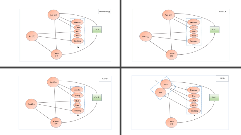
Figure 4: Directed Acyclic Graph Relationships between the disease and selection model variables in analysis of age-adjusted ($Z_{2}$) association between cancer ($D$) and biological sex ($Z_{1}$ except for MHB) in the four different cohorts of interest in the Michigan Genomics Initiative, namely MGI Anesthesiology (BB), MIPACT (Michigan Predictive Activity and Clinical Trajectories), MEND (Metabolism, Endocrinology, and Diabetes) and MHB (Mental Health BioBank). CAD, BMI, TriGly and Dep stand for Coronary Artery Disease, Body Mass Index, Triglycerides, and Depression, respectively.

Analysis 1: For each MGI cohort, distinct covariates ($\boldsymbol{W}_{K}$) were linked to different selection processes (see Figure 4). We applied the four joint IPW methods under two scenarios: one excluding and one including cancer $(D)$ in the selection models. Initially, selection weights did not account for cancer due to its low prevalence in NHANES, but an adjustment factor was later introduced, as per Kundu et al. (2024). The JAIPW method was also implemented in four forms, considering both the inclusion and exclusion of cancer in the selection and auxiliary score models. Biological sex was used as $\boldsymbol{Z}_{1\cap}$, assuming no influence on selection, except for the small MHB cohort. Biological sex was included in the MHB selection mechanism for all IPW methods and in the JAIPW model. XGBoost was used to model the conditional relationship between biological sex and other covariates in constructing the auxiliary score.

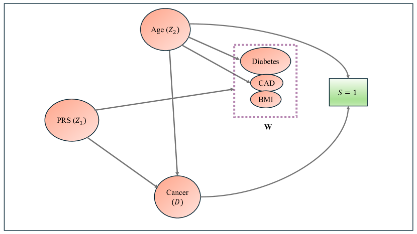
Figure S1: Directed Acyclic Graph Relationships between the disease and selection model variables in analysis of age-adjusted ($Z_{2}$) association between cancer ($D$) and Polygenic Risk Score (PRS)($Z_{1}$) for overall cancer. in the Michigan Genomics Initiative. CAD and BMI stand for Coronary Artery Disease and Body Mass Index respectively.

Analysis 2: Supplementary Figure S1 shows the DAG relationships between disease and selection variables, where PRS is the new $Z_{1}$. We constructed selection models similarly as Analysis 1 for both IPW and AIPW methods. For the auxiliary model, we tested both XGBoost and linear regression to model the relationship between Cancer PRS and the selection variables ($\boldsymbol{X}$). Since both methods produced similar results, we chose linear regression for its lower computational cost, which improved the time efficiency of variance estimation.

5.4 Results

5.4.1 Analysis 1

The benchmark national estimates from SEER shows lower lifetime cancer risk among women compared to men, with marginal log-odds ratios of -0.24 (2008-2010), -0.19 (2010-2012), -0.08 (2012-2014), and -0.07 (2014-2016). Here we present the marginal log odds ratio (OR) estimates between cancer and biological sex, with age-adjusted results in Supplementary Section S10.

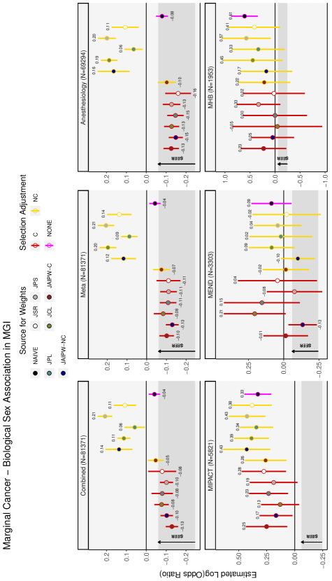
Figure 3: Estimates of the marginal association between cancer and biological sex along with 95% C.I in using JAIPW, the four joint IPW methods and the unweighted logistic regression with and without including cancer as a selection variable. The grey band represents the true SEER estimates. The red bar corresponds to the unweighted logistic method. The yellow and pink bars correspond to the estimates of the JAIPW method and the four IPW methods without and with including cancer in the selection model respectively.

MGI-Anesthesiology Subpart (C) of Figure 3 shows the results for MGI-Anesthesiology. Unweighted logistic regression estimates the log OR to be -0.08 (95% CI [-0.11, -0.05]), where the upper limit is slightly outside the SEER range. Including cancer in the selection model improved estimates for PL, SR, PS, and CL. The estimates derived from the four IPW methods— PL, SR, PS, and CL—are -0.15 (95% CI [-0.19, -0.11]), -0.16 (95% CI [-0.23, -0.10]), -0.13 (95% CI [-0.17, -0.08]), and -0.13 (95% CI [-0.17, -0.09]) respectively. Conversely, when cancer is not included in the selection model, the estimates for all methods exhibit bias in the opposite direction. For the AIPW method, estimates were -0.13 (95% CI [-0.16, -0.09]) and -0.15 (95% CI [-0.18, -0.11]) when cancer was included in both models and with inclusion/exclusion in the selection and auxiliary score model, respectively. When the selection model excluded cancer with the auxiliary score model including it, the result was -0.10 (95% CI [-0.15, -0.06]).

MIPACT: Subpart (D) of Figure 3 shows results for MIPACT. Unweighted logistic regression estimated 0.33 (95% CI [0.21, 0.45]), biased outside the SEER range. None of the IPW or AIPW estimates fell within the SEER range due to missing critical selection variables like income and education but helped to reduce the bias to some extent when cancer was included in either selection or the auxiliary score model.

MEND: Subpart (E) of Figure 3 presents results for MEND. Unweighted logistic regression estimated 0.09 (95% CI [-0.06, 0.23]). IPW methods showed bias opposite to national data, but PS yielded closer estimates (-0.08, 95% CI [-0.27, 0.12]). AIPW performed better, with mean estimates within the SEER range when the auxiliary model excluded cancer (-0.13, 95% CI [-0.24, -0.03]; -0.10, 95% CI [-0.22, 0.02]). None of the 95% CIs fully aligned with SEER data due to small sample sizes increasing variance.

MHB: Subpart (F) of Figure 3 compares methods for MHB data. Unweighted logistic regression showed high bias with an estimate of 0.61 (95% CI [0.34, 0.88]). IPW and AIPW methods reduced bias when accounting for cancer. CL with cancer included gave the closest estimate to SEER data (-0.05, 95% CI [-0.77, 0.68]). High variance in estimates, likely due to the small MHB sample size, led to wider confidence intervals and less precise estimates.

Multi Cohort: Subpart (A) of Figure 3 shows the performances of all the joint methods on the combined data. Unweighted logistic regression estimated -0.04 (95% CI [-0.07, -0.01]), outside the SEER range. Including cancer in the selection model, estimates from JPL, JSR, JPS, and JCL were -0.08 (95% CI [-0.13, -0.03]), -0.08 (95% CI [-0.15, -0.01]), -0.10 (95% CI [-0.13, -0.07]), and -0.08 (95% CI [-0.11, -0.04]), respectively. However, the upper bounds for JPL, JCL, and JSR did not align within the SEER range due to variability. Excluding cancer from the selection model led to opposite biases in estimates for all IPW methods. JAIPW estimates, when cancer was included in the selection model, had 95% CIs within the SEER range: -0.13 (95% CI [-0.16, -0.10]) and -0.10 (95% CI [-0.13, -0.07]). Excluding cancer in the selection model but including it in the auxiliary model resulted in estimates consistent with expectations, though the 95% CI did not fully align with the SEER range.

Meta Analysis: Subpart (B) of Figure 3 shows performances of the meta analyzed methods using the combined data. The results were similar to that of the joint methods on the combined data.

5.4.2 Analysis 2

Supplementary Figure S3 illustrates the age-adjusted association analysis between cancer and the cancer polygenic risk score (PRS). The unweighted method estimated a log odds ratio of 0.14 (95% CI [0.09, 0.19]) with one unit change in Interquartile Range (IQR) of PRS. In comparison, the JIPW and JAIPW methods that incorporated cancer in their models consistently produced higher point estimates compared to those excluding cancer. Notably, even when cancer was included solely in the auxiliary score model and not in the selection model, the JAIPW method estimated a log odds ratio of 0.19 (95% CI [0.09, 0.28]) with one unit change in IQR of PRS. This estimate closely aligned with those obtained from the JAIPW and JIPW methods that incorporated cancer in the selection models. These results highlight the robustness of the JAIPW method in delivering reliable estimates, comparable to those from correctly specified JIPW models, and its effectiveness in addressing potential model misspecifications.

6 Discussion

In this paper, we introduced the JAIPW method, designed to estimate disease model parameters while addressing outcome-dependent selection biases from overlapping cohorts. JAIPW shows double robustness by producing consistent estimates even when selection models are misspecified, provided an accurately specified auxiliary score model is used.

Limitations of Existing Methods: Individual-level methods like JPL and JSR struggle with misspecified selection models, while JPS and JCL are always restricted by the limited availability of summary data from external probability sample/target population. JPS fails when exact joint distributions for numerous selection variables cannot be obtained. JCL finds it challenging to specify selection models accurately using only summary statistics on the marginal distribution of the selection variables.

Advantages of JAIPW: JAIPW consistently estimates disease model parameters despite all selection models being misspecified if the auxiliary score model is correct. Simulations highlight JAIPW’s effectiveness in handling interaction terms in the functional relations between selection variables. Applying JAIPW to the MGI data on cancer and biological sex demonstrates its superiority over traditional IPW methods in cases with potential selection model inaccuracies. In applying the JAIPW method to the cancer-PRS association, we found that the method remains effective even when PRS data is unavailable in the external probability dataset.

Limitations of the JAIPW method: JAIPW’s efficiency diminishes when crucial selection variables are missing, compromising the method’s ability to adjust for selection bias fully. If key variables influencing study inclusion are absent, the assumption of conditional independence between the common variable $\boldsymbol{Z}_{1\cap}$ and the selection mechanism $S$ given $\boldsymbol{X}$ fails. Methods to assess and quantify bias, such as those by West et al. (2021) could be explored when facing missing selection variables.

Future Directions: Enhancing JAIPW robustness through more flexible modeling of the selection model, as suggested by Salvatore et al. (2024), is a potential area of extension. Wu (2022) propose a non-parametric extension of the PL method using kernel smoothing estimators. However, implementing such estimators poses significant challenges in our case of multi-dimensional selection variables. Adapting the density ratio function for estimating selection weights in data missing at random (MAR) contexts, as suggested by Wang and Kim (2021), is a potential direction. For scenarios where individual-level data cannot be shared across the cohorts, federated learning offers a privacy preserving solution. This approach, which develops models using decentralized data without exchanging individual data points, can address selection bias while respecting privacy constraints. Research by Luo and Song (2020) provides a foundation for federated learning methodologies. Future work will focus on adapting these principles to mitigate selection bias in multi-center studies where data sharing is restricted. Finally, data from EHRs is subject to numerous biases beyond selection bias, such as misclassification, missing data, clinically informative patient encounter processes, confounding, lack of consistent data harmonization across cohorts, true heterogeneity of the studied populations, and alike. Developing robust strategies to simultaneously address a confluence of biases remains a major challenge.

Code Availability

The link to the GitHub R-package EHR-MuSe can be found here, https://github.com/Ritoban1/EHR-MuSe.

Method Selection Model 1 Selection Model 2 Selection Model 3 Score Model Bias (times 100) ($\theta_{1}$) Bias (times 100) ($\theta_{2}$) Bias (times 100) ($\theta_{3}$) RMSE ($\theta_{1}$) RMSE ($\theta_{2}$) RMSE ($\theta_{3}$) Unweighted - - - - -4.94 (14.10%) 14.71 (32.67%) -7.86 (31.40%) 1 1 1 Unweighted Diff - - - - -7.82 (22.34%) -37.38 (83.07%) 5.14 (20.57%) 2.06 3.64 0.81 JSR Correct Correct Correct - -0.16 (0.47%) -0.23 (0.51%) 0.17 (0.70%) 0.35 0.04 0.15 Correct Correct Incorrect - 0.38 (1.08%) -0.49 (1.09%) 0.75 (3.01%) 0.19 0.03 0.12 Correct Incorrect Incorrect - 4.23 (12.07%) 4.79 (10.64%) 5.21 (20.83%) 0.69 0.11 0.50 Incorrect Incorrect Incorrect - 6.37 (18.19%) 6.76 (15.02%) 9.23 (36.92%) 1.47 0.22 1.43 JPL Correct Correct Correct - -0.28 (0.80%) -2.97 (6.59%) -1.23 (4.92%) 0.97 0.76 0.79 Correct Correct Incorrect - 0.47 (1.34%) -1.47 (3.26%) 0.14 (0.56%) 0.45 0.15 0.30 Correct Incorrect Incorrect - 4.93 (14.11%) 5.40 (11.99%) 5.62 (22.48%) 1.01 0.15 0.56 Incorrect Incorrect Incorrect - 7.17 (20.49%) 7.09 (15.75%) 10.33 (41.34%) 2.00 0.24 1.70 PS Actual - - - - 1.23 (3.52%) 1.00 (2.22%) 4.72 (18.89%) 0.15 0.02 0.37 PS Approx - - - - 0.41 (1.18%) -4.81 (10.68%) 12.11 (48.44%) 0.10 0.12 2.24 CL Incorrect Incorrect Incorrect - 5.59 (15.98%) 7.35 (16.32%) 8.45 (33.80%) 1.15 0.26 1.10 JAIPW Correct Correct Correct Correct 0.15 (0.43%) -2.63 (5.85%) -1.86 (7.45%) 0.47 0.21 0.35 Correct Correct Correct Incorrect -0.08 (0.23%) -3.71 (8.25%) -1.26 (5.04%) 0.84 0.88 0.82 Correct Correct Incorrect Correct -0.67 (1.92%) -2.85 (6.33%) -1.33 (5.33%) 0.47 0.18 0.31 Correct Correct Incorrect Incorrect -0.24 (0.68%) -2.52 (5.61%) 0.28 (1.14%) 0.57 0.18 0.39 Correct Incorrect Incorrect Correct 0.30 (0.84%) -2.21 (4.92%) -1.16 (4.64%) 0.34 0.16 0.21 Correct Incorrect Incorrect Incorrect 4.59 (13.10%) 3.85 (8.56%) 5.64 (22.57%) 0.92 0.09 0.58 Incorrect Incorrect Incorrect Correct 0.60 (1.72%) -2.22(4.94%) -1.69 (6.76%) 0.34 0.17 0.24 Incorrect Incorrect Incorrect Incorrect 6.97 (19.91%) 5.11 (11.36%) 9.01 (36.03%) 1.93 0.14 1.31

Table 1: Bias and RMSE Comparison between the unweighted, four joint IPW methods and JAIPW under simulation setup 2. Unweighted : Unweighted Logistic Regression, JSR : Joint Simplex Regression, JPL : Joint Pseudolikelihood, JPS : Joint Post Stratification, JCL : Joint Calibration and JAIPW : Joint Augmented Inverse Probability Weighted

Cohort Anesthesiology MIPACT MEND MHB Cancer Yes (52.2%) No (47.8%) Yes (24.7%) No (75.3%) Yes (35.8%) No (64.2%) Yes (16.8%) No (83.2%) Gender Female (53.6%) Male (46.4%) Female (53.7%) Male (46.3%) Female (51.1%) Male (48.9%) Female (62.7%) Male (37.3%) Age (Last Entry) Mean : 58.8 Sd : 16.6 Mean : 48.8 Sd : 16.7 Mean: 57.4 Sd : 16.5 Mean : 41.1 Sd : 14.7 Race Caucasian (91.0 %) Others (9.0%) Caucasian (53.4%) Others (46.5%) Caucasian (85.3%) Others (14.7%) Caucasian (88.4%) Others (11.6%) BMI Mean : 30.0 Sd : 7.2 Mean : 28.5 Sd : 7.3 Mean : 32.6 Sd : 7.8 Mean : 29.0 Sd : 7.6 CHD Yes (17.0%) No (83%) Yes (7.9%) No (92.1%) Yes (29.7%) No (70.3%) Yes (4.3%) No (95.7%) Diabetes Yes (30.9%) No (69.1%) Yes (29.8%) No (70.2%) Yes (96.2%) No (3.8%) Yes (39.6%) No (60.4%) High Trigylcerides (>=150 mg/dl) Yes (9.4%) No (90.2%) Yes (12.0%) No (88.0%) Yes (42.6%) No (57.4%) Yes (6.6%) No (93.4%) Vitamin D Deficiency (<=40) Yes (16.9%) No (83.1%) Yes (19.2%) No (80.8%) Yes (46.9%) No (53.1%) Yes (17.2%) No (82.8%) Depression Yes (32.6%) No (67.3%) Yes (27.0%) No (73.0%) Yes (44.0%) No (56.0%) Yes (81.6%) No (18.4%) Anxiety Yes (34.7%) No (65.3%) Yes (32.5%) No (67.5%) Yes (40.2%) No (59.8%) Yes (89.8%) No (10.2%)

Table 2: Descriptive Summaries of the different variables of interest in different cohorts of interest of MGI, namely Anesthesiology, MIPACT (Michigan Predictive Activity and Clinical Trajectories), MEND (Metabolism, Endocrinology, and Diabetes) and MHB (Mental Health Biobank). CHD stands for Coronary heart disease. For continuous variables we reported Mean (Sd). The definitions of phecodes have been discussed in details Supplementary Section S12.

Supplementary Section

S1 Assumptions for Proofs

A1. $\boldsymbol{\theta}^{*}_{\boldsymbol{Z}}\in\Theta$, where $\boldsymbol{\theta}^{*}_{\boldsymbol{Z}}$ is the true value of $\boldsymbol{\theta}_{\boldsymbol{Z}}$ and $\Theta$ is compact.

A2. Suppose the sample sizes of the $K$ different cohorts and the external probability sample be $n_{1},n_{2},...n_{K}$ and $n_{b}$. We assume that $n_{1},n_{2},...n_{K},n_{b}=\mathcal{O}(N)$.

A3. All the variables, including the selection indicators $S_{1},S_{2},S_{3},\cdot\cdot\cdot,S_{K}$, $D,\boldsymbol{Z}$ are considered to be random which are generally considered fixed in finite population literature.

A4. $\mathbb{E}[\sup_{\boldsymbol{\theta}\in\Theta}(G_{\boldsymbol{\theta}_{\boldsymbol{Z}}})]<\infty$ and $\mathbb{E}[\sup_{\boldsymbol{\theta}_{\boldsymbol{Z}}\in\Theta}\{\boldsymbol{g}(\boldsymbol{\theta}_{\boldsymbol{Z}})\boldsymbol{g}(\boldsymbol{\theta}_{\boldsymbol{Z}})^{\prime}\}]<\infty$.

A5. The selection model parameters $\boldsymbol{\alpha}^{*}\in\Theta_{\alpha}$ where $\Theta_{\alpha}$ is compact and $\boldsymbol{\alpha}^{*}$ is the true value of $\boldsymbol{\alpha}$

A6. Apart from the variables specified in A3, $S_{\text{ext}}$, $\boldsymbol{W}$ are also considered to be random which are generally considered fixed in finite population literature.

A7. The known external selection probability is dependent on some variables $\boldsymbol{M}$ and external selection indicators $S_{\text{ext}}$ are independent Bernoulli random variables where $P(S_{\text{ext}}=1|\boldsymbol{M})=\pi_{\text{ext}}(\boldsymbol{M})$. $\boldsymbol{M}$ can be set of any variables.

A8. Let $\eta=(\boldsymbol{\theta}_{\boldsymbol{Z}},\boldsymbol{\alpha})$ and $\mathcal{N}=\Theta\times\Theta_{\boldsymbol{\alpha}}$. Each of the following expectations are finite.

$$\mathbb{E}[\sup_{\boldsymbol{\eta}\in\mathcal{N}}(G_{\boldsymbol{\theta}_{\boldsymbol{Z}}})]<\infty\hskip 22.76228pt\mathbb{E}[\sup_{\boldsymbol{\eta}\in\mathcal{N}}(G_{\boldsymbol{\alpha}})]<\infty\hskip 22.76228pt\mathbb{E}[\sup_{\boldsymbol{\alpha}\in\Theta_{\boldsymbol{\alpha}}}(H)]<\infty$$

$$\mathbb{E}\left(\sup_{\boldsymbol{\eta}\in\mathcal{N}}\left[S\cdot\left\{\frac{1}{\pi(\boldsymbol{X},\boldsymbol{\alpha})}\right\}^{2}\left\{D-\frac{e^{\boldsymbol{\theta}_{\boldsymbol{Z}}^{\prime}\boldsymbol{Z}}}{(1+e^{\boldsymbol{\theta}_{\boldsymbol{Z}}^{\prime}\boldsymbol{Z}})}\right\}^{2}\cdot\boldsymbol{Z}\boldsymbol{Z}^{\prime}\right]\right)<\infty$$

$$\mathbb{E}\left(\sup_{\boldsymbol{\eta}\in\mathcal{N}}\left[\frac{1}{\pi(\boldsymbol{X},\boldsymbol{\alpha})}\begin{pmatrix}S_{1}\boldsymbol{X}_{1}\\ \vdots\\ S_{K}\boldsymbol{X}_{K}\\ \end{pmatrix}\cdot\left\{D\boldsymbol{Z}^{\prime}-\frac{e^{\boldsymbol{\theta}_{\boldsymbol{Z}}^{\prime}\boldsymbol{Z}}}{(1+e^{\boldsymbol{\theta}_{\boldsymbol{Z}}^{\prime}\boldsymbol{Z}})}\cdot\boldsymbol{Z}^{\prime}\right\}\right.\right.$$

$$\left.\left.-\frac{S\cdot S_{\text{ext}}}{\pi_{\text{ext}}(\boldsymbol{M})}\begin{pmatrix}\pi_{1}(\boldsymbol{X}_{1},\boldsymbol{\alpha}_{1}).\boldsymbol{X}_{1}\\ \vdots\\ \pi_{K}(\boldsymbol{X}_{K},\boldsymbol{\alpha}_{K}).\boldsymbol{X}_{K}\\ \end{pmatrix}\cdot\left\{D\boldsymbol{Z}^{\prime}-\frac{e^{\boldsymbol{\theta}_{\boldsymbol{Z}}^{\prime}\boldsymbol{Z}}}{(1+e^{\boldsymbol{\theta}_{\boldsymbol{Z}}^{\prime}\boldsymbol{Z}})}\cdot\boldsymbol{Z}^{\prime}\right\}\right]\right)<\infty$$

$$\mathbb{E}\left(\sup_{\boldsymbol{\alpha}\in\Theta_{\boldsymbol{\alpha}}}\left[\begin{pmatrix}S_{1}\boldsymbol{X}_{1}\\ \vdots\\ S_{K}\boldsymbol{X}_{K}\\ \end{pmatrix}\cdot(S_{1}\boldsymbol{X}_{1}^{\prime},\cdot\cdot\cdot,S_{K}\boldsymbol{X}_{K}^{\prime})-2S_{\text{ext}}\begin{pmatrix}\frac{\pi_{1}(\boldsymbol{X}_{1},\boldsymbol{\alpha}_{1})}{\pi_{\text{ext}}(\boldsymbol{M})}\cdot\boldsymbol{X}_{1}\\ \vdots\\ \frac{\pi_{K}(\boldsymbol{X}_{K},\boldsymbol{\alpha}_{K})}{\pi_{\text{ext}}(\boldsymbol{M})}\cdot\boldsymbol{X}_{K}\\ \end{pmatrix}\cdot(S_{1}\boldsymbol{X}_{1}^{\prime},\cdot\cdot\cdot,S_{K}\boldsymbol{X}_{K}^{\prime})\right.\right.$$

$$\left.\left.+S_{\text{ext}}\cdot\left\{\frac{1}{\pi_{\text{ext}}(\boldsymbol{M})}\right\}^{2}\cdot\begin{pmatrix}\frac{\pi_{1}(\boldsymbol{X}_{1},\boldsymbol{\alpha}_{1})}{\pi_{\text{ext}}(\boldsymbol{M})}\cdot\boldsymbol{X}_{1}\\ \vdots\\ \frac{\pi_{K}(\boldsymbol{X}_{K},\boldsymbol{\alpha}_{K})}{\pi_{\text{ext}}(\boldsymbol{M})}\cdot\boldsymbol{X}_{K}\\ \end{pmatrix}\left\{\frac{\pi_{1}(\boldsymbol{X}_{1},\boldsymbol{\alpha}_{1})}{\pi_{\text{ext}}(\boldsymbol{M})}\cdot\boldsymbol{X}_{1}^{\prime},\cdot\cdot\cdot,\frac{\pi_{K}(\boldsymbol{X}_{K},\boldsymbol{\alpha}_{K})}{\pi_{\text{ext}}(\boldsymbol{M})}\cdot\boldsymbol{X}_{K}^{\prime}\right\}\right]\right)<\infty\cdot$$

A9. Each of the following expectations are finite.

$$\mathbb{E}[\sup_{\boldsymbol{\eta}\in\mathcal{N}}(G_{\boldsymbol{\theta}_{\boldsymbol{Z}}})]<\infty\hskip 22.76228pt\mathbb{E}[\sup_{\boldsymbol{\eta}\in\mathcal{N}}(G_{\boldsymbol{\alpha}})]<\infty\hskip 22.76228pt\mathbb{E}[\sup_{\boldsymbol{\alpha}\in\Theta_{\boldsymbol{\alpha}}}(H)]<\infty$$

$$\mathbb{E}\left(\sup_{\boldsymbol{\eta}\in\mathcal{N}}\left[S\cdot\left\{\frac{1}{\pi(\boldsymbol{X},\boldsymbol{\alpha})}\right\}^{2}\left\{D-\frac{e^{\boldsymbol{\theta}_{\boldsymbol{Z}}^{\prime}\boldsymbol{Z}}}{(1+e^{\boldsymbol{\theta}_{\boldsymbol{Z}}^{\prime}\boldsymbol{Z}})}\right\}^{2}\cdot\boldsymbol{Z}\boldsymbol{Z}^{\prime}\right]\right)<\infty$$

$$\mathbb{E}\left(\sup_{\boldsymbol{\eta}\in\mathcal{N}}\left[\frac{1}{\pi(\boldsymbol{X},\boldsymbol{\alpha})}\begin{pmatrix}\frac{S_{1}\boldsymbol{X}_{1}}{\pi_{1}(\boldsymbol{X}_{1},\boldsymbol{\alpha}_{1})}\\ \vdots\\ \frac{S_{K}\boldsymbol{X}_{K}}{\pi_{K}(\boldsymbol{X}_{K},\boldsymbol{\alpha}_{K})}\\ \end{pmatrix}\cdot\left\{D\boldsymbol{Z}^{\prime}-\frac{e^{\boldsymbol{\theta}_{\boldsymbol{Z}}^{\prime}\boldsymbol{Z}}}{(1+e^{\boldsymbol{\theta}_{\boldsymbol{Z}}^{\prime}\boldsymbol{Z}})}\cdot\boldsymbol{Z}^{\prime}\right\}\right.\right.$$

$$\left.\left.-S\begin{pmatrix}\boldsymbol{X}_{1}\\ \vdots\\ \boldsymbol{X}_{K}\end{pmatrix}\cdot\left\{D\boldsymbol{Z}^{\prime}-\frac{e^{\boldsymbol{\theta}_{\boldsymbol{Z}}^{\prime}\boldsymbol{Z}}}{(1+e^{\boldsymbol{\theta}_{\boldsymbol{Z}}^{\prime}\boldsymbol{Z}})}\cdot\boldsymbol{Z}^{\prime}\right\}\right]\right)<\infty$$

$$\mathbb{E}\left(\sup_{\boldsymbol{\alpha}\in\Theta_{\boldsymbol{\alpha}}}\left[\begin{pmatrix}\frac{S_{1}\boldsymbol{X}_{1}}{\pi_{1}(\boldsymbol{X}_{1},\boldsymbol{\alpha}_{1})}\\ \vdots\\ \frac{S_{K}\boldsymbol{X}_{K}}{\pi_{K}(\boldsymbol{X}_{K},\boldsymbol{\alpha}_{K})}\\ \end{pmatrix}\cdot\left(\frac{S_{1}\boldsymbol{X}_{1}^{\prime}}{\pi_{1}(\boldsymbol{X}_{1},\boldsymbol{\alpha}_{1})},\cdot\cdot\cdot,\frac{S_{K}\boldsymbol{X}_{K}^{\prime}}{\pi_{K}(\boldsymbol{X}_{K},\boldsymbol{\alpha}_{K})}\right)\right.\right.$$

$$\left.\left.-2\begin{pmatrix}\boldsymbol{X}_{1}\\ \vdots\\ \boldsymbol{X}_{K}\\ \end{pmatrix}\cdot\left(\frac{S_{1}\boldsymbol{X}_{1}^{\prime}}{\pi_{1}(\boldsymbol{X}_{1},\boldsymbol{\alpha}_{1})},\cdot\cdot\cdot,\frac{S_{K}\boldsymbol{X}_{K}^{\prime}}{\pi_{K}(\boldsymbol{X}_{K},\boldsymbol{\alpha}_{K})}\right).+\begin{pmatrix}\boldsymbol{X}_{1}\\ \vdots\\ \boldsymbol{X}_{K}\\ \end{pmatrix}(\boldsymbol{X}_{1}^{\prime},\cdot\cdot\cdot,\boldsymbol{X}_{K}^{\prime})\right]\right)<\infty\cdot$$

A10. The auxiliary score model parameters $\boldsymbol{\gamma}^{*}\in\Theta_{\gamma}$ where $\Theta_{\gamma}$ is compact and $\boldsymbol{\gamma}^{*}$ is the true value of $\boldsymbol{\gamma}$

A11. Let $\eta=(\boldsymbol{\theta}_{\boldsymbol{Z}},\boldsymbol{\alpha},\boldsymbol{\gamma})$ and $\mathcal{N}=\Theta\times\Theta_{\boldsymbol{\alpha}}\times\Theta_{\boldsymbol{\gamma}}$. We follow the notations in Theorem SS7.1. Each of the following expectations are finite.

$$\mathbb{E}[\sup_{\boldsymbol{\eta}\in\mathcal{N}}(G_{\boldsymbol{\theta}_{\boldsymbol{Z}}})]<\infty\hskip 22.76228pt\mathbb{E}[\sup_{\boldsymbol{\eta}\in\mathcal{N}}(G_{\boldsymbol{\alpha},\boldsymbol{\gamma}})]<\infty\hskip 22.76228pt\mathbb{E}\left[\sup_{(\boldsymbol{\alpha},\boldsymbol{\gamma})\in\Theta_{\boldsymbol{\alpha}}\times\Theta_{\boldsymbol{\gamma}}}(H)\right]<\infty$$

$$\mathbb{E}\left[\sup_{\boldsymbol{\eta}\in\mathcal{N}}\left\{\boldsymbol{g}(\boldsymbol{\theta}_{\boldsymbol{Z}},\boldsymbol{\alpha},\boldsymbol{\gamma})\cdot g(\boldsymbol{\theta}_{\boldsymbol{Z}},\boldsymbol{\alpha},\boldsymbol{\gamma})^{\prime}\right\}\right]<\infty$$

$$\mathbb{E}\left[\sup_{\boldsymbol{\eta}\in\mathcal{N}}\left\{\boldsymbol{g}(\boldsymbol{\theta}_{\boldsymbol{Z}},\boldsymbol{\alpha},\boldsymbol{\gamma})\cdot\boldsymbol{h}(\boldsymbol{X},\boldsymbol{Z}_{1\cap},\boldsymbol{M},\boldsymbol{\alpha},\boldsymbol{\gamma})^{\prime}\right\}\right]<\infty$$

$$\mathbb{E}\left[\sup_{(\boldsymbol{\alpha},\boldsymbol{\gamma})\in\Theta_{\boldsymbol{\alpha}}\times\Theta_{\boldsymbol{\gamma}}}\left\{\boldsymbol{h}(\boldsymbol{X},\boldsymbol{Z}_{1\cap},\boldsymbol{M},\boldsymbol{\alpha},\boldsymbol{\gamma})\cdot\boldsymbol{h}(\boldsymbol{X},\boldsymbol{Z}_{1\cap},\boldsymbol{M},\boldsymbol{\alpha},\boldsymbol{\gamma})^{\prime}\right\}\right]<\infty\cdot$$

S2 Known Selection Probabilities

S2.1 Theorem S1

Theorem S2.1.

Under assumptions A1, A2 and A3 in Supplementary Section S1 if $\pi_{1}(.)$, $\pi_{2}(.)$, …, $\pi_{K}(.)$ are known for each individual in the target population, $\widehat{\boldsymbol{\theta}}_{\boldsymbol{Z}}$ estimated from the following weighted logistic regression estimating equation is consistent for $\theta^{*}_{\boldsymbol{Z}}$, where $\theta^{*}_{\boldsymbol{Z}}$ is the true value of $\theta_{\boldsymbol{Z}}$ satisfying equation (1) of the main text.

$$\frac{1}{N}\sum_{i=1}^{N}\frac{S_{i}}{\pi(\boldsymbol{X}_{i})}\left\{D_{i}\boldsymbol{Z}_{i}-\frac{e^{\boldsymbol{\theta}_{\boldsymbol{Z}}^{\prime}\boldsymbol{Z}_{i}}}{(1+e^{\boldsymbol{\theta}_{\boldsymbol{Z}}^{\prime}\boldsymbol{Z}_{i}})}\cdot\boldsymbol{Z}_{i}\right\}=\mathbf{0}.$$ (S1)

Proof.

Let

$$\phi_{N}(\boldsymbol{\theta}_{\boldsymbol{Z}})=\frac{1}{N}\sum_{i=1}^{N}\frac{S_{i}}{\pi(\boldsymbol{X}_{i})}\left\{D_{i}\boldsymbol{Z}_{i}-\frac{e^{\boldsymbol{\theta}_{\boldsymbol{Z}}^{\prime}\boldsymbol{Z}_{i}}}{(1+e^{\boldsymbol{\theta}_{\boldsymbol{Z}}^{\prime}\boldsymbol{Z}_{i}})}\cdot\boldsymbol{Z}_{i}\right\}\cdot$$

From Tsiatis (2006), under assumptions A1, A2 and A3 in Supplementary Section S1 it is enough to show that $\mathbb{E}(\phi_{N}(\boldsymbol{\theta}^{*}_{\boldsymbol{Z}}))=0$, in order to prove that $\widehat{\boldsymbol{\theta}_{\boldsymbol{Z}}}\xrightarrow{p}\boldsymbol{\theta}^{*}_{\boldsymbol{Z}}$, where $\widehat{\boldsymbol{\theta}_{\boldsymbol{Z}}}$ is obtained from solving $\phi_{N}(\boldsymbol{\theta}_{\boldsymbol{Z}})=\mathbf{0}$.

$$\mathbb{E}[\phi_{N}(\boldsymbol{\theta}^{*}_{\boldsymbol{Z}})] =\mathbb{E}\left[\frac{1}{N}\sum_{i=1}^{N}\frac{S_{i}}{\pi(\boldsymbol{X}_{i})}\left\{D_{i}\boldsymbol{Z}_{i}-\frac{e^{\boldsymbol{\theta}_{\boldsymbol{Z}}^{*^{\prime}}\boldsymbol{Z}_{i}}}{(1+e^{\boldsymbol{\theta}_{\boldsymbol{Z}}^{*^{\prime}}\boldsymbol{Z}_{i}})}\cdot\boldsymbol{Z}_{i}\right\}\right]$$

$$=\frac{1}{N}\sum_{i=1}^{N}\mathbb{E}\left[\frac{S_{i}}{\pi(\boldsymbol{X}_{i})}\left\{D_{i}\boldsymbol{Z}_{i}-\frac{e^{\boldsymbol{\theta}_{\boldsymbol{Z}}^{\prime}\boldsymbol{Z}_{i}}}{(1+e^{\boldsymbol{\theta}_{\boldsymbol{Z}}^{*^{\prime}}\boldsymbol{Z}_{i}})}\cdot\boldsymbol{Z}_{i}\right\}\right]$$

$$=\frac{1}{N}\sum_{i=1}^{N}\mathbb{E}_{\boldsymbol{X}_{i},\boldsymbol{Z}_{1\cap,i}}\left[\mathbb{E}\left\{\frac{S_{i}}{\pi(\boldsymbol{X}_{i})}\left.\left(D_{i}\boldsymbol{Z}_{i}-\frac{e^{\boldsymbol{\theta}_{\boldsymbol{Z}}^{*^{\prime}}\boldsymbol{Z}_{i}}}{(1+e^{\boldsymbol{\theta}_{\boldsymbol{Z}}^{*^{\prime}}\boldsymbol{Z}_{i}})}\cdot\boldsymbol{Z}_{i}\right)\right|\boldsymbol{X}_{i},\boldsymbol{Z}_{1\cap,i}\right\}\right]$$

$$=\frac{1}{N}\sum_{i=1}^{N}\mathbb{E}_{\boldsymbol{X}_{i},\boldsymbol{Z}_{1\cap,i}}\left[\left\{D_{i}\boldsymbol{Z}_{i}-\frac{e^{\boldsymbol{\theta}_{\boldsymbol{Z}}^{*^{\prime}}\boldsymbol{Z}_{i}}}{(1+e^{\boldsymbol{\theta}_{\boldsymbol{Z}}^{*^{\prime}}\boldsymbol{Z}_{i}})}\cdot\boldsymbol{Z}_{i}\right\}\cdot\frac{1}{\pi(\boldsymbol{X}_{i})}\mathbb{E}\left(S_{i}|\boldsymbol{X}_{i},\boldsymbol{Z}_{1\cap,i}\right)\right]\cdot$$

Using equation (5) of the main text we obtain that $\mathbb{E}(S|\boldsymbol{X},\boldsymbol{Z}_{1\cap})=\mathbb{E}(S|\boldsymbol{X})=\pi(\boldsymbol{X})$. Hence we obtain

$$\mathbb{E}[\phi_{N}(\boldsymbol{\theta}^{*}_{\boldsymbol{Z}})]=\frac{1}{N}\sum_{i=1}^{N}\mathbb{E}_{\boldsymbol{X}_{i},\boldsymbol{Z}_{1\cap,i}}\left\{D_{i}\boldsymbol{Z}_{i}-\frac{e^{\boldsymbol{\theta}_{\boldsymbol{Z}}^{*^{\prime}}\boldsymbol{Z}_{i}}}{(1+e^{\boldsymbol{\theta}_{\boldsymbol{Z}}^{*^{\prime}}\boldsymbol{Z}_{i}})}\cdot\boldsymbol{Z}_{i}\right\}$$

$$=\frac{1}{N}\sum_{i=1}^{N}\mathbb{E}_{D_{i},\boldsymbol{Z}_{i}}\left\{D_{i}\boldsymbol{Z}_{i}-\frac{e^{\boldsymbol{\theta}_{\boldsymbol{Z}}^{*^{\prime}}\boldsymbol{Z}_{i}}}{(1+e^{\boldsymbol{\theta}_{\boldsymbol{Z}}^{*^{\prime}}\boldsymbol{Z}_{i}})}\cdot\boldsymbol{Z}_{i}\right\}$$

$$=\frac{1}{N}\sum_{i=1}^{N}\mathbb{E}_{\boldsymbol{z}_{i}}\left[\mathbb{E}\left\{\left.\left(D_{i}\boldsymbol{Z}_{i}-\frac{e^{\boldsymbol{\theta}_{\boldsymbol{Z}}^{*^{\prime}}\boldsymbol{Z}_{i}}}{(1+e^{\boldsymbol{\theta}_{\boldsymbol{Z}}^{*^{\prime}}\boldsymbol{Z}_{i}})}\cdot\boldsymbol{Z}_{i}\right)\right|\boldsymbol{Z}_{i}\right\}\right]$$

$$=\frac{1}{N}\sum_{i=1}^{N}\mathbb{E}\left\{\frac{e^{\boldsymbol{\theta}_{\boldsymbol{Z}}^{*^{\prime}}\boldsymbol{Z}_{i}}}{(1+e^{\boldsymbol{\theta}_{\boldsymbol{Z}}^{*^{\prime}}\boldsymbol{Z}_{i}})}\cdot\boldsymbol{Z}_{i}-\frac{e^{\boldsymbol{\theta}_{\boldsymbol{Z}}^{*^{\prime}}\boldsymbol{Z}_{i}}}{(1+e^{\boldsymbol{\theta}_{\boldsymbol{Z}}^{*^{\prime}}\boldsymbol{Z}_{i}})}\cdot\boldsymbol{Z}_{i}\right\}=\mathbf{0}\cdot$$

The last step is obtained from the relation between $D$ and $\boldsymbol{Z}$ given by equation (1) of the main text. ∎

S2.2 Theorem S2

Theorem S2.2.

Under assumptions of Theorem S1 when the selection weights are known and we do not take into consideration estimation of selection model parameter, the asymptotic distribution of $\widehat{\boldsymbol{\theta}}_{\boldsymbol{Z}}$ is given by

$$\sqrt{N}(\widehat{\boldsymbol{\theta}_{\boldsymbol{Z}}}-\boldsymbol{\theta}^{*}_{\boldsymbol{Z}})\xrightarrow{d}\mathcal{N}(0,V)\hskip 14.22636pt\text{as}\hskip 14.22636ptN\rightarrow\infty\cdot$$

where

$$V=(G_{\boldsymbol{\theta}_{\boldsymbol{Z}}^{*}})^{-1}\cdot\mathbb{E}[\boldsymbol{g}\cdot\boldsymbol{g}^{\prime}]\cdot(G_{\boldsymbol{\theta}_{\boldsymbol{Z}}^{*}}^{-1})^{{}^{\prime}}\hskip 22.76228ptG_{\boldsymbol{\theta}_{\boldsymbol{Z}}^{*}}=\mathbb{E}\left\{-\frac{S}{\pi(\boldsymbol{X})}\cdot\frac{e^{\boldsymbol{\theta}_{\boldsymbol{Z}}^{*^{\prime}}\boldsymbol{Z}}}{(1+e^{\boldsymbol{\theta}_{\boldsymbol{Z}}^{*^{\prime}}\boldsymbol{Z}})^{2}}\cdot\boldsymbol{Z}\boldsymbol{Z}^{\prime}\right\}$$

$$\boldsymbol{g}(\boldsymbol{\theta}_{\boldsymbol{Z}}^{*})=\frac{S}{\pi(\boldsymbol{X})}\left\{D\boldsymbol{Z}-\frac{e^{\boldsymbol{\theta}_{\boldsymbol{Z}}^{*^{\prime}}\boldsymbol{Z}}}{(1+e^{\boldsymbol{\theta}_{\boldsymbol{Z}}^{*^{\prime}}\boldsymbol{Z}})}\cdot\boldsymbol{Z}\right\}\cdot$$

Proof.

By Tsiatis (2006)’s arguments for a Z-estimation problem under assumptions of Theorem S1 we obtain

$$\sqrt{N}(\widehat{\boldsymbol{\theta}_{\boldsymbol{Z}}}-\boldsymbol{\theta}^{*}_{\boldsymbol{Z}})\xrightarrow{d}\mathcal{N}(0,V)\hskip 14.22636pt\text{as}\hskip 14.22636ptN\rightarrow\infty\cdot$$

where

$$V=(G_{\boldsymbol{\theta}_{\boldsymbol{Z}}^{*}})^{-1}\cdot\mathbb{E}[\boldsymbol{g}\cdot\boldsymbol{g}^{\prime}]\cdot(G_{\boldsymbol{\theta}_{\boldsymbol{Z}}^{*}}^{-1})^{{}^{\prime}}\hskip 22.76228ptG_{\boldsymbol{\theta}_{\boldsymbol{Z}}^{*}}=\left.\mathbb{E}\left\{\frac{\partial g(\boldsymbol{\theta}_{\boldsymbol{Z}}^{*})}{\partial\boldsymbol{\theta}_{\boldsymbol{Z}}}\right\}\right|_{\boldsymbol{\theta}=\boldsymbol{\theta}_{\boldsymbol{Z}}^{*}}$$

$$\boldsymbol{g}(\boldsymbol{\theta}_{\boldsymbol{Z}}^{*})=\frac{S}{\pi(\boldsymbol{X})}\left\{D\boldsymbol{Z}-\frac{e^{\boldsymbol{\theta}_{\boldsymbol{Z}}^{*^{\prime}}\boldsymbol{Z}}}{(1+e^{\boldsymbol{\theta}_{\boldsymbol{Z}}^{*^{\prime}}\boldsymbol{Z}})}\cdot\boldsymbol{Z}\right\}\cdot$$

This proof just requires the calculation of $G_{\boldsymbol{\theta}_{\boldsymbol{Z}}^{*}}$.

Calculation for $G_{\boldsymbol{\theta}_{\boldsymbol{Z}}^{*}}$

$$\left.\frac{\partial\boldsymbol{g}(\boldsymbol{\theta}_{\boldsymbol{Z}})}{\partial\boldsymbol{\theta}_{\boldsymbol{Z}}}\right|_{\boldsymbol{\theta}_{\boldsymbol{Z}}=\boldsymbol{\theta}_{\boldsymbol{Z}}^{*}}=\left.\frac{\partial}{\partial\boldsymbol{\theta}_{\boldsymbol{Z}}}\left[\frac{S}{\pi(\boldsymbol{X})}\left\{D\boldsymbol{Z}-\frac{e^{\boldsymbol{\theta}_{\boldsymbol{Z}}^{*^{\prime}}\boldsymbol{Z}}}{(1+e^{\boldsymbol{\theta}_{\boldsymbol{Z}}^{*^{\prime}}\boldsymbol{Z}})}\cdot\boldsymbol{Z}\right\}\right]\right|_{\boldsymbol{\theta}_{\boldsymbol{Z}}=\boldsymbol{\theta}_{\boldsymbol{Z}}^{*}}$$

$$=-\frac{S}{\pi(\boldsymbol{X})}\cdot\frac{e^{\boldsymbol{\theta}_{\boldsymbol{Z}}^{*^{\prime}}\boldsymbol{Z}}}{(1+e^{\boldsymbol{\theta}_{\boldsymbol{Z}}^{*^{\prime}}\boldsymbol{Z}})^{2}}\cdot\boldsymbol{Z}\boldsymbol{Z}^{\prime}$$

Therefore we obtain

$$G_{\boldsymbol{\theta}_{\boldsymbol{Z}}^{*}}=\mathbb{E}\left\{-\frac{S}{\pi(\boldsymbol{X})}\cdot\frac{e^{\boldsymbol{\theta}_{\boldsymbol{Z}}^{*^{\prime}}\boldsymbol{Z}}}{(1+e^{\boldsymbol{\theta}_{\boldsymbol{Z}}^{*^{\prime}}\boldsymbol{Z}})^{2}}\cdot\boldsymbol{Z}\boldsymbol{Z}^{\prime}\right\}\cdot$$

∎

S2.3 Theorem S3

Theorem S2.3.

Under assumptions A1, A2, A3 and A4, $\frac{1}{N}\cdot\widehat{G_{\boldsymbol{\theta}_{\boldsymbol{Z}}}}^{-1}\cdot\widehat{E}\cdot(\widehat{G_{\boldsymbol{\theta}_{\boldsymbol{Z}}}}^{-1})^{{}^{\prime}}$ is a consistent estimator of the asymptotic variance of $\widehat{\boldsymbol{\theta}}_{\boldsymbol{Z}}$ where

$$\widehat{G_{\boldsymbol{\theta}_{\boldsymbol{Z}}}}=\frac{1}{N}\sum_{i=1}^{N}\left\{\frac{S_{i}}{\pi(\boldsymbol{X}_{i})}\cdot\frac{e^{\widehat{\boldsymbol{\theta}_{\boldsymbol{Z}}}^{\prime}\boldsymbol{Z}_{i}}}{(1+e^{\widehat{\boldsymbol{\theta}_{\boldsymbol{Z}}}^{\prime}\boldsymbol{Z}_{i}})^{2}}\cdot\boldsymbol{Z}_{i}\boldsymbol{Z}_{i}^{\prime}\right\}\cdot$$

$$\widehat{E}=\frac{1}{N}\sum_{i=1}^{N}S_{i}\cdot\left\{\frac{1}{\pi(\boldsymbol{X}_{i})}\right\}^{2}\left\{D_{i}-\frac{e^{\widehat{\boldsymbol{\theta}_{\boldsymbol{Z}}}^{\prime}\boldsymbol{Z}_{i}}}{(1+e^{\widehat{\boldsymbol{\theta}}^{\prime}\boldsymbol{Z}_{i}})}\right\}^{2}\cdot\boldsymbol{Z}_{i}\boldsymbol{Z}_{i}^{\prime}\cdot$$

Proof.

First we prove that as $N\rightarrow\infty$

$$\frac{1}{N}\sum_{i=1}^{N}\left\{\frac{S_{i}}{\pi(\boldsymbol{X}_{i})}\cdot\frac{e^{\widehat{\boldsymbol{\theta}_{\boldsymbol{Z}}}^{\prime}\boldsymbol{Z}_{i}}}{(1+e^{\widehat{\boldsymbol{\theta}_{\boldsymbol{Z}}}^{\prime}\boldsymbol{Z}_{i}})^{2}}\cdot\boldsymbol{Z}_{i}\boldsymbol{Z}_{i}^{\prime}\right\}\xrightarrow{p}\mathbb{E}\left\{\frac{S}{\pi(\boldsymbol{X})}\cdot\frac{e^{\boldsymbol{\theta}_{\boldsymbol{Z}}^{*^{\prime}}\boldsymbol{Z}}}{(1+e^{\boldsymbol{\theta}_{\boldsymbol{Z}}^{*^{\prime}}\boldsymbol{Z}})^{2}}\cdot\boldsymbol{Z}\boldsymbol{Z}^{\prime}\right\}\cdot$$

Using assumptions A1, A2, A3 and A4 and Uniform Law of Large Numbers (ULLN), we obtain

$$\sup_{\boldsymbol{\theta}_{\boldsymbol{Z}}\in\Theta}\left|\left|\frac{1}{N}\sum_{i=1}^{N}\left\{\frac{S_{i}}{\pi(\boldsymbol{X}_{i})}\cdot\frac{e^{\boldsymbol{\theta}_{\boldsymbol{Z}}^{\prime}\boldsymbol{Z}_{i}}}{(1+e^{\boldsymbol{\theta}_{\boldsymbol{Z}}^{\prime}\boldsymbol{Z}_{i}})^{2}}\cdot\boldsymbol{Z}_{i}\boldsymbol{Z}_{i}^{\prime}\right\}-\mathbb{E}\left\{\frac{S}{\pi(\boldsymbol{X})}\cdot\frac{e^{\boldsymbol{\theta}_{\boldsymbol{Z}}^{{}^{\prime}}\boldsymbol{Z}}}{(1+e^{\boldsymbol{\theta}_{\boldsymbol{Z}}^{{}^{\prime}}\boldsymbol{Z}})^{2}}\cdot\boldsymbol{Z}\boldsymbol{Z}^{\prime}\right\}\right|\right|\xrightarrow{p}\mathbf{0}\cdot$$ (S2)

Since this above expression holds for any $\boldsymbol{\theta}_{\boldsymbol{Z}}\in\Theta$, therefore it is true for $\widehat{\boldsymbol{\theta}}_{\boldsymbol{Z}}$. This implies

$$\left|\left|\frac{1}{N}\sum_{i=1}^{N}\left.\left\{\frac{S_{i}}{\pi(\boldsymbol{X}_{i})}\cdot\frac{e^{\widehat{\boldsymbol{\theta}_{\boldsymbol{Z}}}^{\prime}\boldsymbol{Z}_{i}}}{(1+e^{\widehat{\boldsymbol{\theta}_{\boldsymbol{Z}}}^{\prime}\boldsymbol{Z}_{i}})^{2}}\cdot\boldsymbol{Z}_{i}\boldsymbol{Z}_{i}^{\prime}\right\}-\mathbb{E}\left\{\frac{S}{\pi(\boldsymbol{X})}\cdot\frac{e^{\boldsymbol{\theta}_{\boldsymbol{Z}}^{{}^{\prime}}\boldsymbol{Z}}}{(1+e^{\boldsymbol{\theta}_{\boldsymbol{Z}}^{{}^{\prime}}\boldsymbol{Z}})^{2}}\cdot\boldsymbol{Z}\boldsymbol{Z}^{\prime}\right\}\right|_{\boldsymbol{\theta}_{\boldsymbol{Z}}=\widehat{\boldsymbol{\theta}_{\boldsymbol{Z}}}}\right|\right|\xrightarrow{p}\mathbf{0}\cdot$$ (S3)

Using Triangle Inequality we obtain

$$\left|\left|\frac{1}{N}\sum_{i=1}^{N}\left\{\frac{S_{i}}{\pi(\boldsymbol{X}_{i})}\cdot\frac{e^{\widehat{\boldsymbol{\theta}_{\boldsymbol{Z}}}^{\prime}\boldsymbol{Z}_{i}}}{(1+e^{\boldsymbol{\theta}_{\boldsymbol{Z}}^{\prime}\boldsymbol{Z}_{i}})^{2}}\cdot\boldsymbol{Z}_{i}\boldsymbol{Z}_{i}^{\prime}\right\}-\mathbb{E}\left\{\frac{S}{\pi(\boldsymbol{X})}\cdot\frac{e^{\boldsymbol{\theta}_{\boldsymbol{Z}}^{*^{\prime}}\boldsymbol{Z}}}{(1+e^{\boldsymbol{\theta}_{\boldsymbol{Z}}^{*^{\prime}}\boldsymbol{Z}})^{2}}\cdot\boldsymbol{Z}\boldsymbol{Z}^{\prime}\right\}\right|\right|\leq$$ (S4)

$$\left|\left|\frac{1}{N}\sum_{i=1}^{N}\left.\left\{\frac{S_{i}}{\pi(\boldsymbol{X}_{i})}\cdot\frac{e^{\widehat{\boldsymbol{\theta}_{\boldsymbol{Z}}}^{\prime}\boldsymbol{Z}_{i}}}{(1+e^{\widehat{\boldsymbol{\theta}_{\boldsymbol{Z}}}^{\prime}\boldsymbol{Z}_{i}})^{2}}\cdot\boldsymbol{Z}_{i}\boldsymbol{Z}_{i}^{\prime}\right\}-\mathbb{E}\left\{\frac{S}{\pi(\boldsymbol{X})}\cdot\frac{e^{\boldsymbol{\theta}_{\boldsymbol{Z}}^{{}^{\prime}}\boldsymbol{Z}}}{(1+e^{\boldsymbol{\theta}_{\boldsymbol{Z}}^{{}^{\prime}}\boldsymbol{Z}})^{2}}\cdot\boldsymbol{Z}\boldsymbol{Z}^{\prime}\right\}\right|_{\boldsymbol{\theta}_{\boldsymbol{Z}}=\widehat{\boldsymbol{\theta}_{\boldsymbol{Z}}}}\right|\right|+$$ (S5)

$$\left.\left|\left|\mathbb{E}\left\{\frac{S}{\pi(\boldsymbol{X})}\cdot\frac{e^{\boldsymbol{\theta}_{\boldsymbol{Z}}^{{}^{\prime}}\boldsymbol{Z}}}{(1+e^{\boldsymbol{\theta}_{\boldsymbol{Z}}^{{}^{\prime}}\boldsymbol{Z}})^{2}}\cdot\boldsymbol{Z}\boldsymbol{Z}^{\prime}\right\}\right|_{\boldsymbol{\theta}_{\boldsymbol{Z}}=\widehat{\boldsymbol{\theta}_{\boldsymbol{Z}}}}-\mathbb{E}\left\{\frac{S}{\pi(\boldsymbol{X})}\cdot\frac{e^{\boldsymbol{\theta}_{\boldsymbol{Z}}^{*^{\prime}}\boldsymbol{Z}}}{(1+e^{\boldsymbol{\theta}_{\boldsymbol{Z}}^{*^{\prime}}\boldsymbol{Z}})^{2}}\cdot\boldsymbol{Z}\boldsymbol{Z}^{\prime}\right\}\right|\right|\cdot$$ (S6)

Since we proved that $\widehat{\boldsymbol{\theta}_{\boldsymbol{Z}}}\xrightarrow{p}\boldsymbol{\theta}_{\boldsymbol{Z}}^{*}$ in Theorem S1, therefore by Continuous Mapping Theorem

$$\left.\left|\left|\mathbb{E}\left\{\frac{S}{\pi(\boldsymbol{X})}\cdot\frac{e^{\boldsymbol{\theta}_{\boldsymbol{Z}}^{{}^{\prime}}\boldsymbol{Z}}}{(1+e^{\boldsymbol{\theta}_{\boldsymbol{Z}}^{{}^{\prime}}\boldsymbol{Z}})^{2}}\cdot\boldsymbol{Z}\boldsymbol{Z}^{\prime}\right\}\right|_{\boldsymbol{\theta}_{\boldsymbol{Z}}=\widehat{\boldsymbol{\theta}_{\boldsymbol{Z}}}}-\mathbb{E}\left\{\frac{S}{\pi(\boldsymbol{X})}\cdot\frac{e^{\boldsymbol{\theta}_{\boldsymbol{Z}}^{*^{\prime}}\boldsymbol{Z}}}{(1+e^{\boldsymbol{\theta}_{\boldsymbol{Z}}^{*^{\prime}}\boldsymbol{Z}})^{2}}\cdot\boldsymbol{Z}\boldsymbol{Z}^{\prime}\right\}\right|\right|\xrightarrow{p}\mathbf{0}\cdot$$ (S7)

Using equations (S3), (S4), (S5), (S6) and (S7) we obtain

$$\frac{1}{N}\sum_{i=1}^{N}\left\{\frac{S_{i}}{\pi(\boldsymbol{X}_{i})}\cdot\frac{e^{\widehat{\boldsymbol{\theta}_{\boldsymbol{Z}}}^{\prime}\boldsymbol{Z}_{i}}}{(1+e^{\widehat{\boldsymbol{\theta}_{\boldsymbol{Z}}}^{\prime}\boldsymbol{Z}_{i}})^{2}}\cdot\boldsymbol{Z}_{i}\boldsymbol{Z}_{i}^{\prime}\right\}\xrightarrow{p}\mathbb{E}\left\{\frac{S}{\pi(\boldsymbol{X})}\cdot\frac{e^{\boldsymbol{\theta}_{\boldsymbol{Z}}^{*^{\prime}}\boldsymbol{Z}}}{(1+e^{\boldsymbol{\theta}_{\boldsymbol{Z}}^{*^{\prime}}\boldsymbol{Z}})^{2}}\cdot\boldsymbol{Z}\boldsymbol{Z}^{\prime}\right\}\cdot$$

Therefore we obtain

$$-\widehat{G_{\boldsymbol{\theta}_{\boldsymbol{Z}}}}\xrightarrow{p}-G_{\boldsymbol{\theta}_{\boldsymbol{Z}}^{*}}\hskip 14.22636pt\text{which implies}\hskip 14.22636pt\widehat{G_{\boldsymbol{\theta}_{\boldsymbol{Z}}}}\xrightarrow{p}G_{\boldsymbol{\theta}_{\boldsymbol{Z}}^{*}}\cdot$$

Using the exact same set of arguments we obtain

$$\widehat{E}=\frac{1}{N}\sum_{i=1}^{N}S_{i}\cdot\left\{\frac{1}{\pi(\boldsymbol{X}_{i})}\right\}^{2}\left\{D_{i}-\frac{e^{\widehat{\boldsymbol{\theta}_{\boldsymbol{Z}}}^{\prime}\cdot\boldsymbol{Z}_{i}}}{(1+e^{\hat{\theta}^{\prime}\cdot\boldsymbol{Z}_{i}})}\right\}^{2}\cdot\boldsymbol{Z}_{i}\boldsymbol{Z}_{i}^{\prime}$$

$$\xrightarrow{p}\mathbb{E}[\boldsymbol{g}(\boldsymbol{\theta}_{\boldsymbol{Z}}^{*})\cdot\boldsymbol{g}(\boldsymbol{\theta}_{\boldsymbol{Z}}^{*})^{\prime}]=\mathbb{E}\left[S\cdot\left\{\frac{1}{\pi(\boldsymbol{X})}\right\}^{2}\cdot\left\{D-\frac{e^{\boldsymbol{\theta}_{\boldsymbol{Z}}^{*^{\prime}}\boldsymbol{Z}}}{(1+e^{\boldsymbol{\theta}_{\boldsymbol{Z}}^{*^{\prime}}\boldsymbol{Z}})}\right\}^{2}\cdot\boldsymbol{Z}\boldsymbol{Z}^{\prime}\right]\cdot$$

Combining together the consistency of $\widehat{G_{\boldsymbol{\theta}_{\boldsymbol{Z}}}}$ and $\widehat{E}$ we obtain

$$\widehat{V}=\widehat{G_{\boldsymbol{\theta}_{\boldsymbol{Z}}}}^{-1}\cdot\widehat{E}\cdot(\widehat{G_{\boldsymbol{\theta}_{\boldsymbol{Z}}}}^{-1})^{{}^{\prime}}\xrightarrow{p}V=(G_{\boldsymbol{\theta}_{\boldsymbol{Z}}^{*}})^{-1}\cdot\mathbb{E}[g(\boldsymbol{\theta}_{\boldsymbol{Z}}^{*})\cdot\boldsymbol{g}(\boldsymbol{\theta}_{\boldsymbol{Z}}^{*})^{\prime}].(G_{\boldsymbol{\theta}_{\boldsymbol{Z}}^{*}}^{-1})^{{}^{\prime}}\cdot$$

From Theorem S2.2 $$\sqrt{N}(\widehat{\boldsymbol{\theta}_{\boldsymbol{Z}}}-\boldsymbol{\theta}_{\boldsymbol{Z}}^{*})\xrightarrow{d}\mathcal{N}\{0,(G_{\boldsymbol{\theta}_{\boldsymbol{Z}}^{*}})^{-1}\cdot\mathbb{E}[g(\boldsymbol{\theta}_{\boldsymbol{Z}}^{*})\cdot\boldsymbol{g}(\boldsymbol{\theta}_{\boldsymbol{Z}}^{*})^{\prime}]\cdot(G_{\boldsymbol{\theta}_{\boldsymbol{Z}}^{*}}^{-1})^{{}^{\prime}}\}$$

Therefore we obtain

$$\text{Var}\{\sqrt{N}(\widehat{\boldsymbol{\theta}_{\boldsymbol{Z}}}-\boldsymbol{\theta}_{\boldsymbol{Z}}^{*})\}=(G_{\boldsymbol{\theta}_{\boldsymbol{Z}}^{*}})^{-1}\cdot\mathbb{E}[g(\boldsymbol{\theta}_{\boldsymbol{Z}}^{*})\cdot\boldsymbol{g}(\boldsymbol{\theta}_{\boldsymbol{Z}}^{*})^{\prime}]\cdot(G_{\boldsymbol{\theta}_{\boldsymbol{Z}}^{*}}^{-1})^{{}^{\prime}}+O_{p}(1)$$

$$N\cdot\text{Var}(\widehat{\boldsymbol{\theta}_{\boldsymbol{Z}}})=(G_{\boldsymbol{\theta}_{\boldsymbol{Z}}^{*}})^{-1}\cdot\mathbb{E}[g(\boldsymbol{\theta}_{\boldsymbol{Z}}^{*})\cdot\boldsymbol{g}(\boldsymbol{\theta}_{\boldsymbol{Z}}^{*})^{\prime}]\cdot(G_{\boldsymbol{\theta}_{\boldsymbol{Z}}^{*}}^{-1})^{{}^{\prime}}+O_{p}(1)$$

$$\text{Var}(\widehat{\boldsymbol{\theta}_{\boldsymbol{Z}}})=\frac{1}{N}\cdot(G_{\boldsymbol{\theta}_{\boldsymbol{Z}}^{*}})^{-1}\cdot\mathbb{E}[g(\boldsymbol{\theta}_{\boldsymbol{Z}}^{*})\cdot\boldsymbol{g}(\boldsymbol{\theta}_{\boldsymbol{Z}}^{*})^{\prime}]\cdot(G_{\boldsymbol{\theta}_{\boldsymbol{Z}}^{*}}^{-1})^{{}^{\prime}}+O_{p}\left(\frac{1}{N}\right)$$

$$\text{Var}(\widehat{\boldsymbol{\theta}_{\boldsymbol{Z}}})=\frac{1}{N}\cdot\widehat{G_{\boldsymbol{\theta}_{\boldsymbol{Z}}}}^{-1}\cdot\widehat{E}\cdot(\widehat{G_{\boldsymbol{\theta}_{\boldsymbol{Z}}}}^{-1})^{{}^{\prime}}+o_{p}\left(1\right)=\frac{\widehat{V}}{N}+o_{p}\left(1\right)\cdot$$

Therefore $\frac{\widehat{V}}{N}$ is a consistent estimator of asymptotic variance of $\widehat{\boldsymbol{\theta}}_{\boldsymbol{Z}}$. ∎

S3 Joint Pseudolikelihood-based Estimating equation (JPL)

S3.1 Theorem S4

Theorem S3.1.

Under assumptions A1, A2 A5, A6 and A7 in Supplementary Section S1 and assuming the selection model is correctly specified, that is, $\pi(\boldsymbol{X},\boldsymbol{\alpha}^{*})=P(S=1|\boldsymbol{X})=\pi(\boldsymbol{X})$ where $\widehat{\boldsymbol{\alpha}}\xrightarrow{p}\boldsymbol{\alpha}^{*}$ and $\boldsymbol{\alpha}^{*}$ is the true value of $\boldsymbol{\alpha}$, then $\widehat{\boldsymbol{\theta}}_{\boldsymbol{Z}}$ estimated using JPL is consistent for $\boldsymbol{\theta}_{\boldsymbol{Z}}^{*}$ as $N\rightarrow\infty$.

Proof.

In this case, the estimating equation consists of both selection model and disease model parameter estimation. The two step estimating equation is given by

$$\delta_{n}(\boldsymbol{\alpha})=\begin{pmatrix}\delta_{1_{n}}(\boldsymbol{\alpha}_{1})=\frac{1}{N}\sum_{i=1}^{N}S_{1i}\boldsymbol{X}_{1i}-\frac{1}{N}\cdot\sum_{i=1}^{N}\left(\frac{S_{\text{ext},i}}{\pi_{\text{ext},i}}\right)\cdot\pi_{k}(\boldsymbol{X}_{1i},\boldsymbol{\alpha}_{1})\cdot\boldsymbol{X}_{1i}\\ \vdots\\ \delta_{K_{n}}(\boldsymbol{\alpha}_{K})=\frac{1}{N}\sum_{i=1}^{N}S_{Ki}\boldsymbol{X}_{Ki}-\frac{1}{N}\cdot\sum_{i=1}^{N}\left(\frac{S_{\text{ext},i}}{\pi_{\text{ext},i}}\right)\cdot\pi_{k}(\boldsymbol{X}_{Ki},\boldsymbol{\alpha}_{K})\cdot\boldsymbol{X}_{Ki}\\ \end{pmatrix}$$

$$\phi_{n}(\boldsymbol{\theta}_{\boldsymbol{Z}},\widehat{\boldsymbol{\alpha}})=\frac{1}{N}\sum_{i=1}^{N}\frac{S_{i}}{\pi(\boldsymbol{X}_{i},\widehat{\boldsymbol{\alpha}})}\left\{D_{i}\boldsymbol{Z}_{i}-\frac{e^{\boldsymbol{\theta}^{\prime}\boldsymbol{Z}_{i}}}{(1+e^{\boldsymbol{\theta}^{\prime}\boldsymbol{Z}_{i}})}\cdot\boldsymbol{Z}_{i}\right\}\cdot$$

From Tsiatis (2006) to show $\widehat{\boldsymbol{\theta}_{\boldsymbol{Z}}}\xrightarrow{p}\boldsymbol{\theta}_{\boldsymbol{Z}}^{*}$ in a two step estimation procedure, we need to prove $\mathbb{E}(\phi_{N}(\boldsymbol{\theta}_{\boldsymbol{Z}}^{*},\boldsymbol{\alpha}^{*}))=\mathbf{0}$. Under correct specification of selection model, $\pi(\boldsymbol{X},\boldsymbol{\alpha}^{*})=P(S=1|\boldsymbol{X})=\pi(\boldsymbol{X})$ wwhere $\widehat{\boldsymbol{\alpha}}\xrightarrow{p}\boldsymbol{\alpha}^{*}$ and $\boldsymbol{\alpha}^{*}$ is the true value of $\boldsymbol{\alpha}$. Using this equality, the proof to show that $\mathbb{E}(\phi_{N}(\boldsymbol{\theta}_{\boldsymbol{Z}}^{*},\boldsymbol{\alpha}^{*}))=\mathbf{0}$ is exactly as Theorem S1. Therefore we obtain $\widehat{\boldsymbol{\theta}}_{\boldsymbol{Z}}$ is a consistent estimator of $\boldsymbol{\theta}_{\boldsymbol{Z}}^{*}$. ∎

S3.2 Theorem S5

Theorem S3.2.

Under assumptions of Theorem S4 and suppose $\widehat{\boldsymbol{\theta}_{\boldsymbol{Z}}}\xrightarrow{p}\boldsymbol{\theta}_{\boldsymbol{Z}}^{*}$, the asymptotic distribution of $\widehat{\boldsymbol{\theta}}_{\boldsymbol{Z}}$ using JPL is given by

$$\sqrt{N}(\widehat{\boldsymbol{\theta}_{\boldsymbol{Z}}}-\boldsymbol{\theta}^{*}_{\boldsymbol{Z}})\xrightarrow{d}\mathcal{N}(\mathbf{0},V).$$ (S8)

where

$$V=(G_{\boldsymbol{\theta}_{\boldsymbol{Z}}^{*}})^{-1}.\mathbb{E}[\{\boldsymbol{g}(\boldsymbol{\theta}_{\boldsymbol{Z}}^{*},\boldsymbol{\alpha}^{*})+G_{\boldsymbol{\alpha}^{*}}.\boldsymbol{\Psi}(\boldsymbol{\alpha}^{*})\}\{\boldsymbol{g}(\boldsymbol{\theta}_{\boldsymbol{Z}}^{*},\boldsymbol{\alpha}^{*})+G_{\boldsymbol{\alpha}^{*}}.\boldsymbol{\Psi}(\boldsymbol{\alpha}^{*})\}^{\prime}].(G_{\boldsymbol{\theta}_{\boldsymbol{Z}}^{*}}^{-1})^{{}^{\prime}}$$

$$G_{\boldsymbol{\theta}_{\boldsymbol{Z}}^{*}}=\mathbb{E}\left\{-\frac{S}{\pi(\boldsymbol{X},\boldsymbol{\alpha}^{*})}\cdot\frac{e^{\boldsymbol{\theta}_{\boldsymbol{Z}}^{*^{\prime}}\boldsymbol{Z}}}{(1+e^{\boldsymbol{\theta}_{\boldsymbol{Z}}^{*^{\prime}}\boldsymbol{Z}})^{2}}\cdot\boldsymbol{Z}\boldsymbol{Z}^{\prime}\right\}$$

$$\boldsymbol{g}(\boldsymbol{\theta}_{\boldsymbol{Z}}^{*},\boldsymbol{\alpha}^{*})=\frac{S}{\pi(\boldsymbol{X},\boldsymbol{\alpha}^{*})}\left\{D\boldsymbol{Z}-\frac{e^{\boldsymbol{\theta}_{\boldsymbol{Z}}^{*^{\prime}}\boldsymbol{Z}}}{(1+e^{\boldsymbol{\theta}_{\boldsymbol{Z}}^{*^{\prime}}\boldsymbol{Z}})}\cdot\boldsymbol{Z}\right\}$$

$$G_{\boldsymbol{\alpha}^{*}}=\mathbb{E}\left[-\frac{S}{\pi(\boldsymbol{X},\boldsymbol{\alpha}^{*})^{2}}.\{1-\pi_{1}(\boldsymbol{X}_{1},\boldsymbol{\alpha}^{*}_{1})\}\cdot\cdot\cdot\{1-\pi_{K}(\boldsymbol{X}_{K},\boldsymbol{\alpha}^{*}_{K})\}\cdot\right.$$

$$\hskip 56.9055pt\left.\boldsymbol{Z}\cdot\{\pi_{1}(\boldsymbol{X}_{1},\boldsymbol{\alpha}_{1}^{*})\cdot\boldsymbol{X}_{1}^{\prime},\cdot\cdot\cdot,\pi_{K}(\boldsymbol{X}_{K},\boldsymbol{\alpha}^{*}_{K})\cdot\boldsymbol{X}_{K}^{\prime}\}\cdot\left\{D-\frac{e^{\boldsymbol{\theta}_{\boldsymbol{Z}}^{*^{\prime}}\boldsymbol{Z}}}{(1+e^{\boldsymbol{\theta}_{\boldsymbol{Z}}^{*^{\prime}}\boldsymbol{Z}})}\right\}\right]$$

$$\boldsymbol{h}(\boldsymbol{X},\boldsymbol{M},\boldsymbol{\alpha}^{*})=\begin{pmatrix}S_{1}\boldsymbol{X}_{1}-\frac{\pi_{1}(\boldsymbol{X}_{1},\boldsymbol{\alpha}^{*}_{1})}{\pi_{\text{ext}}(\boldsymbol{M})}\cdot S_{\text{ext}}\cdot\boldsymbol{X}_{1}\\ \vdots\\ S_{K}\boldsymbol{X}_{K}-\frac{\pi_{1}(\boldsymbol{X}_{K},\boldsymbol{\alpha}^{*}_{K})}{\pi_{\text{ext}}(\boldsymbol{M})}\cdot S_{\text{ext}}\cdot\boldsymbol{X}_{K}\\ \end{pmatrix}$$

$$H=-\mathbb{E}\begin{pmatrix}\frac{\pi_{1}(\boldsymbol{X}_{1},\boldsymbol{\alpha}^{*}_{1})}{\pi_{\text{ext}}(\boldsymbol{M})}\cdot\{1-\pi_{1}(\boldsymbol{X}_{1},\boldsymbol{\alpha}^{*}_{1})\}\cdot S_{\text{ext}}\cdot\boldsymbol{X}_{1}\boldsymbol{X}_{1}^{\prime}&\ldots&0\\ \vdots&\ddots&\vdots\\ 0&\ldots&\frac{\pi_{K}(\boldsymbol{X}_{K},\boldsymbol{\alpha}^{*}_{K})}{\pi_{\text{ext}}(\boldsymbol{M})}\cdot\{1-\pi_{K}(\boldsymbol{X}_{K},\boldsymbol{\alpha}^{*}_{K})\}\cdot S_{\text{ext}}\cdot\boldsymbol{X}_{K}\boldsymbol{X}_{K}^{\prime}\end{pmatrix}$$

$$\boldsymbol{\Psi}(\boldsymbol{\alpha}^{*})=-H^{-1}\cdot\boldsymbol{h}(\boldsymbol{X},\boldsymbol{M},\boldsymbol{\alpha}^{*})$$

Proof.

By Tsiatis (2006)’s arguments on a two step Z-estimation problem, under assumptions of Theorem S4 and since $\widehat{\boldsymbol{\theta}_{\boldsymbol{Z}}}\xrightarrow{p}\boldsymbol{\theta}_{\boldsymbol{Z}}^{*}$, we obtain that

$$\sqrt{N}(\widehat{\boldsymbol{\theta}_{\boldsymbol{Z}}}-\boldsymbol{\theta}_{\boldsymbol{Z}}^{*})\xrightarrow{d}\mathcal{N}(0,(G_{\boldsymbol{\theta}_{\boldsymbol{Z}}^{*}})^{-1}.\mathbb{E}[\{\boldsymbol{g}(\boldsymbol{\theta}_{\boldsymbol{Z}}^{*},\boldsymbol{\alpha}^{*})+G_{\boldsymbol{\alpha}^{*}}.\boldsymbol{\Psi}(\boldsymbol{\alpha}^{*})\}\{\boldsymbol{g}(\boldsymbol{\theta}_{\boldsymbol{Z}}^{*},\boldsymbol{\alpha}^{*})+G_{\boldsymbol{\alpha}^{*}}.\boldsymbol{\Psi}(\boldsymbol{\alpha}^{*})\}^{\prime}].(G_{\boldsymbol{\theta}_{\boldsymbol{Z}}^{*}}^{-1})^{{}^{\prime}}\cdot$$

We derive the expression of each of the terms in the above expression.

$$G_{\boldsymbol{\theta}_{\boldsymbol{Z}}^{*}}=\left.\mathbb{E}\left\{\frac{\partial g(\boldsymbol{\theta}_{\boldsymbol{Z}},\boldsymbol{\alpha}^{*})}{\partial\boldsymbol{\theta}_{\boldsymbol{Z}}}\right\}\right|_{\boldsymbol{\theta}_{\boldsymbol{Z}}=\boldsymbol{\theta}_{\boldsymbol{Z}}^{*}}\hskip 28.45274pt\left.G_{\boldsymbol{\alpha}^{*}}=\mathbb{E}\left\{\frac{\partial g(\boldsymbol{\theta}_{\boldsymbol{Z}}^{*},\boldsymbol{\alpha})}{\partial\boldsymbol{\alpha}}\right\}\right|_{\boldsymbol{\alpha}=\boldsymbol{\alpha}^{*}}$$

$$H=\left.\mathbb{E}\left\{\frac{\partial\boldsymbol{h}(\boldsymbol{\alpha})}{\partial\boldsymbol{\alpha}}\right\}\right|_{\boldsymbol{\alpha}=\boldsymbol{\alpha}^{*}}\hskip 54.06006pt\boldsymbol{\Psi}(\boldsymbol{\alpha}^{*})=-H^{-1}\boldsymbol{h}(\boldsymbol{\alpha}^{*})\cdot$$

First we calculate $G_{\boldsymbol{\theta}_{\boldsymbol{Z}}^{*}}$.

Calculation for $G_{\boldsymbol{\theta}_{\boldsymbol{Z}}^{*}}$

$$\left.\frac{\partial\boldsymbol{g}(\boldsymbol{\theta}_{\boldsymbol{Z}},\boldsymbol{\alpha}^{*})}{\partial\boldsymbol{\theta}_{\boldsymbol{Z}}}\right|_{\boldsymbol{\theta}_{\boldsymbol{Z}}=\boldsymbol{\theta}_{\boldsymbol{Z}}^{*}}=\left.\frac{\partial}{\partial\boldsymbol{\theta}_{\boldsymbol{Z}}}\left[\frac{S}{\pi(\boldsymbol{X},\boldsymbol{\alpha}^{*})}\left\{D\boldsymbol{Z}-\frac{e^{\boldsymbol{\theta}_{\boldsymbol{Z}}^{*^{\prime}}\boldsymbol{Z}}}{(1+e^{\boldsymbol{\theta}_{\boldsymbol{Z}}^{*^{\prime}}\boldsymbol{Z}})}\cdot\boldsymbol{Z}\right\}\right]\right|_{\boldsymbol{\theta}_{\boldsymbol{Z}}=\boldsymbol{\theta}_{\boldsymbol{Z}}^{*}}$$

$$=-\frac{S}{\pi(\boldsymbol{X},\boldsymbol{\alpha}^{*})}\cdot\frac{e^{\boldsymbol{\theta}_{\boldsymbol{Z}}^{*^{\prime}}\boldsymbol{Z}}}{(1+e^{\boldsymbol{\theta}_{\boldsymbol{Z}}^{*^{\prime}}\boldsymbol{Z}})^{2}}\cdot\boldsymbol{Z}\boldsymbol{Z}^{\prime}\cdot$$

Therefore we obtain

$$G_{\boldsymbol{\theta}_{\boldsymbol{Z}}^{*}}=\mathbb{E}\left[-\frac{S}{\pi(\boldsymbol{X},\boldsymbol{\alpha}^{*})}\cdot\frac{e^{\boldsymbol{\theta}_{\boldsymbol{Z}}^{*^{\prime}}\boldsymbol{Z}}}{(1+e^{\boldsymbol{\theta}_{\boldsymbol{Z}}^{*^{\prime}}\boldsymbol{Z}})^{2}}\cdot\boldsymbol{Z}\boldsymbol{Z}^{\prime}\right]\cdot$$

Next we calculate $G_{\boldsymbol{\alpha}^{*}}$.

Calculation for $G_{\boldsymbol{\alpha}^{*}}$

$$\left.\frac{\partial\boldsymbol{g}(\boldsymbol{\theta}_{\boldsymbol{Z}}^{*},\boldsymbol{\alpha})}{\partial\boldsymbol{\alpha}}\right|_{\boldsymbol{\alpha}=\boldsymbol{\alpha}^{*}}=\left[\left.\frac{\partial\boldsymbol{g}(\boldsymbol{\theta}_{\boldsymbol{Z}}^{*},\boldsymbol{\alpha})}{\partial\boldsymbol{\alpha}_{1}}\right|_{\boldsymbol{\alpha}=\boldsymbol{\alpha}^{*}},...,\left.\frac{\partial\boldsymbol{g}(\boldsymbol{\theta}_{\boldsymbol{Z}}^{*},\boldsymbol{\alpha})}{\partial\boldsymbol{\alpha}_{K}}\right|_{\boldsymbol{\alpha}=\boldsymbol{\alpha}^{*}}\right]$$

Moreover we obtain $\forall$ $k\{1,2,...,K\}$

$$\left.\frac{\partial\boldsymbol{g}(\boldsymbol{\theta}_{\boldsymbol{Z}}^{*},\boldsymbol{\alpha})}{\partial\boldsymbol{\alpha}_{k}}\right|_{\boldsymbol{\alpha}=\boldsymbol{\alpha}^{*}}=\left.\frac{\partial}{\partial\boldsymbol{\alpha}_{k}}\left[\frac{S}{\pi(\boldsymbol{X},\boldsymbol{\alpha})}\left\{D\boldsymbol{Z}-\frac{e^{\boldsymbol{\theta}_{\boldsymbol{Z}}^{*^{\prime}}\boldsymbol{Z}}}{(1+e^{\boldsymbol{\theta}_{\boldsymbol{Z}}^{*^{\prime}}\boldsymbol{Z}})}\cdot\boldsymbol{Z}\right\}\right]\right|_{\boldsymbol{\alpha}=\boldsymbol{\alpha}^{*}}$$

$$=-\frac{S}{\pi(\boldsymbol{X},\boldsymbol{\alpha}^{*})^{2}}\cdot\left\{D\boldsymbol{Z}-\frac{e^{\boldsymbol{\theta}_{\boldsymbol{Z}}^{*^{\prime}}\boldsymbol{Z}}}{(1+e^{\boldsymbol{\theta}_{\boldsymbol{Z}}^{*^{\prime}}\boldsymbol{Z}})}\cdot\boldsymbol{Z}\right\}\cdot\left.\frac{\partial\pi(\boldsymbol{X},\boldsymbol{\alpha})}{\partial\boldsymbol{\alpha}_{k}}\right|_{\boldsymbol{\alpha}=\boldsymbol{\alpha}^{*}}$$

$$=-\frac{S}{\pi(\boldsymbol{X},\boldsymbol{\alpha}^{*})^{2}}.\{1-\pi_{1}(\boldsymbol{X}_{1},\boldsymbol{\alpha}^{*}_{1})\}\cdot\cdot\cdot\{1-\pi_{K}(\boldsymbol{X}_{K},\boldsymbol{\alpha}^{*}_{K})\}\boldsymbol{Z}\cdot\{\pi_{1}(\boldsymbol{X}_{1},\boldsymbol{\alpha}_{1}^{*})\cdot\boldsymbol{X}_{1}^{\prime}\}\cdot\left\{D-\frac{e^{\boldsymbol{\theta}_{\boldsymbol{Z}}^{*^{\prime}}\boldsymbol{Z}}}{(1+e^{\boldsymbol{\theta}_{\boldsymbol{Z}}^{*^{\prime}}\boldsymbol{Z}})}\right\}$$

Therefore we obtain

$$G_{\boldsymbol{\alpha}^{*}}=\mathbb{E}\left[-\frac{S}{\pi(\boldsymbol{X},\boldsymbol{\alpha}^{*})^{2}}.\{1-\pi_{1}(\boldsymbol{X}_{1},\boldsymbol{\alpha}^{*}_{1})\}\cdot\cdot\cdot\{1-\pi_{K}(\boldsymbol{X}_{K},\boldsymbol{\alpha}^{*}_{K})\}\right.$$

$$\hskip 56.9055pt\left.\boldsymbol{Z}\cdot\{\pi_{1}(\boldsymbol{X}_{1},\boldsymbol{\alpha}_{1}^{*})\cdot\boldsymbol{X}_{1}^{\prime},\cdot\cdot\cdot,\pi_{K}(\boldsymbol{X}_{K},\boldsymbol{\alpha}^{*}_{K})\cdot\boldsymbol{X}_{K}^{\prime}\}\cdot\left\{D-\frac{e^{\boldsymbol{\theta}_{\boldsymbol{Z}}^{*^{\prime}}\boldsymbol{Z}}}{(1+e^{\boldsymbol{\theta}_{\boldsymbol{Z}}^{*^{\prime}}\boldsymbol{Z}})}\right\}\right]$$

Next we calculate $\Psi(\boldsymbol{\alpha}^{*})$.

Calculation for $\boldsymbol{\Psi}(\boldsymbol{\alpha}^{*})$

$$\left.\frac{\partial\boldsymbol{h}(\boldsymbol{\alpha})}{\partial\boldsymbol{\alpha}}\right|_{\boldsymbol{\alpha}=\boldsymbol{\alpha}^{*}}=\begin{pmatrix}\left.\frac{\partial\boldsymbol{h}_{1}(\boldsymbol{\alpha}_{1})}{\partial\boldsymbol{\alpha}_{1}}\right|_{\boldsymbol{\alpha}_{1}=\boldsymbol{\alpha}^{*}_{1}}&\ldots&0\\ \vdots&\ddots&\vdots\\ 0&\ldots&\left.\frac{\partial\boldsymbol{h}_{K}(\boldsymbol{\alpha}_{K})}{\partial\boldsymbol{\alpha}_{K}}\right|_{\boldsymbol{\alpha}_{K}=\boldsymbol{\alpha}^{*}_{K}}\end{pmatrix}$$

Moreover we obtain $\forall$ $k\{1,2,...,K\}$

$$\left.\frac{\partial\boldsymbol{h}_{k}(\boldsymbol{\alpha}_{k})}{\partial\boldsymbol{\alpha}_{k}}\right|_{\boldsymbol{\alpha}_{k}=\boldsymbol{\alpha}^{*}_{k}}=\left.\frac{\partial}{\partial\boldsymbol{\alpha}_{k}}\left\{S_{k}\boldsymbol{X}_{k}-S_{\text{ext}}\cdot\frac{\pi(\boldsymbol{X}_{k},\boldsymbol{\alpha}_{k})}{\pi_{\text{ext}}(\boldsymbol{M})}\cdot\boldsymbol{X}_{k}\right\}\right|_{\boldsymbol{\alpha}_{k}=\boldsymbol{\alpha}^{*}_{k}}$$

$$=-\frac{\left.\frac{\partial}{\partial\alpha}\pi(\boldsymbol{X}_{k},\boldsymbol{\alpha}_{k})\right|_{\boldsymbol{\alpha}_{k}=\boldsymbol{\alpha}^{*}_{k}}}{\pi_{\text{ext}}(\boldsymbol{M})}\cdot S_{\text{ext}}\cdot\boldsymbol{X}_{k}=-\frac{\pi(\boldsymbol{X}_{k},\boldsymbol{\alpha}^{*}_{k})}{\pi_{\text{ext}}(\boldsymbol{M})}\cdot\{1-\pi(\boldsymbol{X}_{k},\boldsymbol{\alpha}^{*}_{k})\}\cdot S_{\text{ext}}\cdot\boldsymbol{X}_{k}\cdot\boldsymbol{X}_{k}^{\prime}$$

This implies

$$H=-\mathbb{E}\begin{pmatrix}\frac{\pi_{1}(\boldsymbol{X}_{1},\boldsymbol{\alpha}^{*}_{1})}{\pi_{\text{ext}}(\boldsymbol{M})}\cdot\{1-\pi_{1}(\boldsymbol{X}_{1},\boldsymbol{\alpha}^{*}_{1})\}\cdot S_{\text{ext}}\cdot\boldsymbol{X}_{1}\boldsymbol{X}_{1}^{\prime}&\ldots&0\\ \vdots&\ddots&\vdots\\ 0&\ldots&\frac{\pi_{K}(\boldsymbol{X}_{K},\boldsymbol{\alpha}^{*}_{K})}{\pi_{\text{ext}}(\boldsymbol{M})}\cdot\{1-\pi_{K}(\boldsymbol{X}_{K},\boldsymbol{\alpha}^{*}_{K})\}\cdot S_{\text{ext}}\cdot\boldsymbol{X}_{K}\boldsymbol{X}_{K}^{\prime}\end{pmatrix}$$

This gives the asymptotic distribution of $\widehat{\boldsymbol{\theta}}_{\boldsymbol{Z}}$ for PL. ∎

S3.3 Theorem S6

Theorem S3.3.

Under all the assumptions of Theorems S4 and S5 and A8, $\frac{1}{N}\cdot\widehat{G_{\boldsymbol{\theta}_{\boldsymbol{Z}}}}^{-1}\cdot\widehat{E}\cdot(\widehat{G_{\boldsymbol{\theta}_{\boldsymbol{Z}}}}^{-1})^{{}^{\prime}}$ is a consistent estimator of the variance of $\widehat{\boldsymbol{\theta}}_{\boldsymbol{Z}}$ for JPL where

$$\widehat{G_{\boldsymbol{\theta}_{\boldsymbol{Z}}}}=-\frac{1}{N}\sum_{i=1}^{N}S_{i}\cdot\frac{1}{\pi(\boldsymbol{X}_{i},\widehat{\boldsymbol{\alpha}})}\cdot\frac{e^{\widehat{\boldsymbol{\theta}_{\boldsymbol{Z}}}^{\prime}\boldsymbol{Z}_{i}}}{(1+e^{\widehat{\boldsymbol{\theta}_{\boldsymbol{Z}}}^{\prime}\boldsymbol{Z}_{i}})^{2}}\cdot\boldsymbol{Z}_{i}\boldsymbol{Z}_{i}^{\prime}$$

$$\widehat{H}=-\frac{1}{N}\sum_{i=1}^{N}S_{\text{ext},i}\begin{pmatrix}\frac{\pi_{1}(\boldsymbol{X}_{1i},\widehat{\boldsymbol{\alpha}_{1})}}{\pi_{\text{ext,i}}(\boldsymbol{M}_{i})}\{1-\pi_{1}(\boldsymbol{X}_{1i},\widehat{\boldsymbol{\alpha}_{1})}\}\boldsymbol{X}_{1i}\boldsymbol{X}_{1i}^{\prime}&\ldots&0\\ \vdots&\ddots&\vdots\\ 0&\ldots&\frac{\pi_{K}(\boldsymbol{X}_{Ki},\widehat{\boldsymbol{\alpha}_{K})}}{\pi_{\text{ext,i}}(\boldsymbol{M}_{i})}\{1-\pi_{K}(\boldsymbol{X}_{Ki},\widehat{\boldsymbol{\alpha}_{K})}\}\boldsymbol{X}_{Ki}\boldsymbol{X}_{Ki}^{\prime}\end{pmatrix}$$

$$\widehat{G_{\boldsymbol{\alpha}}}=-\frac{1}{N}\sum_{i=1}^{N}\frac{S_{i}}{\pi(\boldsymbol{X}_{i},\widehat{\boldsymbol{\alpha}})^{2}}.\{1-\pi_{1}(\boldsymbol{X}_{1i},\widehat{\boldsymbol{\alpha}_{1}})\}\cdot\cdot\cdot\{1-\pi_{K}(\boldsymbol{X}_{Ki},\widehat{\boldsymbol{\alpha}_{K}})\}\cdot$$

$$\hskip 56.9055pt\boldsymbol{Z}_{i}\cdot\{\pi_{1}(\boldsymbol{X}_{1i},\widehat{\boldsymbol{\alpha}_{1}})\cdot\boldsymbol{X}_{1i}^{\prime},\cdot\cdot\cdot,\pi_{K}(\boldsymbol{X}_{Ki},\widehat{\boldsymbol{\alpha}_{K}})\cdot\boldsymbol{X}_{Ki}^{\prime}\}\cdot\left\{D_{i}-\frac{e^{\widehat{\boldsymbol{\theta}_{\boldsymbol{Z}}}\boldsymbol{Z}_{i}}}{(1+e^{\widehat{\boldsymbol{\theta}_{\boldsymbol{Z}}}\boldsymbol{Z}_{i}})}\right\}$$

$$\widehat{E_{1}}=\frac{1}{N}\sum_{i=1}^{N}S_{i}\cdot\left\{\frac{1}{\pi(\boldsymbol{X}_{i},\widehat{\boldsymbol{\alpha}})}\right\}^{2}\left\{D_{i}-\frac{e^{\widehat{\boldsymbol{\theta}_{\boldsymbol{Z}}}^{\prime}\boldsymbol{Z}_{i}}}{(1+e^{\widehat{\boldsymbol{\theta}_{\boldsymbol{Z}}}^{\prime}\boldsymbol{Z}_{i}})}\right\}^{2}\cdot\boldsymbol{Z}_{i}\boldsymbol{Z}_{i}^{\prime}$$

$$\widehat{E}_{2}=\widehat{E}_{3}^{\prime}=\frac{1}{N}\sum_{i=1}^{N}\widehat{G_{\boldsymbol{\alpha}}}\cdot\widehat{H}^{-1}\cdot\frac{1}{\pi(\boldsymbol{X}_{i},\widehat{\boldsymbol{\alpha})}}\begin{pmatrix}S_{1i}\boldsymbol{X}_{1i}\\ \vdots\\ S_{Ki}\boldsymbol{X}_{Ki}\\ \end{pmatrix}\cdot\left\{D_{i}\boldsymbol{Z}_{i}^{\prime}-\frac{e^{\widehat{\boldsymbol{\theta}_{\boldsymbol{Z}}}^{\prime}\boldsymbol{Z}_{i}}}{(1+e^{\widehat{\boldsymbol{\theta}_{\boldsymbol{Z}}}^{\prime}\boldsymbol{Z}_{i}})}\cdot\boldsymbol{Z}_{i}^{\prime}\right\}$$

$$-\frac{1}{N}\sum_{i=1}^{N}\widehat{G_{\boldsymbol{\alpha}}}\cdot\widehat{H}^{-1}\cdot\frac{S_{i}}{\pi(\boldsymbol{X}_{i},\widehat{\boldsymbol{\alpha}})}\cdot\frac{S_{\text{ext},i}}{\pi_{\text{ext}}(\boldsymbol{M}_{i})}\begin{pmatrix}\pi_{1}(\boldsymbol{X}_{1i},\widehat{\boldsymbol{\alpha}_{1}})\cdot\boldsymbol{X}_{1i}\\ \vdots\\ \pi_{K}(\boldsymbol{X}_{Ki},\widehat{\boldsymbol{\alpha}_{K}})\cdot\boldsymbol{X}_{Ki}\\ \end{pmatrix}\cdot\left\{D_{i}\boldsymbol{Z}_{i}^{\prime}-\frac{e^{\widehat{\boldsymbol{\theta}_{\boldsymbol{Z}}}^{\prime}\boldsymbol{Z}_{i}}}{(1+e^{\widehat{\boldsymbol{\theta}_{\boldsymbol{Z}}}^{\prime}\boldsymbol{Z}_{i}})}\cdot\boldsymbol{Z}_{i}^{\prime}\right\}$$

$$\widehat{E_{4}}=\frac{1}{N}\cdot\widehat{G_{\boldsymbol{\alpha}}}\cdot\widehat{H}^{-1}\sum_{i=1}^{N}\left[\begin{pmatrix}S_{1i}\boldsymbol{X}_{1i}\\ \vdots\\ S_{Ki}\boldsymbol{X}_{Ki}\\ \end{pmatrix}\cdot(S_{1i}\boldsymbol{X}_{1i}^{\prime},\cdot\cdot\cdot,S_{Ki}\boldsymbol{X}_{Ki}^{\prime})\right.$$

$$\left.-2\cdot S_{\text{ext},i}\begin{pmatrix}\frac{\pi_{1}(\boldsymbol{X}_{1i},\widehat{\boldsymbol{\alpha}_{1})}}{\pi_{\text{ext}}(\boldsymbol{M}_{i})}\cdot\boldsymbol{X}_{1i}\\ \vdots\\ \frac{\pi_{K}(\boldsymbol{X}_{Ki},\widehat{\boldsymbol{\alpha}_{K})}}{\pi_{\text{ext}}(\boldsymbol{M}_{i})}\cdot\boldsymbol{X}_{Ki}\\ \end{pmatrix}\cdot(S_{1i}\boldsymbol{X}_{1i}^{\prime},\cdot\cdot\cdot,S_{Ki}\boldsymbol{X}_{Ki}^{\prime})\right.$$

$$\left.+S_{\text{ext},i}\cdot\begin{pmatrix}\frac{\pi_{1}(\boldsymbol{X}_{1i},\widehat{\boldsymbol{\alpha}_{1})}}{\pi_{\text{ext}}(\boldsymbol{M}_{i})}\cdot\boldsymbol{X}_{1i}\\ \vdots\\ \frac{\pi_{K}(\boldsymbol{X}_{Ki},\widehat{\boldsymbol{\alpha}_{K})}}{\pi_{\text{ext}}(\boldsymbol{M}_{i})}\cdot\boldsymbol{X}_{Ki}\\ \end{pmatrix}\left\{\frac{\pi_{1}(\boldsymbol{X}_{1i},\widehat{\boldsymbol{\alpha}_{1})}}{\pi_{\text{ext}}(\boldsymbol{M}_{i})}\cdot\boldsymbol{X}_{1i},\cdot\cdot\cdot,\frac{\pi_{K}(\boldsymbol{X}_{Ki},\widehat{\boldsymbol{\alpha}_{K})}}{\pi_{\text{ext}}(\boldsymbol{M}_{i})}\cdot\boldsymbol{X}_{Ki}\right\}\right](\widehat{H}^{-1})^{\prime}\cdot(\widehat{G_{\boldsymbol{\alpha}}})^{\prime}$$

$$\widehat{E}=\widehat{E}_{1}-\widehat{E}_{2}-\widehat{E}_{3}+\widehat{E}_{4}$$

Proof.

Under all the assumptions of Theorems S4, S5 and A8 and using ULLN and Continuous Mapping Theorem, the proof of consistency for each of the following sample quantities are exactly same as the approach in Theorem S3. Using the exact same steps on the joint parameters $\boldsymbol{\eta}$ instead of $\boldsymbol{\theta}_{\boldsymbol{Z}}$ (as in Theorem S3) we obtain

$$\widehat{G_{\boldsymbol{\theta}_{\boldsymbol{Z}}}}=-\frac{1}{N}\sum_{i=1}^{N}S_{i}\cdot\frac{1}{\pi(\boldsymbol{X}_{i},\widehat{\boldsymbol{\alpha}})}\cdot\frac{e^{\widehat{\boldsymbol{\theta}_{\boldsymbol{Z}}}^{\prime}\boldsymbol{Z}_{i}}}{(1+e^{\widehat{\boldsymbol{\theta}_{\boldsymbol{Z}}}^{\prime}\boldsymbol{Z}_{i}})^{2}}\cdot\boldsymbol{Z}_{i}\boldsymbol{Z}_{i}^{\prime}$$

$$\xrightarrow{p}G_{\boldsymbol{\theta}_{\boldsymbol{Z}}^{*}}=\mathbb{E}\left\{-\frac{S}{\pi(\boldsymbol{X},\boldsymbol{\alpha}^{*})}\cdot\frac{e^{\boldsymbol{\theta}_{\boldsymbol{Z}}^{*^{\prime}}\boldsymbol{Z}}}{(1+e^{\boldsymbol{\theta}_{\boldsymbol{Z}}^{*^{\prime}}\boldsymbol{Z}})^{2}}\cdot\boldsymbol{Z}\boldsymbol{Z}^{\prime}\right\}\cdot$$

Similarly we obtain

$$\widehat{G_{\boldsymbol{\alpha}}}=-\frac{1}{N}\sum_{i=1}^{N}\frac{S_{i}}{\pi(\boldsymbol{X}_{i},\widehat{\boldsymbol{\alpha}})^{2}}.\{1-\pi_{1}(\boldsymbol{X}_{1i},\widehat{\boldsymbol{\alpha}_{1}})\}\cdot\cdot\cdot\{1-\pi_{K}(\boldsymbol{X}_{Ki},\widehat{\boldsymbol{\alpha}_{K}})\}\cdot$$

$$\hskip 56.9055pt\boldsymbol{Z}_{i}\cdot\{\pi_{1}(\boldsymbol{X}_{1i},\widehat{\boldsymbol{\alpha}_{1}})\cdot\boldsymbol{X}_{1i}^{\prime},\cdot\cdot\cdot,\pi_{K}(\boldsymbol{X}_{Ki},\widehat{\boldsymbol{\alpha}_{K}})\cdot\boldsymbol{X}_{Ki}^{\prime}\}\cdot\left\{D_{i}-\frac{e^{\widehat{\boldsymbol{\theta}_{\boldsymbol{Z}}}\boldsymbol{Z}_{i}}}{(1+e^{\widehat{\boldsymbol{\theta}_{\boldsymbol{Z}}}\boldsymbol{Z}_{i}})}\right\}$$

$$\xrightarrow{p}G_{\boldsymbol{\alpha}^{*}}=\mathbb{E}\left[-\frac{S}{\pi(\boldsymbol{X},\boldsymbol{\alpha}^{*})^{2}}.\{1-\pi_{1}(\boldsymbol{X}_{1},\boldsymbol{\alpha}^{*}_{1})\}\cdot\cdot\cdot\{1-\pi_{K}(\boldsymbol{X}_{K},\boldsymbol{\alpha}^{*}_{K})\}\cdot\right.$$

$$\hskip 56.9055pt\left.\boldsymbol{Z}\cdot\{\pi_{1}(\boldsymbol{X}_{1},\boldsymbol{\alpha}_{1}^{*})\cdot\boldsymbol{X}_{1}^{\prime},\cdot\cdot\cdot,\pi_{K}(\boldsymbol{X}_{K},\boldsymbol{\alpha}^{*}_{K})\cdot\boldsymbol{X}_{K}^{\prime}\}\cdot\left\{D-\frac{e^{\boldsymbol{\theta}_{\boldsymbol{Z}}^{*^{\prime}}\boldsymbol{Z}}}{(1+e^{\boldsymbol{\theta}_{\boldsymbol{Z}}^{*^{\prime}}\boldsymbol{Z}})}\right\}\right]$$

$$\widehat{H}=-\frac{1}{N}\sum_{i=1}^{N}S_{\text{ext},i}\begin{pmatrix}\frac{\pi_{1}(\boldsymbol{X}_{1i},\widehat{\boldsymbol{\alpha}_{1})}}{\pi_{\text{ext,i}}(\boldsymbol{M}_{i})}\{1-\pi_{1}(\boldsymbol{X}_{1i},\widehat{\boldsymbol{\alpha}_{1})}\}S_{\text{ext}}\boldsymbol{X}_{1i}\boldsymbol{X}_{1i}^{\prime}&\ldots&0\\ \vdots&\ddots&\vdots\\ 0&\ldots&\frac{\pi_{K}(\boldsymbol{X}_{Ki},\widehat{\boldsymbol{\alpha}_{K})}}{\pi_{\text{ext,i}}(\boldsymbol{M}_{i})}\{1-\pi_{K}(\boldsymbol{X}_{Ki},\widehat{\boldsymbol{\alpha}_{K})}\}S_{\text{ext}}\boldsymbol{X}_{Ki}\boldsymbol{X}_{Ki}^{\prime}\end{pmatrix}$$

$$\xrightarrow{p}H=-\mathbb{E}\begin{pmatrix}\frac{\pi_{1}(\boldsymbol{X}_{1},\boldsymbol{\alpha}^{*}_{1})}{\pi_{\text{ext}}(\boldsymbol{M})}\cdot\{1-\pi_{1}(\boldsymbol{X}_{1},\boldsymbol{\alpha}^{*}_{1})\}\cdot S_{\text{ext}}\cdot\boldsymbol{X}_{1}\boldsymbol{X}_{1}^{\prime}&\ldots&0\\ \vdots&\ddots&\vdots\\ 0&\ldots&\frac{\pi_{K}(\boldsymbol{X}_{K},\boldsymbol{\alpha}^{*}_{K})}{\pi_{\text{ext}}(\boldsymbol{M})}\cdot\{1-\pi_{K}(\boldsymbol{X}_{K},\boldsymbol{\alpha}^{*}_{K})\}\cdot S_{\text{ext}}\cdot\boldsymbol{X}_{K}\boldsymbol{X}_{K}^{\prime}\end{pmatrix}$$

Similarly we obtain

$$\widehat{E_{1}}=\frac{1}{N}\sum_{i=1}^{N}S_{i}\cdot\left\{\frac{1}{\pi(\boldsymbol{X}_{i},\widehat{\boldsymbol{\alpha}})}\right\}^{2}\left\{D_{i}-\frac{e^{\widehat{\boldsymbol{\theta}_{\boldsymbol{Z}}}^{\prime}\boldsymbol{Z}_{i}}}{(1+e^{\widehat{\boldsymbol{\theta}_{\boldsymbol{Z}}}^{\prime}\boldsymbol{Z}_{i}})}\right\}^{2}\cdot\boldsymbol{Z}_{i}\boldsymbol{Z}_{i}^{\prime}$$

$$\xrightarrow{p}\mathbb{E}\left[S\cdot\left\{\frac{1}{\pi(\boldsymbol{X},\boldsymbol{\alpha}^{*})}\right\}^{2}\cdot\left\{D-\frac{e^{\boldsymbol{\theta}_{\boldsymbol{Z}}^{*^{\prime}}\boldsymbol{Z}_{i}}}{(1+e^{\boldsymbol{\theta}_{\boldsymbol{Z}}^{*^{\prime}}\boldsymbol{Z}})}\right\}^{2}\cdot\boldsymbol{Z}\boldsymbol{Z}^{\prime}\right]\cdot$$

$$\widehat{E}_{2}=\widehat{E}_{3}^{\prime}=\frac{1}{N}\sum_{i=1}^{N}\widehat{G_{\boldsymbol{\alpha}}}\cdot\widehat{H}^{-1}\cdot\frac{1}{\pi(\boldsymbol{X}_{i},\widehat{\boldsymbol{\alpha})}}\begin{pmatrix}S_{1i}\boldsymbol{X}_{1i}\\ \vdots\\ S_{Ki}\boldsymbol{X}_{Ki}\\ \end{pmatrix}\cdot\left\{D_{i}\boldsymbol{Z}_{i}^{\prime}-\frac{e^{\widehat{\boldsymbol{\theta}_{\boldsymbol{Z}}}^{\prime}\boldsymbol{Z}_{i}}}{(1+e^{\widehat{\boldsymbol{\theta}_{\boldsymbol{Z}}}^{\prime}\boldsymbol{Z}_{i}})}\cdot\boldsymbol{Z}_{i}^{\prime}\right\}$$

$$-\frac{1}{N}\sum_{i=1}^{N}\widehat{G_{\boldsymbol{\alpha}}}\cdot\widehat{H}^{-1}S_{i}\cdot\frac{S_{\text{ext},i}}{\pi_{\text{ext}}(\boldsymbol{M}_{i})}\begin{pmatrix}\pi_{1}(\boldsymbol{X}_{1i},\widehat{\boldsymbol{\alpha}_{1}})\cdot\boldsymbol{X}_{1i}\\ \vdots\\ \pi_{K}(\boldsymbol{X}_{Ki},\widehat{\boldsymbol{\alpha}_{K}})\cdot\boldsymbol{X}_{Ki}\\ \end{pmatrix}\cdot\left\{D_{i}\boldsymbol{Z}_{i}^{\prime}-\frac{e^{\widehat{\boldsymbol{\theta}_{\boldsymbol{Z}}}^{\prime}\boldsymbol{Z}_{i}}}{(1+e^{\widehat{\boldsymbol{\theta}_{\boldsymbol{Z}}}^{\prime}\boldsymbol{Z}_{i}})}\cdot\boldsymbol{Z}_{i}^{\prime}\right\}$$

$$\xrightarrow{p}\mathbb{E}\{G_{\boldsymbol{\alpha}^{*}}\cdot H^{-1}\cdot\boldsymbol{h}(\boldsymbol{\alpha}^{*})\cdot\boldsymbol{g}(\boldsymbol{\theta}_{\boldsymbol{Z}}^{*},\boldsymbol{\alpha}^{*})^{\prime}\}\cdot$$

$$\widehat{E_{4}}=\frac{1}{N}\cdot\widehat{G_{\boldsymbol{\alpha}}}\cdot\widehat{H}^{-1}\sum_{i=1}^{N}\left[\begin{pmatrix}S_{1i}\boldsymbol{X}_{1i}\\ \vdots\\ S_{Ki}\boldsymbol{X}_{Ki}\\ \end{pmatrix}\cdot(S_{1i}\boldsymbol{X}_{1i}^{\prime},\cdot\cdot\cdot,S_{Ki}\boldsymbol{X}_{Ki}^{\prime})\right.$$

$$\left.-2\cdot S_{\text{ext},i}\begin{pmatrix}\frac{\pi_{1}(\boldsymbol{X}_{1i},\widehat{\boldsymbol{\alpha}_{1})}}{\pi_{\text{ext}}(\boldsymbol{M}_{i})}\cdot\boldsymbol{X}_{1i}\\ \vdots\\ \frac{\pi_{K}(\boldsymbol{X}_{Ki},\widehat{\boldsymbol{\alpha}_{K})}}{\pi_{\text{ext}}(\boldsymbol{M}_{i})}\cdot\boldsymbol{X}_{Ki}\\ \end{pmatrix}\cdot(S_{1i}\boldsymbol{X}_{1i}^{\prime},\cdot\cdot\cdot,S_{Ki}\boldsymbol{X}_{Ki}^{\prime})\right.$$

$$\left.+S_{\text{ext},i}\cdot\begin{pmatrix}\frac{\pi_{1}(\boldsymbol{X}_{1i},\widehat{\boldsymbol{\alpha}_{1})}}{\pi_{\text{ext}}(\boldsymbol{M}_{i})}\cdot\boldsymbol{X}_{1i}\\ \vdots\\ \frac{\pi_{K}(\boldsymbol{X}_{Ki},\widehat{\boldsymbol{\alpha}_{K})}}{\pi_{\text{ext}}(\boldsymbol{M}_{i})}\cdot\boldsymbol{X}_{Ki}\\ \end{pmatrix}\left\{\frac{\pi_{1}(\boldsymbol{X}_{1i},\widehat{\boldsymbol{\alpha}_{1})}}{\pi_{\text{ext}}(\boldsymbol{M}_{i})}\cdot\boldsymbol{X}_{1i},\cdot\cdot\cdot,\frac{\pi_{K}(\boldsymbol{X}_{Ki},\widehat{\boldsymbol{\alpha}_{K})}}{\pi_{\text{ext}}(\boldsymbol{M}_{i})}\cdot\boldsymbol{X}_{Ki}\right\}\right](\widehat{H}^{-1})^{\prime}\cdot(\widehat{G_{\boldsymbol{\alpha}}})^{\prime}$$

$$\xrightarrow{p}\mathbb{E}\{G_{\boldsymbol{\alpha}^{*}}H^{-1}\cdot\boldsymbol{h}(\boldsymbol{\alpha}^{*})\cdot\boldsymbol{h}(\boldsymbol{\alpha}^{*})^{\prime}\cdot(H^{-1})^{\prime}\cdot(G_{\boldsymbol{\alpha}^{*}})^{\prime}\}$$

Therefore we obtain

$$\widehat{E}=\widehat{E}_{1}-\widehat{E}_{2}-\widehat{E}_{3}+\widehat{E}_{4}\xrightarrow{p}\mathbb{E}[\{\boldsymbol{g}(\boldsymbol{\theta}_{\boldsymbol{Z}}^{*},\boldsymbol{\alpha}^{*})+G_{\boldsymbol{\alpha}^{*}}\cdot\boldsymbol{\Psi}(\boldsymbol{\alpha}^{*})\}\{\boldsymbol{g}(\boldsymbol{\theta}_{\boldsymbol{Z}}^{*},\boldsymbol{\alpha}^{*})+G_{\boldsymbol{\alpha}^{*}}.\boldsymbol{\Psi}(\boldsymbol{\alpha}^{*})\}^{\prime}]\cdot$$

Using all the above results we obtain $\widehat{G_{\boldsymbol{\theta}_{\boldsymbol{Z}}}}^{-1}\cdot\widehat{E}\cdot(\widehat{G_{\boldsymbol{\theta}_{\boldsymbol{Z}}}}^{-1})^{{}^{\prime}}$

$$\xrightarrow{p}(G_{\boldsymbol{\theta}_{\boldsymbol{Z}}^{*}})^{-1}\cdot\mathbb{E}[\{\boldsymbol{g}(\boldsymbol{\theta}_{\boldsymbol{Z}}^{*},\boldsymbol{\alpha}^{*})+G_{\boldsymbol{\alpha}^{*}}\cdot\boldsymbol{\Psi}(\boldsymbol{\alpha}^{*})\}\{\boldsymbol{g}(\boldsymbol{\theta}_{\boldsymbol{Z}}^{*},\boldsymbol{\alpha}^{*})+G_{\boldsymbol{\alpha}^{*}}.\boldsymbol{\Psi}(\boldsymbol{\alpha}^{*})\}^{\prime}].(G_{\boldsymbol{\theta}_{\boldsymbol{Z}}^{*}}^{-1})^{{}^{\prime}}\cdot$$

From Theorem S5 using the same approach used in the last step of Theorem S3, we obtain that $\frac{1}{N}\cdot\widehat{G_{\boldsymbol{\theta}_{\boldsymbol{Z}}}}^{-1}\cdot\hat{E}\cdot(\widehat{G_{\boldsymbol{\theta}_{\boldsymbol{Z}}}}^{-1})^{{}^{\prime}}$ is a consistent estimator of the asymptotic variance of $\widehat{\boldsymbol{\theta}}_{\boldsymbol{Z}}$. ∎

S4 Joint Simplex Regression (JSR)

We extend the method of Simplex Regression (SR) (Kundu et al., 2023; Beesley and Mukherjee, 2022; Barndorff-Nielsen and Jørgensen, 1991) to multiple cohorts using the joint approach. The main idea underlying this method is based on the identity

$$\pi_{k}(\boldsymbol{X}_{k})=P(S_{k}=1|\boldsymbol{X}_{k})=P(S_{\text{ext}}=1|\boldsymbol{X}_{k})\cdot\left(\frac{p_{11k}(\boldsymbol{X}_{k})+p_{10k}(\boldsymbol{X}_{k})}{p_{11k}(\boldsymbol{X}_{k})+p_{01k}(\boldsymbol{X}_{k})}\right).$$ (S9)

where, $p_{ijk}(\boldsymbol{X}_{k})=P(S_{k}=i,S_{\text{ext}}=j|\boldsymbol{X}_{k},S_{k}=1\text{ or }S_{\text{ext}}=1)$. In equation (S9), we estimate $P(S_{\text{ext}}=1|\boldsymbol{X}_{k})$ and $p_{11k}(\boldsymbol{X}_{k}),p_{10k}(\boldsymbol{X}_{k}),p_{01k}(\boldsymbol{X}_{k})$ using Simplex Regression and Multinomial Regression respectively. The Simple Regression step models the dependency of $P(S_{\text{ext}}=1|\boldsymbol{X}_{k})$ on $\boldsymbol{X}_{k}$. It is fitted on the external probability sample where $\pi_{\text{ext}}$ serve as the response variable. We predict $P(S_{\text{ext}}=1|\boldsymbol{X}_{k})$ for all the individuals in the $k^{\text{th}}$ cohort using the estimated parameters in the previous step. Therefore this step is based on a stringent assumption that for all individuals in the external probability, $\pi_{\text{ext}}=P(S_{\text{ext}}=1|\boldsymbol{X}_{k})$ $\forall k\in\{1,2,\cdot\cdot,K\}$. On the other hand, $p_{ijk}(\boldsymbol{X}_{k})$ is estimated based on the sample combining external probability and $k^{\text{th}}$ internal non-probability sample. We define a nominal categorical variable with three levels corresponding to different values of $(i,j)$ pairs ($(i,j)=(1,1),(1,0),(0,1)$). An individual with level (1,1) is a member of both samples; (0,1) indicates a member of the exterior sample only, whereas (1,0) corresponds to the internal sample only. The multicategory response is again regressed on the internal selection model variables, $\boldsymbol{X}_{k}$ using a multinomial regression model and we obtain estimates of $p_{ijk}(\boldsymbol{X}_{k})$. Using these estimates, the selection probabilities for the internal sample $k$, $P(S_{k}=1|\boldsymbol{X}_{k})$, were estimated from equation (S9). Consequently, using equation (3) of the main text, we calculate the joint selection probability $\widehat{\pi}(\boldsymbol{X})$ which serves as $\pi(\boldsymbol{X})$ in the IPW equation (4) of the main text.

For JSR, due to composite nature of the selection model, we use an approximation of the variance ignoring uncertainty in the estimates of the selection model parameters. Hence we used the asymptotic distribution and the corresponding variance estimator provided in Theorems S1 and S2.

S5 Joint Post Stratification (JPS)

We extend the method of Post Stratification (PS) (Kundu et al., 2023; Beesley and Mukherjee, 2022; Holt and Smith, 1979) to multiple cohorts using the joint approach. We assume the joint distribution of the selection variables in the target population, namely $P(\boldsymbol{X}_{k})$ are available to us. In case of continuous selection variables, we can at best expect to have access to joint probabilities of discretized versions of those variables. Beyond this coarsening, obtaining joint probabilities of a large multivariate set of predictors become extremely challenging. In such cases, several conditional independence assumptions will be needed to specify a joint distribution from sub-conditionals.

We consider the scenario where both $\boldsymbol{Z}_{2k}$ and $\boldsymbol{W}_{k}$ are continuous variables. Let $\boldsymbol{Z}_{2k}^{\prime}$ and $\boldsymbol{W}_{k}^{\prime}$ be the discretized versions of $\boldsymbol{Z}_{2k}$ and $\boldsymbol{W}_{k}$ respectively. The post stratification method estimates the selection probabilities into the internal sample $k$ for each individual by,

$$\pi_{k}(\boldsymbol{X}_{k})=\frac{P(\boldsymbol{X}_{k}^{\prime}|S_{k}=1)\cdot P(S_{k}=1)}{P(\boldsymbol{X}_{k}^{\prime})}\cdot$$

$P(\boldsymbol{X}_{k}^{\prime}|S_{k}=1)$ is empirically estimated from the internal sample $k$. $P(\boldsymbol{X}_{k}^{\prime})$ is the known population level joint distribution for the discretized selection variables $\boldsymbol{X}_{i}^{\prime}$ obtained from external sources. Finally, $P(S_{k}=1)$ is empirically estimated by $\frac{n_{k}}{N}$, where $n_{k}$ is the size of internal sample $k$. Consequently, using equation (3) of the main text, we calculate the joint selection probability $\widehat{\pi}(\boldsymbol{X})$ which serves as $\pi(\boldsymbol{X})$ in the IPW equation (4) of the main text. For JPS, the selection weights are derived from the summary statistics of the target population. Consequently, there is no need to estimate selection model parameters within this framework. Therefore, we utilize the asymptotic distribution and the corresponding consistent variance estimator as laid out in Theorems S1 and S2, which operate under the premise of known selection weights.

S6 Joint Calibration (JCL)

S6.1 Method

We extend the method of Calibration (CL) (Kundu et al., 2023; Wu, 2003) to multiple cohorts using the joint approach. Similar to JPL, we estimate internal selection probabilities $\pi_{k}(\boldsymbol{X}_{k})$ by a model, $\pi_{k}(\boldsymbol{X}_{k},\boldsymbol{\alpha}_{k})$ indexed by parameters $\boldsymbol{\alpha}_{k}$, when marginal population means of the selection variables $\boldsymbol{X}_{k}$ are available from external sources. We obtain the estimate of $\boldsymbol{\alpha}_{k}$ by solving the following calibration equation,

$$\sum_{i=1}^{N}\frac{S_{ki}\boldsymbol{X}_{ki}}{\pi_{k}(\boldsymbol{X}_{ki},\boldsymbol{\alpha}_{k})}=\sum_{i=1}^{N}\boldsymbol{X}_{ki}.$$ (S10)

Newton-Raphson method is used to solve equation (S10) to estimate $\boldsymbol{\alpha}_{k}$ and henceforth obtain $\widehat{\pi_{k}}(\boldsymbol{X}_{ki},\boldsymbol{\alpha}_{k})$. We used a logistic specification of $\pi(\boldsymbol{X}_{k},\boldsymbol{\alpha}_{k})$ in our work. Consequently, using equation (3) of the main text, we calculate the joint selection probability $\widehat{\pi}(\boldsymbol{X})$ which serves as $\pi(\boldsymbol{X})$ in the IPW equation (4) of the main text.

S6.2 Theorem S7

Theorem S6.1.

Under assumptions A1, A2 A3, A5 and assuming the selection model is correctly specified, that is, $\pi(\boldsymbol{X},\boldsymbol{\alpha}^{*})=P(S=1|\boldsymbol{X})=\pi(\boldsymbol{X})$ where $\widehat{\boldsymbol{\alpha}}\xrightarrow{p}\boldsymbol{\alpha}^{*}$ and $\boldsymbol{\alpha}^{*}$ is the true value of $\boldsymbol{\alpha}$, then $\widehat{\boldsymbol{\theta}}_{\boldsymbol{Z}}$ estimated using JCL is consistent for $\boldsymbol{\theta}^{*}_{\boldsymbol{Z}}$ as $N\rightarrow\infty$.

Proof.

In this case, the estimating equation consists of both selection model and disease model parameter estimation. The two step estimating equation is given by

$$\delta_{n}(\boldsymbol{\alpha})=\begin{pmatrix}\delta_{1_{n}}(\boldsymbol{\alpha}_{1})=\sum_{i=1}^{N}\frac{S_{1i}\boldsymbol{X}_{1i}}{\pi_{1}(\boldsymbol{X}_{1i},\boldsymbol{\alpha}_{1})}-\sum_{i=1}^{N}\boldsymbol{X}_{1i}\\ \vdots\\ \delta_{K_{n}}(\boldsymbol{\alpha}_{K})=\sum_{i=1}^{N}\frac{S_{Ki}\boldsymbol{X}_{Ki}}{\pi_{K}(\boldsymbol{X}_{Ki},\boldsymbol{\alpha}_{K})}-\sum_{i=1}^{N}\boldsymbol{X}_{Ki}\\ \end{pmatrix}$$

$$\phi_{n}(\boldsymbol{\theta}_{\boldsymbol{Z}},\widehat{\boldsymbol{\alpha}})=\frac{1}{N}\sum_{i=1}^{N}\frac{S_{i}}{\pi(\boldsymbol{X}_{i},\widehat{\boldsymbol{\alpha}})}\left\{D_{i}\boldsymbol{Z}_{i}-\frac{e^{\boldsymbol{\theta}^{\prime}\boldsymbol{Z}_{i}}}{(1+e^{\boldsymbol{\theta}^{\prime}\boldsymbol{Z}_{i}})}\cdot\boldsymbol{Z}_{i}\right\}\cdot$$

From Tsiatis (2006) to show $\widehat{\boldsymbol{\theta}_{\boldsymbol{Z}}}\xrightarrow{p}\boldsymbol{\theta}_{\boldsymbol{Z}}^{*}$ in a two step estimation procedure, we need to prove $\mathbb{E}(\phi_{N}(\boldsymbol{\theta}_{\boldsymbol{Z}}^{*},\boldsymbol{\alpha}^{*}))=\mathbf{0}$. Under correct specification of selection model, $\pi(\boldsymbol{X},\boldsymbol{\alpha}^{*})=P(S=1|\boldsymbol{X})=\pi(\boldsymbol{X})$ where $\widehat{\boldsymbol{\alpha}}\xrightarrow{p}\boldsymbol{\alpha}^{*}$ and $\boldsymbol{\alpha}^{*}$ is the true value of $\boldsymbol{\alpha}$. Using this equality, the proof to show that $\mathbb{E}(\phi_{N}(\boldsymbol{\theta}_{\boldsymbol{Z}}^{*},\boldsymbol{\alpha}^{*}))=\mathbf{0}$ is exactly as Theorem S1. Therefore we obtain $\widehat{\boldsymbol{\theta}}_{\boldsymbol{Z}}$ is a consistent estimator of $\boldsymbol{\theta}_{\boldsymbol{Z}}^{*}$. ∎

S6.3 Theorem S8

Theorem S6.2.

Under assumptions of Theorem S7 and suppose $\widehat{\boldsymbol{\theta}_{\boldsymbol{Z}}}\xrightarrow{p}\boldsymbol{\theta}_{\boldsymbol{Z}}^{*}$, the asymptotic distribution of $\widehat{\boldsymbol{\theta}}_{\boldsymbol{Z}}$ using JCL is given by

$$\sqrt{N}(\widehat{\boldsymbol{\theta}_{\boldsymbol{Z}}}-\boldsymbol{\theta}^{*}_{\boldsymbol{Z}})\xrightarrow{d}\mathcal{N}(\mathbf{0},V).$$ (S11)

where

$$V=(G_{\boldsymbol{\theta}_{\boldsymbol{Z}}^{*}})^{-1}.\mathbb{E}[\{\boldsymbol{g}(\boldsymbol{\theta}_{\boldsymbol{Z}}^{*},\boldsymbol{\alpha}^{*})+G_{\boldsymbol{\alpha}^{*}}.\boldsymbol{\Psi}(\boldsymbol{\alpha}^{*})\}\{\boldsymbol{g}(\boldsymbol{\theta}_{\boldsymbol{Z}}^{*},\boldsymbol{\alpha}^{*})+G_{\boldsymbol{\alpha}^{*}}.\boldsymbol{\Psi}(\boldsymbol{\alpha}^{*})\}^{\prime}].(G_{\boldsymbol{\theta}_{\boldsymbol{Z}}^{*}}^{-1})^{{}^{\prime}}$$

$$G_{\boldsymbol{\theta}_{\boldsymbol{Z}}^{*}}=\mathbb{E}\left\{-\frac{S}{\pi(\boldsymbol{X},\boldsymbol{\alpha}^{*})}\cdot\frac{e^{\boldsymbol{\theta}_{\boldsymbol{Z}}^{*^{\prime}}\boldsymbol{Z}}}{(1+e^{\boldsymbol{\theta}_{\boldsymbol{Z}}^{*^{\prime}}\boldsymbol{Z}})^{2}}\cdot\boldsymbol{Z}\boldsymbol{Z}^{\prime}\right\}$$

$$\boldsymbol{g}(\boldsymbol{\theta}_{\boldsymbol{Z}}^{*},\boldsymbol{\alpha}^{*})=\frac{S}{\pi(\boldsymbol{X},\boldsymbol{\alpha}^{*})}\left\{D\boldsymbol{Z}-\frac{e^{\boldsymbol{\theta}_{\boldsymbol{Z}}^{*^{\prime}}\boldsymbol{Z}}}{(1+e^{\boldsymbol{\theta}_{\boldsymbol{Z}}^{*^{\prime}}\boldsymbol{Z}})}\cdot\boldsymbol{Z}\right\}$$

$$G_{\boldsymbol{\alpha}^{*}}=\mathbb{E}\left[-\frac{S}{\pi(\boldsymbol{X},\boldsymbol{\alpha}^{*})^{2}}.\{1-\pi_{1}(\boldsymbol{X}_{1},\boldsymbol{\alpha}^{*}_{1})\}\cdot\cdot\cdot\{1-\pi_{K}(\boldsymbol{X}_{K},\boldsymbol{\alpha}^{*}_{K})\}\cdot\right.$$

$$\hskip 56.9055pt\left.\boldsymbol{Z}\cdot\{\pi_{1}(\boldsymbol{X}_{1},\boldsymbol{\alpha}_{1}^{*})\cdot\boldsymbol{X}_{1}^{\prime},\cdot\cdot\cdot,\pi_{K}(\boldsymbol{X}_{K},\boldsymbol{\alpha}^{*}_{K})\cdot\boldsymbol{X}_{K}^{\prime}\}\cdot\left\{D-\frac{e^{\boldsymbol{\theta}_{\boldsymbol{Z}}^{*^{\prime}}\boldsymbol{Z}}}{(1+e^{\boldsymbol{\theta}_{\boldsymbol{Z}}^{*^{\prime}}\boldsymbol{Z}})}\right\}\right]$$

$$\boldsymbol{h}(\boldsymbol{X},\boldsymbol{\alpha}^{*})=\begin{pmatrix}\frac{S_{1}\boldsymbol{X}_{1}}{\pi_{1}(\boldsymbol{X}_{1},\boldsymbol{\alpha}^{*}_{1})}-\boldsymbol{X}_{1}\\ \vdots\\ \frac{S_{K}\boldsymbol{X}_{K}}{\pi_{K}(\boldsymbol{X}_{K},\boldsymbol{\alpha}^{*}_{K})}-\boldsymbol{X}_{K}\\ \end{pmatrix}$$

$$H=-\mathbb{E}\begin{pmatrix}\frac{S_{1}\boldsymbol{X}_{1}\boldsymbol{X}_{1}^{\prime}}{\pi_{1}(\boldsymbol{X}_{1},\boldsymbol{\alpha}_{1}^{*})}\cdot\{1-\pi_{1}(\boldsymbol{X}_{1},\boldsymbol{\alpha}^{*}_{1})\}&\ldots&0\\ \vdots&\ddots&\vdots\\ 0&\ldots&\frac{S_{K}\boldsymbol{X}_{K}\boldsymbol{X}_{K}^{\prime}}{\pi_{K}(\boldsymbol{X}_{K},\boldsymbol{\alpha}_{K}^{*})}\cdot\{1-\pi_{1}(\boldsymbol{X}_{1},\boldsymbol{\alpha}^{*}_{K})\}\end{pmatrix}$$

$$\boldsymbol{\Psi}(\boldsymbol{\alpha}^{*})=-H^{-1}\cdot\boldsymbol{h}(\boldsymbol{X},\boldsymbol{\alpha}^{*})$$

Proof.

By Tsiatis (2006)’s arguments on a two step Z-estimation problem, under assumptions of Theorem S6.1 and since $\widehat{\boldsymbol{\theta}_{\boldsymbol{Z}}}\xrightarrow{p}\boldsymbol{\theta}_{\boldsymbol{Z}}^{*}$, we obtain that

$$\sqrt{N}(\widehat{\boldsymbol{\theta}_{\boldsymbol{Z}}}-\boldsymbol{\theta}_{\boldsymbol{Z}}^{*})\xrightarrow{d}\mathcal{N}(0,(G_{\boldsymbol{\theta}_{\boldsymbol{Z}}^{*}})^{-1}.\mathbb{E}[\{\boldsymbol{g}(\boldsymbol{\theta}_{\boldsymbol{Z}}^{*},\boldsymbol{\alpha}^{*})+G_{\boldsymbol{\alpha}^{*}}.\boldsymbol{\Psi}(\boldsymbol{\alpha}^{*})\}\{\boldsymbol{g}(\boldsymbol{\theta}_{\boldsymbol{Z}}^{*},\boldsymbol{\alpha}^{*})+G_{\boldsymbol{\alpha}^{*}}.\boldsymbol{\Psi}(\boldsymbol{\alpha}^{*})\}^{\prime}].(G_{\boldsymbol{\theta}_{\boldsymbol{Z}}^{*}}^{-1})^{{}^{\prime}}\cdot$$

We derive the expression of each of the terms in the above expression.

$$G_{\boldsymbol{\theta}_{\boldsymbol{Z}}^{*}}=\left.\mathbb{E}\left\{\frac{\partial g(\boldsymbol{\theta}_{\boldsymbol{Z}},\boldsymbol{\alpha}^{*})}{\partial\boldsymbol{\theta}_{\boldsymbol{Z}}}\right\}\right|_{\boldsymbol{\theta}_{\boldsymbol{Z}}=\boldsymbol{\theta}_{\boldsymbol{Z}}^{*}}\hskip 28.45274pt\left.G_{\boldsymbol{\alpha}^{*}}=\mathbb{E}\left\{\frac{\partial g(\boldsymbol{\theta}_{\boldsymbol{Z}}^{*},\boldsymbol{\alpha})}{\partial\boldsymbol{\alpha}}\right\}\right|_{\boldsymbol{\alpha}=\boldsymbol{\alpha}^{*}}$$

$$H=\left.\mathbb{E}\left\{\frac{\partial\boldsymbol{h}(\boldsymbol{\alpha})}{\partial\boldsymbol{\alpha}}\right\}\right|_{\boldsymbol{\alpha}=\boldsymbol{\alpha}^{*}}\hskip 54.06006pt\boldsymbol{\Psi}(\boldsymbol{\alpha}^{*})=-H^{-1}\boldsymbol{h}(\boldsymbol{\alpha}^{*})\cdot$$

First we calculate $G_{\boldsymbol{\theta}_{\boldsymbol{Z}}^{*}}$.

Calculation for $G_{\boldsymbol{\theta}_{\boldsymbol{Z}}^{*}}$

$$\left.\frac{\partial\boldsymbol{g}(\boldsymbol{\theta}_{\boldsymbol{Z}},\boldsymbol{\alpha}^{*})}{\partial\boldsymbol{\theta}_{\boldsymbol{Z}}}\right|_{\boldsymbol{\theta}_{\boldsymbol{Z}}=\boldsymbol{\theta}_{\boldsymbol{Z}}^{*}}=\left.\frac{\partial}{\partial\boldsymbol{\theta}_{\boldsymbol{Z}}}\left[\frac{S}{\pi(\boldsymbol{X},\boldsymbol{\alpha}^{*})}\left\{D\boldsymbol{Z}-\frac{e^{\boldsymbol{\theta}_{\boldsymbol{Z}}^{*^{\prime}}\boldsymbol{Z}}}{(1+e^{\boldsymbol{\theta}_{\boldsymbol{Z}}^{*^{\prime}}\boldsymbol{Z}})}\cdot\boldsymbol{Z}\right\}\right]\right|_{\boldsymbol{\theta}_{\boldsymbol{Z}}=\boldsymbol{\theta}_{\boldsymbol{Z}}^{*}}$$

$$=-\frac{S}{\pi(\boldsymbol{X},\boldsymbol{\alpha}^{*})}\cdot\frac{e^{\boldsymbol{\theta}_{\boldsymbol{Z}}^{*^{\prime}}\boldsymbol{Z}}}{(1+e^{\boldsymbol{\theta}_{\boldsymbol{Z}}^{*^{\prime}}\boldsymbol{Z}})^{2}}\cdot\boldsymbol{Z}\boldsymbol{Z}^{\prime}\cdot$$

Therefore we obtain

$$G_{\boldsymbol{\theta}_{\boldsymbol{Z}}^{*}}=\mathbb{E}\left[-\frac{S}{\pi(\boldsymbol{X},\boldsymbol{\alpha}^{*})}\cdot\frac{e^{\boldsymbol{\theta}_{\boldsymbol{Z}}^{*^{\prime}}\boldsymbol{Z}}}{(1+e^{\boldsymbol{\theta}_{\boldsymbol{Z}}^{*^{\prime}}\boldsymbol{Z}})^{2}}\cdot\boldsymbol{Z}\boldsymbol{Z}^{\prime}\right]\cdot$$

Next we calculate $G_{\boldsymbol{\alpha}^{*}}$.

Calculation for $G_{\boldsymbol{\alpha}^{*}}$

$$\left.\frac{\partial\boldsymbol{g}(\boldsymbol{\theta}_{\boldsymbol{Z}}^{*},\boldsymbol{\alpha})}{\partial\boldsymbol{\alpha}}\right|_{\boldsymbol{\alpha}=\boldsymbol{\alpha}^{*}}=\left[\left.\frac{\partial\boldsymbol{g}(\boldsymbol{\theta}_{\boldsymbol{Z}}^{*},\boldsymbol{\alpha})}{\partial\boldsymbol{\alpha}_{1}}\right|_{\boldsymbol{\alpha}=\boldsymbol{\alpha}^{*}},...,\left.\frac{\partial\boldsymbol{g}(\boldsymbol{\theta}_{\boldsymbol{Z}}^{*},\boldsymbol{\alpha})}{\partial\boldsymbol{\alpha}_{K}}\right|_{\boldsymbol{\alpha}=\boldsymbol{\alpha}^{*}}\right]$$

Moreover we obtain $\forall$ $k\{1,2,...,K\}$

$$\left.\frac{\partial\boldsymbol{g}(\boldsymbol{\theta}_{\boldsymbol{Z}}^{*},\boldsymbol{\alpha})}{\partial\boldsymbol{\alpha}_{k}}\right|_{\boldsymbol{\alpha}=\boldsymbol{\alpha}^{*}}=\left.\frac{\partial}{\partial\boldsymbol{\alpha}_{k}}\left[\frac{S}{\pi(\boldsymbol{X},\boldsymbol{\alpha})}\left\{D\boldsymbol{Z}-\frac{e^{\boldsymbol{\theta}_{\boldsymbol{Z}}^{*^{\prime}}\boldsymbol{Z}}}{(1+e^{\boldsymbol{\theta}_{\boldsymbol{Z}}^{*^{\prime}}\boldsymbol{Z}})}\cdot\boldsymbol{Z}\right\}\right]\right|_{\boldsymbol{\alpha}=\boldsymbol{\alpha}^{*}}$$

$$=-\frac{S}{\pi(\boldsymbol{X},\boldsymbol{\alpha}^{*})^{2}}\cdot\left\{D\boldsymbol{Z}-\frac{e^{\boldsymbol{\theta}_{\boldsymbol{Z}}^{*^{\prime}}\boldsymbol{Z}}}{(1+e^{\boldsymbol{\theta}_{\boldsymbol{Z}}^{*^{\prime}}\boldsymbol{Z}})}\cdot\boldsymbol{Z}\right\}\cdot\left.\frac{\partial\pi(\boldsymbol{X},\boldsymbol{\alpha})}{\partial\boldsymbol{\alpha}_{k}}\right|_{\boldsymbol{\alpha}=\boldsymbol{\alpha}^{*}}$$

$$=-\frac{S}{\pi(\boldsymbol{X},\boldsymbol{\alpha}^{*})^{2}}.\{1-\pi_{1}(\boldsymbol{X}_{1},\boldsymbol{\alpha}^{*}_{1})\}\cdot\cdot\cdot\{1-\pi_{K}(\boldsymbol{X}_{K},\boldsymbol{\alpha}^{*}_{K})\}\boldsymbol{Z}\cdot\{\pi_{1}(\boldsymbol{X}_{1},\boldsymbol{\alpha}_{1})\cdot\boldsymbol{X}_{1}^{\prime}\}\cdot\left\{D-\frac{e^{\boldsymbol{\theta}_{\boldsymbol{Z}}^{*^{\prime}}\boldsymbol{Z}}}{(1+e^{\boldsymbol{\theta}_{\boldsymbol{Z}}^{*^{\prime}}\boldsymbol{Z}})}\right\}$$

Therefore we obtain

$$G_{\boldsymbol{\alpha}^{*}}=\mathbb{E}\left[-\frac{S}{\pi(\boldsymbol{X},\boldsymbol{\alpha}^{*})^{2}}.\{1-\pi_{1}(\boldsymbol{X}_{1},\boldsymbol{\alpha}^{*}_{1})\}\cdot\cdot\cdot\{1-\pi_{K}(\boldsymbol{X}_{K},\boldsymbol{\alpha}^{*}_{K})\}\right.$$

$$\hskip 56.9055pt\left.\boldsymbol{Z}\cdot\{\pi_{1}(\boldsymbol{X}_{1},\boldsymbol{\alpha}_{1})\cdot\boldsymbol{X}_{1}^{\prime},\cdot\cdot\cdot,\pi_{K}(\boldsymbol{X}_{K},\boldsymbol{\alpha}^{*}_{K})\cdot\boldsymbol{X}_{K}^{\prime}\}\cdot\left\{D-\frac{e^{\boldsymbol{\theta}_{\boldsymbol{Z}}^{*^{\prime}}\boldsymbol{Z}}}{(1+e^{\boldsymbol{\theta}_{\boldsymbol{Z}}^{*^{\prime}}\boldsymbol{Z}})}\right\}\right]$$

Next we calculate $\Psi(\boldsymbol{\alpha}^{*})$.

Calculation for $\boldsymbol{\Psi}(\boldsymbol{\alpha}^{*})$

$$\left.\frac{\partial\boldsymbol{h}(\boldsymbol{\alpha})}{\partial\boldsymbol{\alpha}}\right|_{\boldsymbol{\alpha}=\boldsymbol{\alpha}^{*}}=\begin{pmatrix}\left.\frac{\partial\boldsymbol{h}_{1}(\boldsymbol{\alpha}_{1})}{\partial\boldsymbol{\alpha}_{1}}\right|_{\boldsymbol{\alpha}_{1}=\boldsymbol{\alpha}^{*}_{1}}&\ldots&0\\ \vdots&\ddots&\vdots\\ 0&\ldots&\left.\frac{\partial\boldsymbol{h}_{K}(\boldsymbol{\alpha}_{K})}{\partial\boldsymbol{\alpha}_{K}}\right|_{\boldsymbol{\alpha}_{K}=\boldsymbol{\alpha}^{*}_{K}}\end{pmatrix}$$

Moreover we obtain $\forall$ $k\{1,2,...,K\}$

$$\left.\frac{\partial\boldsymbol{h}_{k}(\boldsymbol{\alpha}_{k})}{\partial\boldsymbol{\alpha}_{k}}\right|_{\boldsymbol{\alpha}_{k}=\boldsymbol{\alpha}^{*}_{k}}=\left.\frac{\partial}{\partial\boldsymbol{\alpha}_{k}}\left\{\frac{S_{k}\boldsymbol{X}_{k}}{\pi_{k}(\boldsymbol{X}_{k},\boldsymbol{\alpha}_{k})}-\boldsymbol{X}_{k}\right\}\right|_{\boldsymbol{\alpha}_{k}=\boldsymbol{\alpha}^{*}_{k}}=-\frac{S_{k}\boldsymbol{X}_{k}}{\pi_{k}(\boldsymbol{X}_{k},\boldsymbol{\alpha}^{*}_{k})^{2}}\cdot\left.\frac{\partial}{\partial\boldsymbol{\alpha}_{k}}\pi_{k}(\boldsymbol{X}_{k},\boldsymbol{\alpha}_{k})\right|_{\boldsymbol{\alpha}_{k}=\boldsymbol{\alpha}^{*}_{k}}$$

$$=-\frac{S_{k}\boldsymbol{X}_{k}\boldsymbol{X}_{k}^{\prime}}{\pi_{k}(\boldsymbol{X}_{k},\boldsymbol{\alpha}^{*}_{k})^{2}}\cdot\pi_{k}(\boldsymbol{X}_{k},\boldsymbol{\alpha}^{*}_{k})\{1-\pi_{k}(\boldsymbol{X}_{k},\boldsymbol{\alpha}^{*}_{k})\}\cdot$$

This implies

$$H=-\mathbb{E}\begin{pmatrix}\frac{S_{1}\boldsymbol{X}_{1}\boldsymbol{X}_{1}^{\prime}}{\pi_{1}(\boldsymbol{X}_{1},\boldsymbol{\alpha}^{*}_{1})^{2}}\cdot\pi_{1}(\boldsymbol{X}_{1},\boldsymbol{\alpha}^{*}_{1})\{1-\pi_{1}(\boldsymbol{X}_{1},\boldsymbol{\alpha}^{*}_{1})\}&\ldots&0\\ \vdots&\ddots&\vdots\\ 0&\ldots&\frac{S_{K}\boldsymbol{X}_{K}\boldsymbol{X}_{K}^{\prime}}{\pi_{K}(\boldsymbol{X}_{K},\boldsymbol{\alpha}^{*}_{K})^{2}}\cdot\pi_{K}(\boldsymbol{X}_{K},\boldsymbol{\alpha}^{*}_{K})\{1-\pi_{K}(\boldsymbol{X}_{K},\boldsymbol{\alpha}^{*}_{K})\}\end{pmatrix}$$

This gives the asymptotic distribution of $\widehat{\boldsymbol{\theta}}_{\boldsymbol{Z}}$ for PL. ∎

S6.4 Theorem S9

Theorem S6.3.

Under all the assumptions of Theorems S7, S8 and A9, $\frac{1}{N}\cdot\widehat{G_{\boldsymbol{\theta}_{\boldsymbol{Z}}}}^{-1}\cdot\widehat{E}\cdot(\widehat{G_{\boldsymbol{\theta}_{\boldsymbol{Z}}}}^{-1})^{{}^{\prime}}$ is a consistent estimator of the variance of $\widehat{\boldsymbol{\theta}}_{\boldsymbol{Z}}$ for JCL where

$$\widehat{G_{\boldsymbol{\theta}_{\boldsymbol{Z}}}}=-\frac{1}{N}\sum_{i=1}^{N}S_{i}\cdot\frac{1}{\pi(\boldsymbol{X}_{i},\widehat{\boldsymbol{\alpha}})}\cdot\frac{e^{\widehat{\boldsymbol{\theta}_{\boldsymbol{Z}}}^{\prime}\boldsymbol{Z}_{i}}}{(1+e^{\widehat{\boldsymbol{\theta}_{\boldsymbol{Z}}}^{\prime}\boldsymbol{Z}_{i}})^{2}}\cdot\boldsymbol{Z}_{i}\boldsymbol{Z}_{i}^{\prime}$$

$$\widehat{H}=-\frac{1}{N}\sum_{i=1}^{N}\begin{pmatrix}\frac{S_{1i}\boldsymbol{X}_{1i}\boldsymbol{X}_{1i}^{\prime}}{\pi_{1}(\boldsymbol{X}_{1i},\widehat{\boldsymbol{\alpha}_{1}})}\cdot\{1-\pi_{1}(\boldsymbol{X}_{1i},\widehat{\boldsymbol{\alpha}_{1}})\}&\ldots&0\\ \vdots&\ddots&\vdots\\ 0&\ldots&\frac{S_{Ki}\boldsymbol{X}_{Ki}\boldsymbol{X}_{Ki}^{\prime}}{\pi_{K}(\boldsymbol{X}_{Ki},\widehat{\boldsymbol{\alpha}_{K}})}\cdot\{1-\pi_{K}(\boldsymbol{X}_{Ki},\widehat{\boldsymbol{\alpha}_{K}})\}\end{pmatrix}$$

$$\widehat{G_{\boldsymbol{\alpha}}}=-\frac{1}{N}\sum_{i=1}^{N}\frac{S_{i}}{\pi(\boldsymbol{X}_{i},\widehat{\boldsymbol{\alpha}})^{2}}.\{1-\pi_{1}(\boldsymbol{X}_{1i},\widehat{\boldsymbol{\alpha}_{1}})\}\cdot\cdot\cdot\{1-\pi_{K}(\boldsymbol{X}_{Ki},\widehat{\boldsymbol{\alpha}_{K}})\}\cdot$$

$$\hskip 56.9055pt\boldsymbol{Z}_{i}\cdot\{\pi_{1}(\boldsymbol{X}_{1i},\widehat{\boldsymbol{\alpha}_{1}})\cdot\boldsymbol{X}_{1i}^{\prime},\cdot\cdot\cdot,\pi_{K}(\boldsymbol{X}_{Ki},\widehat{\boldsymbol{\alpha}_{K}})\cdot\boldsymbol{X}_{Ki}^{\prime}\}\cdot\left\{D_{i}-\frac{e^{\widehat{\boldsymbol{\theta}_{\boldsymbol{Z}}}\boldsymbol{Z}_{i}}}{(1+e^{\widehat{\boldsymbol{\theta}_{\boldsymbol{Z}}}\boldsymbol{Z}_{i}})}\right\}$$

$$\widehat{E_{1}}=\frac{1}{N}\sum_{i=1}^{N}S_{i}\cdot\left\{\frac{1}{\pi(\boldsymbol{X}_{i},\widehat{\boldsymbol{\alpha}})}\right\}^{2}\left\{D_{i}-\frac{e^{\widehat{\boldsymbol{\theta}_{\boldsymbol{Z}}}^{\prime}\boldsymbol{Z}_{i}}}{(1+e^{\widehat{\boldsymbol{\theta}_{\boldsymbol{Z}}}^{\prime}\boldsymbol{Z}_{i}})}\right\}^{2}\cdot\boldsymbol{Z}_{i}\boldsymbol{Z}_{i}^{\prime}$$

$$\widehat{E}_{2}=\widehat{E}_{3}^{\prime}=\frac{1}{N}\sum_{i=1}^{N}\widehat{G_{\boldsymbol{\alpha}}}\cdot\widehat{H}^{-1}\cdot\frac{1}{\pi(\boldsymbol{X}_{i},\widehat{\boldsymbol{\alpha})}}\begin{pmatrix}\frac{S_{1i}\boldsymbol{X}_{1i}}{\pi_{1}(\boldsymbol{X}_{1i},\widehat{\boldsymbol{\alpha}_{1})}}\\ \vdots\\ \frac{S_{Ki}\boldsymbol{X}_{Ki}}{\pi_{K}(\boldsymbol{X}_{Ki},\widehat{\boldsymbol{\alpha}_{K})}}\\ \end{pmatrix}\cdot\left\{D_{i}\boldsymbol{Z}_{i}^{\prime}-\frac{e^{\widehat{\boldsymbol{\theta}_{\boldsymbol{Z}}}^{\prime}\boldsymbol{Z}_{i}}}{(1+e^{\widehat{\boldsymbol{\theta}_{\boldsymbol{Z}}}^{\prime}\boldsymbol{Z}_{i}})}\cdot\boldsymbol{Z}_{i}^{\prime}\right\}$$

$$-\frac{1}{N}\sum_{i=1}^{N}\widehat{G_{\boldsymbol{\alpha}}}\cdot\widehat{H}^{-1}\cdot\frac{S_{i}}{\pi(\boldsymbol{X}_{i},\widehat{\boldsymbol{\alpha})}}\cdot\begin{pmatrix}\boldsymbol{X}_{1i}\\ \vdots\\ \boldsymbol{X}_{Ki}\end{pmatrix}\cdot\left\{D_{i}\boldsymbol{Z}_{i}^{\prime}-\frac{e^{\widehat{\boldsymbol{\theta}_{\boldsymbol{Z}}}^{\prime}\boldsymbol{Z}_{i}}}{(1+e^{\widehat{\boldsymbol{\theta}_{\boldsymbol{Z}}}^{\prime}\boldsymbol{Z}_{i}})}\cdot\boldsymbol{Z}_{i}^{\prime}\right\}$$

$$\widehat{E_{4}}=\frac{1}{N}\cdot\widehat{G_{\boldsymbol{\alpha}}}\cdot\widehat{H}^{-1}\sum_{i=1}^{N}\left[\begin{pmatrix}\frac{S_{1i}\boldsymbol{X}_{1i}}{\pi_{1}(\boldsymbol{X}_{1i},\widehat{\boldsymbol{\alpha}_{1}})}\\ \vdots\\ \frac{S_{Ki}\boldsymbol{X}_{Ki}}{\pi_{K}(\boldsymbol{X}_{Ki},\widehat{\boldsymbol{\alpha}_{K}})}\\ \end{pmatrix}\cdot\left(\frac{S_{1i}\boldsymbol{X}_{1i}^{\prime}}{\pi_{1}(\boldsymbol{X}_{1i},\widehat{\boldsymbol{\alpha}_{1}})},\cdot\cdot\cdot,\frac{S_{Ki}\boldsymbol{X}_{Ki}^{\prime}}{\pi_{K}(\boldsymbol{X}_{Ki},\widehat{\boldsymbol{\alpha}_{K}})}\right)\right.$$

$$\left.-2\cdot\begin{pmatrix}\boldsymbol{X}_{1i}\\ \vdots\\ \boldsymbol{X}_{Ki}\\ \end{pmatrix}\cdot\left(\frac{S_{1i}\boldsymbol{X}_{1i}^{\prime}}{\pi_{1}(\boldsymbol{X}_{1i},\widehat{\boldsymbol{\alpha}_{1}})},\cdot\cdot\cdot,\frac{S_{Ki}\boldsymbol{X}_{Ki}^{\prime}}{\pi_{K}(\boldsymbol{X}_{Ki},\widehat{\boldsymbol{\alpha}_{K}})}\right)\right.$$

$$\left.+\frac{S_{i}}{\pi(\boldsymbol{X}_{i},\widehat{\boldsymbol{\alpha})}}\cdot\begin{pmatrix}\boldsymbol{X}_{1i}\\ \vdots\\ \boldsymbol{X}_{Ki}\\ \end{pmatrix}(\boldsymbol{X}_{1i},\cdot\cdot\cdot,\boldsymbol{X}_{Ki})\right](\widehat{H}^{-1})^{\prime}\cdot(\widehat{G_{\boldsymbol{\alpha}}})^{\prime}$$

$$\widehat{E}=\widehat{E}_{1}-\widehat{E}_{2}-\widehat{E}_{3}+\widehat{E}_{4}$$

Proof.

Under all the assumptions of Theorems S7, S8 and A9 and using ULLN and Continuous Mapping Theorem, the proof of consistency for each of the following sample quantities are exactly same as the approach in Theorem S3. Using the exact same steps on the joint parameters $\boldsymbol{\eta}$ instead of $\boldsymbol{\theta}_{\boldsymbol{Z}}$ (as in Theorem S3) we obtain

$$\widehat{G_{\boldsymbol{\theta}_{\boldsymbol{Z}}}}=-\frac{1}{N}\sum_{i=1}^{N}S_{i}\cdot\frac{1}{\pi(\boldsymbol{X}_{i},\widehat{\boldsymbol{\alpha}})}\cdot\frac{e^{\widehat{\boldsymbol{\theta}_{\boldsymbol{Z}}}^{\prime}\boldsymbol{Z}_{i}}}{(1+e^{\widehat{\boldsymbol{\theta}_{\boldsymbol{Z}}}^{\prime}\boldsymbol{Z}_{i}})^{2}}\cdot\boldsymbol{Z}_{i}\boldsymbol{Z}_{i}^{\prime}$$

$$\xrightarrow{p}G_{\boldsymbol{\theta}_{\boldsymbol{Z}}^{*}}=\mathbb{E}\left\{-\frac{S}{\pi(\boldsymbol{X},\boldsymbol{\alpha}^{*})}\cdot\frac{e^{\boldsymbol{\theta}_{\boldsymbol{Z}}^{*^{\prime}}\boldsymbol{Z}}}{(1+e^{\boldsymbol{\theta}_{\boldsymbol{Z}}^{*^{\prime}}\boldsymbol{Z}})^{2}}\cdot\boldsymbol{Z}\boldsymbol{Z}^{\prime}\right\}\cdot$$

Similarly we obtain

$$\widehat{G_{\boldsymbol{\alpha}}}=-\frac{1}{N}\sum_{i=1}^{N}\frac{S_{i}}{\pi(\boldsymbol{X}_{i},\widehat{\boldsymbol{\alpha}})^{2}}.\{1-\pi_{1}(\boldsymbol{X}_{1i},\widehat{\boldsymbol{\alpha}_{1}})\}\cdot\cdot\cdot\{1-\pi_{K}(\boldsymbol{X}_{Ki},\widehat{\boldsymbol{\alpha}_{K}})\}\cdot$$

$$\hskip 56.9055pt\boldsymbol{Z}_{i}\cdot\{\pi_{1}(\boldsymbol{X}_{1i},\widehat{\boldsymbol{\alpha}_{1}})\cdot\boldsymbol{X}_{1i}^{\prime},\cdot\cdot\cdot,\pi_{K}(\boldsymbol{X}_{Ki},\widehat{\boldsymbol{\alpha}_{K}})\cdot\boldsymbol{X}_{Ki}^{\prime}\}\cdot\left\{D_{i}-\frac{e^{\widehat{\boldsymbol{\theta}_{\boldsymbol{Z}}}\boldsymbol{Z}_{i}}}{(1+e^{\widehat{\boldsymbol{\theta}_{\boldsymbol{Z}}}\boldsymbol{Z}_{i}})}\right\}$$

$$\xrightarrow{p}G_{\boldsymbol{\alpha}^{*}}=\mathbb{E}\left[-\frac{S}{\pi(\boldsymbol{X},\boldsymbol{\alpha}^{*})^{2}}.\{1-\pi_{1}(\boldsymbol{X}_{1},\boldsymbol{\alpha}^{*}_{1})\}\cdot\cdot\cdot\{1-\pi_{K}(\boldsymbol{X}_{K},\boldsymbol{\alpha}^{*}_{K})\}\cdot\right.$$

$$\hskip 56.9055pt\left.\boldsymbol{Z}\cdot\{\pi_{1}(\boldsymbol{X}_{1},\boldsymbol{\alpha}_{1}^{*})\cdot\boldsymbol{X}_{1}^{\prime},\cdot\cdot\cdot,\pi_{K}(\boldsymbol{X}_{K},\boldsymbol{\alpha}^{*}_{K})\cdot\boldsymbol{X}_{K}^{\prime}\}\cdot\left\{D-\frac{e^{\boldsymbol{\theta}_{\boldsymbol{Z}}^{*^{\prime}}\boldsymbol{Z}}}{(1+e^{\boldsymbol{\theta}_{\boldsymbol{Z}}^{*^{\prime}}\boldsymbol{Z}})}\right\}\right]$$

$$\widehat{H}=-\frac{1}{N}\sum_{i=1}^{N}\begin{pmatrix}\frac{S_{1i}\boldsymbol{X}_{1i}\boldsymbol{X}_{1i}^{\prime}}{\pi_{1}(\boldsymbol{X}_{1i},\widehat{\boldsymbol{\alpha}_{1}})}\cdot\{1-\pi_{1}(\boldsymbol{X}_{1i},\widehat{\boldsymbol{\alpha}_{1}})\}&\ldots&0\\ \vdots&\ddots&\vdots\\ 0&\ldots&\frac{S_{Ki}\boldsymbol{X}_{Ki}\boldsymbol{X}_{Ki}^{\prime}}{\pi_{K}(\boldsymbol{X}_{Ki},\widehat{\boldsymbol{\alpha}_{K}})}\cdot\{1-\pi_{K}(\boldsymbol{X}_{Ki},\widehat{\boldsymbol{\alpha}_{K}})\}\end{pmatrix}$$

$$\xrightarrow{p}H=-\mathbb{E}\begin{pmatrix}\frac{S_{1}\boldsymbol{X}_{1}\boldsymbol{X}_{1}^{\prime}}{\pi_{1}(\boldsymbol{X}_{1},\boldsymbol{\alpha}_{1}^{*})}\cdot\{1-\pi_{1}(\boldsymbol{X}_{1},\boldsymbol{\alpha}^{*}_{1})\}&\ldots&0\\ \vdots&\ddots&\vdots\\ 0&\ldots&\frac{S_{K}\boldsymbol{X}_{K}\boldsymbol{X}_{K}^{\prime}}{\pi_{K}(\boldsymbol{X}_{K},\boldsymbol{\alpha}_{K}^{*})}\cdot\{1-\pi_{1}(\boldsymbol{X}_{1},\boldsymbol{\alpha}^{*}_{K})\}\end{pmatrix}$$

Similarly we obtain

$$\widehat{E_{1}}=\frac{1}{N}\sum_{i=1}^{N}S_{i}\cdot\left\{\frac{1}{\pi(\boldsymbol{X}_{i},\widehat{\boldsymbol{\alpha}})}\right\}^{2}\left\{D_{i}-\frac{e^{\widehat{\boldsymbol{\theta}_{\boldsymbol{Z}}}^{\prime}\boldsymbol{Z}_{i}}}{(1+e^{\widehat{\boldsymbol{\theta}_{\boldsymbol{Z}}}^{\prime}\boldsymbol{Z}_{i}})}\right\}^{2}\cdot\boldsymbol{Z}_{i}\boldsymbol{Z}_{i}^{\prime}$$

$$\xrightarrow{p}\mathbb{E}\left[S\cdot\left\{\frac{1}{\pi(\boldsymbol{X},\boldsymbol{\alpha}^{*})}\right\}^{2}\cdot\left\{D-\frac{e^{\boldsymbol{\theta}_{\boldsymbol{Z}}^{*^{\prime}}\boldsymbol{Z}_{i}}}{(1+e^{\boldsymbol{\theta}_{\boldsymbol{Z}}^{*^{\prime}}\boldsymbol{Z}})}\right\}^{2}\cdot\boldsymbol{Z}\boldsymbol{Z}^{\prime}\right]\cdot$$

$$\widehat{E}_{2}=\widehat{E}_{3}^{\prime}=\frac{1}{N}\sum_{i=1}^{N}\widehat{G_{\boldsymbol{\alpha}}}\cdot\widehat{H}^{-1}\cdot\frac{1}{\pi(\boldsymbol{X}_{i},\widehat{\boldsymbol{\alpha})}}\begin{pmatrix}\frac{S_{1i}\boldsymbol{X}_{1i}}{\pi_{1}(\boldsymbol{X}_{1i},\widehat{\boldsymbol{\alpha}_{1})}}\\ \vdots\\ \frac{S_{Ki}\boldsymbol{X}_{Ki}}{\pi_{K}(\boldsymbol{X}_{Ki},\widehat{\boldsymbol{\alpha}_{K})}}\\ \end{pmatrix}\cdot\left\{D_{i}\boldsymbol{Z}_{i}^{\prime}-\frac{e^{\widehat{\boldsymbol{\theta}_{\boldsymbol{Z}}}^{\prime}\boldsymbol{Z}_{i}}}{(1+e^{\widehat{\boldsymbol{\theta}_{\boldsymbol{Z}}}^{\prime}\boldsymbol{Z}_{i}})}\cdot\boldsymbol{Z}_{i}^{\prime}\right\}$$

$$-\frac{1}{N}\sum_{i=1}^{N}\widehat{G_{\boldsymbol{\alpha}}}\cdot\frac{S_{i}}{\pi(\boldsymbol{X}_{i},\widehat{\boldsymbol{\alpha})}}\cdot\widehat{H}^{-1}\cdot\begin{pmatrix}\boldsymbol{X}_{1i}\\ \vdots\\ \boldsymbol{X}_{Ki}\end{pmatrix}\cdot\left\{D_{i}\boldsymbol{Z}_{i}^{\prime}-\frac{e^{\widehat{\boldsymbol{\theta}_{\boldsymbol{Z}}}^{\prime}\boldsymbol{Z}_{i}}}{(1+e^{\widehat{\boldsymbol{\theta}_{\boldsymbol{Z}}}^{\prime}\boldsymbol{Z}_{i}})}\cdot\boldsymbol{Z}_{i}^{\prime}\right\}$$

$$\xrightarrow{p}\mathbb{E}\{G_{\boldsymbol{\alpha}^{*}}\cdot H^{-1}\cdot\boldsymbol{h}(\boldsymbol{\alpha}^{*})\cdot\boldsymbol{g}(\boldsymbol{\theta}_{\boldsymbol{Z}}^{*},\boldsymbol{\alpha}^{*})^{\prime}\}\cdot$$

$$\widehat{E_{4}}=\frac{1}{N}\cdot\widehat{G_{\boldsymbol{\alpha}}}\cdot\widehat{H}^{-1}\sum_{i=1}^{N}\left[\begin{pmatrix}\frac{S_{1i}\boldsymbol{X}_{1i}}{\pi_{1}(\boldsymbol{X}_{1i},\widehat{\boldsymbol{\alpha}_{1}})}\\ \vdots\\ \frac{S_{Ki}\boldsymbol{X}_{Ki}}{\pi_{K}(\boldsymbol{X}_{Ki},\widehat{\boldsymbol{\alpha}_{K}})}\\ \end{pmatrix}\cdot\left(\frac{S_{1i}\boldsymbol{X}_{1i}^{\prime}}{\pi_{1}(\boldsymbol{X}_{1i},\widehat{\boldsymbol{\alpha}_{1}})},\cdot\cdot\cdot,\frac{S_{Ki}\boldsymbol{X}_{Ki}^{\prime}}{\pi_{K}(\boldsymbol{X}_{Ki},\widehat{\boldsymbol{\alpha}_{K}})}\right)\right.$$

$$\left.-2\cdot\begin{pmatrix}\boldsymbol{X}_{1i}\\ \vdots\\ \boldsymbol{X}_{Ki}\\ \end{pmatrix}\cdot\left(\frac{S_{1i}\boldsymbol{X}_{1i}^{\prime}}{\pi_{1}(\boldsymbol{X}_{1i},\widehat{\boldsymbol{\alpha}_{1}})},\cdot\cdot\cdot,\frac{S_{Ki}\boldsymbol{X}_{Ki}^{\prime}}{\pi_{K}(\boldsymbol{X}_{Ki},\widehat{\boldsymbol{\alpha}_{K}})}\right)\right.$$

$$\left.+\frac{S_{i}}{\pi(\boldsymbol{X}_{i},\widehat{\boldsymbol{\alpha})}}\cdot\begin{pmatrix}\boldsymbol{X}_{1i}\\ \vdots\\ \boldsymbol{X}_{Ki}\\ \end{pmatrix}(\boldsymbol{X}_{1i},\cdot\cdot\cdot,\boldsymbol{X}_{Ki})\right](\widehat{H}^{-1})^{\prime}\cdot(\widehat{G_{\boldsymbol{\alpha}}})^{\prime}$$

$$\xrightarrow{p}\mathbb{E}\{G_{\boldsymbol{\alpha}^{*}}H^{-1}\cdot\boldsymbol{h}(\boldsymbol{\alpha}^{*})\cdot\boldsymbol{h}(\boldsymbol{\alpha}^{*})^{\prime}\cdot(H^{-1})^{\prime}\cdot(G_{\boldsymbol{\alpha}^{*}})^{\prime}\}$$

Therefore we obtain

$$\widehat{E}=\widehat{E}_{1}-\widehat{E}_{2}-\widehat{E}_{3}+\widehat{E}_{4}\xrightarrow{p}\mathbb{E}[\{\boldsymbol{g}(\boldsymbol{\theta}_{\boldsymbol{Z}}^{*},\boldsymbol{\alpha}^{*})+G_{\boldsymbol{\alpha}^{*}}\cdot\boldsymbol{\Psi}(\boldsymbol{\alpha}^{*})\}\{\boldsymbol{g}(\boldsymbol{\theta}_{\boldsymbol{Z}}^{*},\boldsymbol{\alpha}^{*})+G_{\boldsymbol{\alpha}^{*}}.\boldsymbol{\Psi}(\boldsymbol{\alpha}^{*})\}^{\prime}]\cdot$$

Using all the above results we obtain $\widehat{G_{\boldsymbol{\theta}_{\boldsymbol{Z}}}}^{-1}\cdot\widehat{E}\cdot(\widehat{G_{\boldsymbol{\theta}_{\boldsymbol{Z}}}}^{-1})^{{}^{\prime}}$

$$\xrightarrow{p}(G_{\boldsymbol{\theta}_{\boldsymbol{Z}}^{*}})^{-1}\cdot\mathbb{E}[\{\boldsymbol{g}(\boldsymbol{\theta}_{\boldsymbol{Z}}^{*},\boldsymbol{\alpha}^{*})+G_{\boldsymbol{\alpha}^{*}}\cdot\boldsymbol{\Psi}(\boldsymbol{\alpha}^{*})\}\{\boldsymbol{g}(\boldsymbol{\theta}_{\boldsymbol{Z}}^{*},\boldsymbol{\alpha}^{*})+G_{\boldsymbol{\alpha}^{*}}.\boldsymbol{\Psi}(\boldsymbol{\alpha}^{*})\}^{\prime}].(G_{\boldsymbol{\theta}_{\boldsymbol{Z}}^{*}}^{-1})^{{}^{\prime}}\cdot$$

From Theorem S8 using the same approach used in the last step of Theorem S1, we obtain that $\frac{1}{N}\cdot\widehat{G_{\boldsymbol{\theta}_{\boldsymbol{Z}}}}^{-1}\cdot\hat{E}\cdot(\widehat{G_{\boldsymbol{\theta}_{\boldsymbol{Z}}}}^{-1})^{{}^{\prime}}$ is a consistent estimator of the asymptotic variance of $\widehat{\boldsymbol{\theta}}_{\boldsymbol{Z}}$. ∎

S7 JAIPW proofs

S7.1 Proof of Theorem 1

Proof.

In this case, the estimating equation consists of the propensity score model, auxiliary score model and disease model parameter estimation. We combined the nuisance parameters estimation together, namely $\boldsymbol{\alpha}$ and $\boldsymbol{\gamma}$. The two step estimating equation is given by

$$\delta_{n}(\boldsymbol{\alpha},\boldsymbol{\gamma})=\begin{pmatrix}\frac{1}{N}\sum_{i=1}^{N}q(\boldsymbol{\alpha},\boldsymbol{X}_{i},S_{i},S_{\text{ext},i},\pi_{\text{ext},i})\\ \frac{1}{N}\sum_{i=1}^{N}p(\boldsymbol{\gamma},\boldsymbol{X}_{i},S_{i},\boldsymbol{Z}_{1\cap,i})\\ \end{pmatrix}$$

$$\phi_{n}(\boldsymbol{\theta}_{\boldsymbol{Z}},\widehat{\boldsymbol{\alpha}},\widehat{\boldsymbol{\gamma}})=\frac{1}{N}\sum_{i=1}^{N}\frac{S_{i}}{\pi(\boldsymbol{X}_{i},\widehat{\boldsymbol{\alpha}})}\cdot(\mathcal{U}_{i}(\boldsymbol{\theta}_{\boldsymbol{Z}})-f(\boldsymbol{X}_{i},\widehat{\boldsymbol{\gamma}},\boldsymbol{\theta}_{\boldsymbol{Z}}))+\frac{1}{N}\sum_{i=1}^{N}\frac{S_{\text{ext},i}}{\pi_{\text{ext},i}}\cdot f(\boldsymbol{X}_{i},\widehat{\boldsymbol{\gamma}},\boldsymbol{\theta}_{\boldsymbol{Z}})\cdot$$

From Tsiatis (2006) to show $\widehat{\boldsymbol{\theta}_{\boldsymbol{Z}}}\xrightarrow{p}\boldsymbol{\theta}_{\boldsymbol{Z}}^{*}$ in a two step estimation procedure, we need to prove $\mathbb{E}(\phi_{N}(\boldsymbol{\theta}_{\boldsymbol{Z}}^{*},\boldsymbol{\alpha}^{*},\boldsymbol{\gamma}^{*}))=\mathbf{0}$.

Propensity Score Model Correct : In this case, $P(S=1|\boldsymbol{X})=\pi(\boldsymbol{X},\boldsymbol{\alpha}^{*})$ where $\widehat{\boldsymbol{\alpha}}$ estimated from equation (8) of the main text converges in probability to $\boldsymbol{\alpha}^{*}$. In this case, the auxiliary score model might be incorrectly specified. We define $\boldsymbol{\gamma}^{*}$ as the value where estimate of equation (10) of the main text, namely $\widehat{\boldsymbol{\gamma}}$ converges in probability. However, one should note $\boldsymbol{f}(\boldsymbol{X},\theta_{\boldsymbol{Z}})$ might not be equal to $f(\boldsymbol{X},\boldsymbol{\theta}_{\boldsymbol{Z}},\boldsymbol{\gamma}^{*})$.

$$\mathbb{E}(\phi_{N}(\boldsymbol{\theta}_{\boldsymbol{Z}}^{*},\boldsymbol{\alpha}^{*},\boldsymbol{\gamma}^{*})) =\mathbb{E}\left[\frac{1}{N}\sum_{i=1}^{N}\frac{S_{i}}{\pi(\boldsymbol{X}_{i},\boldsymbol{\alpha}^{*})}\cdot(\mathcal{U}_{i}(\boldsymbol{\theta}_{\boldsymbol{Z}}^{*})-f(\boldsymbol{X}_{i},\boldsymbol{\gamma}^{*},\boldsymbol{\theta}_{\boldsymbol{Z}}^{*}))\right.$$

$$+\left.\frac{1}{N}\sum_{i=1}^{N}\frac{S_{\text{ext},i}}{\pi_{\text{ext},i}(\boldsymbol{M}_{i})}\cdot f(\boldsymbol{X}_{i},\boldsymbol{\gamma}^{*},\boldsymbol{\theta}_{\boldsymbol{Z}}^{*})\right]$$

The above expectation can be rewritten as

$$\mathbb{E}\left[\frac{1}{N}\sum_{i=1}^{N}\frac{S_{i}}{\pi(\boldsymbol{X}_{i},\boldsymbol{\alpha}^{*})}\cdot\mathcal{U}_{i}(\boldsymbol{\theta}_{\boldsymbol{Z}}^{*})+\frac{1}{N}\sum_{i=1}^{N}f(\boldsymbol{X}_{i},\boldsymbol{\gamma}^{*},\boldsymbol{\theta}_{\boldsymbol{Z}}^{*})\cdot\left(\frac{S_{\text{ext},i}}{\pi_{\text{ext},i}(\boldsymbol{M}_{i})}-\frac{S_{i}}{\pi(\boldsymbol{X}_{i},\boldsymbol{\alpha}^{*})}\right)\right]$$

The first term of the expectation can be simplified as

$$\mathbb{E}\left[\frac{1}{N}\sum_{i=1}^{N}\frac{S_{i}}{\pi(\boldsymbol{X}_{i},\boldsymbol{\alpha}^{*})}\cdot\mathcal{U}_{i}(\boldsymbol{\theta}_{\boldsymbol{Z}}^{*})\right]=\frac{1}{N}\sum_{i=1}^{N}\mathbb{E}\left[\frac{S_{i}}{\pi(\boldsymbol{X}_{i},\boldsymbol{\alpha}^{*})}\cdot\mathcal{U}_{i}(\boldsymbol{\theta}_{\boldsymbol{Z}}^{*})\right]$$

Since $\pi(\boldsymbol{X}_{i},\boldsymbol{\alpha}^{*})=\pi(\boldsymbol{X}_{i})$, the above expectation is

$$\frac{1}{N}\sum_{i=1}^{N}\mathbb{E}\left[\frac{S_{i}}{\pi(\boldsymbol{X}_{i})}\cdot\mathcal{U}_{i}(\boldsymbol{\theta}_{\boldsymbol{Z}}^{*})\right]$$

Using the same set of arguments as in the proof of Theorem S1 we obtain

$$\frac{1}{N}\sum_{i=1}^{N}\mathbb{E}\left[\frac{S_{i}}{\pi(\boldsymbol{X}_{i})}\cdot\mathcal{U}_{i}(\boldsymbol{\theta}_{\boldsymbol{Z}}^{*})\right]=\frac{1}{N}\sum_{i=1}^{N}\mathbb{E}(\mathcal{U}_{i}(\boldsymbol{\theta}_{\boldsymbol{Z}}^{*}))=0\cdot$$

On the other hand the second term of the expectation is

$$\mathbb{E}\left[\frac{1}{N}\sum_{i=1}^{N}f(\boldsymbol{X}_{i},\boldsymbol{\gamma}^{*},\boldsymbol{\theta}_{\boldsymbol{Z}}^{*})\cdot\left(\frac{S_{\text{ext},i}}{\pi_{\text{ext},i}(\boldsymbol{M}_{i})}-\frac{S_{i}}{\pi(\boldsymbol{X}_{i},\boldsymbol{\alpha}^{*})}\right)\right]$$

$$= \frac{1}{N}\sum_{i=1}^{N}\mathbb{E}\left[f(\boldsymbol{X}_{i},\boldsymbol{\gamma}^{*},\boldsymbol{\theta}_{\boldsymbol{Z}}^{*})\cdot\left(\frac{S_{\text{ext},i}}{\pi_{\text{ext},i}(M_{i})}-\frac{S_{i}}{\pi(\boldsymbol{X}_{i},\boldsymbol{\alpha}^{*})}\right)\right]$$

$$= \frac{1}{N}\sum_{i=1}^{N}\mathbb{E}_{\boldsymbol{X}_{i},\boldsymbol{M}_{i}}\left[\mathbb{E}\left\{\left.f(\boldsymbol{X}_{i},\boldsymbol{\gamma}^{*},\boldsymbol{\theta}_{\boldsymbol{Z}}^{*})\cdot\left(\frac{S_{\text{ext},i}}{\pi_{\text{ext},i}(\boldsymbol{M}_{i})}-\frac{S_{i}}{\pi(\boldsymbol{X}_{i},\boldsymbol{\alpha}^{*})}\right)\right|\boldsymbol{X}_{i},\boldsymbol{M}_{i}\right\}\right]$$

$$= \frac{1}{N}\sum_{i=1}^{N}\mathbb{E}_{\boldsymbol{X}_{i},\boldsymbol{M}_{i}}\left[f(\boldsymbol{X}_{i},\boldsymbol{\gamma}^{*},\boldsymbol{\theta}_{\boldsymbol{Z}}^{*})\cdot\left\{\mathbb{E}\left(\left.\frac{S_{\text{ext},i}}{\pi_{\text{ext},i}(\boldsymbol{M}_{i})}\right|\boldsymbol{X}_{i},\boldsymbol{M}_{i}\right)-\mathbb{E}\left(\left.\frac{S_{i}}{\pi(\boldsymbol{X}_{i},\boldsymbol{\alpha}^{*})}\right|\boldsymbol{X}_{i},\boldsymbol{M}_{i}\right)\right\}\right]$$

$$= \frac{1}{N}\sum_{i=1}^{N}\mathbb{E}_{\boldsymbol{X}_{i},\boldsymbol{M}_{i}}\left[f(\boldsymbol{X}_{i},\boldsymbol{\gamma}^{*},\boldsymbol{\theta}_{\boldsymbol{Z}}^{*})\cdot\left\{\mathbb{E}\left(\left.\frac{S_{\text{ext},i}}{\pi_{\text{ext},i}(\boldsymbol{M}_{i})}\right|\boldsymbol{M}_{i}\right)-\mathbb{E}\left(\left.\frac{S_{i}}{\pi(\boldsymbol{X}_{i},\boldsymbol{\alpha}^{*})}\right|\boldsymbol{X}_{i}\right)\right\}\right]$$

Since both $\mathbb{E}\left(\left.\frac{S_{\text{ext},i}}{\pi_{\text{ext},i}(\boldsymbol{M}_{i})}\right|\boldsymbol{M}_{i}\right)=1$ and $\mathbb{E}\left(\left.\frac{S_{i}}{\pi(\boldsymbol{X}_{i},\boldsymbol{\alpha}^{*})}\right|\boldsymbol{X}_{i}\right)=1$, the second term also equals to 0. Hence under correct specification of the selection model, we obtain $\mathbb{E}(\phi_{N}(\boldsymbol{\theta}_{\boldsymbol{Z}}^{*},\boldsymbol{\alpha}^{*},\boldsymbol{\gamma}^{*}))=\mathbf{0}$.

Auxiliary Score Model Correct : In this case $\mathbb{E}(\mathcal{U}(\boldsymbol{\theta}_{\boldsymbol{Z}})|\boldsymbol{X})=\boldsymbol{f}(\boldsymbol{X},\theta_{\boldsymbol{Z}})=f(\boldsymbol{X},\theta_{\boldsymbol{Z}},\boldsymbol{\gamma}^{*})$ where $\widehat{\boldsymbol{\gamma}}$ estimated from equation (10) of the main text converges in probability to $\boldsymbol{\gamma}^{*}$. We define $\boldsymbol{\alpha}^{*}$ as the value where estimate of equation (8) of the main text, namely $\widehat{\boldsymbol{\alpha}}$ converges in probability. However, one should note $\boldsymbol{\pi}(\boldsymbol{X})$ might not be equal to $\pi(\boldsymbol{X},\boldsymbol{\alpha}^{*})$.

$$\mathbb{E}(\phi_{N}(\boldsymbol{\theta}_{\boldsymbol{Z}}^{*},\boldsymbol{\alpha}^{*},\boldsymbol{\gamma}^{*})) =\mathbb{E}\left[\frac{1}{N}\sum_{i=1}^{N}\frac{S_{i}}{\pi(\boldsymbol{X}_{i},\boldsymbol{\alpha}^{*})}\cdot(\mathcal{U}_{i}(\boldsymbol{\theta}_{\boldsymbol{Z}}^{*})-f(\boldsymbol{X}_{i},\boldsymbol{\gamma}^{*},\boldsymbol{\theta}_{\boldsymbol{Z}}^{*}))\right.$$

$$+\left.\frac{1}{N}\sum_{i=1}^{N}\frac{S_{\text{ext},i}}{\pi_{\text{ext},i}(\boldsymbol{M}_{i})}\cdot f(\boldsymbol{X}_{i},\boldsymbol{\gamma}^{*},\boldsymbol{\theta}_{\boldsymbol{Z}}^{*})\right]$$

The first term of the expectation can be simplified as

$$\mathbb{E}\left[\frac{1}{N}\sum_{i=1}^{N}\frac{S_{i}}{\pi(\boldsymbol{X}_{i},\boldsymbol{\alpha}^{*})}\cdot(\mathcal{U}_{i}(\boldsymbol{\theta}_{\boldsymbol{Z}}^{*})-f(\boldsymbol{X}_{i},\boldsymbol{\gamma}^{*},\boldsymbol{\theta}_{\boldsymbol{Z}}^{*}))\right]=\frac{1}{N}\sum_{i=1}^{N}\mathbb{E}\left[\frac{S_{i}}{\pi(\boldsymbol{X}_{i},\boldsymbol{\alpha}^{*})}\cdot(\mathcal{U}_{i}(\boldsymbol{\theta}_{\boldsymbol{Z}}^{*})-f(\boldsymbol{X}_{i},\boldsymbol{\gamma}^{*},\boldsymbol{\theta}_{\boldsymbol{Z}}^{*}))\right]$$

$$=\frac{1}{N}\sum_{i=1}^{N}\mathbb{E}_{\boldsymbol{X}_{i}}\left[\mathbb{E}\left\{\left.\frac{S_{i}}{\pi(\boldsymbol{X}_{i},\boldsymbol{\alpha}^{*})}\cdot(\mathcal{U}_{i}(\boldsymbol{\theta}_{\boldsymbol{Z}}^{*})-f(\boldsymbol{X}_{i},\boldsymbol{\gamma}^{*},\boldsymbol{\theta}_{\boldsymbol{Z}}^{*}))\right|\boldsymbol{X}_{i}\right\}\right]$$

Since $S_{i}\mathchoice{\mathrel{\hbox to0.0pt{$\displaystyle\perp$\hss}\mkern 2.0mu{\displaystyle\perp}}}{\mathrel{\hbox to0.0pt{$\textstyle\perp$\hss}\mkern 2.0mu{\textstyle\perp}}}{\mathrel{\hbox to0.0pt{$\scriptstyle\perp$\hss}\mkern 2.0mu{\scriptstyle\perp}}}{\mathrel{\hbox to0.0pt{$\scriptscriptstyle\perp$\hss}\mkern 2.0mu{\scriptscriptstyle\perp}}}(\mathcal{U}_{i}(\boldsymbol{\theta}_{\boldsymbol{Z}}^{*})-f(\boldsymbol{X}_{i},\boldsymbol{\gamma}^{*},\boldsymbol{\theta}_{\boldsymbol{Z}}^{*}))|\boldsymbol{X}_{i}$, the above term can be written as

$$\frac{1}{N}\sum_{i=1}^{N}\mathbb{E}_{\boldsymbol{X}_{i}}\left[\mathbb{E}\left\{\left.\frac{S_{i}}{\pi(\boldsymbol{X}_{i},\boldsymbol{\alpha}^{*})}\right|\boldsymbol{X}_{i}\right\}\cdot\mathbb{E}[(\mathcal{U}_{i}(\boldsymbol{\theta}_{\boldsymbol{Z}}^{*})-f(\boldsymbol{X}_{i},\boldsymbol{\gamma}^{*},\boldsymbol{\theta}_{\boldsymbol{Z}}^{*}))|\boldsymbol{X}_{i}]\right]$$

$$=\frac{1}{N}\sum_{i=1}^{N}\mathbb{E}_{\boldsymbol{X}_{i}}\left[\frac{\pi(\boldsymbol{X}_{i})}{\pi(\boldsymbol{X}_{i},\boldsymbol{\alpha}^{*})}\cdot\{\mathbb{E}[\mathcal{U}_{i}(\boldsymbol{\theta}_{\boldsymbol{Z}}^{*})|\boldsymbol{X}_{i}]-f(\boldsymbol{X}_{i},\boldsymbol{\gamma}^{*},\boldsymbol{\theta}_{\boldsymbol{Z}}^{*})\}\right]$$

$$=\frac{1}{N}\sum_{i=1}^{N}\mathbb{E}_{\boldsymbol{X}_{i}}\left[\frac{\pi(\boldsymbol{X}_{i})}{\pi(\boldsymbol{X}_{i},\boldsymbol{\alpha}^{*})}\cdot\{f(\boldsymbol{X}_{i},\boldsymbol{\gamma}^{*},\boldsymbol{\theta}_{\boldsymbol{Z}}^{*})-f(\boldsymbol{X}_{i},\boldsymbol{\gamma}^{*},\boldsymbol{\theta}_{\boldsymbol{Z}}^{*})\}\right]=0\cdot$$

This completes the proof for the double robustness property of the proposed estimator. ∎

S7.2 Theorem S10

Theorem S7.1.

Under assumptions of Theorem 1 and and assuming either the propensity score model or the auxiliary score model or both is correctly specified, the asymptotic distribution of $\widehat{\boldsymbol{\theta}}_{\boldsymbol{Z}}$ using JAIPW is given by

$$\sqrt{N}(\widehat{\boldsymbol{\theta}_{\boldsymbol{Z}}}-\boldsymbol{\theta}^{*}_{\boldsymbol{Z}})\xrightarrow{d}\mathcal{N}(\mathbf{0},V).$$ (S12)

where

$$V=(G_{\boldsymbol{\theta}_{\boldsymbol{Z}}^{*}})^{-1}.\mathbb{E}[\{\boldsymbol{g}(\boldsymbol{\theta}_{\boldsymbol{Z}}^{*},\boldsymbol{\alpha}^{*},\boldsymbol{\gamma}^{*})+G_{\boldsymbol{\alpha}^{*},\boldsymbol{\gamma}^{*}}\cdot\boldsymbol{\Psi}(\boldsymbol{\alpha}^{*},\boldsymbol{\gamma}^{*})\}\{\boldsymbol{g}(\boldsymbol{\theta}_{\boldsymbol{Z}}^{*},\boldsymbol{\alpha}^{*},\boldsymbol{\gamma}^{*})+G_{\boldsymbol{\alpha}^{*},\boldsymbol{\gamma}^{*}}.\boldsymbol{\Psi}(\boldsymbol{\alpha}^{*},\boldsymbol{\gamma}^{*})\}^{\prime}].(G_{\boldsymbol{\theta}_{\boldsymbol{Z}}^{*}}^{-1})^{{}^{\prime}}$$

$$G_{\boldsymbol{\theta}_{\boldsymbol{Z}}^{*}}=\mathbb{E}\left\{\frac{S}{\pi(\boldsymbol{X},\boldsymbol{\alpha}^{*})}\cdot\left(-\frac{e^{\boldsymbol{\theta}_{\boldsymbol{Z}}^{*^{\prime}}\boldsymbol{Z}}}{(1+e^{\boldsymbol{\theta}_{\boldsymbol{Z}}^{*^{\prime}}\boldsymbol{Z}})^{2}}\cdot\boldsymbol{Z}\boldsymbol{Z}^{\prime}-\left.\frac{\partial\boldsymbol{f}({\boldsymbol{X}},\boldsymbol{\gamma}^{*},\boldsymbol{\theta}_{\boldsymbol{Z}})}{\partial\boldsymbol{\theta}_{\boldsymbol{Z}}}\right|_{\boldsymbol{\theta}_{\boldsymbol{Z}}=\boldsymbol{\theta}_{\boldsymbol{Z}}^{*}}\right)+\frac{S_{\text{ext}}}{\pi_{\text{ext}}}\cdot\left.\frac{\partial\boldsymbol{f}({\boldsymbol{X}},\boldsymbol{\gamma}^{*},\boldsymbol{\theta}_{\boldsymbol{Z}})}{\partial\boldsymbol{\theta}_{\boldsymbol{Z}}}\right|_{\boldsymbol{\theta}_{\boldsymbol{Z}}=\boldsymbol{\theta}_{\boldsymbol{Z}}^{*}}\right\}$$

$$\boldsymbol{g}(\boldsymbol{\theta}_{\boldsymbol{Z}}^{*},\boldsymbol{\alpha}^{*},\boldsymbol{\gamma}^{*})=\frac{S}{\pi(\boldsymbol{X},\boldsymbol{\alpha}^{*})}\left\{D\boldsymbol{Z}-\frac{e^{\boldsymbol{\theta}_{\boldsymbol{Z}}^{*^{\prime}}\boldsymbol{Z}}}{(1+e^{\boldsymbol{\theta}_{\boldsymbol{Z}}^{*^{\prime}}\boldsymbol{Z}})}\cdot\boldsymbol{Z}-\boldsymbol{f}({\boldsymbol{X}},\boldsymbol{\gamma}^{*},\boldsymbol{\theta}_{\boldsymbol{Z}}^{*})\right\}+\frac{S_{\text{ext}}}{\pi_{\text{ext}}}\cdot f({\boldsymbol{X}},\boldsymbol{\gamma}^{*},\boldsymbol{\theta}_{\boldsymbol{Z}}^{*})$$

$$G_{\boldsymbol{\alpha}^{*},\boldsymbol{\gamma}^{*}}=\mathbb{E}\left[-\frac{S}{\pi(\boldsymbol{X},\boldsymbol{\alpha}^{*})^{2}}\left\{D\boldsymbol{Z}-\frac{e^{\boldsymbol{\theta}_{\boldsymbol{Z}}^{*^{\prime}}\boldsymbol{Z}}}{(1+e^{\boldsymbol{\theta}_{\boldsymbol{Z}}^{*^{\prime}}\boldsymbol{Z}})}\cdot\boldsymbol{Z}-\boldsymbol{f}({\boldsymbol{X}},\boldsymbol{\gamma}^{*},\boldsymbol{\theta}_{\boldsymbol{Z}}^{*})\right\}\cdot\left.\frac{\partial\boldsymbol{\pi}(\boldsymbol{X},\boldsymbol{\alpha}^{*})}{\partial\boldsymbol{\alpha}}\right|_{\boldsymbol{\alpha}=\boldsymbol{\alpha}^{*}},\right.$$

$$\hskip 113.81102pt\left.\left(\frac{S_{\text{ext}}}{\pi_{\text{ext}}}-\frac{S}{\pi(\boldsymbol{X},\boldsymbol{\alpha}^{*})}\right)\cdot\left.\frac{\partial\boldsymbol{f}({\boldsymbol{X}},\boldsymbol{\gamma},\boldsymbol{\theta}_{\boldsymbol{Z}}^{*})}{\partial\boldsymbol{\gamma}}\right|_{\boldsymbol{\gamma}=\boldsymbol{\gamma}^{*}}\right]$$

$$\boldsymbol{h}(\boldsymbol{X},\boldsymbol{Z}_{1\cap},\boldsymbol{M},\boldsymbol{\alpha}^{*},\boldsymbol{\gamma}^{*})=\begin{pmatrix}q(\boldsymbol{\alpha}^{*},\boldsymbol{X},S,S_{\text{ext}},\pi_{\text{ext}})\\ p(\boldsymbol{\gamma}^{*},\boldsymbol{X},S,\boldsymbol{Z}_{1\cap})\end{pmatrix}$$

$$H=\mathbb{E}\begin{pmatrix}\left.\frac{\partial\boldsymbol{q}(\boldsymbol{\alpha},\boldsymbol{X},S,S_{\text{ext}},\pi_{\text{ext}})}{\partial\boldsymbol{\alpha}}\right|_{\boldsymbol{\alpha}=\boldsymbol{\alpha}^{*}}&0\\ 0&\left.\frac{\partial\boldsymbol{p}(\boldsymbol{\gamma},\boldsymbol{X},S,\boldsymbol{Z}_{1\cap})}{\partial\boldsymbol{\gamma}}\right|_{\boldsymbol{\gamma}=\boldsymbol{\gamma}^{*}}\end{pmatrix}$$

$$\boldsymbol{\Psi}(\boldsymbol{\alpha}^{*},\boldsymbol{\gamma}^{*})=-H^{-1}\cdot\boldsymbol{h}(\boldsymbol{X},\boldsymbol{M},\boldsymbol{\alpha}^{*},\boldsymbol{\gamma}^{*})$$

Proof.

Under assumptions A1, A2 A3, A5, A6 and A10 and assuming either the propensity score model or the auxiliary score model or both is correctly specified we obtain from Theorem 1, $\widehat{\boldsymbol{\theta}}_{\boldsymbol{Z}}$ estimated using equation (11) of the main text is consistent for $\boldsymbol{\theta}^{*}_{\boldsymbol{Z}}$ as $N\rightarrow\infty$. By Tsiatis (2006)’s arguments on a two step Z-estimation problem, we obtain that

$$\sqrt{N}(\widehat{\boldsymbol{\theta}_{\boldsymbol{Z}}}-\boldsymbol{\theta}_{\boldsymbol{Z}}^{*})\xrightarrow{d}\mathcal{N}(\mathbf{0},V)\cdot$$

where

$$V=(G_{\boldsymbol{\theta}_{\boldsymbol{Z}}^{*}})^{-1}.\mathbb{E}[\{\boldsymbol{g}(\boldsymbol{\theta}_{\boldsymbol{Z}}^{*},\boldsymbol{\alpha}^{*},\boldsymbol{\gamma}^{*})+G_{\boldsymbol{\alpha}^{*},\boldsymbol{\gamma}^{*}}\cdot\boldsymbol{\Psi}(\boldsymbol{\alpha}^{*},\boldsymbol{\gamma}^{*})\}\{\boldsymbol{g}(\boldsymbol{\theta}_{\boldsymbol{Z}}^{*},\boldsymbol{\alpha}^{*},\boldsymbol{\gamma}^{*})+G_{\boldsymbol{\alpha}^{*},\boldsymbol{\gamma}^{*}}.\boldsymbol{\Psi}(\boldsymbol{\alpha}^{*},\boldsymbol{\gamma}^{*})\}^{\prime}].(G_{\boldsymbol{\theta}_{\boldsymbol{Z}}^{*}}^{-1})^{{}^{\prime}}$$

Next we derive the expression of each of the terms in the above expression.

$$G_{\boldsymbol{\theta}_{\boldsymbol{Z}}^{*}}=\left.\mathbb{E}\left\{\frac{\partial g(\boldsymbol{\theta}_{\boldsymbol{Z}},\boldsymbol{\alpha}^{*},\boldsymbol{\gamma}^{*})}{\partial\boldsymbol{\theta}_{\boldsymbol{Z}}}\right\}\right|_{\boldsymbol{\theta}_{\boldsymbol{Z}}=\boldsymbol{\theta}_{\boldsymbol{Z}}^{*}}$$

$$G_{\boldsymbol{\alpha}^{*},\boldsymbol{\gamma}^{*}}=\left[\left.\mathbb{E}\left\{\frac{\partial g(\boldsymbol{\theta}_{\boldsymbol{Z}}^{*},\boldsymbol{\alpha},\boldsymbol{\gamma}^{*})}{\partial\boldsymbol{\alpha}}\right|_{\boldsymbol{\alpha}=\boldsymbol{\alpha}^{*}}\right\},\left.\mathbb{E}\left\{\frac{\partial g(\boldsymbol{\theta}_{\boldsymbol{Z}}^{*},\boldsymbol{\alpha}^{*},\boldsymbol{\gamma})}{\partial\boldsymbol{\alpha}}\right|_{\boldsymbol{\gamma}=\boldsymbol{\gamma}^{*}}\right\}\right]$$

$$H=\left[\left.\mathbb{E}\left\{\frac{\partial\boldsymbol{h}(\boldsymbol{\alpha},\boldsymbol{\gamma}^{*})}{\partial\boldsymbol{\alpha}}\right\}\right|_{\boldsymbol{\alpha}=\boldsymbol{\alpha}^{*}},\left.\mathbb{E}\left\{\frac{\partial\boldsymbol{h}(\boldsymbol{\alpha}^{*},\boldsymbol{\gamma})}{\partial\boldsymbol{\alpha}}\right\}\right|_{\boldsymbol{\alpha}=\boldsymbol{\alpha}^{*}}\right]\hskip 54.06006pt\boldsymbol{\Psi}(\boldsymbol{\alpha}^{*})=-H^{-1}\boldsymbol{h}(\boldsymbol{\alpha}^{*},\boldsymbol{\gamma}^{*})\cdot$$

Calculation for $G_{\boldsymbol{\theta}_{\boldsymbol{Z}}^{*}}$

$$\left.\frac{\partial g(\boldsymbol{\theta}_{\boldsymbol{Z}},\boldsymbol{\alpha}^{*},\boldsymbol{\gamma}^{*})}{\partial\boldsymbol{\theta}_{\boldsymbol{Z}}}\right|_{\boldsymbol{\theta}_{\boldsymbol{Z}}=\boldsymbol{\theta}_{\boldsymbol{Z}}^{*}}$$

$$=\left.\frac{\partial}{\partial\boldsymbol{\theta}_{\boldsymbol{Z}}}\left[\frac{S}{\pi(\boldsymbol{X},\boldsymbol{\alpha}^{*})}\left\{D\boldsymbol{Z}-\frac{e^{\boldsymbol{\theta}_{\boldsymbol{Z}}^{{}^{\prime}}\boldsymbol{Z}}}{(1+e^{\boldsymbol{\theta}_{\boldsymbol{Z}}^{{}^{\prime}}\boldsymbol{Z}})}\cdot\boldsymbol{Z}-\boldsymbol{f}({\boldsymbol{X}},\boldsymbol{\gamma}^{*},\boldsymbol{\theta}_{\boldsymbol{Z}})\right\}+\frac{S_{\text{ext}}}{\pi_{\text{ext}}}\cdot f({\boldsymbol{X}},\boldsymbol{\gamma}^{*},\boldsymbol{\theta}_{\boldsymbol{Z}})\right]\right|_{\boldsymbol{\theta}_{\boldsymbol{Z}}=\boldsymbol{\theta}_{\boldsymbol{Z}}^{*}}$$

$$=\frac{S}{\pi(\boldsymbol{X},\boldsymbol{\alpha}^{*})}\cdot\left(-\frac{e^{\boldsymbol{\theta}_{\boldsymbol{Z}}^{*^{\prime}}\boldsymbol{Z}}}{(1+e^{\boldsymbol{\theta}_{\boldsymbol{Z}}^{*^{\prime}}\boldsymbol{Z}})^{2}}\cdot\boldsymbol{Z}\boldsymbol{Z}^{\prime}-\left.\frac{\partial\boldsymbol{f}({\boldsymbol{X}},\boldsymbol{\gamma}^{*},\boldsymbol{\theta}_{\boldsymbol{Z}})}{\partial\boldsymbol{\theta}_{\boldsymbol{Z}}}\right|_{\boldsymbol{\theta}_{\boldsymbol{Z}}=\boldsymbol{\theta}_{\boldsymbol{Z}}^{*}}\right)+\frac{S_{\text{ext}}}{\pi_{\text{ext}}}\cdot\left.\frac{\partial\boldsymbol{f}({\boldsymbol{X}},\boldsymbol{\gamma}^{*},\boldsymbol{\theta}_{\boldsymbol{Z}})}{\partial\boldsymbol{\theta}_{\boldsymbol{Z}}}\right|_{\boldsymbol{\theta}_{\boldsymbol{Z}}=\boldsymbol{\theta}_{\boldsymbol{Z}}^{*}}$$

Therefore we obtain

$$G_{\boldsymbol{\theta}_{\boldsymbol{Z}}^{*}}=\mathbb{E}\left\{\frac{S}{\pi(\boldsymbol{X},\boldsymbol{\alpha}^{*})}\cdot\left(-\frac{e^{\boldsymbol{\theta}_{\boldsymbol{Z}}^{*^{\prime}}\boldsymbol{Z}}}{(1+e^{\boldsymbol{\theta}_{\boldsymbol{Z}}^{*^{\prime}}\boldsymbol{Z}})^{2}}\cdot\boldsymbol{Z}\boldsymbol{Z}^{\prime}-\left.\frac{\partial\boldsymbol{f}({\boldsymbol{X}},\boldsymbol{\gamma}^{*},\boldsymbol{\theta}_{\boldsymbol{Z}})}{\partial\boldsymbol{\theta}_{\boldsymbol{Z}}}\right|_{\boldsymbol{\theta}_{\boldsymbol{Z}}=\boldsymbol{\theta}_{\boldsymbol{Z}}^{*}}\right)+\frac{S_{\text{ext}}}{\pi_{\text{ext}}}\cdot\left.\frac{\partial\boldsymbol{f}({\boldsymbol{X}},\boldsymbol{\gamma}^{*},\boldsymbol{\theta}_{\boldsymbol{Z}})}{\partial\boldsymbol{\theta}_{\boldsymbol{Z}}}\right|_{\boldsymbol{\theta}_{\boldsymbol{Z}}=\boldsymbol{\theta}_{\boldsymbol{Z}}^{*}}\right\}$$

Next we calculate $G_{\boldsymbol{\alpha}^{*},\boldsymbol{\gamma}^{*}}$.

Calculation for $G_{\boldsymbol{\alpha}^{*},\boldsymbol{\gamma}^{*}}$

$$\left.\frac{\partial g(\boldsymbol{\theta}_{\boldsymbol{Z}}^{*},\boldsymbol{\alpha},\boldsymbol{\gamma})}{\partial(\boldsymbol{\alpha},\boldsymbol{\gamma})}\right|_{(\boldsymbol{\alpha},\boldsymbol{\gamma})=(\boldsymbol{\alpha}^{*},\boldsymbol{\gamma}^{*})}=\left[\left.\frac{\partial g(\boldsymbol{\theta}_{\boldsymbol{Z}}^{*},\boldsymbol{\alpha},\boldsymbol{\gamma}^{*})}{\partial\boldsymbol{\alpha}}\right|_{\boldsymbol{\alpha}=\boldsymbol{\alpha}^{*}},\left.\frac{\partial g(\boldsymbol{\theta}_{\boldsymbol{Z}}^{*},\boldsymbol{\alpha}^{*},\boldsymbol{\gamma})}{\partial\boldsymbol{\gamma}}\right|_{\boldsymbol{\gamma}=\boldsymbol{\gamma}^{*}}\right]$$

$$\left.\frac{\partial g(\boldsymbol{\theta}_{\boldsymbol{Z}}^{*},\boldsymbol{\alpha},\boldsymbol{\gamma}^{*})}{\partial\boldsymbol{\alpha}}\right|_{\boldsymbol{\alpha}=\boldsymbol{\alpha}^{*}}$$

$$=\left.\frac{\partial}{\partial\boldsymbol{\alpha}}\left[\frac{S}{\pi(\boldsymbol{X},\boldsymbol{\alpha})}\left\{D\boldsymbol{Z}-\frac{e^{\boldsymbol{\theta}_{\boldsymbol{Z}}^{*^{\prime}}\boldsymbol{Z}}}{(1+e^{\boldsymbol{\theta}_{\boldsymbol{Z}}^{*^{\prime}}\boldsymbol{Z}})}\cdot\boldsymbol{Z}-\boldsymbol{f}({\boldsymbol{X}},\boldsymbol{\gamma}^{*},\boldsymbol{\theta}_{\boldsymbol{Z}}^{*})\right\}+\frac{S_{\text{ext}}}{\pi_{\text{ext}}}\cdot f({\boldsymbol{X}},\boldsymbol{\gamma}^{*},\boldsymbol{\theta}_{\boldsymbol{Z}}^{*})\right]\right|_{\boldsymbol{\alpha}=\boldsymbol{\alpha}^{*}}$$

$$=-\frac{S}{\pi(\boldsymbol{X},\boldsymbol{\alpha}^{*})^{2}}\left\{D\boldsymbol{Z}-\frac{e^{\boldsymbol{\theta}_{\boldsymbol{Z}}^{*^{\prime}}\boldsymbol{Z}}}{(1+e^{\boldsymbol{\theta}_{\boldsymbol{Z}}^{*^{\prime}}\boldsymbol{Z}})}\cdot\boldsymbol{Z}-\boldsymbol{f}({\boldsymbol{X}},\boldsymbol{\gamma}^{*},\boldsymbol{\theta}_{\boldsymbol{Z}}^{*})\right\}\cdot\left.\frac{\partial\boldsymbol{\pi}(\boldsymbol{X},\boldsymbol{\alpha}^{*})}{\partial\boldsymbol{\alpha}}\right|_{\boldsymbol{\alpha}=\boldsymbol{\alpha}^{*}}$$

$$\left.\frac{\partial g(\boldsymbol{\theta}_{\boldsymbol{Z}}^{*},\boldsymbol{\alpha}^{*},\boldsymbol{\gamma})}{\partial\boldsymbol{\gamma}}\right|_{\boldsymbol{\gamma}=\boldsymbol{\gamma}^{*}}$$

$$=\left.\frac{\partial}{\partial\boldsymbol{\gamma}}\left[\frac{S}{\pi(\boldsymbol{X},\boldsymbol{\alpha}^{*})}\left\{D\boldsymbol{Z}-\frac{e^{\boldsymbol{\theta}_{\boldsymbol{Z}}^{*^{\prime}}\boldsymbol{Z}}}{(1+e^{\boldsymbol{\theta}_{\boldsymbol{Z}}^{*^{\prime}}\boldsymbol{Z}})}\cdot\boldsymbol{Z}-\boldsymbol{f}({\boldsymbol{X}},\boldsymbol{\gamma},\boldsymbol{\theta}_{\boldsymbol{Z}}^{*})\right\}+\frac{S_{\text{ext}}}{\pi_{\text{ext}}}\cdot f({\boldsymbol{X}},\boldsymbol{\gamma},\boldsymbol{\theta}_{\boldsymbol{Z}}^{*})\right]\right|_{\boldsymbol{\gamma}=\boldsymbol{\gamma}^{*}}$$

$$=\left(\frac{S_{\text{ext}}}{\pi_{\text{ext}}}-\frac{S}{\pi(\boldsymbol{X},\boldsymbol{\alpha}^{*})}\right)\cdot\left.\frac{\partial\boldsymbol{f}({\boldsymbol{X}},\boldsymbol{\gamma},\boldsymbol{\theta}_{\boldsymbol{Z}}^{*})}{\partial\boldsymbol{\gamma}}\right|_{\boldsymbol{\gamma}=\boldsymbol{\gamma}^{*}}$$

Therefore we obtain

$$G_{\boldsymbol{\alpha}^{*},\boldsymbol{\gamma}^{*}}=\mathbb{E}\left[-\frac{S}{\pi(\boldsymbol{X},\boldsymbol{\alpha}^{*})^{2}}\left\{D\boldsymbol{Z}-\frac{e^{\boldsymbol{\theta}_{\boldsymbol{Z}}^{*^{\prime}}\boldsymbol{Z}}}{(1+e^{\boldsymbol{\theta}_{\boldsymbol{Z}}^{*^{\prime}}\boldsymbol{Z}})}\cdot\boldsymbol{Z}-\boldsymbol{f}({\boldsymbol{X}},\boldsymbol{\gamma}^{*},\boldsymbol{\theta}_{\boldsymbol{Z}}^{*})\right\}\cdot\left.\frac{\partial\boldsymbol{\pi}(\boldsymbol{X},\boldsymbol{\alpha}^{*})}{\partial\boldsymbol{\alpha}}\right|_{\boldsymbol{\alpha}=\boldsymbol{\alpha}^{*}},\right.$$

$$\hskip 113.81102pt\left.\left(\frac{S_{\text{ext}}}{\pi_{\text{ext}}}-\frac{S}{\pi(\boldsymbol{X},\boldsymbol{\alpha}^{*})}\right)\cdot\left.\frac{\partial\boldsymbol{f}({\boldsymbol{X}},\boldsymbol{\gamma},\boldsymbol{\theta}_{\boldsymbol{Z}}^{*})}{\partial\boldsymbol{\gamma}}\right|_{\boldsymbol{\gamma}=\boldsymbol{\gamma}^{*}}\right]$$

Next we calculate $\Psi(\boldsymbol{\alpha}^{*},\boldsymbol{\gamma}^{*})$.

Calculation for $\boldsymbol{\Psi}(\boldsymbol{\alpha}^{*},\boldsymbol{\gamma}^{*})$

$$\left.\frac{\partial h(\boldsymbol{\alpha},\boldsymbol{\gamma})}{\partial(\boldsymbol{\alpha},\boldsymbol{\gamma})}\right|_{(\boldsymbol{\alpha},\boldsymbol{\gamma})=(\boldsymbol{\alpha}^{*},\boldsymbol{\gamma}^{*})}=\begin{pmatrix}\left.\frac{\partial\boldsymbol{q}(\boldsymbol{\alpha},\boldsymbol{X},S,S_{\text{ext}},\pi_{\text{ext}})}{\partial\boldsymbol{\alpha}}\right|_{\boldsymbol{\alpha}=\boldsymbol{\alpha}^{*}}&0\\ 0&\left.\frac{\partial\boldsymbol{p}(\boldsymbol{\gamma},\boldsymbol{X},S,\boldsymbol{Z}_{1\cap})}{\partial\boldsymbol{\alpha}}\right|_{\boldsymbol{\gamma}=\boldsymbol{\gamma}^{*}}\end{pmatrix}$$

This implies

$$H=\mathbb{E}\begin{pmatrix}\left.\frac{\partial\boldsymbol{q}(\boldsymbol{\alpha},\boldsymbol{X},S,S_{\text{ext}},\pi_{\text{ext}})}{\partial\boldsymbol{\alpha}}\right|_{\boldsymbol{\alpha}=\boldsymbol{\alpha}^{*}}&0\\ 0&\left.\frac{\partial\boldsymbol{p}(\boldsymbol{\gamma},\boldsymbol{X},S,\boldsymbol{Z}_{1\cap})}{\partial\boldsymbol{\alpha}}\right|_{\boldsymbol{\gamma}=\boldsymbol{\gamma}^{*}}\end{pmatrix}$$

This gives the asymptotic distribution of $\widehat{\boldsymbol{\theta}}_{\boldsymbol{Z}}$ using JAIPW. ∎

S7.3 Theorem S11

Theorem S7.2.

Under all the assumptions of Theorems 1, S10 and A11, $\frac{1}{N}\cdot\widehat{G_{\boldsymbol{\theta}_{\boldsymbol{Z}}}}^{-1}\cdot\widehat{E}\cdot(\widehat{G_{\boldsymbol{\theta}_{\boldsymbol{Z}}}}^{-1})^{{}^{\prime}}$ is a consistent estimator of the variance of $\widehat{\boldsymbol{\theta}}_{\boldsymbol{Z}}$ for JAIPW where

$$\widehat{G_{\boldsymbol{\theta}_{\boldsymbol{Z}}}}=-\frac{1}{N}\sum_{i=1}^{N}S_{i}\cdot\frac{1}{\pi(\boldsymbol{X}_{i},\widehat{\boldsymbol{\alpha}})}\cdot\left\{\frac{e^{\widehat{\boldsymbol{\theta}_{\boldsymbol{Z}}}^{\prime}\boldsymbol{Z}_{i}}}{(1+e^{\widehat{\boldsymbol{\theta}_{\boldsymbol{Z}}}^{\prime}\boldsymbol{Z}_{i}})^{2}}\cdot\boldsymbol{Z}_{i}\boldsymbol{Z}_{i}^{\prime}+\left.\frac{\partial\boldsymbol{f}({\boldsymbol{X}_{i}},\widehat{\boldsymbol{\gamma}},\boldsymbol{\theta}_{\boldsymbol{Z}})}{\partial\boldsymbol{\theta}_{\boldsymbol{Z}}}\right|_{\boldsymbol{\theta}_{\boldsymbol{Z}}=\widehat{\boldsymbol{\theta}_{\boldsymbol{Z}}}}\right\}$$

$$\hskip 85.35826pt+\frac{1}{N}\sum_{i=1}^{N}\frac{S_{\text{ext},i}}{\pi_{\text{ext},i}}\cdot\left.\frac{\partial\boldsymbol{f}({\boldsymbol{X}_{i}},\widehat{\boldsymbol{\gamma}},\boldsymbol{\theta}_{\boldsymbol{Z}})}{\partial\boldsymbol{\theta}_{\boldsymbol{Z}}}\right|_{\boldsymbol{\theta}_{\boldsymbol{Z}}=\widehat{\boldsymbol{\theta}_{\boldsymbol{Z}}}}\cdot$$

$$\widehat{H}=\frac{1}{N}\sum_{i=1}^{N}\ \begin{pmatrix}\left.\frac{\partial\boldsymbol{q}(\boldsymbol{\alpha},\boldsymbol{X}_{i},S_{i},S_{\text{ext},i},\pi_{\text{ext}},i)}{\partial\boldsymbol{\alpha}}\right|_{\boldsymbol{\alpha}=\widehat{\boldsymbol{\alpha}}}&0\\ 0&\left.\frac{\partial\boldsymbol{p}(\boldsymbol{\gamma},\boldsymbol{X}_{i},S,\boldsymbol{Z}_{1\cap,i})}{\partial\boldsymbol{\gamma}}\right|_{\boldsymbol{\gamma}=\widehat{\boldsymbol{\gamma}}}\end{pmatrix}$$

$$\widehat{G_{\boldsymbol{\alpha},\boldsymbol{\gamma}}}=\left(-\frac{1}{N}\sum_{i=1}^{N}\frac{S_{i}}{\pi(\boldsymbol{X}_{i},\widehat{\boldsymbol{\alpha}})^{2}}\left\{D_{i}\boldsymbol{Z}_{i}-\frac{e^{\widehat{\boldsymbol{\theta}}_{\boldsymbol{Z}}^{{}^{\prime}}\boldsymbol{Z}}}{(1+e^{\widehat{\boldsymbol{\theta}}_{\boldsymbol{Z}}^{{}^{\prime}}\boldsymbol{Z}_{i}})}\boldsymbol{Z}_{i}-\boldsymbol{f}({\boldsymbol{X}_{i}},\widehat{\boldsymbol{\gamma}},\widehat{\boldsymbol{\theta}_{\boldsymbol{Z}}})\right\}\cdot\left.\frac{\partial\boldsymbol{\pi}(\boldsymbol{X}_{i},\boldsymbol{\alpha}^{*})}{\partial\boldsymbol{\alpha}}\right|_{\boldsymbol{\alpha}=\widehat{\boldsymbol{\alpha}}}\right.$$

$$\hskip 113.81102pt\left.,\frac{1}{N}\sum_{i=1}^{N}\left(\frac{S_{\text{ext},i}}{\pi_{\text{ext},i}}-\frac{S_{i}}{\pi(\boldsymbol{X}_{i},\widehat{\boldsymbol{\alpha}})}\right)\cdot\left.\frac{\partial\boldsymbol{f}({\boldsymbol{X}_{i}},\widehat{\boldsymbol{\gamma}},\widehat{\boldsymbol{\theta}_{\boldsymbol{Z}}})}{\partial\boldsymbol{\gamma}}\right|_{\boldsymbol{\gamma}=\widehat{\boldsymbol{\gamma}}}\right)$$

$$\widehat{E_{1}}=\frac{1}{N}\sum_{i=1}^{N}\frac{S_{i}}{\pi(\boldsymbol{X}_{i},\widehat{\boldsymbol{\alpha}})^{2}}\left[D_{i}\boldsymbol{Z}_{i}-\frac{e^{\widehat{\boldsymbol{\theta}_{\boldsymbol{Z}}}^{\prime}\boldsymbol{Z}_{i}}}{(1+e^{\widehat{\boldsymbol{\theta}_{\boldsymbol{Z}}}^{\prime}\boldsymbol{Z}_{i}})}\cdot\boldsymbol{Z}_{i}-f({\boldsymbol{X}_{i}},\widehat{\boldsymbol{\gamma}},\widehat{\boldsymbol{\theta}_{\boldsymbol{Z}}})\right]\cdot$$

$$\hskip 14.22636pt\left[D_{i}\boldsymbol{Z}_{i}-\frac{e^{\widehat{\boldsymbol{\theta}_{\boldsymbol{Z}}}^{\prime}\boldsymbol{Z}_{i}}}{(1+e^{\widehat{\boldsymbol{\theta}_{\boldsymbol{Z}}}^{\prime}\boldsymbol{Z}_{i}})}\cdot\boldsymbol{Z}_{i}-f({\boldsymbol{X}_{i}},\widehat{\boldsymbol{\gamma}},\widehat{\boldsymbol{\theta}_{\boldsymbol{Z}}})\right]^{\prime}+\frac{1}{N}\sum_{i=1}^{N}\frac{S_{\text{ext},i}}{\pi_{\text{ext},i}^{2}}\cdot f({\boldsymbol{X}_{i}},\widehat{\boldsymbol{\gamma}},\widehat{\boldsymbol{\theta}_{\boldsymbol{Z}}})\cdot f({\boldsymbol{X}_{i}},\widehat{\boldsymbol{\gamma}},\widehat{\boldsymbol{\theta}_{\boldsymbol{Z}}})^{\prime}$$

$$+\frac{1}{N}\sum_{i=1}^{N}\frac{S_{i}S_{\text{ext},i}}{\pi(\boldsymbol{X}_{i},\widehat{\boldsymbol{\alpha}})\pi_{\text{ext},i}}\left[D_{i}\boldsymbol{Z}_{i}-\frac{e^{\widehat{\boldsymbol{\theta}_{\boldsymbol{Z}}}^{\prime}\boldsymbol{Z}_{i}}}{(1+e^{\widehat{\boldsymbol{\theta}_{\boldsymbol{Z}}}^{\prime}\boldsymbol{Z}_{i}})}\cdot\boldsymbol{Z}_{i}-f({\boldsymbol{X}_{i}},\widehat{\boldsymbol{\gamma}},\widehat{\boldsymbol{\theta}_{\boldsymbol{Z}}})\right]\cdot f({\boldsymbol{X}_{i}},\widehat{\boldsymbol{\gamma}},\widehat{\boldsymbol{\theta}_{\boldsymbol{Z}}})^{\prime}$$

$$+\frac{1}{N}\sum_{i=1}^{N}\frac{S_{i}S_{\text{ext},i}}{\pi(\boldsymbol{X}_{i},\widehat{\boldsymbol{\alpha}})\pi_{\text{ext},i}}\cdot f({\boldsymbol{X}_{i}},\widehat{\boldsymbol{\gamma}},\widehat{\boldsymbol{\theta}_{\boldsymbol{Z}}})\cdot\left[D_{i}\boldsymbol{Z}_{i}-\frac{e^{\widehat{\boldsymbol{\theta}_{\boldsymbol{Z}}}^{\prime}\boldsymbol{Z}_{i}}}{(1+e^{\widehat{\boldsymbol{\theta}_{\boldsymbol{Z}}}^{\prime}\boldsymbol{Z}_{i}})}\cdot\boldsymbol{Z}_{i}-f({\boldsymbol{X}_{i}},\widehat{\boldsymbol{\gamma}},\widehat{\boldsymbol{\theta}_{\boldsymbol{Z}}})\right]^{\prime}$$

$$\widehat{E}_{2}=\widehat{E}_{3}^{\prime}=\frac{1}{N}\sum_{i=1}^{N}\widehat{G_{\boldsymbol{\alpha},\boldsymbol{\gamma}}}\cdot(-\widehat{H})^{-1}\cdot\frac{1}{\pi(\boldsymbol{X}_{i},\widehat{\boldsymbol{\alpha})}}\cdot\begin{pmatrix}q(\widehat{\boldsymbol{\alpha}},\boldsymbol{X}_{i},S_{i},S_{\text{ext},i},\pi_{\text{ext},i})\\ p(\widehat{\boldsymbol{\gamma}},\boldsymbol{X}_{i},S_{i},\boldsymbol{Z}_{1\cap,i})\end{pmatrix}\cdot$$

$$\hskip 85.35826pt\left[D_{i}\boldsymbol{Z}_{i}-\frac{e^{\widehat{\boldsymbol{\theta}_{\boldsymbol{Z}}}^{\prime}\boldsymbol{Z}_{i}}}{(1+e^{\widehat{\boldsymbol{\theta}_{\boldsymbol{Z}}}^{\prime}\boldsymbol{Z}_{i}})}\cdot\boldsymbol{Z}_{i}-f({\boldsymbol{X}_{i}},\widehat{\boldsymbol{\gamma}},\widehat{\boldsymbol{\theta}_{\boldsymbol{Z}}})\right]^{\prime}$$

$$\hskip 85.35826pt+\frac{1}{N}\sum_{i=1}^{N}\begin{pmatrix}q(\widehat{\boldsymbol{\alpha}},\boldsymbol{X}_{i},S_{i},S_{\text{ext},i},\pi_{\text{ext},i})\\ p(\widehat{\boldsymbol{\gamma}},\boldsymbol{X}_{i},S_{i},\boldsymbol{Z}_{1\cap,i})\end{pmatrix}\frac{S_{\text{ext},i}}{\pi_{\text{ext},i}}\cdot f({\boldsymbol{X}_{i}},\widehat{\boldsymbol{\gamma}},\widehat{\boldsymbol{\theta}_{\boldsymbol{Z}}})^{\prime}$$

$$\widehat{E_{4}}=\frac{1}{N}\cdot\widehat{G_{\boldsymbol{\alpha}}}\cdot\widehat{H}^{-1}\sum_{i=1}^{N}\left[\begin{pmatrix}q(\widehat{\boldsymbol{\alpha}},\boldsymbol{X}_{i},S_{i},S_{\text{ext},i},\pi_{\text{ext},i})\\ p(\widehat{\boldsymbol{\gamma}},\boldsymbol{X}_{i},S_{i},\boldsymbol{Z}_{1\cap,i})\end{pmatrix}\right.$$

$$\hskip 85.35826pt\left.\cdot(q(\widehat{\boldsymbol{\alpha}},\boldsymbol{X}_{i},S_{i},S_{\text{ext},i},\pi_{\text{ext},i})^{\prime},p(\widehat{\boldsymbol{\gamma}},\boldsymbol{X}_{i},S_{i},\boldsymbol{Z}_{1\cap,i}))^{\prime}\right](\widehat{H}^{-1})^{\prime}\cdot(\widehat{G_{\boldsymbol{\alpha}}})^{\prime}$$

$$\widehat{E}=\widehat{E}_{1}-\widehat{E}_{2}-\widehat{E}_{3}+\widehat{E}_{4}$$

Proof.

Under all the assumptions of Theorems 1, S10 and A9 and using ULLN and Continuous Mapping Theorem, the proof of consistency for each of the following sample quantities are exactly same as the approach in Theorem S3. Using the exact same steps on the joint parameters $\boldsymbol{\eta}$ instead of $\boldsymbol{\theta}_{\boldsymbol{Z}}$ (as in Theorem S3) we obtain

$$\widehat{G_{\boldsymbol{\theta}_{\boldsymbol{Z}}}}=-\frac{1}{N}\sum_{i=1}^{N}S_{i}\cdot\frac{1}{\pi(\boldsymbol{X}_{i},\widehat{\boldsymbol{\alpha}})}\cdot\left\{\frac{e^{\widehat{\boldsymbol{\theta}_{\boldsymbol{Z}}}^{\prime}\boldsymbol{Z}_{i}}}{(1+e^{\widehat{\boldsymbol{\theta}_{\boldsymbol{Z}}}^{\prime}\boldsymbol{Z}_{i}})^{2}}\cdot\boldsymbol{Z}_{i}\boldsymbol{Z}_{i}^{\prime}+\left.\frac{\partial\boldsymbol{f}({\boldsymbol{X}_{i}},\widehat{\boldsymbol{\gamma}},\boldsymbol{\theta}_{\boldsymbol{Z}})}{\partial\boldsymbol{\theta}_{\boldsymbol{Z}}}\right|_{\boldsymbol{\theta}_{\boldsymbol{Z}}=\widehat{\boldsymbol{\theta}_{\boldsymbol{Z}}}}\right\}$$

$$\hskip 85.35826pt+\frac{1}{N}\sum_{i=1}^{N}\frac{S_{\text{ext},i}}{\pi_{\text{ext},i}}\cdot\left.\frac{\partial\boldsymbol{f}({\boldsymbol{X}_{i}},\widehat{\boldsymbol{\gamma}},\boldsymbol{\theta}_{\boldsymbol{Z}})}{\partial\boldsymbol{\theta}_{\boldsymbol{Z}}}\right|_{\boldsymbol{\theta}_{\boldsymbol{Z}}=\widehat{\boldsymbol{\theta}_{\boldsymbol{Z}}}}$$

$$\xrightarrow{p}G_{\boldsymbol{\theta}_{\boldsymbol{Z}}^{*}}=\mathbb{E}\left\{\frac{S}{\pi(\boldsymbol{X},\boldsymbol{\alpha}^{*})}\cdot\left(-\frac{e^{\boldsymbol{\theta}_{\boldsymbol{Z}}^{*^{\prime}}\boldsymbol{Z}}}{(1+e^{\boldsymbol{\theta}_{\boldsymbol{Z}}^{*^{\prime}}\boldsymbol{Z}})^{2}}\cdot\boldsymbol{Z}\boldsymbol{Z}^{\prime}-\left.\frac{\partial\boldsymbol{f}({\boldsymbol{X}},\boldsymbol{\gamma}^{*},\boldsymbol{\theta}_{\boldsymbol{Z}})}{\partial\boldsymbol{\theta}_{\boldsymbol{Z}}}\right|_{\boldsymbol{\theta}_{\boldsymbol{Z}}=\boldsymbol{\theta}_{\boldsymbol{Z}}^{*}}\right)\right.$$

$$\hskip 85.35826pt\left.+\frac{S_{\text{ext}}}{\pi_{\text{ext}}}\cdot\left.\frac{\partial\boldsymbol{f}({\boldsymbol{X}},\boldsymbol{\gamma}^{*},\boldsymbol{\theta}_{\boldsymbol{Z}})}{\partial\boldsymbol{\theta}_{\boldsymbol{Z}}}\right|_{\boldsymbol{\theta}_{\boldsymbol{Z}}=\boldsymbol{\theta}_{\boldsymbol{Z}}^{*}}\right\}\cdot$$

Similarly we obtain

$$\widehat{G_{\boldsymbol{\alpha},\boldsymbol{\gamma}}}=\left(-\frac{1}{N}\sum_{i=1}^{N}\frac{S_{i}}{\pi(\boldsymbol{X}_{i},\widehat{\boldsymbol{\alpha}})^{2}}\left\{D_{i}\boldsymbol{Z}_{i}-\frac{e^{\widehat{\boldsymbol{\theta}}_{\boldsymbol{Z}}^{{}^{\prime}}\boldsymbol{Z}}}{(1+e^{\widehat{\boldsymbol{\theta}}_{\boldsymbol{Z}}^{{}^{\prime}}\boldsymbol{Z}_{i}})}\boldsymbol{Z}_{i}-\boldsymbol{f}({\boldsymbol{X}_{i}},\widehat{\boldsymbol{\gamma}},\widehat{\boldsymbol{\theta}_{\boldsymbol{Z}}})\right\}\cdot\left.\frac{\partial\boldsymbol{\pi}(\boldsymbol{X}_{i},\boldsymbol{\alpha}^{*})}{\partial\boldsymbol{\alpha}}\right|_{\boldsymbol{\alpha}=\widehat{\boldsymbol{\alpha}}}\right.$$

$$\hskip 113.81102pt\left.,\frac{1}{N}\sum_{i=1}^{N}\left(\frac{S_{\text{ext},i}}{\pi_{\text{ext},i}}-\frac{S_{i}}{\pi(\boldsymbol{X}_{i},\widehat{\boldsymbol{\alpha}})}\right)\cdot\left.\frac{\partial\boldsymbol{f}({\boldsymbol{X}_{i}},\widehat{\boldsymbol{\gamma}},\widehat{\boldsymbol{\theta}_{\boldsymbol{Z}}})}{\partial\boldsymbol{\gamma}}\right|_{\boldsymbol{\gamma}=\widehat{\boldsymbol{\gamma}}}\right)$$

$$\xrightarrow{p}G_{\boldsymbol{\alpha}^{*},\boldsymbol{\gamma}^{*}}=\mathbb{E}\left[-\frac{S}{\pi(\boldsymbol{X},\boldsymbol{\alpha}^{*})^{2}}\left\{D\boldsymbol{Z}-\frac{e^{\boldsymbol{\theta}_{\boldsymbol{Z}}^{*^{\prime}}\boldsymbol{Z}}}{(1+e^{\boldsymbol{\theta}_{\boldsymbol{Z}}^{*^{\prime}}\boldsymbol{Z}})}\cdot\boldsymbol{Z}-\boldsymbol{f}({\boldsymbol{X}},\boldsymbol{\gamma}^{*},\boldsymbol{\theta}_{\boldsymbol{Z}}^{*})\right\}\cdot\left.\frac{\partial\boldsymbol{\pi}(\boldsymbol{X},\boldsymbol{\alpha}^{*})}{\partial\boldsymbol{\alpha}}\right|_{\boldsymbol{\alpha}=\boldsymbol{\alpha}^{*}},\right.$$

$$\hskip 113.81102pt\left.\left(\frac{S_{\text{ext}}}{\pi_{\text{ext}}}-\frac{S}{\pi(\boldsymbol{X},\boldsymbol{\alpha}^{*})}\right)\cdot\left.\frac{\partial\boldsymbol{f}({\boldsymbol{X}},\boldsymbol{\gamma},\boldsymbol{\theta}_{\boldsymbol{Z}}^{*})}{\partial\boldsymbol{\gamma}}\right|_{\boldsymbol{\gamma}=\boldsymbol{\gamma}^{*}}\right]$$

$$\widehat{H}=\frac{1}{N}\sum_{i=1}^{N}\ \begin{pmatrix}\left.\frac{\partial\boldsymbol{q}(\boldsymbol{\alpha},\boldsymbol{X}_{i},S_{i},S_{\text{ext},i},\pi_{\text{ext}},i)}{\partial\boldsymbol{\alpha}}\right|_{\boldsymbol{\alpha}=\widehat{\boldsymbol{\alpha}}}&0\\ 0&\left.\frac{\partial\boldsymbol{p}(\boldsymbol{\gamma},\boldsymbol{X}_{i},S,\boldsymbol{Z}_{1\cap,i})}{\partial\boldsymbol{\gamma}}\right|_{\boldsymbol{\gamma}=\widehat{\boldsymbol{\gamma}}}\end{pmatrix}$$

$$\xrightarrow{p}H=\mathbb{E}\begin{pmatrix}\left.\frac{\partial\boldsymbol{q}(\boldsymbol{\alpha},\boldsymbol{X},S,S_{\text{ext}},\pi_{\text{ext}})}{\partial\boldsymbol{\alpha}}\right|_{\boldsymbol{\alpha}=\boldsymbol{\alpha}^{*}}&0\\ 0&\left.\frac{\partial\boldsymbol{p}(\boldsymbol{\gamma},\boldsymbol{X},S,\boldsymbol{Z}_{1\cap})}{\partial\boldsymbol{\gamma}}\right|_{\boldsymbol{\gamma}=\boldsymbol{\gamma}^{*}}\end{pmatrix}$$

Similarly we obtain

$$\widehat{E_{1}}=\frac{1}{N}\sum_{i=1}^{N}\frac{S_{i}}{\pi(\boldsymbol{X}_{i},\widehat{\boldsymbol{\alpha}})^{2}}\left[D_{i}\boldsymbol{Z}_{i}-\frac{e^{\widehat{\boldsymbol{\theta}_{\boldsymbol{Z}}}^{\prime}\boldsymbol{Z}_{i}}}{(1+e^{\widehat{\boldsymbol{\theta}_{\boldsymbol{Z}}}^{\prime}\boldsymbol{Z}_{i}})}\cdot\boldsymbol{Z}_{i}-f({\boldsymbol{X}_{i}},\widehat{\boldsymbol{\gamma}},\widehat{\boldsymbol{\theta}_{\boldsymbol{Z}}})\right]\cdot$$

$$\hskip 14.22636pt\left[D_{i}\boldsymbol{Z}_{i}-\frac{e^{\widehat{\boldsymbol{\theta}_{\boldsymbol{Z}}}^{\prime}\boldsymbol{Z}_{i}}}{(1+e^{\widehat{\boldsymbol{\theta}_{\boldsymbol{Z}}}^{\prime}\boldsymbol{Z}_{i}})}\cdot\boldsymbol{Z}_{i}-f({\boldsymbol{X}_{i}},\widehat{\boldsymbol{\gamma}},\widehat{\boldsymbol{\theta}_{\boldsymbol{Z}}})\right]^{\prime}+\frac{1}{N}\sum_{i=1}^{N}\frac{S_{\text{ext},i}}{\pi_{\text{ext},i}^{2}}\cdot f({\boldsymbol{X}_{i}},\widehat{\boldsymbol{\gamma}},\widehat{\boldsymbol{\theta}_{\boldsymbol{Z}}})\cdot f({\boldsymbol{X}_{i}},\widehat{\boldsymbol{\gamma}},\widehat{\boldsymbol{\theta}_{\boldsymbol{Z}}})^{\prime}$$

$$+\frac{1}{N}\sum_{i=1}^{N}\frac{S_{i}S_{\text{ext},i}}{\pi(\boldsymbol{X}_{i},\widehat{\boldsymbol{\alpha}})\pi_{\text{ext},i}}\left[D_{i}\boldsymbol{Z}_{i}-\frac{e^{\widehat{\boldsymbol{\theta}_{\boldsymbol{Z}}}^{\prime}\boldsymbol{Z}_{i}}}{(1+e^{\widehat{\boldsymbol{\theta}_{\boldsymbol{Z}}}^{\prime}\boldsymbol{Z}_{i}})}\cdot\boldsymbol{Z}_{i}-f({\boldsymbol{X}_{i}},\widehat{\boldsymbol{\gamma}},\widehat{\boldsymbol{\theta}_{\boldsymbol{Z}}})\right]\cdot f({\boldsymbol{X}_{i}},\widehat{\boldsymbol{\gamma}},\widehat{\boldsymbol{\theta}_{\boldsymbol{Z}}})^{\prime}$$

$$+\frac{1}{N}\sum_{i=1}^{N}\frac{S_{i}S_{\text{ext},i}}{\pi(\boldsymbol{X}_{i},\widehat{\boldsymbol{\alpha}})\pi_{\text{ext},i}}\cdot f({\boldsymbol{X}_{i}},\widehat{\boldsymbol{\gamma}},\widehat{\boldsymbol{\theta}_{\boldsymbol{Z}}})\cdot\left[D_{i}\boldsymbol{Z}_{i}-\frac{e^{\widehat{\boldsymbol{\theta}_{\boldsymbol{Z}}}^{\prime}\boldsymbol{Z}_{i}}}{(1+e^{\widehat{\boldsymbol{\theta}_{\boldsymbol{Z}}}^{\prime}\boldsymbol{Z}_{i}})}\cdot\boldsymbol{Z}_{i}-f({\boldsymbol{X}_{i}},\widehat{\boldsymbol{\gamma}},\widehat{\boldsymbol{\theta}_{\boldsymbol{Z}}})\right]^{\prime}$$

$$\xrightarrow{p}\mathbb{E}\left[\boldsymbol{g}(\boldsymbol{\theta}_{\boldsymbol{Z}}^{*},\boldsymbol{\alpha}^{*},\boldsymbol{\gamma}^{*})\cdot g(\boldsymbol{\theta}_{\boldsymbol{Z}}^{*},\boldsymbol{\alpha}^{*},\boldsymbol{\gamma}^{*})^{\prime}\right]\cdot$$

$$\widehat{E}_{2}=\widehat{E}_{3}^{\prime}=\frac{1}{N}\sum_{i=1}^{N}\widehat{G_{\boldsymbol{\alpha},\boldsymbol{\gamma}}}\cdot(-\widehat{H})^{-1}\cdot\frac{1}{\pi(\boldsymbol{X}_{i},\widehat{\boldsymbol{\alpha})}}\cdot\begin{pmatrix}q(\widehat{\boldsymbol{\alpha}},\boldsymbol{X}_{i},S_{i},S_{\text{ext},i},\pi_{\text{ext},i})\\ p(\widehat{\boldsymbol{\gamma}},\boldsymbol{X}_{i},S_{i},\boldsymbol{Z}_{1\cap,i})\end{pmatrix}\cdot$$

$$\hskip 85.35826pt\left[D_{i}\boldsymbol{Z}_{i}-\frac{e^{\widehat{\boldsymbol{\theta}_{\boldsymbol{Z}}}^{\prime}\boldsymbol{Z}_{i}}}{(1+e^{\widehat{\boldsymbol{\theta}_{\boldsymbol{Z}}}^{\prime}\boldsymbol{Z}_{i}})}\cdot\boldsymbol{Z}_{i}-f({\boldsymbol{X}_{i}},\widehat{\boldsymbol{\gamma}},\widehat{\boldsymbol{\theta}_{\boldsymbol{Z}}})\right]^{\prime}$$

$$\hskip 85.35826pt+\frac{1}{N}\sum_{i=1}^{N}\begin{pmatrix}q(\widehat{\boldsymbol{\alpha}},\boldsymbol{X}_{i},S_{i},S_{\text{ext},i},\pi_{\text{ext},i})\\ p(\widehat{\boldsymbol{\gamma}},\boldsymbol{X}_{i},S_{i},\boldsymbol{Z}_{1\cap,i})\end{pmatrix}\frac{S_{\text{ext},i}}{\pi_{\text{ext},i}}\cdot f({\boldsymbol{X}_{i}},\widehat{\boldsymbol{\gamma}},\widehat{\boldsymbol{\theta}_{\boldsymbol{Z}}})^{\prime}$$

$$\xrightarrow{p}\mathbb{E}\{G_{\boldsymbol{\alpha}^{*},\boldsymbol{\gamma}^{*}}\cdot H^{-1}\cdot\boldsymbol{h}(\boldsymbol{\alpha}^{*},\boldsymbol{\gamma}^{*})\cdot\boldsymbol{g}(\boldsymbol{\theta}_{\boldsymbol{Z}}^{*},\boldsymbol{\alpha}^{*},\boldsymbol{\gamma}^{*})^{\prime}\}\cdot$$

$$\widehat{E_{4}}=\frac{1}{N}\cdot\widehat{G_{\boldsymbol{\alpha}}}\cdot\widehat{H}^{-1}\sum_{i=1}^{N}\left[\begin{pmatrix}q(\widehat{\boldsymbol{\alpha}},\boldsymbol{X}_{i},S_{i},S_{\text{ext},i},\pi_{\text{ext},i})\\ p(\widehat{\boldsymbol{\gamma}},\boldsymbol{X}_{i},S_{i},\boldsymbol{Z}_{1\cap,i})\end{pmatrix}\right.$$

$$\hskip 85.35826pt\left.\cdot(q(\widehat{\boldsymbol{\alpha}},\boldsymbol{X}_{i},S_{i},S_{\text{ext},i},\pi_{\text{ext},i})^{\prime},p(\widehat{\boldsymbol{\gamma}},\boldsymbol{X}_{i},S_{i},\boldsymbol{Z}_{1\cap,i}))^{\prime}\right](\widehat{H}^{-1})^{\prime}\cdot(\widehat{G_{\boldsymbol{\alpha}}})^{\prime}$$

$$\xrightarrow{p}\mathbb{E}\{G_{\boldsymbol{\alpha}^{*},\boldsymbol{\gamma}^{*}}H^{-1}\cdot\boldsymbol{h}(\boldsymbol{\alpha}^{*},\boldsymbol{\gamma}^{*})\cdot\boldsymbol{h}(\boldsymbol{\alpha}^{*},\boldsymbol{\gamma}^{*})^{\prime}\cdot(H^{-1})^{\prime}\cdot(G_{\boldsymbol{\alpha}^{*},\boldsymbol{\gamma}^{*}})^{\prime}\}$$

Therefore we obtain

$$\widehat{E}=\widehat{E}_{1}-\widehat{E}_{2}-\widehat{E}_{3}+\widehat{E}_{4}\xrightarrow{p}$$

$$\hskip 56.9055pt\mathbb{E}[\{\boldsymbol{g}(\boldsymbol{\theta}_{\boldsymbol{Z}}^{*},\boldsymbol{\alpha}^{*},\boldsymbol{\gamma}^{*})+G_{\boldsymbol{\alpha}^{*},\boldsymbol{\gamma}^{*}}\cdot\boldsymbol{\Psi}(\boldsymbol{\alpha}^{*},\boldsymbol{\gamma}^{*})\}\{\boldsymbol{g}(\boldsymbol{\theta}_{\boldsymbol{Z}}^{*},\boldsymbol{\alpha}^{*},\boldsymbol{\gamma}^{*})+G_{\boldsymbol{\alpha}^{*},\boldsymbol{\gamma}^{*}}.\boldsymbol{\Psi}(\boldsymbol{\alpha}^{*},\boldsymbol{\gamma}^{*})\}^{\prime}]$$

Using all the above results we obtain $\widehat{G_{\boldsymbol{\theta}_{\boldsymbol{Z}}}}^{-1}\cdot\widehat{E}\cdot(\widehat{G_{\boldsymbol{\theta}_{\boldsymbol{Z}}}}^{-1})^{{}^{\prime}}$

$$\xrightarrow{p}(G_{\boldsymbol{\theta}_{\boldsymbol{Z}}^{*}})^{-1}.\mathbb{E}[\{\boldsymbol{g}(\boldsymbol{\theta}_{\boldsymbol{Z}}^{*},\boldsymbol{\alpha}^{*},\boldsymbol{\gamma}^{*})+G_{\boldsymbol{\alpha}^{*},\boldsymbol{\gamma}^{*}}\cdot\boldsymbol{\Psi}(\boldsymbol{\alpha}^{*},\boldsymbol{\gamma}^{*})\}\{\boldsymbol{g}(\boldsymbol{\theta}_{\boldsymbol{Z}}^{*},\boldsymbol{\alpha}^{*},\boldsymbol{\gamma}^{*})+G_{\boldsymbol{\alpha}^{*},\boldsymbol{\gamma}^{*}}.\boldsymbol{\Psi}(\boldsymbol{\alpha}^{*},\boldsymbol{\gamma}^{*})\}^{\prime}].(G_{\boldsymbol{\theta}_{\boldsymbol{Z}}^{*}}^{-1})^{{}^{\prime}}$$

Using the same approach used in the last step of Theorem S3, we obtain that $\frac{1}{N}\cdot\widehat{G_{\boldsymbol{\theta}_{\boldsymbol{Z}}}}^{-1}\cdot\hat{E}\cdot(\widehat{G_{\boldsymbol{\theta}_{\boldsymbol{Z}}}}^{-1})^{{}^{\prime}}$ is a consistent estimator of the asymptotic variance of $\widehat{\boldsymbol{\theta}}_{\boldsymbol{Z}}$. ∎

S7.4 Approximate Variance Estimator for JAIPW-NP

For the non-parametric implementation of JAIPW, a closed-form expression for the variance is not available. Therefore, we use the non-parametric bootstrap method to estimate the variance of the JAIPW estimator. However, for large datasets, this approach can be computationally intensive. As an alternative, we provide an approximate method for variance estimation by ignoring the nuisance parameter variance estimation, similar to the approach used for JSR and JPS.

Under the assumption of known selection and auxiliary score models, following the exact steps outlined in the proof of Theorem S3, it can be shown that the variance of the JAIPW estimator is given by:

$$\frac{1}{N}\cdot\widehat{G_{\boldsymbol{\theta}_{\boldsymbol{Z}}}}^{-1}\cdot\widehat{E}\cdot(\widehat{G_{\boldsymbol{\theta}_{\boldsymbol{Z}}}}^{-1})^{{}^{\prime}},$$

where $\widehat{G_{\boldsymbol{\theta}_{\boldsymbol{Z}}}}$ and $\widehat{E}$ are as defined.

$$\widehat{G_{\boldsymbol{\theta}_{\boldsymbol{Z}}}}=-\frac{1}{N}\sum_{i=1}^{N}S_{i}\cdot\frac{1}{\pi(\boldsymbol{X}_{i},\widehat{\boldsymbol{\alpha}})}\cdot\left\{\frac{e^{\widehat{\boldsymbol{\theta}_{\boldsymbol{Z}}}^{\prime}\boldsymbol{Z}_{i}}}{(1+e^{\widehat{\boldsymbol{\theta}_{\boldsymbol{Z}}}^{\prime}\boldsymbol{Z}_{i}})^{2}}\cdot\boldsymbol{Z}_{i}\boldsymbol{Z}_{i}^{\prime}+\left.\frac{\partial\boldsymbol{f}({\boldsymbol{X}_{i}},\widehat{\boldsymbol{\gamma}},\boldsymbol{\theta}_{\boldsymbol{Z}})}{\partial\boldsymbol{\theta}_{\boldsymbol{Z}}}\right|_{\boldsymbol{\theta}_{\boldsymbol{Z}}=\widehat{\boldsymbol{\theta}_{\boldsymbol{Z}}}}\right\}$$

$$\hskip 85.35826pt+\frac{1}{N}\sum_{i=1}^{N}\frac{S_{\text{ext},i}}{\pi_{\text{ext},i}}\cdot\left.\frac{\partial\boldsymbol{f}({\boldsymbol{X}_{i}},\widehat{\boldsymbol{\gamma}},\boldsymbol{\theta}_{\boldsymbol{Z}})}{\partial\boldsymbol{\theta}_{\boldsymbol{Z}}}\right|_{\boldsymbol{\theta}_{\boldsymbol{Z}}=\widehat{\boldsymbol{\theta}_{\boldsymbol{Z}}}}\cdot$$

$$\widehat{E}=\frac{1}{N}\sum_{i=1}^{N}\frac{S_{i}}{\pi(\boldsymbol{X}_{i},\widehat{\boldsymbol{\alpha}})^{2}}\left[D_{i}\boldsymbol{Z}_{i}-\frac{e^{\widehat{\boldsymbol{\theta}_{\boldsymbol{Z}}}^{\prime}\boldsymbol{Z}_{i}}}{(1+e^{\widehat{\boldsymbol{\theta}_{\boldsymbol{Z}}}^{\prime}\boldsymbol{Z}_{i}})}\cdot\boldsymbol{Z}_{i}-f({\boldsymbol{X}_{i}},\widehat{\boldsymbol{\gamma}},\widehat{\boldsymbol{\theta}_{\boldsymbol{Z}}})\right]\cdot$$

$$\hskip 14.22636pt\left[D_{i}\boldsymbol{Z}_{i}-\frac{e^{\widehat{\boldsymbol{\theta}_{\boldsymbol{Z}}}^{\prime}\boldsymbol{Z}_{i}}}{(1+e^{\widehat{\boldsymbol{\theta}_{\boldsymbol{Z}}}^{\prime}\boldsymbol{Z}_{i}})}\cdot\boldsymbol{Z}_{i}-f({\boldsymbol{X}_{i}},\widehat{\boldsymbol{\gamma}},\widehat{\boldsymbol{\theta}_{\boldsymbol{Z}}})\right]^{\prime}+\frac{1}{N}\sum_{i=1}^{N}\frac{S_{\text{ext},i}}{\pi_{\text{ext},i}^{2}}\cdot f({\boldsymbol{X}_{i}},\widehat{\boldsymbol{\gamma}},\widehat{\boldsymbol{\theta}_{\boldsymbol{Z}}})\cdot f({\boldsymbol{X}_{i}},\widehat{\boldsymbol{\gamma}},\widehat{\boldsymbol{\theta}_{\boldsymbol{Z}}})^{\prime}$$

$$+\frac{1}{N}\sum_{i=1}^{N}\frac{S_{i}S_{\text{ext},i}}{\pi(\boldsymbol{X}_{i},\widehat{\boldsymbol{\alpha}})\pi_{\text{ext},i}}\left[D_{i}\boldsymbol{Z}_{i}-\frac{e^{\widehat{\boldsymbol{\theta}_{\boldsymbol{Z}}}^{\prime}\boldsymbol{Z}_{i}}}{(1+e^{\widehat{\boldsymbol{\theta}_{\boldsymbol{Z}}}^{\prime}\boldsymbol{Z}_{i}})}\cdot\boldsymbol{Z}_{i}-f({\boldsymbol{X}_{i}},\widehat{\boldsymbol{\gamma}},\widehat{\boldsymbol{\theta}_{\boldsymbol{Z}}})\right]\cdot f({\boldsymbol{X}_{i}},\widehat{\boldsymbol{\gamma}},\widehat{\boldsymbol{\theta}_{\boldsymbol{Z}}})^{\prime}$$

$$+\frac{1}{N}\sum_{i=1}^{N}\frac{S_{i}S_{\text{ext},i}}{\pi(\boldsymbol{X}_{i},\widehat{\boldsymbol{\alpha}})\pi_{\text{ext},i}}\cdot f({\boldsymbol{X}_{i}},\widehat{\boldsymbol{\gamma}},\widehat{\boldsymbol{\theta}_{\boldsymbol{Z}}})\cdot\left[D_{i}\boldsymbol{Z}_{i}-\frac{e^{\widehat{\boldsymbol{\theta}_{\boldsymbol{Z}}}^{\prime}\boldsymbol{Z}_{i}}}{(1+e^{\widehat{\boldsymbol{\theta}_{\boldsymbol{Z}}}^{\prime}\boldsymbol{Z}_{i}})}\cdot\boldsymbol{Z}_{i}-f({\boldsymbol{X}_{i}},\widehat{\boldsymbol{\gamma}},\widehat{\boldsymbol{\theta}_{\boldsymbol{Z}}})\right]^{\prime}$$

This approximation provides a computationally efficient alternative for variance estimation, particularly for large datasets. In the above estimator, the term

$$\left.\frac{\partial\boldsymbol{f}(\boldsymbol{X}_{i},\widehat{\boldsymbol{\gamma}},\boldsymbol{\theta}_{\boldsymbol{Z}})}{\partial\boldsymbol{\theta}_{\boldsymbol{Z}}}\right|_{\boldsymbol{\theta}_{\boldsymbol{Z}}=\widehat{\boldsymbol{\theta}_{\boldsymbol{Z}}}}$$

is estimated using numerical approximations, particularly for any non-parametric form of $\boldsymbol{f}$. This allows for flexibility in handling complex functional forms while maintaining computational feasibility.

S8 Meta Analysis

Suppose we obtain $\widehat{\boldsymbol{\theta}}_{\boldsymbol{1Z}},\widehat{\boldsymbol{\theta}}_{\boldsymbol{2Z}},\ldots,\widehat{\boldsymbol{\theta}}_{\boldsymbol{KZ}}$ by applying any of the five methods (AIPW, PL, SR, PS, and CL) to each of the $K$ samples separately. Consistent asymptotic variance-covariance matrix estimators $\widehat{\boldsymbol{\Sigma}}_{1},\widehat{\boldsymbol{\Sigma}}_{2},\ldots,\widehat{\boldsymbol{\Sigma}}_{K}$ for these estimates are obtained using methods proposed in Kundu et al. (2024). Let $\text{dim}(\boldsymbol{\theta}_{\boldsymbol{Z}})=p$. The fixed-effects meta-analysis estimator and corresponding variance estimator for the combined estimate $\boldsymbol{\theta}_{\boldsymbol{Z}}$ from all cohorts are:

$$(\widehat{\boldsymbol{\theta}}_{\boldsymbol{Z}})_{j}=\frac{\sum_{i=1}^{K}w_{ij}\cdot(\widehat{\boldsymbol{\theta}}_{\boldsymbol{iZ}})_{j}}{\sum_{i=1}^{K}w_{ij}},\quad\text{and}\quad\text{SE}((\widehat{\boldsymbol{\theta}}_{\boldsymbol{Z}})_{j})=\sqrt{\frac{1}{\sum_{i=1}^{K}w_{ij}}},$$

where $j=1,2,\ldots,p$ and $w_{ij}=1/\widehat{\boldsymbol{\Sigma}}_{ijj}$. A key assumption of fixed-effects meta-analysis is the independence of estimates from different cohorts, which may be violated for the estimators discussed above since we allow overlap across the different cohorts.

Rice et al. (2018) elucidates the interpretation of $\widehat{\boldsymbol{\theta}}_{\boldsymbol{Z}}$ in equation (S8) across various contexts. In our study, we assume the cohorts are subsets of a single target population, aiming to estimate a common set of disease model parameters. Under this assumption, $\widehat{\boldsymbol{\theta}}_{\boldsymbol{Z}}$ is interpreted as an estimate of the common effect, which we use for combining different cohorts in the Michigan Genomics Initiative (MGI). In contrast, when combining disease model estimates from the MGI, All of Us (AOU), and UK Biobank (UKB), $\widehat{\boldsymbol{\theta}}_{\boldsymbol{Z}}$ represents a pooled effect rather than a common effect. This distinction is due to the demographic differences in the target populations of UK Biobank compared to AOU and MGI, indicating that the combined estimate reflects an aggregate measure across heterogeneous cohorts.

S9 Simulation Details

S9.1 General Setup

In both the simulation setups, we have

• Sample Size: $N=50000$.

• Number of Cohorts: $K=3$

• Disease model covariates $\boldsymbol{Z}=(Z_{1},Z_{2},Z_{3})$: The joint distribution of $(Z_{1},Z_{2},Z_{3})$ is specified as,

  $$\begin{pmatrix}Z_{1}\\ Z_{2}\\ Z_{3}\end{pmatrix}\sim\mathcal{N}_{3}\left(\begin{pmatrix}0\\ 0\\ 0\end{pmatrix},\begin{pmatrix}1&0.5&0.5\\ 0.5&1&0.5\\ 0.5&0.5&1\end{pmatrix}\right)\cdot$$

• Disease outcome $D$: $D$ is simulated from the conditional distribution specified by,

  $$D|Z_{1},Z_{2},Z_{3}\sim\text{Ber}\left(\frac{e^{\theta_{0}+\theta_{1}Z_{1}+\theta_{2}Z_{2}+\theta_{3}Z_{3}}}{1+e^{\theta_{0}+\theta_{1}Z_{1}+\theta_{2}Z_{2}+\theta_{3}Z_{3}}}\right)\cdot$$

  where, $\theta_{0}=-2$, $\theta_{1}=0.35$, $\theta_{2}=0.45$ and $\theta_{3}=0.25$.

• Selection model covariate $\boldsymbol{W}_{k}$: $W_{k}$ is an univariate random variable simulated from the conditional distribution of

  $$W_{k}|Z_{1},Z_{2},Z_{3},D\sim\epsilon_{1k}+\mathcal{N}(\gamma_{0}\cdot D+\gamma_{1}\cdot Z_{1}+\gamma_{2}\cdot Z_{2}+\gamma_{3}\cdot Z_{3},1)+\epsilon_{2k}\cdot$$

  where $\epsilon_{1k}\sim\mathcal{N}(0,1)$ with $\text{Cor}(\epsilon_{1k},Z_{1})=\text{Cor}(\epsilon_{1k},Z_{2})=\text{Cor}(\epsilon_{1k},Z_{3})=0.5$, $\epsilon_{2k}\sim\mathcal{N}(0,1)$ $\forall k\in\{1,2,3\}$. We set $(\gamma_{0},\gamma_{1},\gamma_{2},\gamma_{3})=(1,1,0.8,0.6),(1,0.6,0.8,1),(1,1,1,1)$ for the three cohorts respectively.

• External Selection Model: For external data, the selection model can take any functional form and the selection probabilities are known to us. In our case, we assumed that the functional form of the external selection model is given by,

  $$\text{logit}(P(S_{\text{ext}}=1|D,Z_{1},Z_{2},Z_{3}))=\nu_{0}+\nu_{1}\cdot D+\nu_{2}\cdot Z_{1}+\nu_{3}\cdot Z_{2}+\nu_{4}\cdot Z_{3}\cdot$$

  The values of $(\nu_{0},\nu_{1},\nu_{2},\nu_{3},\nu_{4})$ are given by $(-0.6,1.2,0.4,-0.2,0.5)$. The probabilities $P(S_{\text{ext}}=1|Z_{2},W,D)$ from the above equation were multiplied by a factor of 0.75.

In the first simulation setup, the internal selection models are as follows :

• Cohort 1 : $\boldsymbol{Z}_{2}=(Z_{2},Z_{3}),W=W_{1},D$

  $$\text{logit}(P(S_{1}=1|Z_{2},Z_{3},W_{1},D)) =\alpha_{01}+\alpha_{11}Z_{2}$$

  $$+\alpha_{21}Z_{3}+\alpha_{31}W_{1}+\alpha_{41}D$$

  where $(\alpha_{01},\alpha_{11},\alpha_{21},\alpha_{31},\alpha_{41})=(-1,1.5,0.2,0.8,-0.3)$.

• Cohort 2 : $\boldsymbol{Z}_{2}=Z_{3},W=W_{2},D$

  $$\text{logit}(P(S_{2}=1|Z_{3},W_{2},D))=\alpha_{02}+\alpha_{12}Z_{3}+\alpha_{22}W_{2}+\alpha_{32}D$$

  where $(\alpha_{02},\alpha_{12},\alpha_{22},\alpha_{32})=(-1,1.25,0.4,0.6)$.

• Cohort 3 : $\boldsymbol{Z}_{2}=Z_{2},W=W_{3}$

  $$\text{logit}(P(S_{3}=1|Z_{2},W_{3}))=\alpha_{03}+\alpha_{13}Z_{2}+\alpha_{23}W_{3}$$

  where $(\alpha_{03},\alpha_{13},\alpha_{23})=(-3,0.8,0.5)$.

In the second simulation setup, we added interaction terms in the internal selection models :

• Cohort 1 : $\boldsymbol{Z}_{2}=(Z_{2},Z_{3}),W=W_{1},D$

  $$\text{logit}(P(S_{1}=1|Z_{2},Z_{3},W_{1},D))=\alpha_{01}+\alpha_{11}Z_{2}+\alpha_{21}Z_{3}+\alpha_{31}W_{1}+$$

  $$\alpha_{41}D+\alpha_{51}DZ_{2}+\alpha_{61}DZ_{3}+\alpha_{71}DW_{1}$$

  where $(\alpha_{01},\alpha_{11},\alpha_{21},\alpha_{31},\alpha_{41})=(-1,1.5,0.2,0.8,-0.3)$.

• Cohort 2 : $\boldsymbol{Z}_{2}=Z_{3},W=W_{2},D$

  $$\text{logit}(P(S_{2}=1|Z_{3},W_{2},D))=\alpha_{02}+\alpha_{12}Z_{3}+\alpha_{22}W_{2}+\alpha_{32}D$$

  $$+\alpha_{42}DZ_{3}+\alpha_{52}DW_{2}$$

  where $(\alpha_{02},\alpha_{12},\alpha_{22},\alpha_{32})=(-1,1.25,0.4,0.6)$.

• Cohort 3 : $\boldsymbol{Z}_{2}=Z_{2},W=W_{3}$

  $$\text{logit}(P(S_{3}=1|Z_{2},W_{3}))=\alpha_{03}+\alpha_{13}Z_{2}+\alpha_{23}W_{3}+\alpha_{33}Z_{2}W_{3}$$

  where $(\alpha_{03},\alpha_{13},\alpha_{23})=(-3,0.8,0.5)$.

S9.2 JPS specifics for simulations

S9.2.1 Criteria for coarsening variables for PS method

For any continuous random variable say, $L$, a coarsened version $L^{\prime}$ is defined as,

$$L^{\prime}=\begin{cases}0&\text{if}\hskip 5.69046ptL<\text{Cutoff}_{1}\\ 1&\text{if}\hskip 5.69046pt<\text{Cutoff}_{1}<=L<=<\text{Cutoff}_{2}\\ \vdots&\vdots\\ K-1&\text{if}\hskip 5.69046ptL>\text{Cutoff}_{K}\\ \end{cases}$$

In this simulation for all the selection variables involved, we chose $K=2$ and $\text{Cutoff}_{1}=\epsilon_{0.15}$, $\text{Cutoff}_{2}=\epsilon_{0.85}$, where $\epsilon_{0.15}$ and $\epsilon_{0.85}$ are the 15 and 85 percentile quartiles for both the continuous random variables respectively.

S9.2.2 Fitting of JPS method

For both the setups, JPS has been fitted in two ways. In the first scenario, we assumed that the entire joint distribution of the discretized versions of the selection variables are available from the target population, namely $(D,Z_{2}^{\prime},Z_{3}^{\prime},W_{1}^{\prime})$, $(D,Z_{3}^{\prime},W_{2}^{\prime})$ and $(Z_{2}^{\prime},W_{3}^{\prime})$ in the three cohorts respectively where $Z_{2}^{\prime},Z_{3}^{\prime},W_{1}^{\prime},W_{2}^{\prime},W_{3}^{\prime}$ denote the discretized versions of $Z_{2},Z_{3},W_{1},W_{2},W_{3}$. In reality obtaining exact joint distribution of all the selection variables is extremely difficult especially for Cohort 1 and 2. Henceforth in the second scenario, we assumed that we have access of only conditional distributions $D|Z_{2}^{\prime}$, $Z_{3}^{\prime}|Z_{2}^{\prime}$, $W_{1}^{\prime}|Z_{2}^{\prime}$, $W_{2}^{\prime}|Z_{2}^{\prime}$ and $W_{3}^{\prime}|Z_{2}^{\prime}$ from the target population. The joint selection probabilities are approximated using these available conditionals. The criteria that we used to discretize these variables in the simulations is described in Supplementary Section 2.

S9.3 Simulation Results for setup with main effects in the true selection model

Parameter Estimation: Tables S3 and S4 present the performances of the joint methods and meta-analyzed methods under setup 1, respectively.
Unweighted: Given the variables simulated under the most complex DAG, the unweighted logistic regression without cohort-specific intercepts produced significantly biased estimates. The mean estimated biases for $\theta_{2}$ and $\theta_{3}$ were -18.54 (41.20%) and -13.43 (53.71%), respectively. The unweighted method with cohort-specific intercepts showed even higher estimated bias and RMSE for $\theta_{1}$ and $\theta_{2}$ compared to the basic logistic regression, though $\theta_{3}$ was unaffected. These results remained consistent regardless of the selection model choice.
Joint IPW: The JSR and JPL methods produced comparable results, with low estimated biases (0.88%, 1.47%, 4.47% and 0.85%, 0.32% and 0.42% for $\theta_{1}$, $\theta_{2}$ and $\theta_{3}$ in JSR and JPL respectively) and RMSEs not exceeding 0.04 when selection models were correctly specified compared to unweighted logistic regression without cohort specific intercepts. We observe higher biases and RMSEs with increasing number of selection models being misspecified. Finally both estimated bias and RMSE increased substantially with all the selection models misspecified, reaching -12.15 (48.6%) and -12.36 (49.43%) for estimated biases, and 0.86 and 0.83 for RMSEs. JPS had lower biases and RMSEs using actual joint probabilities compared to approximate ones, with maximum bias of 7.42% versus 20.10%. Correctly specified JCL models produced similar results to JPL.
JAIPW: With both the selection and auxiliary models correctly specified, the JAIPW method exhibited slightly higher estimated bias and RMSE compared to JSR or JPL, attributed to the non-parametric nature of the auxiliary model estimation. With one or two selection models misspecified, JAIPW had lower biases and RMSEs compared to JPL and JSR even when the auxiliary score model is misspecified. However, when the selection models were incorrectly specified but auxiliary model correctly specified, JAIPW demonstrated markedly lower relative bias and RMSE than JSR and JPL, with maximum values of 12.46% for percentage bias and 0.51 for RMSE respectively.
Meta IPW: Meta-analyzed PL and SR had similar estimated biases to the joint methods, but generally higher RMSEs, except for JPL with all selection models misspecified. For example in case of all selection models being correctly specified the highest RMSEs for JPL and Meta-analyzed PL are 0.04 and 0.08 respectively. Meta-analyzed PS with exact joint probabilities had higher biases and RMSEs than joint ones, but comparable results using actual joint probabilities. Similar estimated biases and RMSEs for meta-analyzed CL compared to JCL.
Variance Estimation
Table S5 presents the results for the performances of the variance estimators of the joint estimates. For the JIPW methods under all scenarios, the variance estimators show low biases, with a maximum bias percentage of 12%. When all selection models are correctly specified, the coverage probabilities for JPL were 0.95, 0.96, and 0.94 for the three parameter estimators, respectively, while JSR had coverage probabilities around 0.92. When all selection models were incorrectly specified, the coverage probabilities for both JSR and JPL were close to 0. For JPS and JCL, the coverage probabilities were around 0.80 and 0.98, respectively. For JAIPW, when the auxiliary score model is correctly specified, the variance estimators overestimate the standard error by at most 18%. In the case of incorrect specification of the auxiliary score model but correct specification of the selection model, the variance estimators underestimate by at most 13%. The coverage probabilities for JAIPW were around 0.90. The under-coverage might be due to the relatively higher bias in estimation of variance by the bootstrap variance estimator. Increasing the number of bootstrap samples could potentially address this issue, but it would be computationally intensive.

S10 Phenotype definitions and descriptions

In this study, phenotypes are defined using the PheWAS R package (Version 0.99.5-4), which maps ICD-9-CM and ICD-10-CM codes to PheWAS codes (PheCodes), resulting in up to 1,817 distinct codes. Further details on this methodology are described elsewhere [60]. For our analysis, the PheCodes for cancer include: 145, 145.1, 145.2, 145.3, 145.4, 145.5, 149, 149.1, 149.2, 149.3, 149.4, 149.5, 149.9, 150, 151, 153, 153.2, 153.3, 155, 155.1, 157, 158, 159, 159.2, 159.3, 159.4, 164, 165, 165.1, 170, 170.1, 170.2, 172.1, 172.11, 174, 174.1, 174.11, 174.2, 174.3, 175, 180, 180.1, 180.3, 182, 184, 184.1, 184.11, 184.2, 185, 187, 187.1, 187.2, 187.8, 189, 189.1, 189.11, 189.12, 189.2, 189.21, 189.4, 190, 191, 191.1, 191.11, 193, 194, 195, 195.1, 195.3, 196, 197, 198, 198.1, 198.2, 198.3, 198.4, 198.5, 198.6, 198.7, 199, 199.4, 200, 200.1, 201, 202, 202.2, 202.21, 202.22, 202.23, 202.24, 204, 204.1, 204.11, 204.12, 204.2, 204.21, 204.22, 204.3, 204.4, 209, and 860.

In addition, other diseases are represented by specific PheCodes: diabetes (250), coronary heart disease (CHD) (411.4), triglycerides (272.12, 272.13), vitamin D deficiency (261.4), depression (296.2), and anxiety (300).

S11 Results for Age Adjusted Analysis

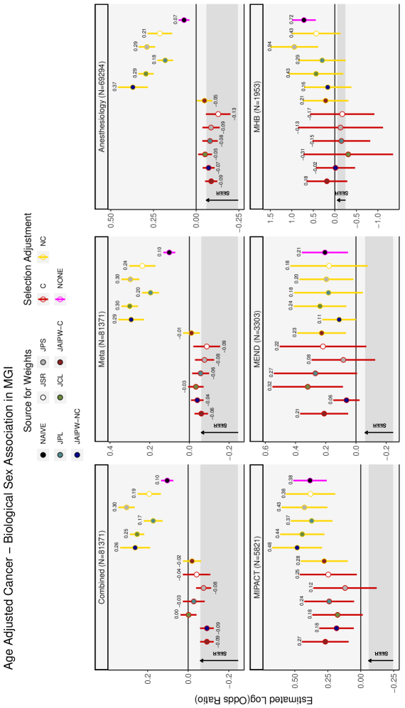
Figure S2: Estimates of the age-adjusted association between cancer and biological sex along with 95% C.I in using JAIPW, the four joint IPW methods and the unweighted logistic regression with and without including cancer as a selection variable. The grey band represents the true SEER estimates. The red bar corresponds to the unweighted logistic method. The yellow and pink bars correspond to the estimates of the JAIPW method and the four IPW methods without and with including cancer in the selection model respectively.

MGI-Anesthesiology: Subpart (C) of Figure S2 shows the performances of all the methods when implemented using data from MGI-Anesthesiology. Utilizing unweighted logistic regression, the age-adjusted estimate obtained was 0.07 with a 95% confidence interval (CI) of [0.04, 0.11], which is in the entirely opposite direction from the SEER registry reference range for marginal estimates, illustrated by the grey band in the accompanying figure. Upon incorporating cancer in the selection model, the estimates derived from the four IPW methods — PL, SR, PS, and CL are -0.08 (95% CI [-0.13, -0.04]), -0.13 (95% CI [-0.20, -0.06]), -0.08 (95% CI [-0.13, -0.04]), and -0.05 (95% CI [-0.09, -0.01]) respectively. These adjustments for selection bias position all of the 95% CIs from these IPW methods towards the direction of association indicated by SEER reference range. Conversely, when cancer is not included in the selection model, the estimates for all methods exhibit bias in the contrary direction underscoring the importance of considering cancer in the selection modeling. For the AIPW method, estimates yielded -0.09 (95% CI [-0.16, -0.09]), -0.07 (95% CI [-0.18, -0.11]) when the selection model included cancer and the auxiliary model did and did not include cancer, respectively. When the selection model excluded cancer with the auxiliary including it, the result was -0.05 (95% CI [-0.09, -0.01]).

MIPACT: Subpart (D) of Figure S2 shows the performances of all the methods when implemented using data from MIPACT. The estimated association between cancer and biological sex using the unweighted logistic regression method is considerably biased, with an estimate of 0.38 and a 95% confidence interval (CI) of [0.26, 0.51]. The IPW and AIPW methods were able to reduce the bias to some extent, particularly when cancer was included in the selection model or in the auxiliary score model (for AIPW).

MEND: Subpart (E) of Figure S2 shows the performance of all methods using data from MEND. The estimated age-adjusted association between cancer and biological sex from the unweighted logistic regression method exhibited bias, with an estimate of 0.21 and a 95% confidence interval (CI) of [0.05, 0.36]. The IPW and AIPW methods were able to reduce the bias to some extent, particularly when cancer was excluded from the selection model.

MHB: Subpart (F) of Figure S2 provides a comparative analysis of different methods when applied to the MHB data. The unweighted logistic regression method results in a highly biased estimate of the age-adjusted association between cancer and biological sex, with an estimated effect size of 0.72 and a 95% confidence interval of [0.44, 0.99]. This large bias may stem in part from the unique aspect of the MHB cohort, wherein biological sex is a variable that influences selection. IPW methods and JAIPW, when accounting for cancer, demonstrate some capacity to diminish the observed bias. Nonetheless, the estimates across all these methods are characterized by high variance. This is likely due to the modest sample size of the MHB cohort, which can lead to wider confidence intervals and less precise estimates.

Combined Data: Subpart (A) of Figure S2 shows the performances of all the methods when the cohorts are combined together. Using unweighted logistic regression, the estimate for the age adjusted association between cancer and biological sex was 0.10 [0.07, 0.13], which is in the entirely opposite direction from the SEER registry reference range for marginal estimates. Upon incorporating cancer in the selection model, the estimates derived from the four IPW methods—JPL, JSR, JPS, and JCL—are -0.03 (95% CI [-0.08, 0.03]), -0.04 (95% CI [-0.11, 0.02]), -0.08 (95% CI [-0.11, -0.04]), and 0.00 (95% CI [-0.04, 0.04]) respectively.For the JAIPW analysis, including cancer in either the selection model or the auxiliary model resulted in estimates of -0.09 (95% CI [-0.13, -0.06]), -0.09 (95% CI [-0.13, -0.06]), and -0.02 (95% CI [-0.06, 0.02]). All these methods corrected the direction of the cancer-biological sex association estimate.

Meta Combined: Subpart (B) of Figure S2 shows the performance of all meta-analyzed methods using data from the entire MGI. The unweighted logistic regression estimate for the age-adjusted association between cancer and biological sex was 0.10 [0.07, 0.13], which is in the entirely opposite direction from the SEER registry reference range for marginal estimates. Upon incorporating cancer in the selection model, the estimates derived from the four IPW methods—JPL, JSR, JPS, and JCL—were -0.06 (95% CI [-0.10, -0.01]), -0.09 (95% CI [-0.16, -0.02]), -0.08 (95% CI [-0.13, -0.03]), and -0.03 (95% CI [-0.07, 0.01]), respectively. For the JAIPW analysis, including cancer in either the selection model or the auxiliary model resulted in estimates of -0.06 (95% CI [-0.09, -0.03]), -0.04 (95% CI [-0.07, -0.01]), and -0.01 (95% CI [-0.05, 0.03]). All these methods corrected the direction of the cancer-biological sex association estimate.

Method Selection Model 1 Selection Model 2 Selection Model 3 Score Model Bias (times 100) ($\theta_{1}$) Bias (times 100) ($\theta_{2}$) Bias (times 100) ($\theta_{3}$) RMSE ($\theta_{1}$) RMSE ($\theta_{2}$) RMSE ($\theta_{3}$) Unweighted - - - - -5.28 (15.09%) -19.53 (43.40%) -5.74 (22.96%) 1 1 1 Meta SR Correct Correct Correct - 1.08 (3.10%) 1.64 (3.64%) 2.17 (8.66%) 0.22 0.03 0.38 Correct Correct Incorrect - 0.80 (2.28%) -2.17 (4.82%) 1.94 (7.77%) 0.19 0.04 0.32 Incorrect Incorrect Correct - 5.61 (16.03%) 4.71 (10.45%) 8.25 (33.00%) 1.13 0.06 2.04 Incorrect Incorrect Incorrect - 8.62 (24.63%) 7.31 (16.23%) 13.60 (54.38%) 2.48 0.15 5.23 Meta PL Correct Correct Correct - 0.48 (1.36%) -1.19 (2.64%) 0.79 (3.16%) 1.81 0.30 1.74 Correct Correct Incorrect - -0.46 (1.32%) -10.52 (23.37%) -1.26 (5.03%0 1.15 0.52 1.05 Incorrect Incorrect Correct - 5.79 (16.53%) -1.18 (2.63%) 6.28 (25.07%) 1.31 0.02 1.36 Incorrect Incorrect Incorrect - 6.43 (18.38%) 0.49 (1.09%) 11.54 (46.17%) 1.53 0.02 3.87 Meta PS Actual - - - - 0.19 (0.53%) -2.88 (6.40%) 4.82 (19.29%) 0.13 0.03 0.74 MetaPS Approx - - - - 2.72 (0.42%) -1.68 (3.73%) 15.51 (62.04%) 0.35 0.02 6.76 Meta CL Incorrect Incorrect Incorrect - 8.25 (23.57%) 5.82 (12.94%) 12.76 (51.04%) 2.28 0.10 4.60

Table S1: Bias and RMSE Comparison between the meta unweighted and the four meta IPW methods under simulation setup 2. Unweighted : Unweighted Logistic Regression, SR : Simplex Regression, PL : Pseudolikelihood, PS : Post Stratification, CL : Calibration

Method Selection Model 1 Selection Model 2 Selection Model 3 Score Model Sd Bias ($\theta_{1}$) Sd Bias ($\theta_{2}$) Sd Bias ($\theta_{3}$) CP ($\theta_{1}$) CP ($\theta_{2}$) CP ($\theta_{3}$) JSR Correct Correct Correct - 15.13% 10.27% 9.22% 0.93 0.91 0.93 Incorrect Incorrect Incorrect - 0.75% 4.45% 4.54% 0.05 0.05 0.00 JPL Correct Correct Correct - 20.24% 13.64% 18.36% 0.96 0.93 0.96 Incorrect Incorrect Incorrect - 5.90% 0.67% 3.79% 0.02 0.04 0.00 PS Actual - - - - 9.87% 3.57% 4.09% 0.85 0.93 0.25 JCL Incorrect Incorrect Incorrect - 2.71% 6.36% 0.75% 0.13 0.01 0.00 JAIPW Correct Correct Correct Correct 4.86% 14.57% 2.43% 0.97 0.91 0.96 Correct Correct Correct Incorrect 25.08% 22.32% 3.03% 0.93 0.94 0.95 Incorrect Incorrect Incorrect Correct 19.46% 15.15% 1.51% 0.96 0.92 0.94 Incorrect Incorrect Incorrect Incorrect 47.27% 34.14% 36.18% 0.02 0.20 0.02

Table S2: Relative standard error bias and coverage probability comparison between the four joint IPW methods and JAIPW under simulation setup 2. JSR : Joint Simplex Regression, JPL : Joint Pseudolikelihood, JPS : Joint Post Stratification, JCL : Joint Calibration and JAIPW : Joint Augmented Inverse Probability Weighted

Method Selection Model 1 Selection Model 2 Selection Model 3 Score Model Bias (times 100) ($\theta_{1}$) Bias (times 100) ($\theta_{2}$) Bias (times 100) ($\theta_{3}$) RMSE ($\theta_{1}$) RMSE ($\theta_{2}$) RMSE ($\theta_{3}$) Unweighted - - - - -8.47 (24.21%) -18.54 (41.20%) -13.43 (53.71%) 1 1 1 Unweighted Diff - - - - -10.03 (28.66%) -33.56 (74.57%) -3.91 (15.65%) 1.41 3.18 0.13 JSR Correct Correct Correct - -0.31 (0.88%) -0.66 (1.47%) -1.11 (4.47%) 0.04 0.01 0.02 Correct Correct Incorrect - 0.04 (0.11%) -1.72 (3.83%) -0.68 (2.76%) 0.04 0.02 0.02 Correct Incorrect Incorrect - -1.34 (3.84%) -7.39 (16.43%) -1.71 (6.86%) 0.06 0.17 0.03 Incorrect Incorrect Incorrect - -7.15 (20.42%) -16.30 (36.22%) -12.36 (49.43%) 0.71 0.78 0.86 JPL Correct Correct Correct - 0.29 (0.85%) -0.14 (0.32%) 0.10 (0.42%) 0.04 0.01 0.02 Correct Correct Incorrect - 0.62 (1.77%) -1.15 (2.55%) 0.51 (2.04%) 0.04 0.01 0.02 Correct Incorrect Incorrect - -0.84 (2.39%) -6.86 (15.23%) -0.39 (1.54%) 0.05 0.15 0.02 Incorrect Incorrect Incorrect - -7.29 (20.82%) -16.61 (36.92%) -12.15 (48.6%) 0.77 0.81 0.83 JPS Actual - - - - -2.60 (7.42%) -1.94 (4.32%) -1.36 (5.45%) 0.12 0.02 0.02 JPS Approx - - - - -4.11 (11.75%) -9.03 (20.10%) 4.87 (19.50%) 0.24 0.25 0.14 JCL Correct Correct Correct - -0.11 (0.30%) 0.34 (0.76%) -0.23 (0.91%) 0.04 0.01 0.02 JAIPW Correct Correct Correct Correct -0.69 (1.94%) -2.86 (6.36%)) -2.04 (8.15%) 0.16 0.15 0.15 Correct Correct Correct Incorrect -0.43 (1.23%) -1.83 (4.07%) -1.06 (4.23%) 0.06 0.03 0.04 Correct Correct Incorrect Correct -1.44 (4.11%) -3.08 (6.83%) -2.41 (9.62%) 0.39 0.20 0.20 Correct Correct Incorrect Incorrect -0.52 (1.50%) -3.93 (8.73%) -1.30 (5.19%) 0.22 0.12 0.08 Correct Incorrect Incorrect Correct -1.45 (4.14%) -2.39 (5.31%) -2.60 (10.40%) 0.23 0.15 0.16 Correct Incorrect Incorrect Incorrect -2.06 (5.87%) -7.98 (17.73%) -1.99 (7.98%) 0.11 0.20 0.05 Incorrect Incorrect Incorrect Correct -1.72 (4.91%) -3.59 (7.97%) -3.12 (12.46%) 0.51 0.34 0.48 Incorrect Incorrect Incorrect Incorrect -8.00 (22.86%) -16.89 (37.54%) -12.11 (48.44%) 0.92 0.84 0.83

Table S3: Bias and RMSE Comparison between the unweighted, four joint IPW methods and JAIPW under simulation setup 1. Unweighted : Unweighted Logistic Regression, JSR : Joint Simplex Regression, JPL : Joint Pseudolikelihood, JPS : Joint Post Stratification, JCL : Joint Calibration and JAIPW : Joint Augmented Inverse Probability Weighted

Method Selection Model 1 Selection Model 2 Selection Model 3 Score Model Bias (times 100) ($\theta_{1}$) Bias (times 100) ($\theta_{2}$) Bias (times 100) ($\theta_{3}$) RMSE ($\theta_{1}$) RMSE ($\theta_{2}$) RMSE ($\theta_{3}$) Unweighted - - - -8.39 (23.97%) -18.73 (41.64%) -11.59 (46.35%) 1 1 1 Meta SR Correct Correct Correct - -0.36 (1.03%) 0.32 (0.70%) -1.02 (4.06%) 0.05 0.01 0.04 Correct Correct Incorrect - -0.25 (0.73%) 0.13 (0.29%) -0.85 (3.39%) 0.05 0.01 0.04 Incorrect Incorrect Correct - -2.41 (6.89%) -2.20 (4.88%) -5.61 (22.46%) 0.13 0.02 0.27 Incorrect Incorrect Incorrect - -6.25 (17.85%) -15.73 (34.97%) -5.44 (21.76%) 0.55 0.74 0.20 Meta PL Correct Correct Correct - 0.18 (0.51%) 0.45 (0.99%) 0.23 (0.91%) 0.08 0.01 0.04 Correct Correct Incorrect - 0.35 (1.01%) 0.25 (0.55%) 0.43 (1.73%) 0.08 0.01 0.04 Incorrect Incorrect Correct - -4.45 (12.73%) -2.85 (6.33%) -6.26 (25.04%) 0.37 0.03 0.34 Incorrect Incorrect Incorrect - -6.41 (18.30%) -14.69 (32.64%) -5.05 (20.21%) 0.63 0.63 0.24 Meta PS Actual - - - - -3.53 (10.08%) -5.06 (11.24%) 4.35 (17.40%) 0.21 0.08 0.16 Meta PS Approx - - - - -4.09 (11.71%) -2.36 (5.24%) 3.83 (15.35%) 0.27 0.03 0.13 Meta CL Correct Correct Correct - 0.50 (1.44%) 0.06 (0.13%) -0.22 (0.86%) 0.05 0.01 0.02

Table S4: Bias and RMSE Comparison between the meta unweighted and the four meta IPW methods under simulation setup 1. Unweighted : Unweighted Logistic Regression, SR : Simplex Regression, PL : Pseudolikelihood, PS : Post Stratification, CL : Calibration

Method Selection Model 1 Selection Model 2 Selection Model 3 Score Model Sd Bias ($\theta_{1}$) Sd Bias ($\theta_{2}$) Sd Bias ($\theta_{3}$) CP ($\theta_{1}$) CP ($\theta_{2}$) CP ($\theta_{3}$) JSR Correct Correct Correct - 3.03% 9.67% 1.45% 0.95 0.92 0.91 Incorrect Incorrect Incorrect - 0.27% 11.93% 3.33% 0.08 0.00 0.00 JPL Correct Correct Correct - 3.49% 8.86% 1.13% 0.95 0.96 0.94 Incorrect Incorrect Incorrect - 0.29% 12.82% 4.64% 0.07 0.00 0.00 PS Actual - - - - 4.74% 4.58% 3.66% 0.71 0.78 0.84 JCL Correct Correct Correct - 2.23% 9.21% 0.43% 0.98 0.93 0.98 JAIPW Correct Correct Correct Correct 18.12% 15.00% 12.75% 0.93 0.90 0.91 Correct Correct Correct Incorrect 12.71% 9.32% 10.4% 0.90 0.84 0.85 Incorrect Incorrect Incorrect Correct 15.65% 8.85% 10.98% 0.92 0.90 0.93 Incorrect Incorrect Incorrect Incorrect 41.73% 42.16% 23.72% 0.00 0.00 0.00

Table S5: Relative standard error bias and coverage probability comparison between the four joint IPW methods and JAIPW under simulation setup 1. JSR : Joint Simplex Regression, JPL : Joint Pseudolikelihood, JPS : Joint Post Stratification, JCL : Joint Calibration and JAIPW : Joint Augmented Inverse Probability Weighted

Figure S3: Estimates of the age-adjusted log odds ratio of cancer with one unit change in Interquartile Range (IQR) of Polygenic Risk Score (PRS) for overall cancer along with 95% C.I in using JAIPW, the four JIPW methods and the unweighted logistic regression with and without including cancer as a selection variable. The black and violet bars correspond to the estimates of the JAIPW method and the four JIPW methods without and with including cancer in the selection model respectively.

References

- Barndorff-Nielsen and Jørgensen (1991) O. E. Barndorff-Nielsen and B. Jørgensen. Some parametric models on the simplex. Journal of multivariate analysis, 39(1):106–116, 1991.
- Beesley and Mukherjee (2022) L. J. Beesley and B. Mukherjee. Statistical inference for association studies using electronic health records: handling both selection bias and outcome misclassification. Biometrics, 78(1):214–226, 2022.
- Beesley et al. (2020) L. J. Beesley, L. G. Fritsche, and B. Mukherjee. An analytic framework for exploring sampling and observation process biases in genome and phenome-wide association studies using electronic health records. Statistics in Medicine, 39(14):1965–1979, 2020.
- Borenstein et al. (2010) M. Borenstein, L. V. Hedges, J. P. Higgins, and H. R. Rothstein. A basic introduction to fixed-effect and random-effects models for meta-analysis. Research synthesis methods, 1(2):97–111, 2010.
- Bradley et al. (2021) V. C. Bradley, S. Kuriwaki, M. Isakov, D. Sejdinovic, X.-L. Meng, and S. Flaxman. Unrepresentative big surveys significantly overestimated US vaccine uptake. Nature, 600(7890):695–700, 2021.
- Chen et al. (2020) Y. Chen, P. Li, and C. Wu. Doubly robust inference with nonprobability survey samples. Journal of the American Statistical Association, 115(532):2011–2021, 2020.
- Du et al. (2024) J. Du, X. Shi, D. Zeng, and B. Mukherjee. Doubly robust causal inference through penalized bias-reduced estimation: combining non-probability samples with designed surveys. arXiv preprint arXiv:2403.18039, 2024.
- Fritsche et al. (2020) L. G. Fritsche, S. Patil, L. J. Beesley, P. VandeHaar, M. Salvatore, Y. Ma, R. B. Peng, D. Taliun, X. Zhou, and B. Mukherjee. Cancer prsweb: an online repository with polygenic risk scores for major cancer traits and their evaluation in two independent biobanks. The American Journal of Human Genetics, 107(5):815–836, 2020.
- Holt and Smith (1979) D. Holt and T. F. Smith. Post stratification. Journal of the Royal Statistical Society: Series A (General), 142(1):33–46, 1979.
- Kundu et al. (2023) R. Kundu, X. Shi, J. Morrison, and B. Mukherjee. A framework for understanding selection bias in real-world healthcare data. arXiv preprint arXiv:2304.04652, 2023.
- Kundu et al. (2024) R. Kundu, X. Shi, J. Morrison, J. Barrett, and B. Mukherjee. A framework for understanding selection bias in real-world healthcare data. Journal of the Royal Statistical Society Series A: Statistics in Society, page qnae039, 2024.
- Luo and Song (2020) L. Luo and P. X.-K. Song. Renewable estimation and incremental inference in generalized linear models with streaming data sets. Journal of the Royal Statistical Society Series B: Statistical Methodology, 82(1):69–97, 2020.
- Rice et al. (2018) K. Rice, J. P. Higgins, and T. Lumley. A re-evaluation of fixed effect (s) meta-analysis. Journal of the Royal Statistical Society: Series A (Statistics in Society), 181(1):205–227, 2018.
- Robins et al. (1994) J. M. Robins, A. Rotnitzky, and L. P. Zhao. Estimation of regression coefficients when some regressors are not always observed. Journal of the American statistical Association, 89(427):846–866, 1994.
- Salvatore et al. (2024) M. Salvatore, R. Kundu, X. Shi, C. R. Friese, S. Lee, L. G. Fritsche, A. M. Mondul, D. Hanauer, C. L. Pearce, and B. Mukherjee. To weight or not to weight? the effect of selection bias in 3 large electronic health record-linked biobanks and recommendations for practice. Journal of the American Medical Informatics Association, page ocae098, 2024.
- Schoeler et al. (2023) T. Schoeler, D. Speed, E. Porcu, N. Pirastu, J.-B. Pingault, and Z. Kutalik. Participation bias in the uk biobank distorts genetic associations and downstream analyses. Nature Human Behaviour, 7(7):1216–1227, 2023.
- Tsiatis (2006) A. A. Tsiatis. Semiparametric theory and missing data. 2006.
- Wang and Kim (2021) H. Wang and J. K. Kim. Information projection approach to propensity score estimation for handling selection bias under missing at random. arXiv e-prints, pages arXiv–2104, 2021.
- West et al. (2021) B. T. West, R. J. Little, R. R. Andridge, P. S. Boonstra, E. B. Ware, A. Pandit, and F. Alvarado-Leiton. Assessing selection bias in regression coefficients estimated from nonprobability samples with applications to genetics and demographic surveys. The annals of applied statistics, 15(3):1556–1581, 2021.
- Williamson et al. (2012) E. J. Williamson, A. Forbes, and R. Wolfe. Doubly robust estimators of causal exposure effects with missing data in the outcome, exposure or a confounder. Statistics in medicine, 31(30):4382–4400, 2012.
- Wu (2003) C. Wu. Optimal calibration estimators in survey sampling. Biometrika, 90(4):937–951, 2003.
- Wu (2022) C. Wu. Statistical inference with non-probability survey samples. Survey Methodology, 48(2):283–311, 2022.
- Zawistowski et al. (2021) M. Zawistowski, L. G. Fritsche, A. Pandit, B. Vanderwerff, S. Patil, E. M. Scmidt, P. VanderHaar, C. M. Brummett, S. Keterpal, X. Zhou, et al. The michigan genomics initiative: a biobank linking genotypes and electronic clinical records in Michigan Medicine patients. medRxiv, 2021.