Analysis of $b\to c\ell\nu$ baryonic decay modes in SMEFT approach

Abstract

The flavor-changing neutral current decays of heavy bottom quark, alongside the flavor-changing charged current processes mediated by $b\to(c,u)$ in semileptonic $B$ decays are emerged as powerful tools for exploring physics beyond the Standard Model. In this work, we focus on the feasibility of interpreting the processes mediated by $b\to c\tau\nu$ transitions, in particular, the semileptonic $b$-baryonic decay modes $\Sigma_{b}\to\Sigma_{c}^{(*)}\tau^{-}\bar{\nu}_{\tau}$ and $\Xi_{b}\to\Xi_{c}\tau^{-}\bar{\nu}_{\tau}$ in the context of SMEFT approach. We perform a detailed analysis of the sensitivity of new physics operators on various observables such as branching ratio, forward-backward asymmetry parameter, lepton non-universal observable and the longitudinal polarization fraction of the $b$-baryonic decay channels.

I Introduction

In recent years, $b$-hadron decays have garnered significant attention as a promising avenue for exploring physics beyond the Standard Model (BSM). Both neutral and charged current $b$-decays offer a clean and controlled environment to investigate the sensitivity of new physics. Notably, the violation of Lepton Flavor Universality (LFU) - the principle that leptons couple to gauge bosons in a flavor-independent manner, has been observed in several observables in the semileptonic $B$ decays. The observables associated with the flavor changing charge current (FCCC) processes such as $R_{D^{(*)}}$, defined as

$$R_{D^{(*)}}=\frac{\mathcal{B}(B\to D^{(*)}\tau\nu)}{\mathcal{B}(B\to D^{(*)}\ell\nu)},$$ (1)

with ($\ell=\mu,e$), are potentially sensitive to the lepton flavor universality violation, making them ideal tools for testing new physics effects. Several measurements on $R_{D^{(*)}}$ at BaBar BaBar:2012obs ; BaBar:2013mob , Belle Belle:2015qfa ; Belle:2016ure ; Abdesselam:2016xqt ; Belle:2019rba , and LHCb LHCb:2015gmp ; LHCb:2017smo collaborations along with HFLAV Group HFLAV:2022esi show deviation of approximately $3.3\sigma$ from the Standard Model (SM) prediction Fajfer:2012vx ; Kamenik:2008tj ; Aoki:2016frl . Other observables, such as $P_{\tau}(D)$ and $F_{L}(D)$, which involve the ratio of $B$ meson decays for polarized and unpolarized final states, exhibit deviations from SM predictions at the $(1.5-2)\sigma$ level Belle:2016dyj ; Asadi:2018sym ; Alok:2016qyh . Numerous global analyses have explored the tension in $R_{D^{(*)}}$ by incorporating new physics (NP) contributions. Specifically, various one and two dimensional NP scenarios have been proposed as plausible solutions, with particular emphasis on new physics affecting only the $\tau$ channel Ray:2023xjn . Similarly, the ratio of the branching fractions $R_{J/\psi}=\mathcal{B}(B\to J/\psi\tau\nu)/\mathcal{B}(B\to J/\psi\ell\nu)$ measured by LHCb collaboration LHCb:2017vlu also indicates about $2\sigma$ discrepancy above the SM value Dutta:2017xmj .

Motivated by the insights from the above decay processes, we investigate semileptonic $b$-baryon decays, specifically focusing on the exclusive $\Sigma_{b}\to\Sigma_{c}^{(*)}\tau^{-}\bar{\nu}_{\tau}$ and $\Xi_{b}\to\Xi_{c}\tau^{-}\bar{\nu}_{\tau}$ processes. These decay modes could offer valuable information for probing new physics effects in the context of $b\to c\ell\nu$ quark-level transitions. Investigation of these decays offers valuable insights into the weak interaction properties and underlying dynamics of heavy baryons, as well as their sensitivity to NP. Furthermore, semileptonic decays of heavy $b$-baryons provide a valuable complementary perspective to meson decay modes, enriching the search for new physics by exploring different aspects of particle interactions. On the experimental front, significant progress has been made in studying heavy baryons containing a $b$ quark with substantial data accumulation from experiments like the Tevatron and LHC. The $\Xi_{b}^{0,+,-}$ baryons have been observed by the CDF, D0 CDF:2007cgg ; D0:2007gjs , and LHCb LHCb:2014chk ; LHCb:2014wqn ; LHCb:2013jih ; LHCb:2014jst ; LHCb:2015une ; LHCb:2016hha ; LHCb:2017fwd collaborations. Additionally, the CDF and LHCb collaborations CDF:2011ac ; LHCb:2018haf have reported clear signals for the four strongly decaying baryon states: $\Xi_{b}^{+}$, $\Xi_{b}^{-}$, $\Xi_{b}^{*+}$, and $\Xi_{b}^{*-}$. While the $\Sigma_{b}$ baryon primarily decays through strong interactions, measuring its weak branching fraction can be challenging. Yet, investigating semileptonic decay modes may yield significant insights, as they exhibit a higher sensitivity to departures from SM predictions, potentially pointing to the new physics Ke:2019smy .

In this work, we adopt the SMEFT framework, assuming that the scale of NP exceeds the electroweak scale and that no additional light particles exist below this scale. Given the lack of direct evidence for new particles, a model-independent effective field theory approach is ideal. Within this framework, the low energy effective field theory (LEFT) can describe the $b\to c\ell\nu$ transition below the electroweak scale, respecting SM gauge symmetry $SU(3)_{C}\times SU(2)_{L}\times U(1)_{Y}$. We assume the new physics scale $\Lambda$ to be 1 TeV, which is much higher than the electroweak (EW) scale. In this context, the physics between the EW scale and $\Lambda$ can be effectively described by the Standard Model Effective Field Theory (SMEFT), which includes all SM particles. To connect low-energy observables with new physics, it is essential to match the operators in the LEFT to those in SMEFT and then run down to $m_{b}$ scale. The SMEFT operators that generate the $b\to c\ell\nu_{\ell}$ transition also produce LEFT operators relevant for the $b\to s\ell^{+}\ell^{-}$ and $b\to s\nu\nu$ processes. This connection means that the constraints from $b\to c\ell\nu$ processes are inherently tied to bounds from $b\to s\ell\ell$ and $b\to s\nu\nu$ processes. Therefore, the limits derived from $b\to s\ell^{+}\ell^{-}$ and $b\to s\nu\nu$ transitions serve as complementary constraints on the decay modes being investigated. Various theoretical analyses have been conducted to explore the baryonic $b$ quark decay processes in detail Ebert:2006rp ; Singleton:1990ye ; Ivanov:1996fj ; Ivanov:1998ya ; Ke:2012wa ; Wang:2017mqp ; Rajeev:2019ktp , providing valuable insights into their underlying dynamics. We mainly focus on the various decay observables such as branching ratio, forward-backward asymmetry, covexity parameter and lepton polarisation asymmetry of the exclusive $\Sigma_{b}\to\Sigma_{c}^{(*)}\tau^{-}\bar{\nu}_{\tau}$ and $\Xi_{b}\to\Xi_{c}\tau^{-}\bar{\nu}_{\tau}$ transitions. We also scrutinize nature of the lepton non universality of the above decay channels.

This paper is organized as follows. In section II, We will first introduce the LEFT to describe the $b\to c\tau\nu$ process and eventually match with the SMEFT operators. In section III, we discuss various observables associated with the exclusive $\Sigma_{b}\to\Sigma_{c}^{(*)}\tau^{-}\bar{\nu}_{\tau}$ and $\Xi_{b}\to\Xi_{c}\tau^{-}\bar{\nu}_{\tau}$ processes. Section IV focuses on the new physics analysis including the constraint on the NP couplings within both one-dimensional and two-dimensional scenarios. We then examine the effect of these newly fitted couplings on the $b\to c\tau\bar{\nu}$ baryonic decay observables in section V. Finally we conclude our analysis in section VI.

II Theoretical Framework

This section outlines the framework for the $b\to c\ell\nu$ process, along with other relevant transitions such as $b\to s\ell\ell$ and $b\to s\nu\nu$ within the LEFT. It also contains the details of the operators relevant to those in the SMEFT at $\mu(m_{b})$ scale. In this work, we discuss the effects of the NP couplings, assuming that all Wilson coefficients are real.

II.1 Low Energy Effective Field Theory

II.1.1 $b\to c\ell\nu$

The most general low-energy effective Hamiltonian relevant for $b\to c\ell\nu$ transition, considering only the left-handed neutrinos, is given as Sakaki:2013bfa

$$\begin{split}\mathcal{H}_{eff}=\mathcal{H}_{eff}^{SM}+\frac{4G_{F}}{\sqrt{2}}V_{cb}\sum_{i,l}C_{i}^{(l)}\mathcal{O}_{i}^{(l)}+h.c.\end{split}$$ (2)

Here $\mathcal{O}^{(\ell)}_{i}$ ($i=V_{L},V_{R},S_{L},S_{R},T$) are local effective operators, $C_{i}^{(\ell)}$ are Wilson coefficients encoding contributions of short distance new physics, $V_{cb}$ is the Cabbibo-Kobayasi-Maskawa (CKM) matrix element, $G_{F}$ is the fermi constant, and $\ell$ stands for the lepton flavor indices. The relevant set of local operators with mass dimension-6, are presented as

$$O_{V_{L}}^{(\ell)}=(\bar{u}_{L}\gamma^{\mu}b_{L})(\bar{\ell}_{L}\gamma_{\mu}\nu_{\ell L}),\hskip 28.45274ptO_{V_{R}}^{(\ell)}=(\bar{u}_{R}\gamma^{\mu}b_{R})(\bar{\ell}_{L}\gamma_{\mu}\nu_{\ell L}),$$

$$O_{S_{L}}^{(\ell)}=(\bar{u}_{R}b_{L})(\bar{\ell}_{R}\nu_{\ell L}),\hskip 48.36958ptO_{S_{R}}^{(\ell)}=(\bar{u}_{L}b_{R})(\bar{\ell}_{R}\nu_{\ell L}),$$

$$O_{T}^{(\ell)}=(\bar{u}_{R}\sigma^{\mu\nu}b_{L})(\bar{\ell}_{R}\sigma_{\mu\nu}\nu_{\ell L}),$$ (3)

where the $O_{V_{L,R}}^{(\ell)}$, $O_{S_{L,R}}^{(\ell)}$ and $O_{T}^{(\ell)}$ are respectively known are vector, scalar and tensor operators.

II.1.2 $b\to s\ell\ell$

The weak effective Hamiltonian describing the $b\to s\ell\ell$ decay is given as Bobeth:1999mk ; Bobeth:2001jm

$$\begin{split}\mathcal{H}_{eff}=-\frac{4G_{F}}{\sqrt{2}}V_{tb}V^{*}_{ts}\frac{\alpha_{em}}{4\pi}\sum_{i=9,10,S,P}\big{(}C_{i}\mathcal{O}_{i}+C_{i}\mathcal{O^{\prime}}_{i}\big{)},\end{split}$$ (4)

where $V_{tb}V_{ts}^{*}$ is the product of the CKM matrix elements. The relevant operators for this process are expressed as follows,

$$\begin{split}&\mathcal{O}^{(\prime)}_{9}=\big{[}\bar{s}\gamma^{\mu}P_{L(R)}b\big{]}\big{[}\ell\gamma_{\mu}\ell\big{]}\,,\quad\mathcal{O}^{(\prime)}_{10}=\big{[}\bar{s}\gamma^{\mu}P_{L(R)}b\big{]}\big{[}\ell\gamma_{\mu}\gamma_{5}\ell\big{]}\;,\\ &\mathcal{O}_{S}^{(\prime)}=\big{[}\bar{s}P_{R(L)}b\big{]}\big{[}\ell\ell\big{]}\,,\quad\quad\quad\mathcal{O}_{P}^{(\prime)}=\big{[}\bar{s}P_{R(L)}b\big{]}\big{[}\ell\gamma_{5}\ell\big{]}\,.\end{split}$$ (5)

Here, the operators $\mathcal{O}_{9(10),S(P)}$ represent the (axial)vector and (pseudo)scalar operators, respectively. The primed operators $\mathcal{O}_{i}^{\prime}$ can be obtained by flipping the chirality of the operators $\mathcal{O}_{i}$. The $C^{(\prime)}_{9,10,S,P}$ are the Wilson coefficients that have zero value in the SM and can have a non-zero value in various new physics scenarios.

II.1.3 $b\to s\nu\nu$

The generic effective Hamiltonian for $b\to s\nu\bar{\nu}$ is as follows Buras:2014fpa ; Altmannshofer:2009ma

$$\mathcal{L}_{\mathrm{eff}}^{b\to s\nu\bar{\nu}}=\frac{4G_{F}}{\sqrt{2}}V_{tb}V_{ts}^{\ast}\frac{\alpha}{4\pi}\sum_{\ell}\left(C^{\nu_{\ell}}_{L}\mathcal{O}^{\nu_{\ell}}_{L}+C^{\nu_{\ell}}_{R}\mathcal{O}^{\nu_{\ell}}_{R}\right)+\mathrm{h.c.}\,,$$ (6)

with

$$\mathcal{O}^{\nu_{\ell}}_{L}= (\bar{s}\gamma_{\mu}P_{L}b)(\bar{\nu}_{\ell}\gamma^{\mu}(1-\gamma_{5})\nu_{\ell})\,, \mathcal{O}^{\nu_{\ell}}_{R}= (\bar{s}\gamma_{\mu}P_{R}b)(\bar{\nu}_{\ell}\gamma^{\mu}(1-\gamma_{5})\nu_{\ell})\,.$$ (7)

In Eq. (6), $\alpha=e^{2}/4\pi$ is the fine structure constant, $V_{tb}$ and $V_{ts}$ are the relevant CKM matrix elements, and $P_{L,R}=(1\mp\gamma_{5})/2$ stand for the (left, right) handed projection operators. The operator $\mathcal{O}_{R}^{\nu_{\ell}}$ can only arise in the presence of NP, so $C^{\nu_{\ell}}_{R,\mathrm{SM}}=0$, while $\mathcal{O}_{L}^{\nu_{\ell}}$ can originate from either the SM or NP, with $C^{\nu_{\ell}}_{L,\mathrm{SM}}=-6.32(7)$.

II.2 Standard Model Effective Field Theory

In the SMEFT expansion to the dimension-six order, we study the correlations among various low-energy observables. We detail the relevant Lagrangian in the form of the SMEFT operators and then explore various observables that are correlated with $b\to c\ell\nu$ decays in this context. Above the EW scale, we use the following SMEFT effective Lagrangian at mass dimension-six to parameterize model-independent effects of high-scale NP,

$$\mathcal{L_{\mathrm{eff}}}=\mathcal{L_{\mathrm{SM}}}+\sum_{Q_{i}=Q_{i}^{\dagger}}\frac{C_{i}}{\Lambda^{2}}Q_{i}+\sum_{Q_{i}\neq Q_{i}^{\dagger}}\left(\frac{C_{i}}{\Lambda^{2}}Q_{i}+\frac{C_{i}^{\ast}}{\Lambda^{2}}Q_{i}^{\dagger}\right)\;,$$ (8)

with the cut-off scale $\Lambda$.

In the SMEFT, the operators which will be relevant for the $b\to c\ell^{-}\bar{\nu}_{\ell}$ transitions are given by Aebischer:2015fzz

$$Q^{(3)}_{\ell q} = (\bar{\ell}_{i}\gamma_{\mu}\tau^{I}\ell_{j})(\bar{q}_{k}\gamma^{\mu}\tau^{I}q_{l}),\leavevmode\nobreak\ \leavevmode\nobreak\ \leavevmode\nobreak\ \leavevmode\nobreak\ \leavevmode\nobreak\ \leavevmode\nobreak\ Q_{\phi ud}=i(\tilde{\phi}^{\dagger}D_{\mu}\phi)(\bar{u}_{i}\gamma^{\mu}d_{j}),$$

$$Q_{\ell edq} = (\bar{\ell}_{i}^{a}e_{j})(\bar{d}_{k}q_{l}^{a}),\leavevmode\nobreak\ \leavevmode\nobreak\ \leavevmode\nobreak\ \leavevmode\nobreak\ \leavevmode\nobreak\ \leavevmode\nobreak\ \leavevmode\nobreak\ \leavevmode\nobreak\ \leavevmode\nobreak\ \leavevmode\nobreak\ \leavevmode\nobreak\ \leavevmode\nobreak\ \leavevmode\nobreak\ \leavevmode\nobreak\ \leavevmode\nobreak\ \leavevmode\nobreak\ \leavevmode\nobreak\ Q^{(1)}_{\ell equ}=(\bar{\ell}_{i}^{a}e_{j})\epsilon_{ab}(\bar{q}_{k}^{b}u_{l}),$$

$$Q^{(3)}_{\ell equ} = (\bar{\ell}_{i}^{a}\sigma^{\mu\nu}e_{j})\epsilon_{ab}(\bar{q}_{k}^{b}\sigma_{\mu\nu}u_{l}),\leavevmode\nobreak\ \leavevmode\nobreak\ \leavevmode\nobreak\ \leavevmode\nobreak\ Q^{(3)}_{\phi q}=(\phi^{\dagger}i\overset{\leftrightarrow}{D}_{\mu}\phi)(\bar{q}_{i}\tau^{I}\gamma^{\mu}q_{j}).$$ (9)

In the above equation, $\ell,q$ and $\phi$ represent lepton, quark and Higgs $SU(2)_{L}$ doublets, while the right-handed isospin singlets are denoted by $e$, $u$ and $d$. Here we collect the dimension six operators contributing to the $b\to c\ell\nu$, $b\to s\ell\ell$ and $b\to s\nu\nu$ transitions. The operators $Q^{(3)}_{\ell q}$,$Q_{\ell edq}$,$Q^{(3)}_{\ell equ}$,$Q^{(1)}_{\ell equ}$ contribute to the $b\to c\ell\nu$ as contact interaction and $Q^{(3)}_{\phi q}$,modify the left and right-handed W couplings with quark.

Following the method discussed above, a tree-level matching of the SMEFT operators given in Eq. (II.2) to the effective operator basis defined in Eq.  (3) will result in the following WCs at the $m_{b}$ scale for $b\to c\ell^{-}\bar{\nu}_{\ell}$ decays Aebischer:2015fzz

$$C_{V_{L}} = -\frac{v^{2}}{\Lambda^{2}}\frac{V_{cs}}{V_{cb}}\tilde{C}^{(3)ll23}_{\ell q},\leavevmode\nobreak\ \leavevmode\nobreak\ \leavevmode\nobreak\ \leavevmode\nobreak\ \leavevmode\nobreak\ \leavevmode\nobreak\ \leavevmode\nobreak\ C_{V_{R}}=0,$$

$$\tilde{C}_{S_{L}} = -\frac{v^{2}}{2\Lambda^{2}}\frac{V_{cs}}{V_{cb}}\tilde{C}^{(1)*ll32}_{\ell equ},\leavevmode\nobreak\ \leavevmode\nobreak\ \leavevmode\nobreak\ \leavevmode\nobreak\ \leavevmode\nobreak\ \tilde{C}_{S_{R}}=-\frac{v^{2}}{2\Lambda^{2}}\frac{V_{tb}}{V_{cb}}\tilde{C}^{*ll32}_{\ell edq},$$

$$\tilde{C}_{T} = -\frac{v^{2}}{2\Lambda^{2}}\frac{V_{tb}}{V_{cb}}\tilde{C}^{*(3)ll32}_{\ell equ}.$$ (10)

III The decay Observables of $B_{b}\to B_{c}\ell\bar{\nu}$ processes

The differential decay distribution for $B_{b}\to B_{c}\ell\nu$ decays, where $B_{b}$ and $B_{c}$ represent the bottom and charmed baryons, can be expressed in terms of the helicity amplitudes $H^{V/A}_{\lambda_{2}\lambda_{W}}$, as described in Ref. Dutta:2013qaa . This formulation is represented through the parameters $\mathcal{A}_{1}$, $\mathcal{A}_{2}$, $\mathcal{A}_{3}$, and $\mathcal{A}_{4}$, and is given by:

$$\frac{d^{2}\Gamma}{dq^{2}\,d\cos\theta}=\mathcal{N}\left(1-\frac{m_{\ell}^{2}}{q^{2}}\right)^{2}\left[\mathcal{A}_{1}+\frac{m_{\ell}^{2}}{q^{2}}\mathcal{A}_{2}+2\mathcal{A}_{3}+\frac{4m_{\ell}}{\sqrt{q^{2}}}\mathcal{A}_{4}\right],$$ (11)

where $\theta$ denotes the angle between the momentum vector $\vec{P}_{B_{c}}$ and the lepton’s three-momentum in the $\ell-\nu$ rest frame. The normalization factor $\mathcal{N}$ is expressed as

$$\mathcal{N}=\frac{G_{F}^{2}\,|V_{cb}|^{2}\,q^{2}|\vec{P}_{B_{c}}|}{512\,\pi^{3}\,m_{B_{b}}^{2}}\left(1-\frac{m_{\ell}^{2}}{q^{2}}\right)^{2}.$$ (12)

The components $\mathcal{A}_{i}$ are defined as follows:

$$\mathcal{A}_{1} =2\sin^{2}\theta\left(H^{2}_{\frac{1}{2}0}+H^{2}_{-\frac{1}{2}0}\right)+\left(1-\cos\theta\right)^{2}H^{2}_{\frac{1}{2}1}+\left(1+\cos\theta\right)^{2}H^{2}_{-\frac{1}{2}-1},$$

$$\mathcal{A}_{2} =2\cos^{2}\theta\left(H^{2}_{\frac{1}{2}0}+H^{2}_{-\frac{1}{2}0}\right)+\sin^{2}\theta\left(H^{2}_{\frac{1}{2}1}+H^{2}_{-\frac{1}{2}-1}\right)+2\left(H^{2}_{\frac{1}{2}t}+H^{2}_{-\frac{1}{2}t}\right)$$

$$\quad-4\cos\theta\left(H_{\frac{1}{2}t}H_{\frac{1}{2}0}+H_{-\frac{1}{2}t}H_{-\frac{1}{2}0}\right),$$

$$\mathcal{A}_{3} =\left(H^{SP}_{\frac{1}{2}0}\right)^{2}+\left(H^{SP}_{-\frac{1}{2}0}\right)^{2},$$

$$\mathcal{A}_{4} =-\cos\theta\left(H_{\frac{1}{2}0}H^{SP}_{\frac{1}{2}0}+H_{-\frac{1}{2}0}H^{SP}_{-\frac{1}{2}0}\right)+\left(H_{\frac{1}{2}t}H^{SP}_{\frac{1}{2}0}+H_{-\frac{1}{2}t}H^{SP}_{-\frac{1}{2}0}\right).$$ (13)

The helicity amplitudes $H^{V/A}_{\lambda_{2}\lambda_{W}}$ and $H^{SP}_{\lambda_{2}\lambda_{W}}$ are essential for defining these terms, and their details are provided in Refs. Rajeev:2019ktp ; Dutta:2013qaa . This framework serves as the basis for analyzing the decay observables associated with the process. Now, we define several $q^{2}$-dependent observables to characterize the decay processes. These include the total differential branching ratio $dBr/dq^{2}$, the ratio of branching fractions $R^{(*)}_{B_{c}}(q^{2})$, the forward-backward asymmetry $A_{FB}^{l}(q^{2})$ and the polarization fraction of the charged lepton $P^{l}(q^{2})$. Another key observable is the convexity parameter $C_{F}^{l}(q^{2})$, determined by integrating the $\cos^{2}\theta$ dependence of the angular distribution. These observables are defined for decay modes $B_{b}\to B_{c}^{(*)}\ell\bar{\nu}$ as follows:

• The differential branching ratio

$$dBr/dq^{2}=\tau_{B_{b}}d\Gamma/dq^{2}$$ (14)

• Lepton non-uiversal observable

$$R_{B_{c}^{(*)}}(q^{2})=\frac{\frac{d\Gamma}{dq^{2}}(B_{b}\to B_{c}^{(*)}\tau^{-}\bar{\nu}_{\tau})}{\frac{d\Gamma}{dq^{2}}(B_{b}\to B_{c}^{(*)}\ell^{-}\bar{\nu}_{\ell})}$$ (15)

• Forward-backward asymmetry

$$A_{FB}^{\tau}(q^{2})=\frac{\large(\int_{0}^{1}-\int_{1}^{0}\large)\frac{d^{2}\Gamma}{dq^{2}d\cos\theta}d\cos\theta}{\large(\int_{0}^{1}+\int_{1}^{0}\large)\frac{d^{2}\Gamma}{dq^{2}d\cos\theta}d\cos\theta}$$ (16)

• Convexity parameter

$$C_{F}^{\tau}(q^{2})=\frac{1}{d\Gamma/dq^{2}}\frac{d^{2}}{d\cos\theta}\left(\frac{d^{2}\Gamma}{dq^{2}d\cos\theta}\right)$$ (17)

.

• Longitudinal polarisation fraction

$$P_{L}^{\tau}(q^{2})=\frac{{d\Gamma^{\lambda_{\tau}=1/2}}/{dq^{2}}-{d\Gamma^{\lambda_{\tau}=-1/2}}/{dq^{2}}}{{d\Gamma^{\lambda_{\tau}=1/2}}/{dq^{2}}+{d\Gamma^{\lambda_{\tau}=-1/2}}/{dq^{2}}},$$ (18)

where $d\Gamma^{\lambda_{\tau}=\pm 1/2}/dq^{2}$ are the helicity dependent differential decay rates.

IV New Physics Analysis in SMEFT

IV.1 Constraints on the SMEFT coefficient(s)

This subsection focuses on evaluating the SMEFT Wilson coefficients, such as $C_{\ell q}^{(3)}$, $C_{\ell equ}^{(1)}$, and $C_{\ell edq}$, by analyzing various $B$ mesonic observables mediated by the $b\to c\tau\nu_{\tau}$ transitions. We also examine observables associated with $b\to s\tau^{+}\tau^{-}$ and $b\to s\nu\nu$ transitions to impose complementary constraints on the SMEFT Wilson coefficients. However, among the couplings, only $C_{\ell q}^{(3)}$ contributes to $b\to c\tau\nu$, $b\to s\tau^{+}\tau^{-}$ and $b\to s\nu\bar{\nu}$ mediated decays.

We employ the experimental observations given in Table 1 to constrain the NP parameters. The allowed parameter scan of the NP couplings in 1$\sigma$, 2$\sigma$ and 3$\sigma$ regions are presented in Fig. 1 where a naive chi-square analysis to obtain the best fit values.

Observables	Experimental Value
$R_{D}$	$0.357\pm 0.029\pm 0.014$ HFLAV:2022link
$R_{D^{*}}$	$0.284\pm 0.010\pm 0.012$  HFLAV:2022link
$P_{\tau}(D^{*})$	$-0.38\pm 0.51^{+0.21}_{-0.16}$ Belle:2019ewo
$F_{L}(D^{*})$	$0.60\pm 0.08\pm 0.04$ Belle:2019ewo
$R(\Lambda_{c})$	$0.242\pm 0.026\pm\pm 0.040$ LHCb:2022piu
$\mathcal{B}(B\to K^{+}\nu\bar{\nu})$	$(2.4\pm 0.7)\times 10^{-5}$ Belle-II:2023esi
$\mathcal{B}(B^{0}\to K^{*0}\nu\bar{\nu})$	$<1.8\times 10^{-5}$ Belle:2017oht
$\mathcal{B}(B_{s}\to\tau^{+}\tau^{-})$	$<6.8\times 10^{-3}$ LHCb:2017myy
$\mathcal{B}(\bar{B}\to K^{+}\tau^{+}\tau^{-})$	$<2.25\times 10^{-3}$ BaBar:2016wgb

Table 1: Experimental values of various $b\to c\tau\nu_{\tau}$, $b\to s\nu\bar{\nu}$, and $b\to s\tau^{+}\tau^{-}$ observables.

The relevant formula for the chi-square analysis is defined as

$$\chi^{2}(C^{\rm NP})=\sum_{i}\frac{\Big{(}{\cal O}_{i}^{\rm Th}(C^{\rm NP})-{\cal O}_{i}^{\rm Exp}\Big{)}^{2}}{(\Delta{\cal O}_{i}^{\rm Exp})^{2}+(\Delta{\cal O}_{i}^{\rm SM})^{2}},$$ (19)

where ${\cal O}_{I}^{\rm Th}$ and ${\cal O}_{I}^{\rm Exp}$ represent the theoretical values and the measured central value of the observables, respectively. The denominator represents the error associated with the SM and experimental values. From this analysis, the best-fit values of the SMEFT couplings in 1D and 2D scenarios are provided in Table 2.

SMEFT couplings	$b\to c\tau\nu_{\tau}$	$b\to s\tau^{+}\tau^{-}$	$b\to s\nu\bar{\nu}$
$C_{lq}^{(3)}$	1.397	-0.456	-0.0748
$C_{lequ}^{(1)}$	$-0.054$	—	—
$C_{ledq}$	$-0.087$	—	—
$(C_{lq}^{(3)},C_{lequ}^{(1)})$	(-0.013, -0.042)	—	—
$(C_{lq}^{(3)},C_{ledq})$	(-0.007, -0.058)	—	—
$(C_{lequ}^{(1)},C_{ledq})$	(1.290, 0.675)	—	—

Table 2: Best-fit values of NP couplings in 1D and 2D scenario(s).

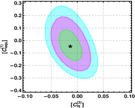
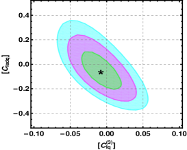
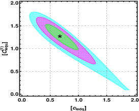
Figure 1: Allowed parameter scan in 1$\sigma$ (green), 2$\sigma$ (magenta), and 3$\sigma$ (cyan) regions. The black star denotes the best-fit value.

V Results and Discussions

After determining the SMEFT couplings using the measured observables given in Table 1, we analyze the $q^{2}$-dependence of several observables associated with the baryonic decay modes $\Sigma_{b}\to\Sigma_{c}^{(*)}\tau^{-}\bar{\nu}_{\tau}$ and $\Xi_{b}\to\Xi_{c}\tau^{-}\bar{\nu}_{\tau}$. The impact of the three one-dimensional scenarios is found to be less significant; hence, our focus shifts to the two-dimensional scenarios. The details of our analysis are outlined below.

V.1 Analysis of $\Xi_{b}\to\Xi_{c}\tau^{-}\bar{\nu}_{\tau}$Process

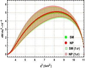
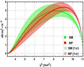
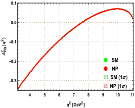
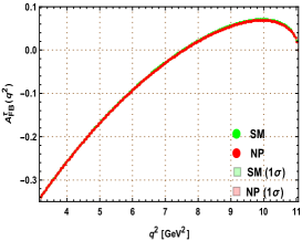
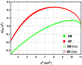
Figure 2: $d\text{Br}/dq^{2}$ and $A_{FB}$ for $\Xi_{b}\to\Xi_{c}\tau^{-}\bar{\nu}_{\tau}$ in $(C_{lq}^{(3)},C_{lequ}^{(1)})$ (left), $(C_{lq}^{(3)},C_{ledq})$ (middle), and $(C_{lequ}^{(1)},C_{ledq})$ (right). Top panel: branching ratio, Bottom panel: forward-backward asymmetry.

Fig. 2 (top panel) illustrates the variation of the differential branching ratio as a function of di-lepton mass squared ($q^{2}$) distribution. The green band represents the SM contribution, while the red band corresponds to predictions under the new physics framework. Among the three two-dimensional scenarios, the combination of Wilson coefficients $(C_{lequ}^{(1)},C_{ledq})$ exhibits a significant deviation from the SM, emphasizing the potential impact of the associated operators on the observed behavior.

Similarly, Fig. 2 (bottom panel) shows the forward-backward asymmetry, revealing a pronounced shift in the zero-crossing point from approximately $4.2\leavevmode\nobreak\ \mathrm{GeV}^{2}$ to $7.5\leavevmode\nobreak\ \mathrm{GeV}^{2}$. This behavior strongly suggests the influence of new physics contributions associated with the Wilson coefficients $(C_{lequ}^{(1)},C_{ledq})$. In contrast, the other scenarios remain largely consistent with the SM predictions.

On the other hand, we observe a notable convexity pattern in the low $q^{2}$ region, characterized by negligible uncertainty, arising from the simultaneous impact of the new physics contributions of the $C_{lequ}^{(1)}$ and $C_{ledq}$ couplings. This is shown in Fig. 3.

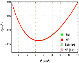
Figure 3: The $q^{2}$ distribution of convexity parameter of $\Xi_{b}\to\Xi_{c}\tau^{-}\bar{\nu}_{\tau}$ process. The description of couplings is same as Fig. 2

Fig. 4 depicts the deviation in the lepton polarisation asymmetry observable indicates prominent deviation for all $q^{2}$ range in the presence of the couplings $(C_{lequ}^{(1)},C_{ledq})$. However, we observe a mild deviation the presence of $(C_{lq}^{(3)},C_{ledq})$ in the high $q^{2}$ region.

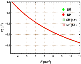
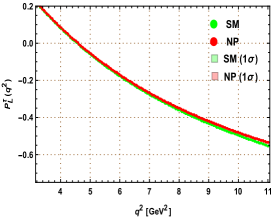
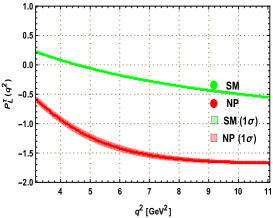
Figure 4: The $q^{2}$ dependence of the longitudinal polarization fraction $\Xi_{b}\to\Xi_{c}\tau^{-}\bar{\nu}_{\tau}$ process. The description of couplings is same as Fig. 2.

We also analyze the $q^{2}$-dependence of the lepton non-universality observable, as illustrated in Fig. 5. A significant deviation from the SM prediction is observed at large $q^{2}$ values, particularly evident in the right panel. In contrast, the low $q^{2}$ region shows only a mild discrepancy from the SM. Notably, such discrepancies are absent in the other two scenarios, where the predictions align closely with the SM across the entire $q^{2}$ range. This indicates that the observed deviations are strongly dependent on the specific scenario considered.

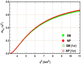
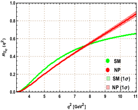
Figure 5: The $q^{2}$ behavior of $R_{\Sigma_{b}}$ in the $\Xi_{b}\to\Xi_{c}\tau^{-}\bar{\nu}_{\tau}$ process. The description of couplings is same as Fig. 2.

V.2 Analysis of $\Sigma_{b}\to\Sigma_{c}\tau^{-}\bar{\nu}_{\tau}$ Process

This subsection will explore the various observables of the $\Sigma_{b}\to\Sigma_{c}\tau^{-}\bar{\nu}_{\tau}$ channel. The behavior of the $q^{2}$ distribution are discussed below.

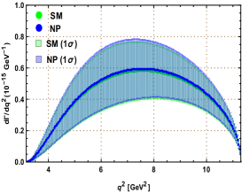
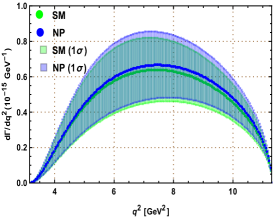
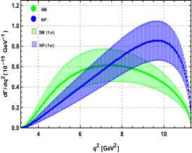
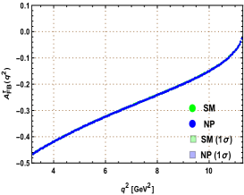
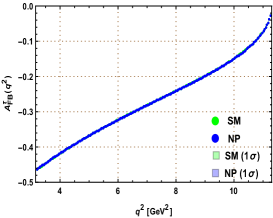
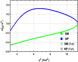
Figure 6: $d\text{Br}/dq^{2}$ and $A_{FB}$ for $\Sigma_{b}\to\Sigma_{c}\tau^{-}\bar{\nu}_{\tau}$ processes. The description of couplings is same as Fig. 2. Top panel: branching ratio, Bottom panel: forward-backward asymmetry.

Figure 6 (top panel) depicts the variation of the differential branching ratio as a function of $q^{2}$. The green band represents the prediction based on the SM contribution. In contrast, the blue band corresponds to the predictions obtained within the framework of SMEFT, incorporating the effects of new physics couplings. Among the three considered two-parameter scenarios, the combination $(C_{lequ}^{(1)},C_{ledq})$ shows a pronounced deviation from the SM prediction across the higher $q^{2}$ spectrum. This notable divergence suggests that these particular operators introduce significant contributions, which may point to the underlying new physics effects.

Considering the lepton forward-backward asymmetry, the decay $\Sigma_{b}\to\Sigma_{c}\tau\nu$ demonstrates a characteristic zero crossing in the FBA curve within the SM. However, in the presence of new physics contributions from the Wilson coefficients $(C_{lequ}^{(1)},C_{ledq})$, the behavior of the observable remains negative across the entire $q^{2}$ range. This behavior is illustrated in Fig. 6 (bottom panel). In contrast, for the other two 2D scenarios, $(C_{lq}^{(3)},C_{\phi q}^{(3)})$ and $(C_{lq}^{(3)},C_{lequ}^{(1)})$, the zero crossing of the FBA curve persists, closely resembling the SM prediction.

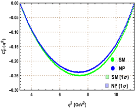
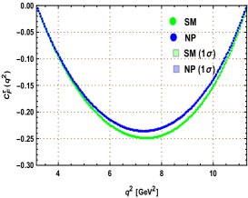
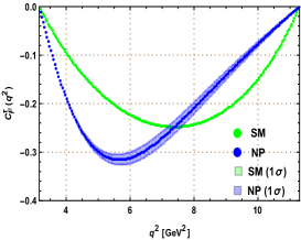
Figure 7: $q^{2}$ dependence of the convexity parameter of $\Sigma_{b}\to\Sigma_{c}\tau^{-}\bar{\nu}_{\tau}$ process. The description of couplings is same as Fig. 2.

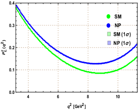
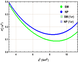
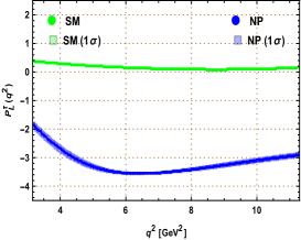
Figure 8: $q^{2}$ dependence of the longitudinal polarisation asymetry of $\Sigma_{b}\to\Sigma_{c}\tau^{-}\bar{\nu}_{\tau}$ process. The description of couplings is the same as Fig. 2.

The convexity parameter $C_{F}^{\tau}$, on the other hand, exhibits a notably large deviation from the SM prediction in the presence of $(C_{lequ}^{(1)},C_{ledq})$, while a moderate deviation is observed with $(C_{lq}^{(3)},C_{ledq})$. The details of the $q^{2}$ behavior is shown in Fig. 7.

Much like the convexity parameter $C_{F}^{\tau}$, the polarization asymmetry, depicted in Fig. 8, shows a significant departure from the SM prediction under the influence of $(C_{lequ}^{(1)},C_{ledq})$, while a more distinctive deviation is observed with $(C_{lq}^{(3)},C_{ledq})$.

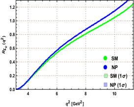
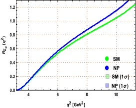
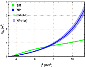
Figure 9: $q^{2}$ behavior of the branching fraction ratio of $\Sigma_{b}\to\Sigma_{c}\tau^{-}\bar{\nu}_{\tau}$. The description of couplings is same as Fig. 2.

We further investigate the $q^{2}$-dependence of the lepton non-universality observable, as shown in Fig. 9. A pronounced deviation from the SM prediction is observed at large $q^{2}$ values, most prominently in the right panel. Conversely, in the low $q^{2}$ region, the deviation from the SM is minimal. Interestingly, such discrepancies are absent in the other two scenarios: in the left panel, the predictions align closely with the SM, while in the middle panel, a measurable deviation from the SM prediction is observed within the range $q^{2}\in[7,11.3]$ GeV², suggesting potential contributions from new physics.

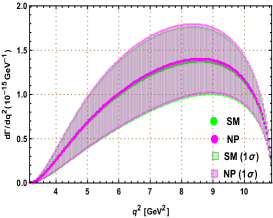
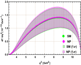
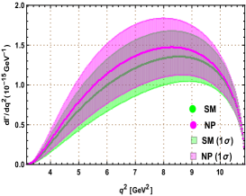
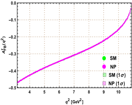
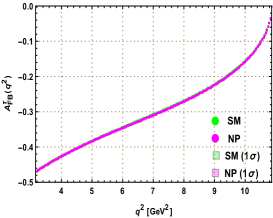
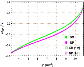
Figure 10: The $q^{2}$ behavior of the branching ratio and forward-backward asymmetry of $\Sigma_{b}\to\Sigma_{c}^{*}\tau^{-}\bar{\nu}_{\tau}$ process. The description of couplings is the same as Fig. 2.

V.3 Analysis of $\Sigma_{b}\to\Sigma_{c}^{*}\tau^{-}\bar{\nu}_{\tau}$ Process

Here, we will discuss the $\Sigma_{b}\to\Sigma_{c}^{*}\tau^{-}\bar{\nu}_{\tau}$ decay observables in the presence of NP couplings. Our analysis on the $q^{2}$ behavior are discussed below.

In the presence of the 2D operators, the branching ratio remains consistent with the SM prediction. On the other hand, the forward-backward asymmetry does not exhibit a zero-crossing point in any of the scenarios. Notably, the couplings $(C_{lequ}^{(1)},C_{ledq})$ display a distinction both in the SM and within the SMEFT formalism. The rest of the scenarios are almost consistent with the SM prediction. This is presented in Fig. 10.

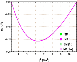
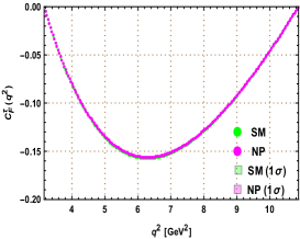
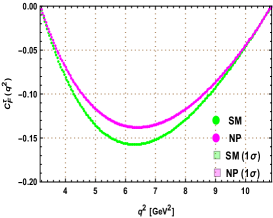
Figure 11: Behavior of convexity parameter. The description of couplings is the same as Fig. 2.

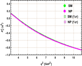
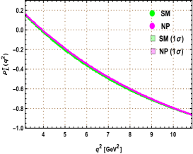
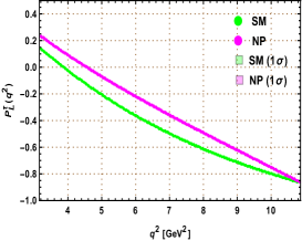
Figure 12: Behavior of $P_{L}^{\tau}(q^{2})$ of $\Sigma_{b}\to\Sigma_{c}^{*}\tau^{-}\bar{\nu}_{\tau}$ channel. The description of couplings is the same as Fig. 2.

The convexity parameter $C_{F}^{\tau}$ shows a significant deviation from the SM prediction when the couplings $(C_{lequ}^{(1)},C_{ledq})$ are present, whereas no new physics contribution is seen with the other two scenarios. The detailed $q^{2}$ behavior is presented in Fig. 11.

In Fig. 12, we observed that the NP sensitivity allows noticeable discrepancies from the SM contribution with the simultaneous presence of $C_{lequ}^{(1)}$ and $C_{ledq}$ couplings.

In the analysis of the lepton non-universality observable, as illustrated in Fig. 13, a measurable difference is observed in the presence of the new physics couplings $(C_{lequ}^{(1)},C_{ledq})$). However, in the presence of other scenarios i.e $(C_{lq}^{(3)},C_{lequ}^{(1)})$ and $(C_{lq}^{(3)},C_{ledq})$, a modest departure is seen in the higher $q^{2}$ region.

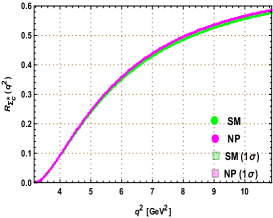
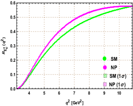
Figure 13: The $q^{2}$ dependent braching fraction ratio of $\Sigma_{b}\to\Sigma_{c}^{*}\tau^{-}\bar{\nu}_{\tau}$ decay channel. The description of couplings is the same as Fig. 2

VI Conclusion

Motivated by the anomalies observed in charged-current mediated $b\to c\ell\nu$ transitions, we have conducted a comprehensive analysis of the exclusive semileptonic $b$-baryonic decay modes $\Sigma_{b}\to\Sigma_{c}^{(*)}\tau^{-}\bar{\nu}_{\tau}$ and $\Xi_{b}\to\Xi_{c}\tau^{-}\bar{\nu}_{\tau}$ within the framework of the SMEFT approach. These decay modes provide a crucial testing ground for probing NP effects. Using the Weak Effective Theory Lagrangian to describe $b\to c\ell\nu$ transitions, we established explicit correlations between the NP couplings and SMEFT Wilson coefficients. In this context, the SMEFT operators responsible for generating $b\to c\tau\nu_{\tau}$ transitions also induce LEFT operators relevant to $b\to s\tau^{+}\tau^{-}$ and $b\to s\nu\nu$ processes. This dual impact emphasizes the interconnected nature of these decay channels in the presence of NP contributions.

For the NP analysis, we constrain the parameter space of the SMEFT couplings, utilizing the experimental data on several key observables, including $R_{D^{(*)}}$, $P_{\tau}(D^{*})$, $F_{L}(D^{*})$, $R_{\Lambda_{c}}$, $\text{BR}(B\to K^{(*)}\nu\bar{\nu})$, $\text{BR}(B_{s}\to\tau^{+}\tau^{-})$, and $\text{BR}(B\to K\tau\tau)$. For our analysis, we assumed the NP couplings to be real. Both 1D and 2D scenarios for the SMEFT couplings were initially considered using the new Wilson coefficients $C_{lq}^{(3)}$, $C_{lequ}^{(1)}$, and $C_{ledq}$. However, we found that the contributions of the 1D scenarios were negligible and, therefore, we have not included them in our analysis.

We conducted a detailed examination of the impact of various 2D NP couplings, such as $(C_{lq}^{(3)},C_{lequ}^{(1)})$, $(C_{lq}^{(3)},C_{ledq})$, and $(C_{lequ}^{(1)},C_{ledq})$, on the branching fractions and angular observables, including lepton polarization asymmetry, forward-backward asymmetry, convexity parameter, and the lepton non-universality observable of the $b$-baryonic decay modes $\Sigma_{b}\to\Sigma_{c}^{(*)}\tau^{-}\bar{\nu}_{\tau}$ and $\Xi_{b}\to\Xi_{c}\tau^{-}\bar{\nu}_{\tau}$. These results highlight the sensitivity of these processes to NP effects and their potential to complement the insights gained from mesonic decays.

Our results reveal a significant sensitivity to NP effects in $\Xi_{b}\to\Xi_{c}\tau\nu$ and $\Sigma_{b}\to\Sigma_{c}^{(*)}\tau\bar{\nu}$, with the couplings $(C_{lequ}^{(1)},C_{ledq})$ yielding more pronounced deviations from the SM predictions than the other couplings. However, the coupling $(C_{lq}^{(3)},C_{ledq})$ exhibits a moderate deviation in the high $q^{2}$ region for the convexity parameter, lepton polarization asymmetry, and the lepton non-universality observable of the $\Sigma_{b}\to\Sigma_{c}\tau\bar{\nu}$ process.

In summary, this detailed analysis of the $b$-baryonic decay modes $\Sigma_{b}\to\Sigma_{c}^{(*)}\tau^{-}\bar{\nu}_{\tau}$ and $\Xi_{b}\to\Xi_{c}\tau^{-}\bar{\nu}_{\tau}$ reveals that the associated observables, both within the Standard Model and in new physics scenarios, fall within the experimental reach of current facilities such as Belle-II and LHCb. Precise measurements of these observables will offer valuable insights into the impact of new physics on exclusive $b$-baryonic decays mediated by $b\to c\ell\nu$ transitions.

VII Acknowledgement

DP would like to acknowledge the support of the Prime Minister’s Research Fellowship, Government of India. MKM acknowledges the financial support from IoE PDRF, University of Hyderabad. RM would like to acknowledge the University of Hyderabad IoE project grant no. RC1-20-012.

References

- (1) J. P. Lees et al., “Evidence for an excess of decays,” Phys. Rev. Lett., vol. 109, p. 101802, 2012.
- (2) J. P. Lees et al., “Measurement of an Excess of Decays and Implications for Charged Higgs Bosons,” Phys. Rev. D, vol. 88, no. 7, p. 072012, 2013.
- (3) M. Huschle et al., “Measurement of the branching ratio of relative to decays with hadronic tagging at Belle,” Phys. Rev. D, vol. 92, no. 7, p. 072014, 2015.
- (4) Y. Sato et al., “Measurement of the branching ratio of relative to decays with a semileptonic tagging method,” Phys. Rev. D, vol. 94, no. 7, p. 072007, 2016.
- (5) A. Abdesselam et al., “Measurement of the lepton polarization in the decay ,” 8 2016.
- (6) G. Caria et al., “Measurement of and with a semileptonic tagging method,” Phys. Rev. Lett., vol. 124, no. 16, p. 161803, 2020.
- (7) R. Aaij et al., “Measurement of the ratio of branching fractions ,” Phys. Rev. Lett., vol. 115, no. 11, p. 111803, 2015. [Erratum: Phys.Rev.Lett. 115, 159901 (2015)].
- (8) R. Aaij et al., “Measurement of the ratio of the and branching fractions using three-prong -lepton decays,” Phys. Rev. Lett., vol. 120, no. 17, p. 171802, 2018.
- (9) Y. S. Amhis et al., “Averages of b-hadron, c-hadron, and -lepton properties as of 2021,” Phys. Rev. D, vol. 107, no. 5, p. 052008, 2023.
- (10) S. Fajfer, J. F. Kamenik, and I. Nisandzic, “On the Sensitivity to New Physics,” Phys. Rev. D, vol. 85, p. 094025, 2012.
- (11) J. F. Kamenik and F. Mescia, “ Branching Ratios: Opportunity for Lattice QCD and Hadron Colliders,” Phys. Rev. D, vol. 78, p. 014003, 2008.
- (12) S. Aoki et al., “Review of lattice results concerning low-energy particle physics,” Eur. Phys. J. C, vol. 77, no. 2, p. 112, 2017.
- (13) S. Hirose et al., “Measurement of the lepton polarization and in the decay ,” Phys. Rev. Lett., vol. 118, no. 21, p. 211801, 2017.
- (14) P. Asadi, M. R. Buckley, and D. Shih, “Asymmetry Observables and the Origin of Anomalies,” Phys. Rev. D, vol. 99, no. 3, p. 035015, 2019.
- (15) A. K. Alok, D. Kumar, S. Kumbhakar, and S. U. Sankar, “ polarization as a probe to discriminate new physics in ,” Phys. Rev. D, vol. 95, no. 11, p. 115038, 2017.
- (16) I. Ray and S. Nandi, “Test of new physics effects in decays with heavy and light leptons,” JHEP, vol. 01, p. 022, 2024.
- (17) R. Aaij et al., “Measurement of the ratio of branching fractions /,” Phys. Rev. Lett., vol. 120, no. 12, p. 121801, 2018.
- (18) R. Dutta and A. Bhol, “ semileptonic decays within the standard model and beyond,” Phys. Rev. D, vol. 96, no. 7, p. 076001, 2017.
- (19) T. Aaltonen et al., “Observation and mass measurement of the baryon ,” Phys. Rev. Lett., vol. 99, p. 052002, 2007.
- (20) V. M. Abazov et al., “Direct observation of the strange baryon ,” Phys. Rev. Lett., vol. 99, p. 052001, 2007.
- (21) R. Aaij et al., “Precision measurement of the mass and lifetime of the baryon,” Phys. Rev. Lett., vol. 113, p. 032001, 2014.
- (22) R. Aaij et al., “Measurement of the and baryon lifetimes,” Phys. Lett. B, vol. 736, pp. 154–162, 2014.
- (23) R. Aaij et al., “Studies of beauty baryon decays to and final states,” Phys. Rev. D, vol. 89, no. 3, p. 032001, 2014.
- (24) R. Aaij et al., “Precision Measurement of the Mass and Lifetime of the Baryon,” Phys. Rev. Lett., vol. 113, no. 24, p. 242002, 2014.
- (25) R. Aaij et al., “Evidence for the strangeness-changing weak decay ,” Phys. Rev. Lett., vol. 115, no. 24, p. 241801, 2015.
- (26) R. Aaij et al., “Observation of the decay ,” Phys. Rev. Lett., vol. 118, no. 7, p. 071801, 2017.
- (27) R. Aaij et al., “Observation of the decay,” Phys. Lett. B, vol. 772, pp. 265–273, 2017.
- (28) T. Aaltonen et al., “Measurement of the masses and widths of the bottom baryons and ,” Phys. Rev. D, vol. 85, p. 092011, 2012.
- (29) R. Aaij et al., “Observation of Two Resonances in the Systems and Precise Measurement of and properties,” Phys. Rev. Lett., vol. 122, no. 1, p. 012001, 2019.
- (30) H.-W. Ke, N. Hao, and X.-Q. Li, “Revisiting and weak decays in the light-front quark model,” Eur. Phys. J. C, vol. 79, no. 6, p. 540, 2019.
- (31) D. Ebert, R. N. Faustov, and V. O. Galkin, “Semileptonic decays of heavy baryons in the relativistic quark model,” Phys. Rev. D, vol. 73, p. 094002, 2006.
- (32) R. L. Singleton, “Semileptonic baryon decays with a heavy quark,” Phys. Rev. D, vol. 43, pp. 2939–2950, 1991.
- (33) M. A. Ivanov, V. E. Lyubovitskij, J. G. Korner, and P. Kroll, “Heavy baryon transitions in a relativistic three quark model,” Phys. Rev. D, vol. 56, pp. 348–364, 1997.
- (34) M. A. Ivanov, J. G. Korner, V. E. Lyubovitskij, and A. G. Rusetsky, “Charm and bottom baryon decays in the Bethe-Salpeter approach: Heavy to heavy semileptonic transitions,” Phys. Rev. D, vol. 59, p. 074016, 1999.
- (35) H.-W. Ke, X.-H. Yuan, X.-Q. Li, Z.-T. Wei, and Y.-X. Zhang, “ and weak decays in the light-front quark model,” Phys. Rev. D, vol. 86, p. 114005, 2012.
- (36) W. Wang, F.-S. Yu, and Z.-X. Zhao, “Weak decays of doubly heavy baryons: the case,” Eur. Phys. J. C, vol. 77, no. 11, p. 781, 2017.
- (37) N. Rajeev, R. Dutta, and S. Kumbhakar, “Implication of anomalies on semileptonic decays of and baryons,” Phys. Rev. D, vol. 100, no. 3, p. 035015, 2019.
- (38) Y. Sakaki, M. Tanaka, A. Tayduganov, and R. Watanabe, “Testing leptoquark models in ,” Phys. Rev. D, vol. 88, no. 9, p. 094012, 2013.
- (39) C. Bobeth, M. Misiak, and J. Urban, “Photonic penguins at two loops and dependence of ,” Nucl. Phys. B, vol. 574, pp. 291–330, 2000.
- (40) C. Bobeth, A. J. Buras, F. Kruger, and J. Urban, “QCD corrections to , , and in the MSSM,” Nucl. Phys. B, vol. 630, pp. 87–131, 2002.
- (41) A. J. Buras, J. Girrbach-Noe, C. Niehoff, and D. M. Straub, “ decays in the Standard Model and beyond,” JHEP, vol. 02, p. 184, 2015.
- (42) W. Altmannshofer, A. J. Buras, D. M. Straub, and M. Wick, “New strategies for New Physics search in , and decays,” JHEP, vol. 04, p. 022, 2009.
- (43) J. Aebischer, A. Crivellin, M. Fael, and C. Greub, “Matching of gauge invariant dimension-six operators for and transitions,” JHEP, vol. 05, p. 037, 2016.
- (44) R. Dutta, A. Bhol, and A. K. Giri, “Effective theory approach to new physics in b → u and b → c leptonic and semileptonic decays,” Phys. Rev. D, vol. 88, no. 11, p. 114023, 2013.
- (45) H. 2022, “Preliminary average of and for Winter 2023,” 2022. https://hflav-eos.web.cern.ch/hflav-eos/semi/winter23prel/html/RDsDsstar/RDRDs.html.
- (46) A. Abdesselam et al., “Measurement of the polarization in the decay ,” in 10th International Workshop on the CKM Unitarity Triangle, 3 2019.
- (47) R. Aaij et al., “Observation of the decay ,” Phys. Rev. Lett., vol. 128, no. 19, p. 191803, 2022.
- (48) I. Adachi et al., “Evidence for B+→K+¯ decays,” Phys. Rev. D, vol. 109, no. 11, p. 112006, 2024.
- (49) J. Grygier et al., “Search for decays with semileptonic tagging at Belle,” Phys. Rev. D, vol. 96, no. 9, p. 091101, 2017. [Addendum: Phys.Rev.D 97, 099902 (2018)].
- (50) R. Aaij et al., “Search for the decays and ,” Phys. Rev. Lett., vol. 118, no. 25, p. 251802, 2017.
- (51) J. P. Lees et al., “Search for at the BaBar experiment,” Phys. Rev. Lett., vol. 118, no. 3, p. 031802, 2017.