Department of Physics

Scattering waveforms for Kerr black holes from the soft expansion

Theoretical physics

Professors:
Paolo Pani
Vittorio Del Duca
Riccardo Gonzo

Students:

Damiano Barcaro

 
Academic Year 2023/2024

Abstract

In this thesis, I will study the classical scattering problem of two Kerr black holes in general relativity with novel quantum field theory techniques in the Post-Minkowskian (PM) expansion, generalizing the subleading soft theorem to the case of spinning particles. The leading order term in the soft expansion is uniquely determined by the universal Weinberg pole, but the subleading one depends on the angular momentum of the external particles and receives a new spin corrections for classically spinning black holes. Using this approach, I will compute the gravitational Compton amplitude, both in the quantum and classical theory. I will then compute the tree-level five-point amplitude of two spinning point particles emitting a graviton, using the spinor-helicity formalism combined with the soft expansion. Finally, I will use the KMOC formalism to derive the analytic time-domain waveform for the scattering of two Kerr black holes at leading order in the PM expansion.

.

1 Introduction

The advent of gravitational-wave (GW) science [1, 2, 3] has already revolutionized multiple domains of astronomy, cosmology, and particle physics. However, this is merely a glimpse of the vast potential yet to be unlocked [4, 5].
Future developments of GW science require a robust theoretical framework to support precision calculations of GW signals. Over the next decade, both space- and ground-based observatories are expected to detect and characterize millions of merger events annually, with sensitivity far surpassing that of current LIGO/Virgo facilities (see, e.g., [6, 7, 8, 9, 10]). In particular, these progresses will address the need for high precision in upcoming LIGO-Virgo-KAGRA (LVK) runs, in space-based detectors such as LISA [4], and in future ground-based detectors such as LIGO-India [11], Cosmic Explorer [12] and Einstein Telescope [13]. To fully exploit the discovery potential of these increasingly sensitive detectors, the development of high-precision waveform models will be essential [4, 14, 15, 5, 16].

One of the key challenges will be advancing the theoretical modeling of compact binary coalescences to produce accurate gravitational waveforms.

Figure 1: The GW150914 signal observed at the Hanford observatory. The three stages of the coalescing process are indicated. The lower plot shows the velocity of the components as function of their spatial separation. Figure reproduced from Ref. [1].

The theoretical modeling of gravitational-wave (GW) sources poses significant challenges due to the presence of multiple physical scales, which are intricately coupled through the nonlinear framework of general relativity. Interestingly, these very
complications —nonlinearity and multi-scale dynamics— are analogous to the challenges that spurred groundbreaking advancements in quantum field theory (QFT) over the past few decades.
The modern scattering amplitudes program, born from these efforts, has uncovered deep mathematical structures in both gauge theory and gravity. This has not only provided new physical insights but also led to highly efficient computational methods and inspired the development of more ambitious theoretical frameworks.
For recent overviews, see [17, 18, 19, 20, 21]. Particularly noteworthy is the seminal work [22], which introduced nonrelativistic effective field theory (EFT) concepts from particle physics into the worldline approach for binary dynamics. This innovation has led to several landmark results, with recent developments thoroughly documented in the Snowmass White Paper on NRGR [23].

Scattering amplitudes are gauge-invariant, universal objects that compactly and analytically encode the perturbative dynamics of point particles. They offer numerous advantages: often expressed through concise analytic formulas, they provide deep physical insights and benefit from a flexible, scalable formalism. This adaptability makes it straightforward to incorporate subleading contributions or new physics, such as spin, tidal effects, or extensions beyond general relativity.
However, there are notable challenges. To connect the mathematical formalism of scattering amplitudes with the physics of bound black hole systems, a scatter-to-bound map is required. Moreover, a resummation scheme is necessary, as the perturbative results derived from amplitude methods must be resummed to accurately reflect the non-perturbative nature of bound systems.

The Parke-Taylor formula [24] dramatically simplified gluon scattering calculations, reducing pages of Feynman diagrams to a concise half-line expression. This landmark result showcased the profound importance of uncovering the theoretical structures underlying scattering amplitudes. In recent decades, this field has experienced major advances due to two parallel developments.
The first is the emergence of novel methods that reformulate quantum field theory (QFT) without relying on explicit quantum fields, instead focusing directly on physical observables. These ”on-shell methods,” revitalized by twistor string theory ideas [25, 26, 27, 28], have become highly efficient tools for both tree-level [29] and loop-level [30, 31, 32, 33] calculations in gauge and gravity theories. For comprehensive overviews, see [34, 35, 36, 37, 38].
The second development is a radically new insight into gravity: gravitational scattering amplitudes, $\mathcal{M}_{\rm gravity}$, can be expressed as a ”double copy” of gauge theory amplitudes, $\mathcal{M}_{\rm gauge}$ [39, 40].

$${\cal M}_{\rm gauge}\times{\cal M}_{\rm gauge}\sim{\cal M}_{\rm gravity}\,.$$ (1.1)

This correspondence has provided a powerful bridge between gauge and gravity theories, revealing deep structural connections between the two.

The new approach, leveraging tools from theoretical high-energy physics, aims to complement, and has significantly benefited from, decades of successful efforts using traditional methods to solve the relativistic two-body. Some of the most remarkable approaches are the post-Newtonian (PN) approximation [41, 42, 43, 44, 45, 46, 47, 48, 49], the gravitational self-force (GSF) formalism [50, 51], the effective-one-body (EOB) framework [52, 53], and the nonrelativistic general relativity (NRGR) approach [22]. Other important frameworks include the post-Minkowskian (PM) approximation [54, 55, 56, 57, 58, 59, 60, 61, 62, 63], and numerical relativity (NR) methods [64, 65, 66].
It’s important to remark that amplitudes demonstrate strong synergies with PN and GSF approaches, enhancing their utility across various frameworks, see Fig. (2).

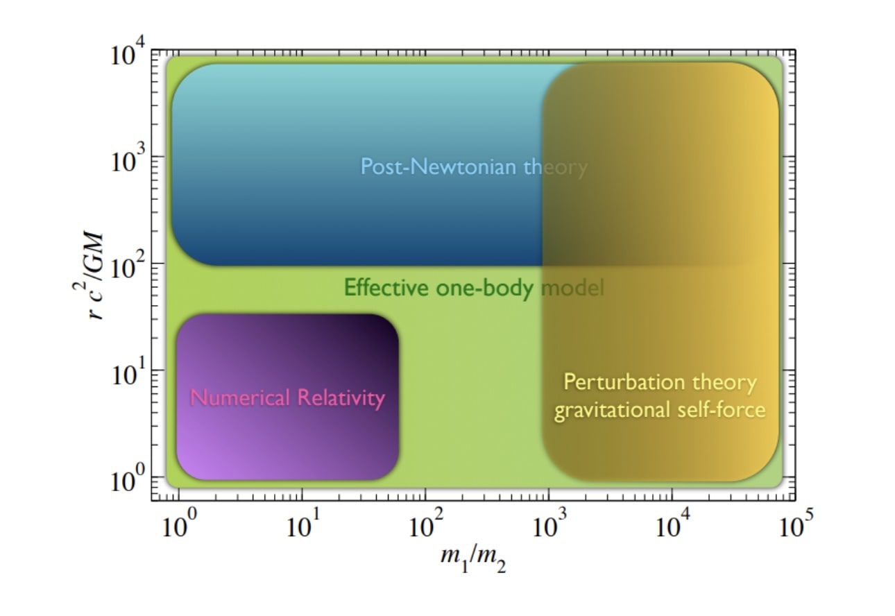
Figure 2: To model accurately the entire parameter space of the two-body dynamics, various communities need to work together: Gravitational self-force (GSF), Post-Minkowskian (PM), Post-Newtonian (PN) and numerical relativity (NR). In the above figure the validity of the different methods producing gravitational wave templates in a typical BBH system is shown. Figure reproduced from Ref. [67].

Leveraging newly developed tools from theoretical particle physics offers significant advantages for gravitational wave physics. First, the structure of perturbation theory is greatly streamlined by using special relativity, on-shell methods, and the double-copy framework, resulting in compact expressions that expose the underlying theoretical structures. Second, advanced techniques and a well-established knowledge base for loop integration in quantum field theory —refined over decades for collider physics—can be directly applied. This includes integration-by-parts systems [68, 69, 70] and the use of differential equations [71, 72, 73, 74, 75, 76, 77], which are now highly developed for efficient loop calculations. Finally, effective field theory (EFT) methods are well-suited for systematically addressing different contributions in the classical limit, allowing for targeted and precise predictions across a range of processes. Figure 4 illustrates the application of these tools in GW physics.

Figure 3: Map of perturbative corrections to Newton’s potential, where $G$ is Newton’s constant and $v$ is the relative velocity of the binary constituents. New results through $O(G^{4})$ were recently obtained using QFT tools (red box). They are valid to all orders in velocity, and overlap with the state-of-the-art from the PN expansion (dark triangle) and the contributions required by future detectors (light triangle) (see, e.g.,  [6, 7, 8, 9, 10]). Figure reproduced from Ref. [78].

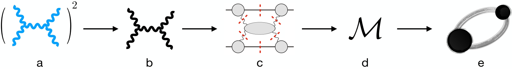
Figure 4: (top) Classical binary dynamics is encoded in scattering amplitudes of massive particles (thick lines) interacting through gravitons (wavy lines): (A) four-point scattering encodes higher-order corrections to conservative binary dynamics, (B) five-point scattering encodes radiative effects due to graviton emission, and (C) higher-dimension operators (solid circle) encode tidal deformation of neutron stars. Spinning black holes can be described by higher-spin representations in QFT.    (bottom) A sample calculational pipeline using the tools of theoretical high-energy physics: Starting from tree-level gauge theory amplitudes (a), corresponding gravitational amplitudes (b) are obtained using the double-copy. These are then fused into loop amplitudes (c) using generalized unitarity. The integrated amplitude (d) is obtained using advanced multiloop integration methods developed in high-energy physics, in combination with EFT. The amplitude can then be mapped, using a variety of methods, to the EOB Hamiltonian used for producing waveforms (e). The classical limit is applied at every stage, leading to vast simplifications. Figure reproduced from Ref. [78].

In addition to providing state-of-the-art predictions, the new approach using particle physics tools seeks to uncover theoretical structures that emerge in the classical limit of scattering amplitudes. Some of these structures may be well-known in particle physics but remain hidden in traditional treatments of the two-body problem in general relativity. Others may originate in the classical regime and have yet to be fully explored from the perspective of quantum field theory. Key examples include universality in the high-energy limit, the interaction between conservative and dissipative effects, nonperturbative connections to classical solutions, and the development of perturbation theory in curved backgrounds.
Ultimately, scattering amplitudes serve as powerful tools for both understanding and precisely modeling gravitational wave sources, in much the same way as they are used to describe interactions between fundamental particles.

Classical Limit

The correspondence principle asserts that classical physics arises as the macroscopic limit of quantum theory, where conserved quantities (charges) such as mass, electric charge, spin, and orbital angular momentum become large. Perturbations around such macroscopic configurations, which are subleading relative to the large charges, can be systematically included and naturally interpreted as quantum corrections.
In the context of gravitational waves, the classical limit of scattering amplitudes is characterized by two key properties that distinguish compact binaries from their quantum counterparts:

• Large angular momentum: Bound compact objects, such as black holes or neutron stars, exhibit large angular momentum $J\gg\hbar$, in contrast to quantum bound states where $J\sim\hbar\equiv 1$.

• Large gravitational charges: Compact objects possess significantly large gravitational charges, for example, black holes or neutron stars have $M_{\odot}/M_{\rm Planck}\sim 10^{38}$, compared to the much smaller ratio of $e/Q_{\rm Planck}\sim 10^{-1}$ for the electric charges of elementary particles. Here, $M_{\odot}$ represents the solar mass and $e$ the electron charge, while $M_{\rm Planck}$ and $Q_{\rm Planck}$ are the Planck mass and Planck charge, respectively.

In other words, for a system of two gravitationally interacting spinless bodies with masses $m_{1}$ and $m_{2}$, the classical regime emerges when the angular momentum $J\gg\hbar$ and the masses $m_{1},m_{2}\gg M_{\rm Planck}$. This regime corresponds to the condition where the de Broglie wavelength $\lambda$ of the particles is much smaller than the separation between the particles $|\mathbf{b}|$, which is conjugate to the momentum transfer $\mathbf{q}$. Thus, the classical physics regime is characterized by momentum transfer being much smaller than the incoming momenta, $|\mathbf{p}|\gg|\mathbf{q}|$.
Other charges that may characterize classical particles follow similar scaling behavior in the classical limit, e.g. : the spin $S$ and finite size $R$ scale as $|\mathbf{q}|R\sim\mathcal{O}(1)$ and $|\mathbf{q}||\mathbf{S}|\sim m_{1,2}$, respectively.
These scalings are consistent with the classical form of Newton’s potential, where $|\mathbf{b}|\gg Gm$, and they impose constraints on the general structure of four-point scattering amplitudes and the generating functions for observable quantities.

Another perspective on the classical limit is presented in [79], which is commonly referred to as the KMOC formalism. The details of this formalism will be elaborated in Sec. 3.

A significant implication of the classical limit is that loop amplitudes involving massive particles can contain classical contributions. Importantly, this classical limit can be applied at the initial stages of calculations, leading to substantial simplifications before the integration process. This approach allows for the computation of amplitudes that would otherwise be impractical to evaluate if quantum effects were included from the outset.

Recent insights have highlighted a remarkable connection between the soft limit in quantum theories and memory effects in classical dynamics [80]. This relationship can be explored within the KMOC formalism by examining the radiated momentum. In the long-wavelength limit, the scattering amplitude associated with radiation simplifies to a soft factor multiplied by a lower-point amplitude, effectively recovering the impulse [81].
Classically, this impulse represents the ”memory” of a step-change in the field, characterized by its very low-frequency Fourier components. More broadly, the KMOC formalism elucidates a rich interplay between classical physics, soft or low-frequency radiation, and scattering amplitudes [82, 83, 84, 85, 86].

A comprehensive overview of the latest state-of-the-art predictions can be found in Ref. [78].

This thesis is organized as follows: in the first chapter Sec. 2 I will describe the spinor-helicity formalism, that I will use throughout the entirety of this work. Thanks to this formalism many breakthroughs in particle physics were made in the previous decades, furthermore the application of this formalism to gravity scattering amplitudes led to many elegant results.

In the second chapter Sec. 3 I will introduce the aforementioned KMOC formalism, describing its intricacies and providing a general method to compute observables.

In the third chapter (Sec. 4), I will begin computing amplitudes, starting with the simplest case: three-point amplitudes. I will first calculate the massless and equal-mass three-point amplitudes in a quantum framework, and then derive their classical counterparts. I will also provide a straightforward method for computing the classical (infinite-spin) limit.

In the fourth chapter Sec. 5 I will discuss a general method to obtain higher-point amplitudes, introducing the BCFW recursion relations. Furthermore, I will introduce the soft recursion relations to compute $(n+1)$-amplitudes with one additional external graviton starting from the corresponding $n$-amplitudes.

In the fifth chapter Sec. 6 I will apply the soft recursion relations of Sec. 4 to the three-point amplitudes obtained in Sec. 5 to compute the gravitational Compton amplitude, both in the spinless and spinning black holes cases. I will then evaluate their classical counterpart. At the end of this chapter I will also introduce a classical version of the soft recursion relations to obtain higher-point classical amplitudes from lower-point ones in a purely classical setting.

In the sixth chapter Sec. 7 I will first use the BCFW recursion relations introduced in Sec. 4 to compute the 2-to-2 black holes scattering amplitudes without the emission of radiation. I will then use the soft recursions to compute the five-point amplitude, and then take its classical limit.

In the seventh chapter Sec. 8 I will use the formalism discussed in Sec. 3 to compute the waveform at leading order for the black holes scattering with emission of radiation both in the spinning and spinless cases.

2 Scattering amplitudes

Scattering amplitudes are central to particle physics: their modulus squared is the most important ingredient in the computation of cross sections. The traditional approach to the computation of an un-polarized cross section is to square the amplitude and sum over the polarization of the external states, averaging over the initial ones. The outcome is an expression in terms of Mandelstam invariants and masses.
The traditional workflow is based on the following steps: we choose the irreducible representations of the Poincaré group, whom are subsequently associated to the fields of the particle present in the theory of interest; following Gell-Mann totalitarian principle we now construct the most general Lagrangian. From this Lagrangian we extract the Feynman rules and use them to obtain the Feynman diagrams. We now have all ingredients necessary to evaluate any scattering amplitude, which is finally squared and integrated in order to get the cross section which can be compared with the experimental data. The bottleneck in this procedure happens when we square the amplitude, as if we are presented with n Feynman diagrams, $n^{2}$ terms will appear in the cross section. The computation quickly becomes intractable as the number of external particles grows, even with state-of-the-art computers.
Fixing the polarizations of the external particles, i.e. for massless particles the helicities, improves a lot the computation: for a given helicity configuration the amplitude is just a complex number; furthermore, different helicity configurations do not interfere with each other. Therefore if the amplitude has n helicity configurations, the cross section is simply the sum of the n squared contributions at fixed helicity. As a final bonus, different helicity configurations are often related by charge conjugation or parity, greatly reducing the number or configurations needed to be computed.
Finally, while Feynman diagrams are local in space-time, they are off-shell and not gauge invariant (individually). The ultimate advantage of amplitudes is that they are on-shell and gauge invariant objects. In fact, one might want to re-think QFTs starting from the fundamental pillars quantum mechanics and special relativity.

2.1 The Little group

Amplitudes scatter particles. Let us see then how we can characterize quantum one-particle states. I will mainly follow the work presented in Ref. [87, 88].
Physical states are represented by rays $\mathcal{R}$ in Hilbert space, i.e. by normalized vectors $|\psi\rangle$ with $\langle\psi|\psi\rangle=1$, where we identify states $|\psi\rangle$ up to an arbitrary overall phase $e^{i\gamma}$, with $\gamma\in\mathbb{R}$, i.e. $|\psi\rangle$ and $|\psi^{\prime}\rangle=e^{i\gamma}|\psi\rangle$ belong to the same ray $\mathcal{R}$.
Physical observables A are represented by Hermitian operators. A state $|\psi\rangle$ has definite value $\alpha$ for the observable A if $|\psi\rangle$ is an eigenvector of A, with $A|\psi\rangle=\alpha|\psi\rangle,\,\alpha\in\mathbb{R}$.
A transformation between two different observers O and O’ who observe the same system is a symmetry transformation. In such a case, if O observes the states $|\psi_{i}\rangle\in\mathcal{R}_{i}$, and O’ the states $|\psi^{\prime}_{i}\rangle\in\mathcal{R}^{\prime}_{i}$, then the transition probabilities, $\mathcal{P}\left(\mathcal{R}_{1}\rightarrow\mathcal{R}_{2}\right)\equiv\left|\langle\psi_{1}|\psi_{2}\rangle\right|^{2}$, are conserved, i.e. $\mathcal{P}\left(\mathcal{R}_{1}\rightarrow\mathcal{R}_{2}\right)=\mathcal{P}\left(\mathcal{R}^{\prime}_{1}\rightarrow\mathcal{R}^{\prime}_{2}\right)$.
Wigner showed that the operator $\mathcal{U}$ which implements the symmetry transformation must be unitary and linear (or anti-unitary and anti-linear). In particular, transformations which are continuously connected to the identity are represented by a linear unitary operator $\mathcal{U}$.
The symmetry transformations $\Lambda$ form a group, and the corresponding operators $\mathcal{U}$ acting on the rays mimic the group structure. In fact, one can show that

$$\mathcal{U}(\Lambda_{1})\mathcal{U}(\Lambda_{2})=e^{i\phi\left(\Lambda_{1},\Lambda_{2}\right)}\mathcal{U}(\Lambda_{1},\Lambda_{2}).$$ (2.1)

If $\phi=0$, then the $\mathcal{U}(\Lambda)$ provide a representation of $\Lambda$. For $\phi\neq 0$, they provide a projective representation.

The tenets of any QFT, even on-shell, are quantum mechanics and special relativity, therefore any transformation under the Poincaré group P must be symmetry transformations. The Poincaré group itself is the minimal subgroup of the affine group which includes all translations and Lorentz transformations. More precisely, it is a semidirect product of the spacetime translations group and the Lorentz group. In particular under the action of a Poincaré transformation, a vector $x^{\mu}$ transforms as $x^{\mu}\xrightarrow{P}\Lambda^{\mu}_{~{}\nu}x^{\nu}+b^{\mu}$, with $\left(det\Lambda\right)^{2}=1$.

One-particle states (1PS) are classified by the irreducible representations of the Poincaré group, which, Wigner showed, can be classified by the irreducible representations of the little group, i.e. the subgroup of transformations which leave the momentum $k$ invariant: $W^{\mu}_{~{}\nu}k^{\nu}=k^{\mu}$.
We want to classify our 1PS by a maximal set of commuting operators, whose eigenvalues will be our quantum numbers, in order to identify the states univocally. We recall that commuting operators can be simultaneously diagonalized. The components of the momentum commute with each other, so their eigenvalues can be chosen to be our first quantum number; furthermore, the momentum operator $\text{P}^{\mu}$ commutes with the operator $\text{P}^{2}$, which will be associated to the second quantum number. The discrete degrees of freedom (e.g. the helicity, …) will be labeled with $\sigma$.
So the 1PS can be written as $|p;\sigma\rangle$, with $\mathrm{P}^{\mu}|p;\sigma\rangle=p^{\mu}|p;\sigma\rangle$.

Under a general Lorentz transformation $\mathrm{P}^{\mu}$ transforms as a vector:

$$\mathrm{P}^{\mu}\rightarrow\mathrm{P^{\prime}}^{\mu}\equiv\mathcal{U}(\Lambda)\mathrm{P}^{\mu}\mathcal{U}(\Lambda)=\left(\Lambda^{-1}\right)^{\mu}_{~{}\nu}\mathrm{P}^{\nu}=\Lambda^{~{}\mu}_{\nu}\mathrm{P}^{\nu}.$$ (2.2)

The action of $\mathcal{U}(\Lambda)$ on the state $|p;\sigma\rangle$ is to produce an eigenvector of $\mathrm{P}^{\mu}$ with eigenvalue $\Lambda_{p}$. We now might act with $\mathrm{P}^{\mu}$ on the state $\mathcal{U}(\Lambda)|p;\sigma\rangle$:

$$\mathrm{P}^{\mu}\mathcal{U}(\Lambda)|p;\sigma\rangle=\mathcal{U}(\Lambda)\left(\mathcal{U}^{-1}(\Lambda)\mathrm{P}^{\mu}\mathcal{U}(\Lambda)\right)|p;\sigma\rangle=\mathcal{U}(\Lambda)(\Lambda^{-1})_{\nu}^{~{}\mu}\mathrm{P}^{\nu}|p;\sigma\rangle=\Lambda^{\mu}_{~{}\nu}p^{\nu}\mathcal{U}(\Lambda)|p;\sigma\rangle.$$ (2.3)

Therefore $\mathcal{U}(\Lambda)|p;\sigma\rangle$ must be a linear combination of Lorentz-transformed 1PS,

$$\mathcal{U}(\Lambda)|p;\sigma\rangle=C_{\sigma\sigma^{\prime}}(\Lambda,p)|\Lambda p;\sigma^{\prime}\rangle.$$ (2.4)

The crucial point is then to express the coefficients $C_{\sigma\sigma^{\prime}}(\Lambda,p)$ in terms of irreducible representations of the Poincaré group.

The only functions of $p^{\mu}$ which are left invariant by (proper orthochronous) Lorentz transformations are $p^{2}=m^{2}$ and, if $m^{2}>0$, the sign of $p^{0}$. For each $p^{2}$, we can choose a reference momentum $k^{\mu}$ such that $p^{\mu}=L^{\mu}_{~{}\nu}(p;k)k^{\nu}$ and we can define the 1PS as $|p;\sigma\rangle=\mathcal{U}\big{(}L(p;k)\big{)}|k;\sigma\rangle$. Under a general Lorentz transformation, $|p;\sigma\rangle$ transforms in the following way:

$$\mathcal{U}(\Lambda)|p;\sigma\rangle=\mathcal{U}\big{(}\Lambda L(p;k)\big{)}|k;\sigma\rangle=\mathcal{U}\big{(}L(\Lambda p;k)\big{)}\mathcal{U}\big{(}L^{-1}(\Lambda p;k)\Lambda L(p;k)\big{)}|k;\sigma\rangle$$ (2.5)

We now define the transformation $W=L^{-1}(\Lambda p;k)\Lambda L(p;k)$. This transformation maps $k$ to $p=L(p;k)K$, then to $\Lambda p$, then back to $k$, hence it leaves $k^{\mu}$ invariant, i.e. $W^{\mu}_{~{}\nu}k^{\nu}=k^{\mu}$.

As previously mentioned, the subgroup of the Lorentz group composed of the Lorentz maps that leave $k^{\mu}$ invariant is the little group. The action of $W$ on the reference state $|k;\sigma\rangle$ yields a linear combination of reference states,

$$\mathcal{U}\big{(}W(\Lambda,p;k)\big{)}|k;\sigma\rangle=D_{\sigma\sigma^{\prime}}\big{(}W(\Lambda,p;k)\big{)}|k;\sigma^{\prime}\rangle,$$ (2.6)

where the coefficients $D_{\sigma\sigma^{\prime}}$ provide a representation of the little group.

In light of everything shown above, we come back to the original problem in Eq. (2.4):

$$\mathcal{U}(\Lambda)|p;\sigma\rangle =\mathcal{U}\big{(}L(\Lambda p;k)\big{)}\mathcal{U}\big{(}W(\Lambda,p;k)\big{)}|k;\sigma\rangle=$$

$$=D_{\sigma\sigma^{\prime}}\big{(}W(\Lambda,p;k)\big{)}\mathcal{U}\big{(}L(\Lambda p;k)\big{)}|k;\sigma^{\prime}\rangle=D_{\sigma\sigma^{\prime}}\big{(}W(\Lambda,p;k)\big{)}|\Lambda p;\sigma^{\prime}\rangle$$ (2.7)

Thus the issue of determining the coefficients $C_{\sigma\sigma^{\prime}}(\Lambda,p)$ has been reduced to finding the representations $D_{\sigma\sigma^{\prime}}\big{(}W(\Lambda,p;k)\big{)}$ of the little group.

To sum up, a particle is labeled by its momentum and transforms under representations of the little group. Thus an n-point scattering amplitude $\mathcal{M}_{n}$ is labeled by $|p_{i};\sigma_{i}\rangle$, with $i=1\dots n$. Furthermore, Poincaré invariance implies that

$$\mathcal{M}(p_{i};\sigma_{i})=\delta^{D}(p_{1}^{\mu}+\dots+p_{n}^{\mu})M_{n}(p_{i};\sigma_{i}),$$ (2.8)

$$M^{\Lambda}(p_{i};\sigma_{i})=\prod_{i=1}^{n}D_{\sigma_{i}\sigma^{\prime}_{i}}(W)M\big{(}(\Lambda p)_{i};\sigma_{i}\big{)}.$$ (2.9)

In $D$ spacetime dimensions, the little group for massive particles is $SO(D{-}1)$. For massless particles the little group is the the group of Euclidean symmetries in $(D{-}2)$ dimensions. Finite-dimensional representations require choosing all states to have vanishing eigenvalues under these translations, and hence the little group is just $SO(D{-}2)$. Beyond particles of spin zero, fields are manifestly “off-shell”, and transform as Lorentz tensors (or spinors), while particle states transform instead under the little group. The objects we compute directly with Feynman diagrams in quantum field theory, which are Lorentz tensors, have the wrong transformation properties to be called “amplitudes”. This infinite redundancy is hard-wired into the usual field-theoretic description of scattering amplitudes for gauge bosons and gravitons.

The modern on-shell approach to scattering amplitudes departs from the conventional approach to field theory by directly working with objects that transform properly under the little group. In $D=4$ spacetime dimensions, the little groups are $SO(2)=U(1)$ for massless particles, and $SO(3)=SU(2)$ for massive particles.

In four dimensions, we label massless particles by their helicity $h$. Massive particles transform as some spin $S$ representation of $SU(2)$. We will label states of spin $S$ as a symmetric tensor of $SU(2)$ with rank $2S$.

An important property of the Little group is that it is defined for each individual momenta separately. In other words, only the spinor variables of a given leg can carry its Little group index.

2.2 Spinor-helicity formalism

It is a well known fact that the Lorentz group $SO^{+}(1,3)$ is equivalent to $SL(2,\mathbb{C})/\mathbb{Z}_{2}$, indeed $SL(2,\mathbb{C})$ is the universal covering of the Lorentz group.

We recall that the algebra of the Lorentz group is the algebra of $su(2)_{\mathbb{C}}\oplus su(2)_{\mathbb{C}}$ (consistent with $SL(2,\mathbb{C})$ being parametrized by 3 complex parameters or 6 real ones). Note that, since the (finite dimensional) representations of $SU(2)_{\mathbb{C}}$ are equivalent to the (finite dimensional) representations of $SL(2,\mathbb{C})$, we may express the finite dimensional representations of the Lorentz group by either $SU(2)_{\mathbb{C}}\otimes SU(2)_{\mathbb{C}}$ or $SL(2,\mathbb{C})\otimes SL(2,\mathbb{C})$.
Then the representations of the Lorentz group are labelled by a pair of indices $(i,j)$ taking half-integer values, and have dimensionality $(2i+1)\times(2j+1)$.

The spinor representations are $(\frac{1}{2},0)$ and $(0,\frac{1}{2})$, where the former labels the negative-
chirality spinor representation (holomorphic spinors), and the latter the positive chirality spinor representation (anti-holomorphic spinors). They transform separately under the respective $SL(2,\mathbb{C})$ factors.

We work with the conventions of App. (A). Any real 4-vector $p^{\mu}$ can be traded for a 2x2 hermitian matrix. We introduce the Pauli matrices

$$\sigma^{1}=\left(\begin{array}[]{cc}0&1\\ 1&0\end{array}\right)\,,~{}~{}~{}~{}~{}\sigma^{2}=\left(\begin{array}[]{cc}0&-i\\ i&0\end{array}\right)\,,~{}~{}~{}~{}~{}\sigma^{3}=\left(\begin{array}[]{cc}1&0\\ 0&-1\end{array}\right)\,,$$ (2.10)

that we can package in a 4-vector $\sigma^{\mu}=(1,\vec{\sigma})$, $\bar{\sigma}^{\mu}=(1,-\vec{\sigma})$. Then

$$p\sigma\equiv p^{\mu}\sigma_{\mu}=\left(\begin{array}[]{cc}p^{0}-p^{3}&-p^{1}+ip^{2}\\ -p^{1}-ip^{2}&p^{0}+p^{3}\end{array}\right),\qquad\text{with}\quad\mathrm{det}(p^{\mu}\sigma_{\mu})=p^{2}$$ (2.11)

Therefore, any real 4-vector is bijective to a 2x2 hermitian matrix. Hermiticity is preserved under the $GL(2,\mathbb{C})$ mapping $p^{\mu}\sigma_{\mu}\rightarrow\tau p^{\mu}\sigma_{\mu}\tau^{+}$, with $\tau$ an arbitrary 2x2 matrix, furthermore, $\mathrm{det}(p^{\mu}\sigma_{\mu})=p^{2}$ is preserved if $|\text{det}\tau|=1$. These transformations are simply the ones of the little group in this new language of 2x2 matrices.

Since $p^{2}=\text{det}(p\cdot\sigma)=\text{det}(p\cdot\bar{\sigma})$, for $p^{2}\neq 0$, $(p\cdot\sigma)$ and $(p\cdot\bar{\sigma})$ have rank 2, while for $p^{2}=0$, $(p\cdot\sigma)$ and $(p\cdot\bar{\sigma})$ have rank 1.

A Lorentz vector, such as the momenta, can be written as a bi-fundamental tensor under $SL(2,\mathbb{C})$:

$$p^{\mu}\rightarrow p^{\mu}\sigma_{\mu,\alpha\dot{\alpha}}\equiv p_{\alpha\dot{\alpha}}$$ (2.12)

where $\alpha,\dot{\alpha}=1,2$. The usual Lorentz invariant inner products are then mapped to the contraction of these tensors with the $2\times 2$ Levi-Civita tensor:

$$p_{i}^{\mu}p_{j\nu}=\frac{1}{2}\epsilon^{\alpha\beta}\epsilon^{\dot{\alpha}\dot{\beta}}\,p_{i\alpha\dot{\alpha}}\,p_{j\beta\dot{\beta}}\,.$$ (2.13)

Massless momenta

For massless momenta, the $2\times 2$ tensor $p^{\alpha\dot{\alpha}}$ is of rank 1 so we can write it as the outer product of 2 generic vectors:

$$p_{\alpha\dot{\alpha}}=\lambda_{\alpha}\tilde{\lambda}_{\dot{\alpha}}\,.$$ (2.14)

This relation is invariant under the following transformation:

$$\lambda\rightarrow e^{-i\frac{\theta}{2}}\lambda,\quad\tilde{\lambda}\rightarrow e^{i\frac{\theta}{2}}\tilde{\lambda}$$ (2.15)

Note that this is precisely the definition of the Little group! Thus we identify the spinors $\lambda,\tilde{\lambda}$ as having $(-\frac{1}{2},+\frac{1}{2})$ Little group weight respectively. Using these bosonic spinors it is then convenient to define the following Lorentz invariant, Little group covariant building blocks:

$$\langle ij\rangle\equiv\lambda_{i}^{\alpha}\lambda_{j}^{\beta}\epsilon_{\alpha\beta},\quad[ij]\equiv\tilde{\lambda}_{i\dot{\alpha}}\tilde{\lambda}_{j\dot{\beta}}\epsilon^{\dot{\alpha}\dot{\beta}}\,.$$ (2.16)

In terms of these blocks, the usual Mandelstam variables are given as $2p_{i}\cdot p_{j}=\langle ij\rangle[ji]$.

Massive momenta

For massive momenta, $p_{\alpha\dot{\alpha}}$ has rank 2 and we have

$$p_{\alpha\dot{\alpha}}=\lambda^{I}_{\alpha}\tilde{\lambda}_{I\dot{\alpha}}\,,$$ (2.17)

where $I=1,2$. The index $I$ indicate that they form a doublet under the $SU(2)$ massive Little group. Indeed the momentum is invariant under the following transformations:

$$\lambda^{I\alpha}\rightarrow U^{I}\,_{J}\,\lambda^{J\alpha},\quad\tilde{\lambda}^{I\dot{\alpha}}\rightarrow U^{I}\,_{J}\,\lambda^{J\alpha}\,,$$ (2.18)

where $U$ is an element of $SU(2)$. One can convert between the two spinors via the Dirac equation

$$p_{\alpha\dot{\alpha}}\tilde{\lambda}^{I\dot{\alpha}}=m\lambda^{I}_{\alpha},\quad p_{\alpha\dot{\alpha}}\lambda^{I\alpha}=-m\tilde{\lambda}^{I}_{\dot{\alpha}}\,,$$ (2.19)

where work with the chiral representation of the gamma matrices

$$\gamma^{\mu}=\left(\begin{array}[]{cc}0&\sigma^{\mu}\\ \bar{\sigma}^{\mu}&0\end{array}\right),\qquad\gamma^{5}=\left(\begin{array}[]{cc}-1&0\\ 0&1\end{array}\right).$$ (2.20)

In the following I will use the labels $\chi$ and $\lambda$ interchangeably for the massive spinors.

Polarizations

When we consider gauge bosons, we must take into account also their polarizations. We start by considering photons and gluons (graviton’s polarization tensors will be simply obtained by joining gluon’s ones).
The physical polarization of a gluon or photon with momentum $p$ and helicity $h=\pm$ is given by a 4-vector $\varepsilon^{\mu}_{h}(p,k)$, with respect to arbitrary reference null vector $k$, $k^{2}=0$, non-collinear to $p$, i.e. $p\cdot k\neq 0$, and has the following properties:

$$\left(\varepsilon^{\mu}_{\pm}(p,k)\right)^{*}=\varepsilon^{\mu}_{\mp}(p,k),\quad p_{\mu}\varepsilon^{\mu}_{\pm}(p,k)=k_{\mu}\varepsilon^{\mu}_{\pm}(p,k)=0,\quad\varepsilon_{h}(p,k)\cdot\varepsilon_{h^{\prime}}^{*}(p,k)=-\delta_{hh^{\prime}}$$

$$\hskip 99.58464pt\sum_{h}\varepsilon_{h}^{\mu}(p,k)\varepsilon_{h}^{\nu*}(p,k)=-\eta^{\mu\nu}+\frac{p^{\mu}k^{\nu}+p^{\nu}k^{\mu}}{p\cdot k}$$ (2.21)

Polarization vectors satisfying these properties are:

$$\varepsilon_{+}^{\mu}(p,k)=\frac{\langle k\sigma^{\mu}p]}{\sqrt{2}\langle kp\rangle},\qquad\varepsilon_{-}^{\mu}(p,k)=-\frac{[k\bar{\sigma}^{\mu}p\rangle}{\sqrt{2}[kp]}.$$ (2.22)

It is easy to check that the choice of the reference vector $k$, does not affect the final amplitude, as the different choices are equivalent up to a factor that cancels due to the Ward (or Slavnov-Taylor) identities. This result is to be expected, as $k$ parametrises the gauge redundancy.

The polarisation tensors for higher-spin particles are constructed as symmetric products of Eq. (2.22)

3 Waveforms from Amplitudes

In this chapter I present a formalism, the KMOC formalism, for computing classically measurable quantities directly from on-shell quantum scattering amplitudes. I will mainly follow the works presented in Ref. [89, 90, 91].

Our goal is to understand how to systematically extract the classical result using on-shell quantum- mechanical scattering amplitudes in order to take full advantage of amplitude methods in the gravitational-wave problem.

Restoring $\hbar$

As a first step we restore all factors $\hbar$. A pragmatic way to do it is by dimensional analysis. We denote the dimensions of mass and length by $[M]$ and $[L]$, respectively. We will use relativistically natural units, with $c=1$.
We keep the dimensions of an $n$-point scattering amplitude (in four dimensions) to be $[M]^{4-n}$ even when $\hbar\neq 1$. This is consistent with choosing the dimensions of creation and annihilation operators so that,

$$[a_{p},a^{\dagger}_{p^{\prime}}]=(2\pi)^{3}\delta^{(3)}(\vec{p}-\vec{p}^{\prime})\,,$$ (3.1)

We define single-particle states by,

$$|p\rangle=\sqrt{2E_{p}}\,a^{\dagger}_{p}|0\rangle\,.$$ (3.2)

The dimension of $|p\rangle$ is thus $[M]^{-1}$ (The vacuum state is taken to be dimensionless). We further define $n$-particle asymptotic states as tensor products of these normalised single particle states.
The scattering matrix $S$ and the transition matrix $T$ are both dimensionless.
In the course of restoring powers of $\hbar$ by dimensional analysis, we first treat the momenta of all particles as genuine momenta. We also treat any mass as a mass rather than the associated Compton wavelength.

Let us now imagine restoring the $\hbar$s in a given amplitude. When $\hbar\neq 1$, the dimensions of the momenta and masses in the amplitude are unchanged. Similarly there is no change to the dimensions of polarisation vectors or tensors of any Yang–Mills theories. However, a factor of $1/\sqrt{\hbar}$ appears as the appropriate coupling, e.g. for gravity, $\kappa=\sqrt{32\pi G/\hbar}$.

In putting the factors of $\hbar$ back into the couplings, we have however not yet made manifest all of the physically relevant factors of $\hbar$, as certain momenta also scale with $\hbar$: for massless particles it is convenient to distinguish between the momentum $p^{\mu}$ of a particle and its wavenumber $\bar{p}$:

$$\bar{p}\equiv p/\hbar.$$ (3.3)

Finally, in order for our classical amplitudes to be sensible, we must ensure our system to be in a “classical” regime, see Sec. 3.2

3.1 The Incoming State

We examine scattering events in which two widely separated particles are prepared at $t\rightarrow-\infty$, and then shot at each other with transverse impact parameter $b^{\mu}$. At the quantum level, the particles are described by wavefunctions. For massive particles we will use the point-particle description, for massless particles a sensible treatment relies on coherent states, see Sec. 3.2.

As we prepare the particles in the far past, the appropriate incoming states are $|\psi\rangle_{\text{in}}$. We describe the incoming particles by wavefunctions $\phi_{i}(p_{i})$, which are taken to have reasonably well-defined positions and momenta. The initial state is then,

$$|\psi\rangle_{\text{in}}=\int\!d^{4}p_{1}d^{4}p_{2}\,\hat{\delta}^{(+)}(p_{1}^{2}-m_{1}^{2})\hat{\delta}^{(+)}(p_{2}^{2}-m_{2}^{2})\,\phi_{1}(p_{1})\phi_{2}(p_{2})\,e^{ib\cdot p_{1}/\hbar}|p_{1}p_{2}\rangle_{\text{in}}\,,$$ (3.4)

where we use for convenience the notation:

$$\hat{\delta}^{(n)}(p)\equiv(2\pi)^{n}\delta^{(n)}(p),\quad d^{n}p\equiv\frac{d^{n}p}{(2\pi)^{n}}\,,\quad\hat{\delta}^{(+)}(p^{2}-m^{2})\equiv 2\pi\Theta(p^{0})\delta(p^{2}-m^{2}),$$

$$\quad d\Phi(p_{i})\equiv d^{4}p_{i}\,\hat{\delta}^{(+)}(p_{i}^{2}-m_{i}^{2})\,,\quad\hat{\delta}_{\Phi}(p_{1}-p_{1}^{\prime})\equiv 2E_{p^{\prime}_{1}}\hat{\delta}^{(3)}(\vec{p}_{1}-\vec{p}_{1}\,\!\!^{\prime})\equiv\langle p^{\prime}|p\rangle\,.$$ (3.5)

Thus

$$|\psi\rangle_{\text{in}}=\int\!d\Phi(p_{1})d\Phi(p_{2})\;\phi_{1}(p_{1})\phi_{2}(p_{2})\,e^{ib\cdot p_{1}/\hbar}|p_{1}p_{2}\rangle_{\text{in}}\,.$$ (3.6)

It is now easy to check that the normalisation condition ${}_{\text{in}}\langle\psi|\psi\rangle_{\text{in}}=1$ is realized if we require both wavefunctions $\phi_{i}$ to be normalized to unity, i.e. 

$$\int\!d\Phi(p_{i})\;|\phi_{i}(p_{i})|^{2}=1,\quad\text{with}\,\,i=1,2.$$ (3.7)

In the following, we will often omit the subscript “in”, any unlabeled state being understood to be an “in” state.

3.1.1 The Momentum Radiated during a collision

To understand the subtleties of the approach outlined above, it is useful to compute the expectation value of the four-momentum radiated during a scattering process, as it is a classical observable .
To define the observable, let us imagine to surround the collision with detectors which will cover the full solid angle $4\pi$ around the interaction point. We will call the radiated particles ‘messengers’.

Let $\mathbb{K}^{\mu}$ be the momentum operator for whatever field is radiated. The expectation of the radiated momentum is

$$\langle k^{\mu}\rangle={}_{\text{out}}\langle\psi|\mathbb{K}^{\mu}|\psi\rangle_{\text{out}}={}_{\text{in}}\langle\psi|\,U(\infty,-\infty)^{\dagger}\mathbb{K}^{\mu}U(\infty,-\infty)\,|\psi\rangle_{\text{in}},$$ (3.8)

where $U(\infty,-\infty)$ is the time evolution operator, which is simply the S-matrix.
After rewriting $S=1+iT$, and observing that $\mathbb{K}^{\mu}|\psi\rangle_{\text{in}}=0$ (there are no quanta of radiation in the incoming state), this expression becomes:

$$R^{\mu}\equiv\langle k^{\mu}\rangle ={}_{\text{in}}\langle\psi|\,S^{\dagger}\mathbb{K}^{\mu}S\,|\psi\rangle_{\text{in}}={}_{\text{in}}\langle\psi|\,T^{\dagger}\mathbb{K}^{\mu}T\,|\psi\rangle_{\text{in}},$$ (3.9)

We can now use the completeness of our Hilbert space to insert complete set of states $|X\,k\,r_{1}\,r_{2}\rangle$, containing at least one radiated messenger of momentum $k$. We assume the presence of at least 2 particles, with momenta $r_{1}$, $r_{2}$ in the intermediate states, as this is the first non-zero classical contribution to the emitted radiation. Then

$$R^{\mu} =\sum_{X}\int\!d\Phi(k)d\Phi(r_{1})d\Phi(r_{2})\;\langle\psi|\,T^{\dagger}\,|X\,k\,r_{1}\,r_{2}\rangle k_{X}^{\mu}\langle X\,k\,r_{1}\,r_{2}|\,T\,|\psi\rangle=$$

$$=\sum_{X}\int\!d\Phi(k)d\Phi(r_{1})d\Phi(r_{2})\;k_{X}^{\mu}\left|\langle X\,k\,r_{1}\,r_{2}|\,T\,|\psi\rangle\right|^{2}$$ (3.10)

We now expand the initial state. Diagrammatically, we find:

$$R^{\mu} =\sum_{X}\int d\Phi(k)\prod_{i=1,2}d\Phi(r_{i})d\Phi(p_{i})d\Phi(p^{\prime}_{i})\;k_{X}^{\mu}\,e^{ib\cdot(p_{1}-p^{\prime}_{1})/\hbar}\hat{\delta}^{(4)}(p_{1}+p_{2}-r_{1}-r_{2}-k-r_{X})$$

$$\hskip 56.9055pt\times\hat{\delta}^{(4)}(p^{\prime}_{1}+p^{\prime}_{2}-r_{1}-r_{2}-k-r_{X})\leavevmode\hbox to26.43pt{\vbox to92.02pt{\text{[drawing]}}}, \phi_{1}(p_{1}) \phi^{*}_{1}(p^{\prime}_{1}) \phi_{2}(p_{2}) \phi^{*}_{2}(p^{\prime}_{2}) r_{1} {r_{2}} k r_{X} \phi_{1}(p_{1}) \phi^{*}_{1}(p^{\prime}_{1}) \phi_{2}(p_{2}) \phi^{*}_{2}(p^{\prime}_{2}) r_{1} {r_{2}} k r_{X}$$

We may now introduce the momentum transfers, $q_{i}=p^{\prime}_{i}-p_{i}$, and trade the integrals over $p^{\prime}_{i}$ for integrals over the $q_{i}$. One of the four-fold $\delta$ functions will become $\hat{\delta}^{(4)}(q_{1}+q_{2})$, and we can use it to perform the $q_{2}$ integrations. Finally we relabel $q_{1}\rightarrow q$ and define the scattering momentum transfers $w_{i}=r_{i}-p_{i}$. The final result is

$$R^{\mu} =\sum_{X}\int d\Phi(k)\prod_{i=1,2}d\Phi(p_{i})d^{4}w_{i}d^{4}q\;\hat{\delta}(2p_{i}\cdot w_{i}+w_{i}^{2})\Theta(p_{i}^{0}+w_{i}^{0})\,\times$$

$$\quad\times\,\hat{\delta}(2p_{1}\cdot q+q^{2})\hat{\delta}(2p_{2}\cdot q+q^{2})\Theta(p_{1}^{0}+w_{i}^{0})\Theta(p_{2}^{0}+w_{i}^{0})\,\times$$ (3.11)

$$\quad\times\,\phi_{1}(p_{1})\phi_{2}(p_{2})\phi_{1}^{*}(p_{1}+q)\phi_{2}^{*}(p_{2}-q)\,k_{X}^{\mu}\,e^{-ib\cdot q/\hbar}\hat{\delta}^{(4)}(w_{1}+w_{2}+k+r_{X})\,\times$$

$$\quad\times\mathcal{A}(p_{1}\,,p_{2}\rightarrow p_{1}+w_{1}\,,p_{2}+w_{2}\,,k\,,r_{X})\mathcal{A}(p_{1}+q\,,p_{2}-q\rightarrow p_{1}+w_{1}\,,p_{2}+w_{2}\,,k\,,r_{X})$$

3.2 Classical Point Particles

We now discuss the issue of suitable wavefunctions. We expect the point-particle description to be valid when the separation of the two scattering particles is very large compared to their (reduced) Compton wavelengths $\ell_{c}^{(i)}\equiv\hbar/m_{i}$. Furthermore, the wavefunctions have another intrinsic scale, given by the spread of the wavepackets, $\ell_{w}$. Let us formalize this intuition.

Heuristically, the wavefunctions for the scattered particles must satisfy two separate conditions: we will take these to be wavepackets, characterized by a spread in momenta not too large, so that the interaction with the other particle cannot peer into the details of the wavepacket, at the same time, the details of the wavepacket should not be sensitive to quantum effects.
The dimensionless parameter controlling the approach to the classical limit in momentum space is the square of the ratio of the Compton wavelength $\ell_{c}$ to the intrinsic spread $\ell_{w}$,

$$\xi\equiv\left(\frac{\ell_{c}}{\ell_{w}}\right)^{2}\,.$$ (3.12)

The classical result is achieved in the limit $\xi\rightarrow 0$. Note that in this limit the wavefunctions are sharply peaked around the classical value for the momenta $\breve{p}_{i}=m_{i}{u}_{i}$, with the classical four-velocities ${u}_{i}$ normalized to ${u}_{i}^{2}=1$.
Because of the phase-space integrals over the initial-state momenta, which enforce the on-shell conditions $p_{i}^{2}=m_{i}^{2}$, the only Lorentz invariant non-constant parameters are the dimensionless combination $p\cdot{u}/m$ and $\xi$. The simplest combination we can build out of these parameters will be the combination $p\cdot{u}/(m\xi)$. This function is very useful, as large deviations from $p=m\,{u}$ will be suppressed in a classical quantity.

As one nears the classical limit, the wavefunction and its conjugate should both represent the particle, hence $\phi^{*}(p+q)\sim\phi^{*}(p)$. Note that we will integrate the momentum mismatch $q$ over all possible values, so it is somewhat a matter of taste how we normalize it. Nonetheless, if we take $q_{0}$ to be a ‘characteristic’ value of $q$, this requirement is equivalent to

$$\frac{q_{0}\cdot{u}_{i}}{m\xi}\ll 1\,.$$ (3.13)

Replacing the momentum by a wavenumber, this constraint takes the form:

$$\bar{q}_{0}\cdot{u}_{i}\,\ell_{w}\ll\sqrt{\xi}.$$ (3.14)

We next examine the delta functions in $q$ arising from the on-shell constraints on the conjugate momenta $p_{i}$:

$$\hat{\delta}(2p_{i}\cdot q+q^{2})=\frac{1}{\hbar m_{i}}\hat{\delta}(2\bar{q}\cdot u_{i}+\ell_{c}\bar{q}^{2})\,.$$ (3.15)

In addition to its dependence on $\xi$, this function depends on two additional dimensionless ratios,

$$\ell_{c}\sqrt{-\bar{q}^{2}}\qquad\textrm{and}\qquad\frac{\bar{q}\cdot u_{i}}{\sqrt{-\bar{q}^{2}}}\,.$$ (3.16)

Let us call $1/\sqrt{-\bar{q}^{2}}$ a ‘scattering length’ $\ell_{s}$. We expect this quantity to be somewhat similar to the impact parameter, i.e. $\ell_{s}\sim\sqrt{-b^{2}}$.
As suggested by the nonrelativistic limit, the smallest reasonable power of $\xi$ we can imagine emerging as a constraint from the later $\bar{q}$ integration is one-half, therefore

$$\frac{\ell_{c}}{\ell_{s}}\lesssim\sqrt{\xi}\,,\qquad{\bar{q}\cdot u_{i}}\,\ell_{s}\lesssim\sqrt{\xi}\,.$$ (3.17)

If we take a higher power of $\xi$, the constraints would grow stronger.

Combining the second constraint of Eq. (3.17) with Eq. (3.14), we obtain the constraint $\ell_{w}\ll\ell_{s}$. The first constraint is weaker, $\ell_{w}\lesssim\ell_{s}$, but on physical grounds we should expect the stronger one.
Combining the stronger constraint with $\xi\ll 1$, we obtain the ‘Goldilocks’ inequalities,

$$\ell_{c}\ll\ell_{w}\ll\ell_{s}\sim\sqrt{-b^{2}}$$ (3.18)

In computing the classical observable, we cannot simply set $\xi=0$. Indeed, we don’t even want to fully take the $\xi\rightarrow 0$ limit. Rather, we want to extact the leading term in that limit.

What about loop integrations? Unitarity considerations suggest that we should choose the loop momentum to be that of a massless line in the loop, if there is one, and replace them by wavenumbers.

To sum up, the quantum-mechanical expectation values of observables are
well-approximated by the corresponding classical ones, when the packet spreads are in the ‘Goldilocks’ zone, $\ell_{c}\ll\ell_{w}\ll\sqrt{-b^{2}}$.

Let us finally introduce a convenient notation to allow us to manipulate integrands under the eventual approach to the $\hbar\rightarrow 0$ limit. We will use large angle brackets for the purpose,

$$\biggl{\langle}\!\!\!\biggl{\langle}f(p_{1},p_{2},\dots)\biggr{\rangle}\!\!\!\biggr{\rangle}\equiv\int d\Phi(p_{1})d\Phi(p_{2})\;|\phi_{1}(p_{1})|^{2}\,|\phi_{2}(p_{2})|^{2}\,f(p_{1},p_{2},\dots)\,,$$ (3.19)

where the integration over both $p_{1}$ and $p_{2}$ is implicit.
Within the angle brackets, we have approximated $\phi(p+q)\simeq\phi(p)$, and when evaluating the integrals, we will also set $p_{i}\simeq m_{i}{u}_{i}$, along with the other simplifications discussed above.

3.2.1 Classical Radiation

To fully understand the methodology described above, let us compute the classical limit of the radiated momentum in Eq. (3.1.1)

$$R^{\mu}_{\text{cl}} =\sum_{X}\biggl{\langle}\!\!\!\biggl{\langle}\int d\Phi(k)\prod_{i=1,2}d^{4}w_{i}d^{4}q\;\hat{\delta}(2p_{i}\cdot w_{i}+w_{i}^{2})\Theta(p_{i}^{0}+w_{i}^{0})\,\times$$ (3.20)

$$\quad\times\,\hat{\delta}(2p_{1}\cdot q+q^{2})\hat{\delta}(2p_{2}\cdot q+q^{2})\Theta(p_{1}^{0}+w_{i}^{0})\Theta(p_{2}^{0}+w_{i}^{0})k_{X}^{\mu}\,e^{-ib\cdot q/\hbar}\hat{\delta}^{(4)}(w_{1}+w_{2}+k+r_{X})\,\times$$

$$\quad\times\mathcal{A}(p_{1}\,,p_{2}\rightarrow p_{1}+w_{1}\,,p_{2}+w_{2}\,,k\,,r_{X})\mathcal{A}(p_{1}+q\,,p_{2}-q\rightarrow p_{1}+w_{1}\,,p_{2}+w_{2}\,,k\,,r_{X})\biggr{\rangle}\!\!\!\biggr{\rangle}$$

We will focus on the leading contribution, with $X=\emptyset$.
We now rescale $q\rightarrow\hbar\bar{q}$, and drop the $q^{2}$ inside the on-shell delta functions. Next we extract the overall factor of $g^{6}$, and the respective $\hbar$s, from the two amplitudes. We define $\bar{\mathcal{A}}^{(L)}$ the reduced L-loop amplitude, i.e. the L-loop amplitude with a factor of $g/\sqrt{\hbar}$ removed for every interaction.
In addition, we rescale the momentum transfers $w\rightarrow\hbar\bar{w}$ and the radiation momenta, $k\rightarrow\hbar\bar{k}$. Finally, at leading order, we may drop the $w_{i}^{2}$ inside the on-shell delta functions.

$$R^{\mu,(0)}_{\text{cl}} =g^{6}\biggl{\langle}\!\!\!\biggl{\langle}\hbar^{4}\int d\Phi(\bar{k})\prod_{i=1,2}d^{4}\bar{w}_{i}d^{4}\bar{q}\;\hat{\delta}(2p_{i}\cdot\bar{w}_{i})\hat{\delta}(2p_{1}\cdot\bar{q})\hat{\delta}(2p_{2}\cdot\bar{q})\bar{k}^{\mu}\,e^{-ib\cdot\bar{q}}\hat{\delta}^{(4)}(\bar{w}_{1}+\bar{w}_{2}+\bar{k})\,\times$$

$$\times\bar{\mathcal{A}}^{(0)}(p_{1}\,,p_{2}\rightarrow p_{1}+\hbar\bar{w}_{1}\,,p_{2}+\hbar\bar{w}_{2}\,,\hbar\bar{k})\bar{\mathcal{A}}^{(0)}(p_{1}+\hbar\bar{q}\,,p_{2}-\hbar\bar{q}\rightarrow p_{1}+\hbar\bar{w}_{1}\,,p_{2}+\hbar\bar{w}_{2}\,,\hbar\bar{k})\biggr{\rangle}\!\!\!\biggr{\rangle}$$ (3.21)

It is often convenient to rewrite this result as the integral over a perfect square, see Ref. [90]:

$$R^{\mu}_{\text{cl}}=\sum_{X}\hbar^{-3}\biggl{\langle}\!\!\!\biggl{\langle}\int\!d\Phi(k)\,k_{X}^{\mu}\left|\mathcal{R}(k,r_{X})\right|^{2}\biggr{\rangle}\!\!\!\biggr{\rangle},$$ (3.22)

where we have defined the radiation kernel

$$\mathcal{R}(k,r_{X})=\hbar^{3/2}\prod_{i=1,2}\int\! d^{4}w_{i}\;\hat{\delta}(2p_{i}\cdot w_{i}+w_{i}^{2})\Theta(p_{i}^{0}+w_{i}^{0})\hat{\delta}^{(4)}(w_{1}+w_{2}-k-r_{X})\times$$

$$\times e^{ib\cdot w_{1}/\hbar}\,\mathcal{A}(p_{1}+w_{1},p_{2}+w_{2}\rightarrow p_{1}\,,p_{2}\,,k\,,r_{X})$$ (3.23)

At leading-order, we simply get

$$R^{\mu,(0)}_{\text{cl}} =g^{6}\biggl{\langle}\!\!\!\biggl{\langle}\int\!d\Phi(\bar{k})\,\bar{k}^{\mu}\left|\mathcal{R}^{(0)}(\bar{k})\right|^{2}\biggr{\rangle}\!\!\!\biggr{\rangle}$$ (3.24)

3.3 Classical Limit for Massless Particles

We now want to include initial-state massless classical waves in the aforementioned formalism. However a particle’s Compton wavelength diverges when its mass goes to zero, making it impossible to satisfy the required conditions Eq. (3.18). Nonetheless, it does not make sense to treat messengers (photons or gravitons) as point-like particles. Indeed, Newton and Wigner Ref. [92] and Wightman Ref. [93] proved rigorously long ago that a strict localization of known massless particles in position space is impossible. A proper treatment instead relies on coherent states.

Coherent States of the Electromagnetic Field

We can write the electromagnetic field operator as,

$$\mathbb{A}_{\mu}(x)=\frac{1}{\sqrt{\hbar}}\sum_{\eta}\int d\Phi(k)\,\bigl{[}a_{(\eta)}(k)\varepsilon^{(\eta)*}_{\mu}(k)\,e^{-ik\cdot x/\hbar}+a^{\dagger}_{(\eta)}(k)\varepsilon^{(\eta)}_{\mu}(k)\,e^{+ik\cdot x/\hbar}\bigr{]}\,,$$ (3.25)

where $\eta=\pm$ labels the helicity, and the polarization vectors satisfy,

$$\bigl{[}\varepsilon^{(\eta)}_{\mu}(k)\bigr{]}^{*}=\varepsilon^{(-\eta)}_{\mu}(k)\,.$$ (3.26)

The commutation relations are

$$\bigl{[}a_{\eta}(k),a^{\dagger}_{\eta^{\prime}}(k^{\prime})\bigr{]}=\delta_{\eta,\eta^{\prime}}\hat{\delta}_{\Phi}(k-k^{\prime})\,.$$ (3.27)

Using the form of the electromagnetic field in Eq. (3.25), the electromagnetic field strength operator is,

$$\mathbb{F}_{\mu\nu}(x)=-\frac{2i}{\hbar^{3/2}}\sum_{\eta}\int d\Phi(k)\,\bigl{[}a_{(\eta)}(k)k_{[\mu}\varepsilon^{(\eta)*}_{\nu]}(k)\,e^{-ik\cdot x/\hbar}-a^{\dagger}_{(\eta)}(k)k_{[\mu}\varepsilon^{(\eta)}_{\nu]}(k)\,e^{+ik\cdot x/\hbar}\bigr{]}\,,$$ (3.28)

where as usual the subscripted square brackets denote antisymmetrization.

We now introduce the coherent-state operator,

$$\mathbb{C}_{\alpha,(\eta)}\equiv\mathcal{N}_{\alpha}\exp\biggl{[}\int d\Phi(k)\,\alpha(k)a^{\dagger}_{(\eta)}(k)\biggr{]}\,,$$ (3.29)

with normalization $\mathcal{N}_{\alpha}$. We can build coherent states of the electromagnetic field using this operator, e.g.

$$|\alpha^{+}\rangle=\mathbb{C}_{\alpha,(+)}|0\rangle\,.$$ (3.30)

More generally, we could consider coherent states containing both helicities; nonetheless, coherent-state operators for different helicities commute and every polarization vector can be decomposed in the helicity basis, so there is no loss of generality in making a specific helicity choice for the coherent states we consider.
Finally, notice that coherent state operators are unitary,

$$(\mathbb{C}_{\alpha,(\eta)})^{\dagger}=(\mathbb{C}_{\alpha,(\eta)})^{-1}\,.$$ (3.31)

The normalization factor $\mathcal{N}_{\alpha}$ is fixed by the condition $\langle\alpha^{+}|\alpha^{+}\rangle=1$. Using Baker–
Campbell–Hausdorff formula we find

$$\mathcal{N}_{\alpha}=\exp\left[-\frac{1}{2}\int d\Phi(k)\,|\alpha(k)|^{2}\right]\,.$$ (3.32)

The coherent-state creation operator acting on the vacuum can be rewritten as a displacement operator Ref. [94], yielding

$$\hskip 56.9055pt\mathbb{C}_{\alpha,(\eta)}|0\rangle=\exp\biggl{[}\int d\Phi(k)\left(\alpha(k)a^{\dagger}_{\eta}(k)-\alpha^{*}(k)a_{\eta}(k)\right)\biggr{]}|0\rangle\,,$$ (3.33)

$$\mathbb{C}_{\alpha,(\eta)}^{\dagger}a_{\rho}(k)\mathbb{C}_{\alpha,(\eta)}=a_{\rho}(k)+\delta_{\eta\rho}\,\alpha(k)\,,\qquad\mathbb{C}_{\alpha,(\eta)}^{\dagger}a^{\dagger}_{\rho}(k)\mathbb{C}_{\alpha,(\eta)}=a^{\dagger}_{\rho}(k)+\delta_{\eta\rho}\,\alpha^{*}(k)\,.$$

To interpret the state, let us compute $\langle\alpha^{+}|\mathbb{A}^{\mu}(x)|\alpha^{+}\rangle$.
Notice that e.g. $a_{(+)}(k)|\alpha^{+}\rangle=\alpha(k)|\alpha^{+}\rangle$, which incidentally imply that the dimension of $\alpha(k)$ is the same as the dimension of the annihilation operator, $[M]^{-1}$.

$$A_{\text{cl},\mu}(x)\equiv\langle\alpha^{+}|\mathbb{A}_{\mu}(x)|\alpha^{+}\rangle =\frac{1}{\sqrt{\hbar}}\int d\Phi(k)\,\bigl{[}\alpha(k)\varepsilon^{(+)*}_{\mu}(k)e^{-ik\cdot x/\hbar}+\alpha^{*}(k)\varepsilon^{(+)}_{\mu}(k)e^{+ik\cdot x/\hbar}\bigr{]}=$$

$$=\int d\Phi(\bar{k})\,\bigl{[}\bar{\alpha}(\bar{k})\varepsilon^{(+)*}_{\mu}(\bar{k})e^{-i\bar{k}\cdot x}+\bar{\alpha}^{*}(\bar{k})\varepsilon^{(+)}_{\mu}(\bar{k})e^{+i\bar{k}\cdot x}\bigr{]},$$ (3.34)

where we have defined $\bar{\alpha}(\bar{k})\equiv\hbar^{\frac{3}{2}}\alpha(k)$.

Finally, the most general solution of the classical Maxwell equation in vacuum, in Fourier space, is:

$$\sum_{\eta}A_{\text{cl},\mu}^{(\eta)}(x)=\sum_{\eta}\int\!d\Phi(\bar{k})\bigl{[}\widetilde{A}_{\eta}(\bar{k})\varepsilon^{(\eta)*}_{\mu}(\bar{k})e^{-i\bar{k}\cdot x}+\widetilde{A}^{*}_{\eta}(\bar{k})\varepsilon^{(\eta)}_{\mu}(\bar{k})e^{+i\bar{k}\cdot x}\bigr{]}.$$ (3.35)

Comparing Eq. (3.3) with Eq. (3.35), we can naturally identify $\bar{\alpha}(\bar{k})$ with the Fourier coefficients $\widetilde{A}_{\eta}(\bar{k})$.

Classical Coherent States

The coherence of a state does not suffice for it to behave classically: we must also require factorization of expectation values, i.e. 

$$\langle\alpha^{+}|\mathbb{A}^{\mu}(x)\mathbb{A}^{\nu}(y)|\alpha^{+}\rangle\simeq\langle\alpha^{+}|\mathbb{A}^{\mu}(x)|\alpha^{+}\rangle\langle\alpha^{+}|\mathbb{A}^{\nu}(y)|\alpha^{+}\rangle\,.$$ (3.36)

To this end it is useful to define an operator that measures the number of photons:

$$\mathbb{N}_{\gamma}=\sum_{\eta}\int d\Phi(k)\,a^{\dagger}_{\eta}(k)\alpha_{\eta}(k)\,.$$ (3.37)

The expectation number $N_{\gamma}$ of photons in our coherent state is,

$$N_{\gamma}=\langle\alpha^{+}|\mathbb{N}_{\gamma}|\alpha^{+}\rangle=\int d\Phi(k)|\alpha(k)|^{2}=\frac{1}{\hbar}\int d\Phi(\bar{k})|\bar{\alpha}(\bar{k})|^{2}\,.$$ (3.38)

The classical limit $\hbar\rightarrow 0$ corresponds to the limit of a large number of photons . The desired factorization property Eq. (3.36) will thus hold when, $N_{\gamma}\gg 1$.

Localized Beams of Light

When considering the scattering of light from a point-like object, to be able to use the standard QFT technology, the incoming wave must be spatially separated from the incoming particle in the far past. Consequently, we need to understand how to describe a localized incoming beam of light.

To localize the wave, we “broaden” the delta function:

$$\delta_{\sigma}(\bar{k})\equiv\frac{1}{\sigma\sqrt{\pi}}\exp\left[-\frac{\bar{k}^{2}}{\sigma^{2}}\right].$$ (3.39)

We have two measures of beam spread, $\sigma_{\parallel}$ and $\sigma_{\perp}$, along and transverse to the wave direction respectively. Let us now consider $\sigma_{\parallel}$ to be very small compared to the other two scales, $\sigma_{\perp}$ and $\omega=\bar{k}_{\odot}^{t}$, this way the beam can be considered almost monochromatic, i.e. $\delta_{\sigma\parallel}\sim\delta$. Nonetheless, the broadened distribution $\delta_{\sigma_{\perp}}$ does allow components of momentum in the perpendicular beam directions. These components should be subdominant, therefore we require ${\lambda^{-1}}\gg\sigma_{\perp}$.
We may define, respectively, a transverse size of the beam and a ‘pulse length’:

$$\ell_{\perp}={\sigma_{\perp}^{-1}}\,,\qquad\ell_{\parallel}={\sigma_{\parallel}^{-1}}.$$ (3.40)

The requirement $\lambda^{-1}\gg\sigma_{\perp}$ becomes: $\lambda\ll\ell_{\perp}$; this condition is in some respects analogous to the first part of the ‘Goldilocks’ condition Eq. (3.18), notice however it is just a sufficient condition, not necessary to have a classical beam of light.

3.4 Point-like Observables

In the previous sections, we analyzed what we may call global observables. The measurement of such quantities require an array of detectors covering the celestial sphere at infinity. In the gravitational context, where we would be looking to detect emission from scattering of distant black holes, such a measurement would be hopelessly impractical.
We now turn our attention to what we may call local observables, which can be measured with a localized detector, albeit still sitting somewhere on the celestial sphere, say at $x$. The archetype for such a measurement is that of the waveform of radiation emitted during a scattering event $W(t,\hat{\mathbf{n}};x)$, where $\hat{\mathbf{n}}$ is the versor pointing from the event at the coordinate origin.
For simplicity, we will present the formalism in the context of electromagnetic radiation, nevertheless it will be the same also for the gravitational case.

General Structure of Local Observables

It is convenient to work with the Fourier transform of the waveform in the frequency domain. We will refer to this as the spectral waveform $f(\omega,\hat{\mathbf{n}};x)$:

$$f(\omega,\hat{\mathbf{n}};x)=\int_{-\infty}^{+\infty}dt\;W(t,\hat{\mathbf{n}};x)\,e^{i\omega t}\,.$$ (3.41)

We are interested in radiation produced by long-range forces, thus the idealized waveforms for the scattering processes we will consider stretch infinitely far back and forward in time.
Let us fix the point of closest approach during the scattering event at the coordinate origin, $(t,{\mathbf{x}})=(0,{\mathbf{0}})$. We can treat the scattering as occurring in a box of temporal length $\Delta t_{s}$, and of spatial size $\Delta x_{s}$. Radiation is emitted inside the box during the scattering event, and then spreads out. We will measure the radiation in some direction $\hat{\mathbf{n}}$, very far away (both spatially and temporally).
The details of the scattering, (e.g. the particles’ interactions, …), will determine the radiation emitted inside the box, however, those details will have no effect on the propagation of the radiation out to the distant measuring apparatus. We thus expect the form of the result to be a (retarded) Green’s function convoluted with a source, which we can expand in the large-distance limit.

The details of the scattering inside the box give rise to a field-strength current, in wavenumber-space, ${\widetilde{J}}_{\vec{\mu}}(\bar{k})$, where $\vec{\mu}$ is a generic placeholder for the indices of any specific current (e.g. for gravity, we have ${\widetilde{J}}_{\vec{\mu}}={\widetilde{J}}_{\mu\nu\rho\sigma}$).
We can go from this wavenumber-space current to the position-space current and viceversa by taking a Fourier transform

$$J_{\vec{\mu}}(x)=\int d^{4}\bar{k}\;{\widetilde{J}}_{\vec{\mu}}(\bar{k})\,e^{-i\bar{k}\cdot x}\,,\quad{\widetilde{J}}_{\vec{\mu}}(\bar{k})=\int d^{4}x\;J_{\vec{\mu}}(x)\,e^{i\bar{k}\cdot x}\,.$$ (3.42)

As I will show in detail in the next paragraph, the radiation observable takes the the general form,

$$R_{\vec{\mu}}=i\int d\Phi(\bar{k})\;\bigl{[}{\widetilde{J}}_{\vec{\mu}}(\bar{k})\,e^{-i\bar{k}\cdot x}-{\widetilde{J}}_{\vec{\mu}}^{\dagger}(\bar{k})\,e^{+i\bar{k}\cdot x}\bigr{]}\,,$$ (3.43)

that is, as an integral of the source ${\widetilde{J}}_{\vec{\mu}}(\bar{k})$ over the on-shell massless phase space for the radiated messenger. Furthermore, the reality condition of our currents in position space leads to the relation,

$${\widetilde{J}}_{\vec{\mu}}(-\bar{k})={\widetilde{J}}_{\vec{\mu}}^{\dagger}(\bar{k})\,.$$ (3.44)

We may now express the observable of Eq. (3.43) in terms of the spatial current $J_{\vec{\mu}}(x)$, yielding

$$R_{\vec{\mu}}=i\int d\Phi(\bar{k})\,d^{4}y\;J_{\vec{\mu}}(y)\bigl{[}e^{-i\bar{k}\cdot(x-y)}-e^{+i\bar{k}\cdot(x-y)}\bigr{]}\,.$$ (3.45)

We can interpret this expression as the difference of retarded and advanced Green’s functions,

$$R_{\vec{\mu}}(x) =\int d^{4}yJ_{\vec{\mu}}(y)\left(\frac{i}{(2\pi)^{3}}\int d^{4}\bar{k}\,\Theta(\bar{k}^{0})\delta(\bar{k}^{2})\left[e^{-i\bar{k}\cdot(x-y)}-e^{+i\bar{k}\cdot(x-y)}\right]\right)\,=$$

$$=\int d^{4}y\;J_{\vec{\mu}}(y)\bigl{[}G_{\mathrm{r}et}(x-y)-G_{\mathrm{a}dv}(x-y)\bigr{]}\,.$$ (3.46)

It is important to point out that in the far future, where the observer measures the wavetrain emitted from the scattering event, $G_{\mathrm{a}dv}$ will vanish.
Finally, we explicit $G_{\mathrm{r}et}$, and switch back to the wavenumber-space current in order to make the complete dependence of the integrand on $x$ and $y$ manifest. The result is,

$$R_{\vec{\mu}}(x) =\int d\omega d^{3}\bar{\mathbf{k}}\,d^{4}y\;{\widetilde{J}}_{\vec{\mu}}(\bar{k})\,e^{-i\bar{k}\cdot y}\,\frac{\delta(x^{0}-y^{0}-|\mathbf{x}-\mathbf{y}|)}{4\pi|\mathbf{x}-\mathbf{y}|}\,=$$

$$=\int d\omega d^{3}\mathbf{\bar{k}}\,d^{3}\mathbf{y}\;{\widetilde{J}}_{\vec{\mu}}(\bar{k})\,\frac{e^{-i\omega x^{0}}\,e^{+i\omega|\mathbf{x}-\mathbf{y}|}\,e^{+i\mathbf{\bar{k}}\cdot\mathbf{y}}}{4\pi|\mathbf{x}-\mathbf{y}|}\,$$ (3.47)

From the earlier discussion, we know that $J_{\vec{\mu}}(y)$ is concentrated around $y\simeq 0$, whereas $x$ is far away ($x\gg y$). Accordingly we can expand the integrand there, using,

$$|\mathbf{x}-\mathbf{y}|\sim|\mathbf{x}|\Bigl{(}1-\frac{\hat{\mathbf{n}}\cdot\mathbf{y}}{|\mathbf{x}|}\Bigr{)}\,.$$ (3.48)

Substituting the expansion Eq. (3.48) into Eq. (3.4) and performing the $\mathbf{y}$ and $\mathbf{k}$ integrals, we obtain,

$$R_{\vec{\mu}}(x) =\int d\omega d^{3}\mathbf{\bar{k}}\,d^{3}\mathbf{y}\;{\widetilde{J}}_{\vec{\mu}}(\bar{k})\,\frac{e^{-i\omega x^{0}}\,e^{+i\omega|\mathbf{x}|}e^{-i\omega\hat{\mathbf{n}}\cdot\mathbf{y}}\,e^{+i\mathbf{\bar{k}}\cdot\mathbf{y}}}{4\pi|\mathbf{x}|}\,=$$

$$=\frac{1}{4\pi|\mathbf{x}|}\int d\omega\;{\widetilde{J}}_{\vec{\mu}}(\omega,\omega\hat{\mathbf{n}})\,e^{-i\omega(x^{0}-|\mathbf{x}|)}\,.$$ (3.49)

We can identify the waveform with the coefficient of the leading-power term $|\mathbf{x}|^{-1}$,

$$\begin{aligned} W_{\vec{\mu}}(t,\hat{\mathbf{n}};x)&=\frac{1}{4\pi}\int d\omega\;{\widetilde{J}}_{\vec{\mu}}(\omega,\omega\hat{\mathbf{n}})\,e^{-i\omega(x^{0}-|\mathbf{x}|)}\end{aligned}\,.$$ (3.50)

Choosing $t=x^{0}-|\mathbf{x}|$ for the observer’s clock time, the corresponding spectral waveform (for positive frequencies) is:

$$f_{\vec{\mu}}(\omega,\hat{\mathbf{n}})=\frac{1}{4\pi}{\widetilde{J}}_{\vec{\mu}}(\omega,\omega\hat{\mathbf{n}})$$ (3.51)

Deriving the Spectral Waveforms

As discussed in the above paragraph, once we know the current ${\widetilde{J}}_{\vec{\mu}}(\bar{k})$, we can immediately write down the spectral waveform. To obtain this current, we need to choose a specific local radiation observable using its definition Eq. (3.43).

Let us begin by considering the field-strength tensor in electrodynamics, Eq. (3.28). The observable is

$$\langle F_{\mu\nu}^{\text{out}}(x)\rangle\equiv{}_{\text{out}}\langle\psi|\mathbb{F}_{\mu\nu}(x)|\psi\rangle_{\text{out}}={}_{\text{in}}\langle\psi|S^{\dagger}\mathbb{F}_{\mu\nu}(x)S|\psi\rangle_{\text{in}}$$ (3.52)

Using Eq. (3.28), and converting to integrals over wavenumbers, we find,

$$\langle F_{\mu\nu}^{\text{out}}(x)\rangle=-2i\hbar^{3/2}\sum_{\eta}\int d\Phi(\bar{k})\,\bigl{[} \langle\psi|S^{\dagger}a_{(\eta)}(k)S|\psi\rangle\,\bar{k}_{[\mu}\varepsilon^{(\eta)*}_{\nu]}(\bar{k})\,e^{-i\bar{k}\cdot x}$$ (3.53)

$$-\langle\psi|S^{\dagger}a^{\dagger}_{(\eta)}(k)S|\psi\rangle\,\bar{k}_{[\mu}\varepsilon^{(\eta)}_{\nu]}(\bar{k})\,e^{+i\bar{k}\cdot x}\bigr{]}\,,$$ (3.54)

We can now read off the current ${\widetilde{J}}_{\vec{\mu}}(\bar{k})$ as

$${\widetilde{J}}_{\mu\nu}(\bar{k})=-2\hbar^{3/2}\sum_{\eta}\langle\psi|S^{\dagger}a_{(\eta)}(k)S|\psi\rangle\,\bar{k}_{[\mu}\varepsilon^{(\eta)*}_{\nu]}(\bar{k})\,.$$ (3.55)

From Eq. (3.51) the corresponding spectral waveform (for positive frequency) is,

$$f_{\mu\nu}(\omega,\hat{\mathbf{n}})=-\frac{1}{2\pi}\hbar^{3/2}\sum_{\eta}\langle\psi|S^{\dagger}a_{(\eta)}(k)S|\psi\rangle\,\bar{k}_{[\mu}\varepsilon^{(\eta)*}_{\nu]}(\bar{k})\Big{|}_{\bar{k}=(\omega,\omega\hat{\mathbf{n}})}.$$ (3.56)

Notice that this is a non-perturbative result.

It is straightforward to extend this result to gravity. We work in Einstein gravity, and assume that the spacetime is asymptotically Minkowskian. In this case our observer is the local spacetime curvature $\langle R^{\text{out}}_{\mu\nu\rho\sigma}(x)\rangle$. The corresponding spectral waveform (for positive frequency) is nothing but the double copy of Eq. (3.56),

$$f_{\mu\nu\rho\sigma}(\omega,\hat{\mathbf{n}})=\frac{i\kappa}{2\pi}\hbar^{3/2}\sum_{\eta}\langle\psi|S^{\dagger}a_{(\eta)}(k)S|\psi\rangle\,\bar{k}_{[\mu}\varepsilon^{(\eta)*}_{\nu]}(\bar{k})\;\bar{k}_{[\rho}\varepsilon^{(\eta)*}_{\sigma]}(\bar{k})\Big{|}_{\bar{k}=(\omega,\omega\hat{\mathbf{n}})}\,.$$ (3.57)

Computing the Observables

Assuming temporarily that the observable is measured at finite distance and there is no gravitational radiation in the infinite past, the waveform is given by Eq. (3.43),

$$\langle R^{\text{out}}_{\mu\nu\rho\sigma}(x)\rangle =i\int d\Phi(\bar{k})\;\bigl{[}{\widetilde{J}}_{\mu\nu\rho\sigma}(\bar{k})\,e^{-i\bar{k}\cdot x}-{\widetilde{J}}_{\mu\nu\rho\sigma}^{*}(\bar{k})\,e^{+i\bar{k}\cdot x}\bigr{]}\,=$$

$$=\frac{1}{4\pi|\mathbf{x}|}\int d\omega\;\left[{\widetilde{J}}_{\vec{\mu}}(\omega,\omega\hat{\mathbf{n}})\,e^{-i\omega(x^{0}-|\mathbf{x}|)}{\widetilde{J}}^{\dagger}_{\vec{\mu}}(\omega,\omega\hat{\mathbf{n}})\,e^{+i\omega(x^{0}-|\mathbf{x}|)}\right]\,.$$ (3.58)

The waveform $W_{\mu\nu\rho\sigma}(t,\hat{\mathbf{n}})$ for the curvature tensor and the spectral waveform, $f_{\mu\nu\rho\sigma}(\omega,\hat{\mathbf{n}})$, are given by

$$\langle R^{\text{out}}_{\mu\nu\rho\sigma}(x)\rangle\Big{|}_{|\mathbf{x}|\rightarrow\infty}=\frac{1}{|\mathbf{x}|}W(t,\hat{\mathbf{n}};x)=\frac{1}{|\mathbf{x}|}\int_{-\infty}^{\infty}d\omega\,f_{\mu\nu\rho\sigma}(w,\hat{\mathbf{n}};x)e^{-i\omega t}$$ (3.59a)

$$\quad f_{\mu\nu\rho\sigma}(w,\hat{\mathbf{n}};x)=\frac{1}{4\pi}\left[\Theta({\omega}){\widetilde{J}}_{\mu\nu\rho\sigma}(\omega,\omega\hat{\mathbf{n}})+\Theta({-\omega}){\widetilde{J}}^{\dagger}_{\mu\nu\rho\sigma}(|\omega|,|\omega|\hat{\mathbf{n}})\right]$$ (3.59b)

A convenient presentation of the curvature tensor (and consequently of the gravitational waveform) is in terms of Newman-Penrose scalars Ref. [95]. They are constructed as projections of the curvature tensor on a complex basis of null vectors. Following Ref. [90] we choose these vectors to be

$$L^{\mu}=\bar{k}^{\mu}/\omega=(1,\hat{\mathbf{n}})^{\mu},\quad N^{\mu}=\zeta^{\mu},\quad M^{\mu}=\varepsilon^{(+)\mu},\quad M^{*\mu}=\varepsilon^{(-)\mu}\,.$$ (3.60)

The null vector $\zeta$ is simply a gauge choice, satisfying $\zeta\cdot\varepsilon^{(\pm)}=0$ and $L\cdot N=L\cdot\zeta=1$. Furthermore note that $M\cdot M^{*}=-1$. The independence of $L$ on the frequency of the outgoing graviton makes Eq. (3.60) a suitable basis both for the waveform and the spectral waveform.
The Newman-Penrose scalars are defined by the independent contractions of the Weyl tensor with the vectors in Eq. (3.60). The leading radiating scalar, typically denoted by $\Psi_{4}$, describes the transverse radiation propagating along $L$

$$\Psi_{4}(x)=-N^{\mu}M^{*\nu}N^{\rho}M^{*\sigma}\langle R^{\text{out}}_{\mu\nu\rho\sigma}(x)\rangle\,=\frac{1}{|\mathbf{x}|}\Psi_{4}^{0}+\cdots\,.$$ (3.61)

Using the transversality and null property of $M^{\mu}$ and Eq. (3.4), we can write the spectral representation of ${\Psi}_{4}^{0}$ as

$$\tilde{\Psi}_{4}^{0}(\omega,\hat{\mathbf{n}})=-\frac{\kappa}{4\pi}\hbar^{3/2}\Bigl{[} \Theta(\omega)(-i)\omega^{2}\langle\psi|S^{\dagger}a_{(--)}(\omega,\omega\hat{\mathbf{n}})S|\psi\rangle$$

$$+\Theta(-\omega)(+i)\omega^{2}\langle\psi|S^{\dagger}a^{\dagger}_{(++)}(|\omega|,|\omega|\hat{\mathbf{n}})S|\psi\rangle\Bigr{]}$$ (3.62)

For an asymptotically flat spacetime, outgoing radiation at large distances is described by linearized general relativity in the transverse traceless gauge. Using that $k\cdot N=\omega$, the Newman-Penrose scalar $\Psi_{4}$ takes the form

$$\Psi_{4}=\frac{\kappa}{8\pi|\mathbf{x}|}(\ddot{h}_{+}^{\infty}+i\ddot{h}_{\times}^{\infty})\,,$$ (3.63)

where the subscript $\times$ and $+$ denote the graviton polarizations, defined with respect to the vector $L^{\mu}$ pointing along the graviton momentum.
The metric perturbation $h_{\mu\nu}$ is in transverse traceless gauge and is normalized in such a way that, at spatial infinity, it falls off as

$$g_{\mu\nu}\Big{|}_{|\mathbf{x}|\rightarrow\infty}=\eta_{\mu\nu}+\frac{\kappa}{8\pi|\mathbf{x}|}h^{\infty}_{\mu\nu}$$ (3.64)

Therefore, we may directly identify the strain at future null infinity in terms of the frequency-space Newman-Penrose scalar as:

$$h(x) =\frac{\kappa}{8\pi|\mathbf{x}|}h_{\mu\nu}^{\infty}=\frac{\kappa}{8\pi|\mathbf{x}|}(h_{+\,\mu\nu}^{\infty}+h_{\times\,\mu\nu}^{\infty})=$$

$$=\frac{\kappa}{8\pi|\mathbf{x}|}\int_{-\infty}^{\infty}d\omega\,e^{-i\omega t}\Bigl{[}\Theta(\omega)(-i)\langle\psi|S^{\dagger}a_{(--)}(\omega,\omega\hat{\mathbf{n}})S|\psi\rangle$$ (3.65)

$$\hskip 113.81102pt+\Theta(-\omega)(+i)\langle\psi|S^{\dagger}a^{\dagger}_{(++)}(|\omega|,|\omega|\hat{\mathbf{n}})S|\psi\rangle\Bigr{]}$$

Let us emphasize once again that these results are non-perturbative.

3.5 The Detected Wave at Leading Order

We will now study the expectation of the radiative field-strength tensor in perturbation theory. For simplicity, we will start by studying the electro-magnetic case.
Consider Eq. (3.52), in a perturbative fashion we rewrite the scattering matrix in terms of the transition matrix, i.e. $S=1+iT$, yielding:

$$\langle F^{\text{out}}_{\mu\nu}(x)\rangle =\langle\psi|(1-iT^{\dagger})\mathbb{F}_{\mu\nu}(x)(1+iT)|\psi\rangle\,=$$

$$=\langle\psi||\mathbb{F}_{\mu\nu}(x)|\psi\rangle+2Re\,i\langle\psi|\mathbb{F}_{\mu\nu}(x)T|\psi\rangle+\langle\psi|T^{\dagger}\mathbb{F}_{\mu\nu}(x)T|\psi\rangle\,.$$ (3.66)

At leading order in perturbation theory, only the second term in Eq. (3.5) contributes. If we now explicit the field strength operator and the initial state using Eq. (3.28) and Eq. (3.6), we obtain (at leading order)

$$\langle F^{\mu\nu}(x)\rangle_{1} =\frac{4}{\hbar^{3/2}}Re\sum_{\eta}\int d\Phi(p_{1})d\Phi(p_{2})d\Phi(p^{\prime}_{1})d\Phi(p^{\prime}_{2})d\Phi(k)\,\times$$ (3.67)

$$\quad\times e^{-ib\cdot(p_{1}^{\prime}-p_{1})/\hbar}\phi(p_{1})\phi^{*}(p^{\prime}_{1})\phi(p_{2})\phi^{*}(p^{\prime}_{2})\,k^{[\mu}\varepsilon^{(\eta)\nu]*}e^{-ik\cdot x/\hbar}\langle p^{\prime}_{1}\,p^{\prime}_{2}|a_{(\eta)}(k)\,T|p_{1}\,p_{2}\rangle=$$

$$=\frac{4}{\hbar^{3/2}}Re\sum_{\eta}\int d\Phi(p_{1})d\Phi(p_{2})d\Phi(p^{\prime}_{1})d\Phi(p^{\prime}_{2})d\Phi(k)\,\times$$

$$\qquad\times e^{-ib\cdot(p_{1}^{\prime}-p_{1})/\hbar}\phi(p_{1})\phi^{*}(p^{\prime}_{1})\phi(p_{2})\phi^{*}(p^{\prime}_{2})\,k^{[\mu}\varepsilon^{(\eta)\nu]*}e^{-ik\cdot x/\hbar}\langle p^{\prime}_{1}\,p^{\prime}_{2}\,k^{\eta}|\,T|p_{1}\,p_{2}\rangle$$

We can identify the matrix element as a five-point amplitude,

$$\langle p^{\prime}_{1}\,p^{\prime}_{2}\,k^{\eta}|T|p_{1}\,p_{2}\rangle=\mathcal{A}(p_{1},p_{2}\rightarrow p^{\prime}_{1},p^{\prime}_{2},k^{\eta})\hat{\delta}^{4}(p_{1}+p_{2}-p^{\prime}_{1}-p^{\prime}_{2}-k)\,.$$ (3.68)

At leading order, we replace the amplitude by its LO contribution, given by a tree-level expression.

We now want to extract the classical contribution from this quantum amplitude. Following Ref. [91], we define the momentum mismatches,

$$q_{1}=p^{\prime}_{1}-p_{1}\,,\\ \qquad q_{2}=p^{\prime}_{2}-p_{2}\,.$$ (3.69)

We now take Eq. (3.67) and trade the integrals over the $p_{i}^{\prime}$ for integrals over the $q_{i}$

$$\langle F^{\mu\nu} (x)\rangle_{1}=$$ (3.70)

$$=\frac{4}{\hbar^{3/2}}Re\sum_{\eta}\int d\Phi(p_{1})d\Phi(p_{2})d^{4}q_{1}d^{4}q_{2}\,d\Phi(k)\;\hat{\delta}(2p_{1}\cdot q_{1}+q_{1}^{2})\hat{\delta}(2p_{2}\cdot q_{2}+q_{2}^{2})$$

$$\hskip 34.1433pt\times e^{-ib\cdot q_{1}/\hbar}\Theta(p_{1}^{0}+q_{1}^{0})\Theta(p_{2}^{0}+q_{2}^{0})\phi(p_{1})\phi^{*}(p_{1}+q_{1})\phi(p_{2})\phi^{*}(p_{2}+q_{2})$$

$$\hskip 34.1433pt\times k^{[\mu}\varepsilon^{(\eta)\nu]*}e^{-ik\cdot x/\hbar}\mathcal{A}(p_{1},p_{2}\rightarrow p_{1}+q_{1},p_{2}+q_{2},k^{\eta})\hat{\delta}^{4}(q_{1}+q_{2}+k)\,.$$

We now take the classical limit,

$$\langle F^{\mu\nu} (x)\rangle_{1,\text{cl}}={g^{3}}\biggl{\langle}\!\!\!\biggl{\langle}\hbar^{2}Re\sum_{\eta}\int d\Phi(\bar{k})\bar{k}^{[\mu}\varepsilon^{(\eta)\nu]*}e^{-i\bar{k}\cdot x}$$ (3.71)

$$\hskip 28.45274pt\times\prod_{i=1,2}\int d^{4}\bar{q}_{i}\;\hat{\delta}(p_{i}\cdot\bar{q}_{i})\;e^{-ib\cdot\bar{q}_{1}}\hat{\delta}^{4}(\bar{q}_{1}+\bar{q}_{2}+\bar{k})\bar{\mathcal{A}}(p_{1},p_{2}\rightarrow p_{1}+\hbar\bar{q}_{1},p_{2}+\hbar\bar{q}_{2},\hbar\bar{k}^{\eta})\biggr{\rangle}\!\!\!\biggr{\rangle}\,.$$

We recognize the second line as the radiation kernel, Eq. (3.2.1). At LO we can finally write

$$\langle F^{\mu\nu}(x)\rangle_{1,\text{cl}}=g^{3}\biggl{\langle}\!\!\!\biggl{\langle}Re\sum_{\eta}\int d\Phi(\bar{k})\bar{k}^{[\mu}\varepsilon^{(\eta)\nu]*}e^{-i\bar{k}\cdot x}\mathcal{R}^{(0)}(\bar{k}^{\eta};b)\biggr{\rangle}\!\!\!\biggr{\rangle}\,.$$ (3.72)

We now identify the expectation of $F^{\mu\nu}(x)$ as the spatial current $J_{\vec{\mu}}(x)$, we can then obtain the spectral waveform and compute the desired observable.

Once again, it is straightforward to extend this result to gravity: we identify the expectation of the Riemann tensor $R^{\mu\nu\rho\sigma}(x)$ as the spatial current $J_{\vec{\mu}}(x)$, and with the same procedure we are able to obtain the spectral waveform.

It is important to remark that the spectral waveform for gravitational radiation is nothing but the double copy of the electro-magnetic one, after subtracting the contribute from the dilaton, for a more detailed discussion see Ref. [96] and Ref. [97].

4 General structure of the three-point amplitude

In this section we introduce a formalism to describe four-dimensional (three-point) scattering amplitudes for particles of any mass and spin; an understanding of amplitudes for general mass and spin removes the distinction between “on-shell” observables like scattering amplitudes and “off-shell” observables like correlation functions. We will use the spinor-helicity formalism described in Sec. 2.
I will start by discussing the case of amplitudes involving only massless particles, and later generalize to amplitudes involving also massive ones.

Spinor-helicity variables transform nicely under both the Lorentz and Little groups; thus amplitudes for massless particles are simply functions of these. The relation to the little group is clearly suggested by the fact that it is impossible to uniquely associate a pair $\lambda_{\alpha},\tilde{\lambda}_{\dot{\alpha}}$ with some $p_{\alpha\dot{\alpha}}$, since we can always rescale $\lambda_{\alpha}\to w^{-1}\lambda_{\alpha},\tilde{\lambda}_{\dot{\alpha}}\to w\tilde{\lambda}_{\dot{\alpha}}$ keeping $p_{\alpha\dot{\alpha}}$ invariant. An important property of the Little group is that it is defined for each individual momenta separately, thus

$$M(w^{-1}\lambda,w\tilde{\lambda})=w^{2h}M(\lambda,\tilde{\lambda})$$ (4.1)

Similarly, even for massive particles $\lambda^{I},\tilde{\lambda}_{I}$ can’t uniquely be associated with a given $p$: we can perform an $SL(2)$ transformation $\lambda^{I}\to W^{I}_{J}\lambda^{J},\tilde{\lambda}_{I}\to(W^{-1})_{I}^{J}\tilde{\lambda}_{J}$, where $W$ is a generic transformation belonging to the little group $SU(2)$. So amplitudes for massive particles are Lorentz-invariant functions for $\lambda^{I},\tilde{\lambda}_{I}$ which are symmetric rank $2S$ tensors $\{I_{1},\cdots,I_{2S}\}$ for spin $S$ particles. As the Little group is defined for each individual momenta separately, only the spinor variables of a given leg can carry its Little group index, thus

$$M^{\{I_{1}\cdots I_{2S}\}}=\lambda_{\alpha_{1}}^{I_{1}}\cdots\lambda_{\alpha_{2S}}^{I_{2S}}M^{\{\alpha_{1}\cdots\alpha_{2S}\}}$$ (4.2)

where $M^{\{\alpha_{1}\cdots\alpha_{2S}\}}$ is totally symmetric in the $SL(2,\mathbb{C})$ indices.

4.1 Massless Three-Particle Amplitudes

4.1.1 Complex Momenta

The discussion of three-point amplitudes in the on-shell formalism is quite delicate. Consider a three-point scattering amplitude involving only massless particle. For simplicity we will consider all particles to be incoming. By kinematic considerations, this configuration should be impossible:

$$p_{1}^{\mu}+p_{2}^{\mu}+p_{3}^{\mu}=0,\quad p_{1}^{2}=p_{2}^{2}=p_{3}^{2}=0\Rightarrow s_{12}=(p_{1}+p_{2})^{2}=p_{3}^{2}=0,\,s_{13}=0,\,s_{23}=0$$ (4.3)

Accordingly, $\langle ij\rangle=[ij]=0$ with $i,j=1,2,3$. Therefore any possible three-point amplitude is seemingly null.
This results follows from the assumption that momenta are real. If we allow momenta to be complex there is a way out: for complex momenta, $\tilde{\lambda}_{\dot{\alpha}}$ is not the hermitian conjugate of $\lambda_{\alpha}$, accordingly, $[pk]$ is not the complex conjugate of $\langle kp\rangle$, although $s_{pk}=2p\cdot k=\langle pk\rangle[kp]$ still holds. Let us formalize this intuition.

For a massless three-particle scattering, momentum conservation reads $p_{1}^{\mu}+p_{2}^{\mu}+p_{3}^{\mu}=0$, i.e. 

$$|1\rangle[1|+|2\rangle[2|+|3\rangle[3|=0\,.$$ (4.4)

With complex momenta, two chirally conjugate solutions exist, obtained by multiplying Eq. (4.4) by either $\langle 1|$ or $\langle 2|$:

$$\langle 12\rangle[2|+\langle 13\rangle[3|=0\,,\qquad\langle 21\rangle[1|+\langle 23\rangle[3|=0\,;$$ (4.5)

then for $\langle ij\rangle\neq 0$ we obtain

$$[2|=-\frac{\langle 13\rangle}{\langle 12\rangle}[3|\,,\qquad[3|=-\frac{\langle 21\rangle}{\langle 23\rangle}[1|\,,$$ (4.6)

hence $[1|\propto[2|\propto[3|$. This result implies that $[12]=[13]=[23]=0$.
To recap, if we work with complex momenta and assume $\langle ij\rangle\neq 0$ for $i,j=1,2,3$, $[1|\propto[2|\propto[3|$, thus $[ij]=0$ and $s_{ij}=0$. Similarly, if we assume $[ij]\neq 0$ for $i,j=1,2,3$, $\langle 1|\propto\langle 2|\propto\langle 3|$, thus $\langle ij\rangle=0$ and $s_{ij}=0$.
Therefore, if we work with complex momenta, a solution exists but it must be constructed out of either only right-handed spinors or only left-handed ones, but not both.

4.1.2 Massless Three-Particle Amplitudes

We can now compute the desired three-point amplitudes for massless particles of any spin using just the little group scaling and the above results. We recall that under little group scaling,

$$|p\rangle\rightarrow w^{-1}|p\rangle\,,\quad\langle p|\rightarrow w^{-1}\langle p|\,,\qquad|p]\rightarrow w|p]\,,\quad[p|\rightarrow w[p|\,,$$ (4.7)

with $w\text{in}U(1)$; and the polarization vectors scale as

$$\varepsilon_{+}^{\mu}(p,k)\equiv\frac{\langle k\sigma^{\mu}p]}{\sqrt{2}\langle kp\rangle}\rightarrow w^{2}\varepsilon_{+}^{\mu}(p,k)\,,\quad\varepsilon_{-}^{\mu}(p,k)\equiv\frac{[k\sigma^{\mu}p\rangle}{\sqrt{2}[kp]}\rightarrow w^{-2}\varepsilon_{+}^{\mu}(p,k).$$ (4.8)

The polarization tensor of any massless particles is built out of the outer product of such polarization vectors, therefore Eq. (4.8) can be generalized to

$$\varepsilon_{\pm}^{\mu}(p,k)\rightarrow w^{\pm 2h}\varepsilon_{\pm}^{\mu}(p,k)\,,$$ (4.9)

where $h$ is the helicity of the desired particle.

We now consider a massless three-point amplitude. After applying a little group transformation to all three particles, the amplitude must scale as

$$M(1,2,3)\rightarrow\Bigl{(}\prod_{i=1}^{3}w^{2h_{i}}\Bigr{)}M(1,2,3)\,,$$ (4.10)

where $h_{i}$ is the helicity of the i-th massless particle.
We recall that three-point amplitudes, in order not to vanish, must be functions of either only $\langle ij\rangle$ or $[ij]$, so we can parametrize them as

$$M_{3}(1^{h_{1}},2^{h_{2}},3^{h_{3}})=M_{\langle\cdot\rangle}(1^{h_{1}},2^{h_{2}},3^{h_{3}})+M_{[\cdot]}(1^{h_{1}},2^{h_{2}},3^{h_{3}})\,,$$ (4.11)

where $M_{\langle\cdot\rangle}$ and $M_{[\cdot]}$ are functions of the spinor products of the form:

$$\begin{cases}M_{\langle\cdot\rangle}=A_{abc}\langle 12\rangle^{x_{12}}\langle 23\rangle^{x_{23}}\langle 13\rangle^{x_{13}}\\ M_{[\cdot]}=B_{abc}[12]^{y_{12}}[23]^{y_{23}}[13]^{y_{13}}\\ \end{cases}$$ (4.12)

and where $A_{abc}$ and $B_{abc}$ are couplings, eventually dimensionful, in which we include internal degrees of freedom (e.g. colour for QCD).
We now apply little group transformation individually for each particle and impose Eq. (4.10) and Eq. (4.11). We obtain the following system of equations:

$$\begin{cases}y_{12}+y_{13}=2h_{1}\\ y_{12}+y_{23}=2h_{2}\\ y_{13}+y_{23}=2h_{3}\end{cases}\Rightarrow\begin{cases}y_{12}=h_{1}+h_{2}-h_{3}\\ y_{13}=h_{1}-h_{2}+h_{3}\\ y_{23}=-h_{1}+h_{2}+h_{3}\\ \end{cases}$$ (4.13)

Likewise,

$$\begin{cases}x_{12}+x_{13}=-2h_{1}\\ x_{12}+x_{23}=-2h_{2}\\ x_{13}+x_{23}=-2h_{3}\end{cases}\Rightarrow\begin{cases}x_{12}=-y_{12}=-h_{1}-h_{2}+h_{3}\\ x_{13}=-y_{13}=-h_{1}+h_{2}-h_{3}\\ x_{23}=-y_{23}=h_{1}-h_{2}-h_{3}\\ \end{cases}$$ (4.14)

Thus, little group scaling fixes uniquely the dependence of $M_{\langle\cdot\rangle}$ and $M_{[\cdot]}$ on the spinor products:

$$\begin{cases}M_{\langle\cdot\rangle}=A_{abc}\langle 12\rangle^{-h_{1}-h_{2}+h_{3}}\langle 23\rangle^{h_{1}-h_{2}-h_{3}}\langle 13\rangle^{-h_{1}+h_{2}-h_{3}}\\ M_{[\cdot]}=B_{abc}[12]^{h_{1}+h_{2}-h_{3}}[23]^{-h_{1}+h_{2}+h_{3}}[13]^{h_{1}-h_{2}+h_{3}}\\ \end{cases}$$ (4.15)

Now, the three-point amplitude $M_{3}$ must have the correct physical behaviour for real momenta, i.e. it must vanish when both $\langle ij\rangle$ and $[ij]$ go to zero.

Since $x_{12}+x_{13}+x_{23}=-(y_{12}+y_{13}+y_{23})=-(h_{1}+h_{2}+h_{3})$, for $h_{1}+h_{2}+h_{3}>0$, $A_{abc}$ must be zero in order to have a sensible result, otherwise $M_{\langle\cdot\rangle}$ would blow up. Conversely, for $h_{1}+h_{2}+h_{3}<0$, $B_{abc}$ must vanish, otherwise $M_{[\cdot]}$ would blow up.
So we can write in general:

$$M^{h_{1}h_{2}h_{3}}=\begin{cases}B_{abc}[12]^{h_{1}+h_{2}-h_{3}}[23]^{h_{2}+h_{3}-h_{1}}[31]^{h_{3}+h_{1}-h_{2}}\qquad{\rm for}\,h_{1}+h_{2}+h_{3}>0\\ A_{abc}\langle 12\rangle^{h_{3}-h_{1}-h_{2}}\langle 23\rangle^{h_{1}-h_{2}-h_{3}}\langle 31\rangle^{h_{2}-h_{3}-h_{1}}\!\!\!\!\qquad{\rm for}\,h_{1}+h_{2}+h_{3}<0\end{cases}$$ (4.16)

Notice that this treatment is not suitable to describe the case $h_{1}+h_{2}+h_{3}=0$, which require a specific treatment depending on the individual process.

Finally, using Bose symmetry it is possible to show that for odd-(integer)-spin particles $A_{abc}$ and $B_{abc}$ must be completely antisymmetric, mimicking the role of the structure constants $f_{abc}$. For even-(integer)-spin particles we do not have such requirement.

If we now consider a theory of a single self-interacting particle of spin-s, the only possible three-point amplitudes are:

$$M_{3}(1_{a}^{-s},2_{b}^{-s},3_{c}^{+s})=A_{abc}\biggl{(}\frac{\langle 12\rangle^{3}}{\langle 23\rangle\langle 31\rangle}\biggr{)}^{s}\,,\quad M_{3}(1_{a}^{+s},2_{b}^{+s},3_{c}^{-s})=B_{abc}\biggl{(}\frac{[12]^{3}}{[23][31]}\biggr{)}^{s}\,,$$ (4.17)

$$M_{3}(1_{a}^{-s},2_{b}^{-s},3_{c}^{-s})=A_{abc}\bigl{(}\langle 12\rangle\langle 23\rangle\langle 31\rangle\bigr{)}^{s}\,,\quad M_{3}(1_{a}^{+s},2_{b}^{+s},3_{c}^{+s})=B_{abc}\bigl{(}[12][23][31]\bigr{)}^{s}\,.$$

Furthermore, for parity invariant theories, such as gravity, parity symmetry requires $A_{abc}=B_{abc}$.

We finally focus on pure gravity amplitudes. In D=4 dimensions, $[M_{n}]=4-n$, the gravitational coupling is $(M_{PL})^{-1}=\sqrt{32\pi G}=\kappa/2$, so it has mass dimensions $-1$. Since the spinor products have mass dimension 1, then $[M_{3}(1^{\mp s},2^{\mp s},3^{\pm s})]=1$ implies that $[A_{abc}]=[B_{abc}]=-1$, which is precisely the dimension of the gravitational coupling. On the other hand, $[M_{3}(1^{\pm s},2^{\pm s},3^{\pm s})]=1$ implies that $[A_{abc}]=[B_{abc}]=-5$. Even taking into account the dimensionful coupling, we need at least four momenta to justify this scaling. In a renormalization picture, this suggests that such amplitudes are not really “elementary” but are rather the result of composite operators, hence we can neglect them on the basis of dimensional analysis.
To sum up the only relevant amplitudes in pure gravity are:

$$M_{3}(1^{-2},2^{-2},3^{+2})=\frac{\kappa}{2}\frac{\langle 12\rangle^{6}}{\langle 23\rangle^{2}\langle 31\rangle^{2}}\,,\quad M_{3}(1^{+2},2^{+2},3^{-2})=\frac{\kappa}{2}\frac{[12]^{6}}{[23]^{2}[31]^{2}}\,,.\\$$ (4.18)

4.2 Three-Particle Amplitudes Involving Massive Particles

I will now study the case of amplitudes involving massive particles.
As discussed in Sec. 4, the amplitude will be labeled by the spin-S representation of the SU(2) little group for massive legs and helicities for the massless legs.
We recall that, as the Little group is defined for each individual momenta separately, only the spinor variables of a given leg can carry its Little group index. For amplitudes involving massive legs, it will be convenient to expand in terms of only $\lambda^{I}_{\alpha}$, since any dependence on $\tilde{\lambda}^{I}_{\dot{\alpha}}$ can be converted using Dirac equation, Eq. (2.19). Thus we can pull out overall factors of $\lambda_{i}^{I}$ from the amplitude,

$$M_{n}^{\cdots\{I_{1},I_{2},\cdots,I_{2s_{i}}\}\cdots}=\lambda^{I_{1}}_{i\,\alpha_{1}}\lambda^{I_{2}}_{i\,\alpha_{2}}\cdots\lambda^{I_{2s_{i}}}_{i\,\alpha_{2s_{i}}}M_{n}^{\cdots\{\alpha_{1},\alpha_{2},\cdots,\alpha_{2s_{i}}\}\cdots}\;.$$ (4.19)

leaving behind a function that is symmetric in $SL(2,\mathbb{C})$ indices instead. We will refer to this representation as the chiral basis, reflecting the fact that we are using the un-dotted $SL(2,\mathbb{C})$ indices. Notice that one may equally use the anti-chiral basis.

For a three-point amplitude, we have three possible momenta, related by momentum conservation. As the amplitude is now just a tensor in the $SL(2,\mathbb{C})$ Lorentz indices, the problem reduces to finding two linear independent 2-component spinors that span this space, which we will denote as $(v_{\alpha},u_{\alpha})$.

The full categorization of three-point amplitude with arbitrary masses is discussed in detail in Ref. [98], however I will focus only on the case of one-massless two-massive particles, and in particular on the equal mass case.

4.2.1 Three Particle Amplitudes, one-massless two-massive

For two massive legs, the three-point amplitude is labeled by $(h,S_{1},S_{2})$

$$\vbox{\hbox{\includegraphics[scale={0.5}]{amp32.jpg}}}\quad M^{h}\,_{\{\alpha_{1}\alpha_{2}\cdots\alpha_{2S_{1}}\},\,\{\beta_{1}\beta_{2}\cdots\beta_{2S_{2}}\}}$$ (4.20)

where h is the helicity of the massless leg . Now we have a $\{2s\}\otimes\{2s\}\,SL(2,\mathbb{C})$ tensor, and we are interested in the general structure of all possible couplings. As mentioned above, this entails the need of a basis to span the two-dimensional space. It is preferable to use the kinematic variables of the problem to serve as a basis.

For unequal mass, one of the basis spinor can be $\lambda$ of the massless leg, while the remaining can be chosen to be $\tilde{\lambda}$ contracted with one of the massive momentum. For example one can choose:

$$\left(v_{\alpha},u_{\alpha}\right)=\left(\lambda_{3\alpha},\;\frac{p_{1\alpha\dot{\beta}}}{m_{1}}\tilde{\lambda}_{3}^{\dot{\beta}}\right)\,,$$ (4.21)

where $p_{1}$ is the momentum of one of the massive particles, and $p_{3}$ the momentum of the massless one.

From now on we will focus on the equal mass case.
If the masses are identical, then $u$ and $v$ are no longer independent. Indeed, using momentum conservation,

$$p_{1}+p_{2}+p_{3}=0\quad\Rightarrow\quad p_{1}+p_{3}=-p_{2}\quad\Rightarrow\quad p^{2}_{1}+p^{2}_{3}+2p_{1}\cdot p_{3}=p^{2}_{2}\,,$$ (4.22)

and, as we are on-shell, $p^{2}_{1}=p^{2}_{2}=m^{2},\,p^{2}_{3}=0$. Thus

$$0=\frac{2p_{3}\cdot p_{1}}{m}=\frac{\langle 3|p_{1}|3]}{m}\equiv v^{\alpha}u_{\alpha}\,,$$ (4.23)

i.e. the spinor $\lambda_{3}^{\alpha}$ must be proportional to $\tilde{\lambda}_{3\dot{\alpha}}p_{1}^{\dot{\alpha}\alpha}$.
Taking into account this result, we introduce as the expansion basis

$$\lambda_{3\alpha},\;\epsilon_{\alpha\beta}\,,$$ (4.24)

where $\lambda_{3\alpha}$ is once again the chiral spinor of the massless leg, while $\epsilon_{\alpha\beta}$ is the Levi-Civita symbol.

Notice however that $\lambda_{3}$ carries helicity weight $-\frac{1}{2}$ of the massless leg. In order for amplitude to be little group invariant, one should also have a variable that carries positive weights. We call this variable “$x$”, and it is defined as the (dimensionless) proportionality constant between $\lambda_{3\alpha}$ and $p_{1\alpha\dot{\alpha}}\tilde{\lambda}_{3}^{\dot{\alpha}}$:

$$x\lambda_{3\alpha}=\frac{p_{1\alpha\dot{\alpha}}}{m}\tilde{\lambda}_{3}^{\dot{\alpha}}\,,\quad x^{-1}\tilde{\lambda}^{\dot{\alpha}}_{3}=\frac{p_{1}^{\dot{\alpha}\alpha}\lambda_{3\alpha}}{m}\,.$$ (4.25)

Note that $x$ carries $+1$ little group weight of the massless leg. Furthermore, $x$ cannot be expressed in a manifestly local way. Indeed contracting both sides of the above equation with a reference spinor $\zeta$ yields:

$$x=\frac{\langle\zeta|p_{1}|3]}{m\langle\zeta 3\rangle},$$ (4.26)

so while $x$ is independent of $\zeta$, any concrete expression for it has an apparent, spurious pole in $\zeta$.
The above shows that $x$ can be nicely written in terms of polarization vectors:

$$mx=\sqrt{2}\,\varepsilon^{+}_{\mu}\,p_{1}^{\mu}=\frac{1}{\sqrt{2}}\,\varepsilon^{+}_{\mu}(p_{1}-p_{2})^{\mu}$$ (4.27)

where the auxiliary spinor is identified with the reference spinor of the polarization vector.

Equipped with this new variable, we can write down the general structure of a three point amplitude for two spin $s$ and a helicity $h$ state: the only objects we have carrying $SL(2,\mathbb{C})$ indices are $\lambda_{3\alpha}$ and $\epsilon_{\alpha\beta}$, thus

$$M_{3}^{h,\{\alpha_{1},\cdots,\alpha_{2s}\},\{\beta_{1},\cdots,\beta_{2s}\}}=(mx)^{h}\left[\sum_{a=0}^{2s}g_{a}\epsilon^{2s-a}\biggl{(}x\frac{\lambda_{3}\lambda_{3}}{m}\biggr{)}^{\!a}\right]^{\{\alpha_{1},\cdots,\alpha_{2s}\},\{\beta_{1},\cdots,\beta_{2s}\}}\,,$$ (4.28)

where the $\{2s\}\otimes\{2s\}$ separately symmetrized $SL(2,\mathbb{C})$ indices are distributed across the Levi-Civita tensors $\epsilon$ and the $\lambda_{3}$. Thus we see that there are in total $2s{+}1$ structures for spin $s$ states, and we have normalized the couplings such that the $g_{i}$ are dimensionless.

It will be convenient to make connection with the amplitudes computed from the usual Feynman diagram approach. For this, we simply put back the $\lambda_{i}^{I}$ factors that was pulled out that defined the chiral basis in Eq. (4.19). For example,

$$M_{3}^{h,s,s} =(mx)^{h}\left[g_{0}\frac{\langle\mathbf{2}\mathbf{1}\rangle^{2s}}{m^{2s-1}}+g_{1}x\frac{\langle\mathbf{2}\mathbf{1}\rangle^{2s-1}\langle\mathbf{2}3\rangle\langle 3\mathbf{1}\rangle}{m^{2s}}+\dots+g_{2s}x^{2s}\frac{\langle\mathbf{2}3\rangle^{2s}\langle 3\mathbf{1}\rangle^{2s}}{m^{4s-1}}\right]\,.$$ (4.29)

4.2.2 The simplest three-point Amplitude

In the previous section, we have seen that for a massive spin-$s$ particle, whether it is fundamental or composite, the emission of a photon or graviton can in general be parameterized by Eq. (4.29). This parameterization is unique in the sense that the expansion basis is defined on kinematic grounds unambiguously. The expansion is organized in terms of powers of $1/m$ , with higher order terms hinting at potential problems in the UV region, i.e. in the $m\rightarrow 0$ limit.

Consider an amplitude with only the leading term in Eq. (4.29). The above discussion would indicate that not only is the amplitude simple in the number of terms involved, but is also simple in the sense of having the best UV behavior: at high energies our massive states behave, at leading order, as massless ones, and we can ask what amplitude in the UV does this pure $x$-piece matches to. The two massive spin-$s$ states will translate into a $+s$ and $-s$ helicity state separately at high energies. To avoid a singular piece we must have $\lambda_{1}\sim\lambda_{2}\sim\lambda_{3}$. Thus minimal coupling in the UV uniquely picks out

$$M_{UV}^{h,s,s}=\frac{g_{0}}{m}\,(mx)^{h}\left(\frac{\langle\mathbf{1}\mathbf{2}\rangle}{m}\right)^{2s}$$ (4.30)

For this reason it is natural to refer to the choice of setting all coupling constants except $g_{0}$ to zero as minimal coupling. One can straightforwardly check that subleading terms in Eq. (4.29) match to higher derivative couplings in the UV, see Ref. [99].

The minimal coupling three-point amplitude of a graviton with two massive spin-$s$ particles is given by:

$$M^{+2,s,s}_{3}=x^{2}\,\frac{\kappa}{2}\frac{\langle\mathbf{1}\mathbf{2}\rangle^{2s}}{m^{2s-2}},\qquad M^{-2,s,s}_{3}=x^{-2}\,\frac{\kappa}{2}\frac{[\mathbf{1}\mathbf{2}]^{2s}}{m^{2s-2}}$$ (4.31)

4.2.3 Classical Spin-operators from Amplitudes

Following Ref. [99, 100], we see that it is very convenient to view the three-point amplitude as an operator acting on the Hilbert space of $SL(2,\mathbb{C})$ irreps; in particular this operator maps the spin-$s$ representation in the Hilbert space of particle 1 to that of particle 2, i.e. 

$$M^{+h,s,s}=\frac{1}{m^{2s-1}}\lambda^{I_{1}\alpha_{1}}_{1}\cdots\lambda^{I_{2s}\alpha_{2s}}_{1}\mathcal{O}_{\{\alpha_{1},\cdots,\alpha_{2s}\},\{\beta_{1},\cdots,\beta_{2s}\}}\lambda^{J_{1}\beta_{1}}_{2}\cdots\lambda^{J_{2s}\beta_{2s}}_{2}$$ (4.32)

The operator $\mathcal{O}_{\{\alpha_{1},\cdots,\alpha_{2s}\},\{\beta_{1},\cdots,\beta_{2s}\}}$ is a linear combination of polynomials in $\epsilon_{\alpha\beta}$ and $\lambda_{3\alpha}\lambda_{3\beta}$, see Eq. (4.28). As we will now demonstrate, the former can be naturally identified as the identity operator, while the latter as the spin-operator.

The spin vector $S^{\mu}$ is defined, in the Hilbert space of our spinors, as the Pauli-Lubanski pseudo-vector $S^{\mu}=-\frac{1}{2m}\epsilon^{\mu\nu\rho\sigma}p_{1\nu}J_{\rho\sigma}$. We now focus on the Lorentz generator $J_{\mu\nu}$. Using the conventions explained in App. (A), it is easy to check that

$$(J^{\mu\nu})_{\text{spinor}}=\frac{i}{4}[\gamma^{\mu},\gamma^{\nu}]=\frac{i}{2}\begin{pmatrix}(\sigma^{[\mu}\bar{\sigma}^{\nu]})_{\alpha}{}^{\beta}&0\\ 0&(\bar{\sigma}^{[\mu}\sigma^{\nu]})^{\dot{\alpha}}{}_{\dot{\beta}}\end{pmatrix}=\begin{pmatrix}(J^{\mu\nu})_{\alpha}{}^{\beta}&0\\ 0&(J^{\mu\nu})^{\dot{\alpha}}{}_{\dot{\beta}}\end{pmatrix}\,,$$ (4.33)

forms a representation of the Lorentz algebra. We are now interested in its action on $SL(2,\mathbb{C})$ irreps. For spin-$s$, using the fact that the irreps are symmetric tensors of the 2s indices, it is possible to write:

$$(J_{\mu\nu})_{\alpha_{1}\alpha_{2}\cdots\alpha_{2s}}\,^{\beta_{1}\beta_{2}\cdots\beta_{2s}}=\sum_{i=1}^{2s}(J_{\mu\nu})_{\alpha_{i}}\,^{\beta_{i}}\,\bar{{\hbox to0.0pt{1\hss}\hskip 1.6pt\hbox{1}}}_{i}=2s(J_{\mu\nu})_{\alpha_{1}}\,^{\beta_{1}}\,\bar{{\hbox to0.0pt{1\hss}\hskip 1.6pt\hbox{1}}}_{1},\quad(J_{\mu\nu})_{\alpha}\,^{\beta}=\frac{i}{2}\sigma_{[\mu}\bar{\sigma}_{\nu]}\,,$$ (4.34)

where $\bar{{\hbox to0.0pt{1\hss}\hskip 1.6pt\hbox{1}}}_{i}=\delta_{\alpha_{1}}^{\beta_{1}}\cdots\delta_{\alpha_{i{-}1}}^{\beta_{i{-}1}}\cancel{\delta_{\alpha_{i}}^{\beta_{i}}}\delta_{\alpha_{i{+}1}}^{\beta_{i{+}1}}\cdots\delta_{\alpha_{2s}}^{\beta_{2s}}$, and I have used the symmetry of the 2s indices to pick, without loss of generality, 2s-copies of the tensor $(J_{\mu\nu})_{\alpha_{1}}\,^{\beta_{1}}$. Using this, we find that

$$\begin{cases}m\left(S_{\mu}\right)_{\alpha}^{~{}\beta}&=\frac{1}{4}\left[\sigma_{\mu}(p_{1}\cdot\bar{\sigma})-(p_{1}\cdot\sigma)\bar{\sigma}_{\mu}\right]_{\alpha}^{~{}\beta}\\ m\left(S_{\mu}\right)^{\dot{\alpha}}_{~{}\dot{\beta}}&=-\frac{1}{4}\left[\bar{\sigma}_{\mu}(p_{1}\cdot\sigma)-(p_{1}\cdot\bar{\sigma})\sigma_{\mu}\right]^{\dot{\alpha}}_{~{}\dot{\beta}}\end{cases}\,.$$ (4.35)

If we now multiply each side of these equations by the massless momentum $p_{3}$, we obtain:

$$(p_{3}\cdot S)_{\alpha}^{~{}\beta}=\frac{x}{2}\lambda_{3\alpha}\lambda_{3}^{\beta}\equiv\frac{x}{2}|3\rangle\langle 3|\,,\qquad(p_{3}\cdot S)^{\dot{\alpha}}_{~{}\dot{\beta}}=-\frac{\lambda_{3}^{\dot{\alpha}}\lambda_{3\dot{\beta}}}{2x}\equiv-\frac{|3][3|}{2x}\,.$$ (4.36)

Therefore, the operator $\mathcal{O}_{\{\alpha_{1},\cdots,\alpha_{s}\},\{\beta_{1},\cdots,\beta_{s}\}}$ is comprised of identity operators and spin vector operators.

4.3 Multipole expansion of three-point amplitudes

In this section, I will introduce the key steps in the multipole expansion of three-point amplitudes. This methodology becomes crucial in the analysis of Kerr black holes scattering, as it organizes our amplitudes in an extremely convenient way in angular momentum multipoles.
In this section, I will use the latin letters $a$, $b$ for the massive little group indices.

Prior to delving into the specifics, we may construct the spin-$s$ external wavefunctions, using the relation $p^{\mu}=\frac{1}{2}\sigma^{\mu}_{\alpha\dot{\beta}}p^{\alpha\dot{\beta}}=\frac{1}{2}\lambda^{\alpha}_{a}\sigma^{\mu}_{\alpha\dot{\beta}}\tilde{\lambda}^{\dot{\beta}}_{a}=\frac{1}{2}\langle\mathbf{p}_{a}|\sigma^{\mu}|\mathbf{p}^{a}]$, as

$$\varepsilon_{p,\mu}^{ab}=\frac{\langle\mathbf{p}^{(a}|\sigma_{\mu}|\mathbf{p}^{b)}]}{\sqrt{2}m}\,,$$ (4.37)

where the round brackets indicate a symmetrization. With this definition, the following relations hold:

$$p\cdot\varepsilon_{p}^{ab}=0\,,\qquad\varepsilon^{ab}_{p,\mu}\varepsilon_{p,\nu\,ab}=\eta_{\mu\nu}-\frac{p_{\mu}p_{\nu}}{m^{2}}\,,\qquad\varepsilon_{p,11}\cdot\varepsilon_{p}^{11}=\varepsilon_{p,22}\cdot\varepsilon_{p}^{22}=2\varepsilon_{p,12}\cdot\varepsilon_{p}^{12}=1\,.$$ (4.38)

4.3.1 Massive spin-1 Matter

To study the details of the multipole expansion it is instructive to consider the simple case of graviton emission by two massive vector fields.
Consider the massive spin-1 Lagrangian

$${\cal L}=-\frac{1}{4}F_{\mu\nu}F^{\mu\nu}+\dfrac{1}{2}m^{2}A_{\mu}A^{\mu},$$ (4.39)

where $F^{\mu\nu}$ is the field strength $F^{\mu\nu}=\partial^{\mu}A^{\nu}-\partial^{\nu}A^{\mu}$.
To compute the energy-momentum tensor in flat space, we can apply Noether’s theorem for translations, which gives us the following result:

$$T_{N}^{\mu\nu}=-F^{\mu\sigma}\partial^{\nu}A_{\sigma}-\eta^{\mu\nu}{\cal L}\qquad\Rightarrow\qquad\partial_{\mu}T_{N}^{\mu\nu}=0.$$ (4.40)

However, its contraction with an on-shell graviton, $\varepsilon_{\mu\nu}T_{N}^{\mu\nu}$, fails to produce the correct three-point amplitude (since $\partial_{\nu}T_{N}^{\mu\nu}\neq 0$); consequently, the (dual) orbital angular momentum

$$L^{\lambda\mu\nu}=x^{\mu}T_{N}^{\lambda\nu}-x^{\nu}T_{N}^{\lambda\mu}$$ (4.41)

is not conserved. Notice however that it is possible to generalize $T_{N}^{\mu\nu}$ to a larger class of tensors that still satisfy Eq. (4.40):

$$T^{\mu\nu}=T_{N}^{\mu\nu}+\partial_{\lambda}B^{\lambda\mu\,\nu},\qquad\quad B^{\lambda\mu\,\nu}=-B^{\mu\lambda\,\nu}\qquad\Rightarrow\qquad\partial_{\mu}T^{\mu\nu}=0,$$ (4.42)

furthermore the Belinfante tensor $B^{\mu\nu\rho}$ may be adjusted to yield a symmetric energy- momentum tensor matching the gravitational one.
To ensure the conservation of total angular momentum, we can then apply Noether’s theorem to Lorentz transformations, which gives:

$$T_{N}^{\mu\nu}-T_{N}^{\nu\mu}=-\partial_{\lambda}J^{\lambda\,\mu\nu},\qquad\quad J^{\lambda\,\mu\nu}=-i\frac{\partial{\cal L}}{\partial(\partial_{\lambda}A^{\sigma})}\Sigma^{\mu\nu,\sigma}_{~{}~{}~{}~{}\tau}A^{\tau}=iF^{\lambda\sigma}\Sigma^{\mu\nu}_{\sigma\tau}A^{\tau}\,,$$ (4.43)

where $\Sigma_{\mu\nu}$ are the Lorentz generators $\Sigma^{\mu\nu,\sigma}_{~{}~{}~{}~{}\tau}=i[\eta^{\mu\sigma}\delta^{\nu}_{\tau}-\eta^{\nu\sigma}\delta^{\mu}_{\tau}]$.
We may now substitute Eq. (4.42) into Eq. (4.43), and after imposing that $T^{\mu\nu}$ is symmetric, we obtain the following expression:

$$\partial_{\lambda}B^{\lambda[\mu\,\nu]}=\frac{1}{2}\partial_{\lambda}J^{\lambda\,\mu\nu}\,,$$ (4.44)

which is solved by

$$B^{\lambda\mu\,\nu}=\frac{1}{2}\big{[}J^{\lambda\,\mu\nu}+J^{\mu\,\nu\lambda}-J^{\nu\,\lambda\mu}\big{]}.$$ (4.45)

Contracting the resulting energy-momentum tensor with a traceless symmetric graviton $h_{\mu\nu}$ and integrating by parts, we obtain the gravitational interaction vertex

$$-h_{\mu\nu}T^{\mu\nu}=h_{\mu\nu}F^{\mu\sigma}\partial^{\nu}A_{\sigma}-i(\partial_{\lambda}h_{\mu\nu})F^{\nu\sigma}\Sigma^{\lambda\mu}_{\sigma\tau}A^{\tau}\,.$$ (4.46)

The corresponding three-particle amplitude reads (for more details see Ref. [100]):

$${\cal M}_{3}(p_{1},p_{2},k)=-2(p\cdot\varepsilon)\big{[}(p\cdot\varepsilon)(\varepsilon_{1}\!\cdot\varepsilon_{2})-2k_{\mu}\varepsilon_{\nu}\varepsilon_{1}^{[\mu}\varepsilon_{2}^{\nu]}\big{]},\qquad\text{with}\,\,p=\frac{1}{2}(p_{1}-p_{2}).$$ (4.47)

Naively, we may interpret the combination $\varepsilon_{1}^{[\mu}\varepsilon_{2}^{\nu]}$ as being proportional to the classical spin tensor. However, the spin-1 amplitude contains up to quadratic spin interactions (see Ref. [101]), whereas only the linear piece is apparent in Eq. (4.47). To rewrite this contribution in terms of multipoles, we can use a redefined spin tensor (see App. (B)):

$$S^{\mu\nu}=-\frac{i}{\varepsilon_{1}\!\cdot\varepsilon_{2}}\bigg{\{}2\varepsilon_{1}^{[\mu}\varepsilon_{2}^{\nu]}-\frac{1}{m^{2}}p^{[\mu}\big{(}(k\cdot\varepsilon_{2})\varepsilon_{1}+(k\cdot\varepsilon_{1})\varepsilon_{2}\big{)}^{\nu]}\bigg{\}}\,.$$ (4.48)

Inserting this spin tensor in Eq. (4.47), we rewrite the above amplitude as

$${\cal M}_{3}(p_{1},p_{2},k^{\pm}) =-m^{2}x_{\pm}^{2}(\varepsilon_{1}\!\cdot\varepsilon_{2})\bigg{[}1-\frac{i\sqrt{2}}{mx_{\pm}}k_{\mu}\varepsilon^{\pm}_{\nu}S^{\mu\nu}+\frac{(k\cdot\varepsilon_{1})(k\cdot\varepsilon_{2})}{m^{2}(\varepsilon_{1}\!\cdot\varepsilon_{2})}\bigg{]}\,,$$ (4.49)

where $x_{\pm}=\frac{\sqrt{2}}{m}p\cdot\varepsilon^{\pm}$. It is important to note that, when the polarization of the graviton is negative, we have the so called $x_{-}$, related to the $x$ previously discussed and presented in Ref. [98] (labeled $x_{+}$) via the relation $x_{+}x_{-}=-1$ (whenever omitted $x\equiv x_{+}$).
We now want to express this amplitude, obtained from Feynman rules, in spinor-helicity variables to possibly rewrite it in a more convenient form. Choosing the polarization of the graviton to be negative, we have

$$\hskip 42.67912pt\varepsilon_{1}^{a_{1}a_{2}}\cdot\varepsilon_{2}^{b_{1}b_{2}}=-\frac{1}{m^{2}}\langle\mathbf{1}^{(a_{1}}\mathbf{2}^{(b_{1}}\rangle\bigg{[}\langle\mathbf{1}^{a_{2})}\mathbf{2}^{b_{2})}\rangle-\frac{1}{mx_{-}}\langle\mathbf{1}^{a_{2})}k\rangle\langle k\mathbf{2}^{b_{2})}\rangle\bigg{]}\,,$$ (4.50a)

$$\big{[}(\varepsilon_{1}\cdot\varepsilon_{2})k_{\mu}\varepsilon_{\nu}^{-}S^{\mu\nu}\big{]}^{a_{1}a_{2}b_{1}b_{2}}=i\frac{\langle\mathbf{1}^{(a_{1}}k\rangle}{\sqrt{2}m^{2}}\bigg{[}\langle\mathbf{1}^{a_{2})}\mathbf{2}^{(b_{1}}\rangle-\frac{1}{2mx_{-}}\langle\mathbf{1}^{a_{2})}k\rangle\langle k\mathbf{2}^{(b_{1}}\rangle\bigg{]}\langle k\mathbf{2}^{b_{2})}\rangle,$$ (4.50b)

$$\hskip 48.36958pt(k\cdot\varepsilon_{1}^{a_{1}a_{2}})(k\cdot\varepsilon_{2}^{b_{1}b_{2}})=-\frac{1}{2m^{2}x_{-}^{2}}\langle\mathbf{1}^{(a_{1}}k\rangle\langle\mathbf{1}^{a_{2})}k\rangle\langle k\mathbf{2}^{(b_{1}}\rangle\langle k\mathbf{2}^{b_{2})}\rangle,$$ (4.50c)

where we have reduced all $[1^{a}|$ and $|2^{b}]$ to the chiral spinor basis of $\langle 1^{a}|$ and $|2^{b}\rangle$ using the identities:

$$[\mathbf{2}\mathbf{1}]=\langle\mathbf{2}\mathbf{1}\rangle-\frac{\langle\mathbf{2}3\rangle\langle 3\mathbf{1}\rangle}{mx_{-}}=\langle\mathbf{2}|\left({\hbox to0.0pt{1\hss}\hskip 1.6pt\hbox{1}}+\frac{\langle 3||3\rangle}{mx_{-}}\right)|\mathbf{1}\rangle$$ (4.51)

$$[\mathbf{2}3][3\mathbf{1}]=-\frac{\langle\mathbf{2}3\rangle\langle 3\mathbf{1}\rangle}{x_{-}^{2}}=\langle\mathbf{2}|\left(-\frac{|3\rangle\langle 3|}{x_{-}^{2}}\right)|\mathbf{1}\rangle\,.$$ (4.52)

Written in this form, we can easily extract the factors $\langle 1^{(a_{1}}|\otimes\langle 1^{a_{2})}|$ and $|2^{(b_{1}}\rangle\otimes|2^{b_{2})}\rangle$, from each of these identities. Furthermore, we can interpret them as representations of the massive-particle states 1 and 2. Introducing the symbol $\odot$ for the symmetrized tensor product, we can rewrite Eq. (4.50a) as:

$$\varepsilon_{1}\cdot\varepsilon_{2} =-\frac{1}{m^{2}}\langle\mathbf{1}|^{\odot 2}\bigg{[}{\hbox to0.0pt{1\hss}\hskip 1.6pt\hbox{1}}\odot{\hbox to0.0pt{1\hss}\hskip 1.6pt\hbox{1}}-\frac{1}{mx_{-}}{\hbox to0.0pt{1\hss}\hskip 1.6pt\hbox{1}}\odot\Big{(}|k\rangle\langle k|\Big{)}\bigg{]}|\mathbf{2}\rangle^{\odot 2}\,=$$

$$=-\frac{1}{m^{2}}\bigg{[}\langle\mathbf{1}\mathbf{2}\rangle^{\odot 2}-\frac{1}{mx_{-}}\langle\mathbf{1}\mathbf{2}\rangle\odot\Big{(}\langle\mathbf{1}k\rangle\langle k\mathbf{2}\rangle\Big{)}\bigg{]}\,.$$ (4.53)

Combining all the terms in Eq. (4.50) into the amplitude, we obtain

$${\cal M}_{3}(p_{1},p_{2},k^{-}) =x_{-}^{2}\bigg{[}\langle\mathbf{1}\mathbf{2}\rangle^{\odot 2}-\frac{2}{mx_{-}}\langle\mathbf{1}\mathbf{2}\rangle\odot\Big{(}\langle\mathbf{1}k\rangle\langle k\mathbf{2}\rangle\Big{)}+\frac{1}{m^{2}x_{-}^{2}}\langle\mathbf{1}k\rangle^{\odot 2}\langle k\mathbf{2}\rangle^{\odot 2}\bigg{]}.$$ (4.54)

In App. (C) we construct the differential form of the angular-momentum operator in momentum space. We can now act with the operator $k_{\mu}\varepsilon_{\nu}J^{\mu\nu}$ on the product state $|p^{a}\rangle^{\odot 2}=|p^{a_{1}}\rangle\otimes|p^{a_{2}}\rangle$. For the negative helicity of the graviton, we have

$$k_{\mu}\varepsilon_{\nu}^{-}J^{\mu\nu}=\frac{1}{4\sqrt{2}}\lambda^{\alpha}\lambda^{\beta}\epsilon^{\dot{\alpha}\dot{\beta}}J_{\alpha\dot{\alpha},\beta\dot{\beta}}=-\frac{i}{\sqrt{2}}\langle kp^{a}\rangle\langle k\frac{\partial~{}}{\partial\lambda_{p}^{a}}\rangle,\qquad\langle k\frac{\partial~{}}{\partial\lambda_{p}^{b}}\rangle|p^{a}\rangle=|k\rangle\delta^{a}_{b}\,.$$ (4.55)

Thus,

$$i\sqrt{2}(k_{\mu}\varepsilon_{\nu}^{-}J^{\mu\nu})|p^{a}\rangle^{\odot 2} =\langle kp^{b}\rangle\bigg{\{}\bigg{[}\langle k\frac{\partial~{}}{\partial\lambda_{p}^{b}}\rangle|p^{a_{1}}\rangle\bigg{]}\otimes|p^{a_{2}}\rangle+|p^{a_{1}}\rangle\otimes\bigg{[}\langle k\frac{\partial~{}}{\partial\lambda_{p}^{b}}\rangle|p^{a_{2}}\rangle\bigg{]}\bigg{\}}$$

$$=|k\rangle\langle kp^{a_{1}}\rangle\otimes|p^{a_{2}}\rangle+|p^{a_{1}}\rangle\otimes|k\rangle\langle kp^{a_{2}}\rangle=2|k\rangle\langle kp^{a}\rangle\odot|p^{a}\rangle\,.$$ (4.56)

Furthermore, the action of the operator $(k_{\mu}\varepsilon_{\nu}J^{\mu\nu})^{j}\,,\,\,j\text{in}\mathbb{N}$ on the state $|p^{a}\rangle^{\odot 2}$ is :

$$\bigg{(}\frac{ik_{\mu}\varepsilon_{\nu}^{-}J^{\mu\nu}}{p\cdot\varepsilon^{-}}\bigg{)}|\mathbf{p}\rangle^{2} =\frac{2}{mx_{-}}|k\rangle\langle k\mathbf{p}\rangle|\mathbf{p}\rangle,$$ (4.57a)

$$\bigg{(}\frac{ik_{\mu}\varepsilon_{\nu}^{-}J^{\mu\nu}}{p\cdot\varepsilon^{-}}\bigg{)}^{\!2}|\mathbf{p}\rangle^{2} =\frac{2}{m^{2}x_{-}^{2}}|k\rangle^{2}\langle k\mathbf{p}\rangle^{2},$$ (4.57b)

$$\bigg{(}\frac{ik_{\mu}\varepsilon_{\nu}^{-}J^{\mu\nu}}{p\cdot\varepsilon^{-}}\bigg{)}^{\!j}|\mathbf{p}\rangle^{2} =0,\qquad\qquad\qquad\qquad\qquad j\geq 3.$$ (4.57c)

Notice that one of the possible algebraic realizations of $J^{\mu\nu}$ is the tensor-product version, $-(\sigma^{\mu\nu}\otimes{\hbox to0.0pt{1\hss}\hskip 1.6pt\hbox{1}}+{\hbox to0.0pt{1\hss}\hskip 1.6pt\hbox{1}}\otimes\sigma^{\mu\nu})$, of the standard $SL(2,\mathbb{C})$ chiral generator $\sigma^{\mu\nu}=\frac{i}{2}\sigma^{[\mu}\bar{\sigma}^{\nu]}$. Therefore, it is direct to check that

$$\frac{ik_{\mu}\varepsilon_{\nu}^{-}J^{\mu\nu}}{p\cdot\varepsilon^{-}}=\frac{|k\rangle\langle k|}{mx_{-}}\otimes{\hbox to0.0pt{1\hss}\hskip 1.6pt\hbox{1}}+{\hbox to0.0pt{1\hss}\hskip 1.6pt\hbox{1}}\otimes\frac{|k\rangle\langle k|}{mx_{-}}\,.$$ (4.58)

In light of the previous observations, we may rewrite the last two terms in Eq. (4.54) as:

$$-\frac{2}{mx_{-}}\langle\mathbf{1}\mathbf{2}\rangle\langle\mathbf{1}k\rangle\langle k\mathbf{2}\rangle=\langle\mathbf{2}|^{2}\bigg{(}\frac{ik_{\mu}\varepsilon_{\nu}^{-}J_{1}^{\mu\nu}}{p_{1}\cdot\varepsilon^{-}}\bigg{)}|\mathbf{1}\rangle^{2}\,,$$ (4.59a)

$$\,\,\,\,\frac{1}{m^{2}x_{-}^{2}}\langle\mathbf{1}k\rangle^{2}\langle k\mathbf{2}\rangle^{2}=\frac{1}{2}\langle\mathbf{2}|^{2}\bigg{(}\frac{ik_{\mu}\varepsilon_{\nu}^{-}J_{1}^{\mu\nu}}{p_{1}\cdot\varepsilon^{-}}\bigg{)}^{\!2}|\mathbf{1}\rangle^{2}\,.$$ (4.59b)

Therefore

$${\cal M}_{3}(p_{1},p_{2},k^{-})=x_{-}^{2}\langle\mathbf{2}|^{2}\bigg{\{}1+i\bigg{(}\frac{k_{\mu}\varepsilon_{\nu}^{-}J_{1}^{\mu\nu}}{p_{1}\cdot\varepsilon^{-}}\bigg{)}-\frac{1}{2}\bigg{(}\frac{k_{\mu}\varepsilon_{\nu}^{-}J_{1}^{\mu\nu}}{p_{1}\cdot\varepsilon^{-}}\bigg{)}^{\!2}\bigg{\}}|\mathbf{1}\rangle^{2}\,.$$ (4.60)

Written in this form, we can clearly see how to interpret the terms in the amplitude Eq. (4.54) as the multipole contributions with respect to the chiral spinor basis, despite the fact that they do not equal the multipoles in Eq. (4.49) individually.

As a final remark, note that since the operator $(k_{\mu}\varepsilon_{\nu}^{-}J^{\mu\nu})^{j}$ annihilates the spin-1 state for $j\geq 3$, the preceding expression can be expressed compactly in an exponential form:

$${\cal M}_{3}(p_{1},p_{2},k^{-})=x_{-}^{2}\langle\mathbf{2}|^{2}\exp\!{\bigg{(}i\frac{k_{\mu}\varepsilon^{-}_{\nu}J^{\mu\nu}}{p\cdot\varepsilon^{-}}}\bigg{)}|\mathbf{1}\rangle^{2}\,.$$ (4.61)

It can be checked explicitly that acting with the operator on the state $\langle\mathbf{2}|^{2}$ yields the same result. On the other hand, choosing the other helicity of the graviton will yield the parity conjugated version of Eq. (4.61):

$${\cal M}_{3}(p_{1},p_{2},k^{+})={x_{+}^{2}}[\mathbf{2}|^{2}\exp\!\bigg{(}i\frac{k_{\mu}\varepsilon^{+}_{\nu}J^{\mu\nu}}{p\cdot\varepsilon^{+}}\bigg{)}|\mathbf{1}]^{2}.$$ (4.62)

4.3.2 Exponential form of three-particle Amplitude

In this section I will generalize the previous discussion to arbitrary spin-$s$. I will focus only on integer spin to ignore the factors $(-1)^{2s}$ that appear when dealing with also half-integer spin.

We start by considering the three-point amplitudes for massive matter minimally coupled to gravity in Eq. (4.31):

$${\cal M}_{3}^{(s)}(p_{1},p_{2},k^{+})=\frac{\kappa}{2}\frac{\langle\mathbf{1}\mathbf{2}\rangle^{2s}x^{2}}{m^{2s-2}},\qquad\quad{\cal M}_{3}^{(s)}(p_{1},p_{2},k^{-})=\frac{\kappa}{2}\frac{[\mathbf{1}\mathbf{2}]^{2s}x^{-2}}{m^{2s-2}}.$$ (4.63)

We focus once again on the minus-helicity amplitude.
In such a compact form all the dependence on the spin tensor is completely hidden. In order to restore it, we need to rewrite the minus-helicity amplitude in the chiral basis

$${\cal M}_{3}^{(s)}(p_{1},p_{2},k^{-}) =\frac{\kappa}{2}\,\frac{x_{-}^{2}}{m^{2s-2}}\bigg{(}\langle\mathbf{2}\mathbf{1}\rangle+\frac{\langle\mathbf{2}k\rangle\langle k\mathbf{1}\rangle}{mx_{-}}\bigg{)}^{\!\odot 2s}\,=$$

$$\quad=\frac{\kappa}{2}\,\frac{x_{-}^{2}}{m^{2s-2}}\langle\mathbf{2}|^{2s}\Bigg{[}\sum_{j=0}^{2s}\binom{2s}{j}\bigg{(}\frac{|k\rangle\langle k|}{mx_{-}}\bigg{)}^{j}\Bigg{]}|\mathbf{1}\rangle^{2s}\,.$$ (4.64)

We now recast the operator in square brackets into exponential form using the differential angular momentum operator in Eq. (4.55). Indeed, the formulae in Eq. (4.57) can be easily generalized to the product states of spin-$s$, namely

$$\bigg{(}i\frac{k_{\mu}\varepsilon^{-}_{\nu}J^{\mu\nu}}{p\cdot\varepsilon^{-}}\bigg{)}^{\!j}|\mathbf{p}\rangle^{2s}=\left\{\begin{array}[]{ll}\dfrac{(2s)!}{(2s-j)!}|\mathbf{p}\rangle^{2s-j}\bigg{(}\dfrac{|k\rangle\langle k\mathbf{p}\rangle}{mx_{-}}\bigg{)}^{\!j}&,\quad j\leq 2s\,,\\ \hskip 56.9055pt0&,\quad j>2s\,.\end{array}\right.$$ (4.65)

From this we can derive the formal relations

$$\bigg{(}i\frac{k_{\mu}\varepsilon^{-}_{\nu}J^{\mu\nu}}{p\cdot\varepsilon^{-}}\bigg{)}^{\!\odot j}=\left\{\begin{array}[]{ll}\dfrac{(2s)!}{(2s-j)!}\bigg{(}\dfrac{|k\rangle\langle k|}{mx_{-}}\bigg{)}^{\!\otimes j}\!\odot{\hbox to0.0pt{1\hss}\hskip 1.6pt\hbox{1}}^{\otimes 2s-j}&,\quad j\leq 2s\,,\\ \hskip 56.9055pt0&,\quad j>2s\,.\end{array}\right.$$ (4.66)

Hence,

$$\langle\mathbf{2}|^{2s}\Bigg{[}\sum_{j=0}^{2s}\binom{2s}{j}\bigg{(}\frac{|k\rangle\langle k|}{mx_{-}}\bigg{)}^{j}\Bigg{]}|\mathbf{1}\rangle^{2s}\, =$$

$$=\langle\mathbf{2}|^{2s}\!\sum_{j=0}^{\infty}\frac{1}{j!}\bigg{(}i\frac{k_{\mu}\varepsilon^{-}_{\nu}J^{\mu\nu}}{p\cdot\varepsilon^{-}}\bigg{)}^{\!j}|\mathbf{1}\rangle^{2s}\!=\langle\mathbf{2}|^{2s}\!\exp\!\bigg{(}i\frac{k_{\mu}\varepsilon^{-}_{\nu}J^{\mu\nu}}{p\cdot\varepsilon^{-}}\bigg{)}|\mathbf{1}\rangle^{2s}\,.$$ (4.67)

Therefore, for finite (or infinite) spins we have:

$$\hat{{\cal M}}_{3}^{(s)}(p_{1},p_{2},k^{-})={\cal M}_{3}^{(0)}\exp\!\bigg{(}i\frac{k_{\mu}\varepsilon^{-}_{\nu}J^{\mu\nu}}{p\cdot\varepsilon^{-}}\bigg{)}\,,\qquad\quad{\cal M}_{3}^{(s)}=\frac{1}{m^{2s}}\langle\mathbf{2}|^{2s}\hat{{\cal M}}_{3}^{(s)}|\mathbf{1}\rangle^{2s}\,,$$ (4.68)

For the plus-helicity amplitude we can follow the same procedure, rewriting the amplitude in the anti-chiral basis, and obtain

$$\hat{{\cal M}}_{3}^{(s)}(p_{1},p_{2},k^{+})={\cal M}_{3}^{(0)}\exp\!\bigg{(}i\frac{k_{\mu}\varepsilon^{+}_{\nu}J^{\mu\nu}}{p\cdot\varepsilon^{+}}\bigg{)},\qquad\quad{\cal M}_{3}^{(s)}=\frac{1}{m^{2s}}[\mathbf{2}|^{2s}\hat{{\cal M}}_{3}^{(s)}|\mathbf{1}]^{2s}\,.$$ (4.69)

In the above formulae $\mathcal{M}^{(0)}_{3}(p_{1},p_{2},k^{\pm})\equiv\frac{\kappa}{2}(mx_{\pm})^{2}$ corresponds to the scalar piece, i.e. the Schwarsczhild case. These formulae match precisely the Kerr energy-momentum tensor, see Ref. [102, 100].

4.4 Classical infinite-spin limit

In App. (B) we motivated the definition of a generalized expectation value of an operator $\mathcal{O}$ acting on two massive states, represented by their polarization tensors,

$$\langle{{\cal O}}\rangle=\frac{\varepsilon_{2,\mu_{1}\dots\mu_{s}}{\cal O}^{\mu_{1}\dots\mu_{s},\nu_{1}\dots\nu_{s}}\varepsilon_{1,\nu_{1}\ldots\nu_{s}}}{\varepsilon_{2,\mu_{1}\ldots\mu_{s}}\varepsilon_{1}^{\mu_{1}\ldots\mu_{s}}}\,.$$ (4.70)

It is possible to obtain the correct result just using the above formula, e.g. see section 3 of Ref. [100]. Nonetheless, for the rest of this paper I will follow the machinery presented in Ref. [103], as it is completely equivalent but I find it more convenient. In this approach, we recover the entire spin information from the amplitudes by combining the spinor-helicity formalism with the covariant approach to multipoles introduced in Ref. [81], while the GEV will only serve to fix the normalization.

We begin our discussion by considering the three-point minimal-coupling amplitudes, Eq. (4.31):

$${\cal M}_{3}(p_{1}^{\{a\}}\!,-p_{2}^{\{b\}}\!,k^{+}) =-\frac{\kappa}{2}\frac{\langle 1^{a}2^{b}\rangle^{\odot 2s}}{m^{2s-2}}x^{2},$$ (4.71a)

$${\cal M}_{3}(p_{1}^{\{a\}}\!,-p_{2}^{\{b\}}\!,k^{-}) =-\frac{\kappa}{2}\frac{[1^{a}2^{b}]^{\odot 2s}}{m^{2s-2}}x^{-2}.$$ (4.71b)

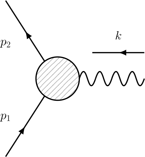
Figure 5: 3-pt amplitude. Figure reproduced from Ref. [103]

As we know from Sec. 4.3, it is possible to recast the spin structure of the amplitudes in Eq. (4.71) in an exponential form:

$$\langle 2^{b}1^{a}\rangle^{\odot 2s} =[2^{b}|^{\odot 2s}\!\exp\!\bigg{(}\!{-i}\frac{k_{\mu}\varepsilon_{\nu}^{+}\bar{\sigma}^{\mu\nu}}{p_{1}\cdot\varepsilon^{+}}\bigg{)}|1^{a}]^{\odot 2s}\,,$$ (4.72a)

$$[2^{b}1^{a}]^{\odot 2s} =\langle 2^{b}|^{\odot 2s}\!\exp\!\bigg{(}\!{-i}\frac{k_{\mu}\varepsilon_{\nu}^{-}\sigma^{\mu\nu}}{p_{1}\cdot\varepsilon^{-}}\bigg{)}|1^{a}\rangle^{\odot 2s}\,,$$ (4.72b)

where we have used as the algebraic realizations of $J^{\mu\nu}$ the tensor-product
$-(\sigma^{\mu\nu}\otimes{\hbox to0.0pt{1\hss}\hskip 1.6pt\hbox{1}}+{\hbox to0.0pt{1\hss}\hskip 1.6pt\hbox{1}}\otimes\ \sigma^{\mu\nu})\equiv-\sigma^{\mu\nu}$ for the chiral basis and $-(\bar{\sigma}^{\mu\nu}\otimes{\hbox to0.0pt{1\hss}\hskip 1.6pt\hbox{1}}+{\hbox to0.0pt{1\hss}\hskip 1.6pt\hbox{1}}\otimes\ \bar{\sigma}^{\mu\nu})\equiv-\bar{\sigma}^{\mu\nu}$ for the anti-chiral basis.

Note that a consistent picture of spin-induced multipoles of a pointlike particle must be formulated in the particle’s rest frame. However, the spin operator is defined in App. (B) for momentum $p_{\rm a}$, with $a=1,2$, but acts, in the rest frame, on the states with momenta $p_{\rm a}\pm k/2$. The cure for that is to take into account an additional Lorentz boost, needed to bridge the gap between two states with different momenta, Ref. [81].
To start, we note that any two four-vectors $p_{1}$ and $p_{2}$ of equal mass $m$ may be related by the spinorial transformations:

$$|2^{b}\rangle=U_{12~{}a}^{~{}~{}b}\exp\!\bigg{(}\frac{i}{m^{2}}p_{1}^{\mu}k^{\nu}\sigma_{\mu\nu}\!\bigg{)}|1^{a}\rangle,\qquad|2^{b}]=U_{12~{}a}^{~{}~{}b}\exp\!\bigg{(}\frac{i}{m^{2}}p_{1}^{\mu}k^{\nu}\bar{\sigma}_{\mu\nu}\!\bigg{)}|1^{a}],$$ (4.73)

where $U_{12}\text{in}SU(2)$ is a little-group transformation that depends on the specifics of the massive-spinor realization.
The self-duality property of the spinorial generators, $\sigma^{\mu\nu}=\frac{i}{2}\epsilon^{\mu\nu\rho\sigma}\sigma_{\rho\sigma}$, allow us to easily rewrite the above exponents as

$$\frac{i}{m^{2}}\,p_{1}^{\mu}k^{\nu}\sigma_{\mu\nu,\alpha}^{~{}~{}~{}~{}\;\beta}=k\cdot a_{\alpha}^{~{}\beta},\qquad\frac{i}{m^{2}}\,p_{1}^{\mu}k^{\nu}\bar{\sigma}^{~{}~{}~{}\dot{\alpha}}_{\mu\nu,~{}\dot{\beta}}=-k\cdot a^{\dot{\alpha}}_{~{}\,\dot{\beta}},$$ (4.74)

where we have defined chiral representations for the Pauli-Lubanski operators, Ref. [103],

$$a_{~{}~{}\alpha}^{\mu,~{}\,\beta}=\frac{1}{2m^{2}}\epsilon^{\mu\nu\rho\sigma}p_{a\,\nu}\sigma_{\rho\sigma,\alpha}^{~{}~{}~{}~{}\;\beta}\,,\qquad a^{\mu,\dot{\alpha}}_{~{}~{}~{}\,\dot{\beta}}=\frac{1}{2m^{2}}\epsilon^{\mu\nu\rho\sigma}p_{a\,\nu}\bar{\sigma}^{~{}~{}~{}\dot{\alpha}}_{\rho\sigma,~{}\dot{\beta}}.$$ (4.75)

Notice that, already at this level, we are free to pick $p_{\rm a}=p_{1}+k/2$ instead of $p_{1}$, as the product $k\cdot a$ remains the same.

The natural extension to higher-spin states of the Pauli-Lubanski operators in the chiral representations, is simply the analogous of Eq. (C.5):

$$(a^{\mu})_{\alpha_{1}\dots\alpha_{2s}}^{~{}~{}~{}~{}~{}~{}~{}~{}\beta_{1}\dots\beta_{2s}}=a_{~{}~{}\alpha_{1}}^{\mu,~{}~{}\beta_{1}}\delta_{\alpha_{2}}^{\beta_{2}}\!\dots\delta_{\alpha_{2s}}^{\beta_{2s}}+\ldots+\delta_{\alpha_{1}}^{\beta_{1}}\!\dots\delta_{\alpha_{2s-1}}^{\beta_{2s-1}}a_{~{}~{}\alpha_{2s}}^{\mu,~{}~{}~{}\beta_{2s}}\,.$$ (4.76)

Therefore, we have

$$|\mathbf{2}\rangle^{\odot 2s} =e^{k\cdot a}\big{\{}U_{12}|\mathbf{1}\rangle\big{\}}^{\!\odot 2s}\,,\qquad|\mathbf{2}]^{\odot 2s}\!=e^{-k\cdot a}\big{\{}U_{12}|\mathbf{1}]\big{\}}^{\!\odot 2s}\,,$$ (4.77)

$$\langle\mathbf{2}|^{\odot 2s} =\big{\{}U_{12}\langle\mathbf{1}|\big{\}}^{\!\odot 2s}e^{-k\cdot a}\,,\>\,\quad[\mathbf{2}|^{\odot 2s}\!=\big{\{}U_{12}[\mathbf{1}|\big{\}}^{\!\odot 2s}e^{k\cdot a}\,,$$

where the second line follows from the antisymmetry of $\sigma^{\mu\nu}$ and $\bar{\sigma}^{\mu\nu}$ in the sense of $\epsilon^{\alpha\beta}\sigma_{~{}~{}~{}\beta}^{\mu\nu,~{}\gamma}\epsilon_{\gamma\delta}=-\sigma_{~{}~{}~{}\delta}^{\mu\nu,~{}\alpha}$.

We are finally ready to inspect the spin dependence of the three-point amplitudes. Using Eq. (4.77), we can rewrite Eq. (4.71) as

$${\cal M}_{3}^{(s)}(k^{+}) =-\frac{\kappa}{2}\frac{x^{2}}{m^{2s-2}}[\mathbf{2}|^{\odot 2s}e^{-2k\cdot a}|\mathbf{1}]^{\odot 2s}\,,$$ (4.78a)

$${\cal M}_{3}^{(s)}(k^{-}) =-\frac{\kappa}{2}\frac{x^{-2}}{m^{2s-2}}\langle\mathbf{2}|^{\odot 2s}e^{2k\cdot a}|\mathbf{1}\rangle^{\odot 2s}\,.$$ (4.78b)

The apparent spin dependence in the amplitude formulae above is of the form $e^{\mp 2k\cdot a}$, while no such dependence seems to exist in the original formulae Eq. (4.71). Still, the true angular-momentum dependence inherent to the minimal-coupling amplitudes should not depend on the choice of the spinorial basis. This apparent contradiction is resolved by taking into account the transformations Eq. (4.73).
To fully grasp this statement, it is helpful to examine the following example: consider $\langle\mathbf{2}\mathbf{1}\rangle^{\odot 2s}$, in the chiral representation we have

$$\langle\mathbf{2}\mathbf{1}\rangle^{\odot 2s}=\big{\{}U_{12}\langle\mathbf{1}|\big{\}}^{\odot 2s}e^{-k\cdot a}|\mathbf{1}\rangle^{\odot 2s}\,,$$ (4.79)

whereas in the anti-chiral representation we have

$$\langle\mathbf{2}\mathbf{1}\rangle^{\odot 2s}=[\mathbf{2}|^{\odot 2s}e^{-2k\cdot a}|\mathbf{1}]^{\odot 2s}=\big{\{}U_{12}[\mathbf{1}|\big{\}}^{\odot 2s}e^{-k\cdot a}|\mathbf{1}]^{\odot 2s}\,.$$ (4.80)

We can now clearly see how in both cases we have the same spin dependence.

In light of these considerations, we strip the spin-states from the amplitudes in Eq. (4.78) to cleanly obtain the spin dependence (see App. (D)). Furthermore, as the the total angular momentum of a Kerr Black Hole is large, it is a good approximation to take the infinite-spin limit.
For example, if we were to consider once again $\langle\mathbf{2}\mathbf{1}\rangle^{\odot 2s}$ after this manipulation we would get:

$$\lim_{s\to\infty}m^{2s}(U_{12})^{\odot 2s}e^{-k\cdot a}.$$ (4.81)

Note that the factor of $m^{2s}$, that apparently diverges, cancels in the actual amplitudes. Thus

$${\cal M}_{3}^{(\infty)}(k^{+}) \approx-\frac{\kappa}{2}m^{2}x^{2}e^{-k\cdot a}\!\lim_{s\to\infty}(U_{12})^{\odot 2s},$$ (4.82a)

$${\cal M}_{3}^{(\infty)}(k^{-}) \approx-\frac{\kappa}{2}m^{2}x^{-2}e^{k\cdot a}\!\lim_{s\to\infty}(U_{12})^{\odot 2s}.$$ (4.82b)

The remaining unitary factor of $(U_{12})^{\odot 2s}$ parametrizes an arbitrary little-group transformation that corresponds to the choice of the spin quantization axis (see Ref. [103]). As such, it is inherently quantum-mechanical and therefore should be removed in the classical limit. Indeed, it also appears in the simple product of polarization tensors

$$\lim_{s\to\infty}\varepsilon_{2}\cdot\varepsilon_{1} =\lim_{s\to\infty}\frac{1}{m^{2s}}\langle\mathbf{2}\mathbf{1}\rangle^{\odot s}\odot[\mathbf{2}\mathbf{1}]^{\odot s}=$$ (4.83)

$$=\lim_{s\to\infty}\frac{1}{m^{2s}}\big{\{}U_{12}\langle\mathbf{1}|\big{\}}^{\!\odot s}e^{-k\cdot a}|\mathbf{1}\rangle^{\odot s}\big{\{}U_{12}[\mathbf{1}|\big{\}}^{\!\odot s}e^{k\cdot a}|\mathbf{1}]^{\odot s}=\lim_{s\to\infty}(U_{12})^{\odot 2s}\,.$$

So we can interpret the factor of $(U_{12})^{\odot 2s}$ as the state normalization in accord with the notion of GEV, and as such it cancels out whenever we compute a physical quantity.

5 Computing higher-point Amplitudes from the Soft Theorems

In this section, I will discuss how to use the soft theorems, in the spinor-helicity formalism, to obtain amplitudes with an increasing number of gravitons.
Soft theorems describe general properties of scattering amplitudes in the infrared (IR) regime where the four-momentum of one massless particle approaches zero, $p^{\mu}\rightarrow\epsilon p^{\mu}$ with $\epsilon\to 0$. In this limit it is possible to write down a recursion relation connecting the amplitude to a lower-point one with the soft particle removed. For soft gravitons with $h=\pm 2$ the recursions take the form

$$\mathcal{M}_{n+1}^{\pm 2}=\left(\frac{S^{(0)}_{\pm 2}}{\epsilon^{3}}+\frac{S^{(1)}_{\pm 2}}{\epsilon^{2}}+\frac{S^{(2)}_{\pm 2}}{\epsilon}\right)\mathcal{M}_{n}\,,$$ (5.1)

where $S^{(i)}_{\pm h}$ are called the soft factors. The soft factors are universal, in the sense that they do not depend on what other “hard” particles are involved in the scattering.
The soft graviton theorem was first formulated by Steven Weinberg in 1965 Ref. [104]. However, after some initial progress Ref. [105], Ref. [106], this approach saw little use for nearly twenty years.
A new life into the study of soft theorems was brought by the emergence of on-shell methods for calculating scattering processes. An important step in this development was made by Cachazo and Strominger Ref. [107]. Using the BCFW recursion relations Ref. [108], they were able to extend the graviton soft theorems up to sub-subleading order at tree level. Despite these rapid developments, all of the results derived with on-shell techniques were valid only for massless theories.
Recently, using the spinor-helicity formalism for massive particles introduced in Ref. [98] and discussed in Sec. 2, Falkowski and Machado established soft recursion relations valid for general theories with massive particles of any spin.

5.1 BCFW Recursion Relations

In this section I will discuss the BCFW recursion relations, Ref. [108]. Using these relations we depart from the traditional QFT workflow: the on-shell recursion relations allow us to compute amplitudes without making any reference to a Lagrangian or to Feynman diagrams.
Note that the ‘original’ BCFW relations apply exclusively to amplitudes involving only massless particles. In this section, I will focus solely on the massless case, while the massive case will be addressed in subsequent sections.

The idea behind the Britto-Cachazo-Feng-Witten (BCFW) recursion relations is to consider the amplitude $\mathcal{M}_{n}(p_{1},\dots,p_{n})$ as an analytic function of its complex momenta $p_{1},\dots,p_{n}$. The momenta are complexified by introducing a shift, which preserves on-shellness and momentum conservation, and which is linear in a complex variable $z$.

Let us shift one of the momenta, say $p_{j}^{\mu}$ with $j=1,\dots n$, by a vector $q^{\mu}$, i.e. 
$\hat{p}_{j}(z)=p_{j}+zq$, with $z\text{in}\mathbb{C}$. Furthermore, in order to preserve the total momentum conservation, let us shift another momentum $\hat{p}_{i}(z)=p_{i}-zq$. On-shellness requires that $\hat{p}^{2}_{j}(z)=\hat{p}^{2}_{i}(z)=0$, which in turn implies the orthogonality conditions $q^{2}=p_{j}\cdot q=p_{i}\cdot q=0$. The amplitude $\mathcal{M}_{n}(p_{1},\dots,p_{n})$ then becomes an analytic function $\mathcal{M}(z)$ of this shift parameter $z$.

It is a well known fact that unitarity, in the sense of the optical theorem, implies that the poles of an amplitude correspond to the exchange of on-shell intermediate states. This means that the original amplitude factorizes on its poles into two smaller amplitudes connected by a vanishing propagator. Diagrammatically,

where we have defined the momentum flowing through the propagator as

$$\hat{P}^{\mu}_{1,k}\equiv p_{1}^{\mu}+\dots+\hat{p}^{\mu}_{j}+\dots+p_{k}^{\mu}\,.$$ (5.2)

Notice that if $i$ and $j$ are on the same side of the diagram, $P_{1,k}^{\mu}$ is independent of $z$ and there is no pole.
Now, $\hat{P}_{1,k}^{2}=(P_{1,k}+zq)^{2}=P_{1,k}^{2}+2zP_{1,k}\cdot q$. The factorization poles occur when $\hat{P}_{1,k}(z)$ goes on-shell for some $z_{k}$, i.e. $0=\hat{P}_{1,k}^{2}=(P_{1,k}+z_{k}q)^{2}=P_{1,k}^{2}+2z_{k}P_{1,k}\cdot q$, therefore the poles are located at

$$z_{k}=-\frac{P^{2}_{1,k}}{2P_{1,k}\cdot q}\,,\qquad\mathrm{with}\quad z_{k}\neq 0\,.$$ (5.3)

Note that $\hat{P}^{2}_{1,k}(z)=2P_{1,k}\cdot q\,(z-z_{k})=-\dfrac{P^{2}_{1,k}}{z_{k}}(z-z_{k})$.
Now, $\mathcal{M}_{n}(z=0)$ corresponds to the original amplitude, which is analytic around the origin, as the poles occur at $z_{k}\neq 0$. Cauchy’s theorem states that on a contour $\mathcal{C}$ very close to the origin

$$\frac{1}{2\pi i}\oint_{\mathcal{C}}dz\frac{\mathcal{M}_{n}(z)}{z}=\mathop{\mathrm{Res}}_{z\rightarrow 0}\frac{\mathcal{M}_{n}(z)}{z}=\mathcal{M}_{n}(0)\,.$$ (5.4)

Furthermore, the global residue theorem states that over contour large enough to encompass all its poles,

$$\mathcal{M}_{n}(0)+\sum_{k}\mathop{\mathrm{Res}}_{z\rightarrow z_{k}}\frac{\mathcal{M}_{n}(z)}{z}=\mathop{\mathrm{Res}}_{z\rightarrow\infty}\frac{\mathcal{M}_{n}(z)}{z}\,,$$ (5.5)

where $z_{k}$ are the locations of the factorization poles.
If $\mathcal{M}_{n}(z)\rightarrow 0$ as $z\rightarrow\infty$, then the residue at infinity vanishes and we are left with

$$\mathcal{M}_{n}(0)+\sum_{k}\mathop{\mathrm{Res}}_{z\rightarrow z_{k}}\frac{\mathcal{M}_{n}(z)}{z}=0$$ (5.6)

Using then the factorization into two lower-point amplitudes connected by a vanishing propagator,

$$i\mathcal{M}_{n}(0) =-\sum_{k}\mathop{\mathrm{Res}}_{z\rightarrow z_{k}}\frac{i\mathcal{M}_{n}(z)}{z}\,=$$ (5.7)

$$=-\sum_{h=\pm}\sum_{k=2}^{n-2}\mathop{\mathrm{Res}}_{z\rightarrow z_{k}}\biggl{[}i\mathcal{M}_{k+1}(1,2,\dots,\hat{j},\dots,-\hat{P}^{-h}_{1,k})\frac{i}{z\hat{P}^{2}_{1,k}}\,i\mathcal{M}_{n-k+1}(\hat{P}_{1,k}^{h},k+1,\dots,\hat{i},\dots,n)\biggr{]}\,,$$

where $\mathcal{M}_{k+1}$ and $\mathcal{M}_{n-k+1}$ are the amplitudes on either side of the pole.
Recalling now that

$$\mathop{\mathrm{Res}}_{z\rightarrow z_{k}}\frac{\mathcal{M}_{n}(z)}{z}=\lim_{z\rightarrow z_{k}}(z-z_{k})\frac{\mathcal{M}_{n}(z)}{z}\,,\qquad\mathrm{and}\quad z-z_{k}=-\frac{z_{k}\hat{P}^{2}_{1,k}}{P^{2}_{1,k}}\,,$$ (5.8)

we finally obtain the BCFW recursion relations:

$$i\mathcal{M}(p_{1}\dots p_{n}) =$$ (5.9)

$$=\sum_{h=\pm}\sum_{k=2}^{n-2}\,\,i\mathcal{M}_{k+1}(1,\dots,\hat{j},\dots,-\hat{P}^{-h}_{1,k})\frac{i}{P^{2}_{1,k}}\,i\mathcal{M}_{n-k+1}(\hat{P}_{1,k}^{h},\dots,\hat{i},\dots,n)\,.$$

Notice that the sum is over the $(n-3)$ partitions of the $n$ momenta into two sets, with at least three momenta in both sets (even when considering complex momenta, the smallest possible on-shell amplitudes are the three-point ones).

To complete the proof of the on-shell recursion relations, it is necessary to show that $\mathcal{M}_{n}(z)\rightarrow 0$ as $z\rightarrow\infty$. This point is rather delicate, as for a generic amplitude, this behavior is not always assured; however, in the cases I will discuss, the residue at infinity will consistently be zero. A detailed discussion of all possible scenarios can be found in Ref. [109].

5.2 Soft Recursions

In this section, I will derive a formula that connects an $n+1$-point amplitude with at least one massless particle to an $n$-point amplitude. This formula captures the leading terms in the limit where the momentum of a massless particle is continuously taken to zero. This massless particle is referred to as soft, and the formula is referred to as the soft recursion. I will mainly follow Ref. [110] and Ref. [111].
I will employ a similar BCFW approach, but with generalizations to include massive particles. Additionally, the soft limits will be taken in a manifestly on-shell manner using an extra complex deformation of the external massless momenta.
In addition to the new soft theorems, the resulting master formula yields consistency conditions such as the conservation of electric charge, the Einstein equivalence principle, supergravity Ward identities, and the Weinberg-Witten theorem.

5.2.1 Momentum shift

As seen in Sec. 5.1, a crucial step for any amplitude to factorize is performing a shift of the complex momenta. I will now examine how to implement such a shift in the massive case and, as an additional step, deform the external massless momenta.
Consider a set of $n+1$ particles with momenta $p_{0}\dots p_{n}$ satisfying $\sum_{i=0}^{n}p_{i}=0$ and the on-shell conditions $p_{i}^{2}=m_{i}^{2}$. The particle labeled as $0$ is always massless, $p_{0}^{2}=0$, and it will be our soft particle. We perform a two-parameter deformation of this kinematics. One parameter $z$ controls complex deformation of the momenta of the particle $0$ and of two other particles, below labeled as $j$ and $k$. The other parameter $\epsilon$ controls the soft limit of the particle 0.
A convenient choice of the shifts is the following :

$$\hat{p}_{0}=\epsilon p_{0}-zq_{0}\,,\quad\hat{p}_{j}=p_{j}-\frac{(\epsilon-1)(p_{0}p_{k})-z(q_{0}p_{k})}{q_{j}p_{k}}q_{j}\,,\quad\hat{p}_{k}=p_{k}-\frac{(\epsilon-1)(p_{0}p_{j})-z(q_{0}p_{j})}{q_{k}p_{j}}q_{k}\,,$$ (5.10)

and the remaining particles remain un-shifted.
We now must fix the four-vectors $q_{0}$, $q_{j}$, $q_{k}$ in such a way that on-shellness and momentum conservation are preserved also on the shifted kinematics.
In order to preserve on-shellness, we impose

$$\begin{cases}\hat{p}_{0}^{2}=(\epsilon p_{0}-zq_{0})^{2}=0\\ \hat{p}_{j}=\biggl{(}p_{j}-\dfrac{(\epsilon-1)(p_{0}p_{k})-z(q_{0}p_{k})}{q_{j}p_{k}}q_{j}\biggr{)}^{2}=m_{j}^{2}\\ \hat{p}_{k}^{2}=p_{k}-\biggl{(}\dfrac{(\epsilon-1)(p_{0}p_{j})-z(q_{0}p_{j})}{q_{k}p_{j}}q_{k}\biggr{)}^{2}=m_{k}^{2}\end{cases}\rightarrow\begin{cases}p_{0}\cdot q_{0}=0\,,\,\,\,q_{0}^{2}=0\\ p_{j}\cdot q_{j}=0\,,\,\,\,q_{j}^{2}=0\\ p_{k}\cdot q_{k}=0\,,\,\,\,q_{k}^{2}=0\\ \end{cases}\,.$$ (5.11)

Furthermore, in order to preserve momentum conservation, we impose

$$\sum_{i=0}^{n}\hat{p}_{i} =\sum_{i=0}^{n}p_{i}+$$ (5.12)

$$\,+\biggl{[}(\epsilon-1)p_{0}-zq_{0}-\dfrac{(\epsilon-1)(p_{0}p_{k})-z(q_{0}p_{k})}{q_{j}p_{k}}q_{j}-\dfrac{(\epsilon-1)(p_{0}p_{j})-z(q_{0}p_{j})}{q_{k}p_{j}}q_{k}\biggr{]}=0\,,$$

thus the term in square bracket must vanish. Notice that as $\epsilon$ and $z$ are completely unrelated, in order for the second line of Eq. (5.12) to be null, each contribution must individually vanish, so

$$\begin{cases}p_{0}-\dfrac{p_{0}p_{k}}{q_{j}p_{k}}q_{j}-\dfrac{p_{0}p_{j}}{q_{k}p_{j}}q_{k}=0\\ q_{0}+\dfrac{q_{0}p_{k}}{q_{j}p_{k}}q_{j}+\dfrac{q_{0}p_{j}}{q_{k}p_{j}}q_{k}=0\end{cases}\,.$$ (5.13)

A possible solution for this system is simply obtained by squaring both equations

$$\begin{cases}\biggl{(}p_{0}-\dfrac{p_{0}p_{k}}{q_{j}p_{k}}q_{j}-\dfrac{p_{0}p_{j}}{q_{k}p_{j}}q_{k}\biggr{)}^{2}=0\\ \biggl{(}q_{0}+\dfrac{q_{0}p_{k}}{q_{j}p_{k}}q_{j}+\dfrac{q_{0}p_{j}}{q_{k}p_{j}}q_{k}\biggr{)}^{2}=0\end{cases}\Rightarrow\begin{cases}p_{0}\cdot q_{j}=0\,,\,\,\,p_{0}\cdot q_{k}=0\,,\,\,\,q_{j}\cdot q_{k}=0\\ q_{0}\cdot q_{j}=0\,,\,\,\,q_{0}\cdot q_{k}=0\,,\,\,\,q_{j}\cdot q_{k}=0\\ \end{cases}\,.$$ (5.14)

Altogether, the four-vectors $q_{0},q_{j},q_{k}$ satisfy

$$q_{0}^{2}=q_{j}^{2}=q_{k}^{2}=q_{0}p_{0}=q_{j}p_{j}=q_{k}p_{k}=0\,,\qquad q_{j}p_{0}=q_{k}p_{0}=q_{j}q_{0}=q_{k}q_{0}=q_{j}q_{k}=0\,.$$ (5.15)

5.2.2 Recursion

Consider an $n+1$ point amplitude $\mathcal{M}_{n+1}\equiv\mathcal{M}(1\dots n0)$. We denote $\hat{\mathcal{M}}^{z,\epsilon}_{n+1}$ its shifted version, which is $\mathcal{M}_{n+1}$ evaluated for the “hatted” kinematics in Eq. (5.10). Similarly, we denote $\mathcal{M}_{n}\equiv\mathcal{M}(1\dots n)$, and its shifted version by $\hat{\mathcal{M}}_{n}^{z,\epsilon}$.
Note that the trivial shift is $\hat{\mathcal{M}}^{0,1}=\mathcal{M}$.

At tree level $\hat{\mathcal{M}}^{z,\epsilon}$ is a meromorphic function of $z$, i.e. a function that is holomorphic on an open subset of the complex plane, except for a set of isolated points, which are poles of the function. Thus, all the singularities of $\hat{\mathcal{M}}^{z,\epsilon}$ are given by a finite set of simple poles at $z=z_{i}$. As in Sec. 5.1, we may now apply the Cauchy formula,

$$\hat{\mathcal{M}}^{0,\epsilon}_{n+1}=-\sum_{i}\mathop{\mathrm{Res}}_{z\to z_{i}}\dfrac{\hat{\mathcal{M}}^{z,\epsilon}_{n+1}}{z}+B_{\infty}\,,$$ (5.16)

where the boundary term $B_{\infty}$ is the residue at infinity. Once again, if $\hat{\mathcal{M}}^{z,\epsilon}_{n+1}$ goes to zero as $z\to\infty$ then $B_{\infty}=0$.
Assuming the residue at infinity to be null or at least finite in the limit $\epsilon\to 0$, the only poles of the integrand are at the solutions of

$$(\hat{p}_{0}(z)+p_{a_{1}}+\dots+p_{a_{m}})^{2}=0\,,$$ (5.17)

for any non-empty subset $\{a_{1},a_{2},\dots,a_{m}\}$ of $\{1,2,\dots,\dots,n\}$.
As seen in Sec. 5.1, the residue at each of these poles is determined by unitarity to be the product of two lower point amplitudes. For a pole at say $z=z_{m}$, the vector $\hat{P}_{0,m}-m^{2}_{0,m}=\hat{p}_{0}+p_{a_{1}}+\dots+p_{a_{m}}$ is null by construction, and the residue is given by

$$\hat{\mathcal{M}}^{0,\epsilon}_{n+1}=-\sum_{\mathcal{I}}\,\dfrac{\mathcal{M}_{m+1}(\hat{p}_{0},p_{a_{1}},\dots,p_{a_{m}},-\hat{P}_{0,m})\,\mathcal{M}_{n-m+1}(\hat{P}_{0,m},\overline{p_{a_{1}},\dots,p_{a_{m}}})}{P^{2}_{0,m}-m^{2}_{0,m}}\,,$$ (5.18)

where $\overline{a_{1},\dots,a_{m}}$ is the complement of $a_{1},\dots,a_{m}$, and we sum over all possible non-empty subsets $\mathcal{I}=\{a_{1},\dots,a_{m}\}$ of $\{1,\dots,n\}$.
Let us now separate the terms in the sum into two groups. The first group is those where the set $\mathcal{I}$ consists of a single element and the second group contains all other sets. The reason for this separation is that, as proven in Appendix A of Ref. [107], elements of the former becomes singular when $\lambda_{0}\to 0$ while elements of the latter remains finite.
In conclusion, we only focus on a subset of the poles related to the emission of the particle-0 from an external leg of the $n$-point amplitude $\mathcal{M}_{n}$, as $1/\epsilon^{m}$ terms in $\hat{\mathcal{M}}^{z,\epsilon}_{n+1}$ can only come from their residues.
There are $n$ such poles $z_{l}$ related to the solutions of the equations $\hat{P}_{0l}^{2}|_{z=z_{l}}=m_{l}^{2}$, where $\hat{P}_{0l}\equiv\hat{p}_{0}+\hat{p}_{l}$ and it is understood that $\hat{p}_{l}=p_{l}$ for $l\neq j,k$. The poles are located at:

$$0=\hat{P}_{0l}^{2}\big{|}_{z=z_{l}}-m_{l}^{2} =(\hat{p}_{0}+\hat{p}_{l})^{2}|_{z=z_{l}}-m_{l}^{2}=(\epsilon p_{0}-z_{l}q_{0}+\hat{p}_{l})^{2}-m_{l}^{2}\,=$$

$$=\epsilon^{2}p_{0}^{2}+z_{l}^{2}q_{0}^{2}+\hat{p}_{l}^{2}+2\epsilon p_{0}\cdot\hat{p}_{l}-2\epsilon z_{l}p_{0}\cdot q_{0}-2z_{l}q_{0}\cdot\hat{p}_{l}-m_{l}^{2}\,$$ (5.19)

using now on-shellness and Eq. (5.15), we find

$$z_{l}=\epsilon\frac{p_{0}p_{l}}{q_{0}p_{l}},\qquad l=1\dots n\,,$$ (5.20)

notice that this result holds true also for the shifted particles. Furthermore, we have $\hat{P}_{0l}^{2}-m_{l}^{2}=-2q_{0}p_{l}(z-z_{l})$, i.e. poles at $\hat{P}_{0l}^{2}\to m_{l}^{2}$ are in one-to-one correspondence with the poles at $z\to z_{l}$.

To sum up, we have:

$$\hat{\mathcal{M}}^{z,\epsilon}(1\dots n0)|_{\hat{P}_{0l}^{2}\to m_{l}^{2}}=-\frac{\hat{\mathcal{M}}^{z_{l},\epsilon}(1\dots P_{0l}\dots n)\hat{\mathcal{M}}^{z_{l},\epsilon}((-P_{0l})l0)}{\hat{P}_{0l}^{2}-m_{l}^{2}}\,=$$

$$\hskip 113.81102pt=\frac{\hat{\mathcal{M}}^{z_{l},\epsilon}(1\dots P_{0l}\dots n)\hat{\mathcal{M}}^{z_{l},\epsilon}((-P_{0l})l0)}{2q_{0}p_{l}(z-z_{l})}\,,$$ (5.21a)

$$\dfrac{\mathop{\mathrm{Res}}_{z\to z_{l}}\hat{\mathcal{M}}^{z,\epsilon}(0\dots n)}{z_{l}}=\frac{1}{\epsilon}\frac{\hat{\mathcal{M}}^{z_{l},\epsilon}(1\dots P_{0l}\dots n)\hat{\mathcal{M}}^{z_{l},\epsilon}((-P_{0l})l0)}{2p_{0}p_{l}}\,.$$ (5.21b)

Plugging this back into the Cauchy formula in Eq. (5.16) one obtains the soft recursion:

$$\hat{\mathcal{M}}^{0,\epsilon}(1\dots n0)=-\frac{1}{\epsilon}\sum_{l=1}^{n}\frac{\hat{\mathcal{M}}^{z_{l},\epsilon}(1\dots P_{0l}\dots n)\hat{\mathcal{M}}^{z_{l},\epsilon}((-P_{0l})l0)}{2p_{0}p_{l}}+\ \mathcal{O}(\epsilon^{0}).$$ (5.22)

As a final remark, notice that the boundary term in Eq. (5.16) is absorbed in $\mathcal{O}(\epsilon^{0})$, as it cannot produce singular terms in the $\epsilon\to 0$ limit.

5.2.3 Spinor shift

To compute the desired amplitudes, we find it convenient to use the spinor-helicity formalism. Accordingly, we will now focus on implementing the framework discussed in the previous sections at the spinorial level.

We begin by discussing spinor shifts that realize the momentum shift in Eq. (5.10). The discussion varies depending on whether the shifted particles $j$ and $k$ are massive or massless. In our case $m_{j}>0$ and $m_{k}>0$; the other possible cases are discusssed in Ref. [110].
One possible choice of the shift vectors $q$ in Eq. (5.10) is :

$$q_{0}\sigma=y\tilde{\lambda}_{0}\,,\qquad q_{j}\sigma=p_{j}\sigma\tilde{\lambda}_{0}\tilde{\lambda}_{0}\,,\qquad q_{k}\sigma=p_{k}\sigma\tilde{\lambda}_{0}\tilde{\lambda}_{0}\,,$$ (5.23)

where $y$ is an arbitrary spinor satisfying $\langle y0\rangle\neq 0$. It is easy to check that the constraints in Eq. (5.15) are satisfied by this choice.
We may now decompose also the shifted momenta into spinors:

$$\hat{p}_{0}\sigma=\lambda_{0}^{z}\tilde{\lambda}_{0}\,,\qquad\hat{p}_{j}\sigma=\chi_{j}^{J}\tilde{\chi}_{j\,J}^{z}\,,\qquad\hat{p}_{k}\sigma=\chi_{k}^{J}\tilde{\chi}_{k\,J}^{z}\,.$$ (5.24)

At the spinor level, a momentum shift can be achieved by shifting only the holomorphic (or anti-holomorphic) spinor while keeping the other spinor fixed.
In particular I will use the $\{0\bar{m}\bar{m}\}$ shift, defined as:

$${\rm\mathbf{\{}0\bar{m}\bar{m}\}}\mathrel{\mathop{\mathchar 58\relax}}\qquad\lambda_{0}^{z} =\epsilon\lambda_{0}-zy\,,$$

$$\tilde{\chi}_{j}^{z} =\tilde{\chi}_{j}+\frac{(\epsilon-1)\langle 0p_{k}0]-z\langle yp_{k}0]}{[0p_{j}p_{k}0]}[\mathbf{j}0]\tilde{\lambda}_{0}\,,$$ (5.25)

$$\tilde{\chi}_{k}^{z} =\tilde{\chi}_{k}-\frac{(\epsilon-1)\langle 0p_{j}0]-z\langle yp_{j}0]}{[0p_{j}p_{k}0]}[\mathbf{k}0]\tilde{\lambda}_{0}\,,$$

with all other spinors kept unshifted.

A crucial point that will become more relevant in the following sections, is that this shift is non-trivial for $z=\epsilon=0$: in this limit the spinors $\tilde{\chi}_{j/k}$ must shift to absorb the original momentum of the particle $0$. On the other hand, the shift is trivial for $z=0$ and $\epsilon=1$, but this is not the soft limit $\epsilon\to 0$.

For the remainder of this section, I will derive some identities that will be useful in later computations.
For the $\{0\bar{m}\bar{m}\}$ shift, the location of the poles in Eq. (5.20) can be recast as:

$$z_{l}=\epsilon\frac{\langle 0p_{l}0]}{\langle yp_{l}0]}\,;\qquad\text{which, for $m_{l}=0$, reduces to:}\quad z_{l}=\epsilon\frac{\langle 0l\rangle}{\langle yl\rangle}\,.$$ (5.26)

At the poles, the shifted spinors can be expressed as

$$\lambda_{0}^{z_{l}} =\epsilon\frac{\langle y0\rangle}{\langle yp_{l}0]}p_{l}\sigma\tilde{\lambda}_{0}\,,$$

$$\tilde{\chi}_{j}^{z_{l}} =\tilde{\chi}_{j}-\frac{2p_{0}p_{k}}{[0p_{j}p_{k}0]}[\mathbf{j}0]\tilde{\lambda}_{0}+\epsilon\frac{\langle y0\rangle[0p_{k}p_{l}0]}{\langle yp_{l}0][0p_{j}p_{k}0]}[\mathbf{j}0]\tilde{\lambda}_{0}\,$$ (5.27)

$$\tilde{\chi}_{k}^{z_{l}} =\tilde{\chi}_{k}+\frac{2p_{0}p_{j}}{[0p_{j}p_{k}0]}[\mathbf{k}0]\tilde{\lambda}_{0}-\epsilon\frac{\langle y0\rangle[0p_{j}p_{l}0]}{\langle yp_{l}0][0p_{j}p_{k}0]}[\mathbf{k}0]\tilde{\lambda}_{0}\,.$$

These identities allow us to rewrite $\hat{P}_{0l}$ at the poles as:

$$\text{for $l\neq j,k$}\quad\rightarrow\quad\hat{P}_{0l}\sigma|_{z_{l}}=\hat{p}_{0}\sigma|_{z_{l}}+p_{l}\sigma|_{z_{l}}=\lambda_{0}^{z_{l}}\tilde{\lambda}_{0}+p_{l}\sigma=\epsilon\frac{\langle y0\rangle}{\langle yp_{l}0]}p_{l}\sigma\tilde{\lambda}_{0}\tilde{\lambda}_{0}+p_{l}\sigma\,.$$ (5.28)

Furthermore, since $\hat{P}_{0l}|_{z=z_{l}}$ is on shell by definition, we may also factorize it into spinors:

$$l\neq j,k\,\mathrel{\mathop{\mathchar 58\relax}}\begin{cases}\hat{P}_{0l}\sigma|_{z_{l}}=\chi_{0l}^{L}\tilde{\chi}_{0l\,L},\quad\chi_{0l}=\chi_{l}\,,\quad\tilde{\chi}_{0l}=\tilde{\chi}_{l}+\epsilon\dfrac{\langle y0\rangle}{\langle yp_{l}0]}[\mathbf{l}0]\tilde{\lambda}_{0}\,,\quad\text{if}\,\,m_{l}>0\\ \hat{P}_{0l}\sigma|_{z_{l}}=\lambda_{0l}\tilde{\lambda}_{0l}\,,\quad\,\,\,\lambda_{0l}=\lambda_{l}\,,\quad\tilde{\lambda}_{0l}=\tilde{\lambda}_{l}+\epsilon\dfrac{\langle y0\rangle}{\langle yl\rangle}\tilde{\lambda}_{0}\,,\qquad\quad\,\text{if}\,\,m_{l}=0\end{cases}$$ (5.29)

Similarly at $z_{j}$ and $z_{k}$ we have the decomposition

$$\hat{P}_{0j}\sigma|_{z_{j}} =p_{j}\sigma-\frac{2p_{0}p_{k}}{[0p_{j}p_{k}0]}p_{j}\sigma\tilde{\lambda}_{0}\tilde{\lambda}_{0}\,\Rightarrow\,\chi_{0j}=\chi_{j}\,,\quad\tilde{\chi}_{0j}=\tilde{\chi}_{j}-\frac{2p_{0}p_{k}}{[0p_{j}p_{k}0]}[\mathbf{j}0]\tilde{\lambda}_{0}\,,$$ (5.30)

$$\hat{P}_{0k}\sigma|_{z_{k}} =p_{k}\sigma+\frac{2p_{0}p_{j}}{[0p_{j}p_{k}0]}p_{k}\sigma\tilde{\lambda}_{0}\tilde{\lambda}_{0}\,\Rightarrow\,\chi_{0k}=\chi_{k}\,,\quad\tilde{\chi}_{0k}=\tilde{\chi}_{k}+\frac{2p_{0}p_{j}}{[0p_{j}p_{k}0]}[\mathbf{k}0]\tilde{\lambda}_{0}\,.$$

Note that $\hat{P}_{0j}\sigma|_{z_{j}}$ and $\hat{P}_{0k}\sigma|_{z_{k}}$, and similarly the shifts $\tilde{\chi}_{j}^{z_{k}}$ and $\tilde{\chi}_{k}^{z_{j}}$, are independent of $\epsilon$.

5.3 Soft Theorems

We are now ready to apply the recursion formula in Eq. (5.22) to derive the soft factors for amplitudes involving particles of any mass and spin, with the graviton as the soft particle. I will restrict the analysis to the case of single soft particle emission.

Consider a gravity theory where the massless spin-2 graviton is minimally coupled to matter and to itself.
In the on-shell formalism, the minimal coupling of the graviton to two matter particle of same mass $m>0$ and spin $s$ corresponds to the on-shell 3-point amplitudes in Eq. (4.31):

$$\mathcal{M}(p_{1},-p_{2},k_{3}^{-})=-\frac{\kappa}{2}\frac{\langle 3p_{1}\zeta]^{2}}{[3\zeta]^{2}}\frac{[\mathbf{2}\mathbf{1}]^{2s}}{m^{2s}}\,,\qquad\mathcal{M}(p_{1},-p_{2},k_{3}^{+})=-\frac{\kappa}{2}\frac{\langle\zeta p_{1}3]^{2}}{[3\zeta]^{2}}\frac{\langle\mathbf{2}\mathbf{1}\rangle^{2s}}{m^{2s}}\,,$$ (5.31)

whereas the pure gravity on-shell 3-point amplitudes correspond to Eq. (4.18):

$$\mathcal{M}(k_{1}^{-},-k_{2}^{-},k_{3}^{+})=-\frac{\kappa}{2}\frac{\langle 12\rangle^{6}}{\langle 13\rangle^{2}\langle 23\rangle^{2}}\,,\qquad\mathcal{M}(k_{1}^{+},-k_{2}^{+},k_{3}^{-})=-\frac{\kappa}{2}\frac{[12]^{6}}{[13]^{2}[23]^{2}}\,.$$ (5.32)

Without loss of generality, we may focus on the emission of a soft graviton with plus-helicity . Thus, the shifted three-point amplitude computed at the $z_{l}$-poles is:

$$\hat{\mathcal{M}}^{z_{l},\epsilon}((-\hat{P}_{0l})l0^{+}_{h})=-\frac{\kappa}{2}\,\frac{\langle yp_{l}0]^{2}}{\epsilon^{2}\langle 0y\rangle^{2}}\,.$$ (5.33)

Plugging this back into Eq. (5.22) we obtain:

$$\hat{\mathcal{M}}^{0,\epsilon}(1\dots n0^{+}_{h})=\frac{\kappa}{2}\,\frac{1}{\epsilon^{3}}\sum_{l=1}^{n}\frac{\langle yp_{l}0]^{2}}{(2p_{0}p_{l})\langle 0y\rangle^{2}}\hat{\mathcal{M}}^{z_{l},\epsilon}(1\dots\hat{P}_{0l}\dots n)+\mathcal{O}(\epsilon^{0})\,.$$ (5.34)

To proceed we need to expand the $n$-point amplitude above in powers of $\epsilon$.
As shown in App. (E), we have

$$\hat{\mathcal{M}}^{z_{l},\epsilon}(1\dots\hat{P}_{0l}\dots n)=\left\{1+\epsilon\dfrac{\langle 0y\rangle}{\langle yp_{l}0]}\tilde{\mathcal{D}}_{l}+\frac{\epsilon^{2}}{2}\dfrac{\langle 0y\rangle^{2}}{\langle yp_{l}0]^{2}}\tilde{\mathcal{D}}_{l}^{2}\right\}\hat{\mathcal{M}}^{0,0}(1\dots n)+\mathcal{O}(\epsilon^{3})\,,$$ (5.35)

where the differential operator $\tilde{\cal D}_{l}$ is

$$\tilde{\mathcal{D}}_{l}=[0\mathbf{l}][0\partial_{l}]+\dfrac{[0p_{k}p_{l}0]}{[0p_{j}p_{k}0]}[0\mathbf{j}][0\partial_{j}]-\dfrac{[0p_{j}p_{l}0]}{[0p_{j}p_{k}0]}[0\mathbf{k}][0\partial_{k}]\,,\qquad{\rm for}\,\,l\neq j,k,$$ (5.36)

and $\tilde{\cal D}_{l}=0$ for $l=j,k$ .

Plugging the expanded $\hat{\mathcal{M}}^{z_{l},\epsilon}$ back into Eq. (5.34) we obtain the soft theorem in the standard form:

$$\hat{\mathcal{M}}^{0,\epsilon}(1\dots n0_{h}^{+})=\bigg{\{}\frac{1}{\epsilon^{3}}S_{+2}^{(0)}+\frac{1}{\epsilon^{2}}S_{+2}^{(1)}+\frac{1}{\epsilon}S_{+2}^{(0)}\bigg{\}}\hat{\mathcal{M}}^{0,0}(1\dots n)+\mathcal{O}(\epsilon^{0})\,,$$ (5.37)

where we have defined

$$S^{(0)}_{+2}=\frac{\kappa}{2}\sum_{l=1}^{n}\dfrac{\langle yp_{l}0]^{2}}{(2p_{0}\cdot p_{l})\langle 0y\rangle^{2}},\quad S^{(1)}_{+2}=\frac{\kappa}{2}\sum_{l=1}^{n}\dfrac{\langle yp_{l}0]}{(2p_{0}\cdot p_{l})\langle 0y\rangle}\tilde{\mathcal{D}}_{l},\quad S^{(2)}_{+2}=\frac{\kappa}{4}\sum_{l=1}^{n}\frac{1}{4p_{0}\cdot p_{l}}\tilde{\mathcal{D}}_{l}\tilde{\mathcal{D}}_{l}\,.$$ (5.38)

It is important to remark that the soft factors do not depend on $y$ (either as a consequence of momentum conservation or of angular momentum conservation), see Ref. [110].
The soft factors above are the natural extension to the massive case of the ones presented in Ref. [107] and Ref. [111], moreover $S^{(0)}_{+2}$ is nothing but the Weinberg soft factor.

Finally, notice that for the emission of a minus-helicity graviton the computation is the same, and the final result is related to the former by a parity transformation, see Ref. [110].

5.3.1 Soft exponentiation

I now discuss the exponential representation of the soft theorems.
Ref. [112] showed that the soft theorem for gravitons and gluons could be written in terms of an exponential operator acting on lower point amplitudes. Furthermore, in Ref. [110], it was shown that the exponential operator can be extended for amplitudes with massive particles of any spin and with a soft particle of any integer helicity $|h|\leq 2$.

The Taylor expansion in Eq. (5.35) has been trucated at second order, nonetheless we may consider the complete series. It is straightforward to check that it can be recast in the exponential form:

$$\hat{\mathcal{M}}^{z_{l},\epsilon}(1\dots\hat{P}_{0l}\dots n)=\exp\left(\epsilon\frac{\langle 0y\rangle}{\langle yp_{l}0]}\tilde{\mathcal{D}}_{l}\right)\hat{\mathcal{M}}^{0,0}(1\dots n)+\mathcal{O}(\epsilon^{3}).$$ (5.39)

Substituting now in Eq. (5.37), we obtain:

$$\hat{\mathcal{M}}^{0,\epsilon}(1\dots n0^{+}_{h}) =\frac{\kappa}{2}\,\frac{1}{\epsilon^{3}}\sum_{l=1}^{n}\frac{\langle yp_{l}0]^{2}}{(2p_{0}p_{l})\langle 0y\rangle^{2}}\hat{\mathcal{M}}^{z_{l},\epsilon}(1\dots\hat{P}_{0l}\dots n)+\mathcal{O}(\epsilon^{0})=$$

$$=\frac{\kappa}{2}\,\frac{1}{\epsilon^{3}}\sum_{l=1}^{n}\frac{\langle yp_{l}0]^{2}}{(2p_{0}p_{l})\langle 0y\rangle^{2}}\exp\left(\epsilon\frac{\langle 0y\rangle}{\langle yp_{l}0]}\tilde{\mathcal{D}}_{l}\right)\hat{\mathcal{M}}^{0,0}(1\dots n)+\mathcal{O}(\epsilon^{0})\,,$$ (5.40)

where the differential operator $\tilde{\mathcal{D}}_{l}$ is given in Eq. (5.36).

5.3.2 Consistency checks

I conclude this discussion on the soft theorems by verifying that the formulae derived in the previous sections using the spinor-helicity formalism are consistent with those found in the literature, which were obtained through different approaches.

As seen in Ref. [110], the Taylor expansion around $\epsilon\to 0$ of the minimally coupled gravity amplitude in the soft limit can be recast in an exponential form Eq. (5.3.1):

$$\hat{\mathcal{M}}^{0,\epsilon}(1\dots n0^{+}_{h}) =\frac{\kappa}{2}\,\frac{1}{\epsilon^{3}}\sum_{l=1}^{n}\frac{\langle yp_{l}0]^{2}}{(2p_{0}p_{l})\langle 0y\rangle^{2}}\exp\left(\epsilon\frac{\langle 0y\rangle}{\langle yp_{l}0]}\tilde{\mathcal{D}}_{l}\right)\hat{\mathcal{M}}^{0,0}(1\dots n)+\mathcal{O}(\epsilon^{0})=$$

$$=\frac{\kappa}{2}\,\frac{1}{\epsilon^{3}}\sum_{l=1}^{n}\frac{\langle yp_{l}0]^{2}}{(2p_{0}p_{l})\langle 0y\rangle^{2}}\exp\Biggl{\{}\epsilon\frac{\langle 0y\rangle}{\langle yp_{l}0]}\,\times$$ (5.41)

$$\times\left([0\mathbf{l}][0\partial_{l}]+\dfrac{[0p_{k}p_{l}0]}{[0p_{j}p_{k}0]}[0\mathbf{j}][0\partial_{j}]-\dfrac{[0p_{j}p_{l}0]}{[0p_{j}p_{k}0]}[0\mathbf{k}][0\partial_{k}]\right)\Biggr{\}}\hat{\mathcal{M}}^{0,0}(1\dots n)+\mathcal{O}(\epsilon^{0})\,.$$

We are now interested in comparing this result with the one originally obtained by Cachazo and Strominger in Ref. [107] and analyzed comprehensively by Guevara et all in Ref. [100]:

$${\cal M}_{n+1}=\frac{\kappa}{2}\sum_{i=1}^{n}\left[\frac{(p_{i}\cdot\varepsilon)^{2}}{p_{i}\cdot k}+i\frac{(p_{i}\cdot\varepsilon)(k_{\mu}\varepsilon_{\nu}J_{i}^{\mu\nu})}{p_{i}\cdot k}-\frac{1}{2}\frac{(k_{\mu}\varepsilon_{\nu}J_{i}^{\mu\nu})^{2}}{p_{i}\cdot k}\right]{\cal M}_{n}+{\cal O}(k^{2})\,.$$ (5.42)

Here the soft momentum $k$ corresponds to the external soft graviton, and we have constructed its polarization tensor as $\varepsilon_{\mu\nu}=\varepsilon_{\mu}\varepsilon_{\nu}$.
In Ref. [100] it was shown that for the three- and four- point amplitudes we are able to recast the term in square bracket in an exponential form. Following this intuition, we may write

$${\cal M}_{n+1}(1\dots n,0^{+})=\frac{\kappa}{2}\sum_{i=1}^{n}\frac{\left(p_{i}\cdot\varepsilon\right)^{2}}{p_{i}\cdot k}\exp\left(i\frac{k_{\mu}\varepsilon_{\nu}J^{\mu\nu}_{i}}{p_{i}\cdot\varepsilon}\right){\cal M}_{n}(1\dots n)\,.$$ (5.43)

We now recall that $\hat{\cal M}=\hat{\cal M}^{(0,1)}$. Thus, to make contact with Eq. (5.3.2) we generalize to the case of arbitrary $\epsilon$ shift. To this end, we perform the $\{0,\bar{m},\bar{m}\}$ shift in Eq. (5.2.3), where we choose once again the shifted spinors to be the one associated with the soft graviton “0”, and the massive spinors j, k, and expand around $\epsilon\rightarrow 0$:

$$\mathcal{M}^{(0,\epsilon)}_{n}(1\dots n)=\mathcal{M}^{(0,\epsilon)}_{n}(1\dots\hat{\mathbf{j}}\dots\hat{\mathbf{k}}\dots n)\,,\qquad\mathcal{M}^{(0,\epsilon)}_{n}=\sum_{m=0}^{\infty}\dfrac{\epsilon^{m}}{m!}\bigg{(}\frac{\partial}{\partial\epsilon}\bigg{)}^{\!\!m}\mathcal{M}^{(0,\epsilon)}_{n}\Big{|}_{\epsilon=0}\,,$$ (5.44)

$$\frac{\partial}{\partial\epsilon}\mathcal{M}_{n}^{(0,\epsilon)}=\left(\frac{\partial\tilde{\chi}_{j}}{\partial\epsilon}\frac{\partial}{\partial\tilde{\chi}_{j}}+\frac{\partial\tilde{\chi}_{k}}{\partial\epsilon}\frac{\partial}{\partial\tilde{\chi}_{k}}\right)\mathcal{M}_{n}^{(0,\epsilon)}=$$

$$\qquad\qquad=\left(\frac{\langle 0y\rangle[0p_{k}p_{l}0]}{\langle yp_{l}0][0p_{j}p_{k}0]}[0\mathbf{j}][0\frac{\partial}{\partial\tilde{\chi}_{j}}]-\frac{\langle 0y\rangle[0p_{j}p_{l}0]}{\langle yp_{l}0][0p_{j}p_{k}0]}[0\mathbf{k}][0\frac{\partial}{\partial\tilde{\chi}_{k}}]\right)\mathcal{M}_{n}^{(0,\epsilon)}\,.$$ (5.45)

Altogether

$$\mathcal{M}_{n+1}^{(0,\epsilon)}(1\dots n,0^{+})=\frac{\kappa}{2}\sum_{i=1}^{n}\frac{1}{\epsilon^{3}}\frac{\left(p_{i}\cdot\varepsilon\right)^{2}}{p_{i}\cdot k}\exp\left(i\frac{k_{\mu}\varepsilon_{\nu}J^{\mu\nu}_{i}}{p_{i}\cdot\varepsilon}\right)\left(\sum_{m=0}^{\infty}\dfrac{\epsilon^{m}}{m!}\bigg{(}\frac{\partial}{\partial\epsilon}\bigg{)}^{\!\!m}\mathcal{M}^{(0,\epsilon)}_{n}\Big{|}_{\epsilon=0}\right)=$$

$$\qquad=\frac{\kappa}{2}\sum_{i=1}^{n}\frac{1}{\epsilon^{3}}\frac{\left(p_{i}\cdot\varepsilon\right)^{2}}{p_{i}\cdot k}\exp\left(i\frac{k_{\mu}\varepsilon_{\nu}J^{\mu\nu}_{i}}{p_{i}\cdot\varepsilon}\right)\,\times$$

$$\qquad\quad\times\left(\sum_{m=0}^{\infty}\dfrac{\epsilon^{m}}{m!}\left(\frac{\langle 0y\rangle[0p_{k}p_{l}0]}{\langle yp_{l}0][0p_{j}p_{k}0]}[0\mathbf{j}][0\frac{\partial}{\partial\tilde{\chi}_{j}}]-\frac{\langle 0y\rangle[0p_{j}p_{l}0]}{\langle yp_{l}0][0p_{j}p_{k}0]}[0\mathbf{k}][0\frac{\partial}{\partial\tilde{\chi}_{k}}]\right)^{\!\!m}\mathcal{M}^{(0,\epsilon)}_{n}\Big{|}_{\epsilon=0}\right)=$$

$$\qquad=\frac{\kappa}{2}\sum_{i=1}^{n}\frac{1}{\epsilon^{3}}\frac{\left(p_{i}\cdot\varepsilon\right)^{2}}{p_{i}\cdot k}\exp\left(\epsilon\frac{\langle 0y\rangle}{\langle yp_{l}0]}[0\mathbf{l}][0\frac{\partial}{\partial\tilde{\chi}_{l}}]\right)\,\times$$

$$\qquad\quad\times\exp\left(\frac{\langle 0y\rangle[0p_{k}p_{l}0]}{\langle yp_{l}0][0p_{j}p_{k}0]}[0\mathbf{j}][0\frac{\partial}{\partial\tilde{\chi}_{j}}]-\frac{\langle 0y\rangle[0p_{j}p_{l}0]}{\langle yp_{l}0][0p_{j}p_{k}0]}[0\mathbf{k}][0\frac{\partial}{\partial\tilde{\chi}_{k}}]\right)\mathcal{M}^{(0,\epsilon)}_{n}\Big{|}_{\epsilon=0}=$$

$$\qquad=\frac{\kappa}{2}\sum_{i=1}^{n}\frac{1}{\epsilon^{3}}\frac{\left(p_{i}\cdot\varepsilon\right)^{2}}{p_{i}\cdot k}\exp\left(\epsilon\frac{\langle 0y\rangle}{\langle yp_{l}0]}\tilde{\mathcal{D}}_{l}\right)\mathcal{M}^{(0,0)}_{n}\,,$$ (5.46)

where we have used the parity reversed form of Eq. (4.55) to go from the second to the third line.
From Eq. (5.3.2) it is clear that the two formulas match perfectly, confirming the consistency of our procedure. Moreover, by recalling that the soft expansion was performed by defining the parameter $\epsilon$ via the rescaling $p^{\mu}=\epsilon p^{\mu}$, or in spinor variables $\lambda_{0}=\epsilon\lambda_{0}$, we can fully absorb the $\epsilon$ in this formula. As a result, the two outcomes are exactly the same, further validating our consistency check.

6 Gravitational Compton Amplitude from the Soft Theorems

In this section I will apply the soft theorems discussed in Sec. 5 to the three-point amplitudes obtained in Sec. 4 to obtain the four-point Compton gravitational amplitude.
As seen in Sec. 5.3.2, our soft theorems can be formulated using Eq. (5.3.2) or Eq. (5.43) equivalently. In this section, I will use the latter formulation as most of the results found in literature are expressed in this way. Furthermore as I’m not interested in this section to explore the soft limit of the four-point amplitude, but rather to use the soft theorems to obtain this higher-point amplitude, I find it more convenient to use directly Eq. (5.43), rather than computing Eq. (5.3.2) and taking the $\epsilon\to 1$ limit.
I will start by discussing the spinless Schwarzschild case and later generalize also to the spinning Kerr case.

6.1 Compton Amplitude for Schwarzschild Black Holes

Our starting point are the three-point amplitudes Eq. (4.69), that I rewrite below for convenience,

$${\cal M}_{3}^{(s)}(p_{1},p_{2},k^{+}_{3})=\frac{\kappa}{2}\frac{\langle\mathbf{1}\mathbf{2}\rangle^{2s}x_{3}^{2}}{m^{2s-2}},\qquad\quad{\cal M}_{3}^{(s)}(p_{1},p_{2},k^{-}_{3})=\frac{\kappa}{2}\frac{[\mathbf{1}\mathbf{2}]^{2s}x_{3}^{-2}}{m^{2s-2}}\,.$$ (6.1)

As I’m now interested the Schwarzscild case, $s=0$; hence, after expliciting the $x$-factors, these amplitudes reduce to:

$${\cal M}_{3}^{(0)}(p_{1},p_{2},k^{+}_{3})=\kappa(p_{1}\cdot\varepsilon_{3}^{+})^{2}\,,\qquad\quad{\cal M}_{3}^{(0)}(p_{1},p_{2},k^{-}_{3})=\kappa(p_{1}\cdot\varepsilon_{3}^{-})^{2}\,.$$ (6.2)

Let us start by considering the plus-helicity case.
To get the corresponding four-point amplitude we may now use Eq. (5.43):

$${\cal M}_{4}^{(0)}(p_{1},p_{2},k_{3}^{+},k_{4}^{+})=\frac{\kappa}{2}\sum_{i=1}^{3}\frac{\left(p_{i}\cdot\varepsilon_{4}^{+}\right)^{2}}{p_{i}\cdot k_{4}}\exp\left(i\frac{k_{4,\mu}\varepsilon_{4,\nu}^{+}J^{\mu\nu}_{i}}{p_{i}\cdot\varepsilon_{4}^{+}}\right){\cal M}_{3}^{(0)}(p_{1},p_{2},k_{3}^{+})\,.$$ (6.3)

This result is gauge-independent, therefore we can make a convenient gauge choice to simplify the computations. Nonetheless, to make the final result general, we must express it too in a gauge-independent way.
A convenient gauge choice is the one in which we fix the reference vectors for the massless particles labeled $3$ and $4$ to be $\varepsilon_{3}=\varepsilon(3,4)$, $\varepsilon_{4}=\varepsilon(4,3)$, this way all products $p_{i}\cdot\varepsilon_{j}=0$, for $i,j=3,4$, and the sum in Eq. (6.3) reduces to:

$${\cal M}_{4}^{(0)}(p_{1},p_{2},k_{3}^{+},k_{4}^{+})=$$ (6.4)

$$\qquad=\frac{\kappa}{2}\left[\frac{\left(p_{1}\cdot\varepsilon_{4}^{+}\right)^{2}}{p_{1}\cdot k_{4}}\exp\left(i\frac{k_{4,\mu}\varepsilon_{4,\nu}^{+}J^{\mu\nu}_{1}}{p_{1}\cdot\varepsilon_{4}^{+}}\right)+\frac{\left(p_{2}\cdot\varepsilon_{4}^{+}\right)^{2}}{p_{2}\cdot k_{4}}\exp\left(i\frac{k_{4,\mu}\varepsilon_{4,\nu}^{+}J^{\mu\nu}_{2}}{p_{2}\cdot\varepsilon_{4}^{+}}\right)\right]{\cal M}_{3}^{(0)}(p_{1},p_{2},k_{3}^{+})\,.$$

Notice now that, as we are studying the scalar case, whenever the arguments of the exponential operators in Eq. (6.4) act on the three-point scalar amplitudes $\mathcal{M}_{3}^{(0)}$ they vanish. Thus:

$${\cal M}_{4}^{(0)}(p_{1},p_{2},k_{3}^{+},k_{4}^{+}) =\frac{\kappa}{2}\left[\frac{\left(p_{1}\cdot\varepsilon_{4}^{+}\right)^{2}}{p_{1}\cdot k_{4}}+\frac{\left(p_{2}\cdot\varepsilon_{4}^{+}\right)^{2}}{p_{2}\cdot k_{4}}\right]{\cal M}_{3}^{(0)}(p_{1},p_{2},k_{3}^{+})=$$

$$=\left(\dfrac{\kappa}{2}\right)^{\!2}\left[\frac{\left(p_{1}\cdot\varepsilon_{4}^{+}\right)^{2}}{p_{1}\cdot k_{4}}+\frac{\left(p_{2}\cdot\varepsilon_{4}^{+}\right)^{2}}{p_{2}\cdot k_{4}}\right]2(p_{1}\cdot\varepsilon_{3}^{+})^{2}\,.$$ (6.5)

Furthermore, from the three-point amplitude, we inherit the relation $p_{1}\cdot k_{3}=0$ . Using total momentum conservation, and the relations previously discussed we are able to rewrite Eq. (6.1) as:

$${\cal M}_{4}^{(0)}(p_{1},p_{2},k_{3}^{+},k_{4}^{+}) =\left(\dfrac{\kappa}{2}\right)^{\!2}\left[\frac{\left(p_{1}\cdot\varepsilon_{4}^{+}\right)^{2}}{p_{1}\cdot k_{4}}+\frac{\left((p_{1}+k_{3}+k_{4})\cdot\varepsilon_{4}^{+}\right)^{2}}{p_{2}\cdot k_{4}}\right]2(p_{1}\cdot\varepsilon_{3}^{+})^{2}=$$

$$=\dfrac{\kappa^{2}}{2}\left(p_{1}\cdot\varepsilon_{3}^{+}\right)^{2}\left(p_{1}\cdot\varepsilon_{4}^{+}\right)^{2}\left[\dfrac{1}{p_{1}\cdot k_{4}}+\dfrac{1}{p_{2}\cdot k_{4}}\right]=$$ (6.6)

$$=-\dfrac{\kappa^{2}}{2}\dfrac{\left(p_{1}\cdot\varepsilon_{3}^{+}\right)^{2}\left(p_{1}\cdot\varepsilon_{4}^{+}\right)^{2}(k_{3}\cdot k_{4})^{2}}{(p_{1}\cdot k_{4})(p_{2}\cdot k_{4})(k_{3}\cdot k_{4})}\,.$$

We remark that this expression is still gauge-invariant, and it is possible to rewrite it in a manifestly gauge invariant way if we notice that :

$$p_{1}\cdot F_{3}\cdot F_{4}\cdot p_{1}=-\left(p_{1}\cdot\varepsilon_{3}^{+}\right)\left(p_{1}\cdot\varepsilon_{4}^{+}\right)(k_{3}\cdot k_{4})\,,$$ (6.7)

where $F_{\mu\nu}$ is the field strength $F_{\mu\nu}=k_{\mu}\varepsilon_{\nu}-k_{\nu}\varepsilon_{\mu}$. Therefore,

$${\cal M}_{4}^{(0)}(p_{1},p_{2},k_{3}^{+},k_{4}^{+})=\dfrac{-\kappa^{2}\omega_{(0)}^{2}}{(2p_{1}\cdot k_{4})(2p_{2}\cdot k_{4})(2k_{3}\cdot k_{4})}\,,$$ (6.8)

where we have defined the quantity $\omega_{(0)}\equiv-2\,p_{1}\cdot F_{3}\cdot F_{4}\cdot p_{1}$.

The computation for the minus-helicity case is exactly the same, the only difference being the helicity of graviton-$3$ in $\omega_{(0)}$.
The remaining helicity configurations, i.e. when the graviton-$4$ has negative helicity, are easily obtained from Eq. (6.8) using parity and charge conjugation transformations.

This result is in perfect agreement with the ones found in the literature, e.g. see Ref. [81], Ref. [113].

6.2 Compton Amplitude for Kerr Black Holes

In this section I generalize the discussion in Sec. 6.1 to the case of spinning black holes.
Once again our starting point are the amplitudes

$${\cal M}_{3}^{(s)}(p_{1},p_{2},k^{+}_{3})=\frac{\kappa}{2}\frac{\langle\mathbf{1}\mathbf{2}\rangle^{2s}x_{3}^{2}}{m^{2s-2}},\qquad\quad{\cal M}_{3}^{(s)}(p_{1},p_{2},k^{-}_{3})=\frac{\kappa}{2}\frac{[\mathbf{1}\mathbf{2}]^{2s}x_{3}^{-2}}{m^{2s-2}}\,.$$ (6.9)

In this form the angular momentum dependence of the amplitude is hidden inside the spinors, however it is convenient to make it manifest:

$${\cal M}_{3}^{(s)}(p_{1},p_{2},k^{+}_{3}) =\dfrac{\kappa}{m^{2s}}(p_{1}\cdot\varepsilon_{3}^{+})^{2}[\mathbf{1}|^{2s}\exp\left(i\dfrac{k_{3,\mu}\varepsilon_{3,\nu}^{+}J_{1}^{\mu\nu}}{p_{1}\cdot\varepsilon_{3}^{+}}\right)|\mathbf{2}]^{2s}\,,$$ (6.10a)

$${\cal M}_{3}^{(s)}(p_{1},p_{2},k^{-}_{3}) =\dfrac{\kappa}{m^{2s}}(p_{1}\cdot\varepsilon_{3}^{-})^{2}\langle\mathbf{1}|^{2s}\exp\left(i\dfrac{k_{3,\mu}\varepsilon_{3,\nu}^{-}J_{1}^{\mu\nu}}{p_{1}\cdot\varepsilon_{3}^{-}}\right)|\mathbf{2}\rangle^{2s}\,,$$ (6.10b)

where I have used the fact that the action of the operator: $\exp\left(i\frac{k_{3,\mu}\varepsilon_{3,\nu}^{+}J^{\mu\nu}}{p_{1}\cdot\varepsilon_{3}^{+}}\right)$, on either the spinors $\langle\mathbf{1}|^{2s}$ ($[\mathbf{1}|^{2s}$) or $|\mathbf{2}\rangle^{2s}$ ($|\mathbf{2}]^{2s}$) gives the same result, to pick without loss of generality $J\to J_{1}$ .

Let us start by considering the plus-helicity case.
To get the corresponding four-point amplitude we may use once again Eq. (5.43):

$${\cal M}_{4}^{(s)}(p_{1},p_{2},k_{3}^{+},k_{4}^{+})=\frac{\kappa}{2}\sum_{i=1}^{3}\frac{\left(p_{i}\cdot\varepsilon_{4}^{+}\right)^{2}}{p_{i}\cdot k_{4}}\exp\left(i\frac{k_{4,\mu}\varepsilon_{4,\nu}^{+}J^{\mu\nu}_{i}}{p_{i}\cdot\varepsilon_{4}^{+}}\right){\cal M}_{3}^{(s)}(p_{1},p_{2},k_{3}^{+})\,.$$ (6.11)

Also this time, it is convenient to pick $\varepsilon_{3}=\varepsilon(3,4)$ and $\varepsilon_{4}=\varepsilon(4,3)$, this way all products $p_{i}\cdot\varepsilon_{j}=0$, for $i,j=3,4$ and the last term of the sum drops out. Hence,

$${\cal M}_{4}^{(s)}(p_{1},p_{2},k_{3}^{+},k_{4}^{+})=$$ (6.12)

$$\qquad=\frac{\kappa}{2}\left[\frac{\left(p_{1}\cdot\varepsilon_{4}^{+}\right)^{2}}{p_{1}\cdot k_{4}}\exp\left(i\frac{k_{4,\mu}\varepsilon_{4,\nu}^{+}J^{\mu\nu}_{1}}{p_{1}\cdot\varepsilon_{4}^{+}}\right)+\frac{\left(p_{2}\cdot\varepsilon_{4}^{+}\right)^{2}}{p_{2}\cdot k_{4}}\exp\left(i\frac{k_{4,\mu}\varepsilon_{4,\nu}^{+}J^{\mu\nu}_{2}}{p_{2}\cdot\varepsilon_{4}^{+}}\right)\right]{\cal M}_{3}^{(s)}(p_{1},p_{2},k_{3}^{+})\,.$$

Recalling now that the action of the operator $\exp\left(i\frac{k_{4,\mu}\varepsilon_{4,\nu}^{+}J^{\mu\nu}}{p_{1}\cdot\varepsilon_{4}^{+}}\right)$ gives the same result whether it acts on the spinors-$1$ or -$2$, the two exponential operators in Eq. (6.12) are completely equivalent and we can write:

$${\cal M}_{4}^{(s)}(p_{1},p_{2},k_{3}^{+},k_{4}^{+}) =\frac{\kappa}{2}\left[\frac{\left(p_{1}\cdot\varepsilon_{4}^{+}\right)^{2}}{p_{1}\cdot k_{4}}+\frac{\left(p_{2}\cdot\varepsilon_{4}^{+}\right)^{2}}{p_{2}\cdot k_{4}}\right]\exp\left(i\frac{k_{4,\mu}\varepsilon_{4,\nu}^{+}J_{1}^{\mu\nu}}{p_{1}\cdot\varepsilon_{4}^{+}}\right){\cal M}_{3}^{(s)}(p_{1},p_{2},k_{3}^{+})=$$

$$=\left(\dfrac{\kappa}{2}\right)^{\!2}\left[\frac{\left(p_{1}\cdot\varepsilon_{4}^{+}\right)^{2}}{p_{1}\cdot k_{4}}+\frac{\left(p_{2}\cdot\varepsilon_{4}^{+}\right)^{2}}{p_{2}\cdot k_{4}}\right]2(p_{1}\cdot\varepsilon_{3}^{+})^{2}\,\times$$ (6.13)

$$\times\dfrac{1}{m^{2s}}[\mathbf{1}|^{2s}\exp\left(i\frac{k_{4,\mu}\varepsilon_{4,\nu}^{+}J_{1}^{\mu\nu}}{p_{1}\cdot\varepsilon_{4}^{+}}\right)\exp\left(i\dfrac{k_{3,\mu}\varepsilon_{3,\nu}^{+}J_{1}^{\mu\nu}}{p_{1}\cdot\varepsilon_{3}^{+}}\right)|\mathbf{2}]^{2s}\,.$$

Notice that the first line of Eq. (6.2) is simply Eq. (6.1). This is to be expected, as the scalar contribution relative to the scattering of Kerr Black Holes is simply the Schwarzschild Compton scattering.

Focus now on the the second line. I define the operators:

$$J_{3}\equiv i\dfrac{k_{3,\mu}\varepsilon_{3,\nu}^{+}J_{1}^{\mu\nu}}{p_{1}\cdot\varepsilon_{3}^{+}}\,,\qquad\qquad J_{4}\equiv i\dfrac{k_{4,\mu}\varepsilon_{4,\nu}^{+}J_{1}^{\mu\nu}}{p_{1}\cdot\varepsilon_{4}^{+}}\,.$$ (6.14)

In general these operators do not commute, therefore the product of the two exponentials is not just the exponential of the sum. Nonetheless using the Baker-Campbell-Hausdorf formula:

$$e^{X}e^{Y}=e^{Z}\,,\quad Z=X+Y+\dfrac{1}{2}[X,Y]+\dfrac{1}{12}[X,[X,Y]]+\dfrac{1}{12}[[X,Y],Y]+\dots$$ (6.15)

we can write

$$[\mathbf{1}|^{2s}e^{J_{4}}e^{J_{3}}|\mathbf{2}]^{2s}=[\mathbf{1}|^{2s}\exp\left\{J_{3}+J_{4}-\dfrac{1}{2}[J_{3},J_{4}]+\dots\right\}|\mathbf{2}]^{2s}\,.$$ (6.16)

The sum is then guaranteed to truncate due to the Cayley-Hamilton theorem. From the Lorentz algebra, $[J,J]\sim J$, thus even higher commutators can be put in terms of lower multipoles. It is important however to notice that starting from the third commutator we begin developing unphysical poles in the argument of the exponential, which make us question the validity of this approximation.
The amplitude before the tensorization only has the singlet, the dipole and the quadrupole contribution, that we grouped in an exponential form, furthermore also the soft theorems have been proven to be universal (in the sense that they are related to a physical symmetry) only up to second order in the series expansion. Thus when considering the multipole expansion order by order for miniamal gravity, the only universal terms are the ones up to the first commutator and all higher contributions are negligible. Indeed up to order $J^{3}$, we have:

$$e^{J_{4}}e^{J_{3}}=e^{J_{3}+J_{4}-\frac{1}{2}[J_{3},J_{4}]}\,.$$ (6.17)

Let us then study in detail the argument of the exponential in Eq. (6.17):

$$J_{3}+J_{4}-\frac{1}{2}[J_{3},J_{4}]=i\dfrac{k_{3,\mu}\varepsilon_{3,\nu}^{+}J_{1}^{\mu\nu}}{p_{1}\cdot\varepsilon_{3}^{+}}+i\dfrac{k_{4,\mu}\varepsilon_{4,\nu}^{+}J_{1}^{\mu\nu}}{p_{1}\cdot\varepsilon_{4}^{+}}-\dfrac{1}{2}\left[i\dfrac{k_{3,\mu}\varepsilon_{3,\nu}^{+}J_{1}^{\mu\nu}}{p_{1}\cdot\varepsilon_{3}^{+}},i\dfrac{k_{4,\rho}\varepsilon_{4,\sigma}^{+}J_{1}^{\rho\sigma}}{p_{1}\cdot\varepsilon_{4}^{+}}\right]\,.$$ (6.18)

Using the antisymmetry of $J^{\mu\nu}$, and recalling that the field strength $F_{\mu\nu}$ is defined as $F_{\mu\nu}=2\,k_{[\mu}\varepsilon_{\nu]}$, we can rewrite Eq. (6.18) as

$$i\dfrac{F_{3,\mu\nu}J_{1}^{\mu\nu}}{2\,p_{1}\cdot\varepsilon_{3}^{+}}+i\dfrac{F_{4,\mu\nu}J_{1}^{\mu\nu}}{2\,p_{1}\cdot\varepsilon_{4}^{+}}+\dfrac{1}{2}\left[\dfrac{F_{3,\mu\nu}J_{1}^{\mu\nu}}{2\,p_{1}\cdot\varepsilon_{3}^{+}},\dfrac{F_{4,\rho\sigma}J_{1}^{\rho\sigma}}{2\,p_{1}\cdot\varepsilon_{4}^{+}}\right]\,.$$ (6.19)

Let us now focus on this commutator:

$$\dfrac{1}{2}\left[\dfrac{F_{3,\mu\nu}J_{1}^{\mu\nu}}{2\,p_{1}\cdot\varepsilon_{3}^{+}},\dfrac{F_{4,\rho\sigma}J_{1}^{\rho\sigma}}{2\,p_{1}\cdot\varepsilon_{4}^{+}}\right]=\dfrac{F_{3,\mu\nu}J_{1}^{\mu\nu}F_{4,\rho\sigma}J_{1}^{\rho\sigma}-F_{4,\rho\sigma}J_{1}^{\rho\sigma}F_{3,\mu\nu}J_{1}^{\mu\nu}}{8\,(p_{1}\cdot\varepsilon_{3}^{+})(p_{1}\cdot\varepsilon_{4}^{+})}\,,$$ (6.20)

notice that the numerator in Eq. (6.20) can be rewritten as

$$F_{3,\mu\nu}F_{4,\rho\sigma}J_{1}^{\mu\nu}J_{1}^{\rho\sigma}-F_{3,\mu\nu}F_{4,\rho\sigma}J_{1}^{\rho\sigma}J_{1}^{\mu\nu}=F_{3,\mu\nu}F_{4,\rho\sigma}\left[J_{1}^{\mu\nu},J_{1}^{\rho\sigma}\right]\,,$$ (6.21)

and the remaining commutator is fixed by the Lorentz algebra,

$$\left[J^{\mu\nu},J^{\rho\sigma}\right]=-i\left(\eta^{\mu\rho}J^{\nu\sigma}+\eta^{\nu\sigma}J^{\mu\rho}-\eta^{\mu\sigma}J^{\nu\rho}-\eta^{\nu\rho}J^{\mu\sigma}\right)\,.$$ (6.22)

Thus

$$F_{3,\mu\nu}F_{4,\rho\sigma}\left[J_{1}^{\mu\nu},J_{1}^{\rho\sigma}\right]=2i\left[F_{3},F_{4}\right]_{\mu\nu}J_{1}^{\mu\nu}\,,$$ (6.23)

and substituting in Eq. (6.20), we find

$$\dfrac{1}{2}\left[\dfrac{F_{3,\mu\nu}J_{1}^{\mu\nu}}{2\,p_{1}\cdot\varepsilon_{3}^{+}},\dfrac{F_{4,\rho\sigma}J_{1}^{\rho\sigma}}{2\,p_{1}\cdot\varepsilon_{4}^{+}}\right]=i\dfrac{\left[F_{3},F_{4}\right]_{\mu\nu}J_{1}^{\mu\nu}}{4\,(p_{1}\cdot\varepsilon_{3}^{+})(p_{1}\cdot\varepsilon_{4}^{+})}\,.$$ (6.24)

Let us now return to Eq. (6.18), which we can now rewrite as

$$J_{3}+J_{4}-\frac{1}{2}[J_{3},J_{4}]=i\dfrac{F_{3,\mu\nu}J_{1}^{\mu\nu}}{2\,p_{1}\cdot\varepsilon_{3}^{+}}+i\dfrac{F_{4,\mu\nu}J_{1}^{\mu\nu}}{2\,p_{1}\cdot\varepsilon_{4}^{+}}-i\dfrac{\left[F_{3},F_{4}\right]_{\mu\nu}J_{1}^{\mu\nu}}{4\,(p_{1}\cdot\varepsilon_{3}^{+})(p_{1}\cdot\varepsilon_{4}^{+})}\,.$$ (6.25)

Once again, I stress the fact that this expression is gauge-invariant, and it is possible to perform the following manipulation to obtain a manifestly gauge invariant result:

$$i\dfrac{F_{3,\mu\nu}J_{1}^{\mu\nu}}{2\,p_{1}\cdot\varepsilon_{3}^{+}}+i\dfrac{F_{4,\mu\nu}J_{1}^{\mu\nu}}{2\,p_{1}\cdot\varepsilon_{4}^{+}}-i\dfrac{\left[F_{3},F_{4}\right]_{\mu\nu}J_{1}^{\mu\nu}}{4\,(p_{1}\cdot\varepsilon_{3}^{+})(p_{1}\cdot\varepsilon_{4}^{+})}=$$ (6.26)

$$\qquad=i\dfrac{F_{3,\mu\nu}J_{1}^{\mu\nu}(p_{1}\cdot\varepsilon_{4}^{+})(k_{4}\cdot k_{3})+F_{4,\mu\nu}J_{1}^{\mu\nu}(p_{1}\cdot\varepsilon_{3}^{+})(k_{3}\cdot k_{4})-\left[F_{3},F_{4}\right]_{\mu\nu}J_{1}^{\mu\nu}(k_{3}\cdot k_{4})/2}{2\,(p_{1}\cdot\varepsilon_{3}^{+})(p_{1}\cdot\varepsilon_{4}^{+})(k_{4}\cdot k_{3})}\,.$$

We now recall that

$$\omega_{(0)}\equiv 2\left(p_{1}\cdot\varepsilon_{3}^{+}\right)\left(p_{1}\cdot\varepsilon_{4}^{+}\right)(k_{3}\cdot k_{4})=-2p_{1}\cdot F_{3}\cdot F_{4}\cdot p_{1}\,,$$ (6.27)

furthermore, using $p_{i}\cdot\varepsilon_{j}=0$, for $i,j=3,4$:

$$k_{3}\cdot F_{4}\cdot p_{1}=(p_{1}\cdot\varepsilon_{4}^{+})(k_{4}\cdot k_{3})\,,\qquad k_{4}\cdot F_{3}\cdot p_{1}=(p_{1}\cdot\varepsilon_{3}^{+})(k_{3}\cdot k_{4})\,,$$ (6.28)

and thanks to the conservation of the total momentum and the on-shellness of the amplitude, we have

$$\hskip 71.13188ptp_{1}+p_{2}+k_{3}+k_{4}=0\,\,\Rightarrow\,\,\left(p_{1}+(k_{3}+k_{4})\right)^{2}=p_{2}^{2}\,\,\Rightarrow$$ (6.29)

$$\Rightarrow\,\,2p_{1}\cdot(k_{3}+k_{4})=-(k_{3}+k_{4})^{2}=-2(k_{3}\cdot k_{4})\,\,\Rightarrow\,\,-(k_{3}\cdot k_{4})=-p_{1}\cdot(k_{3}+k_{4})$$

Altogether, we have

$$J_{3}+J_{4}-\frac{1}{2}[J_{3},J_{4}]=\dfrac{\omega_{(1)}}{\omega_{(0)}}=$$ (6.30)

$$\qquad=-i\dfrac{F_{3,\mu\nu}(p_{1}\cdot F_{4}\cdot k_{3})+F_{4,\mu\nu}(p_{1}\cdot F_{3}\cdot k_{4})+\left[F_{3},F_{4}\right]_{\mu\nu}p_{1}\cdot(k_{3}+k_{4})/2}{\omega_{(0)}}J_{1}^{\mu\nu}\,,$$

where I have defined the quantity:

$$i\omega_{(1)}\equiv F_{3,\mu\nu}J^{\mu\nu}_{1}(p_{1}\cdot F_{4}\cdot k_{3})+F_{4,\mu\nu}J^{\mu\nu}_{1}(p_{1}\cdot F_{3}\cdot k_{4})+\left[F_{3},F_{4}\right]_{\mu\nu}J^{\mu\nu}_{1}p_{1}\cdot\frac{(k_{3}+k_{4})}{2}$$ (6.31)

Therefore,

$${\cal M}_{4}^{(s)}(p_{1},p_{2},k_{3}^{+},k_{4}^{+})=\dfrac{-\kappa^{2}\omega_{(0)}^{2}}{(2p_{1}\cdot k_{4})(2p_{2}\cdot k_{4})(2k_{3}\cdot k_{4})}\dfrac{1}{m^{2s}}[\mathbf{1}|^{2s}\exp\left(\frac{\omega_{(1)}}{\omega_{(0)}}\right)|\mathbf{2}]^{2s}\,.$$ (6.32)

It is often convenient to consider the kinematic configuration in which the particles $1$ and $3$ are incoming and particle $2$ and $4$ are outgoing, in this case Eq. (6.32) becomes:

$${\cal M}_{4}^{(s)}(p_{1},-p_{2},k_{3}^{+},-k_{4}^{+})=\dfrac{\kappa^{2}\omega_{(0)}^{2}}{(2p_{1}\cdot k_{4})(2p_{2}\cdot k_{4})(2k_{3}\cdot k_{4})}\dfrac{1}{m^{2s}}[\mathbf{1}|^{2s}\exp\left(\frac{\tilde{\omega}_{(1)}}{\tilde{\omega}_{(0)}}\right)|\mathbf{2}]^{2s}\,,$$ (6.33)

where

$$\begin{gathered}\tilde{\omega}_{(0)}=\omega_{(0)}\,,\\ i\tilde{\omega}_{(1)}\equiv F_{3,\mu\nu}J^{\mu\nu}_{1}(p_{1}\cdot F_{4}\cdot k_{3})+F_{4,\mu\nu}J^{\mu\nu}_{1}(p_{1}\cdot F_{3}\cdot k_{4})-\left[F_{3},F_{4}\right]_{\mu\nu}J^{\mu\nu}_{1}p_{1}\cdot\frac{(k_{3}-k_{4})}{2}\end{gathered}$$ (6.34)

The computation for the minus-helicity case is exactly the same, the only difference being the helicity of graviton-3 in the $\omega$-s.

We can now compute the classical infinite-spin limit. This is achieved in a straightforward manner by replacing all instances of $J_{\mu\nu}$ with $-S_{\mu\nu}$, as the entire contribution from the orbital angular momentum is utilized to boost the spinors-2 to match spinors-1. Moreover, the contraction of these spinors cancels out the $1/m^{2s}$ term. As a final remark, the boost needed to map $1$ to $2$ is the same one that aligns $p_{1}$ and $p_{2}$. Thus

$${\cal M}_{4}^{(\infty)}(p_{1},-p_{2},k_{3},-k_{4})=\dfrac{\kappa^{2}\omega_{(0)}^{2}}{(2p_{1}\cdot k_{4})^{2}(2k_{3}\cdot k_{4})}\exp\left(\frac{\Omega_{(1)}}{\Omega_{(0)}}\right)\,,$$ (6.35)

where

$$\begin{gathered}\Omega_{(0)}=\omega_{(0)}\,,\\ -i\Omega_{(1)}\equiv F_{3,\mu\nu}S^{\mu\nu}_{1}(p_{1}\cdot F_{4}\cdot k_{3})+F_{4,\mu\nu}S^{\mu\nu}_{1}(p_{1}\cdot F_{3}\cdot k_{4})-\left[F_{3},F_{4}\right]_{\mu\nu}S^{\mu\nu}_{1}p_{1}\cdot\frac{(k_{3}-k_{4})}{2}\end{gathered}$$ (6.36)

This result is in perfect agreement with the one presented in Ref. [114].

6.3 Classical formulation of the Soft Theorems

In the previous sections, we obtained the classical three-point amplitude and subsequently the classical four-point amplitude. To obtain the classical four-point amplitude we started from the quantum version of the three-point amplitude, used the soft theorems discussed in Sec. 5 to obtain the quantum version of the four-point amplitude and only then computed the classical limit.
A natural question arises: is it possible to obtain directly the classical four point amplitude starting from the classical three-point amplitude in a completely classical formulation?
In this section I will discuss this procedure.

Let us begin by considering the classical three- and four- point amplitudes

$${\cal M}_{3}^{(\infty)}(p_{1},-p_{2},k)=-\kappa(p_{1}\cdot\varepsilon_{3})^{2}\exp\left(i\dfrac{\varepsilon\cdot S\cdot k}{\varepsilon\cdot p}\right)\,,$$ (6.37a)

$${\cal M}_{4}^{(\infty)}(p_{1},-p_{2},k_{3},-k_{4})=\dfrac{\kappa^{2}\omega_{(0)}^{2}}{(2p_{1}\cdot k_{4})^{2}(2k_{3}\cdot k_{4})}\exp\left(\frac{\Omega_{(1)}}{\Omega_{(0)}}\right)\,,$$ (6.37b)

As we are considering a classical amplitude, it is useful to express this amplitude using the rules presented in Sec. 3, that can be summarized as follows: we restore all the $\hbar$-s, replace all massless momenta with their corresponding wavenumber, and associate all massive momenta with their classical four-velocity, i.e. 

$$\kappa\to\dfrac{\kappa}{\sqrt{\hbar}}\,,\qquad J\to\dfrac{J}{\hbar}\,,\qquad F^{\mu\nu}\to\hbar\bar{F}^{\mu\nu}\,,\qquad k\to\hbar\bar{k}\,,\qquad p\to mv\,.$$ (6.38)

In light of such substitutions, it is convenient to define the mass-normalized spin tensor $\tilde{S}^{\mu\nu}$:

$$S^{\mu\nu}=\epsilon^{\mu\nu\rho\sigma}p_{\rho}a_{\sigma}\,\,\Rightarrow\,\,\tilde{S}^{\mu\nu}=\epsilon^{\mu\nu\rho\sigma}v_{\rho}a_{\sigma}$$ (6.39)

Using these definitions we rewrite Eq. (6.37) as

$$\mathcal{M}^{(0)}_{3,\rm cl}(v,k)=-\dfrac{\kappa}{\sqrt{\hbar}}\,m^{2}\,(\varepsilon\cdot v)^{2}\,\exp\left(i\frac{\,\varepsilon\cdot\tilde{S}\cdot\bar{k}}{\varepsilon\cdot v}\right)\,,$$ (6.40a)

$$\mathcal{M}^{(0)}_{4,\rm cl}(v,\bar{k}_{3},\bar{k}_{4})=\frac{\kappa^{2}m^{2}\bar{\omega}_{(0)}^{2}}{8\hbar(\bar{k}_{3}\cdot\bar{k}_{4})(\bar{k}_{4}\cdot v)^{2}}\exp\left(\frac{\bar{\omega}_{(1)}}{\bar{\omega}_{(0)}}\right)\,,$$ (6.40b)

where we have defined

$$\begin{gathered}\bar{\omega}_{(0)}=-2\,v\cdot\bar{F}_{3}\cdot\bar{F}_{4}\cdot v\,,\\ -i\bar{\omega}_{(1)}\equiv\bar{F}_{3,\mu\nu}\tilde{S}^{\mu\nu}_{1}(v\cdot\bar{F}_{4}\cdot\bar{k}_{3})+\bar{F}_{4,\mu\nu}\tilde{S}^{\mu\nu}_{1}(v\cdot\bar{F}_{3}\cdot\bar{k}_{4})-\left[\bar{F}_{3},\bar{F}_{4}\right]_{\mu\nu}\tilde{S}^{\mu\nu}_{1}v\cdot\frac{(\bar{k}_{3}-\bar{k}_{4})}{2}\end{gathered}$$ (6.41)

Notice that in Eq. (6.40a) the argument of the exponential scale as $\mathcal{O}(\hbar^{0})$, therefore the result is completely classical at all orders in the multipole expansion. Meanwhile in Eq. (6.40b), even if the argument of the exponential apparently scales as $\mathcal{O}(\hbar^{0})$, this result is valid only up to cubic order in the spin (actually up to fourth order as pointed out in Ref. [114]): this is due to the fact that starting from this order we should start considering also the higher-order commutators, that scale as $\mathcal{O}(\hbar^{n})$, with $n\geq 1$ and are related to the quantum contributions to the scattering.
Nonetheless, these contributions are strongly suppressed as $\hbar\ll 1$ and we can reasonably assume Eq. (6.40a) to be exact.

The goal is now to construct some purely classical soft recursion relations, that relate the four-point classical amplitude to the three point one.
Let us consider the quantum soft recursion relations:

$${\cal M}_{4}^{(s)}(p_{1},p_{2},k_{3},k_{4})=\frac{\kappa}{2}\sum_{i=1}^{3}\frac{\left(p_{i}\cdot\varepsilon_{4}\right)^{2}}{p_{i}\cdot k_{4}}\exp\left(i\frac{k_{4,\mu}\varepsilon_{4,\nu}J^{\mu\nu}_{i}}{p_{i}\cdot\varepsilon_{4}}\right){\cal M}_{3}^{(s)}(p_{1},p_{2},k_{3})\,$$ (6.42)

an educated guess consists in replacing them with their classical counterpart

$$\mathcal{M}^{(0)}_{4,\rm cl}(v_{1},v_{2},\bar{k}_{3},\bar{k}_{4})=\frac{\kappa}{2\hbar^{3/2}}\left[\sum_{i=1}^{2}m\frac{\left(v_{i}\cdot\varepsilon_{4}\right)^{2}}{v_{i}\cdot\bar{k}_{4}}\right]\exp\left(-i\frac{\bar{F}_{4,\mu\nu}\tilde{S}^{\mu\nu}}{v\cdot\varepsilon_{4}}\right)\mathcal{M}^{(0)}_{3,\rm cl}(v_{1},\bar{k}_{3})\,$$ (6.43)

where once again the gauge freedom is used to fix $\bar{k}_{i}\cdot\varepsilon_{j}=0$ for $i,j=3,4$.
Substituting now $\mathcal{M}^{(0)}_{3,\rm cl}(v_{1},\bar{k}_{3})$ in Eq. (6.43) we obtain

$$\mathcal{M}^{(0)}_{4,\rm cl}(v_{1},v_{2},\bar{k}_{3},\bar{k}_{4}) =-\frac{\kappa^{2}}{2\hbar^{2}}\left[\sum_{i=1}^{2}m\frac{\left(v_{i}\cdot\varepsilon_{4}\right)^{2}}{v_{i}\cdot\bar{k}_{4}}\right]m^{2}\left(v_{1}\cdot\varepsilon_{3}\right)^{2}\times$$ (6.44)

$$\qquad\qquad\times\exp\left(-i\frac{\bar{F}_{4,\mu\nu}\tilde{S}^{\mu\nu}}{v\cdot\varepsilon_{4}}\right)\exp\left(-i\frac{\bar{F}_{3,\mu\nu}\tilde{S}^{\mu\nu}}{v\cdot\varepsilon_{3}}\right)\,.$$

Let us focus on the first line of Eq. (6.44)

$$-\frac{\kappa^{2}}{2\hbar^{2}}\left[\sum_{i=1}^{2}m\frac{\left(v_{i}\cdot\varepsilon_{4}\right)^{2}}{v_{i}\cdot\bar{k}_{4}}\right]m^{2}\left(v_{1}\cdot\varepsilon_{3}\right)^{2}=-\frac{\kappa^{2}}{2\hbar^{2}}\left[m\frac{\left(v_{1}\cdot\varepsilon_{4}\right)^{2}}{v_{1}\cdot\bar{k}_{4}}+m\frac{\left(v_{2}\cdot\varepsilon_{4}\right)^{2}}{v_{2}\cdot\bar{k}_{4}}\right]m^{2}\left(v_{1}\cdot\varepsilon_{3}\right)^{2}=$$

$$\hskip 56.9055pt=\frac{\kappa^{2}m^{2}}{2\hbar}\dfrac{\left(v_{1}\cdot\varepsilon_{4}\right)^{2}\left(v_{1}\cdot\varepsilon_{3}\right)^{2}(\bar{k}_{3}\cdot\bar{k}_{4})^{2}}{(v_{1}\cdot\bar{k}_{4})(v_{2}\cdot\bar{k}_{4})(\bar{k}_{3}\cdot\bar{k}_{4})}=\frac{1}{\hbar}\frac{\kappa^{2}m^{2}\bar{\omega}_{(0)}^{2}}{(2\,v_{1}\cdot\bar{k}_{4})(2\,v_{2}\cdot\bar{k}_{4})(2\,\bar{k}_{3}\cdot\bar{k}_{4})}\,.$$ (6.45)

Recalling now that we the momenta $p_{1}$ and $p_{2}$ are aligned, we can write

$$-\frac{\kappa^{2}}{2\hbar^{2}}\left[\sum_{i=1}^{2}m\frac{\left(v_{i}\cdot\varepsilon_{4}\right)^{2}}{v_{i}\cdot\bar{k}_{4}}\right]m^{2}\left(v_{1}\cdot\varepsilon_{3}\right)^{2}=\frac{\kappa^{2}m^{2}\bar{\omega}_{(0)}^{2}}{8\hbar(v\cdot\bar{k}_{4})^{2}(\bar{k}_{3}\cdot\bar{k}_{4})}\,,$$ (6.46)

which matches precisely the scalar contribution of $\mathcal{M}_{4\rm cl}^{(0)}(v,\bar{k}_{3},\bar{k}_{4})$.

Let us now consider the exponentials. Notice that on the three-point kinematics we can trade the classical spin operator with the classical angular momentum operator, i.e. 

$$\dfrac{F_{\mu\nu}J^{\mu\nu}}{2\,p\cdot\varepsilon}=-\dfrac{F_{\mu\nu}S^{\mu\nu}}{p\cdot\varepsilon}\,.$$ (6.47)

We can then perform the same procedure as in Sec. 6.2. Notice however that after expliciting all $\hbar$-s, Eq. (6.22) becomes:

$$\left[J^{\mu\nu},J^{\rho\sigma}\right]=-i\hbar\left(\eta^{\mu\rho}J^{\nu\sigma}+\eta^{\nu\sigma}J^{\mu\rho}-\eta^{\mu\sigma}J^{\nu\rho}-\eta^{\nu\rho}J^{\mu\sigma}\right)\,,$$ (6.48)

therefore, apparently, another power of $\hbar$ arises when taking the commutator. However in a purely classical setting the commutator should be replaced by the corresponding Poisson brackets. Let us discuss in detail in what they differ.

Both classical mechanics and quantum mechanics use bi-linear brackets of variables with similar algebraic properties. In classical mechanics the variables are functions of the canonical coordinates and momenta, and the Poisson bracket of two such variables $A(q,p)$ and $B(q,p)$ are defined as

$$[A,B]_{P}=\sum_{i}\left(\frac{\partial A}{\partial q_{i}}\frac{\partial B}{\partial p_{i}}-\frac{\partial A}{\partial p_{i}}\frac{\partial B}{\partial q_{i}}\right)\,.$$ (6.49)

In quantum mechanics the variables are linear operators in some Hilbert space, and the commutator bracket of two operators is

$$[A,B]_{C}=AB-BA\,.$$ (6.50)

Both types of brackets share similar algebraic properties: they are linear, antisymmetric, satisfy the Leibniz rule, and possess the Jacobi identity.
Also, both types of brackets involving the Hamiltonian can be used to describe the time dependence of the classical/quantum variables. In classical mechanics,

$$\frac{d}{dt}A(q,p)=[A,H]_{P}\,,$$ (6.51)

where $H$ is the Hamiltonian operator and I have used the Hamilton equations.
Meanwhile in quantum-mechanics, and in particular in the Heisenberg picture, we have

$$i\hbar\frac{d}{dt}\hat{A}=[\hat{A},\hat{H}]_{C}\,.$$ (6.52)

Furthermore, it is well known that, once we generalize the Poisson brackets to the non-commuting variables of quantum mechanics, they become proportional to the commutator brackets, i.e. 

$$[\hat{A},\hat{B}]_{P}=\frac{[\hat{A},\hat{B}]_{C}}{i\hbar}$$ (6.53)

Thus the correct $\hbar$ scaling is restored also in the classical computation and with the same procedure it is possible to check that also the exponentials match.

7 The tree-level four- and five- point Amplitude in the Soft Expansion

In this section, I start by computing the four-point amplitude corresponding to the scattering of two Kerr black holes with different masses and spins. I then apply the soft theorems discussed in Sec. 5 to derive the corresponding five-point amplitude.
This amplitude is crucial as it relates to the emission of radiation, allowing us to compute a waveform using the KMOC formalism explained in Sec. 3. Moreover, within the KMOC approach, this amplitude is the only one relevant at leading order.

7.1 Four-point Amplitude

Let us begin by computing the four-point amplitude. This amplitude is of particular interest because it contains the complete information about the classical 1PM scattering of two spinning black holes without radiation emission.

Consider two Kerr black holes with spins $s_{A}$ and $s_{B}$ and masses $m_{A}$ and $m_{B}$, respectively.
To compute the four-point amplitude, we would typically consider contributions from the $s$, $t$, and $u$ channels. However, the only contribution relevant to classical scattering arises from the $t$-channel. Therefore, to compute this amplitude, we can utilize the BCFW recursion relations discussed in Sec. 5.1, calculating the residue of the scattering amplitude in Fig. (6) just at the pole $t\equiv k^{2}=0$ on finite complex kinematics and then analytically continuing the result to real kinematics at a later stage.

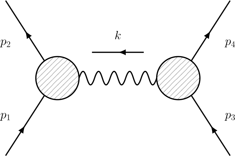
Figure 6: 4-pt amplitude. Figure reproduced from Ref. [100]

$$\mathcal{M}_{4}^{(s_{A},s_{B})}(p_{1},-p_{2},p_{3},-p_{4})=\sum_{h=\pm}\mathcal{M}_{3}^{(s_{A})}(p_{1},-p_{2},k^{h})\dfrac{-1}{t}\mathcal{M}_{3}^{(s_{B})}(p_{3},-p_{4},k^{-h})+\mathcal{O}(t^{0})=$$

$$\qquad\quad=\frac{-(\kappa/2)^{2}}{m_{A}^{2s_{A}-2}m_{B}^{2s_{B}-2}t}\Bigl{(}x_{A}^{2}x_{B}^{-2}\langle\mathbf{2}\mathbf{1}\rangle^{\odot 2s_{A}}[\mathbf{4}\mathbf{3}]^{\odot 2s_{B}}+x_{A}^{-2}x_{B}^{2}[\mathbf{2}\mathbf{1}]^{\odot 2s_{A}}\langle\mathbf{4}\mathbf{3}\rangle^{\odot 2s_{B}}\Bigr{)}+\mathcal{O}(t^{0})\,.$$ (7.1)

It is now convenient to introduce the following kinematic variables

$$x_{A}/x_{B}=\gamma(1-v)\,,\quad x_{B}/x_{A}=\gamma(1+v)\,,\quad\text{with}\quad\gamma=\frac{1}{\sqrt{1-v^{2}}}=\dfrac{p_{A}\cdot p_{B}}{m_{A}m_{B}}=u_{A}\cdot u_{B}\,.$$ (7.2)

Following the procedure outlined in Sec. 4.4, we can thus write:

$$\mathcal{M}_{4}^{(s_{A},s_{B})} =\frac{-(\kappa/2)^{2}\gamma^{2}}{m_{A}^{2s_{A}-2}m_{B}^{2s_{B}-2}t}\,\times$$

$$\times\Bigl{(}(1-v)^{2}\{U_{12}\langle\mathbf{1}|\}^{\odot 2s_{A}}e^{-k\cdot a_{A}}|\mathbf{1}\rangle^{\odot 2s_{A}}\{U_{34}[\mathbf{3}|\}^{\odot 2s_{B}}e^{-k\cdot a_{B}}|\mathbf{3}]^{\odot 2s_{B}}+$$ (7.3)

$$\qquad+(1+v)^{2}\{U_{12}[\mathbf{1}|\}^{\odot 2s_{A}}e^{k\cdot a_{A}}|\mathbf{1}]^{\odot 2s_{A}}\{U_{34}\langle\mathbf{3}|\}^{\odot 2s_{B}}e^{k\cdot a_{B}}|\mathbf{3}\rangle^{\odot 2s_{B}}\Bigr{)}+\mathcal{O}(t^{0})\,.$$

It is now useful to perform a manipulation of these exponentials to obtain a more convenient expression. We recall that on the pole kinematics, $k^{2}=0$; furthermore, due to the transversality of the exchange momentum, $p_{A}\cdot k=p_{B}\cdot k=0$, and by the spin supplementary condition (SSC), $p_{A}\cdot a_{A}=p_{B}\cdot a_{B}=0$.
Therefore the following relations hold true :

$$i\epsilon_{\mu\nu\rho\sigma}p_{A}^{\mu}p_{B}^{\nu}k^{\rho}a_{A}^{\sigma}=m_{A}m_{B}\gamma v(k\cdot a_{A})\,,\quad i\epsilon_{\mu\nu\rho\sigma}p_{A}^{\mu}p_{B}^{\nu}k^{\rho}a_{B}^{\sigma}=m_{A}m_{B}\gamma v(k\cdot a_{B})\,.$$ (7.4)

Hence, if we define

$$w^{\mu\nu}=\frac{2p_{A}^{[\mu}p_{B}^{\nu]}}{m_{A}m_{B}\gamma v}\,,\qquad[w*a]_{\mu}=\frac{1}{2}\epsilon_{\mu\nu\alpha\beta}w^{\alpha\beta}a^{\nu}\,,$$ (7.5)

and strip the unitary transition factors $U_{12}^{\odot 2s_{A}}$ and $U_{34}^{\odot 2s_{B}}$ via the GEV, we obtain the classical limit of the scattering amplitude Eq. (7.1) as

$$\langle\mathcal{M}_{4}(k)\rangle=-\Big{(}\frac{\kappa}{2}\Big{)}^{\!2}\frac{m_{A}^{2}m_{B}^{2}}{k^{2}}\gamma^{2}\sum_{\pm}(1\pm v)^{2}\exp[{\pm i}\bigl{(}k\cdot(w*a_{0})\bigr{)}]\,,$$ (7.6)

where $a_{0}^{\mu}=a_{A}^{\mu}+a_{B}^{\mu}$ is the total spin pseudo-vector.

7.2 Five-point Amplitude

In this section, I will compute the five-point amplitude .
Before delving into the full calculations, I will first review and summarize key results from the previous sections.

7.2.1 Preliminaries

Our starting point is the 4-point amplitude in Fig. (7):

$$\mathcal{M}_{4}^{s_{A},s_{B}}(p_{1},\,p_{2},-p_{3},-p_{4}) =\frac{8\pi G}{m_{A}^{2s_{A}-2}m_{B}^{2s_{B}-2}(p_{1}+p_{3})^{2}}\,\times$$

$$\times\big{(}\gamma^{2}(1-v)^{2}\langle\mathbf{3}\mathbf{1}\rangle^{2s_{A}}[\mathbf{4}\mathbf{2}]^{2s_{B}}+\gamma^{2}(1+v)^{2}[\mathbf{3}\mathbf{1}]^{2s_{A}}\langle\mathbf{4}\mathbf{2}\rangle^{2s_{B}}\big{)}\,,$$

where we work with all external momenta incoming and we have defined

$$\gamma=\dfrac{1}{\sqrt{1-v^{2}}}=\dfrac{p_{1}\!\cdot p_{2}}{m_{1}m_{2}}$$

.

Figure 7: Four-point amplitude with all incoming external momenta

To simplify the calculations, I will restrict to the case where the particle A is spinless, i.e. $s_{A}=0$. The amplitude then becomes:

$$\mathcal{M}_{4}^{0,s_{B}}(p_{1},\,p_{2},\,p_{3},\,p_{4})=\frac{8\pi Gm_{A}^{2}}{m_{B}^{2s_{B}-2}(p_{1}+p_{3})^{2}}\big{(}\gamma^{2}(1-v)^{2}[\mathbf{4}\mathbf{2}]^{2s_{B}}+\gamma^{2}(1+v)^{2}\langle\mathbf{4}\mathbf{2}\rangle^{2s_{B}}\big{)}$$ (7.7)

It is also convenient to define the function $I_{\pm}(p_{1}\cdot p_{2})\equiv\gamma^{2}(1\pm v)^{2}$. So,

$$\mathcal{M}_{4}^{0,s_{B}}(p_{1},\,p_{2},\,p_{3},\,p_{4})=\frac{8\pi Gm_{A}^{2}}{m_{B}^{2s_{B}-2}(p_{1}+p_{3})^{2}}\big{(}I_{-}(p_{1}\cdot p_{2})[\mathbf{4}\mathbf{2}]^{2s_{B}}+I_{+}(p_{1}\cdot p_{2})\langle\mathbf{4}\mathbf{2}\rangle^{2s_{B}}\big{)}$$ (7.8)

As outlined earlier, our aim is to apply the soft theorems discussed in Sec. 5 to derive the five-point amplitude with an emitted graviton starting from the four-point amplitude in Eq. (7.8).
Our strategy consists of shifting the four-point amplitude in the soft limit, $\epsilon\to 0$; then, multiplying it by the appropriate soft factors, we are able to reconstruct the five-point amplitude in the soft limit, where the additional leg corresponds to the soft graviton, labeled as particle $5$.
This approach is somewhat unconventional, as the soft limit is typically used to study the infrared behavior of an amplitude. In such cases, one generally starts with a higher-point amplitude and expands it to express it as a lower-point amplitude multiplied by soft factors. However, by utilizing Eq. (5.37), we can reverse this process, provided we remain consistent with our definition of the shifts.

The natural BCFW shifts we want to use are the ones in Eq. (5.10):

$$\hat{p}_{5}=\epsilon p_{5}-zq_{5}\,,\quad\hat{p}_{1}=p_{1}-\frac{(\epsilon-1)(p_{5}p_{3})-z(q_{5}p_{3})}{q_{1}p_{3}}q_{1}\,,\quad\hat{p}_{3}=p_{3}-\frac{(\epsilon-1)(p_{5}p_{1})-z(q_{5}p_{1})}{q_{3}p_{1}}q_{3}\,,$$ (7.9)

where $q_{5}$, $q_{1}$, $q_{3}$ are four-vectors satisfying

$$q_{5}^{2}=q_{1}^{2}=q_{3}^{2}=q_{5}p_{5}=q_{1}p_{1}=q_{3}p_{3}=0\,,\qquad q_{1}p_{5}=q_{3}p_{5}=q_{1}q_{5}=q_{3}q_{5}=q_{1}q_{3}=0\,.$$ (7.10)

Once again, we choose the the shift vectors $q$ as

$$q_{5}\sigma=y\tilde{\lambda}_{5}\,,\qquad q_{1}\sigma=p_{1}\sigma\tilde{\lambda}_{5}\tilde{\lambda}_{5}\,,\qquad q_{3}\sigma=p_{3}\sigma\tilde{\lambda}_{5}\tilde{\lambda}_{5}\,.$$ (7.11)

We recall that at the spinor level, this shift is achieved by promoting the momenta to be complex, thereby making the holomorphic and antiholomorphic spinors as independent. The shift is then implemented as follows:

$$\{5\bar{\mathbf{1}}\bar{\mathbf{3}}\}\mathrel{\mathop{\mathchar 58\relax}}\qquad\lambda_{5}^{z} =\epsilon\lambda_{5}-zy\,,$$

$$\tilde{\chi}_{1}^{z} =\tilde{\chi}_{1}+\frac{(\epsilon-1)\langle 5p_{3}5]-z\langle yp_{3}5]}{[5p_{1}p_{3}5]}[\mathbf{1}5]\tilde{\lambda}_{5}\,,$$

$$\tilde{\chi}_{3}^{z} =\tilde{\chi}_{3}-\frac{(\epsilon-1)\langle 5p_{1}5]-z\langle yp_{1}5]}{[5p_{1}p_{3}5]}[\mathbf{3}5]\tilde{\lambda}_{5}\,,$$ (7.12)

while keeping all other spinors fixed.
The poles $z_{l}$ are located at $\hat{P}_{5l}^{2}\big{|}_{z=z_{l}}-m_{l}^{2}=0$, so

$$z_{l}=\epsilon\dfrac{p_{5}\cdot p_{l}}{q_{5}\cdot p_{l}}=\epsilon\dfrac{\langle 5p_{l}5]}{\langle yp_{l}5]}\,,$$ (7.13)

and the shifted spinors evaluated at the poles location are:

$$\lambda_{5}^{z_{l}} =\epsilon\frac{\langle y5\rangle}{\langle yp_{l}5]}p_{l}\sigma\tilde{\lambda}_{5}\,,$$

$$\tilde{\chi}_{1}^{z_{l}} =\tilde{\chi}_{1}-\frac{2p_{5}p_{3}}{[5p_{1}p_{3}5]}[\mathbf{1}5]\tilde{\lambda}_{5}+\epsilon\frac{\langle y5\rangle[5p_{3}p_{l}5]}{\langle yp_{l}5][5p_{1}p_{3}5]}[\mathbf{1}5]\tilde{\lambda}_{5}\,,$$ (7.14)

$$\tilde{\chi}_{3}^{z_{l}} =\tilde{\chi}_{3}+\frac{2p_{5}p_{1}}{[5p_{1}p_{3}5]}[\mathbf{3}5]\tilde{\lambda}_{5}-\epsilon\frac{\langle y5\rangle[5p_{1}p_{l}5]}{\langle yp_{l}5][5p_{1}p_{3}5]}[\mathbf{3}5]\tilde{\lambda}_{5}\,.$$

Finally we can rewrite $\hat{P}_{5l}\sigma\big{|}_{z_{l}}$, that being evaluated at the poles is on-shell, as

$$\hat{P}_{5l}\sigma|_{z_{l}}=p_{l}\sigma+\epsilon\dfrac{\langle y5\rangle}{\langle yp_{l}5]}p_{l}\sigma\tilde{\lambda}_{5}\tilde{\lambda}_{5}\,,\,\,\,\Rightarrow\,\,\,\chi_{5l}=\chi_{l}\,,\quad\tilde{\chi}_{5l}=\tilde{\chi}_{l}+\epsilon\frac{\langle y5\rangle}{\langle yp_{l}5]}[\mathbf{l}5]\tilde{\lambda}_{5}\,,\quad l\neq 1,3,$$

$$\hat{P}_{51}\sigma|_{z_{1}}=p_{1}\sigma-\frac{2p_{5}p_{3}}{[5p_{1}p_{3}5]}p_{1}\sigma\tilde{\lambda}_{5}\tilde{\lambda}_{5}\,,\,\Rightarrow\,\chi_{51}=\chi_{1}\,,\quad\tilde{\chi}_{51}=\tilde{\chi}_{1}-\frac{2p_{5}p_{3}}{[5p_{1}p_{3}5]}[\mathbf{1}5]\tilde{\lambda}_{5}\,,$$ (7.15)

$$\hat{P}_{53}\sigma|_{z_{3}}=p_{3}\sigma-\frac{2p_{5}p_{1}}{[5p_{1}p_{3}5]}p_{3}\sigma\tilde{\lambda}_{5}\tilde{\lambda}_{5}\,,\,\Rightarrow\,\chi_{53}=\chi_{3}\,,\quad\tilde{\chi}_{53}=\tilde{\chi}_{1}-\frac{2p_{5}p_{1}}{[5p_{1}p_{3}5]}[\mathbf{3}5]\tilde{\lambda}_{5}\,.$$

Using now the soft theorems discussed in Sec. 5 we have:

$$\hat{\mathcal{M}}^{0,\epsilon}_{5}(\mathbf{1},\mathbf{2},\mathbf{3},\mathbf{4},5_{h}^{+})=\bigg{\{}\frac{1}{\epsilon^{3}}S_{+2}^{(0)}+\frac{1}{\epsilon^{2}}S_{+2}^{(1)}+\frac{1}{\epsilon}S_{+2}^{(0)}\bigg{\}}\hat{\mathcal{M}}^{0,0}_{4}(\hat{\mathbf{1}},\mathbf{2},\hat{\mathbf{3}},\mathbf{4})+\mathcal{O}(\epsilon^{0})\,,$$ (7.16)

where

$$S^{(0)}_{+2}=\frac{\kappa}{2}\sum_{l=1}^{4}\frac{\langle yp_{l}5]^{2}}{(2p_{5}\cdot p_{l})\langle 5y\rangle^{2}}\,,\quad S^{(1)}_{+2}=\frac{\kappa}{2}\sum_{l=1}^{4}\frac{\langle yp_{l}5]}{(2p_{5}\cdot p_{l})\langle 5y\rangle}\tilde{\mathcal{D}}_{l}\,,\quad S^{(2)}_{+2}=\frac{\kappa}{4}\sum_{l=1}^{4}\frac{1}{4p_{5}\cdot p_{l}}\tilde{\mathcal{D}}_{l}\tilde{\mathcal{D}}_{l}\,,$$ (7.17)

and we have defined the quantities

$$\tilde{\mathcal{D}}_{l}=\tilde{d}_{l}+\frac{[5p_{3}p_{l}5]}{[5p_{1}p_{3}5]}[5\mathbf{1}][5\frac{\partial}{\partial\tilde{\chi}_{1}}]-\frac{[5p_{1}p_{l}5]}{[5p_{1}p_{3}5]}[5\mathbf{3}][5\frac{\partial}{\partial\tilde{\chi}_{3}}]\,,\qquad\tilde{d}_{l}=[5\mathbf{l}][5\frac{\partial}{\partial\tilde{\chi}_{l}}]\,,$$ (7.18)

with $\tilde{\mathcal{D}}_{l}=0$ for l = 1, 3.

Notice that for $\epsilon=0$,

$$\hat{P}_{5l}\sigma\big{|}_{z_{l},\epsilon=0}=p_{l}\sigma\big{|}_{\epsilon=0}\,,\qquad\tilde{\chi}_{1}^{z_{l}}\big{|}_{\epsilon=0}=\tilde{\chi}_{1}-\frac{2p_{5}p_{3}}{[5p_{1}p_{3}5]}[\mathbf{1}5]\tilde{\lambda}_{5}\,,\qquad\tilde{\chi}_{3}^{z_{l}}\big{|}_{\epsilon=0}=\tilde{\chi}_{3}+\frac{2p_{5}p_{1}}{[5p_{1}p_{3}5]}[\mathbf{3}5]\tilde{\lambda}_{5}\,.$$ (7.19)

7.2.2 Explicit soft factors

I will now compute Eq. (7.16) explicitly.
First, I will shift the four-point amplitude Eq. (7.8) to obtain its shifted version, $\hat{\mathcal{M}}^{0,0}$. Note that the trivial shift corresponds to $(0,1)$, not $(0,0)$. Therefore, to transition from Eq. (7.8) to its shifted version, I will apply the shift to the momenta $p_{1}\to\hat{p}_{1}$ and $p_{3}\to\hat{p}_{3}$:

$$\hat{\mathcal{M}}_{4}^{0,s_{B}}(\hat{p}_{1},\,p_{2},\,\hat{p}_{3},\,p_{4})\Big{|}_{\epsilon=0}=\frac{8\pi Gm_{A}^{2}}{m_{B}^{2s_{B}-2}(p_{1}+p_{3})^{2}}\big{(}\hat{I}_{-}(\hat{p}_{1}\cdot p_{2})[\mathbf{4}\mathbf{2}]^{2s_{B}}+\hat{I}_{+}(\hat{p}_{1}\cdot p_{2})\langle\mathbf{4}\mathbf{2}\rangle^{2s_{B}}\big{)}$$ (7.20)

Let us now focus on the functions $\hat{I}_{\pm}(\hat{p}_{1}\cdot p_{2})$ and see how they are related to their un-shifted version $I_{\pm}(p_{1}\cdot p_{2})$. To this end we find convenient to write $I_{\pm}(p_{1}\cdot p_{2})$ explicitly as:

$$I_{\pm}(p_{1}\cdot p_{2}) =\gamma^{2}(1\pm v)^{2}=$$ (7.21)

$$=\left(\frac{p_{1}\cdot p_{2}}{m_{1}m_{2}}\left(1\pm\sqrt{1-\frac{m_{1}^{2}m_{2}^{2}}{(p_{1}\cdot p_{2})^{2}}}\right)\right)^{2}=\left(\frac{p_{1}\cdot p_{2}\pm\sqrt{(p_{1}\cdot p_{2})^{2}-m_{1}^{2}m_{2}^{2}}}{m_{1}m_{2}}\right)^{2}\,.$$

Thus $\hat{I}_{\pm}(\hat{p}_{1}\cdot p_{2})$ is nothing but:

$$I_{\pm}(\hat{p}_{1}\cdot p_{2})=\left(\frac{\hat{p}_{1}\cdot p_{2}\pm\sqrt{(\hat{p}_{1}\cdot p_{2})^{2}-m_{1}^{2}m_{2}^{2}}}{m_{1}m_{2}}\right)^{2}\,.$$ (7.22)

We can now easily express the product $\hat{p}_{1}\cdot p_{2}$ in terms of the un-shifted spinors using Eq. (7.19) and the identity:

$$\hat{p}_{1}\cdot p_{2}=\frac{1}{2}\langle\hat{\mathbf{1}}\mathbf{2}\rangle[\mathbf{2}\hat{\mathbf{1}}]\,.$$ (7.23)

Therefore,

$$\hat{p}_{1}\cdot p_{2} =\frac{1}{2}\langle\hat{\mathbf{1}}\mathbf{2}\rangle[\mathbf{2}\hat{\mathbf{1}}]=$$ (7.24)

$$=\frac{1}{2}\langle{\mathbf{1}}\mathbf{2}\rangle[\mathbf{2}{\mathbf{1}}]-\frac{p_{5}p_{3}}{[5p_{1}p_{3}5]}\langle\mathbf{1}\mathbf{2}\rangle[\mathbf{1}5][\mathbf{2}5]=p_{1}\cdot p_{2}-\frac{p_{5}p_{3}}{[5p_{1}p_{3}5]}[\mathbf{1}5]\langle\mathbf{1}\mathbf{2}\rangle[\mathbf{2}5]\,.$$

We are now ready to compute the desired five-point amplitude.
For simplicity, I will work out the terms in Eq. (7.16) one by one, starting with $S^{(0)}_{+2}$. Remembering that $\kappa^{2}=32\pi G$, we have:

$$\dfrac{1}{\epsilon^{3}}S_{+2}^{(0)}\hat{\mathcal{M}}^{0,0}_{4}(\hat{\mathbf{1}},\mathbf{2},\hat{\mathbf{3}},\mathbf{4}) =$$

$$=\dfrac{1}{\epsilon^{3}}\left(\dfrac{\kappa}{2}\right)^{\!3}\dfrac{m_{A}^{2}}{m_{B}^{2s_{B}-2}(p_{1}+p_{3})^{2}}\,\times$$ (7.25)

$$\times\sum_{l=1}^{4}\frac{\langle yp_{l}5]^{2}}{(2p_{5}\cdot p_{l})\langle 5y\rangle^{2}}\left(\hat{I}_{-}(\hat{p}_{1}\cdot p_{2})[\mathbf{4}\mathbf{2}]^{2s_{B}}+\hat{I}_{+}(\hat{p}_{1}\cdot p_{2})\langle\mathbf{4}\mathbf{2}\rangle^{2s_{B}}\right)\,.$$

I then compute the term $S^{(1)}_{+2}$:

$$\dfrac{1}{\epsilon^{2}}S_{+2}^{(1)}\hat{\mathcal{M}}^{0,0}_{4}(\hat{\mathbf{1}},\mathbf{2},\hat{\mathbf{3}},\mathbf{4}) =$$

$$=\dfrac{1}{\epsilon^{2}}\left(\frac{\kappa}{2}\right)^{\!3}\dfrac{m_{A}^{2}}{m_{B}^{2s_{B}-2}(p_{1}+p_{3})^{2}}\,\times$$ (7.26)

$$\times\sum_{l=1}^{4}\dfrac{\langle yp_{l}5]}{(2p_{5}\cdot p_{l})\langle 5y\rangle}\tilde{\mathcal{D}}_{l}\left(\hat{I}_{-}(\hat{p}_{1}\cdot p_{2})[\mathbf{4}\mathbf{2}]^{2s_{B}}+\hat{I}_{+}(\hat{p}_{1}\cdot p_{2})\langle\mathbf{4}\mathbf{2}\rangle^{2s_{B}}\right)\,.$$

Notice now that the operator $\tilde{\mathcal{D}}_{l}$ is simply the realization of the derivative $\frac{\partial}{\partial\epsilon}$, hence it behaves as the usual derivative, in the sense that it satisfies the usual Leibniz product rule and the chain rule. Hence,

$$\tilde{\mathcal{D}}_{l}\left(\hat{I}_{-}(\hat{p}_{1}\cdot p_{2})[\mathbf{4}\mathbf{2}]^{2s_{B}}+\hat{I}_{+}(\hat{p}_{1}\cdot p_{2})\langle\mathbf{4}\mathbf{2}\rangle^{2s_{B}}\right)=$$ (7.27)

$$\qquad\qquad=\left(\tilde{\mathcal{D}}_{l}(\hat{I}_{-}(\hat{p}_{1}\cdot p_{2})\right)[\mathbf{4}\mathbf{2}]^{2s_{B}}+\hat{I}_{-}(\hat{p}_{1}\cdot p_{2})\left(\tilde{\mathcal{D}}_{l}[\mathbf{4}\mathbf{2}]^{2s_{B}}\right)+\left(\tilde{\mathcal{D}}_{l}\hat{I}_{+}(\hat{p}_{1}\cdot p_{2})\right)\langle\mathbf{4}\mathbf{2}\rangle^{2s_{B}}\,+$$

$$\hskip 85.35826pt+\hat{I}_{+}(\hat{p}_{1}\cdot p_{2})\left(\tilde{\mathcal{D}}_{l}\langle\mathbf{4}\mathbf{2}\rangle^{2s_{B}}\right)$$

Let us examine each of these contributions individually. Consider the first and the third terms in Eq. (7.27):

$$\tilde{\mathcal{D}}_{l}(\hat{I}_{\pm}(\hat{p}_{1}\cdot p_{2}))=\frac{\partial\big{(}\hat{I}_{\pm}(\hat{p}_{1}\cdot p_{2})\big{)}}{\partial(\hat{p}_{1}\cdot p_{2})}\tilde{\mathcal{D}}_{l}(\hat{p}_{1}\cdot p_{2})\equiv\hat{I}^{\prime}_{\pm}(\hat{p}_{1}\cdot p_{2})\tilde{\mathcal{D}}_{l}(\hat{p}_{1}\cdot p_{2})\,,$$ (7.28)

where we have defined the function

$$\hat{I}^{\prime}_{\pm}(\hat{p}_{1}\cdot p_{2})\equiv\frac{\partial\big{(}\hat{I}_{\pm}(\hat{p}_{1}\cdot p_{2})\big{)}}{\partial(\hat{p}_{1}\cdot p_{2})}=\pm\frac{2}{m_{1}^{2}m_{2}^{2}}\dfrac{\left(\hat{p}_{1}\cdot p_{2}\pm\sqrt{(\hat{p}_{1}\cdot p_{2})^{2}-m_{1}^{2}m_{2}^{2}}\right)^{2}}{\sqrt{(\hat{p}_{1}\cdot p_{2})^{2}-m_{1}^{2}m_{2}^{2}}}$$ (7.29)

We recall that $\tilde{\mathcal{D}}_{l}=0$ for $l=1,3$; so we are left to compute just $\tilde{\mathcal{D}}_{2}(\hat{p}_{1}\cdot p_{2})$ and $\tilde{\mathcal{D}}_{4}(\hat{p}_{1}\cdot p_{2})$. To compute such derivatives, I will use the parity conjugate version of the identity in Eq. (4.55), that I rewrite below for convenience:

$$[k\frac{\partial}{\partial\tilde{\chi}_{p}^{b}}]|p^{a}]=\delta^{a}_{b}|k]\,.$$ (7.30)

So,

$$\tilde{\mathcal{D}}_{2}(\hat{p}_{1}\cdot p_{2}) =\left([5\mathbf{2}][5\frac{\partial}{\partial\tilde{\chi}_{2}}]+\dfrac{[5p_{3}p_{2}3]}{[5p_{1}p_{3}5]}[5\mathbf{1}][5\frac{\partial}{\partial\tilde{\chi}_{1}}]-\dfrac{[5p_{1}p_{2}5]}{[5p_{1}p_{3}5]}[5\mathbf{3}][5\frac{\partial}{\partial\tilde{\chi}_{3}}]\right)\left(\frac{1}{2}\langle\mathbf{1}\mathbf{2}\rangle[\mathbf{2}\hat{\mathbf{1}}]\right)=$$

$$=\dfrac{1}{2}[5\mathbf{1}]\langle\mathbf{1}\mathbf{2}\rangle[\mathbf{2}5]+\dfrac{1}{2}\dfrac{[5p_{3}p_{2}5]}{[5p_{1}p_{3}5]}[5\mathbf{1}]\langle\mathbf{1}\mathbf{2}\rangle[\mathbf{2}5]=$$ (7.31a)

$$=\frac{1}{2}[5\mathbf{1}]\langle\mathbf{1}\mathbf{2}\rangle[\mathbf{2}5]\left(1+\dfrac{[5p_{3}p_{2}5]}{[5p_{1}p_{3}5]}\right)\,,$$

$$\tilde{\mathcal{D}}_{4}(\hat{p}_{1}\cdot p_{2}) =\left([5\mathbf{4}][5\frac{\partial}{\partial\tilde{\chi}_{4}}]+\dfrac{[5p_{3}p_{4}3]}{[5p_{1}p_{3}5]}[5\mathbf{1}][5\frac{\partial}{\partial\tilde{\chi}_{1}}]-\dfrac{[5p_{1}p_{4}5]}{[5p_{1}p_{3}5]}[5\mathbf{3}][5\frac{\partial}{\partial\tilde{\chi}_{3}}]\right)\left(\frac{1}{2}\langle\mathbf{1}\mathbf{2}\rangle[\mathbf{2}\hat{\mathbf{1}}]\right)=$$

$$=\dfrac{1}{2}[5\mathbf{1}]\langle\mathbf{1}\mathbf{2}\rangle[\mathbf{2}5]\dfrac{[5p_{3}p_{4}5]}{[5p_{1}p_{3}5]}\,.$$ (7.31b)

Consider now the second term in Eq. (7.27). In this case the derivative acts only on the un-shifted spinors, so we simply have:

$$\tilde{\mathcal{D}}_{2}[\mathbf{4}\mathbf{2}]^{2s_{B}} =\left([5\mathbf{2}][5\frac{\partial}{\partial\tilde{\chi}_{2}}]\right)[\mathbf{4}\mathbf{2}]^{2s_{B}}=\tilde{d}_{2}[\mathbf{4}\mathbf{2}]^{2s_{B}}$$ (7.32a)

$$\tilde{\mathcal{D}}_{4}[\mathbf{4}\mathbf{2}]^{2s_{B}} =\left([5\mathbf{4}][5\frac{\partial}{\partial\tilde{\chi}_{4}}]\right)[\mathbf{4}\mathbf{2}]^{2s_{B}}=\tilde{d}_{4}[\mathbf{4}\mathbf{2}]^{2s_{B}}$$ (7.32b)

Furthermore, it is straightforward to check that: $\tilde{d}_{2}[\mathbf{4}\mathbf{2}]^{2s_{B}}=-\tilde{d}_{4}[\mathbf{4}\mathbf{2}]^{2s_{B}}$.

At last, consider the fourth term in. in Eq. (7.27). As we are working with complex momenta, holomorphic and anti-holomorphic spinors are completely independent, thus

$$\tilde{\mathcal{D}}_{2}\langle\mathbf{4}\mathbf{2}\rangle^{2s_{B}}=\tilde{\mathcal{D}}_{4}\langle\mathbf{4}\mathbf{2}\rangle^{2s_{B}}=0\,.$$ (7.33)

We can now finally substitute Eq. (7.27) in Eq. (7.2.2) to get:

$$\dfrac{1}{\epsilon^{2}}S_{+2}^{(1)}\hat{\mathcal{M}}^{0,0}_{4}(\hat{\mathbf{1}},\mathbf{2},\hat{\mathbf{3}},\mathbf{4}) =$$ (7.34)

$$=\dfrac{1}{\epsilon^{2}}\left(\dfrac{\kappa}{2}\right)^{\!3}\dfrac{m_{A}^{2}}{m_{B}^{2s_{B}-2}(p_{1}+p_{3})^{2}}\,\times$$

$$\times\Biggl{\{}\dfrac{\langle yp_{2}5]}{(2p_{5}\cdot p_{2})\langle 5y\rangle}\biggl{(}\hat{I}^{\prime}_{-}(\hat{p}_{1}\cdot p_{2})\tilde{\mathcal{D}}_{2}(\hat{p}_{1}\cdot p_{2})[\mathbf{4}\mathbf{2}]^{2s_{B}}+\hat{I}_{-}(\hat{p}_{1}\cdot p_{2})\big{(}\tilde{d}_{2}[\mathbf{4}\mathbf{2}]^{2s_{B}}\big{)}\,+$$

$$\hskip 71.13188pt+\hat{I}^{\prime}_{+}(\hat{p}_{1}\cdot p_{2})\tilde{\mathcal{D}}_{2}(\hat{p}_{1}\cdot p_{2})\langle\mathbf{4}\mathbf{2}\rangle^{2s_{B}}\biggr{)}\,+$$

$$+\dfrac{\langle yp_{4}5]}{(2p_{5}\cdot p_{4})\langle 5y\rangle}\biggl{(}\hat{I}^{\prime}_{-}(\hat{p}_{1}\cdot p_{2})\tilde{\mathcal{D}}_{4}(\hat{p}_{1}\cdot p_{2})[\mathbf{4}\mathbf{2}]^{2s_{B}}+\hat{I}_{-}(\hat{p}_{1}\cdot p_{2})\big{(}\tilde{d}_{4}[\mathbf{4}\mathbf{2}]^{2s_{B}}\big{)}\,+$$

$$\hskip 85.35826pt+\hat{I}^{\prime}_{+}(\hat{p}_{1}\cdot p_{2})\tilde{\mathcal{D}}_{4}(\hat{p}_{1}\cdot p_{2})\langle\mathbf{4}\mathbf{2}\rangle^{2s_{B}}\biggr{)}\,\Biggr{\}}=$$

$$=\dfrac{1}{\epsilon^{2}}\left(\dfrac{\kappa}{2}\right)^{\!3}\dfrac{m_{A}^{2}}{m_{B}^{2s_{B}-2}(p_{1}+p_{3})^{2}}\,\times$$

$$\times\Biggl{\{}\left[\dfrac{\langle yp_{2}5]}{(4p_{5}\cdot p_{2})\langle 5y\rangle}\left(1+\dfrac{[5p_{3}p_{2}5]}{[5p_{1}p_{3}5]}\right)+\dfrac{\langle yp_{4}5]}{(4p_{5}\cdot p_{4})\langle 5y\rangle}\dfrac{[5p_{3}p_{4}5]}{[5p_{1}p_{3}5]}\right][5\mathbf{1}]\langle\mathbf{1}\mathbf{2}\rangle[\mathbf{2}5]\,\times$$

$$\times\left(\hat{I}^{\prime}_{-}(\hat{p}_{1}\cdot p_{2})[\mathbf{4}\mathbf{2}]^{2s_{B}}+\hat{I}^{\prime}_{+}(\hat{p}_{1}\cdot p_{2})\langle\mathbf{4}\mathbf{2}\rangle^{2s_{B}}\right)\,+$$

$$+\left[\dfrac{\langle yp_{2}5]}{(2p_{5}\cdot p_{2})\langle 5y\rangle}-\dfrac{\langle yp_{4}5]}{(2p_{5}\cdot p_{4})\langle 5y\rangle}\right]\hat{I}_{-}(\hat{p}_{1}\cdot p_{2})\,\big{(}\tilde{d}_{2}[\mathbf{4}\mathbf{2}]^{2s_{B}}\big{)}\Biggr{\}}\,.$$

I then compute the term $S^{(2)}_{+2}$:

$$\dfrac{1}{\epsilon}S_{+2}^{(2)}\hat{\mathcal{M}}^{0,0}_{4}(\hat{\mathbf{1}},\mathbf{2},\hat{\mathbf{3}},\mathbf{4}) =$$ (7.35)

$$=\dfrac{1}{\epsilon}\left(\dfrac{\kappa}{2}\right)^{\!3}\dfrac{m_{A}^{2}}{m_{B}^{2s_{B}-2}(p_{1}+p_{3})^{2}}\sum_{l=1}^{4}\frac{1}{4p_{5}\cdot p_{l}}\tilde{\mathcal{D}}_{l}\tilde{\mathcal{D}}_{l}\left(\hat{I}_{-}(\hat{p}_{1}\cdot p_{2})[\mathbf{4}\mathbf{2}]^{2s_{B}}+\hat{I}_{+}(\hat{p}_{1}\cdot p_{2})\langle\mathbf{4}\mathbf{2}\rangle^{2s_{B}}\right)\,.$$

Let us now focus on this second derivative:

$$\tilde{\mathcal{D}}_{l}\left(\tilde{\mathcal{D}}_{l}\left(\hat{I}_{-}(\hat{p}_{1}\cdot p_{2})[\mathbf{4}\mathbf{2}]^{2s_{B}}+\hat{I}_{+}(\hat{p}_{1}\cdot p_{2})\langle\mathbf{4}\mathbf{2}\rangle^{2s_{B}}\right)\right)=$$ (7.36)

$$\hskip 56.9055pt=\tilde{\mathcal{D}}_{l}\biggl{(}\hat{I}^{\prime}_{-}(\hat{p}_{1}\cdot p_{2})\tilde{\mathcal{D}}_{l}(\hat{p}_{1}\cdot p_{2})[\mathbf{4}\mathbf{2}]^{2s_{B}}+\hat{I}_{-}(\hat{p}_{1}\cdot p_{2})\left(\tilde{d}_{l}[\mathbf{4}\mathbf{2}]^{2s_{B}}\right)\,+$$

$$\hskip 142.26378pt+\hat{I}^{\prime}_{+}(\hat{p}_{1}\cdot p_{2})\tilde{\mathcal{D}}_{l}(\hat{p}_{1}\cdot p_{2})\langle\mathbf{4}\mathbf{2}\rangle^{2s_{B}}\biggr{)}=$$

$$\hskip 56.9055pt=\hat{I}^{\prime\prime}_{-}(\hat{p}_{1}\cdot p_{2})\left(\tilde{\mathcal{D}}_{l}(\hat{p}_{1}\cdot p_{2})\right)^{\!2}[\mathbf{4}\mathbf{2}]^{2s_{B}}+\hat{I}^{\prime}_{-}(\hat{p}_{1}\cdot p_{2})\,\tilde{\mathcal{D}}_{l}\left(\tilde{\mathcal{D}}_{l}(\hat{p}_{1}\cdot p_{2})\right)[\mathbf{4}\mathbf{2}]^{2s_{B}}\,+$$

$$\hskip 85.35826pt+2\,\hat{I}^{\prime}_{-}(\hat{p}_{1}\cdot p_{2})\tilde{\mathcal{D}}_{l}(\hat{p}_{1}\cdot p_{2})\tilde{d}_{l}[\mathbf{4}\mathbf{2}]^{2s_{B}}+\hat{I}_{-}(\hat{p}_{1}\cdot p_{2})\,\tilde{\mathcal{D}}_{l}\left(\tilde{d}_{l}[\mathbf{4}\mathbf{2}]^{2s_{B}}\right)\,+$$

$$\hskip 85.35826pt+\hat{I}^{\prime\prime}_{+}(\hat{p}_{1}\cdot p_{2})\left(\tilde{\mathcal{D}}_{l}(\hat{p}_{1}\cdot p_{2})\right)^{\!2}\langle\mathbf{4}\mathbf{2}\rangle^{2s_{B}}+\hat{I}^{\prime}_{+}(\hat{p}_{1}\cdot p_{2})\,\tilde{\mathcal{D}}_{l}\left(\tilde{\mathcal{D}}_{l}(\hat{p}_{1}\cdot p_{2})\right)\langle\mathbf{4}\mathbf{2}\rangle^{2s_{B}}\,,$$

where we have defined the function

$$\hat{I}^{\prime\prime}_{\pm}(\hat{p}_{1}\cdot p_{2}) \equiv\frac{\partial{}^{\,2}\big{(}\hat{I}_{\pm}(\hat{p}_{1}\cdot p_{2})\big{)}}{\partial(\hat{p}_{1}\cdot p_{2})^{2}}=$$ (7.37)

$$=\dfrac{2\left(\hat{p}_{1}\cdot p_{2}\pm\sqrt{(\hat{p}_{1}\cdot p_{2})^{2}-m_{1}^{2}m_{2}^{2}}\right)^{2}}{m_{1}^{2}m_{2}^{2}\left[(\hat{p}_{1}\cdot p_{2})^{2}-m_{1}^{2}m_{2}^{2}\right]^{3/2}}\left(2\sqrt{(\hat{p}_{1}\cdot p_{2})^{2}-m_{1}^{2}m_{2}^{2}}\mp\hat{p}_{1}\cdot p_{2}\right)\,.$$

Let’s examine, once again, each of the new contributions individually. Consider the second and and sixth terms in Eq. (7.36):

$$\tilde{\mathcal{D}}_{2}\left(\tilde{\mathcal{D}}_{2}(\hat{p}_{1}\cdot p_{2})\right)=\tilde{\mathcal{D}}_{2}\left(\frac{1}{2}[5\mathbf{1}]\langle\mathbf{1}\mathbf{2}\rangle[\mathbf{2}5]\left(1+\dfrac{[5p_{3}p_{2}5]}{[5p_{1}p_{3}5]}\right)\right)\propto[55]=0\,,$$ (7.38)

$$\tilde{\mathcal{D}}_{4}\left(\tilde{\mathcal{D}}_{4}(\hat{p}_{1}\cdot p_{2})\right)=\tilde{\mathcal{D}}_{4}\left(\dfrac{1}{2}[5\mathbf{1}]\langle\mathbf{1}\mathbf{2}\rangle[\mathbf{2}5]\dfrac{[5p_{3}p_{4}5]}{[5p_{1}p_{3}5]}\right)\propto[55]=0\,.$$

It is worth noting that this outcome is expected: although the amplitude itself has no specific $\epsilon$-dependence, the momentum shifts are linear in $\epsilon$. Given now that $\tilde{\mathcal{D}}_{l}$ is merely the realization via the chain rule of $\frac{\partial}{\partial\epsilon}$, it follows that the second derivative vanishes when acting on (the linear $\epsilon$-dependent term) $\hat{p_{1}}\cdot p_{2}$.

Consider now the fourth term in Eq. (7.36). As for Eq. (7.32) it is straightforward to check that:

$$\begin{gathered}\tilde{\mathcal{D}}_{2}\left(\tilde{d}_{2}[\mathbf{4}\mathbf{2}]^{2s_{B}}\right)=\tilde{d}_{2}\left(\tilde{d}_{2}[\mathbf{4}\mathbf{2}]^{2s_{B}}\right)\,,\qquad\tilde{\mathcal{D}}_{4}\left(\tilde{d}_{4}[\mathbf{4}\mathbf{2}]^{2s_{B}}\right)=\tilde{d}_{4}\left(\tilde{d}_{4}[\mathbf{4}\mathbf{2}]^{2s_{B}}\right)\,,\\ \tilde{d}_{2}\left(\tilde{d}_{2}[\mathbf{4}\mathbf{2}]^{2s_{B}}\right)=\tilde{d}_{4}\left(\tilde{d}_{4}[\mathbf{4}\mathbf{2}]^{2s_{B}}\right)\,.\end{gathered}$$ (7.39)

We can now finally substitute Eq. (7.36) in Eq. (7.35) to get:

$$\dfrac{1}{\epsilon}S_{+2}^{(2)}\hat{\mathcal{M}}^{0,0}_{4}(\hat{\mathbf{1}},\mathbf{2},\hat{\mathbf{3}},\mathbf{4}) =$$ (7.40)

$$=\dfrac{1}{\epsilon}\left(\dfrac{\kappa}{2}\right)^{\!3}\dfrac{m_{A}^{2}}{m_{B}^{2s_{B}-2}(p_{1}+p_{3})^{2}}\,\times$$

$$\times\Biggl{\{}\dfrac{1}{4p_{5}\cdot p_{2}}\biggl{(}\hat{I}^{\prime\prime}_{-}(\hat{p}_{1}\cdot p_{2})\left(\tilde{\mathcal{D}}_{2}(\hat{p}_{1}\cdot p_{2})\right)^{\!2}[\mathbf{4}\mathbf{2}]^{2s_{B}}+2\,\hat{I}^{\prime}_{-}(\hat{p}_{1}\cdot p_{2})\tilde{\mathcal{D}}_{2}(\hat{p}_{1}\cdot p_{2})\tilde{d}_{2}[\mathbf{4}\mathbf{2}]^{2s_{B}}\,+$$

$$+\hat{I}_{-}(\hat{p}_{1}\cdot p_{2})\,\tilde{d}_{2}\left(\tilde{d}_{2}[\mathbf{4}\mathbf{2}]^{2s_{B}}\right)+\hat{I}^{\prime\prime}_{+}(\hat{p}_{1}\cdot p_{2})\left(\tilde{\mathcal{D}}_{2}(\hat{p}_{1}\cdot p_{2})\right)^{\!2}\langle\mathbf{4}\mathbf{2}\rangle^{2s_{B}}\biggr{)}\,+$$

$$+\frac{1}{4p_{5}\cdot p_{4}}\biggl{(}\hat{I}^{\prime\prime}_{-}(\hat{p}_{1}\cdot p_{2})\left(\tilde{\mathcal{D}}_{4}(\hat{p}_{1}\cdot p_{2})\right)^{\!2}[\mathbf{4}\mathbf{2}]^{2s_{B}}+2\,\hat{I}^{\prime}_{-}(\hat{p}_{1}\cdot p_{2})\tilde{\mathcal{D}}_{4}(\hat{p}_{1}\cdot p_{2})\tilde{d}_{4}[\mathbf{4}\mathbf{2}]^{2s_{B}}\,+$$

$$\quad+\hat{I}_{-}(\hat{p}_{1}\cdot p_{2})\,\tilde{d}_{4}\left(\tilde{d}_{4}[\mathbf{4}\mathbf{2}]^{2s_{B}}\right)+\hat{I}^{\prime\prime}_{+}(\hat{p}_{1}\cdot p_{2})\left(\tilde{\mathcal{D}}_{4}(\hat{p}_{1}\cdot p_{2})\right)^{\!2}\langle\mathbf{4}\mathbf{2}\rangle^{2s_{B}}\biggr{)}\Biggr{\}}\,=$$

$$=\dfrac{1}{\epsilon}\left(\dfrac{\kappa}{2}\right)^{\!3}\dfrac{m_{A}^{2}}{m_{B}^{2s_{B}-2}(p_{1}+p_{3})^{2}}\,\times$$

$$\times\Biggl{\{}\Biggl{[}\frac{1}{16p_{5}\cdot p_{2}}\left(1+\dfrac{[5p_{3}p_{2}5]}{[5p_{1}p_{3}5]}\right)^{\!\!2}+\dfrac{1}{16p_{5}\cdot p_{4}}\left(\dfrac{[5p_{3}p_{4}5]}{[5p_{1}p_{3}5]}\right)^{\!\!2}\Biggr{]}\left([5\mathbf{1}]\langle\mathbf{1}\mathbf{2}\rangle[\mathbf{2}5]\right)^{2}\times$$

$$\qquad\times\left(\hat{I}^{\prime\prime}_{-}(\hat{p}_{1}\cdot p_{2})[\mathbf{4}\mathbf{2}]^{2s_{B}}+\hat{I}^{\prime\prime}_{+}(\hat{p}_{1}\cdot p_{2})\langle\mathbf{4}\mathbf{2}\rangle^{2s_{B}}\right)\,+$$

$$+\Biggl{[}\dfrac{1}{4p_{5}\cdot p_{2}}\left(1+\dfrac{[5p_{3}p_{2}5]}{[5p_{1}p_{3}5]}\right)-\dfrac{1}{4p_{5}\cdot p_{4}}\dfrac{[5p_{3}p_{4}5]}{[5p_{1}p_{3}5]}\Biggr{]}[5\mathbf{1}]\langle\mathbf{1}\mathbf{2}\rangle[\mathbf{2}5]\,\times$$

$$\qquad\times\hat{I}^{\prime}_{-}(\hat{p}_{1}\cdot p_{2})\left(\tilde{d}_{2}[\mathbf{4}\mathbf{2}]^{2s_{B}}\right)\,+$$

$$+\left[\dfrac{1}{4p_{5}\cdot p_{2}}+\dfrac{1}{4p_{5}\cdot p_{4}}\right]\hat{I}_{-}(\hat{p}_{1}\cdot p_{2})\left(\tilde{d}_{2}(\tilde{d}_{2}[\mathbf{4}\mathbf{2}]^{2s_{B}})\right)\Biggr{\}}$$

Substituting now Eq. (7.2.2), Eq. (7.34) and Eq. (7.40) in Eq. (7.16), we finally obtain the five-point amplitude in the soft expansion up to sub-sub-leading order:

$$\hat{\mathcal{M}}^{0,\epsilon}_{5}(\mathbf{1},\mathbf{2},\mathbf{3},\mathbf{4},5_{h}^{+}) =\left(\dfrac{\kappa}{2}\right)^{\!3}\dfrac{m_{A}^{2}}{m_{B}^{2s_{B}-2}(p_{1}+p_{3})^{2}}\,\times$$ (7.41)

$$\times\Biggl{\{}\dfrac{1}{\epsilon^{3}}\sum_{l=1}^{4}\frac{\langle yp_{l}5]^{2}}{(2p_{5}\cdot p_{l})\langle 5y\rangle^{2}}\left(\hat{I}_{-}(\hat{p}_{1}\cdot p_{2})[\mathbf{4}\mathbf{2}]^{2s_{B}}+\hat{I}_{+}(\hat{p}_{1}\cdot p_{2})\langle\mathbf{4}\mathbf{2}\rangle^{2s_{B}}\right)\,+$$

$$+\dfrac{1}{\epsilon^{2}}\Biggl{\{}\left[\dfrac{\langle yp_{2}5]}{(4p_{5}\cdot p_{2})\langle 5y\rangle}\left(1+\dfrac{[5p_{3}p_{2}5]}{[5p_{1}p_{3}5]}\right)+\dfrac{\langle yp_{4}5]}{(4p_{5}\cdot p_{4})\langle 5y\rangle}\dfrac{[5p_{3}p_{4}5]}{[5p_{1}p_{3}5]}\right][5\mathbf{1}]\langle\mathbf{1}\mathbf{2}\rangle[\mathbf{2}5]\,\times$$

$$\times\left(\hat{I}^{\prime}_{-}(\hat{p}_{1}\cdot p_{2})[\mathbf{4}\mathbf{2}]^{2s_{B}}+\hat{I}^{\prime}_{+}(\hat{p}_{1}\cdot p_{2})\langle\mathbf{4}\mathbf{2}\rangle^{2s_{B}}\right)\,+$$

$$+\left[\dfrac{\langle yp_{2}5]}{(2p_{5}\cdot p_{2})\langle 5y\rangle}-\dfrac{\langle yp_{4}5]}{(2p_{5}\cdot p_{4})\langle 5y\rangle}\right]\hat{I}_{-}(\hat{p}_{1}\cdot p_{2})\,\big{(}\tilde{d}_{2}[\mathbf{4}\mathbf{2}]^{2s_{B}}\big{)}\Biggr{\}}\,+$$

$$+\dfrac{1}{\epsilon}\Biggl{\{}\Biggl{[}\frac{1}{16p_{5}\cdot p_{2}}\left(1+\dfrac{[5p_{3}p_{2}5]}{[5p_{1}p_{3}5]}\right)^{\!\!2}+\dfrac{1}{16p_{5}\cdot p_{4}}\left(\dfrac{[5p_{3}p_{4}5]}{[5p_{1}p_{3}5]}\right)^{\!\!2}\Biggr{]}\left([5\mathbf{1}]\langle\mathbf{1}\mathbf{2}\rangle[\mathbf{2}5]\right)^{2}\times$$

$$\qquad\times\left(\hat{I}^{\prime\prime}_{-}(\hat{p}_{1}\cdot p_{2})[\mathbf{4}\mathbf{2}]^{2s_{B}}+\hat{I}^{\prime\prime}_{+}(\hat{p}_{1}\cdot p_{2})\langle\mathbf{4}\mathbf{2}\rangle^{2s_{B}}\right)\,+$$

$$+\Biggl{[}\dfrac{1}{4p_{5}\cdot p_{2}}\left(1+\dfrac{[5p_{3}p_{2}5]}{[5p_{1}p_{3}5]}\right)-\dfrac{1}{4p_{5}\cdot p_{4}}\dfrac{[5p_{3}p_{4}5]}{[5p_{1}p_{3}5]}\Biggr{]}[5\mathbf{1}]\langle\mathbf{1}\mathbf{2}\rangle[\mathbf{2}5]\,\times$$

$$\qquad\times\hat{I}^{\prime}_{-}(\hat{p}_{1}\cdot p_{2})\left(\tilde{d}_{2}[\mathbf{4}\mathbf{2}]^{2s_{B}}\right)\,+$$

$$+\left[\dfrac{1}{4p_{5}\cdot p_{2}}+\dfrac{1}{4p_{5}\cdot p_{4}}\right]\hat{I}_{-}(\hat{p}_{1}\cdot p_{2})\left(\tilde{d}_{2}(\tilde{d}_{2}[\mathbf{4}\mathbf{2}]^{2s_{B}})\right)\Biggr{\}}\Biggr{\}}\,.$$

7.2.3 Classical large spin limit

We are now interested in taking the large classical spin limit of the amplitude Eq. (7.41) in order to compute a sensible amplitude. I will follow the works presented in Ref. [100, 103] and discussed in Sec. 4.4, and extend it to the five-point amplitude.

We recall that a consistent picture of spin-induced multipoles of a pointlike particle must be formulated in the particle’s rest frame and that all spin multipoles of the amplitude can be extracted through a finite Lorentz boost which is needed to bridge the gap between two states with different momenta. To start, we note that any two four-vectors $p_{4}$ and $p_{2}$ of equal mass $m$ may be related by the spinorial transformations:

$$|\mathbf{4}^{b}\rangle =U_{24~{}a}^{~{}~{}b}\exp\!\left(\dfrac{i}{m^{2}}p_{2}^{\mu}q^{\nu}\sigma_{\mu\nu}\!\right)|\mathbf{2}^{a}\rangle\,,\qquad|\mathbf{4}^{b}] =U_{24~{}a}^{~{}~{}b}\exp\!\left(\dfrac{i}{m^{2}}p_{2}^{\mu}q^{\nu}\bar{\sigma}_{\mu\nu}\!\right)|\mathbf{2}^{a}]\,,$$ (7.42)

where $U_{24}\text{in}SU(2)$ is a little-group transformation that depends on the specifics of the massive-spinor realization, $q$ is the boost $q\equiv p_{2}+p_{4}$ needed to connect the two spinors. Note that $q^{2}=(p_{2}+p_{4})^{2}=0$ as we are working in the on-shell framework and we are in the center of mass frame of the interactions.
Furthermore, using Eq. (4.74), we write the above exponents as:

$$\frac{i}{m^{2}}p_{2}^{\mu}q^{\nu}\sigma_{\mu\nu,\alpha}^{~{}~{}~{}~{}\;\beta}=q\cdot(a_{B})_{\alpha}^{~{}\beta},\qquad\frac{i}{m^{2}}p_{2}^{\mu}q^{\nu}\bar{\sigma}^{~{}~{}~{}\dot{\alpha}}_{\mu\nu,~{}\dot{\beta}}=-q\cdot(a_{B})^{\dot{\alpha}}_{~{}\,\dot{\beta}}\,$$ (7.43)

and using Eq. (4.77), we write

$$|\mathbf{4}\rangle^{\odot 2s_{B}}\!=e^{q\cdot a_{B}}\big{\{}U_{24}|\mathbf{2}\rangle\big{\}}^{\!\odot 2s_{B}}\,,\qquad|\mathbf{4}]^{\odot 2s_{B}}\!=e^{-q\cdot a_{B}}\big{\{}U_{24}|\mathbf{2}]\big{\}}^{\!\odot 2s_{B}}\,,$$ (7.44)

$$\langle\mathbf{4}|^{\odot 2s_{B}}\!=\big{\{}U_{24}\langle\mathbf{2}|\big{\}}^{\!\odot 2s_{B}}e^{-q\cdot a_{B}}\,,\qquad\!\!\![\mathbf{4}|^{\odot 2s_{B}}\!=\big{\{}U_{24}\langle\mathbf{4}|\big{\}}^{\!\odot 2s_{B}}e^{q\cdot a_{B}}\,.$$

With this brief recap complete, we now have all the necessary tools to compute the classical limit of the amplitude in Eq. (7.41).

I begin by considering the terms

$$\lim_{s_{B}\to\infty}\langle\mathbf{4}\mathbf{2}\rangle^{2s_{B}} =\lim_{s_{B}\to\infty}\big{\{}U_{24}\langle\mathbf{2}|\big{\}}^{\odot 2s_{B}}e^{-q\cdot a_{B}}|\mathbf{2}\rangle^{\odot 2s_{B}}=$$

$$\qquad=e^{-q\cdot a_{B}}\lim_{s_{B}\to\infty}m_{B}^{2s_{B}}(U_{24})^{\odot 2s_{B}}\,,$$ (7.45a)

$$\lim_{s_{B}\to\infty}[\mathbf{4}\mathbf{2}]^{2s_{B}} =\lim_{s_{B}\to\infty}\big{\{}U_{24}[\mathbf{2}|\big{\}}^{\odot 2s_{B}}e^{q\cdot a_{B}}|\mathbf{2}]^{\odot 2s_{B}}=$$

$$\qquad=e^{q\cdot a_{B}}\lim_{s_{B}\to\infty}m_{B}^{2s_{B}}(U_{24})^{\odot 2s_{B}}\,.$$ (7.45b)

We remark that, as expected, the mass-infinities ($m^{2s_{B}}$) in Eq. (7.45a), Eq. (7.45b) cancel out the terms ($m^{-2s_{B}}$) that appear in the amplitude Eq. (7.41); and that the remaining unitary factor of $(U_{24})^{\odot 2s_{B}}$ parametrizes an arbitrary little-group transformation, and it cancels out in a GEV sense as in Sec. 4.4

The discussion about the terms $\tilde{d}_{l}[\mathbf{4}\mathbf{2}]^{2s_{B}}$, and $\tilde{d}_{l}\left(\tilde{d}_{l}[\mathbf{4}\mathbf{2}]^{2s_{B}}\right)$ is more delicate. Consider

$$\lim_{s_{B}\to\infty}\tilde{d}_{2}[\mathbf{4}\mathbf{2}]^{2s_{B}}=\lim_{s_{B}\to\infty}[5\mathbf{2}][5\frac{\partial}{\partial\tilde{\chi}_{2}}][\mathbf{4}\mathbf{2}]^{2s_{B}}\,,$$ (7.46)

we aim to express $\tilde{d}_{2}$ in a more familiar way, extract it from the limit, and subsequently evaluate the limit.
I will use the relation

$$k_{\mu}\varepsilon_{k,\nu}^{+}J_{\mathbf{p}}^{\mu\nu}=-\frac{i}{\sqrt{2}}[k\mathbf{p}][k\frac{\partial}{\partial\tilde{\chi}_{p}}]\,.$$ (7.47)

I will focus on the $\tilde{d}_{2}$ derivatives, the computation for the $\tilde{d}_{4}$ is perfectly analogous.

$$\lim_{s_{B}\to\infty}\tilde{d}_{2}[\mathbf{4}\mathbf{2}]^{2s_{B}}=[5\mathbf{2}][5\frac{\partial}{\partial\tilde{\chi}_{2}}]\lim_{s_{B}\to\infty}[\mathbf{4}\mathbf{2}]^{2s_{B}}=i\sqrt{2}\big{(}p_{5,\mu}\varepsilon_{5,\nu}^{+}J_{2}^{\mu\nu}\big{)}\lim_{s_{B}\to\infty}[\mathbf{4}\mathbf{2}]^{2s_{B}}=$$

$$\hskip 79.6678pt=i\sqrt{2}\big{(}p_{5,\mu}\varepsilon_{5,\nu}^{+}J_{2}^{\mu\nu}\big{)}e^{q\cdot a_{B}}\lim_{s_{B}\to\infty}m_{B}^{2s_{B}}(U_{24})^{\odot 2s_{B}}$$ (7.48a)

$$\lim_{s_{B}\to\infty}\tilde{d}_{2}\left(\tilde{d}_{2}[\mathbf{4}\mathbf{2}]^{2s_{B}}\right)=-2\big{(}p_{5,\mu}\varepsilon_{5,\nu}^{+}J_{2}^{\mu\nu}\big{)}^{2}e^{q\cdot a_{B}}\lim_{s_{B}\to\infty}m_{B}^{2s_{B}}(U_{24})^{\odot 2s_{B}}$$ (7.48b)

Using now Eq. (D.6), we can write:

$$k_{\mu}\varepsilon_{k,\nu}^{+}J^{\mu\nu}_{\mathbf{p}}=2i\,(a_{B}\cdot k)(p\cdot\varepsilon^{+})\,,$$ (7.49)

thus

$$\lim_{s_{B}\to\infty}\tilde{d}_{2}[\mathbf{4}\mathbf{2}]^{2s_{B}}=-2\sqrt{2}(a_{B}\cdot k)(p_{2}\cdot\varepsilon_{5}^{+})e^{q\cdot a_{B}}\lim_{s_{B}\to\infty}m_{B}^{2s_{B}}(U_{24})^{\odot 2s_{B}}=$$

$$\hskip 79.6678pt=2\dfrac{\langle yp_{2}5]}{\langle 5y\rangle}(a_{B}\cdot k)e^{q\cdot a_{B}}\lim_{s_{B}\to\infty}m_{B}^{2s_{B}}(U_{24})^{\odot 2s_{B}}$$ (7.50a)

$$\lim_{s_{B}\to\infty}\tilde{d}_{2}\left(\tilde{d}_{2}[\mathbf{4}\mathbf{2}]^{2s_{B}}\right)=8(a_{B}\cdot k)^{2}(p_{2}\cdot\varepsilon_{5}^{+})^{2}e^{q\cdot a_{B}}\lim_{s_{B}\to\infty}m_{B}^{2s_{B}}(U_{24})^{\odot 2s_{B}}=$$

$$\hskip 105.2751pt=4\dfrac{\langle yp_{2}5]^{2}}{\langle 5y\rangle^{2}}(a_{B}\cdot k)^{2}e^{q\cdot a_{B}}\lim_{s_{B}\to\infty}m_{B}^{2s_{B}}(U_{24})^{\odot 2s_{B}}$$ (7.50b)

Substituting now Eq. (7.45) and Eq. (7.50) in Eq. (7.41) we finally obtain the classical 5-point amplitude in the in infinite spin limit, normalized in the GEV sense:

$$\Big{\langle}\hat{\mathcal{M}}^{0,\epsilon}_{5}(\mathbf{1},\mathbf{2},\mathbf{3},\mathbf{4},5_{h}^{+})\Big{\rangle}_{\!\text{cl}} =\left(\dfrac{\kappa}{2}\right)^{\!3}\dfrac{m_{A}^{2}m_{B}^{2}}{(p_{1}+p_{3})^{2}}\,\times$$ (7.51)

$$\times\Biggl{\{}\dfrac{1}{\epsilon^{3}}\sum_{l=1}^{4}\frac{\langle yp_{l}5]^{2}}{(2p_{5}\cdot p_{l})\langle 5y\rangle^{2}}\left(\hat{I}_{-}(\hat{p}_{1}\cdot p_{2})e^{q\cdot a_{B}}+\hat{I}_{+}(\hat{p}_{1}\cdot p_{2})e^{-q\cdot a_{B}}\right)\,+$$

$$+\dfrac{1}{\epsilon^{2}}\Biggl{\{}\left[\dfrac{\langle yp_{2}5]}{(4p_{5}\cdot p_{2})\langle 5y\rangle}\left(1+\dfrac{[5p_{3}p_{2}5]}{[5p_{1}p_{3}5]}\right)+\dfrac{\langle yp_{4}5]}{(4p_{5}\cdot p_{4})\langle 5y\rangle}\dfrac{[5p_{3}p_{4}5]}{[5p_{1}p_{3}5]}\right][5\mathbf{1}]\langle\mathbf{1}\mathbf{2}\rangle[\mathbf{2}5]\,\times$$

$$\times\left(\hat{I}^{\prime}_{-}(\hat{p}_{1}\cdot p_{2})e^{q\cdot a_{B}}+\hat{I}^{\prime}_{+}(\hat{p}_{1}\cdot p_{2})e^{-q\cdot a_{B}}\right)\,+$$

$$+2\dfrac{\langle yp_{2}5]}{\langle 5y\rangle}\left[\dfrac{\langle yp_{2}5]}{(2p_{5}\cdot p_{2})\langle 5y\rangle}-\dfrac{\langle yp_{4}5]}{(2p_{5}\cdot p_{4})\langle 5y\rangle}\right]\hat{I}_{-}(\hat{p}_{1}\cdot p_{2})\,(a_{B}\cdot k)e^{q\cdot a_{B}}\Biggr{\}}\,+$$

$$+\dfrac{1}{\epsilon}\Biggl{\{}\Biggl{[}\frac{1}{16p_{5}\cdot p_{2}}\left(1+\dfrac{[5p_{3}p_{2}5]}{[5p_{1}p_{3}5]}\right)^{\!\!2}+\dfrac{1}{16p_{5}\cdot p_{4}}\left(\dfrac{[5p_{3}p_{4}5]}{[5p_{1}p_{3}5]}\right)^{\!\!2}\Biggr{]}\left([5\mathbf{1}]\langle\mathbf{1}\mathbf{2}\rangle[\mathbf{2}5]\right)^{2}\times$$

$$\qquad\times\left(\hat{I}^{\prime\prime}_{-}(\hat{p}_{1}\cdot p_{2})e^{q\cdot a_{B}}+\hat{I}^{\prime\prime}_{+}(\hat{p}_{1}\cdot p_{2})e^{-q\cdot a_{B}}\right)\,+$$

$$+2\dfrac{\langle yp_{2}5]}{\langle 5y\rangle}\Biggl{[}\dfrac{1}{4p_{5}\cdot p_{2}}\left(1+\dfrac{[5p_{3}p_{2}5]}{[5p_{1}p_{3}5]}\right)-\dfrac{1}{4p_{5}\cdot p_{4}}\dfrac{[5p_{3}p_{4}5]}{[5p_{1}p_{3}5]}\Biggr{]}[5\mathbf{1}]\langle\mathbf{1}\mathbf{2}\rangle[\mathbf{2}5]\,\times$$

$$\qquad\times\hat{I}^{\prime}_{-}(\hat{p}_{1}\cdot p_{2})(a_{B}\cdot k)e^{q\cdot a_{B}}\,+$$

$$+4\dfrac{\langle yp_{2}5]^{2}}{\langle 5y\rangle^{2}}\left[\dfrac{1}{4p_{5}\cdot p_{2}}+\dfrac{1}{4p_{5}\cdot p_{4}}\right]\hat{I}_{-}(\hat{p}_{1}\cdot p_{2})(a_{B}\cdot k)^{2}e^{q\cdot a_{B}}\Biggr{\}}\Biggr{\}}\,.$$

This result is consistent with the one presented in section 4.4 of Ref. [115] for the scattering of two classical black holes, found via the standard BCFW approach.

8 Spinning waveforms from KMOC at leading order

In this section, I employ the methods discussed in Sec. 3 to compute the strain at future null infinity. At leading order, the only relevant amplitude is the five-point amplitude. While it may seem straightforward to simply substitute this amplitude and compute the observable, this naive approach proves difficult to apply in practice. A more efficient strategy is the one used in Ref. [114]: we factorize the five-point amplitude into the three- and four-point amplitudes obtained in Sec. 4 and Sec. 6, respectively.

Let us start with a brief recap of the results obtained in Sec. 3.
The strain at future null infinity is:

$$h(x)=\frac{\kappa}{8\pi|\vec{x}\;\!|}\int_{0}^{\infty}\!\hat{\rm{d}}\omega\,\Big{[}W(b;k^{-})e^{-i\omega u}+\left[W(b;k^{+})\right]^{*}e^{i\omega u}\Big{]}\,,$$ (8.1)

where $k^{\mu}=\omega n^{\mu}=\omega(1,\hat{x})$ with $\hat{x}=\vec{x}/\lvert\vec{x}\rvert$, $u=x^{0}-\lvert\vec{x}\rvert$ is the retarded time, $W(b;k^{\pm})$ is the helicity-dependent spectral waveform of the emitted gravitational wave and $b$ is the impact parameter.
We recall that, for the classical scattering of two massive particles, the spectral waveform can be computed from the S-matrix

$$iW(b,k^{h})=\biggl{\langle}\!\!\!\biggl{\langle}\int\mathrm{d}\mu\,e^{i(q_{1}\cdot b_{1}+q_{2}\cdot b_{2})}\ \mathcal{I}_{a_{h}}\biggr{\rangle}\!\!\!\biggr{\rangle}\,,$$ (8.2)

where the double-angle brackets enforce the classical limit of the expression inside, and we have defined

$$\hat{\delta}^{(D)}(q_{1}+q_{2}-k)\,\mathcal{I}_{a_{h}}=\langle p_{1}^{\prime}p_{2}^{\prime}|S^{\dagger}a_{h}(k)S|p_{1}p_{2}\rangle\,,$$ (8.3a)

$$\mathrm{d}\mu=\left[\prod_{i=1,2}\hat{\mathrm{d}}^{D}q_{i}\ \hat{\delta}(-2{p}_{i}\cdot q_{i}+q_{i}^{2})\right]\hat{\delta}^{D}(q_{1}+q_{2}-k)\,,$$ (8.3b)

and $q_{i}=p_{i}-p_{i}^{\prime}$.
At leading order in perturbation theory, we have

$$W^{(0)}(b,k^{h})=\int\mathrm{d}\mu\,e^{i(q_{1}\cdot b_{1}+q_{2}\cdot b_{2})}\,\mathcal{M}_{5,\rm cl}^{(0)}(q_{1},q_{2},k^{h})\,,$$ (8.4)

where $\mathcal{M}_{5,\rm cl}^{(0)}(q_{1},q_{2},k^{h})$ denotes the classical tree-level scattering amplitude.

It is now useful to perform the following manipulation to set $b_{1}=b$ and $b_{2}=0$. We are interested in the strain at future null infinity so we will eventually consider the waveform in the time domain; notice now that

$$\int\hat{\mathrm{d}}\omega\,e^{-i\omega u}e^{i(q_{1}\cdot b_{1}+q_{2}\cdot b_{2})}\,\hat{\delta}^{D}(q_{1}+q_{2}-k)=\int\hat{\mathrm{d}}\omega\,e^{-i\omega u}e^{i(q_{1}\cdot b_{1}+k\cdot b_{2}-q_{1}\cdot b_{2})}\,\hat{\delta}^{D}(q_{1}+q_{2}-k)=$$ (8.5)

$$=\int\hat{\mathrm{d}}\omega\,e^{-i\omega u}e^{iq_{1}\cdot(b_{1}-b_{2})}e^{i\omega n\cdot b_{2}}\,\hat{\delta}^{D}(q_{1}+q_{2}-k)=\int\hat{\mathrm{d}}\omega\,e^{-i\omega(u-n\cdot b_{2})}e^{iq_{1}\cdot(b_{1}-b_{2})}\,\hat{\delta}^{D}(q_{1}+q_{2}-k)\,,$$

We can now perform the translation $u\to u+n\cdot b_{2}$ and define $b=b_{1}-b_{2}$ to obtain

$$\int\hat{\mathrm{d}}\omega\,e^{-i\omega u}e^{iq_{1}\cdot b}\,\hat{\delta}^{D}(q_{1}+q_{2}-k)\,,$$ (8.6)

From this discussion, we conclude that for the purpose of the computation, we can set $b_{1}=b$ and $b_{2}=0$; the symmetric result can be recovered later by applying the appropriate translation at the level of the time-domain waveform.

We are now ready to compute Eq. (8.4) $D=4$ dimensions.
Let us start by integrating out $q_{2}$ using the momentum-conserving delta function. Recalling that in the classical limit, at leading order, we can neglect the shift $q_{i}^{2}$ in the delta functions of Eq. (8.3b), we have

$$W^{(0)}(b,k^{h}) =\int\hat{\mathrm{d}}^{4}q_{1}\hat{\mathrm{d}}^{4}q_{2}\,\hat{\delta}(-2{p}_{1}\cdot q_{1})\hat{\delta}(-2{p}_{2}\cdot q_{2})\hat{\delta}^{4}(q_{1}+q_{2}-k)\,e^{i(q_{1}\cdot b_{1}+q_{2}\cdot b_{2})}\,\mathcal{M}_{5,\rm cl}^{(0)}(q_{1},q_{2},k^{h})=$$ (8.7)

$$=\int\hat{\mathrm{d}}^{4}q_{1}\,\hat{\delta}(-2{p}_{1}\cdot q_{1})\hat{\delta}\big{(}-2{p}_{2}\cdot(k-q_{1})\big{)}e^{iq_{1}\cdot b}\,\mathcal{M}_{5,\rm cl}^{(0)}(q_{1},q_{2},k^{h})$$

It is now useful to parameterize the remaining integration variable $q_{1}$ as

$$q_{1}=z_{1}v_{1}+z_{2}v_{2}+z_{v}\tilde{v}+z_{b}\tilde{b}\,,$$ (8.8)

with

$$v_{1}^{\mu}=\frac{p_{1}^{\mu}}{m_{1}}\,,\quad v_{2}^{\mu}=\frac{p_{2}^{\mu}}{m_{2}}\,,\quad\tilde{v}^{\mu}=\frac{v^{\mu}}{\sqrt{-v^{2}}}\,,\quad\tilde{b}^{\mu}=\frac{b^{\mu}}{\sqrt{-b^{2}}}\,,$$ (8.9)

where $p_{i}$ are the incoming momenta of the scattered objects, and

$$v^{\mu}=\epsilon^{\mu\nu\rho\sigma}v_{1\nu}v_{2\rho}\tilde{b}_{\sigma}\,,\quad v^{2}=-(\gamma^{2}-1)\,,\quad\gamma=v_{1}\cdot v_{2}\,.$$ (8.10)

Furthermore, if we identify $b$ to be the asymptotic impact parameter, we also have $b\cdot v_{1}=b\cdot v_{2}=0$.

Let us now focus on the measure $d\mu$ and see how it transforms under this manipulation. Under the change of variables Eq. (8.8), the Jacobian of the transformation is

$$\det J=|\epsilon_{\mu\nu\rho\sigma}\tilde{v}^{\mu}v_{1}^{\nu}v_{2}^{\rho}\tilde{b}^{\sigma}|=\sqrt{\gamma^{2}-1}\,,$$ (8.11)

thus

$$\mathrm{d}^{4}q_{1}=\sqrt{\gamma^{2}-1}\,\mathrm{d}z_{1}\mathrm{d}z_{2}\mathrm{d}z_{v}\mathrm{d}z_{b}\,.$$ (8.12)

Let us now see how the $\delta$-s transform after the change of variables of Eq. (8.8):

$$-2p_{1}\cdot q_{1}=-2z_{1}(p_{1}\cdot v_{1})-2z_{2}(p_{1}\cdot v_{2})-2z_{v}(p_{1}\cdot\tilde{v})-2z_{b}(p_{1}\cdot\tilde{b})=$$

$$\hskip 49.79231pt=-2m_{1}(z_{1}+z_{2}\gamma)$$ (8.13a)

$$-2p_{2}\cdot(k-q_{1})=-2m_{2}(v_{2}\cdot k)+2m_{2}(\gamma z_{1}+z_{2})=-2m_{2}\omega_{2}+2m_{2}(\gamma z_{1}+z_{2})\,,$$ (8.13b)

where we have defined

$$w_{1}=v_{1}\cdot k\,,\qquad w_{2}=v_{2}\cdot k\,.$$ (8.14)

Using now the property of the delta function: $\delta(ax)=\frac{1}{|a|}\delta(x)$; the measure becomes

$$\mathrm{d}\mu =\frac{\sqrt{\gamma^{2}-1}\,\mathrm{d}z_{1}\mathrm{d}z_{2}\mathrm{d}z_{v}\mathrm{d}z_{b}}{(4\pi)^{2}m_{1}m_{2}}\,\delta\left(z_{1}+\gamma z_{2}\right)\delta\left(\omega_{2}-\gamma z_{1}-z_{2}\right)=$$

$$=\frac{\sqrt{\gamma^{2}-1}\,\mathrm{d}z_{1}\mathrm{d}z_{2}\mathrm{d}z_{v}\mathrm{d}z_{b}}{(4\pi)^{2}m_{1}m_{2}}\,\delta\left(z_{1}+\gamma z_{2}\right)\delta\left((\gamma^{2}-1)z_{2}+\omega_{2}\right)\,,$$ (8.15)

Altogether, Eq. (8.4) becomes

$$W^{(0)}(b,k^{h}) =\int\mathrm{d}z_{1}\mathrm{d}z_{2}\mathrm{d}z_{v}\mathrm{d}z_{b}\,e^{-iz_{b}\sqrt{-b^{2}}}\delta\left(z_{1}+\gamma z_{2}\right)\delta\left((\gamma^{2}-1)z_{2}+\omega_{2}\right)\times$$

$$\qquad\qquad\times\sqrt{\gamma^{2}-1}\,\frac{{\mathcal{M}}_{5,\rm cl}^{(0)}(q_{1},q_{2}.k^{h})}{(4\pi)^{2}m_{1}m_{2}}\,.$$ (8.16)

We may now use the two delta functions to integrate out $z_{1}$ and $z_{2}$, and obtain

$$W^{(0)}(b,k^{h}) =\int\mathrm{d}z_{v}\mathrm{d}z_{b}\,e^{-iz_{b}\sqrt{-b^{2}}}\frac{\hat{\mathcal{M}}_{5,\rm cl}^{(0)}}{(4\pi)^{2}m_{1}m_{2}\sqrt{\gamma^{2}-1}}\ ,$$ (8.17)

where

$$\hat{\mathcal{M}}_{5,\rm cl}^{(0)}=\left.\mathcal{M}_{5,\rm cl}^{(0)}(q_{1},q_{2},k^{h})\right|_{z_{1}=\frac{\gamma}{\gamma^{2}-1}w_{2}\,,\ z_{2}=-\frac{1}{\gamma^{2}-1}w_{2}}\,.$$ (8.18)

We are now left to evaluate this integral. Let us start by evaluating the $z_{v}$ integral. To accomplish this we deform the contour of integration from the real axis to infinity through the upper half-plane (UHP) (or equivalently the LHP) as in Fig. (8).

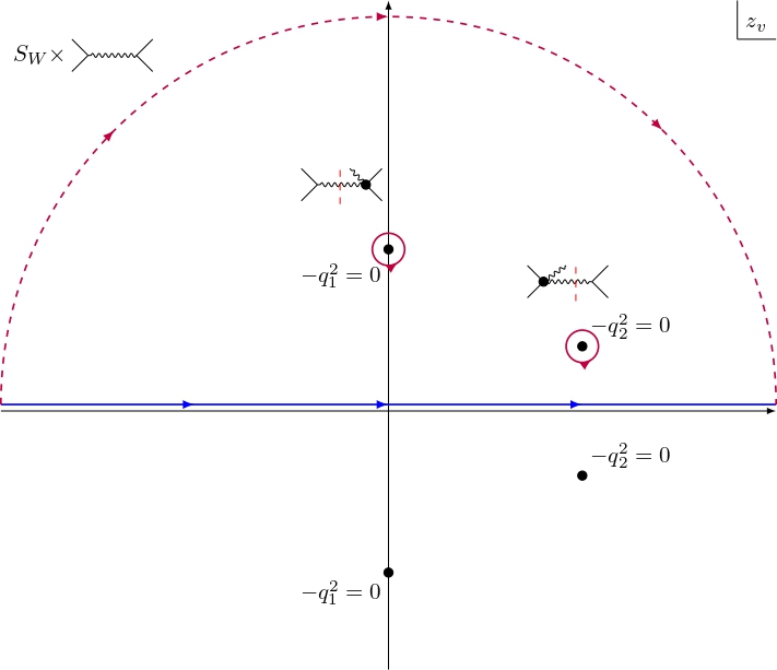
Figure 8: The deformation of the contour $\color[rgb]{1,0,0}{\mathcal{C}^{(+)}}$ in the complex $z_{v}$ plane allows to evaluate the integral of the five-point tree-level amplitude directly in terms of the factorization channels. Figure reproduced from Ref. [114].

Thanks to the Riemann-Lebesgue’s lemma it is possible to show that the principal value of the integral over the dotted half-circumference vanishes in the limit of infinite radius; hence, using the Cauchy theorem, we have

$$\int_{-\infty}^{+\infty}\mathrm{d}z_{v}\,\hat{\mathcal{M}}_{5,\rm cl}^{(0)}(q_{1},q_{2},k^{\lambda})=\int_{\color[rgb]{1,0,0}{\mathcal{C}^{(+)}}}\!\mathrm{d}z_{v}\,\hat{\mathcal{M}}_{5,\rm cl}^{(0)}(q_{1},q_{2},k^{\lambda})\equiv I^{\lambda}_{\text{UHP}}$$ (8.19)

$$\hskip 71.13188pt\Rightarrow I^{\lambda}_{\text{UHP}}=2\pi i\sum_{i}\mathop{\mathrm{Res}}_{z=z_{i}}\hat{\mathcal{M}}_{5,\rm cl}^{(0)}(q_{1},q_{2},k^{\lambda})$$

Let us now study the poles of this integrand.

We have simple poles of the tree-level five-point amplitude in the complex $z_{v}$-plane corresponding to $q_{1}^{2}=0$ and $q_{2}^{2}=0$ which correspond to factorization channels:

$$\begin{split}\frac{I_{\mathcal{C}^{(+)}_{q_{1}}}^{\lambda}}{2\pi i}&=\sum_{h}\mathcal{M}_{4,\mathrm{cl}}^{(0)}(p_{2},k^{\lambda},-q_{1}^{h})\mathcal{M}_{3,\mathrm{cl}}^{(0)}(p_{1},q_{1}^{h})\operatornamewithlimits{Res}_{z=\hat{z}_{1}}\frac{-1}{q_{1}^{2}}\,,\\ \frac{I_{\mathcal{C}^{(+)}_{q_{2}}}^{\lambda}}{2\pi i}&=\sum_{h}\mathcal{M}_{4,\mathrm{cl}}^{(0)}(p_{1},k^{\lambda},-q_{2}^{h})\mathcal{M}_{3,\mathrm{cl}}^{(0)}(p_{2},q_{2}^{h})\operatornamewithlimits{Res}_{z=\hat{z}_{2}}\frac{-1}{q_{2}^{2}}\,,\end{split}$$ (8.20)

where $\hat{z}_{1}$ and $\hat{z}_{2}$ are the solutions in the UHP of the pole constraints $-q_{i}^{2}=0$.
The pole(s) $\hat{z}_{1}$ are given by the solutions of

$$-q_{1}^{2}=-(z_{1}^{2}+z_{2}^{2}+2\gamma z_{1}z_{2}-z_{v}^{2}-z_{b}^{2})=0\,,$$ (8.21)

recalling now that in the hatted-kinematics

$$z_{1}=\dfrac{\gamma}{\gamma^{2}-1}\omega_{2}\,,\qquad z_{2}=-\dfrac{1}{\gamma^{2}-1}\omega_{2}\,,$$ (8.22)

we find

$$-q_{1}^{2}=z_{v}^{2}+z_{b}^{2}+\omega_{2,r}^{2}=(z_{v}-\hat{z}_{1})(z_{v}-\hat{z}_{1}^{*})=0\,,$$ (8.23)

with

$$\hat{z}_{1}=i\sqrt{z_{b}^{2}+w_{2,r}^{2}}\,.$$ (8.24)

Meanwhile, the pole(s) $\hat{z}_{2}$ are given by the solutions of

$$-q_{2}^{2} =-(k-q_{1})^{2}=-q_{1}^{2}+2k\cdot q_{1}=$$ (8.25)

$$=-(z_{1}^{2}+z_{2}^{2}+2\gamma z_{1}z_{2}-z_{v}^{2}-z_{b}^{2})+2z_{1}(k\cdot v_{1})+2z_{2}(k\cdot v_{2})+2z_{v}(k\cdot\tilde{v})+2z_{b}(k\cdot\tilde{b})=0\,,$$

which, after imposing the constraints in Eq. (8.22), becomes

$$-q_{2}^{2} =z_{v}^{2}+z_{b}^{2}+\omega_{2,r}^{2}+2\gamma\omega_{1,r}\omega_{2,r}-2\omega_{2,r}^{2}+2z_{v}(k\cdot\tilde{v})+2z_{b}(k\cdot\tilde{b})=$$

$$=(z_{v}+k\cdot\tilde{v})^{2}+(z_{b}+k\cdot\tilde{b})^{2}-(k\cdot\tilde{v})^{2}-(k\cdot\tilde{b})^{2}-\omega_{2,r}^{2}+2\gamma\omega_{1,r}\omega_{2,r}\,.$$ (8.26)

Notice now that

$$-(k\cdot\tilde{v})^{2}=(k\cdot\tilde{b})^{2}+\omega_{1,r}^{2}+\omega_{2,r}^{2}-2\gamma\omega_{1,r}\omega_{2,r}\,,$$ (8.27)

henceforth Eq. (8) reduces to

$$-q_{2}^{2} =(z_{v}+k\cdot\tilde{v})^{2}+(z_{b}+k\cdot\tilde{b})^{2}+\omega_{1,r}^{2}=(z_{v}-\hat{z}_{2})(z_{v}-\hat{z}_{2}^{*})=0\,,$$ (8.28)

with

$$\hat{z}_{2}=-\tilde{v}\cdot k+i\sqrt{(z_{b}+\tilde{b}\cdot k)^{2}+w_{1,r}^{2}}\,,$$ (8.29)

Other than the residues related to these simple poles, we should also take into account (half) the residue at infinity of the five-point amplitude, which we label as $I_{\mathcal{C}^{(+)}_{\infty}}^{\lambda}$ .

Summarizing, we have the following equality

$$I_{\text{UHP}}^{\lambda}=I^{\lambda}_{\mathcal{C}^{(+)}_{q_{1}}}+I^{\lambda}_{\mathcal{C}^{(+)}_{q_{2}}}+I^{\lambda}_{\mathcal{C}^{(+)}_{\infty}}\,,$$ (8.30)

The treatment of the residue at infinity is quite delicate, as it can have spurious pole that cancel only at later stages. To avoid having to deal with this problem we can use the following trick: we split the $z_{v}$-integration into two equal pieces and deform the integration contour in the UHP and LHP. As a consequence, the contributions from the arcs at infinity cancel each other ($I^{\lambda}_{\mathcal{C}^{(+)}_{\infty}}=I^{\lambda}_{\mathcal{C}^{(-)}_{\infty}}$) and only the finite poles contribute:

$$\int_{-\infty}^{+\infty}\mathrm{d}z_{v}\ \hat{\mathcal{M}}_{5,\rm cl}^{(0)} =\frac{1}{2}\left(I_{\text{UHP}}^{\lambda}-I_{\text{LHP}}^{\lambda}\right)=\frac{1}{2}\left(I^{\lambda}_{\mathcal{C}^{(+)}_{q_{1}}}+I^{\lambda}_{\mathcal{C}^{(+)}_{q_{2}}}-I^{\lambda}_{\mathcal{C}^{(-)}_{q_{1}}}-I^{\lambda}_{\mathcal{C}^{(-)}_{q_{2}}}\right)$$

$$=i\pi\sum_{i=1,2}\left(\underset{z_{v}=z_{i}}{Res}\hat{\mathcal{M}}_{5,\rm cl}^{(0)}-\underset{z_{v}=z_{i}^{*}}{Res}\hat{\mathcal{M}}_{5,\rm cl}^{(0)}\right)\,.$$ (8.31)

The direct computation of the $z_{b}$ integral is rather involved and evaluates to Bessel functions, as shown in Ref. [116] and Ref. [117]; however, since we are interested in the strain at future null infinity we need to compute the waveform in the time domain. By switching the order of integration, the computation greatly simplifies.
To compute the $\omega$ integral, it is useful to extract all $\omega$ dependencies and define the dimensionless variables

$$w_{i}\to\omega\,\bar{w}_{i}\ ,\,\,\,\bar{w}_{i}=n\cdot v_{i}\,,\quad z_{v}\to\omega\,z_{v}\,,\quad z_{b}\to\omega\,z_{b}\,.$$ (8.32)

To determine the scaling of $\hat{\mathcal{M}}^{(0)}_{5,\rm cl}$ with $\omega$, notice that the five-point amplitude has dimension $4-5=-1$, however the gravitational coupling $\kappa$ has dimension $-1$ and in the perturbative expansion we have $\hat{\mathcal{M}}^{(L)}_{5,\rm cl}\sim\kappa^{3+2L}$. Notice that if we express the Mandelstam variables of $\hat{\mathcal{M}}^{(0)}_{5,\rm cl}(q_{1},q_{2},k)$ using Eq. (8.32), the only dimensionful parameter is $\omega$. Indeed

$$\begin{gathered}-q_{1}^{2}=\omega^{2}(z_{v}^{2}+z_{b}^{2}+\bar{\omega}^{2}_{2,r})\,,\qquad-q_{2}^{2}=\omega^{2}\left[(z_{v}+n\cdot\tilde{v})^{2}+(z_{b}+n\cdot\tilde{b})^{2}+\bar{\omega}^{2}_{1,r}\right]\,,\\ k^{2}=0\,,\qquad k\cdot q_{1}=\omega\bar{\omega}_{1}\,,\qquad k\cdot q_{2}=\omega\bar{\omega}_{2}\,.\end{gathered}$$ (8.33)

If we now express $\hat{\mathcal{M}}^{(0)}_{5,\rm cl}(q_{1},q_{2},k)$ as

$$\hat{\mathcal{M}}^{(0)}_{5,\rm cl}(q_{1},q_{2},k)=\kappa^{3}\omega^{\alpha}f(\bar{\omega}_{i},z_{v},z_{b})\,.$$ (8.34)

Since $\omega$ has dimension $1$, by dimensional analysis we find the $\omega$ dependence of this amplitude to be fixed by

$$[\mathcal{M}_{5,{\rm cl}}^{(0)}]=[\kappa^{3}][\omega^{\alpha}]\quad\Rightarrow\quad-1=-3+\alpha\,.$$ (8.35)

Since $\omega$ has dimension $1$, we finally obtain $\alpha=2$. Therefore to extract all $\omega$ dependencies out of $\mathcal{M}_{5,\rm cl}^{(0)}$ we rescale it as

$$\mathcal{M}_{5,\rm cl}^{(0)}\to\omega^{-2}\mathcal{M}_{5,{\rm cl}}^{(0)}\,.$$ (8.36)

Using now the fact that, at tree level,

$$W^{(0)}(b,k^{\pm})=[W^{(0)}(-b,k^{\mp})]^{*}\,,$$ (8.37)

we are finally able to rewrite Eq. (8.1) as:

$$h^{(0)}(x)= \frac{\kappa}{8\pi|\vec{x}\,|}\int_{-\infty}^{\infty}\!\hat{\mathrm{d}}\omega\ \Big{[}W^{(0)}(b;k^{-})e^{-i\omega u}\Big{]}=$$

$$=\frac{\kappa}{8\pi|\vec{x}\,|}\int_{-\infty}^{\infty}\!\hat{\mathrm{d}}\omega\ \left[\int\!\mathrm{d}z_{v}\mathrm{d}z_{b}\,e^{-iz_{b}\sqrt{-b^{2}}}\frac{\hat{\mathcal{M}}_{5,\rm cl}^{(0)}}{(4\pi)^{2}m_{1}m_{2}\sqrt{\gamma^{2}-1}}e^{-i\omega u}\right]=$$

$$=\frac{\kappa}{8\pi|\vec{x}\,|}\int_{-\infty}^{\infty}\!\hat{\mathrm{d}}\omega\ \left[\int\!\mathrm{d}z_{v}\mathrm{d}z_{b}\,\omega^{2}\,e^{-i\omega\,z_{b}\sqrt{-b^{2}}}\frac{\omega^{-2}\,\hat{\mathcal{M}}_{5,\rm cl}^{(0)}}{(4\pi)^{2}m_{1}m_{2}\sqrt{\gamma^{2}-1}}e^{-i\omega u}\right]=$$

$$=\frac{\kappa}{8\pi|\vec{x}\,|}\int_{-\infty}^{\infty}\!\hat{\mathrm{d}}\omega\ \left[\int\!\mathrm{d}z_{b}\,e^{-i\omega\,z_{b}\sqrt{-b^{2}}}\frac{\left(I_{\text{UHP}}^{\lambda}-I_{\text{LHP}}^{\lambda}\right)}{2(4\pi)^{2}m_{1}m_{2}\sqrt{\gamma^{2}-1}}e^{-i\omega u}\right]=$$

$$=\frac{\kappa}{8\pi|\vec{x}\,|}\int\!\mathrm{d}z_{b}\frac{\left(I_{\text{UHP}}^{\lambda}-I_{\text{LHP}}^{\lambda}\right)}{2(4\pi)^{2}m_{1}m_{2}\sqrt{\gamma^{2}-1}}\int_{-\infty}^{\infty}\!\hat{\mathrm{d}}\omega\,e^{-i\omega\,(z_{b}\sqrt{-b^{2}}+u)}=$$

$$=\frac{\kappa}{8\pi|\vec{x}\,|}\int\!\mathrm{d}z_{b}\frac{\left(I_{\text{UHP}}^{\lambda}-I_{\text{LHP}}^{\lambda}\right)}{2(4\pi)^{2}m_{1}m_{2}\sqrt{\gamma^{2}-1}}\delta(z_{b}\sqrt{-b^{2}}+u)$$ (8.38)

Therefore, we have

$$h^{(0)}(x)=\frac{\kappa}{(4\pi)^{3}|\vec{x}|\sqrt{-b^{2}}}\frac{(I_{\text{UHP}}^{\lambda}-I_{\text{LHP}}^{\lambda})}{4m_{1}m_{2}\sqrt{\gamma^{2}-1}}\Bigg{|}_{z_{b}=-u/\sqrt{-b^{2}}}\,,$$ (8.39)

From this point onwards a direct computation becomes rather involved, therefore I will resort to Mathematica to obtain the final result.

8.1 Tree-level waveform for Schwarzschild black holes

We now compute the tree-level scattering waveform for spinless particles by combining Eq. (8.39), Eq. (8.20) and Eq. (8) with the three-point and four-point amplitudes previously obtained:

$$\mathcal{M}_{3,\rm cl}^{(0)}(p,k) =-\kappa\,m^{2}(\varepsilon\cdot v)^{2}\,,$$

$$\mathcal{M}_{4,\text{cl}}^{(0)}(p,k_{1},k_{2}) =\frac{\kappa^{2}m^{2}}{q^{2}}\left(\frac{v\cdot F_{1}\cdot F_{2}\cdot v}{v\cdot k_{1}}\right)^{2}\,,$$ (8.40)

with $q=(q_{1}-q_{2})/2$.

Substituting in Eq. (8.39), we find

$$\begin{split}&h^{(0)}(x)=\frac{G^{2}m_{1}m_{2}}{|\vec{x}\,|\sqrt{-b^{2}}}\frac{1}{\bar{w}_{1}^{2}\bar{w}_{2}^{2}\sqrt{1+T_{2}^{2}}\left(\gamma+\sqrt{\left(1+T_{1}^{2}\right)\left(1+T_{2}^{2}\right)}+T_{1}T_{2}\right)}\\ &\quad\times\Bigg{(}\frac{3\bar{w}_{1}+2\gamma\left(2T_{1}T_{2}\bar{w}_{1}-T_{2}^{2}\bar{w}_{2}+\bar{w}_{2}\right)-\left(2\gamma^{2}-1\right)\bar{w}_{1}}{\gamma^{2}-1}f_{1,2}^{2}\\ &\quad-\frac{4\gamma T_{2}\bar{w}_{2}f_{1}+2\left(2\gamma^{2}-1\right)\left[T_{1}\left(1+T_{2}^{2}\right)\bar{w}_{2}f_{1}+T_{2}(T_{1}T_{2}\bar{w}_{1}+\bar{w}_{2})f_{2}\right]}{\sqrt{\gamma^{2}-1}}f_{1,2}\\ &\quad+4\left(1+T_{2}^{2}\right)\bar{w}_{2}f_{1}f_{2}-4\gamma\left(1+T_{2}^{2}\right)\bar{w}_{2}\left(f_{1}^{2}+f_{2}^{2}\right)+2\left(2\gamma^{2}-1\right)\left(1+2T_{2}^{2}\right)\bar{w}_{2}f_{1}f_{2}\Bigg{)}+\left(1\leftrightarrow 2\right)\ ,\end{split}$$ (8.41)

where we have defined

$$T_{i} \coloneq\frac{\sqrt{\gamma^{2}-1}\,(u-b_{i}\cdot n)}{\sqrt{-(b_{1}-b_{2})^{2}}\,\bar{w}_{i}}\ ,$$ (8.42)

$$S^{2} \coloneq\frac{T_{1}^{2}-2\gamma T_{1}T_{2}+T_{2}^{2}}{\gamma^{2}-1}-1\ ,$$ (8.43)

$$f_{1,2} =v_{1}\cdot\varepsilon_{k}\,v_{2}\cdot n-v_{1}\cdot n\,v_{2}\cdot\varepsilon_{k}\ ,$$ (8.44)

$$f_{i} =\tilde{b}\cdot\varepsilon_{k}\,v_{i}\cdot n-\tilde{b}\cdot n\,v_{i}\cdot\varepsilon_{k}\ .$$ (8.45)

8.2 Tree-level waveform for Kerr black holes

Let us now compute tree-level scattering waveform Kerr black holes, that we identify with spinning point particles. In this case the three-point and the four-point Compton amplitudes are:

$$\begin{gathered}\mathcal{M}^{(0)}_{3,\rm cl}=-\kappa\,m^{2}\,(\varepsilon\cdot v)^{2}\,\exp\left(\frac{i\,\varepsilon\cdot S\cdot k}{\varepsilon\cdot v}\right)\ ,\\ \mathcal{M}^{(0)}_{4,\rm cl}=\frac{\kappa^{2}m^{2}\omega_{0}^{2}}{8(k_{1}\cdot k_{2})(k_{1}\cdot v)^{2}}\exp\left(\frac{\omega_{1}}{\omega_{0}}\right)+\mathcal{O}(S^{5})\,,\end{gathered}$$ (8.46)

with

$$\begin{gathered}\omega_{0}=-2\,v\cdot F_{1}\cdot F_{2}\cdot v\,,\\ i\,\omega_{1}=k_{1}\cdot F_{2}\cdot v\,S\cdot F_{1}-\frac{(k_{1}-k_{2})\cdot v}{2}S\cdot F_{1}\cdot F_{2}+\left(1\leftrightarrow 2\right)\,,\end{gathered}$$ (8.47)

where $S$ is the (mass-normalized) spin tensor of the Kerr black holes and we have defined $A\cdot B\cdot C=A^{\mu\nu}B_{\nu\rho}C^{\rho\sigma}\eta_{\sigma\mu}$ and $A\cdot B=A^{\mu\nu}B_{\nu\mu}$.
Note that

$$\dfrac{\omega_{2}}{\omega_{0}}=\dfrac{1}{2}\left(\dfrac{\omega_{1}}{\omega_{0}}\right)^{2}\,,$$ (8.48)

where

$$\omega_{2} =(k_{1}\cdot k_{2})\bigg{[}S\cdot S\left(\frac{F_{1}\cdot F_{2}}{2}-v\cdot F_{1}\cdot F_{2}\cdot v\right)-2\,S\cdot S\cdot F_{1}\cdot F_{2}\bigg{]}$$

$$\qquad\qquad-\frac{\omega_{0}}{2}(k_{1}+k_{2})\cdot S\cdot S\cdot(k_{1}+k_{2})\ ,$$ (8.49)

and $A\cdot B\cdot C\cdot D=A^{\mu\nu}B_{\nu\rho}C^{\rho\sigma}D_{\sigma\mu}$. Hence, we can write, as anticipated in Sec. 6, the Compton amplitude up to fifth order in the spin tensor without any spurious pole as

$$\mathcal{M}^{(0)}_{4,\rm cl}=\kappa^{2}m^{2}\frac{\omega_{0}^{2}+\omega_{0}\omega_{1}+\omega_{0}\omega_{2}+\frac{1}{3}\omega_{1}\omega_{2}+\frac{1}{6}\omega_{2}^{2}}{8(k_{1}\cdot k_{2})(k_{1}\cdot v)^{2}}+\mathcal{O}(S^{5})\,.$$ (8.50)

We may now be tempted to directly substitute in Eq. (8.39) in order to compute the waveform up to the fourth order in spin for both black holes, i.e. $\mathcal{O}(S_{1}^{4},S_{2}^{4})$. However in this case the discussion is more delicate. Indeed, after applying the rescaling Eq. (8.32), the degree of homogeneity in $\omega$ is not the one predicted in Eq. (8.36), as the mass-dimension of $S_{i}^{\mu\nu}$ is $-1$. If we write the five-point amplitude in the spin-multipole expansion

$$\mathcal{M}^{(L)}_{5,{\rm cl}} =\sum_{s_{1},s_{2}=1}^{\infty}\left[S_{1}^{\mu_{1}\nu_{1}}\dots S_{1}^{\mu_{s_{1}}\nu_{s_{1}}}\right]\left[S_{2}^{\rho_{1}\sigma_{1}}\dots S_{2}^{\rho_{s_{2}}\sigma_{s_{2}}}\right]\mathcal{M}^{(L),(s_{1},s_{2})}_{\mu_{1}\nu_{1},\dots\mu_{s_{1}}\nu_{s_{1}},\rho_{1}\sigma_{1},\dots\rho_{s_{2}}\sigma_{s_{2}}}\ ,$$ (8.51)

the scaling will be

$$\mathcal{M}^{(L),(s_{1},s_{2})}\rightarrow\omega^{-2+L+s_{1}+s_{2}}\mathcal{M}^{(L),(s_{1},s_{2})}\,.$$ (8.52)

Therefore it is convenient to compute the tree-level five-point spinning waveform order by order in its spin-multipole expansion,i.e. 

$$h^{(0)}(x)=\sum_{s_{1},s_{2}=0}^{\infty}h^{(s_{1},s_{2})}(x)\,.$$ (8.53)

Let us now study how the $z_{v}$ integral gets modified.

$$h^{(s_{1},s_{2})}(x) =\frac{\kappa}{8\pi|\vec{x}\,|}\int_{-\infty}^{\infty}\!\hat{\mathrm{d}}\omega\ \left[\int\!\mathrm{d}z_{v}\mathrm{d}z_{b}\,e^{-iz_{b}\sqrt{-b^{2}}}\frac{\hat{\mathcal{M}}_{5,\rm cl}^{(0),(s_{1},s_{2})}}{(4\pi)^{2}m_{1}m_{2}\sqrt{\gamma^{2}-1}}e^{-i\omega u}\right]=$$ (8.54)

$$=\frac{\kappa}{8\pi|\vec{x}\,|}\int_{-\infty}^{\infty}\!\hat{\mathrm{d}}\omega\,\left[\int\!\mathrm{d}z_{v}\mathrm{d}z_{b}\,\omega^{2}\,e^{-i\omega\,z_{b}\sqrt{-b^{2}}}\frac{{\omega^{-2+s_{1}+s_{2}}\,\hat{\mathcal{M}}}_{5,\rm cl}^{(0)(s_{1},s_{2})}}{(4\pi)^{2}m_{1}m_{2}\sqrt{\gamma^{2}-1}}e^{-i\omega u}\right]=$$

$$=\frac{\kappa}{8\pi|\vec{x}\,|}\int\!\mathrm{d}z_{v}\mathrm{d}z_{b}\,\dfrac{\hat{\mathcal{M}}_{5,\rm cl}^{(0)(s_{1},s_{2})}}{(4\pi)^{2}m_{1}m_{2}\sqrt{\gamma^{2}-1}}\int_{-\infty}^{\infty}\!\hat{\mathrm{d}}\omega\,\omega^{s_{1}+s_{2}}e^{-i\omega(u+z_{b}\sqrt{-b^{2}}})=$$

$$=\frac{\kappa}{8\pi|\vec{x}\,|}\int\!\mathrm{d}z_{v}\mathrm{d}z_{b}\,\dfrac{\hat{\mathcal{M}}_{5,\rm cl}^{(0)(s_{1},s_{2})}}{(4\pi)^{2}m_{1}m_{2}\sqrt{\gamma^{2}-1}}\times$$

$$\hskip 85.35826pt\times\left(\dfrac{i}{\sqrt{-b^{2}}}\right)^{s_{1}+s_{2}}\frac{\partial^{(s_{1}+s_{2})}}{\partial z_{b}^{s_{1}+s_{2}}}\int_{-\infty}^{\infty}\!\hat{\mathrm{d}}\omega\,e^{-i\omega(u+z_{b}\sqrt{-b^{2}}})=$$

$$=\frac{\kappa}{8\pi|\vec{x}\,|}\left(\dfrac{i}{\sqrt{-b^{2}}}\right)^{s_{1}+s_{2}}\!\!\int\!\mathrm{d}z_{v}\mathrm{d}z_{b}\,\dfrac{\hat{\mathcal{M}}_{5,\rm cl}^{(0)(s_{1},s_{2})}}{(4\pi)^{2}m_{1}m_{2}\sqrt{\gamma^{2}-1}}\left(\frac{\partial^{(s_{1}+s_{2})}}{\partial z_{b}^{s_{1}+s_{2}}}\delta(u+z_{b}\sqrt{-b^{2}})\right)=$$

$$=\frac{\kappa}{2|\vec{x}\,|(4\pi)^{3}m_{1}m_{2}\sqrt{\gamma^{2}-1}}\dfrac{(-i)^{s_{1}+s_{2}}}{(\sqrt{-b^{2}})^{s_{1}+s_{2}}}\times$$

$$\hskip 85.35826pt\times\int\!\mathrm{d}z_{v}\mathrm{d}z_{b}\,\delta(u+z_{b}\sqrt{-b^{2}})\left(\frac{\partial^{(s_{1}+s_{2})}}{\partial z_{b}^{s_{1}+s_{2}}}\hat{\mathcal{M}}_{5,\rm cl}^{(0)(s_{1},s_{2})}\right)=$$

$$=\frac{\kappa}{2|\vec{x}\,|(4\pi)^{3}m_{1}m_{2}\sqrt{\gamma^{2}-1}}\dfrac{(-i)^{s_{1}+s_{2}}}{(\sqrt{-b^{2}})^{s_{1}+s_{2}+1}}\frac{\partial^{(s_{1}+s_{2})}}{\partial z_{b}^{s_{1}+s_{2}}}\int\!\mathrm{d}z_{v}\,\hat{\mathcal{M}}_{5,\rm cl}^{(0)(s_{1},s_{2})}\Bigg{|}_{z_{b}=-u/\sqrt{-b^{2}}}$$

Consequently, the spinning tree-level waveform can be computed order by order, isolating the $s_{1}^{\rm th}$ and $s_{2}^{\rm th}$ multipoles in the factorized amplitudes, as

$$h^{(s_{1},s_{2})}(x)=\frac{\kappa}{(4\pi)^{3}\,|\vec{x}|\,(\sqrt{-b^{2}})^{s_{1}+s_{2}+1}}\frac{(-i)^{s_{1}+s_{2}}}{4m_{1}m_{2}\sqrt{\gamma^{2}-1}}\frac{\partial^{(s_{1}+s_{2})}}{\partial z_{b}^{s_{1}+s_{2}}}(I_{\text{UHP}}^{(s_{1},s_{2})}-I_{\text{LHP}}^{(s_{1},s_{2})})\Bigg{|}_{z_{b}=-u/\sqrt{-b^{2}}}\,.$$ (8.55)

In conclusion, we have

$$h^{(0)}(x)=\sum_{s_{1},s_{2}=0}^{4}\dfrac{G^{2}m_{1}m_{2}}{|\vec{x}|(\sqrt{-b^{2}})^{s_{1}+s_{2}+1}}\mathfrak{h}_{s_{1},s_{2}}(x)+\mathcal{O}(S_{1}^{5},S_{2}^{5})\,,$$ (8.56)

where the $\mathfrak{h}_{s_{1},s_{2}}$’s are provided in the ancillary files obtained in Ref. [114].

9 Conclusions

In this thesis, I have studied the classical scattering problem of two Kerr black holes in general relativity using novel quantum field theory techniques within the Post-Minkowskian expansion, extending the subleading soft theorem to account for spinning particles.
I began by describing the spinor-helicity formalism, which served as a foundational tool for computing basic amplitudes. I then introduced a general method for obtaining higher-point amplitudes, utilizing the BCFW recursion relations to compute them in a general context. This was later refined to the soft recursion relations, which I applied to compute $(n+1)$-point amplitudes involving one additional external graviton, starting from the corresponding $n$-point amplitudes.
With these tools in place, I computed the gravitational Compton amplitude for both spinless and spinning black holes, and the elastic 2-to-2 black hole scattering amplitudes. I also derived the five-point amplitude, which represents the first original result in this thesis. While the five-point amplitude exists in the literature, to my knowledge, no prior work has computed it using soft recursion on the four-point amplitude.

In parallel, I emphasized the necessity of a classical formulation for scattering amplitudes and introduced the KMOC formalism, detailing its complexities and offering a general method for computing observables. In this context, I re-evaluated all quantum amplitudes to derive their classical counterparts, presenting a straightforward method for calculating the classical (infinite-spin) limit.
Additionally, I introduced a classical version of the soft recursion relations to derive higher-point classical amplitudes from lower-point ones in a purely classical setting—an approach that, to my knowledge, is presented here for the first time.

Finally, I applied the KMOC formalism to compute the leading-order waveform for black hole scattering with radiation emission, covering both the spinning and spinless cases.

There are several compelling future directions that can be explored:

• Investigating the structure of spurious poles starting from the $\mathcal{O}(S^{4})$ term in the Compton amplitude for spinning particles could provide new insights into the dynamics of spinning black holes.

• A deeper understanding of the higher orders in the five-point amplitude, especially in connection with effects like the Spin Memory Effect, could pave the way for more accurate calculations of spin-related phenomena in classical black hole scattering.

• Further exploration of the relationship between soft factors and asymptotic symmetries is another promising avenue.

• It would also be valuable to investigate the double copy structure of soft theorems for massive particles.

• Finally, it wold be interesting to extend these results to higher-loop or PM orders, including radiative corrections and finite-size effects.

10 Acknowledgements

I would like to express my heartfelt gratitude to Prof. Vittorio Del Duca for guiding and supporting me during this journey. A sincere thank you to Dr. Riccardo Gonzo, my thesis co-advisor, for his immense patience, invaluable advice, and the knowledge they imparted throughout the entire process of writing this thesis.
I am also deeply grateful to the professors at Sapienza, whose teachings sparked my passion for theoretical physics, without whom I would not have reached this milestone.
To my family, friends, and university colleagues, thank you for making this achievement truly special.

Appendix A Conventions

A.1 Lorentz algebra

I follow the work discussed in chapter 27 of Ref. [118], and in particular I will mostly follow the notation presented in Ref. [99].
We work with the metric $\eta_{\mu\nu}=\text{diag}(+1,-1,-1,-1)$, so that $p^{2}=p^{\mu}p_{\mu}=(p_{0})^{2}-(\vec{p})^{2}$. Our convention for the Lorentz generators are fixed by the algebra,

$$\left[J^{\mu\nu},J^{\lambda\sigma}\right]=-i\left(\eta^{\mu\lambda}J^{\nu\sigma}+\eta^{\nu\sigma}J^{\mu\lambda}-\eta^{\mu\sigma}J^{\nu\lambda}-\eta^{\nu\lambda}J^{\mu\sigma}\right)\,.$$ (A.1)

To relate the (connected part) of the Lorentz group $SO(1,3)$ and its double cover $SL(2,\mathbb{C})$, we follow a widely adopted convention for spinors and gamma matrices,

$$\gamma^{\mu}=\begin{pmatrix}0&(\sigma^{\mu})_{\alpha\dot{\beta}}\\ (\bar{\sigma}^{\mu})^{\dot{\alpha}\beta}&0\end{pmatrix}\,,\quad\sigma^{\mu}=({\hbox to0.0pt{1\hss}\hskip 1.6pt\hbox{1}},\vec{\sigma})\,,\quad\bar{\sigma}^{\mu}=({\hbox to0.0pt{1\hss}\hskip 1.6pt\hbox{1}},-\vec{\sigma})\,,$$ (A.2)

where $\vec{\sigma}$ denote Pauli matrices. Complex conjugation exchanges undotted and dotted indices. Spinor indices are raised and lowered by the invariant tensor of $SL(2,\mathbb{C})$ satisfying

$$\epsilon_{\alpha\beta}=-\epsilon_{\beta\alpha}\,,\quad\epsilon_{\alpha\beta}\epsilon^{\beta\gamma}=\delta_{\alpha}{}^{\gamma}\,,\quad\epsilon^{12}=+1\,,\quad\epsilon_{\dot{\alpha}\dot{\beta}}=(\epsilon_{\alpha\beta})^{*}\,.$$ (A.3)

For example, $\lambda^{\alpha}=\epsilon^{\alpha\beta}\lambda_{\beta}$ and $\tilde{\lambda}_{\dot{\alpha}}=\epsilon_{\dot{\alpha}\dot{\beta}}\tilde{\lambda}^{\dot{\beta}}$.

For any (momentum) 4-vector, the bi-spinor notation is defined by

$$p_{\alpha\dot{\alpha}}=p_{\mu}(\sigma^{\mu})_{\alpha\dot{\alpha}}\,,\quad p^{2}=\det(p_{\alpha\dot{\alpha}})=\frac{1}{2}\epsilon^{\alpha\beta}\epsilon^{\dot{\alpha}\dot{\beta}}p_{\alpha\dot{\alpha}}p_{\beta\dot{\beta}}\,.$$ (A.4)

A.2 Massless momenta

For massless momenta, $p_{\alpha\dot{\alpha}}$ as a $(2\times 2)$ matrix has rank 1, so it can be written as

$$p_{\alpha\dot{\alpha}}=\lambda_{\alpha}\tilde{\lambda}_{\dot{\alpha}}\,.$$ (A.5)

For a real momentum, the spinors satisfy the reality condition,

$$(\lambda_{\alpha})^{*}=\text{sign}(p_{0})\tilde{\lambda}_{\dot{\alpha}}\,.$$ (A.6)

The Little group $U(1)$ acts on the spinors as

$$\lambda\rightarrow e^{-i\frac{\theta}{2}}\lambda\,,\quad\tilde{\lambda}\rightarrow e^{i\frac{\theta}{2}}\tilde{\lambda}\,.$$ (A.7)

The spinors for $p$ and those for $(-p)$ must be proportional. We fix the relation by setting

$$\lambda(-p)=i\lambda(p)\,,\quad\tilde{\lambda}(-p)=i\tilde{\lambda}(p)\,.$$ (A.8)

It is customary to introduce a bra-ket notation,

$$|p\rangle\leftrightarrow\lambda_{\alpha}\,,\quad\langle p|\leftrightarrow\lambda^{\alpha}\,,\quad|p]\leftrightarrow\tilde{\lambda}^{\dot{\alpha}}\,,\quad[p|\leftrightarrow\tilde{\lambda}_{\dot{\alpha}}\,,$$ (A.9)

which leads to the Lorentz invariant, Little group covariant brackets,

$$\langle ij\rangle=\lambda_{i}^{\alpha}\lambda_{j}^{\beta}\epsilon_{\alpha\beta}=\lambda_{i}^{\alpha}\lambda_{j\beta}\,,\quad[ij]=\tilde{\lambda}_{i\dot{\alpha}}\tilde{\lambda}_{j}^{\dot{\alpha}}\,.$$ (A.10)

The massless Mandelstam variables, which are both Lorentz invariant and Little group invariant, can be expressed as

$$2p_{i}\cdot p_{j}=\epsilon^{\alpha\beta}\epsilon^{\dot{\alpha}\dot{\beta}}(p_{i})_{\alpha\dot{\alpha}}(p_{j})_{\beta\dot{\beta}}=\langle ij\rangle[ji]\,.$$ (A.11)

A.3 Massive momenta

For massive momenta, the on-shell condition in the bi-spinor notation is given by

$$\det(p_{\alpha\dot{\alpha}})=m^{2}\,.$$ (A.12)

The massive helicity spinor variables are defined by

$$p_{\alpha\dot{\alpha}}=\lambda_{\alpha}{}^{I}\tilde{\lambda}_{I\dot{\alpha}}\,,\quad\det(\lambda_{\alpha}{}^{I})=m=\det(\tilde{\lambda}_{I\dot{\alpha}})\,.$$ (A.13)

The index $I$ indicates a doublet of the $SU(2)$ Little group. The reality condition reads

$$(\lambda_{\alpha}{}^{I})^{*} =\text{sign}(p_{0})\tilde{\lambda}_{I\dot{\alpha}}$$ (A.14)

$$(\lambda_{\alpha}{}_{I})^{*} =-\text{sign}(p_{0})\tilde{\lambda}^{I}_{\dot{\alpha}}\,.$$ (A.15)

SU(2)-invariant tensor

Given a matrix representation of the doublet of $SU(2)$,

$$\psi^{I}\rightarrow U^{I}{}_{J}\psi^{J}\,,$$ (A.16)

the two defining properties of $SU(2)$ can be written as

$$\epsilon_{IK}U^{I}{}_{J}U^{K}{}_{L}=\epsilon_{JL}\,,\quad U^{I}{}_{J}(U^{\dagger})^{J}{}_{K}=\delta^{I}{}_{K}\,,$$ (A.17)

where the $SU(2)$-invariant tensor $\epsilon_{IJ}$ shares, by convention, the first three properties in eq.(A.3). Just like spinor indices, the Little group indices are raised and lowered by $\epsilon_{IJ}$ and $\epsilon^{IJ}$. It follows from eq.(A.17) that the two variables below transform in the same way.

$$\psi_{I}\mathrel{\mathop{\mathchar 58\relax}}=\epsilon_{IJ}\psi^{J}\quad\mbox{and}\quad\bar{\psi}_{I}\mathrel{\mathop{\mathchar 58\relax}}=(\psi^{I})^{*}\,.$$ (A.18)

Then,

$$p_{\alpha\dot{\alpha}}=\lambda_{\alpha}{}^{I}\tilde{\lambda}_{I\dot{\alpha}}=-\lambda_{\alpha I}\tilde{\lambda}^{I}{}_{\dot{\alpha}}\,,\quad\bar{p}^{\dot{\alpha}\alpha}=p_{\mu}(\bar{\sigma}^{\mu})^{\dot{\alpha}\alpha}=\epsilon^{\dot{\alpha}\dot{\beta}}\epsilon^{\alpha\beta}p_{\beta\dot{\beta}}=\lambda^{\alpha I}\tilde{\lambda}_{I}{}^{\dot{\alpha}}=-\lambda^{\alpha}{}_{I}\tilde{\lambda}^{I\dot{\alpha}}\,.$$ (A.19)

It is also useful to note that

$$\epsilon^{\alpha\beta}\lambda_{\alpha}{}^{I}\lambda_{\beta}{}^{J}=\det(\lambda)\epsilon^{IJ}=m\epsilon^{IJ}\,,\quad\epsilon^{\dot{\alpha}\dot{\beta}}\tilde{\lambda}_{I\dot{\alpha}}\tilde{\lambda}_{J\dot{\beta}}=-\det(\tilde{\lambda}){\epsilon}_{IJ}=-m{\epsilon}_{IJ}\,.$$ (A.20)

Dirac spinors

By definition, the massive spinor helicity variables satisfy the Dirac equation

$$p_{\alpha\dot{\alpha}}\tilde{\lambda}^{\dot{\alpha}I}=m\lambda_{\alpha}{}^{I}\,,\quad p^{\dot{\alpha}\alpha}\lambda_{\alpha}{}^{I}=m\tilde{\lambda}^{\dot{\alpha}I}\,.$$ (A.21)

For a fixed massive particle, the $SU(2)$ Little group is always completely symmetrized. For convenience, we use the BOLD notation to suppresses the $SU(2)$ little group indices.

The Dirac equation eq.(A.21) can be written in the BOLD bra-ket notation as

$$p|\mathbf{p}]=m|\mathbf{p}\rangle\,,\quad\langle\mathbf{p}|p=-m[\mathbf{p}|\,.$$ (A.22)

As a final consistency check, it is important to see how these massive momenta behave in the high energy limit. This discussion is explained in detail in the appendix A.4 of Ref. [99]: massive momenta behave as massless ones, with corrections proportional to the quantity $m/E$. Note that those arguments become crucial when we study the UV behaviour of our theory.

Appendix B Spin tensor for spin-1 matter

I will now discuss the spin tensor for a massive spin-1 particle. The starting point is the one-particle expectation value of the angular-momentum operator in the quantum-
mechanical sense:

$$S_{p}^{\mu\nu}=\frac{\langle p|J^{\mu\nu}|p\rangle}{\langle p|p\rangle}=\frac{\varepsilon_{p,\sigma}^{*}J^{\mu\nu,\sigma}_{~{}~{}~{}~{}\;\tau}\epsilon_{p}^{\tau}}{\varepsilon_{p}^{*}\cdot\varepsilon_{p}}=2i\varepsilon_{p}^{*[\mu}\varepsilon_{p}^{\nu]}\,,\quad\text{where}\quad J^{\mu\nu,\sigma}_{~{}~{}~{}~{}~{}\tau}=i[\eta^{\mu\sigma}\delta^{\nu}_{\tau}-\eta^{\nu\sigma}\delta^{\mu}_{\tau}]\,,$$ (B.1)

where $J^{\mu\nu}$ are the Lorentz generators in the vector representation. Notica that, due to the transversality of the massive polarization vectors, we have $p_{\mu}S^{\mu\nu}=0$.
We are now interested in generalizing Eq. (B.1) to the case in which the two external states are different, in particular we will denote the incoming momentum as $p_{1}$ and the outgoing with $p_{2}$.

We may now introduce the notion of generalized expectation value (GEV) in the following way:

$$S_{12}^{\mu\nu}=\frac{\langle\mathbf{2}|J^{\mu\nu}|\mathbf{1}\rangle}{\langle\mathbf{2}|\mathbf{1}\rangle}=\frac{\varepsilon_{2\sigma}^{*}J^{\mu\nu,\sigma}_{~{}~{}~{}~{}\;\tau}\varepsilon_{1}^{\tau}}{\varepsilon_{2}^{*}\cdot\varepsilon_{1}}=\frac{2i\varepsilon_{2}^{*[\mu}\varepsilon_{1}^{\nu]}}{\varepsilon_{2}^{*}\cdot\varepsilon_{1}}.$$ (B.2)

Notice that, when computing amplitudes using the spinor-helicity methods, we often prefer to work with all momenta incoming. To compare results obtained using these different choices, we analytically continue our bi-spinors to negative energies using the conventions explained in App. (A) and suppress the conjugation sign, thus

$$S_{12}^{\mu\nu}=-2i\varepsilon_{1}^{[\mu}\varepsilon_{2}^{\nu]}/(\varepsilon_{1}\cdot\varepsilon_{2}),$$ (B.3)

We end this discussion with the following consideration: in a classical computation it is desirable to consider a spin tensor that satisfies the spin supplementary condition (SSC), i.e. $p_{\mu}S^{\mu\nu}=0$. However,

$$p_{\mu}S_{12}^{\mu\nu}=-\frac{i}{2}\frac{(k\cdot\varepsilon_{2})\varepsilon_{1}^{\nu}+(k\cdot\varepsilon_{1})\varepsilon_{2}^{\nu}}{\varepsilon_{1}\cdot\varepsilon_{2}}\neq 0,\quad\text{where $k=-p_{1}-p_{2}$ }$$ (B.4)

Yet, the spin tensor is intrinsically ambiguous, as the separation between the orbital and intrinsic pieces of the total angular momentum is relativistically frame-dependent. This ambiguity allows the spin tensor to be transformed as $S^{\mu\nu}\rightarrow S^{\mu\nu}+p^{[\mu}r^{\nu]}$, where the difference $p^{[\mu}r^{\nu]}$ for some vector $r^{\nu}$ accounts for the relative shift between $S^{\mu\nu}$ and $L^{\mu\nu}\sim p^{[\mu}\frac{\partial}{\partial p^{\nu]}}$. Adjusting $r^{\nu}$ to accommodate for the SSC, we finally obtain

$$S^{\mu\nu}=S_{12}^{\mu\nu}+\frac{2}{m^{2}}\,p_{\lambda}S_{12}^{\lambda[\mu}p^{\nu]}=-\frac{i}{\varepsilon_{1}\cdot\varepsilon_{2}}\bigg{\{}2\varepsilon_{1}^{[\mu}\varepsilon_{2}^{\nu]}-\frac{1}{m^{2}}p^{[\mu}\big{(}(k\cdot\varepsilon_{2})\varepsilon_{1}+(k\cdot\varepsilon_{1})\varepsilon_{2}\big{)}^{\nu]}\bigg{\}}\,.$$ (B.5)

Appendix C Angular-momentum operator

Let us delve into the details of the angular momentum operator in the spinor-helicity formalism. Consider the total angular momentum $J_{\mu\nu}=L_{\mu\nu}+S_{\mu\nu}$. The orbital-piece in momentum-space is

$$L_{\mu\nu}=2i\,p_{[\mu}\frac{\partial}{\partial p^{\nu]}}=p_{\sigma}\Sigma_{\mu\nu,~{}\tau}^{~{}~{}~{}\sigma}\frac{\partial}{\partial p_{\tau}}\,,$$ (C.1)

where $\Sigma^{\mu\nu}$ are the Lorentz generators (in vector representation they are simply $J^{\mu\nu}$).

I will focus on the massive case, for a more general treatment see the appendix C of Ref. [100]. Recall that the massive momenta is $p^{\mu}=\frac{1}{2}\langle p^{a}|\sigma^{\mu}|p_{a}]$. The angular-momentum operator in the space of massive spinors $\{\lambda_{\alpha}^{a},\tilde{\lambda}_{\dot{\beta}}^{b}\}$ is given by (see Ref. [119]):

$$J^{\mu\nu}=\bigg{[}\lambda^{\alpha a}\sigma_{~{}~{}~{}\alpha}^{\mu\nu,~{}\,\beta}\frac{\partial~{}}{\partial\lambda^{\beta a}}+\tilde{\lambda}_{\dot{\alpha}}^{\,a}\bar{\sigma}^{\mu\nu,\dot{\alpha}}_{~{}~{}~{}~{}\,\dot{\beta}}\frac{\partial~{}}{\partial\tilde{\lambda}_{\dot{\beta}}^{a}}\bigg{]}\,,$$ (C.2)

where the matrices

$$\sigma^{\mu\nu,~{}\beta}_{~{}~{}~{}\alpha}=\frac{i}{4}(\sigma^{\mu}_{\alpha\dot{\gamma}}\bar{\sigma}^{\nu,\dot{\gamma}\beta}-\sigma^{\nu}_{\alpha\dot{\gamma}}\bar{\sigma}^{\mu,\dot{\gamma}\beta})\,,\qquad\bar{\sigma}^{\mu\nu,\dot{\alpha}}_{~{}~{}~{}~{}\dot{\beta}}=\frac{i}{4}(\bar{\sigma}^{\mu,\dot{\alpha}\gamma}\sigma^{\nu}_{\gamma\dot{\beta}}-\bar{\sigma}^{\nu,\dot{\alpha}\gamma}\sigma^{\mu}_{\gamma\dot{\beta}})\,,$$ (C.3)

are the left-handed and right-handed representations of the Lorentz-group algebra. Equivalently, we may express Eq. (C.2) in spinor indices as

$$J_{\alpha\dot{\alpha},\beta\dot{\beta}}=\sigma^{\mu}_{\alpha\dot{\alpha}}\sigma^{\nu}_{\beta\dot{\beta}}J_{\mu\nu}=2i\bigg{[}\lambda_{(\alpha}^{~{}a}\frac{\partial}{\partial\lambda^{\beta)a}}\epsilon_{\dot{\alpha}\dot{\beta}}+\epsilon_{\alpha\beta}\tilde{\lambda}_{(\dot{\alpha}}^{~{}a}\frac{\partial}{\partial\tilde{\lambda}^{\dot{\beta})a}}\bigg{]}\,.$$ (C.4)

Notice that this operator is by construction invariant under the little group ${\rm SU}(2)$.

We are now ready to discuss the action of the aforementioned angular momentum operator on massive spin-$s$ tensors. The (integer) spin-$s$ tensors are parametrized in terms of massive spinor-helicity variables as

$$\varepsilon_{\alpha_{1}\dot{\alpha}_{1}\dots\alpha_{s}\dot{\alpha}_{s}}^{a_{1}\dots a_{2s}}=\frac{2^{s/2}}{m^{s}}\lambda_{\alpha_{1}}^{(a_{1}}\lambda_{\dot{\alpha}_{1}}^{a_{2}}\cdots\lambda_{\alpha_{s}}^{a_{2s-1}}\lambda_{\dot{\alpha}_{s}}^{a_{2s})}.$$ (C.5)

Since $J^{\mu\nu}$ is a first-order differential operator, it distributes when acting on $\varepsilon^{a_{1}\cdots a_{2s}}$ according to the standard product rule for derivatives, i.e. 

$$J^{\mu\nu}\epsilon_{\alpha_{1}\dot{\alpha}_{1}\dots\alpha_{s}\dot{\alpha}_{s}}^{a_{1}\dots a_{2s}}=\frac{2^{s/2}}{m^{s}}\bigg{\{}\Big{[}\epsilon_{\alpha_{1}\beta}\big{(}\lambda^{\alpha(a_{1}}\sigma_{~{}~{}~{}\alpha}^{\mu\nu,~{}\,\beta}\big{)}\Big{]}\lambda_{\dot{\alpha}_{1}}^{a_{2}} \cdots\lambda_{\alpha_{s}}^{a_{2s-1}}\tilde{\lambda}_{\dot{\alpha}_{s}}^{a_{2s})}\,+$$

$$+\,\lambda_{\alpha_{1}}^{(a_{1}}\Big{[}\tilde{\lambda}_{\dot{\alpha}}^{a_{2}}\bar{\sigma}^{\mu\nu,\dot{\alpha}}_{~{}~{}~{}~{}\,\dot{\alpha_{2}}}\Big{]} \cdots\lambda_{\alpha_{s}}^{a_{2s-1}}\tilde{\lambda}_{\dot{\alpha}_{s}}^{a_{2s})}+\dots\bigg{\}}\,.$$ (C.6)

Finally, we remark that the action of the differential operator Eq. (C.4) is precisely that of the algebraic generator $\Sigma_{\mu\nu}$, indeed:

$$L_{\mu\nu}p^{\rho}=-\Sigma_{\mu\nu,~{}\sigma}^{~{}~{}~{}\rho}p^{\sigma}\,,\qquad(\varepsilon S^{\mu\nu})_{\tau}=\varepsilon_{\sigma}\Sigma^{\mu\nu,\sigma}_{~{}~{}~{}~{}\tau}\,.$$ (C.7)

Therefore, for on-shell amplitudes,the spinorial differential operator Eq. (C.2) incorporates both the orbital and intrinsic contributions, so it is the total angular-momentum operator.

Appendix D Spin multipoles from boosts

Let us closely examine some crucial points discussed in Sec. 4.4. Consider the three-point amplitude

$${\cal M}_{3}^{(s)}={\cal M}_{3}^{(0)}\>\!\varepsilon_{2}\cdot\exp\!\bigg{(}\!{-i}\frac{k_{\mu}\varepsilon_{\nu}\Sigma^{\mu\nu}}{p_{1}\cdot\varepsilon}\bigg{)}\cdot\varepsilon_{1}\,,$$ (D.1)

where $\varepsilon_{1}$ and $\varepsilon_{2}$ are spin-$s$ polarization tensors and $-\Sigma^{\mu\nu}$ are the Lorentz generators, which in the vector representation reduce to $J^{\mu\nu}$.
On the three-point kinematics, the polarization states for $p_{1}$ and $p_{2}$ are related via

$$\varepsilon_{2}=\exp\!\bigg{(}\frac{i}{m^{2}}p_{1}^{\mu}k^{\nu}\Sigma_{\mu\nu}\!\bigg{)}\tilde{\varepsilon}_{1},\qquad\tilde{\varepsilon}_{1}=U_{12}^{(s)}\varepsilon_{1},$$ (D.2)

where $U_{12}^{(s)}$ is the tensor representation of an $SU(2)$ little-group transformation.
The two exponents commute on the three-point kinematics, so

$${\cal M}_{3}^{(s)}\! ={\cal M}_{3}^{(0)}\tilde{\varepsilon}_{1}\exp\!\bigg{(}\!{-}\frac{i}{m^{2}}p_{1}^{\mu}k^{\nu}\Sigma_{\mu\nu}\!\bigg{)}\exp\!\bigg{(}\!{-i}\frac{k_{\mu}\varepsilon_{\nu}\Sigma^{\mu\nu}}{p_{1}\cdot\varepsilon}\bigg{)}\varepsilon_{1}\,=$$

$$={\cal M}_{3}^{(0)}\tilde{\varepsilon}_{1}\exp\!\bigg{(}\!{-i}\frac{k_{\mu}\varepsilon_{\nu}\Sigma_{\perp}^{\mu\nu}}{p_{1}\cdot\varepsilon}\bigg{)}\varepsilon_{1}\,,$$ (D.3)

where we have defined

$$\Sigma_{\perp}^{\mu\nu}=\Sigma^{\mu\nu}+\frac{2}{m^{2}}p_{1}^{[\mu}\Sigma^{\nu]\rho}p_{1\>\!\rho}\,,\qquad\textrm{with}\quad p_{1\>\!\mu}\Sigma_{\perp}^{\mu\nu}=0$$ (D.4)

Notice that, being a transverse tensor, it can be used to construct representations of the little group, in fact this is nothing but the spin operator as defined in Eq. (B.5).
Let us now apply the spinor-helicity formalism to the above argument. Picking the negative helicity, we may write Eq. (D.1) as:

$${\cal M}_{3}^{(s)}=\frac{{\cal M}_{3}^{(0)}}{m^{2s}}\langle\mathbf{2}|^{\odot 2s}\exp\!\bigg{(}\!{-i}\frac{k_{\mu}\varepsilon_{\nu}^{-}\sigma^{\mu\nu}}{p_{1}\cdot\varepsilon^{-}}\bigg{)}|\mathbf{1}\rangle^{\odot 2s}\,.$$ (D.5)

Furthermore, in section 3.1 of Ref. [100] the following relation is proven on the three-particle kinematics:

$${-i}\frac{k_{\mu}\varepsilon_{\nu}^{-}\sigma^{\mu\nu}}{p_{1}\cdot\varepsilon^{-}}=-2i\frac{k_{\mu}\varepsilon_{\nu}^{-}\sigma_{\perp}^{\mu\nu}}{p_{1}\cdot\varepsilon^{-}}=2k\cdot a\,.$$ (D.6)

After rewriting Eq. (D.2) in this formalism, i.e. 

$$\frac{i}{m^{2}}p_{1}^{\mu}k^{\nu}\sigma_{\mu\nu}=k\cdot a\quad\Rightarrow\quad|\mathbf{2}\rangle^{\odot 2s}\!=e^{k\cdot a}\big{\{}U_{12}|\mathbf{1}\rangle\big{\}}^{\!\odot 2s}\!\!$$ (D.7)

We finally obtain:

$${\cal M}_{3}^{(s)}=\frac{{\cal M}_{3}^{(0)}}{m^{2s}}\big{\{}U_{12}\langle\mathbf{1}|\big{\}}^{\!\odot 2s}e^{-k\cdot a}e^{2k\cdot a}|\mathbf{1}\rangle^{\odot 2s}=\frac{{\cal M}_{3}^{(0)}}{m^{2s}}\big{\{}U_{12}\langle\mathbf{1}|\big{\}}^{\!\odot 2s}e^{k\cdot a}|\mathbf{1}\rangle^{\odot 2s}.$$ (D.8)

As a final remark, note that, despite the appearance of the factor $p\cdot\varepsilon$ in the denominator of the exponential operator in Eq. (D.1), the three-point amplitude does not actually have such ‘apparent’ pole, as we can clearly see from Eq. (D.6).

Appendix E Second-order Taylor expansion

In this appendix we complete the argument in Sec. 5.3 by expanding the ‘near-soft’ amplitude to second order in $\epsilon$.

Consider a generic function of $\epsilon$. Its Taylor expansion around zero up to second order in $\epsilon$ is given by

$$G(\epsilon)=G(\epsilon)\big{|}_{\epsilon=0}+\epsilon\frac{\partial}{\partial\epsilon}G(\epsilon)\big{|}_{\epsilon=0}+\frac{\epsilon^{2}}{2}\frac{\partial^{\,2}}{\partial\epsilon^{2}}G(\epsilon)\big{|}_{\epsilon=0}\,.$$ (E.1)

We are now interested in performing a similar expansion for the amplitude
$\hat{\mathcal{M}}^{z_{l},\epsilon}(1\dots P_{0l}\dots n)$. The only quantities that depend on $\epsilon$ in this amplitude are the shifted spinors and $z_{l}$, that are rewritten below for convenience:

$$\hskip 85.35826ptz_{l}=\epsilon\dfrac{\langle 0p_{l}0]}{\langle yp_{l}0]}$$ (E.2)

$$\begin{cases}\tilde{\chi}_{j}^{z_{l}}=\tilde{\chi}_{j}-\dfrac{2p_{0}p_{k}}{[0p_{j}p_{k}0]}[\mathbf{j}0]\tilde{\lambda}_{0}+\epsilon\dfrac{\langle y0\rangle[0p_{k}p_{l}0]}{\langle yp_{l}0][0p_{j}p_{k}0]}[\mathbf{j}0]\tilde{\lambda}_{0}\,\\ \tilde{\chi}_{k}^{z_{l}}=\tilde{\chi}_{k}+\dfrac{2p_{0}p_{j}}{[0p_{j}p_{k}0]}[\mathbf{k}0]\tilde{\lambda}_{0}-\epsilon\dfrac{\langle y0\rangle[0p_{j}p_{l}0]}{\langle yp_{l}0][0p_{j}p_{k}0]}[\mathbf{k}0]\tilde{\lambda}_{0}\,,\\ \tilde{\chi}_{0l}^{z_{l}}=\tilde{\chi}_{l}+\epsilon\dfrac{\langle y0\rangle}{\langle yp_{l}0]}[\mathbf{l}0]\tilde{\lambda}_{0}\end{cases}$$ (E.3)

Notice that, as $z_{l}$ is linear in $\epsilon$, $\hat{\mathcal{M}}^{z_{l},\epsilon}\big{|}_{\epsilon=0}=\hat{\mathcal{M}}^{0,0}$. Furthermore, for $l\neq j,k$, $\hat{P}_{0l}=p_{l}$ and $\tilde{\chi}_{0l}=\tilde{\chi}_{l}$ for $\epsilon=0$.
Using the chain rule we trade the derivatives on $\epsilon$ with derivatives on the above spinors:

$$\frac{\partial}{\partial\epsilon} =\frac{\partial\tilde{\chi}_{0l}^{z_{l}}}{\partial\epsilon}\frac{\partial}{\partial\tilde{\chi}_{0l}^{z_{l}}}+\frac{\partial\tilde{\chi}_{j}^{z_{l}}}{\partial\epsilon}\frac{\partial}{\partial\tilde{\chi}_{j}^{z_{l}}}+\frac{\partial\tilde{\chi}_{k}^{z_{l}}}{\partial\epsilon}\frac{\partial}{\partial\tilde{\chi}_{k}^{z_{l}}}=$$ (E.4)

$$=\dfrac{\langle y0\rangle}{\langle yp_{l}0]}[\mathbf{l}0]\tilde{\lambda}_{0}\frac{\partial}{\partial\tilde{\chi}_{0l}^{z_{l}}}+\dfrac{\langle y0\rangle[0p_{k}p_{l}0]}{\langle yp_{l}0][0p_{j}p_{k}0]}[\mathbf{j}0]\tilde{\lambda}_{0}\frac{\partial}{\partial\tilde{\chi}_{j}^{z_{l}}}-\dfrac{\langle y0\rangle[0p_{j}p_{l}0]}{\langle yp_{l}0][0p_{j}p_{k}0]}[\mathbf{k}0]\tilde{\lambda}_{0}\frac{\partial}{\partial\tilde{\chi}_{k}^{z_{l}}}=$$

$$=\dfrac{\langle y0\rangle}{\langle yp_{l}0]}\left([\mathbf{l}0]\tilde{\lambda}_{0}\frac{\partial}{\partial\tilde{\chi}_{0l}^{z_{l}}}+\dfrac{[0p_{k}p_{l}0]}{[0p_{j}p_{k}0]}[\mathbf{j}0]\tilde{\lambda}_{0}\frac{\partial}{\partial\tilde{\chi}_{j}^{z_{l}}}-\dfrac{[0p_{j}p_{l}0]}{[0p_{j}p_{k}0]}[\mathbf{k}0]\tilde{\lambda}_{0}\frac{\partial}{\partial\tilde{\chi}_{k}^{z_{l}}}\right)=$$

$$=\dfrac{\langle y0\rangle}{\langle yp_{l}0]}\left([\mathbf{l}0][0\frac{\partial}{\partial\tilde{\chi}_{0l}^{z_{l}}}]+\dfrac{[0p_{k}p_{l}0]}{[0p_{j}p_{k}0]}[\mathbf{j}0][0\frac{\partial}{\partial\tilde{\chi}_{j}^{z_{l}}}]-\dfrac{[0p_{j}p_{l}0]}{[0p_{j}p_{k}0]}[\mathbf{k}0][0\frac{\partial}{\partial\tilde{\chi}_{k}^{z_{l}}}]\right)\,.$$

Thus, in the limit $\epsilon\to 0$, we have:

$$\frac{\partial}{\partial\epsilon}=\dfrac{\langle 0y\rangle}{\langle yp_{l}0]}\tilde{\mathcal{D}}_{l}$$ (E.5)

where we have defined the quantities

$$\tilde{\mathcal{D}}_{l}=\tilde{d}_{l}+\dfrac{[0p_{k}p_{l}0]}{[0p_{j}p_{k}0]}[0\mathbf{j}][0\frac{\partial}{\partial\tilde{\chi}_{j}^{z_{l}}}]-\dfrac{[0p_{j}p_{l}0]}{[0p_{j}p_{k}0]}[0\mathbf{k}][0\frac{\partial}{\partial\tilde{\chi}_{k}^{z_{l}}}]\,,\qquad\tilde{d}_{l}=[0\mathbf{l}][0\frac{\partial}{\partial\tilde{\chi}_{l}^{z_{l}}}]\,.$$ (E.6)

Notice that $\tilde{\mathcal{D}}_{l}=0$ for $l=j,k$. This is to be expected, indeed Eq. (5.30) clearly shows that in this case $\hat{P}_{0j}\sigma|_{z_{j}}$, $\hat{P}_{0k}\sigma|_{z_{k}}$, $\tilde{\chi}_{j}^{z_{k}}$ and $\tilde{\chi}_{k}^{z_{j}}$ are independent of $\epsilon$.

In conclusion, we have:

$$\hat{\mathcal{M}}^{z_{l},\epsilon}(1\dots\hat{P}_{0l}\dots n)=\left\{1+\epsilon\dfrac{\langle 0y\rangle}{\langle yp_{l}0]}\tilde{\mathcal{D}}_{l}+\frac{\epsilon^{2}}{2}\dfrac{\langle 0y\rangle^{2}}{\langle yp_{l}0]^{2}}\tilde{\mathcal{D}}_{l}^{2}\right\}\hat{\mathcal{M}}^{0,0}(1\dots n)+\mathcal{O}(\epsilon^{3})\,.$$ (E.7)

References

- [1] B. P. Abbott et al. Observation of Gravitational Waves from a Binary Black Hole Merger. Phys. Rev. Lett., 116(6):061102, 2016.
- [2] B. P. Abbott et al. GW170817: Observation of Gravitational Waves from a Binary Neutron Star Inspiral. Phys. Rev. Lett., 119(16):161101, 2017.
- [3] R. Abbott et al. Observation of Gravitational Waves from Two Neutron Star–Black Hole Coalescences. Astrophys. J. Lett., 915(1):L5, 2021.
- [4] Pau Amaro-Seoane et al. Laser Interferometer Space Antenna, 2 2017.
- [5] Vicky Kalogera et al. The Next Generation Global Gravitational Wave Observatory: The Science Book, 11 2021.
- [6] Marc Favata. Systematic parameter errors in inspiraling neutron star binaries. Phys. Rev. Lett., 112:101101, 2014.
- [7] Anuradha Samajdar and Tim Dietrich. Waveform systematics for binary neutron star gravitational wave signals: effects of the point-particle baseline and tidal descriptions. Phys. Rev. D, 98(12):124030, 2018.
- [8] Michael Pürrer and Carl-Johan Haster. Gravitational waveform accuracy requirements for future ground-based detectors. Phys. Rev. Res., 2(2):023151, 2020.
- [9] Yiwen Huang, Carl-Johan Haster, Salvatore Vitale, Vijay Varma, Francois Foucart, and Sylvia Biscoveanu. Statistical and systematic uncertainties in extracting the source properties of neutron star - black hole binaries with gravitational waves. Phys. Rev. D, 103(8):083001, 2021.
- [10] Rossella Gamba, Matteo Breschi, Sebastiano Bernuzzi, Michalis Agathos, and Alessandro Nagar. Waveform systematics in the gravitational-wave inference of tidal parameters and equation of state from binary neutron star signals. Phys. Rev. D, 103(12):124015, 2021.
- [11] M. Saleem et al. The science case for LIGO-India. Class. Quant. Grav., 39(2):025004, 2022.
- [12] David Reitze et al. Cosmic Explorer: The U.S. Contribution to Gravitational-Wave Astronomy beyond LIGO. Bull. Am. Astron. Soc., 51(7):035, 2019.
- [13] M. Punturo et al. The Einstein Telescope: A third-generation gravitational wave observatory. Class. Quant. Grav., 27:194002, 2010.
- [14] B. S. Sathyaprakash et al. Extreme Gravity and Fundamental Physics, 3 2019.
- [15] Michele Maggiore et al. Science Case for the Einstein Telescope. JCAP, 03:050, 2020.
- [16] Emanuele Berti, Vitor Cardoso, Zoltán Haiman, Daniel E. Holz, Emil Mottola, Suvodip Mukherjee, Bangalore Sathyaprakash, Xavier Siemens, and Nicolás Yunes. Snowmass2021 Cosmic Frontier White Paper: Fundamental Physics and Beyond the Standard Model. In 2022 Snowmass Summer Study, 3 2022.
- [17] Luc Blanchet. Gravitational Radiation from Post-Newtonian Sources and Inspiralling Compact Binaries. Living Rev. Rel., 17:2, 2014.
- [18] Rafael A. Porto. The effective field theorist’s approach to gravitational dynamics. Phys. Rept., 633:1–104, 2016.
- [19] Gerhard Schäfer and Piotr Jaranowski. Hamiltonian formulation of general relativity and post-Newtonian dynamics of compact binaries. Living Rev. Rel., 21(1):7, 2018.
- [20] Leor Barack and Adam Pound. Self-force and radiation reaction in general relativity. Rept. Prog. Phys., 82(1):016904, 2019.
- [21] Michèle Levi. Effective Field Theories of Post-Newtonian Gravity: A comprehensive review. Rept. Prog. Phys., 83(7):075901, 2020.
- [22] Walter D. Goldberger and Ira Z. Rothstein. An Effective field theory of gravity for extended objects. Phys. Rev. D, 73:104029, 2006.
- [23] ed. Walter Goldberger. Snowmass 2021 Whitepaper: EFT of Gravity and NRGR, 2022.
- [24] Stephen J. Parke and T. R. Taylor. An Amplitude for Gluon Scattering. Phys. Rev. Lett., 56:2459, 1986.
- [25] Edward Witten. Perturbative gauge theory as a string theory in twistor space. Commun. Math. Phys., 252:189–258, 2004.
- [26] Radu Roiban, Marcus Spradlin, and Anastasia Volovich. On the tree level S matrix of Yang-Mills theory. Phys. Rev. D, 70:026009, 2004.
- [27] Sergei Gukov, Lubos Motl, and Andrew Neitzke. Equivalence of twistor prescriptions for superYang-Mills. Adv. Theor. Math. Phys., 11(2):199–231, 2007.
- [28] Freddy Cachazo, Peter Svrcek, and Edward Witten. MHV vertices and tree amplitudes in gauge theory. JHEP, 09:006, 2004.
- [29] Ruth Britto, Freddy Cachazo, Bo Feng, and Edward Witten. Direct proof of tree-level recursion relation in Yang-Mills theory. Phys. Rev. Lett., 94:181602, 2005.
- [30] Zvi Bern, Lance J. Dixon, David C. Dunbar, and David A. Kosower. One loop n point gauge theory amplitudes, unitarity and collinear limits. Nucl. Phys. B, 425:217–260, 1994.
- [31] Zvi Bern, Lance J. Dixon, David C. Dunbar, and David A. Kosower. Fusing gauge theory tree amplitudes into loop amplitudes. Nucl. Phys., B435:59–101, 1995.
- [32] Zvi Bern, Lance J. Dixon, and David A. Kosower. One-loop amplitudes for to four partons. Nucl. Phys., B513:3–86, 1998.
- [33] Ruth Britto, Freddy Cachazo, and Bo Feng. Generalized unitarity and one-loop amplitudes in super-Yang-Mills. Nucl. Phys., B725:275–305, 2005.
- [34] Zvi Bern, Lance J. Dixon, and David A. Kosower. Progress in one loop QCD computations. Ann. Rev. Nucl. Part. Sci., 46:109–148, 1996.
- [35] Henriette Elvang and Yu-tin Huang. Scattering amplitudes, 2013.
- [36] Henriette Elvang and Yu-tin Huang. Scattering Amplitudes in Gauge Theory and Gravity. Cambridge University Press, 4 2015.
- [37] John Joseph M. Carrasco and Henrik Johansson. Generic multiloop methods and application to super-Yang-Mills. J. Phys., A44:454004, 2011.
- [38] Zvi Bern and Yu-tin Huang. Basics of generalized unitarity. J. Phys., A44:454003, 2011.
- [39] Z. Bern, J. J. M. Carrasco, and Henrik Johansson. New relations for gauge-theory amplitudes. Phys. Rev., D78:085011, 2008.
- [40] Zvi Bern, John Joseph M. Carrasco, and Henrik Johansson. Perturbative quantum gravity as a double copy of gauge theory. Phys. Rev. Lett., 105:061602, 2010.
- [41] Albert Einstein, L. Infeld, and B. Hoffmann. The Gravitational equations and the problem of motion. Annals Math., 39:65–100, 1938.
- [42] Albert Einstein and L. Infeld. The Gravitational equations and the problem of motion. 2. Annals Math., 41:455–464, 1940.
- [43] T. Ohta, H. Okamura, T. Kimura, and K. Hiida. Physically acceptable solution of einstein’s equation for many-body system. Prog. Theor. Phys., 50:492–514, 1973.
- [44] Piotr Jaranowski and Gerhard Schaefer. Third postNewtonian higher order ADM Hamilton dynamics for two-body point mass systems. Phys. Rev. D, 57:7274–7291, 1998. [Erratum: Phys.Rev.D 63, 029902 (2001)].
- [45] Thibault Damour, Piotr Jaranowski, and Gerhard Schaefer. Dynamical invariants for general relativistic two-body systems at the third postNewtonian approximation. Phys. Rev. D, 62:044024, 2000.
- [46] Luc Blanchet and Guillaume Faye. Equations of motion of point particle binaries at the third postNewtonian order. Phys. Lett. A, 271:58, 2000.
- [47] Thibault Damour, Piotr Jaranowski, and Gerhard Schaefer. Dimensional regularization of the gravitational interaction of point masses. Phys. Lett. B, 513:147–155, 2001.
- [48] Thibault Damour, Piotr Jaranowski, and Gerhard Schäfer. Nonlocal-in-time action for the fourth post-Newtonian conservative dynamics of two-body systems. Phys. Rev. D, 89(6):064058, 2014.
- [49] Piotr Jaranowski and Gerhard Schäfer. Derivation of local-in-time fourth post-Newtonian ADM Hamiltonian for spinless compact binaries. Phys. Rev. D, 92(12):124043, 2015.
- [50] Yasushi Mino, Misao Sasaki, and Takahiro Tanaka. Gravitational radiation reaction to a particle motion. Phys. Rev. D, 55:3457–3476, 1997.
- [51] Theodore C. Quinn and Robert M. Wald. An Axiomatic approach to electromagnetic and gravitational radiation reaction of particles in curved space-time. Phys. Rev. D, 56:3381–3394, 1997.
- [52] A. Buonanno and T. Damour. Effective one-body approach to general relativistic two-body dynamics. Phys. Rev. D, 59:084006, 1999.
- [53] Alessandra Buonanno and Thibault Damour. Transition from inspiral to plunge in binary black hole coalescences. Phys. Rev. D, 62:064015, 2000.
- [54] B. Bertotti. On gravitational motion. Nuovo Cim., 4(4):898–906, 1956.
- [55] R. P. Kerr. The Lorentz-covariant approximation method in general relativity I. Nuovo Cim., 13(3):469–491, 1959.
- [56] B. Bertotti and J. Plebanski. Theory of gravitational perturbations in the fast motion approximation. Annals Phys., 11(2):169–200, 1960.
- [57] M. Portilla. MOMENTUM AND ANGULAR MOMENTUM OF TWO GRAVITATING PARTICLES. J. Phys. A, 12:1075–1090, 1979.
- [58] K. Westpfahl and M. Goller. GRAVITATIONAL SCATTERING OF TWO RELATIVISTIC PARTICLES IN POSTLINEAR APPROXIMATION. Lett. Nuovo Cim., 26:573–576, 1979.
- [59] M. Portilla. SCATTERING OF TWO GRAVITATING PARTICLES: CLASSICAL APPROACH. J. Phys. A, 13:3677–3683, 1980.
- [60] LLuis Bel, T. Damour, N. Deruelle, J. Ibanez, and J. Martin. Poincaré-invariant gravitational field and equations of motion of two pointlike objects: The postlinear approximation of general relativity. Gen. Rel. Grav., 13:963–1004, 1981.
- [61] Konradin Westpfahl. High-Speed Scattering of Charged and Uncharged Particles in General Relativity. Fortsch. Phys., 33(8):417–493, 1985.
- [62] Thibault Damour. Gravitational scattering, post-Minkowskian approximation and Effective One-Body theory. Phys. Rev. D, 94(10):104015, 2016.
- [63] Thibault Damour. High-energy gravitational scattering and the general relativistic two-body problem. Phys. Rev. D, 97(4):044038, 2018.
- [64] Frans Pretorius. Evolution of binary black hole spacetimes. Phys. Rev. Lett., 95:121101, 2005.
- [65] Manuela Campanelli, C. O. Lousto, P. Marronetti, and Y. Zlochower. Accurate evolutions of orbiting black-hole binaries without excision. Phys. Rev. Lett., 96:111101, 2006.
- [66] John G. Baker, Joan Centrella, Dae-Il Choi, Michael Koppitz, and James van Meter. Gravitational wave extraction from an inspiraling configuration of merging black holes. Phys. Rev. Lett., 96:111102, 2006.
- [67] Alessandra Buonanno and B. S. Sathyaprakash. Sources of gravitational waves: Theory and observations, 2015.
- [68] K. G. Chetyrkin and F. V. Tkachov. Integration by Parts: The Algorithm to Calculate beta Functions in 4 Loops. Nucl. Phys. B, 192:159–204, 1981.
- [69] S. Laporta. High precision calculation of multiloop Feynman integrals by difference equations. Int. J. Mod. Phys. A, 15:5087–5159, 2000.
- [70] A. V. Smirnov. Algorithm FIRE – Feynman Integral REduction. JHEP, 10:107, 2008.
- [71] A. V. Kotikov. Differential equations method: New technique for massive Feynman diagrams calculation. Phys. Lett., B254:158–164, 1991.
- [72] Zvi Bern, Lance J. Dixon, and David A. Kosower. Dimensionally regulated pentagon integrals. Nucl. Phys., B412:751–816, 1994.
- [73] Ettore Remiddi. Differential equations for Feynman graph amplitudes. Nuovo Cim., A110:1435–1452, 1997.
- [74] T. Gehrmann and E. Remiddi. Differential equations for two loop four point functions. Nucl. Phys., B580:485–518, 2000.
- [75] Johannes M. Henn. Multiloop integrals in dimensional regularization made simple. Phys. Rev. Lett., 110:251601, 2013.
- [76] Johannes M. Henn, Alexander V. Smirnov, and Vladimir A. Smirnov. Evaluating single-scale and/or non-planar diagrams by differential equations. JHEP, 03:088, 2014.
- [77] Julio Parra-Martinez, Michael S. Ruf, and Mao Zeng. Extremal black hole scattering at : graviton dominance, eikonal exponentiation, and differential equations. JHEP, 11:023, 2020.
- [78] Alessandra Buonanno, Mohammed Khalil, Donal O’Connell, Radu Roiban, Mikhail P. Solon, and Mao Zeng. Snowmass white paper: Gravitational waves and scattering amplitudes, 2022.
- [79] David A. Kosower, Ben Maybee, and Donal O’Connell. Amplitudes, observables, and classical scattering. JHEP, 02:137, 2019.
- [80] Andrew Strominger and Alexander Zhiboedov. Gravitational Memory, BMS Supertranslations and Soft Theorems. JHEP, 01:086, 2016.
- [81] Yilber Fabian Bautista and Alfredo Guevara. From scattering amplitudes to classical physics: Universality, double copy and soft theorems, 2019.
- [82] Alok Laddha and Ashoke Sen. Gravity Waves from Soft Theorem in General Dimensions. JHEP, 09:105, 2018.
- [83] Alok Laddha and Ashoke Sen. Logarithmic Terms in the Soft Expansion in Four Dimensions. JHEP, 10:056, 2018.
- [84] Biswajit Sahoo and Ashoke Sen. Classical and Quantum Results on Logarithmic Terms in the Soft Theorem in Four Dimensions. JHEP, 02:086, 2019.
- [85] A. Manu, Debodirna Ghosh, Alok Laddha, and P. V. Athira. Soft radiation from scattering amplitudes revisited. JHEP, 05:056, 2021.
- [86] Yilber Fabian Bautista and Alok Laddha. Soft Constraints on KMOC Formalism, 11 2021.
- [87] Steven Weinberg. The Quantum theory of fields. Vol. 1: Foundations. Cambridge University Press, 6 2005.
- [88] V. Bargmann and E. P. Wigner. Group theoretical discussion of relativistic wave equations. Proceedings of the National Academy of Sciences, 34(5):211–223, 1948.
- [89] David A. Kosower, Ben Maybee, and Donal O’Connell. Amplitudes, observables, and classical scattering. Journal of High Energy Physics, 2019(2), February 2019.
- [90] Andrea Cristofoli, Riccardo Gonzo, David A. Kosower, and Donal O’Connell. Waveforms from amplitudes. Physical Review D, 106(5), September 2022.
- [91] Aidan Herderschee, Radu Roiban, and Fei Teng. The sub-leading scattering waveform from amplitudes. Journal of High Energy Physics, 2023(6), June 2023.
- [92] T. D. Newton and E. P. Wigner. Localized states for elementary systems. Rev. Mod. Phys., 21:400–406, Jul 1949.
- [93] A. S. Wightman. On the localizability of quantum mechanical systems. Rev. Mod. Phys., 34:845–872, Oct 1962.
- [94] Anton Ilderton and Daniel Seipt. Backreaction on background fields: A coherent state approach. Phys. Rev. D, 97:016007, Jan 2018.
- [95] Ezra Newman and Roger Penrose. An Approach to gravitational radiation by a method of spin coefficients. J. Math. Phys., 3:566–578, 1962.
- [96] Andrés Luna, Isobel Nicholson, Donal O’Connell, and Chris D. White. Inelastic black hole scattering from charged scalar amplitudes. Journal of High Energy Physics, 2018(3), March 2018.
- [97] Walter D. Goldberger and Alexander K. Ridgway. Bound states and the classical double copy. Physical Review D, 97(8), April 2018.
- [98] Nima Arkani-Hamed, Tzu-Chen Huang, and Yu tin Huang. Scattering amplitudes for all masses and spins, 2021.
- [99] Ming-Zhi Chung, Yu-tin Huang, Jung-Wook Kim, and Sangmin Lee. The simplest massive s-matrix: from minimal coupling to black holes. Journal of High Energy Physics, 2019(4), April 2019.
- [100] Alfredo Guevara, Alexander Ochirov, and Justin Vines. Scattering of spinning black holes from exponentiated soft factors. Journal of High Energy Physics, 2019(9), September 2019.
- [101] Varun Vaidya. Gravitational spin hamiltonians from the matrix. Phys. Rev. D, 91:024017, Jan 2015.
- [102] Justin Vines. Scattering of two spinning black holes in post-minkowskian gravity, to all orders in spin, and effective-one-body mappings. Classical and Quantum Gravity, 35(8):084002, March 2018.
- [103] Alfredo Guevara, Alexander Ochirov, and Justin Vines. Black-hole scattering with general spin directions from minimal-coupling amplitudes. Physical Review D, 100(10), November 2019.
- [104] Steven Weinberg. Infrared photons and gravitons. Physical Review, 140:516–524, 1965.
- [105] F. E. Low. Bremsstrahlung of very low-energy quanta in elementary particle collisions. Phys. Rev., 110:974–977, May 1958.
- [106] T. H. Burnett and Norman M. Kroll. Extension of the Low soft-photon theorem. Phys. Rev. Lett., 20:86–88, Jan 1968.
- [107] Freddy Cachazo and Andrew Strominger. Evidence for a new soft graviton theorem, 2014.
- [108] Ruth Britto, Freddy Cachazo, Bo Feng, and Edward Witten. Direct proof of the tree-level scattering amplitude recursion relation in yang-mills theory. Physical Review Letters, 94(18), May 2005.
- [109] Nima Arkani-Hamed and Jared Kaplan. On tree amplitudes in gauge theory and gravity. Journal of High Energy Physics, 2008(04):076–076, April 2008.
- [110] Adam Falkowski and Camila S. Machado. Soft matters, or the recursions with massive spinors. Journal of High Energy Physics, 2021(5), May 2021.
- [111] Henriette Elvang, Callum R. T. Jones, and Stephen G. Naculich. Soft photon and graviton theorems in effective field theory. Physical Review Letters, 118(23), June 2017.
- [112] Song He, Yu-tin Huang, and Congkao Wen. Loop corrections to soft theorems in gauge theories and gravity. Journal of High Energy Physics, 2014(12), December 2014.
- [113] Yilber Fabian Bautista, Alfredo Guevara, Chris Kavanagh, and Justin Vines. Scattering in black hole backgrounds and higher-spin amplitudes: Part ii, 2023.
- [114] Stefano De Angelis, Riccardo Gonzo, and Pavel P. Novichkov. Spinning waveforms from kmoc at leading order, 2023.
- [115] Ruth Britto, Riccardo Gonzo, and Guy R. Jehu. Graviton particle statistics and coherent states from classical scattering amplitudes. Journal of High Energy Physics, 2022(3), March 2022.
- [116] Gustav Uhre Jakobsen, Gustav Mogull, Jan Plefka, and Jan Steinhoff. Classical gravitational bremsstrahlung from a worldline quantum field theory. Physical Review Letters, 126(20), May 2021.
- [117] Andreas Brandhuber, Graham R. Brown, Gang Chen, Stefano De Angelis, Joshua Gowdy, and Gabriele Travaglini. One-loop gravitational bremsstrahlung and waveforms from a heavy-mass effective field theory. Journal of High Energy Physics, 2023(6), June 2023.
- [118] Matthew D. Schwartz. Quantum Field Theory and the Standard Model. Cambridge University Press, 2013.
- [119] Edward Witten. Perturbative gauge theory as a string theory in twistor space. Communications in Mathematical Physics, 252(1–3):189–258, October 2004.