Anatomy of the Real Higgs Triplet Model
Abstract
In this article, we examine the Standard Model extended by a real Higgs triplet, the SM. It contains a -even neutral Higgs () and two charged Higgs bosons (), which are quasi-degenerate in mass. We first study the theoretical constraints from vacuum stability and perturbative unitarity and then calculate the Higgs decays, including the loop-induced modes such as di-photons () and . In the limit of a small mixing between the SM Higgs and , the latter decays dominantly to and can have a sizable branching ratio to di-photon. The model predicts a positive definite shift in the mass, which agrees with the current global electroweak fit. At the Large Hadron Collider, it leads to a stau-like signature from , multi-lepton final states from and as well as associated di-photon production from . Concerning , the reinterpretation of the recent supersymmetric tau partner search by ATLAS and CMS excludes GeV at 95% CL. From , some of the signal regions of multi-lepton searches lead to bounds close to the predicted cross-section, but electroweak scale masses are still allowed. For , the recast of the associated di-photon searches by ATLAS and a combined log-likelihood fit of signal and background to data find that out of the 25 signal regions, 10 provide relevant limits on Br at the per cent level. Interestingly, 6 signal regions show excesses at around 152 GeV, leading to a preference for a non-zero di-photon branching ratio of about 0.7% with the corresponding significance amounting to about . While the minimalistic SM does not fully describe the discrepancies between the data and the SM, this study indicates that the Drell-Yan production mechanisms can contribute to the explanation of the narrow excesses at 152 GeV at the LHC. Furthermore, extended models involving the triplet are capable of explaining the multi-lepton anomalies. In the appendix, we provide the Feynman rules for the model along with an analysis of charge-breaking minima.
1 Introduction
The Standard Model (SM) of particle physics is the currently accepted theory describing the fundamental constituents of matter and their interactions. It has been tested with high accuracy ParticleDataGroup:2022pth ; HFLAV:2019otj ; ALEPH:2005ab , and the discovery of the 125 GeV Brout-Englert-Higgs boson Higgs:1964ia ; Englert:1964et ; Higgs:1964pj ; Guralnik:1964eu at the Large Hadron Collider (LHC) Aad:2012tfa ; Chatrchyan:2012ufa provided its last missing piece. Therefore, any observation of new (fundamental) particles would prove the existence of physics beyond the SM (BSM). In fact, the SM cannot be the ultimate fundamental theory of Nature as it fails to account for several experimental observations, such as neutrino masses and mixing or the existence of Dark Matter. Therefore, the SM must be extended by new particles and new interactions.
While one can account for Dark Matter and neutrino masses in many ways and at very different energies, anomalies, i.e. deviations from the SM predictions, point towards new physics at or below the TeV scale (see Ref. Crivellin:2023zui for a review). In fact, many of these anomalies can be explained by extensions of the SM Higgs sector, whose minimality, i.e. the presence of a single doublet scalar that simultaneously gives mass to the electroweak (EW) gauge bosons and all fermions, is not guaranteed by any guiding principle or symmetry. Furthermore, while the measured properties of the GeV Higgs are consistent with the SM expectations Chatrchyan:2012jja ; Aad:2013xqa ; ATLAS:2016neq ; Langford:2021osp ; ATLAS:2021vrm , this does not exclude the existence of additional scalar bosons as long as their role in electroweak symmetry breaking is minute. A plethora of models going beyond the SM Higgs sector have been proposed in the literature, including the addition of singlets Silveira:1985rk ; Pietroni:1992in ; McDonald:1993ex , doublets Lee:1973iz ; Haber:1984rc ; Kim:1986ax ; Peccei:1977hh ; Turok:1990zg and triplets Konetschny:1977bn ; Cheng:1980qt ; Lazarides:1980nt ; Schechter:1980gr ; Magg:1980ut ; Mohapatra:1980yp , etc. While, in the past, the main focus has been on singlet and doublet extensions that preserve the custodial symmetry at tree level (i.e. ), the larger-than-expected mass measured by the CDF-II collaboration CDF:2022hxs has led to a renaissance of scalar multiplet models Butterworth:2022dkt ; Heeck:2022fvl ; Strumia:2022qkt ; Dorsner:2007fy ; FileviezPerez:2022lxp ; Cheng:2022hbo ; Rizzo:2022jti ; Wang:2022dte ; Chabab:2018ert ; Shimizu:2023rvi ; Crivellin:2023xbu ; Chowdhury:2022moc ; Dcruz:2022dao ; Babu:2022pdn ; Arcadi:2022dmt ; Kim:2022hvh ; Kim:2022xuo ; Chakrabarty:2022voz ; Chowdhury:2023uyd ; Chen:2022ocr ; Kanemura:2022ahw ; Ashanujjaman:2022ofg . In particular, the Higgs triplet with hypercharge is the most minimal extension of the SM that leads to a positive shift in the mass at tree-level Ross:1975fq ; Gunion:1989ci ; Blank:1997qa ; Forshaw:2003kh ; Chankowski:2006hs ; Chen:2006pb ; Chivukula:2007koj ; Dorsner:2007fy ; Chabab:2018ert ; Bandyopadhyay:2020otm ; Strumia:2022qkt ; FileviezPerez:2022lxp ; Cheng:2022hbo ; Rizzo:2022jti ; Wang:2022dte ; Chen:2022ocr ; Lazarides:2022spe ; Shimizu:2023rvi ; Crivellin:2023xbu ; Butterworth:2023rnw ; Senjanovic:2022zwy ; Crivellin:2023gtf ; Chen:2023ins ; Ashanujjaman:2023etj ; Degrassi:2024qsf .
Though the intensified LHC searches for new particles, particularly new Higgses, have not led to any discovery yet, several “multi-lepton anomalies”—statistically significant deviations from the SM predictions in final states with multiple leptons, missing energy and possibly (-)jets vonBuddenbrock:2016rmr ; vonBuddenbrock:2017gvy ; vonBuddenbrock:2019ajh ; vonBuddenbrock:2020ter ; Hernandez:2019geu ; Coloretti:2023wng ; Banik:2023vxa ; Coloretti:2023yyq —have emerged; see Refs. Fischer:2021sqw ; Crivellin:2023zui for a review. They are compatible with the production of a 270 GeV Higgs decaying into a pair of lighter Higgses ( and ), which dominantly decay to and , respectively. The opposite-sign di-lepton invariant mass from the leptonic decays is sensitive to the mass and fitting the invariant mass spectra, Ref. vonBuddenbrock:2017gvy found GeV. In this context, it is important to note that the neutral component of the triplet naturally has a dominant branching ratio to bosons.
Refs. Crivellin:2021ubm ; Bhattacharya:2023lmu , analyzing the sidebands of the SM Higgs boson searches by the ATLAS and CMS collaborations Sirunyan:2021ybb ; ATLAS:2020pvn ; Aad:2020ivc ; Sirunyan:2020sum ; Aad:2021qks ; CMS:2018nlv ; Sirunyan:2018tbk ; ATLAS:2020fcp , find that the data suggest the presence of a new narrow resonance in the di-photon and spectra with a mass around 152 GeV produced in association with leptons, (-)jets and missing energy. The overall global significance of this resonant excess, using the Fischer method, has surpassed the mark within a simplified model.111This is obtained by adding the ATLAS excess in ATLAS:2024lhu to the combination of Ref. Bhattacharya:2023lmu . Since there is no excess in final states, it is therefore interesting to explore the phenomenology of the Real Higgs Triplet model in this context. As such, Refs. Ashanujjaman:2024pky ; Crivellin:2024uhc ; Banik:2024ftv showed that the latest ATLAS analyses ATLAS:2023omk ; ATLAS:2024lhu targeting associated productions of the SM Higgs in various di-photon channels, are consistent with the Drell-Yan production of a GeV Higgs triplet with a corresponding significance of around .222Hints for the existence of a neutral scalar with a mass around 95 GeV were presented by the CMS collaboration CMS:2018cyk ; CMS:2023yay ; CMS:2022goy , not excluded by the ATLAS experiment ATLAS:2018xad ; ATLAS:2022yrq and consistent with a mild excess reported by the LEP experiments LEPWorkingGroupforHiggsbosonsearches:2003ing . As a possible explanation for these excesses, the scalar triplet with was proposed in Ref. Ashanujjaman:2023etj ; Chen:2023bqr . However, we will find here that the updated ATLAS stau search with full run 2 luminosity excludes this possibility.
We take the above phenomenological motivations to perform a comprehensive study of the Higgs triplet model Ross:1975fq ; Gunion:1989ci ; Chankowski:2006hs ; Blank:1997qa ; Forshaw:2003kh ; Chen:2006pb ; Chivukula:2007koj ; Bandyopadhyay:2020otm ; Butterworth:2022dkt , which after spontaneous symmetry breaking contains, in addition to the SM Higgs, a -even Higgs () and two charged Higgs bosons (). The outline of this article is as follows. We present in Sec. 2 details of the model, followed by the vacuum stability and perturbative unitarity constraints. The decay rates of the triplet Higgses are discussed in Sec. 3 and the phenomenology in Sec. 4. Finally, we summarise our findings in Sec. 5. Further, we collect the relevant Feynman rules in Appendix A, and in Appendix C, we discuss possible vacua configurations and the stability of the neutral ones against the charge-breaking ones.
2 The SM
The Higgs sector of the real Higgs triplet model, called the SM, is composed of the SM Higgs doublet () with (in our convention)
| (1) |
and the Higgs triplet () with transforming in the adjoint representation of
| (2) |
where are real scalar fields, , and and are the respective vacuum expectation values (VEVs). With these conventions, the canonically normalised gauge-kinetic part of the Lagrangian involving the triplet is
| (3) |
where , with being the gauge coupling, the Pauli matrices, and the square bracket denotes the commutator.
After EW symmetry breaking, the doublet Higgs contributes to both and boson masses at the tree level, preserving the so-called custodial symmetry, i.e. . However, the Higgs triplet only contributes to the -boson mass (at the tree level), thereby breaking the custodial symmetry maximally such that
| (4) |
where is the gauge coupling, is the Weinberg angle, and GeV. Note that the electroweak precision data require to be close to unity at the sub-percent level, allowing us to expand in in the last step.
At the phenomenological level, the -boson mass is usually calculated in the so-called “ scheme” input scheme using the -boson mass, the fine–structure constant , and the Fermi constant from muon decay, resulting in
| (5) |
Here, and are renormalised masses in the on-shell scheme, and represents radiative corrections to , the parameter, and the remaining part of the gauge boson two-point functions as well as the vertex and box diagram corrections to the light fermion scattering process Lopez-Val:2014jva . Combining the expressions above, we have
| (6) |
Taking into account that the triplet Higgs contribution to at one-loop is suppressed on account of its small mixing with the SM Higgs and its degenerate masses (see later), the only relevant contribution to appears through at tree-level. Thus, to first–order in , Eq. (6) implies a shift in : , which translates to a shift in Lopez-Val:2014jva ; Degrassi:2024qsf
| (7) |
2.1 Masses and couplings
The most general scalar potential of the SM model is
| (8) |
Without loss of generality, all couplings can be assumed to be real. Consequently, the potential is CP-conserving. Note that in the limit , the potential possesses a global symmetry and the discrete () symmetry. Therefore, a non-zero leads to a soft breaking of this symmetry such that small values of it are natural in the sense ’t Hooft defined it tHooft:1979rat .
Minimizing the potential in Eq. (2.1), we find the conditions
| (9) | ||||
| (10) |
which can be used to replace and such that the mass matrices for the (CP-even) neutral and charged Higgses read
| (11) | ||||
| (12) |
in the interaction basis . We diagonalize these mass matrices by rotating the interaction states to the physical basis where the mass matrices are diagonal. These mass eigenstates are given by
| (13) | ||||
| (14) |
with the eigenvalues
| (15) | ||||
| (16) | ||||
| (17) | ||||
| (18) |
and the mixing angles
| (19) | |||
| (20) |
Note that the mass eigenstate is identified as the 125 GeV Higgs observed at the LHC, and the zero eigenvalue of the charged Higgs mass matrix corresponds to the would-be Goldstone boson. Note that we did not explicitly write down the neutral Goldstone , which comes purely from the doublet Higgs and thus has the same properties as in the SM.
From Eq. (16) and Eq. (17), we have
| (21) |
Therefore, and are nearly mass-degenerate for and . Even though and break this mass-degeneracy and sufficiently large values could induce sizable mass-splitting among them, the requirement of vacuum stability and perturbative unitarity (see Sec. 2.2) together with the experimental limit on the parameter restrict the mass-splitting to at most a few GeV.333Note that EW radiative corrections, driven by the EW gauge bosons, induce a mass-splitting of 160–170 MeV Cirelli:2005uq . However, such a small mass-splitting is of little consequence as far as the LHC phenomenology or electroweak precision observables—in particular, the oblique parameters—are concerned FileviezPerez:2008bj ; Kanemura:2012rs ; Cheng:2022hbo . Therefore, we take further in this work unless stated otherwise.
We can trade all trilinear and quartic couplings of the Lagrangian in Eq. (2.1) for the physical Higgs masses ( GeV, , ), the VEVs ( GeV, ) and the mixing angle ():
| (22) | |||
| (23) | |||
| (24) | |||
| (25) |
Therefore, the Higgs sector has only four free parameters: and . To get a better analytic understanding of these equations, we expand them in to obtain
| (26) | |||
| (27) | |||
| (28) | |||
| (29) |
Further expanding in the mixing angle , one finds
| (30) | |||
| (31) | |||
| (32) | |||
| (33) |
Note that the Higgs triplet field () does not couple to the SM fermions at the Lagrangian level. Therefore, the Yukawa Lagrangian is the same as that of the SM (before EW symmetry breaking),
| (34) |
with the only difference arising from the mixing of the scalar states. The resulting Feynman rules concerning their gauge, Yukawa, and self-interactions are given in Appendix A.
2.2 Vacuum stability and perturbative unitarity
While writing Eq. (1) and Eq. (2), we have implicitly assumed that the EW symmetry is spontaneously broken at some electrically neutral point in the field space and that the corresponding vacuum is the global minimum of the potential. Although the conditions in Eq. (9) and Eq. (10) ensure that the desired EW vacuum corresponds to an extremum of the potential in Eq.(2.1), one still needs to check that this extremum is indeed stable, i.e. not a saddle-point or a local maximum. As we show in Appendix C, the absence of tachyonic modes in the Higgs sector, i.e. , and , suffices to ensure that the desired EW vacuum corresponds to the global minimum of the potential. Further discussions on the possible vacua configurations and stability of the neutral ones against the charge-breaking ones are deferred till Appendix C.
A necessary condition for the stability of the vacuum is that the potential is bounded from below in all directions in field space. At large field values, the potential in Eq. (2.1) is dominated by the quadratic terms
| (35) | ||||
| (36) |
where and . The requirement , thus, implies that has to be a copositive matrix. Applying the copositivity conditions to , we find
| (37) |
These conditions are sufficient and necessary to ensure that the potential is bounded from below in all directions in field space at the tree level.444In this work, we do not attempt to find the possible quantum modifications to these constraints. The constraint implies that , see Eq. (27). This, therefore, fixes the hierarchy of the triplet-like Higgs spectra for : .
The model parameter space can also be constrained by requiring perturbative unitarity in scattering processes. This sets limits on interactions in scalar scattering processes.555On account of the equivalence theorem Pal:1994jk ; Horejsi:1995jj , we can use unphysical scalar states instead of longitudinal components of the gauge bosons in the high energy limit. Compared to scattering processes, partial-wave amplitudes can be neglected as the latter scales as the inverse of the energy scale. Further, the amplitudes containing trilinear vertices are generally suppressed by factors accruing from the intermediate propagators. The partial-wave decomposition of the scattering amplitude reads as
| (38) |
where denotes the -th partial-wave amplitude, is the polar angle between the and directions, and is the Legendre polynomial of degree . In the high energy (massless) limit, the most dominant contribution comes from the partial-wave (-wave) at tree-level666While the loop corrections to scattering amplitudes might affect the allowed parameter space, the difference is expected to be marginal. We checked numerically using Vevacious Camargo-Molina:2014pwa ; Camargo-Molina:2013qva , SPheno Porod:2003um ; Porod:2011nf and BSMArt Goodsell:2023iac that the inclusion of the one-loop effective potential and meta stability, indeed, has only a marginal effect on vacuum stability and perturbative unitarity.
| (39) |
The -matrix unitarity for the scattering processes requires , , and . However, in practice, it suffices to require or , which, in turn, implies that the eigenvalues of the scattering submatrices: , where or 8 depending on whether we demand the former or the latter. This is largely a matter of choice Logan:2022uus , and we choose the former.
In the following, we present the resulting submatrices structured in terms of net electric charge in the initial/final states, with their entries corresponding to the quartic couplings that mediate the scalar-scalar scattering processes
| (40) | ||||
| (41) | ||||
| (42) | ||||
| (43) |
where the submatrices, respectively, correspond to scattering processes with initial and final states
,
,
and ; accounts for identical particle statistics. Now, requiring the moduli of the eigenvalues of the submatrices in Eq. (40)–Eq. (43) to be , we get
| (44) | |||
| (45) |
These conditions ensure that perturbative unitarity is respected in all scalar scattering processes and put non-trivial constraints on the parameter space. In particular, the conditions and restricts the mass-splitting to a few GeV, see Eq. (27) and Eq. (28).
3 Higgs Production and Decays
3.1 Production
The SM-like Higgs is dominantly produced via gluon-gluon fusion (ggF) and vector-boson fusion (VBF) processes, and the cross-sections are obtained in the SM by multiplying the corresponding SM cross-sections (48.58 pb Anastasiou:2016cez and 3.78 pb LHCHiggsCrossSectionWorkingGroup:2013rie ) by and
| (46) |
respectively.777As occasioned by the EW precision data, ; therefore, . In what follows, we neglect the corrections in while writing analytical expressions for the decay widths. The triplet-like neutral Higgs is also produced via ggF and VBF processes by mixing with the SM Higgs. The cross-sections are obtained from SM Higgs cross-sections by a rescaling with and
| (47) |
respectively.888The triplet-like Higgs states are also pair-produced via VBF processes. Likewise, the charged Higgs states are also pair-produced via the -channel photon-photon fusion processes. However, such processes are sub-dominant and can be safely neglected.
In the SM, an additional production mechanism is relevant: the Drell-Yan (DY) production of Higgs pairs via and
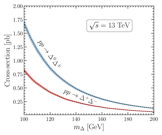
Fig. 1 shows the dominant Feynman diagrams for the production of the triplet-like Higgs states.999We obtain the leading-order Drell-Yan production cross-sections by using the UFO modules generated from SARAH Staub:2013tta ; Staub:2015kfa and Feynrules Degrande:2011ua ; Alloul:2013bka ; Degrande:2014vpa in MadGraph5_aMC_v3.5.3 Alwall:2011uj ; Alwall:2014hca with the NNPDF23_nlo_as_0118_qed parton distribution function Ball:2013hta . The higher-order corrections can be included via a factor, which at the next-to-leading order (NLO) in QCD matched with next-to-next-to-leading-logarithmic (NNLL) threshold resummation is 1.15 for the mass range of our interest Ruiz:2015zca ; Ajjath:2023ugn . Further, Refs. Ruiz:2015zca ; Ajjath:2023ugn showed that the NLO+NNLL differential -factors for heavy lepton kinematics are substantially flat, suggesting that naive scaling by an overall -factor is a very good approximation. Fig. 2 shows the Drell-Yan production cross-sections for the triplet-like Higgs states at the 13 TeV LHC, including the higher-order corrections via factor, as a function of their common mass. The SM-like Higgs is also DY-produced in the SM. However, the corresponding cross-sections are suppressed by the square of the small mixing angles and .
3.2 Decays of the SM-like Higgs
The properties of the SM-like Higgs boson have been studied in detail at the LHC Chatrchyan:2012jja ; Aad:2013xqa ; ATLAS:2016neq ; Langford:2021osp ; ATLAS:2021vrm ; ATLAS:2022vkf ; CMS:2022dwd . These data, particularly on and , provide nontrivial constraints on New Physics (NP) impacting the SM Higgs. It is customary to define the corresponding signal strengths for a decay mode , normalised to the SM value
| (48) |
where is the production cross-section of normalised to its SM value and MeV is the total decay width in the SM. For and , the partial widths are given by Chen:2013vi
| (49) | |||
| (50) |
where the fine-structure constant should be taken at the scale (since the photons are on-shell), and
Here and are the electric charge and the third component of the electroweak isospin of the SM fermion 101010In our notation, for the left(right)-handed fermions in weak isodoublets (isosinglets). running in the loop, respectively, is the number of colours (3 for quarks and 1 for leptons). We also defined
| (51) |
the functions are collected in Appendix B, and the Higgs coupling to fermions normalised to its SM value is
| (52) |
The other SM Higgs signal strengths (, , , , and ) are given by , and the one for is given by .
These expressions must be compared to the measurements of CMS and ATLAS for the , and signal strengths using the full run 2 data at the 13 TeV LHC. Combining their most recent measurements: CMS:2021kom and ATLAS:2022tnm , we get the weighted average
| (53) |
On the other hand, the collaborations themselves performed a combined analysis of their measurements ATLAS:2020qcv ; CMS:2022ahq in Ref. ATLAS:2023yqk and reported
| (54) |
Note that this measured value is in mild tension () with the SM expectation. The PDG average ParticleDataGroup:2022pth of the signal strength based on the LHC measurements ATLAS:2016neq ; CMS:2022dwd ; ATLAS:2020rej gives
| (55) |
While the signal strength puts a constraint on the mixing angle
| (56) |
the and signal strengths impose non-trivial constraints on , and . Note that their dependence on stems from the coupling, see Eq. (51). Figs. 3 and 4 show their dependence on and plane for GeV and GeV (left) and GeV (right).111111Understandably, the chosen values for and might seem arbitrary at this point. However, as we see later in Section 4.1, these values for are preferred by the -mass world average, including/excluding the CDF-II measurement. Further, we find later in Section. 4.3 that ATLAS di-photon data strongly prefer a Higgs triplet with GeV. As we see, is favored by the measurements for GeV. The same follows for . The reverse that is favoured by the measurements is largely true for (corresponding plot not shown for brevity). As expected, a positive correlation between and in the vs plane can be seen. That is the parameter space predicting a larger-than-expected predicts a larger-than-expected , and vice-versa. However, since the latter is beset with quite a large error, it is not difficult to simultaneously accommodate both measurements.

3.3 Decays of the triplet-like Higgses and
The triplet-like Higgs states and have two dominant classes of decays:
-
decays into two SM particles (on-shell or off-shell), either at tree-level to , , , , or at the loop level to , , . Likewise decays to , , . The asterisk signals a possible off-shellness.
-
Even though kinematically suppressed due to the small mass splitting, and could decay into one another and an off-shell -boson, often referred to as cascade decays.
The tree-level decay rates for the triplet-like Higgs are given by
where
and the loop-induced decays, with at least one massless gauge boson in the final state, are given by
where is the strong coupling constant,
with
and all the loop functions or form factors used in the Higgs decays are collected in Section B.
Finally, for masses slightly below the threshold, can decay into one on–shell and one off-shell top quarks, . As in the MSSM or 2HDM, the below-threshold branching ratios can be significant only very close to the threshold. Therefore, this decay is negligible in the mass region of our interest and thus not considered further for brevity.
While we provide the leading order decay rates here, QCD corrections can be sizable. To estimate them, we use the higher-order corrections reported in the CERN Yellow Report 3 LHCHiggsCrossSectionWorkingGroup:2013rie for and appropriately apply them to decays for our numerical estimation.
The dominant decay rates for the triplet-like charged Higgs are given by Rizzo:1980gz ; Keung:1984hn ; Djouadi:1997rp ; Djouadi:2005gi ; Djouadi:2005gj
where
Having provided all the decay rate expressions, a brief discussion on their dependence on the free model parameters is in order. Note that, for the mass range of our interest, any of the heavy SM particles can be off-shell. However, for brevity, we omit the asterisk sign signaling this hereinafter. The tree-level decays of depend on three parameters, namely , and , while those of depend on and only, except for which also depends on . The cascade and loop-induced decays depend additionally on the mass-splitting . As discussed in Sec. 2.2, the requirement of vacuum stability and perturbative unitarity, together with the EW precision data, restricts the mass-splitting to a few GeV. Therefore, on account of this small mass-splitting, the cascade decays are generally suppressed. Further, the dependence of the tree-level decays on drops out as long as GeV. Consequently, for the -range favoured by -mass measurements (see Sec. 4.1), the tree-level decays are reasonably independent of . However, the loop-induced decays crucially depend on .
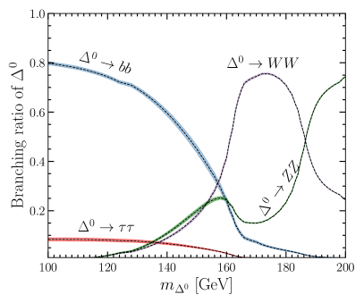
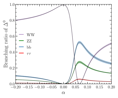
In Fig. 5, we show the variation of the dominant branching ratios of the triplet-like Higgs , including the corresponding uncertainties, as a function of its mass (left) and the mixing angle (right). The uncertainties are estimated by propagating the errors on the , , and decays of a hypothetical SM-like Higgs with mass reported in the CERN Yellow Report LHCHiggsCrossSectionWorkingGroup:2013rie . For definiteness, we take GeV. Further, we take for the left plot and GeV for the right one. While exclusively decays into for , the other modes become relevant for . In particular, for , the mode dominates over the rest for up to close to the kinematic threshold, beyond which the gauge-boson modes and become the primary ones. While for (corresponding plot not shown for brevity), the and modes are relevant, with the latter dominating over the former much before the threshold. However, the mode vanishes for ; see the right plot. Before moving further, a brief comment on the decay is in order. Though this mode is not suppressed by , it is suppressed by the kinematic phase space for , thus not relevant for the mass range of our interest.
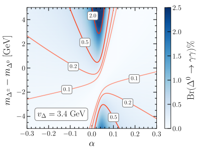
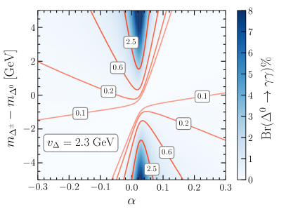
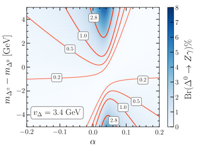
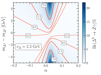
Figs. 6 and 7 show Br and Br in the vs plane for GeV and GeV (left) and GeV (right). As we see, in the vicinity of degenerate mass-spectrum for the triple-like Higgs states, both the and branching ratios are %–%.
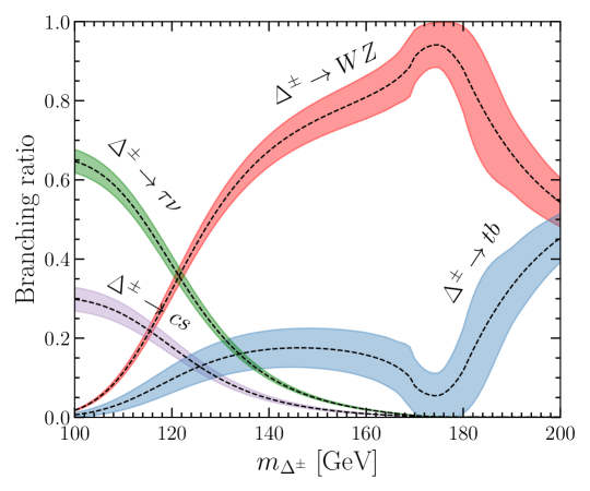
In Fig. 8, the dominant branching ratios of the charged Higgs , including the corresponding uncertainties, are shown as a function of its mass . Once again, the uncertainties are estimated by propagating the errors on the , , and decays of a hypothetical SM-like Higgs with mass reported in the CERN Yellow Report LHCHiggsCrossSectionWorkingGroup:2013rie . For definiteness, we take GeV and . For low , the most dominant decay mode is . While for intermediate , which is also the mass range of our interest, the mode dominates over the rest, with the mode dominating for high .
Finally, a brief comment on the decay is in order. As mentioned earlier, among all decays of , only the mode depends on . This decay is suppressed by as well as the kinematic phase space through the coupling , and thus not shown in the plot. In fact, it vanishes for . That said, this can be relevant for sizable and .
4 Phenomenology
4.1 mass
The mass GeV as measured by the CDF II collaboration CDF:2022hxs is significantly larger than the ATLAS measurement ATLAS:2023fsi as well as the LHCb measurement LHCb:2021bjt . Combining these measurements with those from the D0 experiment Abazov:2009cp ; D0:2013jba ; LHCb:2021bjt ; Aaboud:2017svj at the Tevatron, and the ALEPH, DELPHI, L3 and OPAL experiments at the LEP ALEPH:2013dgf , the LHC-TeV MW Working Group LHC-TeVMWWorkingGroup:2023zkn has obtained a world average
| (57) |
Comparing this with the SM prediction of GeV deBlas:2022hdk , the discrepancy of MeV amounts to . Since there is a tension between the most precise CDF-II measurement and the rest, removing the former increases the compatibility within the fit and leads to a lower average of
| (58) |
is obtained. Therefore, the world average, including the CDF-II measurement, requires GeV, while excluding CDF-II, one finds GeV.121212There is a recent update on the measurement of by ATLAS which finds a slightly heavier GeV ATLAS:2024erm compared to their previous analysis ATLAS:2023fsi based on the same dataset. However, the said combination did not consider the updated ATLAS measurement. Furthermore, after this combination was performed, CMS published a new measurement GeV CMS:2024nau , which agrees well with the world average excluding the CDF-II measurement. Including these updates might significantly reduce the world average and thus would imply a slightly lower value for . However, the specific value for is immaterial for our analysis as long as GeV. In the rest of this work, we fix GeV or GeV.
4.2 Multi-lepton signature from DY production
Drell-Yan production of the triplet-like Higgs bosons, and , with their decays and lead to final states with multiple charged leptons. Two representative Feynman diagrams for these processes are shown in Fig. 9.
As discussed in Sec. 3.3, low-mass triplet-like charged Higgs dominantly decays to ; see Fig. 8. Consequently, their pair production and subsequent decays, as shown in Fig. 10, leads to a final state with a pair of -leptons and missing transverse momentum, which is the identical collider signature as supersymmetric partners of -leptons () promptly decaying into a and a (massless) neutralino. This has been searched for by CMS and ATLAS collaborations ATLAS:2019gti ; CMS:2019eln ; CMS:2022rqk ; ATLAS:2024fub .
Using the full run 2 dataset at the 13 TeV LHC, CMS CMS:2022rqk has obtained 95% confidence level (CL) upper limits on the cross-section as a function of the mass. On the contrary, ATLAS ATLAS:2024fub observed a stronger limit than expected; however, they do not provide upper limits on the cross-section. We thus use the CMS result in Ref. CMS:2022rqk to constrain the triplet-like charged Higgs .
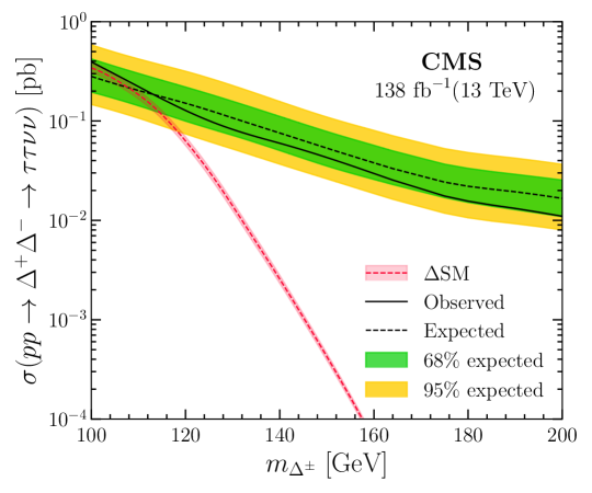
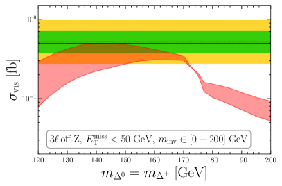
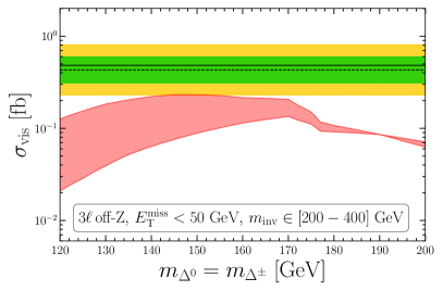
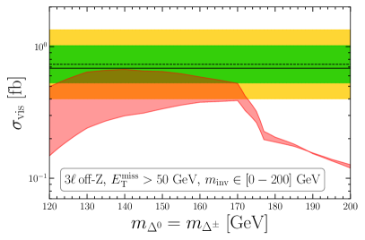
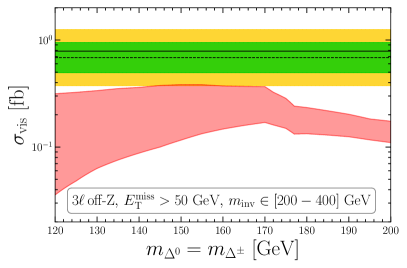
The CMS expected and observed 95% CL upper limits on the signal cross-section , taken from Ref. CMS:2022rqk , are shown in Fig. 11. The inner green and outer yellow bands around the dotted line indicate the 68% and 95% CL regions. The red line and the thin-shaded band indicate the model prediction for the signal cross-section, including the NLO+NNLL QCD corrections and uncertainties. The QCD corrections are taken from Refs. Ruiz:2015zca ; Ajjath:2023ugn , and the uncertainties are estimated by propagating the ones on the cross-section and branching ratios reported in Refs. Ruiz:2015zca ; Ajjath:2023ugn and Ref. LHCHiggsCrossSectionWorkingGroup:2013rie , respectively. This excludes with masses below 110 GeV at 95% CL.
For higher masses of the triplet-like Higgses, i.e. GeV, the decays to and become relevant. The most relevant signatures stem from the subsequent decays to leptons, which, compared to hadronic final states, have a considerably smaller SM background and, thus, superior constraining power. Since there is no dedicated search for this signature of our model,131313Several multi-lepton searches have been performed using the full run 2 data by CMS and ATLAS, see e.g. Refs. CMS:2019lwf ; CMS:2021zkl ; ATLAS:2021yyr ; ATLAS:2021wob ; ATLAS:2022nmi ; ATLAS:2022yhd ; ATLAS:2022pbd . However, most of these searches probe specific models and, like for instance Ref. ATLAS:2022yhd and Ref. ATLAS:2021yyr consider events with high lepton invariant masses and/or high missing transverse momenta. Being tuned for specific models, these searches exploit very distinctive event features, such as resonances in invariant-mass distributions and high missing transverse momenta, and are thus not expected to be sensitive in probing the SM. Ref. Butterworth:2023rnw used several SM measurements implemented in the Contur toolkit, and find that the four-lepton search by ATLAS ATLAS:2021kog is the most constraining one. They excluded with mass in the 180–200 GeV range for small ; while for sizeable , the constraints are easily avoided. Here, we will make use of the model-independent multi-lepton search by ATLAS ATLAS:2021wob , which entails inclusive event selection and thus covers a large phase space of signatures. This search considers 22 signal regions (SRs) and analyses them model-independently by putting limits on the visible cross-sections.
The three and four charged-lepton events are categorised into several orthogonal SRs based on the number of leptons, the presence/absence of a lepton pair presumably originating from a -boson decay (on-/off- lepton pair141414A pair of same-flavour and oppositely charged leptons with di-lepton invariant mass within the 10 GeV window of the -boson mass is referred to as on- lepton pair. A lepton that does not form an on- lepton pair with any other lepton in the event is called off-.) and the missing transverse momentum:
-
on- GeV,
-
on- GeV,
-
off- GeV,
-
off- GeV,
-
on- GeV,
-
on- GeV,
-
off-,
with each () SRs further divided into four(two) bins of the invariant mass of the leptons: 0 GeV–200 GeV, 200 GeV–400 GeV, 400 GeV–600 GeV and GeV (0 GeV–400 GeV and GeV), thereby resulting in 22 SRs in total.
We recast this search to constrain the SM by simulating the processes and with and for between 120 GeV and 200 GeV using the UFO modules generated from SARAH Staub:2013tta ; Staub:2015kfa 151515We also build the UFO model files at NLO using FeynRules Degrande:2011ua ; Alloul:2013bka ; Degrande:2014vpa . While it is desirable to perform the simulations at NLO, in order to reduce the computational resources needed for our analysis, we perform them at LO and then naively scale the production cross-section to account for the NLO+NNLL QCD corrections as discussed in Sec. 3. in MadGraph5_aMC_v3.5.3 Alwall:2014hca ; Frederix:2018nkq with the NNPDF23_nlo_as_0118_qed parton distribution function Ball:2013hta . The simulated parton-level events are then passed through the regular chain of tools, namely Pythia 8.3 Sjostrand:2014zea and Delphes 3.5.0 deFavereau:2013fsa , to simulate the effect of subsequent decays of the unstable particles, radiations, showering, fragmentation and hadronisation, various detector effects, and particle-level object reconstruction.
For the selection of various objects, viz. photons, leptons (electrons and muons) and jets (including -tagged and -tagged jets), we meticulously follow the said ATLAS search ATLAS:2021wob . In particular, we appropriately tune the Delphes card for the ATLAS detector to take into account various object reconstruction, isolation and selection requirements and jet tagging efficiencies. We use the anti- algorithm Cacciari:2008gp implemented in FastJet 3.3.4 Cacciari:2011ma to reconstruct jets. The missing transverse momentum (with magnitude ) is estimated from the momentum imbalance in the transverse direction associated with all reconstructed objects in an event. Finally, we apply the event selections and categorise the selected events according to the signal regions in Refs. ATLAS:2021wob .
While the branching ratio of the dominant modes depends only on its mass, the partial widths of depend on in addition (see Sec. 3.3). While exclusively decays to for , the and modes become relevant for non-zero . In fact, for , the rate to can even be zero, as can be seen in Fig. 5. However, in this case, the decay to , which also leads to a sizable number of leptons, can be sizable. We will therefore consider the two limiting cases of Br and Br, where in the latter case non-zero Br is considered. We then interpolate the two limiting cases as a function of the triplet mass.
Results
In Fig. 12, we show the upper limits on the visible signal cross-section observed by ATLAS ATLAS:2021wob and the SM model predictions for the SRs which give the most relevant constraints. The dashed and solid lines, respectively, indicate the expected and observed limits. The inner green and outer yellow bands around the dashed lines indicate the regions containing 68% and 95% of the distribution of limits expected under the background-only hypothesis. The red-shaded bands indicate the SM model predictions for the corresponding signal cross-section, with the upper (lower) line of each band corresponding to a 100%(0%) branching ratio for . One can see that while the predicted effect is, in many cases, close to the observed limits, the SM cannot be excluded with this model-independent multi-lepton search by ATLAS. However, run 3 and high-luminosity data Cepeda:2019klc will be able to test the SM in the mass region below 200 GeV.
4.3 Associated production of the triplet-like Higgs and resonant di-photon signatures:
Drell-Yan production of the triplet-like Higgs states via an off-shell -boson, i.e. with leads to final states with a photon pair (di-photon) and additional particles and/or missing transverse momentum from the decay of . This signature is shown in Fig. 13. The mass of can be reconstructed from the di-photon invariant mass () distribution.
In the SM model, has a branching ratio of %–% (see Fig. 6 and the relevant discussion in Sec. 3.3). Though this decay rate is much lower than the ones for several other channels such as (see Fig. 5), the sensitivity of the di-photon final state is enhanced by the clearness of the corresponding detector signal as well as the smaller SM background.
An analysis of has been performed by ATLAS, targeting the SM Higgs ATLAS:2023omk . This search considers 22 SRs categorized by , the objects produced in association with the di-photon; see Table 3 of Ref. ATLAS:2023omk for the definitions of the SR. In addition, ATLAS has released a search for non-resonant di-Higgs production, which includes ATLAS:2024lhu not covered in the previous analysis. Both these searches provide distributions in the 105 GeV–160 GeV range, thereby covering part of the mass range of our interest for the SM.
Because the ATLAS analyses performed a model-independent analysis of the associated production of the SM Higgs, no channels were combined, and the hypothesis of a BSM Higgs was not considered. However, the sidebands can be used to perform a search for BSM Higgses; within the SM, all signal regions are correlated so that they can be combined.
For this, we simulate the process for 50 values of in the 105 GeV–157 GeV range. As we did for the multi-lepton search in Sec. 4.2, we use the same set of tools to recast this search. Once again, we appropriately tune the delphes card for the ATLAS detector to take into account various object reconstruction, isolation and selection requirements. Following that, we apply the event selections and categorise the selected events into several SRs as in Ref. ATLAS:2023omk ; ATLAS:2024lhu .
Effects in the relevant SRs
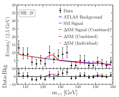
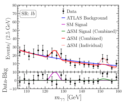
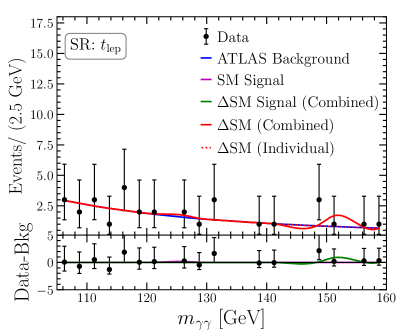
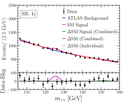
Given the dominant decay modes of ( and ) and their subsequent decays to leptons, quarks and neutrinos, we expect that the SRs targeting leptons (), taus (), multiple jets () and are the most sensitives ones. Those targeting top quarks are expected to become relevant for larger . Among the three SRs related to top quarks, the one targeting hadronically decaying top quarks is not sensitive to the signal of our model for the mass range of our interest because it is targeting hadronically decaying top quarks from production.161616ATLAS uses a boosted decision tree (BDT) for top-quark reconstruction and requires a tight cut of 0.9 on the BDT score. The corresponding signal in the SM model consisting of a bottom quark and an (off-shell) top quark being quite different, the resulting efficiency is expected to be very small, thus rendering this SR irrelevant for the mass range of our interest.
Before proceeding, a few comments on SRs are in order. The SR has been considered by both the Ref. ATLAS:2023omk and Ref. ATLAS:2024lhu . Since the latter applies a -jet veto, this SR is nearly uncorrelated with the SR considered in Ref. ATLAS:2023omk . This leads us to use the SR of Ref. ATLAS:2024lhu . Furthermore, for both the and SRs of Ref. ATLAS:2024lhu , they use a BDT to further categorise the events into three categories based on the BDT score. Since the corresponding weight files are not available yet, it would be a highly non-trivial task to appropriately implement the same BDTs for a little too gain in sensitivity. Therefore, instead of implementing the BDTs, we take a conservative approach to adding the event yields of all three BDT categories to recover the yields that would have resulted after the event selections (and before the BDTs). Concerning the SR, since ATLAS has observed no event, we treat the entire range as a single bin. Similarly, we do not show the GeV SR since very few events have been observed and it is correlated to the other MET categories.171717We checked that for our best-fit point for 152 GeV, events are predicted while 1 NP event is observed, showing the consistency. Finally, while scaling by an overall -factor of 1.15 at the cross-section level accounts for the NLO+NNLL QCD correction in the production of the triplet Higgs states, additional correction accrues from enhanced selection efficiencies. This is particularly important for the SRs targeting high jet activity because of gluon radiation. To estimate this, we simulate the corresponding signal at NLO and find an additional correction factor 1.2 for the SR.
After simulating the effect in all signal regions given by ATLAS, taking into account the consideration above, it turns out that the 10 SRs listed in Table 1 are relevant in the SM model for the mass range of our interest. This means that the other SRs lead to such weak constraints on Br that disregarding them in a combined analysis has virtually no impact on the result.
| Target | Signal region | Detector level selections | Correlation |
| High jet activity ATLAS:2023omk | , | – | |
| Top ATLAS:2023omk | , | – | |
| , | – | ||
| Lepton ATLAS:2023omk ; ATLAS:2024lhu | or | () | |
| , , , GeV (only for -channel) | () | ||
| Tau ATLAS:2024lhu | 1 | , , , GeV | |
| ATLAS:2023omk | GeV | GeV | ( GeV) |
| GeV | GeV | ( GeV) | |
| GeV | GeV | – |
Background (re)fitting
To signals arising from BSM production, as in our case, the background consists of two components: resonant and continuum. The resonant component arises from the SM Higgs boson production and thus manifests itself as a narrow peak in the spectrum. The continuum component, depending on the SRs, arises from the production of two initial/final-state photons, the misidentification of jets and the production of EW bosons and top quarks. The continuum backgrounds are estimated from data by fitting the spectrum in the mass range 105 GeV–160 GeV with an analytic function with free parameters. Note that those estimated by ATLAS in Refs. ATLAS:2023omk ; ATLAS:2024lhu are obtained assuming there is only a single resonance at 125 GeV, i.e. the SM Higgs. On the contrary, in the SM model, there is another resonance at , i.e. the triplet-like Higgs, albeit with different signal strength. This resonance manifests itself as a narrow peak in the spectrum, much like the one at 125 GeV. Consequently, we need to (re)estimate the continuum background from a (re)fit to the data. ATLAS follows the procedure spurious-signal test ATLAS:2018hxb to select a background function for a given SR from a number of candidate functions such as power-law functions, Bernstein polynomials, and exponential functions (of a polynomial), to ensure small potential bias in the extracted signal yield compared to the experimental precision. However, for the sake of simplicity, we use the following common function for all SRs (except the SR, for which the yields are too small to fit a distribution):
| (59) |
where and are the free parameters which are independent across SRs, TeV is the LHC run 2 centre-of-mass energy. This function is fitted with the data subtracted by the resonances—SM Higgs at 125 GeV and triplet-like Higgs at —to estimate the (re)fitted continuum background.
Statistical model
The data are interpreted as briefly described below. A likelihood function is built from the number of observed and (re)fitted SM signal-plus-background events. Assuming the bins in the spectrum for a given SR as independent number-counting experiments, the likelihood is modelled as
| (60) |
where runs over the 22 bins in the spectrum in the 105 GeV–160 GeV range and represents the parameter of interest or signal strength: branching ratio, Br in our case (this choice to be justified shortly). Here, as is typically done for number-counting experiments, the Poisson distribution is used to compare the measured data with the modelled expectation comprising of a signal yield and a background yield . Then, the global likelihood for the measurements is obtained as the product of the likelihood functions for the relevant SRs. Finally, the profile likelihood ratio test statistics Cowan:2010js is given by
where refers to the value of that maximises the likelihood. This test statistics asymptotically follows a distribution such that approximate 68% and 95% CL ( and ) intervals can be easily constructed by requiring and , respectively. Note that we allow for an unphysical negative to take into account the effect of downward fluctuations of the background.
Results
In Figs. 14 and 15, we show the fit to the di-photon invariant mass distributions for the relevant signal regions listed in Table 1. The data and continuum backgrounds taken from the ATLAS analyses are shown in black (points with error bars) and blue, respectively. Also shown are the 125 GeV SM Higgs signals (magenta) and 152 GeV SM triplet Higgs signals with Br (green). For brevity, we do not show the (re)fitted continuum backgrounds; the (re)fitted SM signal-plus-backgrounds are shown in red. Note that the SM benchmark chosen here is occasioned by our findings later in this section that there is a strong preference for Br at 152 GeV when all relevant SRs are statistically combined.
Now, we put upper limits on the parameter of interest, Br. While this is trivially calculable, as discussed in Sec. 3.3, it crucially depends on the triplet mass , the mixing angle , the mass-splitting (through the coupling) and the triplet VEV . Hence, rather than varying these parameters, we subsume them within a single observable Br, which is of great interest as far as the LHC search program for additional Higgs is concerned. 95% CL upper limits on Br as a function of the triplet Higgs mass for various SRs are shown in Fig. 16. For brevity, we only show the SRs that are most constraining, i.e. provide relevant bounds on Br.
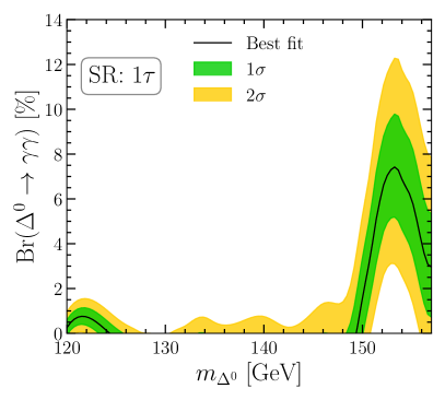
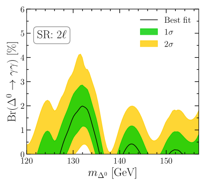
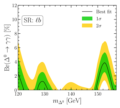
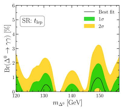
We then proceed to find the preferred ranges for Br as a function of for the relevant SRs. The obtained best-fit values, along with the and ranges, are shown in Figs. 17 and 18. For reasons mentioned earlier, here, we do not show the corresponding plots for and GeV SRs. Interestingly, all relevant SRs display a preference for a non-zero decay rate around 152 GeV.
Finally, we combine the 10 relevant SRs, including their correlations, to obtain the combined preferred ranges for Br as a function of , as shown in Fig. 19.181818Note that there are moderate correlations among some SRs, in particular, among the ones. However, we checked that removing the GeV SR from the fit has a very small impact on the final result. We see a strong preference for a non-zero Br in the 150 GeV–155 GeV range. This is most pronounced at 152 GeV with Br, and the corresponding significance amounts to .
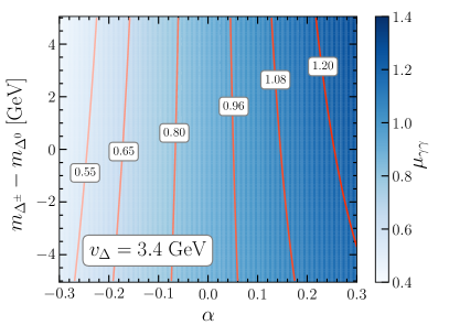
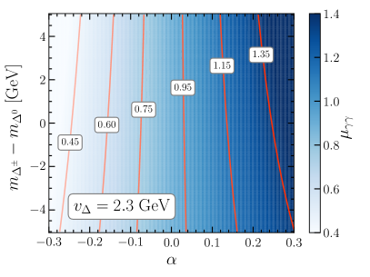
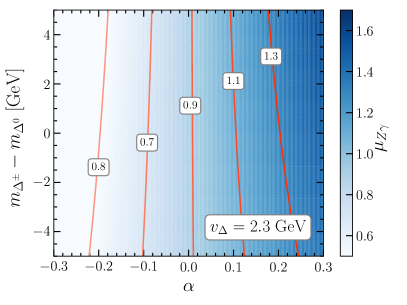
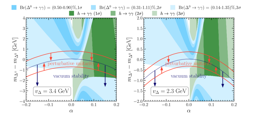
For the sake of phenomenological interest, we have subsumed the free parameters of the SM model—the triplet mass , the mixing angle , the mass-splitting and the triplet VEV —into a single observable Br. Before closing this section, we closely look at how the preferred di-photon decay rate can be obtained. For a given and , Br depends on and . In Fig. 20, we show the preferred regions in the vs plane for GeV and two values of : 4.1 GeV (left) and 2.7 GeV (right), corresponding to the best-fit values obtained from the world -mass fit with and without including the CDF-II measurement. The band between the two orange lines satisfies perturbative unitarity, and the region below the blue line leads to a stable vacuum at the EW scale. The green regions are allowed by the SM Higgs to di-photon signal strength CMS:2021kom ; ATLAS:2022tnm at (1.02-1.15), (0.96-1.22) and (0.90-1.29) levels. The (0.50–0.90%), (0.31–1.11%) and (0.14–1.35%) regions for Br are shown in violet. We see that the region (and also part of the region) preferred by the ATLAS searches are not in accordance with the vacuum stability and perturbative unitarity constraints. This demonstrates that while we have growing evidence for a 152 GeV triplet-like Higgs produced in association with leptons (including -leptons), quarks (including -quarks) and neutrinos, the SM should be superseded by BSM models with additional fields at or above the EW scale so as to restore the stability of the vacuum and perturbativity of the theory.
4.4 Higgs to search in the final state
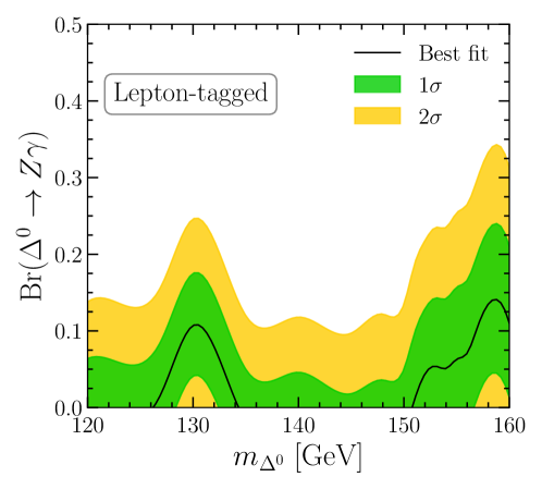
Similar to the di-photon mode, can have a branching ratio of about %–% (see Fig. 7 and the relevant discussion in Sec. 3.3). Experimentally, the final state resulting from the leptonic decay of ( with ) is the most accessible since the leptons are highly distinctive. CMS has recently performed such a pertinent search with the full run 2 data in Ref. CMS:2022ahq . This search categorises the events into three broad mutually exclusive SRs: Lepton-tagged, Dijet, and Untagged, further categorising the latter two into 3 and 4 SRs. We meticulously recast this search in the context of the SM and find that only the Lepton-tagged SR is relevant. In Fig. 21, we show the preferred ranges for Br as a function of . Though the current bounds are not competitive with di-photon searches, they are expected to become relevant with high-luminosity LHC data Cepeda:2019klc .
5 Summary and Outlook
Though the ongoing LHC search program for new particles has not led to any discovery yet, it has, nonetheless, unveiled several hints for new particles in the form of “anomalies” Crivellin:2023zui . This includes the multi-lepton anomalies vonBuddenbrock:2019ajh ; Fischer:2021sqw which points towards the existence of a new Higgs with a mass of GeV which dominantly decays to vonBuddenbrock:2017gvy . Furthermore, the re-analyses of the sidebands of the ATLAS and CMS Higgs boson searches indicate the presence of a new narrow resonance with a mass around 152 GeV produced in association with leptons, quarks, and neutrinos Crivellin:2021ubm ; Bhattacharya:2023lmu .
In this context, it has been shown that the excesses are consistent with the Drell-Yan production of a GeV Higgs from a scalar triplet with , with a significance of Ashanujjaman:2023etj ; Crivellin:2024uhc , which predicts a positive-definite shift in the mass, in agreement with the global fit. Furthermore, its neutral component decays dominantly to , as suggested by the multi-lepton anomalies.
Motivated by this, we have detailed the Higgs triplet model and its phenomenology in this work. In particular, we have studied the tree-level perturbative unitarity and bounded-from-below constraints on the scalar potential. Further, we have discussed various possible vacua configurations and the stability of the neutral ones against the charge-breaking ones, which is discussed in Appendix C. We showed that the absence of tachyonic modes in the Higgs sector suffices to ensure that the desired EW vacuum corresponds to the global minimum of the potential. Combined, these constraints delineate the theoretically allowed parameter space within the perturbative regime and, together with the constraints from the parameter, drive the triplet-like neutral and charged Higgs states to be quasi-mass-degenerate.
We have discussed the production and decays of the Higgs states, including the , and decays, which put non-trivial constraints on the model parameter space. Furthermore, we have detailed their phenomenology at the LHC based on three types of final states: stau-like signature, multi-lepton and final states. The findings are summarised below.
-
Low-mass ( GeV) triplet-like charged Higgs dominantly decays to . Therefore, the process leads to final states involving a pair of -leptons and missing transverse momentum, which is akin to the collider signature of stau. Our reinterpretation of the corresponding CMS search CMS:2022rqk excludes triplet-like charged Higgs with a mass below 110 GeV at 95% CL.
-
For triplet-like Higgs bosons with higher masses ( GeV) the dominant decays modes are and . Therefore, their Drell-Yan production can lead to final states with multiple charged leptons from the leptonic decays of and . To probe the SM, we recast a recent model-independent analysis of ATLAS ATLAS:2021wob involving three and four leptons in the final state. Our analysis shows that for some SRs, the predicted effect is close to the observed limit of ATLAS, but SM cannot be excluded from this search. However, run 3 and high-luminosity LHC data will be able to test the signatures of the SM in multi-lepton final states.
-
The associated production of the triplet-like Higgses and their prompt decays to di-photon lead to final states. We have performed two such pertinent searches by ATLAS. We have performed a (re)fit to the data to determine the continuum background and a likelihood-based statistical interpretation to find that, out of the 25 signal regions considered, 10 of them put stringent limits on the triplet-like Higgs, particularly on its di-photon branching ratio Br. Interestingly, all relevant signal regions show a weakening of the limits around 125 GeV–130 GeV and 152 GeV. More importantly, there is a strong preference for a non-zero di-photon decay rate in the 150 GeV–155 GeV range. When all relevant SRs are statistically combined, this is most pronounced at 152 GeV with the corresponding branching ratio of about 0.7% and the corresponding significance of about . While such a sizable branching ratio to di-photons is easily achievable in the SM, part of this model parameter space consistent with the di-photon signal strength of the SM Higgs is in tension with the vacuum stability and perturbative unitarity.
The last point, i.e. the preferred range for the di-photon decay rate is in tension with the vacuum stability and perturbative unitarity, demonstrates that while we have growing evidence for a 152 GeV Higgs produced in association with leptons, quarks and neutrinos, the SM is not expected to be the final theory superseding the SM. In fact, with additional fields at or above the EW scale, the problem of the large di-photon rate in unstable field configurations can be solved in (at least) three non-exclusive ways. Additional field(s) can
-
modify the (effective) scalar potential such that the vacuum stability is restored at larger field values,
-
lead to loop contributions to ,
-
allow for a larger VEV of the triplet by cancelling its effect in the parameter as in the Georgi-Machacek model Georgi:1985nv , thereby enlarging the region with the stable EW vacuum.
and are possible, e.g. by introducing additional charged Higgs bosons; an interesting UV-realisation of this is the 2HDMS: the SM extended with a second Higgs doublet and a singlet Coloretti:2023yyq . In addition to explaining the di-photon excess in associated production Banik:2024ftv this model can address the significant tensions in differential top quark distributions ATLAS:2023gsl as shown in Ref. Banik:2023vxa and lead to baryogenesis via a two-step phase transition Inoue:2015pza .
In summary, the SM, analysed in detail in this article, represents a step towards the establishment of a model that can simultaneously explain the multi-lepton anomalies and the narrow resonance in associated production with a mass of 152 GeV. However, more data and improved SM predictions are necessary to arrive at the conclusive model superseding the SM.
Appendix A Feynman rules for the SM
Here, we provide the Feynman rules for vertices involving the triplet fields. All momenta are considered to be incoming. We take the positively charged components of the triplets as particles and the negatively charged ones as antiparticles. Consequently, particle flow arrows point in the direction of particle momentum, while they point opposite to the momentum direction for antiparticles. We use the shorthand notations and .
Appendix B Loop functions
Appendix C Stability and charge-breaking minima
The scalar potential in Eq. (2.1), in principle, can have several stationary points—both electric charge-conserving and charge-breaking. In this section, we discuss all possible stationary points and obtain the necessary conditions for the desired EW vacuum to be the global minimum of the model by calculating the differences in the potential depths between the desired EW vacuum and others, some of which might not be phenomenologically viable. It might be argued that absolute stability of the vacuum is not a necessary requirement since the vacuum could be meta-stable, i.e. have, a lifetime longer than the age of the Universe. While the latter is certainly an interesting possibility, it would require a detailed calculation of the tunnelling time of the vacuum into the global minimum, which is beyond the scope of this work. Therefore, we restrict to the stronger requirement that the vacuum is at the global minimum.
Concerning the gauge choice, note that we can always absorb three real scalar component fields via a suitable gauge choice (such as a rotation in field space). For definiteness, we choose the SM unitary gauge, wherein the doublet is reduced to a neutral, real component. As a consequence, the doublet VEV is, without loss of generality, always real and neutral. Further, the triplet being real (see Eq. (2) and the text thereafter), the corresponding VEVs are also real.
The SM can have several stationary points as listed in Table 2. Of these, three are charge-conserving minima: , and , referred to as normal minima, wherein the neutral components of the scalar fields get VEVs. On the contrary, there are two possible charge-breaking (CB) minima. Such a scenario exists when electric charge-carrying VEVs appear after spontaneous symmetry breaking. The occurrence of CB vacuum results in a non-zero photon mass, which is incompatible with electromagnetic observations.
| N1 | |||
|---|---|---|---|
| N2 | |||
| N3 | |||
| CB1 | |||
| CB2 |
N1 stationary point
The N1 stationary point corresponds to the vacuum structure where both and get VEVs:
| (61) |
This vacuum structure has been detailed in Section 2.
N2 stationary point
The N2 stationary point corresponds to the vacuum structure where only gets VEV:
| (62) |
The minimization condition for this vacuum configuration is
| (63) |
To get the correct electroweak symmetry breaking for this vacuum configuration, we need GeV. Also, to get N2 extremum, we require , thereby restoring the global symmetry of the potential in Eq. (2.1). The consequence is the degenerate mass spectrum for the triplet scalars: . The scalar masses are given by,
| (64) | |||
| (65) |
N3 stationary point
The N3 stationary point corresponds to the vacuum structure where only gets VEV:
| (66) |
As the absence of a doublet VEV would imply massless fermions, this extremum is in disagreement with observations. Therefore, we do not discuss this further.
CB1 stationary point
In the CB1 case, both the neutral and charged components of the triplet scalar, and get VEVs:
| (67) |
This configuration is the most generic CB vacuum. The minimization condition for this vacuum configuration is
| (68) | |||
| (69) | |||
| (70) |
CB2 stationary point
In the CB2 case, only the charged component of the triplet scalar, gets VEV:
| (71) |
The minimization condition for this vacuum configuration is
| (72) | |||
| (73) |
Condition for global minima
In this section, we will examine the stability of the normal minima, in particular, the N1 stationary point, which we assume to be the desired global minimum of the model. To this end, assuming that N1 or N2 coexists with the CB minima in some region of the model parameter space, we calculate the differences in potential depth between the co-existing minima. For N1 to be the global minimum, it is crucial that the potential depth at is lower than those of the co-existing minima.
To calculate the difference in potential depth between two co-existing minima, we follow the bilinear formalism detailed in Refs. Ferreira:2004yd ; Barroso:2005sm , see Refs. Ferreira:2019hfk ; Azevedo:2020mjg ; Hundi:2023tdq for recent works. Note that the potential in Eq. (2.1) is the sum of three homogeneous functions of order 2, 3 and 4 in the fields and :
| (74) |
Consequently, up to , can be expressed as a quadratic polynomial on the vector constructed from the bilinears , and . Therefore, we have
| (75) |
where
| (76) |
At any stationary point SP, the potential must follow the minimisation conditions, i.e. with denoting real scalar degree of freedoms of the model. Thus, we have
| (77) |
where the latter follows from Euler’s homogeneous function theorem. Therefore, the value of evaluated at SP is
| (78) |
Now, we define the gradient of along : and compute the product of evaluated at a stationary point with evaluated at a different stationary point:
| (79) | |||
| (80) |
Finally, subtracting these two equations, we get
| (81) |
In what follows, we present the bilinear vector for all possible stationary points and the differences in potential depth between the co-existing minima using Eq. (81).
| (82) |
| (83) | |||
| (84) | |||
| (85) | |||
| (86) | |||
| (87) |
where , and in Eq. (83), Eq. (84) and Eq. (85) are the physical masses evaluated at the stationary point, whereas those in Eq. (86) and (87) are evaluated at the stationary point. Therefore, as it turns out, the desired EW vacuum is indeed the global minimum of the model for as long as the scalars are not tachyonic, i.e. , and . While for , the normal minimum is the global minimum.
Acknowledgements.
S.A. acknowledges partial support from the National Natural Science Foundation of China under grant No. 11835013. The work of A.C. is supported by a professorship grant from the Swiss National Science Foundation (No. PP00P21_76884). S.P.M. acknowledges using the SAMKHYA: High-Performance Computing Facility provided by the Institute of Physics, Bhubaneswar.References
- (1) Particle Data Group Collaboration, R. L. Workman et al., “Review of Particle Physics,” PTEP 2022 (2022) 083C01.
- (2) HFLAV Collaboration, Y. S. Amhis et al., “Averages of -hadron, -hadron, and -lepton properties as of 2018,” Eur. Phys. J. C 81 no. 3, (2021) 226, arXiv:1909.12524 [hep-ex].
- (3) ALEPH, DELPHI, L3, OPAL, SLD, LEP Electroweak Working Group, SLD Electroweak Group, SLD Heavy Flavour Group Collaboration, S. Schael et al., “Precision electroweak measurements on the resonance,” Phys. Rept. 427 (2006) 257–454, arXiv:hep-ex/0509008.
- (4) P. W. Higgs, “Broken symmetries, massless particles and gauge fields,” Phys. Lett. 12 (1964) 132–133.
- (5) F. Englert and R. Brout, “Broken Symmetry and the Mass of Gauge Vector Mesons,” Phys. Rev. Lett. 13 (1964) 321–323.
- (6) P. W. Higgs, “Broken Symmetries and the Masses of Gauge Bosons,” Phys. Rev. Lett. 13 (1964) 508–509.
- (7) G. S. Guralnik, C. R. Hagen, and T. W. B. Kibble, “Global Conservation Laws and Massless Particles,” Phys. Rev. Lett. 13 (1964) 585–587.
- (8) ATLAS Collaboration, G. Aad et al., “Observation of a new particle in the search for the Standard Model Higgs boson with the ATLAS detector at the LHC,” Phys. Lett. B 716 (2012) 1–29, arXiv:1207.7214 [hep-ex].
- (9) CMS Collaboration, S. Chatrchyan et al., “Observation of a New Boson at a Mass of 125 GeV with the CMS Experiment at the LHC,” Phys. Lett. B 716 (2012) 30–61, arXiv:1207.7235 [hep-ex].
- (10) A. Crivellin and B. Mellado, “Anomalies in particle physics and their implications for physics beyond the standard model,” Nature Rev. Phys. 6 no. 5, (2024) 294–309, arXiv:2309.03870 [hep-ph].
- (11) CMS Collaboration, S. Chatrchyan et al., “Study of the Mass and Spin-Parity of the Higgs Boson Candidate Via Its Decays to Boson Pairs,” Phys. Rev. Lett. 110 no. 8, (2013) 081803, arXiv:1212.6639 [hep-ex].
- (12) ATLAS Collaboration, G. Aad et al., “Evidence for the spin-0 nature of the Higgs boson using ATLAS data,” Phys. Lett. B 726 (2013) 120–144, arXiv:1307.1432 [hep-ex].
- (13) ATLAS, CMS Collaboration, G. Aad et al., “Measurements of the Higgs boson production and decay rates and constraints on its couplings from a combined ATLAS and CMS analysis of the LHC collision data at and 8 TeV,” JHEP 08 (2016) 045, arXiv:1606.02266 [hep-ex].
- (14) ATLAS, CMS Collaboration, J. M. Langford, “Combination of Higgs measurements from ATLAS and CMS : couplings and -framework,” PoS LHCP2020 (2021) 136.
- (15) ATLAS Collaboration, “Combined measurements of Higgs boson production and decay using up to fb-1 of proton-proton collision data at TeV collected with the ATLAS experiment,”.
- (16) V. Silveira and A. Zee, “SCALAR PHANTOMS,” Phys. Lett. B 161 (1985) 136–140.
- (17) M. Pietroni, “The Electroweak phase transition in a nonminimal supersymmetric model,” Nucl. Phys. B 402 (1993) 27–45, arXiv:hep-ph/9207227.
- (18) J. McDonald, “Gauge singlet scalars as cold dark matter,” Phys. Rev. D 50 (1994) 3637–3649, arXiv:hep-ph/0702143.
- (19) T. D. Lee, “A Theory of Spontaneous Violation,” Phys. Rev. D 8 (1973) 1226–1239.
- (20) H. E. Haber and G. L. Kane, “The Search for Supersymmetry: Probing Physics Beyond the Standard Model,” Phys. Rept. 117 (1985) 75–263.
- (21) J. E. Kim, “Light Pseudoscalars, Particle Physics and Cosmology,” Phys. Rept. 150 (1987) 1–177.
- (22) R. D. Peccei and H. R. Quinn, “ Conservation in the Presence of Instantons,” Phys. Rev. Lett. 38 (1977) 1440–1443.
- (23) N. Turok and J. Zadrozny, “Electroweak baryogenesis in the two doublet model,” Nucl. Phys. B 358 (1991) 471–493.
- (24) W. Konetschny and W. Kummer, “Nonconservation of Total Lepton Number with Scalar Bosons,” Phys. Lett. B 70 (1977) 433–435.
- (25) T. P. Cheng and L.-F. Li, “Neutrino Masses, Mixings and Oscillations in Models of Electroweak Interactions,” Phys. Rev. D 22 (1980) 2860.
- (26) G. Lazarides, Q. Shafi, and C. Wetterich, “Proton Lifetime and Fermion Masses in an Model,” Nucl. Phys. B 181 (1981) 287–300.
- (27) J. Schechter and J. W. F. Valle, “Neutrino Masses in Theories,” Phys. Rev. D 22 (1980) 2227.
- (28) M. Magg and C. Wetterich, “Neutrino Mass Problem and Gauge Hierarchy,” Phys. Lett. B 94 (1980) 61–64.
- (29) R. N. Mohapatra and G. Senjanovic, “Neutrino Masses and Mixings in Gauge Models with Spontaneous Parity Violation,” Phys. Rev. D 23 (1981) 165.
- (30) CDF Collaboration, T. Aaltonen et al., “High-precision measurement of the boson mass with the CDF II detector,” Science 376 no. 6589, (2022) 170–176.
- (31) J. Butterworth, J. Heeck, S. H. Jeon, O. Mattelaer, and R. Ruiz, “Testing the scalar triplet solution to CDF’s heavy problem at the LHC,” Phys. Rev. D 107 no. 7, (2023) 075020, arXiv:2210.13496 [hep-ph].
- (32) J. Heeck, “-boson mass in the triplet seesaw model,” Phys. Rev. D 106 no. 1, (2022) 015004, arXiv:2204.10274 [hep-ph].
- (33) A. Strumia, “Interpreting electroweak precision data including the -mass CDF anomaly,” JHEP 08 (2022) 248, arXiv:2204.04191 [hep-ph].
- (34) I. Dorsner and I. Mocioiu, “Predictions from type II see-saw mechanism in ,” Nucl. Phys. B 796 (2008) 123–136, arXiv:0708.3332 [hep-ph].
- (35) P. Fileviez Perez, H. H. Patel, and A. D. Plascencia, “On the mass and new Higgs bosons,” Phys. Lett. B 833 (2022) 137371, arXiv:2204.07144 [hep-ph].
- (36) Y. Cheng, X.-G. He, F. Huang, J. Sun, and Z.-P. Xing, “Electroweak precision tests for triplet scalars,” Nucl. Phys. B 989 (2023) 116118, arXiv:2208.06760 [hep-ph].
- (37) T. G. Rizzo, “Kinetic mixing, dark Higgs triplets, and ,” Phys. Rev. D 106 no. 3, (2022) 035024, arXiv:2206.09814 [hep-ph].
- (38) J.-W. Wang, X.-J. Bi, P.-F. Yin, and Z.-H. Yu, “Electroweak dark matter model accounting for the CDF -mass anomaly,” Phys. Rev. D 106 no. 5, (2022) 055001, arXiv:2205.00783 [hep-ph].
- (39) M. Chabab, M. C. Peyranère, and L. Rahili, “Probing the Higgs sector of Higgs Triplet Model at LHC,” Eur. Phys. J. C 78 no. 10, (2018) 873, arXiv:1805.00286 [hep-ph].
- (40) Y. Shimizu and S. Takeshita, “ boson mass and grand unification via the type-II seesaw-like mechanism,” Nucl. Phys. B 994 (2023) 116290, arXiv:2303.11070 [hep-ph].
- (41) A. Crivellin, M. Kirk, and A. Thapa, “Minimal model for the -boson mass, , and quark-mixing-matrix unitarity,” Phys. Rev. D 108 no. 3, (2023) L031702, arXiv:2305.03081 [hep-ph].
- (42) T. A. Chowdhury, J. Heeck, A. Thapa, and S. Saad, “ boson mass shift and muon magnetic moment in the Zee model,” Phys. Rev. D 106 no. 3, (2022) 035004, arXiv:2204.08390 [hep-ph].
- (43) R. Dcruz and A. Thapa, “ boson mass shift, dark matter, and in a scotogenic-Zee model,” Phys. Rev. D 107 no. 1, (2023) 015002, arXiv:2205.02217 [hep-ph].
- (44) K. S. Babu, S. Jana, and V. P. K., “Correlating -Boson Mass Shift with Muon in the Two Higgs Doublet Model,” Phys. Rev. Lett. 129 no. 12, (2022) 121803, arXiv:2204.05303 [hep-ph].
- (45) G. Arcadi and A. Djouadi, “2HD+a light pseudoscalar model for a combined explanation of the possible excesses in the CDF measurement and with dark matter,” Phys. Rev. D 106 no. 9, (2022) 095008, arXiv:2204.08406 [hep-ph].
- (46) J. Kim, S. Lee, P. Sanyal, and J. Song, “CDF -boson mass and muon in a type-X two-Higgs-doublet model with a Higgs-phobic light pseudoscalar,” Phys. Rev. D 106 no. 3, (2022) 035002, arXiv:2205.01701 [hep-ph].
- (47) J. Kim, “Compatibility of muon , mass anomaly in type-X 2HDM,” Phys. Lett. B 832 (2022) 137220, arXiv:2205.01437 [hep-ph].
- (48) N. Chakrabarty, “Muon and -mass anomalies explained and the electroweak vacuum stabilized by extending the minimal type-II seesaw model,” Phys. Rev. D 108 no. 7, (2023) 075024, arXiv:2206.11771 [hep-ph].
- (49) T. A. Chowdhury, K. Ezzat, S. Khalil, E. Ma, and D. Nanda, “Higgs quadruplet impact on mass shift, dark matter, and LHC signatures,” Phys. Rev. D 109 no. 7, (2024) 075039, arXiv:2312.11833 [hep-ph].
- (50) T.-K. Chen, C.-W. Chiang, and K. Yagyu, “Explanation of the mass shift at CDF II in the extended Georgi-Machacek model,” Phys. Rev. D 106 no. 5, (2022) 055035, arXiv:2204.12898 [hep-ph].
- (51) S. Kanemura and K. Yagyu, “Implication of the boson mass anomaly at CDF II in the Higgs triplet model with a mass difference,” Phys. Lett. B 831 (2022) 137217, arXiv:2204.07511 [hep-ph].
- (52) S. Ashanujjaman, K. Ghosh, and R. Sahu, “Low-mass doubly charged Higgs bosons at the LHC,” Phys. Rev. D 107 no. 1, (2023) 015018, arXiv:2211.00632 [hep-ph].
- (53) D. A. Ross and M. J. G. Veltman, “Neutral Currents in Neutrino Experiments,” Nucl. Phys. B 95 (1975) 135–147.
- (54) J. F. Gunion, R. Vega, and J. Wudka, “Higgs triplets in the standard model,” Phys. Rev. D 42 (1990) 1673–1691.
- (55) T. Blank and W. Hollik, “Precision observables in models with an additional Higgs triplet,” Nucl. Phys. B 514 (1998) 113–134, arXiv:hep-ph/9703392.
- (56) J. R. Forshaw, A. Sabio Vera, and B. E. White, “Mass bounds in a model with a triplet Higgs,” JHEP 06 (2003) 059, arXiv:hep-ph/0302256.
- (57) P. H. Chankowski, S. Pokorski, and J. Wagner, “(Non)decoupling of the Higgs triplet effects,” Eur. Phys. J. C 50 (2007) 919–933, arXiv:hep-ph/0605302.
- (58) M.-C. Chen, S. Dawson, and T. Krupovnickas, “Higgs triplets and limits from precision measurements,” Phys. Rev. D 74 (2006) 035001, arXiv:hep-ph/0604102.
- (59) R. S. Chivukula, N. D. Christensen, and E. H. Simmons, “Low-energy effective theory, unitarity, and non-decoupling behavior in a model with heavy Higgs-triplet fields,” Phys. Rev. D 77 (2008) 035001, arXiv:0712.0546 [hep-ph].
- (60) P. Bandyopadhyay and A. Costantini, “Obscure Higgs boson at Colliders,” Phys. Rev. D 103 no. 1, (2021) 015025, arXiv:2010.02597 [hep-ph].
- (61) G. Lazarides, R. Maji, R. Roshan, and Q. Shafi, “Heavier boson, dark matter, and gravitational waves from strings in an axion model,” Phys. Rev. D 106 no. 5, (2022) 055009, arXiv:2205.04824 [hep-ph].
- (62) J. Butterworth, H. Debnath, P. Fileviez Perez, and F. Mitchell, “Custodial symmetry breaking and Higgs boson signatures at the LHC,” Phys. Rev. D 109 no. 9, (2024) 095014, arXiv:2309.10027 [hep-ph].
- (63) G. Senjanović and M. Zantedeschi, “ grand unification and -boson mass,” Phys. Lett. B 837 (2023) 137653, arXiv:2205.05022 [hep-ph].
- (64) A. Crivellin, M. Kirk, and A. Thapa, “Minimal model for the -boson mass, , and quark-mixing-matrix unitarity,” Phys. Rev. D 108 no. 3, (2023) L031702, arXiv:2305.03081 [hep-ph].
- (65) T.-K. Chen, C.-W. Chiang, and K. Yagyu, “ violation in a model with Higgs triplets,” JHEP 06 (2023) 069, arXiv:2303.09294 [hep-ph]. [Erratum: JHEP 07, 169 (2023)].
- (66) S. Ashanujjaman, S. Banik, G. Coloretti, A. Crivellin, B. Mellado, and A.-T. Mulaudzi, “ triplet scalar as the origin of the 95 GeV excess?,” Phys. Rev. D 108 no. 9, (2023) L091704, arXiv:2306.15722 [hep-ph].
- (67) G. Degrassi and P. Slavich, “On the two-loop BSM corrections to in a triplet extension of the SM,” arXiv:2407.18185 [hep-ph].
- (68) S. von Buddenbrock, N. Chakrabarty, A. S. Cornell, D. Kar, M. Kumar, T. Mandal, B. Mellado, B. Mukhopadhyaya, R. G. Reed, and X. Ruan, “Phenomenological signatures of additional scalar bosons at the LHC,” Eur. Phys. J. C 76 no. 10, (2016) 580, arXiv:1606.01674 [hep-ph].
- (69) S. von Buddenbrock, A. S. Cornell, A. Fadol, M. Kumar, B. Mellado, and X. Ruan, “Multi-lepton signatures of additional scalar bosons beyond the Standard Model at the LHC,” J. Phys. G 45 no. 11, (2018) 115003, arXiv:1711.07874 [hep-ph].
- (70) S. Buddenbrock, A. S. Cornell, Y. Fang, A. Fadol Mohammed, M. Kumar, B. Mellado, and K. G. Tomiwa, “The emergence of multi-lepton anomalies at the LHC and their compatibility with new physics at the EW scale,” JHEP 10 (2019) 157, arXiv:1901.05300 [hep-ph].
- (71) S. von Buddenbrock, R. Ruiz, and B. Mellado, “Anatomy of inclusive production at hadron colliders,” Phys. Lett. B 811 (2020) 135964, arXiv:2009.00032 [hep-ph].
- (72) Y. Hernandez, M. Kumar, A. S. Cornell, S.-E. Dahbi, Y. Fang, B. Lieberman, B. Mellado, K. Monnakgotla, X. Ruan, and S. Xin, “The anomalous production of multi-lepton and its impact on the measurement of production at the LHC,” Eur. Phys. J. C 81 no. 4, (2021) 365, arXiv:1912.00699 [hep-ph].
- (73) G. Coloretti, A. Crivellin, S. Bhattacharya, and B. Mellado, “Searching for low-mass resonances decaying into bosons,” Phys. Rev. D 108 no. 3, (2023) 035026, arXiv:2302.07276 [hep-ph].
- (74) S. Banik, G. Coloretti, A. Crivellin, and B. Mellado, “Uncovering New Higgses in the LHC Analyses of Differential Cross Sections,” arXiv:2308.07953 [hep-ph].
- (75) G. Coloretti, A. Crivellin, and B. Mellado, “Combined explanation of LHC multilepton, diphoton, and top-quark excesses,” Phys. Rev. D 110 no. 7, (2024) 073001, arXiv:2312.17314 [hep-ph].
- (76) O. Fischer et al., “Unveiling hidden physics at the LHC,” Eur. Phys. J. C 82 no. 8, (2022) 665, arXiv:2109.06065 [hep-ph].
- (77) A. Crivellin, Y. Fang, O. Fischer, S. Bhattacharya, M. Kumar, E. Malwa, B. Mellado, N. Rapheeha, X. Ruan, and Q. Sha, “Accumulating evidence for the associated production of a new Higgs boson at the LHC,” Phys. Rev. D 108 no. 11, (2023) 115031, arXiv:2109.02650 [hep-ph].
- (78) S. Bhattacharya, G. Coloretti, A. Crivellin, S.-E. Dahbi, Y. Fang, M. Kumar, and B. Mellado, “Growing Excesses of New Scalars at the Electroweak Scale,” arXiv:2306.17209 [hep-ph].
- (79) CMS Collaboration, A. M. Sirunyan et al., “Measurements of Higgs boson production cross sections and couplings in the diphoton decay channel at = 13 TeV,” JHEP 07 (2021) 027, arXiv:2103.06956 [hep-ex].
- (80) ATLAS Collaboration, “Measurement of the properties of Higgs boson production at = 13 TeV in the channel using 139 fb-1 of collision data with the ATLAS experiment,”.
- (81) ATLAS Collaboration, G. Aad et al., “ Properties of Higgs Boson Interactions with Top Quarks in the and Processes Using with the ATLAS Detector,” Phys. Rev. Lett. 125 no. 6, (2020) 061802, arXiv:2004.04545 [hep-ex].
- (82) CMS Collaboration, A. M. Sirunyan et al., “Measurements of Production and the Structure of the Yukawa Interaction between the Higgs Boson and Top Quark in the Diphoton Decay Channel,” Phys. Rev. Lett. 125 no. 6, (2020) 061801, arXiv:2003.10866 [hep-ex].
- (83) ATLAS Collaboration, G. Aad et al., “Search for dark matter in events with missing transverse momentum and a Higgs boson decaying into two photons in collisions at = 13 TeV with the ATLAS detector,” JHEP 10 (2021) 013, arXiv:2104.13240 [hep-ex].
- (84) CMS Collaboration, A. M. Sirunyan et al., “Search for dark matter produced in association with a Higgs boson decaying to or at 13 TeV,” JHEP 09 (2018) 046, arXiv:1806.04771 [hep-ex].
- (85) CMS Collaboration, A. M. Sirunyan et al., “Search for the decay of a Higgs boson in the channel in proton-proton collisions at 13 TeV,” JHEP 11 (2018) 152, arXiv:1806.05996 [hep-ex].
- (86) ATLAS Collaboration, G. Aad et al., “Measurements of and production in the decay channel in collisions at 13 TeV with the ATLAS detector,” Eur. Phys. J. C 81 no. 2, (2021) 178, arXiv:2007.02873 [hep-ex].
- (87) S. Ashanujjaman, S. Banik, G. Coloretti, A. Crivellin, S. P. Maharathy, and B. Mellado, “Explaining the Excesses at 151.5 GeV via the Drell-Yan Production of a Higgs Triplet,” arXiv:2402.00101 [hep-ph].
- (88) A. Crivellin, S. Ashanujjaman, S. Banik, G. Coloretti, S. P. Maharathy, and B. Mellado, “Growing Evidence for a Higgs Triplet,” arXiv:2404.14492 [hep-ph].
- (89) S. Banik and A. Crivellin, “Explanation of the excesses in associated di-photon production at 152 GeV in 2HDM,” JHEP 10 (2024) 203, arXiv:2407.06267 [hep-ph].
- (90) ATLAS Collaboration, G. Aad et al., “Model-independent search for the presence of new physics in events including with = 13 TeV data recorded by the ATLAS detector at the LHC,” JHEP 07 (2023) 176, arXiv:2301.10486 [hep-ex].
- (91) ATLAS Collaboration, G. Aad et al., “Search for non-resonant Higgs boson pair production in final states with leptons, taus, and photons in collisions at = 13 TeV with the ATLAS detector,” JHEP 08 (2024) 164, arXiv:2405.20040 [hep-ex].
- (92) CMS Collaboration, A. M. Sirunyan et al., “Search for a standard model-like Higgs boson in the mass range between 70 and 110 GeV in the diphoton final state in proton-proton collisions at 8 and 13 TeV,” Phys. Lett. B 793 (2019) 320–347, arXiv:1811.08459 [hep-ex].
- (93) CMS Collaboration, “Search for a standard model-like Higgs boson in the mass range between 70 and 110 GeV in the diphoton final state in proton-proton collisions at TeV,”.
- (94) CMS Collaboration, A. Tumasyan et al., “Searches for additional Higgs bosons and for vector leptoquarks in final states in proton-proton collisions at = 13 TeV,” JHEP 07 (2023) 073, arXiv:2208.02717 [hep-ex].
- (95) ATLAS Collaboration, “Search for resonances in the 65 to 110 GeV diphoton invariant mass range using 80 fb-1 of collisions collected at TeV with the ATLAS detector,”.
- (96) ATLAS Collaboration, G. Aad et al., “Measurements of Higgs boson production cross-sections in the decay channel in pp collisions at = 13 TeV with the ATLAS detector,” JHEP 08 (2022) 175, arXiv:2201.08269 [hep-ex].
- (97) LEP Working Group for Higgs boson searches, ALEPH, DELPHI, L3, OPAL Collaboration, R. Barate et al., “Search for the standard model Higgs boson at LEP,” Phys. Lett. B 565 (2003) 61–75, arXiv:hep-ex/0306033.
- (98) T.-K. Chen, C.-W. Chiang, S. Heinemeyer, and G. Weiglein, “95 GeV Higgs boson in the Georgi-Machacek model,” Phys. Rev. D 109 no. 7, (2024) 075043, arXiv:2312.13239 [hep-ph].
- (99) D. López-Val and T. Robens, “ and the -boson mass in the singlet extension of the standard model,” Phys. Rev. D 90 (2014) 114018, arXiv:1406.1043 [hep-ph].
- (100) G. ’t Hooft, “Naturalness, chiral symmetry, and spontaneous chiral symmetry breaking,” NATO Sci. Ser. B 59 (1980) 135–157.
- (101) M. Cirelli, N. Fornengo, and A. Strumia, “Minimal dark matter,” Nucl. Phys. B 753 (2006) 178–194, arXiv:hep-ph/0512090.
- (102) P. Fileviez Perez, H. H. Patel, M. J. Ramsey-Musolf, and K. Wang, “Triplet Scalars and Dark Matter at the LHC,” Phys. Rev. D 79 (2009) 055024, arXiv:0811.3957 [hep-ph].
- (103) S. Kanemura and K. Yagyu, “Radiative corrections to electroweak parameters in the Higgs triplet model and implication with the recent Higgs boson searches,” Phys. Rev. D 85 (2012) 115009, arXiv:1201.6287 [hep-ph].
- (104) P. B. Pal, “What is the equivalence theorem really?,” arXiv:hep-ph/9405362.
- (105) J. Horejsi, “Electroweak interactions and high-energy limit: An Introduction to equivalence theorem,” Czech. J. Phys. 47 (1997) 951–977, arXiv:hep-ph/9603321.
- (106) J. E. Camargo-Molina, B. Garbrecht, B. O’Leary, W. Porod, and F. Staub, “Constraining the Natural MSSM through tunneling to color-breaking vacua at zero and non-zero temperature,” Phys. Lett. B 737 (2014) 156–161, arXiv:1405.7376 [hep-ph].
- (107) J. E. Camargo-Molina, B. O’Leary, W. Porod, and F. Staub, “: A Tool For Finding The Global Minima Of One-Loop Effective Potentials With Many Scalars,” Eur. Phys. J. C 73 no. 10, (2013) 2588, arXiv:1307.1477 [hep-ph].
- (108) W. Porod, “SPheno, a program for calculating supersymmetric spectra, SUSY particle decays and SUSY particle production at colliders,” Comput. Phys. Commun. 153 (2003) 275–315, arXiv:hep-ph/0301101.
- (109) W. Porod and F. Staub, “SPheno 3.1: Extensions including flavour, -phases and models beyond the MSSM,” Comput. Phys. Commun. 183 (2012) 2458–2469, arXiv:1104.1573 [hep-ph].
- (110) M. D. Goodsell and A. Joury, “BSMArt: Simple and fast parameter space scans,” Comput. Phys. Commun. 297 (2024) 109057, arXiv:2301.01154 [hep-ph].
- (111) H. E. Logan, “Lectures on perturbative unitarity and decoupling in Higgs physics,” arXiv:2207.01064 [hep-ph].
- (112) C. Anastasiou, C. Duhr, F. Dulat, E. Furlan, T. Gehrmann, F. Herzog, A. Lazopoulos, and B. Mistlberger, “High precision determination of the gluon fusion Higgs boson cross-section at the LHC,” JHEP 05 (2016) 058, arXiv:1602.00695 [hep-ph].
- (113) LHC Higgs Cross Section Working Group Collaboration, J. R. Andersen et al., “Handbook of LHC Higgs Cross Sections: 3. Higgs Properties,” arXiv:1307.1347 [hep-ph].
- (114) F. Staub, “SARAH 4 : A tool for (not only SUSY) model builders,” Comput. Phys. Commun. 185 (2014) 1773–1790, arXiv:1309.7223 [hep-ph].
- (115) F. Staub, “Exploring new models in all detail with SARAH,” Adv. High Energy Phys. 2015 (2015) 840780, arXiv:1503.04200 [hep-ph].
- (116) C. Degrande, C. Duhr, B. Fuks, D. Grellscheid, O. Mattelaer, and T. Reiter, “UFO - The Universal FeynRules Output,” Comput. Phys. Commun. 183 (2012) 1201–1214, arXiv:1108.2040 [hep-ph].
- (117) A. Alloul, N. D. Christensen, C. Degrande, C. Duhr, and B. Fuks, “FeynRules 2.0 - A complete toolbox for tree-level phenomenology,” Comput. Phys. Commun. 185 (2014) 2250–2300, arXiv:1310.1921 [hep-ph].
- (118) C. Degrande, “Automatic evaluation of UV and R2 terms for beyond the Standard Model Lagrangians: a proof-of-principle,” Comput. Phys. Commun. 197 (2015) 239–262, arXiv:1406.3030 [hep-ph].
- (119) J. Alwall, M. Herquet, F. Maltoni, O. Mattelaer, and T. Stelzer, “MadGraph 5 : Going Beyond,” JHEP 06 (2011) 128, arXiv:1106.0522 [hep-ph].
- (120) J. Alwall, R. Frederix, S. Frixione, V. Hirschi, F. Maltoni, O. Mattelaer, H. S. Shao, T. Stelzer, P. Torrielli, and M. Zaro, “The automated computation of tree-level and next-to-leading order differential cross sections, and their matching to parton shower simulations,” JHEP 07 (2014) 079, arXiv:1405.0301 [hep-ph].
- (121) NNPDF Collaboration, R. D. Ball, V. Bertone, S. Carrazza, L. Del Debbio, S. Forte, A. Guffanti, N. P. Hartland, and J. Rojo, “Parton distributions with QED corrections,” Nucl. Phys. B 877 (2013) 290–320, arXiv:1308.0598 [hep-ph].
- (122) R. Ruiz, “QCD Corrections to Pair Production of Type III Seesaw Leptons at Hadron Colliders,” JHEP 12 (2015) 165, arXiv:1509.05416 [hep-ph].
- (123) A. A H, B. Fuks, H.-S. Shao, and Y. Simon, “Precision predictions for exotic lepton production at the Large Hadron Collider,” Phys. Rev. D 107 no. 7, (2023) 075011, arXiv:2301.03640 [hep-ph].
- (124) ATLAS Collaboration, G. Aad et al., “A detailed map of Higgs boson interactions by the ATLAS experiment ten years after the discovery,” Nature 607 no. 7917, (2022) 52–59, arXiv:2207.00092 [hep-ex]. [Erratum: Nature 612, E24 (2022)].
- (125) CMS Collaboration, A. Tumasyan et al., “A portrait of the Higgs boson by the CMS experiment ten years after the discovery.,” Nature 607 no. 7917, (2022) 60–68, arXiv:2207.00043 [hep-ex]. [Erratum: Nature 623, (2023)].
- (126) C.-S. Chen, C.-Q. Geng, D. Huang, and L.-H. Tsai, “New Scalar Contributions to ,” Phys. Rev. D 87 (2013) 075019, arXiv:1301.4694 [hep-ph].
- (127) CMS Collaboration, A. M. Sirunyan et al., “Measurements of Higgs boson production cross sections and couplings in the diphoton decay channel at = 13 TeV,” JHEP 07 (2021) 027, arXiv:2103.06956 [hep-ex].
- (128) ATLAS Collaboration, G. Aad et al., “Measurement of the properties of Higgs boson production at TeV in the channel using fb-1 of collision data with the ATLAS experiment,” JHEP 07 (2023) 088, arXiv:2207.00348 [hep-ex].
- (129) ATLAS Collaboration, G. Aad et al., “A search for the decay mode of the Higgs boson in collisions at = 13 TeV with the ATLAS detector,” Phys. Lett. B 809 (2020) 135754, arXiv:2005.05382 [hep-ex].
- (130) CMS Collaboration, A. Tumasyan et al., “Search for Higgs boson decays to a boson and a photon in proton-proton collisions at = 13 TeV,” JHEP 05 (2023) 233, arXiv:2204.12945 [hep-ex].
- (131) ATLAS, CMS Collaboration, G. Aad et al., “Evidence for the Higgs Boson Decay to a Boson and a Photon at the LHC,” Phys. Rev. Lett. 132 no. 2, (2024) 021803, arXiv:2309.03501 [hep-ex].
- (132) ATLAS Collaboration, G. Aad et al., “Higgs boson production cross-section measurements and their EFT interpretation in the decay channel at 13 TeV with the ATLAS detector,” Eur. Phys. J. C 80 no. 10, (2020) 957, arXiv:2004.03447 [hep-ex]. [Erratum: Eur.Phys.J.C 81, 29 (2021), Erratum: Eur.Phys.J.C 81, 398 (2021)].
- (133) T. G. Rizzo, “Decays of Heavy Higgs Bosons,” Phys. Rev. D 22 (1980) 722.
- (134) W.-Y. Keung and W. J. Marciano, “HIGGS SCALAR DECAYS: ,” Phys. Rev. D 30 (1984) 248.
- (135) A. Djouadi, “Decays of the Higgs bosons,” in International Workshop on Quantum Effects in the Minimal Supersymmetric Standard Model, pp. 197–222. 12, 1997. arXiv:hep-ph/9712334.
- (136) A. Djouadi, “The Anatomy of electro-weak symmetry breaking. I: The Higgs boson in the standard model,” Phys. Rept. 457 (2008) 1–216, arXiv:hep-ph/0503172.
- (137) A. Djouadi, “The Anatomy of electro-weak symmetry breaking. II. The Higgs bosons in the minimal supersymmetric model,” Phys. Rept. 459 (2008) 1–241, arXiv:hep-ph/0503173.
- (138) ATLAS Collaboration, “Improved boson Mass Measurement using 7 TeV Proton-Proton Collisions with the ATLAS Detector,”.
- (139) LHCb Collaboration, R. Aaij et al., “Measurement of the boson mass,” JHEP 01 (2022) 036, arXiv:2109.01113 [hep-ex].
- (140) D0 Collaboration, V. M. Abazov et al., “Measurement of the boson mass,” Phys. Rev. Lett. 103 (2009) 141801, arXiv:0908.0766 [hep-ex].
- (141) D0 Collaboration, V. M. Abazov et al., “Measurement of the boson mass with the D0 detector,” Phys. Rev. D 89 no. 1, (2014) 012005, arXiv:1310.8628 [hep-ex].
- (142) ATLAS Collaboration, M. Aaboud et al., “Measurement of the -boson mass in collisions at TeV with the ATLAS detector,” Eur. Phys. J. C 78 no. 2, (2018) 110, arXiv:1701.07240 [hep-ex]. [Erratum: Eur.Phys.J.C 78, 898 (2018)].
- (143) ALEPH, DELPHI, L3, OPAL, LEP Electroweak Collaboration, S. Schael et al., “Electroweak Measurements in Electron-Positron Collisions at -Boson-Pair Energies at LEP,” Phys. Rept. 532 (2013) 119–244, arXiv:1302.3415 [hep-ex].
- (144) LHC-TeV MW Working Group Collaboration, S. Amoroso et al., “Compatibility and combination of world -boson mass measurements,” Eur. Phys. J. C 84 no. 5, (2024) 451, arXiv:2308.09417 [hep-ex].
- (145) J. de Blas, M. Pierini, L. Reina, and L. Silvestrini, “Impact of the Recent Measurements of the Top-Quark and -Boson Masses on Electroweak Precision Fits,” Phys. Rev. Lett. 129 no. 27, (2022) 271801, arXiv:2204.04204 [hep-ph].
- (146) ATLAS Collaboration, G. Aad et al., “Measurement of the -boson mass and width with the ATLAS detector using proton-proton collisions at = 7 TeV,” arXiv:2403.15085 [hep-ex].
- (147) CMS Collaboration, “Measurement of the boson mass in proton-proton collisions at = 13 TeV,”.
- (148) ATLAS Collaboration, G. Aad et al., “Search for direct stau production in events with two hadronic -leptons in TeV collisions with the ATLAS detector,” Phys. Rev. D 101 no. 3, (2020) 032009, arXiv:1911.06660 [hep-ex].
- (149) CMS Collaboration, A. M. Sirunyan et al., “Search for direct pair production of supersymmetric partners to the lepton in proton-proton collisions at 13 TeV,” Eur. Phys. J. C 80 no. 3, (2020) 189, arXiv:1907.13179 [hep-ex].
- (150) CMS Collaboration, A. Tumasyan et al., “Search for direct pair production of supersymmetric partners of leptons in the final state with two hadronically decaying leptons and missing transverse momentum in proton-proton collisions at = 13 TeV,” Phys. Rev. D 108 no. 1, (2023) 012011, arXiv:2207.02254 [hep-ex].
- (151) ATLAS Collaboration, G. Aad et al., “Search for electroweak production of supersymmetric particles in final states with two -leptons in = 13 TeV collisions with the ATLAS detector,” JHEP 05 (2024) 150, arXiv:2402.00603 [hep-ex].
- (152) CMS Collaboration, A. M. Sirunyan et al., “Search for physics beyond the standard model in multilepton final states in proton-proton collisions at 13 TeV,” JHEP 03 (2020) 051, arXiv:1911.04968 [hep-ex].
- (153) CMS Collaboration, “Inclusive nonresonant multilepton probes of new phenomena at ,”.
- (154) ATLAS Collaboration, G. Aad et al., “Search for supersymmetry in events with four or more charged leptons in 139 fb-1 of = 13 TeV collisions with the ATLAS detector,” JHEP 07 (2021) 167, arXiv:2103.11684 [hep-ex].
- (155) ATLAS Collaboration, G. Aad et al., “Search for new phenomena in three- or four-lepton events in collisions at = 13 TeV with the ATLAS detector,” Phys. Lett. B 824 (2022) 136832, arXiv:2107.00404 [hep-ex].
- (156) ATLAS Collaboration, G. Aad et al., “A search for new resonances in multiple final states with a high transverse momentum boson in TeV collisions with the ATLAS detector,” JHEP 06 (2023) 036, arXiv:2209.15345 [hep-ex].
- (157) ATLAS Collaboration, G. Aad et al., “Search for type-III seesaw heavy leptons in leptonic final states in collisions at TeV with the ATLAS detector,” Eur. Phys. J. C 82 no. 11, (2022) 988, arXiv:2202.02039 [hep-ex].
- (158) ATLAS Collaboration, G. Aad et al., “Search for doubly charged Higgs boson production in multi-lepton final states using 139 fb-1 of proton-proton collisions at = 13 TeV with the ATLAS detector,” Eur. Phys. J. C 83 no. 7, (2023) 605, arXiv:2211.07505 [hep-ex].
- (159) ATLAS Collaboration, G. Aad et al., “Measurements of differential cross-sections in four-lepton events in 13 TeV proton-proton collisions with the ATLAS detector,” JHEP 07 (2021) 005, arXiv:2103.01918 [hep-ex].
- (160) R. Frederix, S. Frixione, V. Hirschi, D. Pagani, H. S. Shao, and M. Zaro, “The automation of next-to-leading order electroweak calculations,” JHEP 07 (2018) 185, arXiv:1804.10017 [hep-ph]. [Erratum: JHEP 11, 085 (2021)].
- (161) T. Sjöstrand, S. Ask, J. R. Christiansen, R. Corke, N. Desai, P. Ilten, S. Mrenna, S. Prestel, C. O. Rasmussen, and P. Z. Skands, “An introduction to PYTHIA 8.2” Comput. Phys. Commun. 191 (2015) 159–177, arXiv:1410.3012 [hep-ph].
- (162) DELPHES 3 Collaboration, J. de Favereau, C. Delaere, P. Demin, A. Giammanco, V. Lemaître, A. Mertens, and M. Selvaggi, “DELPHES 3, A modular framework for fast simulation of a generic collider experiment,” JHEP 02 (2014) 057, arXiv:1307.6346 [hep-ex].
- (163) M. Cacciari, G. P. Salam, and G. Soyez, “The anti- jet clustering algorithm,” JHEP 04 (2008) 063, arXiv:0802.1189 [hep-ph].
- (164) M. Cacciari, G. P. Salam, and G. Soyez, “FastJet User Manual,” Eur. Phys. J. C 72 (2012) 1896, arXiv:1111.6097 [hep-ph].
- (165) M. Cepeda et al., “Report from Working Group 2: Higgs Physics at the HL-LHC and HE-LHC,” CERN Yellow Rep. Monogr. 7 (2019) 221–584, arXiv:1902.00134 [hep-ph].
- (166) ATLAS Collaboration, M. Aaboud et al., “Measurements of Higgs boson properties in the diphoton decay channel with 36 fb-1 of collision data at TeV with the ATLAS detector,” Phys. Rev. D 98 (2018) 052005, arXiv:1802.04146 [hep-ex].
- (167) G. Cowan, K. Cranmer, E. Gross, and O. Vitells, “Asymptotic formulae for likelihood-based tests of new physics,” Eur. Phys. J. C 71 (2011) 1554, arXiv:1007.1727 [physics.data-an]. [Erratum: Eur.Phys.J.C 73, 2501 (2013)].
- (168) H. Georgi and M. Machacek, “DOUBLY CHARGED HIGGS BOSONS,” Nucl. Phys. B 262 (1985) 463–477.
- (169) ATLAS Collaboration, G. Aad et al., “Inclusive and differential cross-sections for dilepton production measured in = 13 TeV pp collisions with the ATLAS detector,” JHEP 07 (2023) 141, arXiv:2303.15340 [hep-ex].
- (170) S. Inoue, G. Ovanesyan, and M. J. Ramsey-Musolf, “Two-Step Electroweak Baryogenesis,” Phys. Rev. D 93 (2016) 015013, arXiv:1508.05404 [hep-ph].
- (171) P. M. Ferreira, R. Santos, and A. Barroso, “Stability of the tree-level vacuum in two Higgs doublet models against charge or spontaneous violation,” Phys. Lett. B 603 (2004) 219–229, arXiv:hep-ph/0406231. [Erratum: Phys.Lett.B 629, 114–114 (2005)].
- (172) A. Barroso, P. M. Ferreira, and R. Santos, “Charge and symmetry breaking in two Higgs doublet models,” Phys. Lett. B 632 (2006) 684–687, arXiv:hep-ph/0507224.
- (173) P. M. Ferreira and B. L. Gonçalves, “Stability of neutral minima against charge breaking in the Higgs triplet model,” JHEP 02 (2020) 182, arXiv:1911.09746 [hep-ph].
- (174) D. Azevedo, P. Ferreira, H. E. Logan, and R. Santos, “Vacuum structure of the symmetric Georgi-Machacek model,” JHEP 03 (2021) 221, arXiv:2012.07758 [hep-ph].
- (175) R. S. Hundi, “Study on the global minimum and in the Dirac scotogenic model,” Phys. Rev. D 108 no. 1, (2023) 015006, arXiv:2303.04655 [hep-ph].