Novel Class Discovery for Open Set Raga Classification

Abstract

The task of Raga classification in Indian Art Music (IAM) is constrained by the limited availability of labeled datasets, resulting in many Ragas being unrepresented during the training of machine learning models. Traditional Raga classification methods rely on supervised learning, and assume that for a test audio to be classified by a Raga classification model, it must have been represented in the training data, which limits their effectiveness in real-world scenarios where novel, unseen Ragas may appear. To address this limitation, we propose a method based on Novel Class Discovery (NCD) to detect and classify previously unseen Ragas. Our approach utilizes a feature extractor trained in a supervised manner to generate embeddings, which are then employed within a contrastive learning framework for self-supervised training, enabling the identification of previously unseen Raga classes. The results demonstrate that the proposed method can accurately detect audio samples corresponding to these novel Ragas, offering a robust solution for utilizing the vast amount of unlabeled music data available online.

I Introduction

Ragas are the fundamental melodic structures in Indian Art Music, each defined by a specific set of notes and patterns that evoke particular emotions or moods. Raga identification has its applications in music recommendation systems, cultural preservation, and educational tools for music pedagogy [1]. Recently, a few studies have been exploring deep learning techniques for raga identification [2, 3, 4, 5, 6], though the availability of labeled datasets for this task remains limited.

The profound success of deep learning (DL) models across various domains can be attributed to their capacity to acquire knowledge from extensive quantities of annotated data. However, the reliance on extensive annotated datasets presents significant challenges, particularly in Music Information Retrieval (MIR), where labeling is labor-intensive, requires domain-specific expertise, and is complicated by the technicality and subjectivity of musical elements. Most approaches to Raga classification assume that all Raga classes are present in the dataset and fail to address the challenge of Open Set Raga classification [7].

Novel Class Discovery (NCD) is an approach designed to identify and classify unknown classes in an unlabeled dataset by leveraging knowledge from a labeled dataset of known classes,[8, 9, 10, 11, 12]. Unlike semi-supervised learning [13, 14], which assumes a shared label space between labeled and unlabeled data, or zero-shot learning [15, 16], which relies on human-derived descriptions, NCD is capable of discovering novel classes without such dependencies. This makes NCD particularly suitable for open-world scenarios, like music, where new classes frequently emerge. While NCD has been extensively applied in the image domain, its potential in music, particularly for Raga identification, remains underexplored. In image domain, the paper [9] uses ranking statistics to create negatives for the contrastive loss for the task of NCD. Another paper [10] uses cosine similarity in place of ranking statistics and proposes Neighbourhood Contrastive Learning and also gives a technique to generate hard negatives for the task of NCD.

A few works in music classification explore self-supervised learning techniques, for instance, [17] proposes a method that uses differentiable ranking techniques on spectrogram patches to improve instrument classification and pitch estimation, though this approach can be computationally intensive. Another work [18] applies self-supervised contrastive learning for singing voice analysis, utilizing audio-specific transforms such as time stretching and pitch shifting to distinguish between vocal timbre and expression. Another work [19] integrates the Swin Transformer in a contrastive learning setup for music genre classification, achieving competitive results with limited labeled data. [20] explores reordering shuffled parts of spectrograms to learn better audio representations for downstream tasks like instrument classification and pitch estimation.

In our work, we follow a similar approach as [10], but differ in positive/negative pair generation and also the generation of transforms of the audio for consistency loss. We leverage labeled data to train models to learn meaningful representations, which are then used to discover and classify novel Ragas in an unlabeled dataset. Using the proposed approach, we can effectively harness the vast amount of unlabeled music data available online for free on platforms like YouTube etc, reducing the dependency on manual labeling. Our method not only addresses the challenge of limited labeled data but also expands the repertoire of recognized Ragas in MIR, providing a scalable solution for the continuous growth of music data.

II Methodology

Problem Definition: We select two disjoint subsets from the PIM dataset[6]: The first subset $S^{l}$ contains audio files belonging to 12 Raga classes, while the second subset $S^{u}$ consists of audio files belonging to 5 new Raga classes. For our work, we treat $S^{u}$ as an unlabeled set, discarding the Raga labels during the training process. Using $S^{l}$, we learn an embedding space and then apply NCD methods to obtain meaningful clusters for the unlabeled set $S^{u}$. The overall method block-diagram is shown in Fig. 1

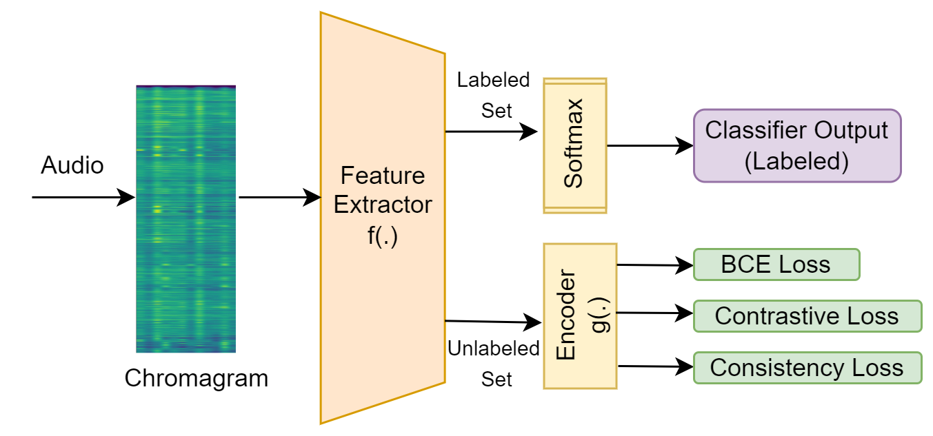
Figure 1: Block diagram of overall system

II-A Supervised Pre-training

For the 12 classes in $S^{l}$, we split the audio files into training, testing, and validation sets, then create 30-second chunks for all three sets. From now on, we will define these chunks as ‘audio samples’ and the master audio from which we extract chunks as ‘audio file’. We use PANNs model [21] to filter out any speech segments from these chunks, retaining only musical segments. We extract chromagram features and apply tonic normalization as described in [6]. A CNN-LSTM model is trained in a fully supervised manner on $S^{l}$ using categorical cross-entropy loss. for the 12 classes through cross-validation. This supervised CNN-LSTM model serves as a feature extractor $f(\cdot)$ by removing the final softmax layer, and is used to generate embeddings $y_{i}$ for both the labeled set $S^{l}$ and unlabeled set $S^{u}$.

II-B BCE Loss

For a pair of unlabeled audio samples $(z_{i}^{u},z_{j}^{u})$ drawn from the dataset $S^{u}$, we extract their corresponding feature representations $(y_{i}^{u},y_{j}^{u})$ using the feature extractor $f(.)$ and calculate the cosine similarity $\epsilon$ between them:

$$\varepsilon(y_{i}^{u},y_{j}^{u})=\frac{(y_{i}^{u})^{\top}y_{j}^{u}}{\|y_{i}^{u}\|\|y_{j}^{u}\|}$$

Subsequently, we assign the pairwise pseudo-label $t_{i,j}$as:

$$t_{i,j}=\mathbbm{1}{\left[\varepsilon(y_{i}^{u},y_{j}^{u})\geq\delta\right]},$$ (1)

where $\delta$ is a threshold that determines the minimum similarity required for two samples to be considered part of the same latent class. Apart from this, for all audio samples $z_{i}^{u}$ extracted from the same audio file, we assign $t_{i,j}=1$. The pairwise pseudo-label is then used to train the self-attention encoder model $g(.)$, which comprises a multi-head self-attention mechanism using scaled dot-product attention, along with layer normalization and feedforward sub-layers. We stack multiple such blocks to form $g(.)$, with the input being the normalised inner product of the outputs from the feature extractor $f(.)$: $p_{i,j}=(g(y_{i}^{u}))^{\top}g(y_{j}^{u})/\|g(y_{i}^{u})\|\cdot\|g(y_{j}^{u})\|$. The binary cross-entropy loss is defined as:

$$\ell_{bce}=t_{i,j}\log(p_{i,j})+(1-t_{i,j})\log(1-p_{i,j})$$ (2)

II-C Consistency Loss

Now, we define consistency loss, which ensures that the network produces similar predictions for an audio sample $z_{i}$ and its transformed version $\hat{z}_{i}$. In the context of our music data, the optimal transformation is pitch-shifting by $n$ notes, which should still represent the same Raga but at a higher pitch. To achieve this for our chromagram input, we shift the chromagram bins cyclically, creating 11 different transformations for each time-frame of the 12-dimensional chromagram. So, we apply mean squared error (MSE) loss between the embeddings $y_{i}=f(z_{i})$ and $\hat{y}_{i}=f(\hat{z}_{i})$ of the given input$z_{i}$ and its transformed version $\hat{z}_{i}$ to enforce consistency between the original and transformed inputs:

$$\ell_{mse}=\frac{1}{C_{l}}\sum_{i=1}^{C^{l}}\left(g(y_{i}^{l})-g(\hat{y}_{i}^{l})\right)^{2}+\frac{1}{C^{u}}\sum_{j=1}^{C^{u}}\left(g(y_{j}^{u})-g(\hat{y}_{j}^{u})\right)^{2}.$$ (3)

II-D Contrastive Learning

Given an input data point $z_{i}^{u}$ from the unlabeled set $S^{u}$, we first extract its embedding $y_{i}^{u}=f(z_{i}^{u})$ using the feature extractor $f(\cdot)$. For our contrastive loss, we need to generate appropriate positive and negative samples for each training point. For the negative samples, given each $z_{i}^{u}\in S^{u}$, the corresponding embedding $y_{i}^{u}\in S^{u}$ is compared against every other embedding $y_{n}\in S^{u}\cup S^{l}$ using cosine similarity $\varepsilon(y_{i}^{u},y_{n})$, such that $y_{i}^{u}\in S^{u}$ and $y_{n}\in S^{u}\cup S^{l}$. These similarities are ranked in ascending order, and the M=50 embeddings with the lowest similarity scores are selected as hard negatives.

$$\zeta_{i}^{u}=list(\varepsilon(y_{i}^{u},y_{n})),\forall\{y_{i}^{u}\in S^{u}\}$$

Now, for a given $y_{i}^{u}$, we can get negative samples by ranking the elements of $\zeta_{i}^{u}$ in ascending order and selecting the top M from the list. So, the set $\xi_{m}$ is given by:

$$\xi_{m}=\text{argtop}_{m}(\zeta_{i}^{u}),\forall i$$ (4)

For generating positive pairs, given an audio sample $z_{i}^{u}$, all other audio samples sourced from the same audio file are treated as positive pairs for the sample $z_{i}^{u}$ are surely supposed to be in the same class. For all such positive samples, their corresponding $\hat{y}_{i}^{u}\in\beta$ are treated as positive pairs in the loss function. The contrastive loss $\ell_{cl}$ is then defined as [10]:

$$\ell_{cl}(y_{i}^{u},\beta)=-\frac{1}{k}\sum_{\hat{y}_{i}^{u}\in\beta}\log\frac{e^{\varepsilon(y_{i}^{u},\hat{y}_{i}^{u})/\tau}}{e^{\varepsilon(y_{i}^{u},\hat{y}_{i}^{u})/\tau}+\sum_{\bar{y}\in\xi_{m}}e^{\varepsilon(y_{i}^{u},\bar{y}_{m}^{u})/\tau}}.$$ (5)

where $\tau$ is a temperature parameter that controls the concentration level of the distribution. The loss function encourages the embedding $y_{i}^{u}$ to be close to its positive pair $\hat{y}_{i}^{u}$ while pushing it away from the negatives $\bar{y}_{m}^{u}$.

The overall loss function for training the encoder model is a combination of the contrastive loss and the BCE loss:

$$\ell=\ell_{bce}+\beta\ell_{cl}+\gamma\ell_{mse}$$ (6)

By jointly optimizing this loss function, the model learns to accurately cluster embeddings, thereby improving the detection of novel Raga classes. While combining all 3 losses, we need to do proper scaling using $\beta$ and $\gamma$ hyper-parameters as the ranges of all 3 losses are very different.

II-E Evaluation

Given any set of embeddings $w_{i}$ obtained from $g(.)$, we apply clustering techniques to obtain predicted cluster labels:
Cosine Similarity: For all vectors $w_{i}=g(y_{i})$, we begin by calculating the cosine similarity $\epsilon$ between each pair of vectors, resulting in a cosine similarity matrix. Using this matrix, we define a threshold $th$, such that any pair of vectors with $\epsilon>th$ is assigned to the same cluster.
K-means: We use the output embeddings $w_{i}$ from the encoder model and apply the k-means algorithm to these 64-dimensional vectors to form clusters.
t-SNE and UMAP: We map the audio embeddings $w_{i}$ to a lower-dimensional space using t-SNE or UMAP, and then apply the k-means algorithm to cluster the reduced embeddings.

We evaluate clustering performance using metrics such as Silhouette Score (SS)[22], Davies-Bouldin Index (DBI)[23], and Calinski-Harabasz Index (CHI)[24] for label-independent assessments, and Adjusted Rand Index (ARI)[25] and Normalized Mutual Information (NMI)[26] to evaluate alignment with ground truth labels. We also compute Accuracy (ACC), for that, we first establish a one-to-one correspondence between the predicted clusters and the true clusters. For each true cluster $c^{t}$, we identify the predicted cluster $c^{p}$ that contains the maximum number of data points from $c^{t}$. The subset of data points in $c^{p}$ that also belong to $c^{t}$ is denoted by $c^{pt}$, defined as:

$$c^{pt}=\{w_{i}\mid w_{i}\in c^{p}\text{ and }w_{i}\in c^{t}\}.$$

The accuracy for the true cluster $c^{t}$ is then calculated as the ratio of the number of correctly assigned points in $c^{pt}$ to the total number of points in $c^{t}$:

$$\text{ACC}(c^{t})=\frac{|c^{pt}|}{|c^{t}|}\times 100.$$

Points that do not fall within these matched clusters are considered misclassifications. Additionally, if the same $c^{p}$ dominates more than one true cluster $c^{t}$, the clustering scheme is deemed invalid, and ACC, along with any other metric, is not computed.

TABLE I: Clustering Comparison for Unlabeled Classes: Baseline vs. Proposed Method

Metric	Cosine Similarity		t-SNE		UMAP		K-means
	Baseline	Proposed	Baseline	Proposed	Baseline	Proposed	Baseline	Proposed
SS	0.22	0.75	0.49	0.59	0.63	0.79	0.36	0.85
DBI	1.54	0.63	0.73	0.63	0.59	0.31	1.33	0.32
CHI	238.42	4739.47	3383.17	4601.59	8581.97	23033.67	861.76	11896.57
ARI	0.50	0.58	0.56	0.59	0.53	0.60	0.48	0.64
NMI	0.87	1.17	0.83	0.84	0.83	0.85	0.79	0.94
ACC (%)	58.96	72.10	71.98	73.11	71.48	72.99	70.75	79.34

TABLE II: Clustering Metrics for MERT, Melody extraction tool (Mel), and $f(\cdot)$ model (Cosine Similarity (C-sim), t-SNE, UMAP, K-means) for labeled data

Metric	MERT	Mel	C-sim.	t-SNE	UMAP	k-means
SS	0.13	-0.01	0.37	0.54	0.70	0.54
DBI	1.75	5.02	1.37	0.64	0.45	1.10
CHI	521	4.77	788.77	9577.83	26097.93	2884.15
ARI	-	-	0.74	0.72	0.76	0.83
NMI	-	-	1.93	1.89	1.90	1.99
ACC	-	-	81.87	85.51	83.88	90.05

III Experimental Results

For the unlabeled set $S^{u}$, we use a total of 51 audio files, corresponding to 2,435 audio samples and approximately 20.29 hours of data. The Raga class labels for $S^{u}$ are discarded, treating it as an unlabeled dataset. The labeled set $S^{l}$ comprises 141 audio files, segmented into 5,734 audio samples, totaling around 47.78 hours of data.

We initially train a CNN-LSTM model in a supervised manner for multi-class classification across 12 classes in the labeled set $S^{l}$. This model achieves an overall F-1 score of 0.89 through cross-validation and serves as the feature extractor for our baseline.

III-A Clustering on $S^{l}$

For audio samples in $S^{l}$, we first extract embeddings using the pre-trained MERT model [27], melody based embeddings from [28], and finally using the pre-trained CNN-LSTM feature extractor $f(\cdot)$, and cluster them using cosine-similarity as outlined in Section:II-E. The clustering results for the labeled dataset are shown in Table II. We observe that MERT and melody-based model produce very poor results even for label-independent metrics compared to $f(\cdot)$, so we discard them and use $f(\cdot)$ as feature extractor for our work.

III-B Results

For the baseline, we cluster the embeddings $y_{i}^{u}\in S^{u}$ obtained from the pre-trained model $f(\cdot)$ and show the results in tableI. In our proposed method, we utilize the output embeddings $g(y_{i}^{u})$ from the encoder model trained using a combined loss function, and we perform clustering in the same manner as with the labeled data. The clustering performance results are presented in Table I. As expected, the baseline results for $S^{u}$ are significantly worse than those for the labeled dataset. This outcome is anticipated since the feature extractor $f(\cdot)$ is not trained on $S^{u}$, and $S^{u}$ and $S^{l}$ contain disjoint Raga classes. Consequently, clustering performance is poor for both label-dependent and label-independent clustering metrics under the baseline.

However, our proposed method shows substantial improvement across nearly all metrics compared to the baseline. This improvement is also evident when visualizing the clusters using t-SNE for dimensionality reduction, followed by clustering with the proposed methods. The clusters produced by the baseline method appear significantly worse in contrast to the proposed method, which aligns with the lower performance metrics shown in the results Table I.

III-B1 Proposed Method vs. Baseline

The proposed method consistently outperforms the baseline across all metrics and clustering techniques. Particularly, we observe notable improvements in the SS, DBI, and CHI when using Cosine Similarity and K-means clustering techniques. This improvement in Cosine Similarity-based clustering can be attributed to the fact that our method inherently includes optimizations that encourage the model to learn embeddings that are better suited to cosine similarity. Specifically, during training, the loss function promotes the alignment of similar samples in the cosine similarity space.

As shown in Table I, the proposed method improves the SS for Cosine Similarity from 0.22 to 0.75, and reduces the DBI from 1.54 to 0.63. We also see a high increase in CHI, NMI, and ACC, indicating that the proposed method creates more distinct and well-separated clusters, resulting in better alignment with true labels and overall classification accuracy. Fig. 2 shows the confusion matrix for classification of 5 unknown Raga classes: Bhopali (Bh), Bageshri (Bg), Jog-Kouns (JK), Mishra-Khamaj (MK), and Puriya-Kalyan (PK). If we compute f1-scores based on the confusion matrix, we observe that the model performs well for Bageshri (F1: 0.85) and Bhopali (F1: 0.92), which are more distinct and straightforward Ragas. However, it struggles with Mishra-Khamaj (F1: 0.51), Jog-Kouns (F1: 0.69), and Puriya-Kalyan (F1: 0.60). These Ragas, being Mishra (mixed) Ragas, inherently share musical similarities with more than one Ragas in their structure itself, making them more challenging to distinguish and often leading to confusion for the model. This highlights the intrinsic complexity of Mishra Ragas and emphasizes the need for more refined approaches to accurately classify such Ragas.

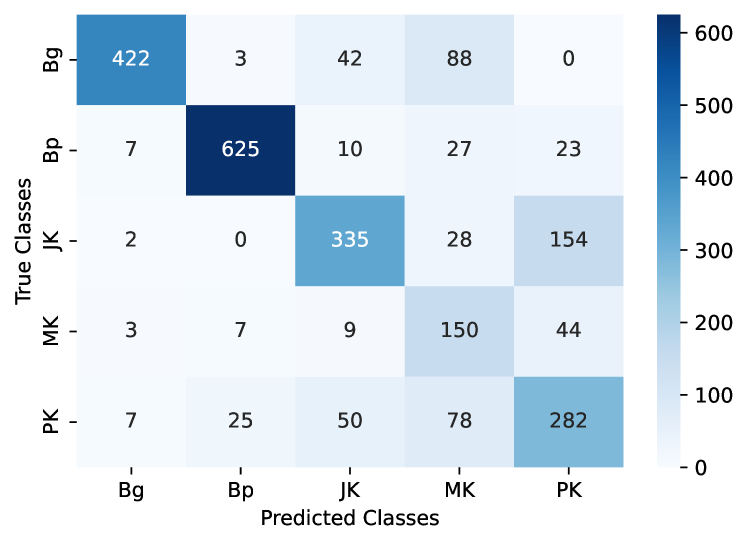
Figure 2: Confusion matrix for $S^{u}$

III-B2 Proposed Method vs. Labeled Data

The proposed method demonstrates strong clustering performance even without access to labeled data. For instance, in K-means clustering, the proposed method achieves a SS of 0.85 compared to 0.54 for labeled data, and it performs competitively with UMAP (0.79 vs. 0.70). Additionally, the proposed method achieves a lower DBI for UMAP (0.31 vs. 0.45) and significantly outperforms labeled data in Cosine Similarity-based clustering (0.63 vs. 1.37). These results indicate that the proposed method is a robust alternative in open-world scenarios where labeled data is scarce or unavailable.

III-B3 Clustering Quality and Scalability

The proposed method shows that the clusters hence obtained using the proposed method can approach or match the clustering quality of supervised methods. This is especially valuable in fields like MIR, particularly for the Raga Identification task, where labeled data is often limited. The ability to leverage large amounts of unlabeled data efficiently demonstrates the scalability of the method, making it a valuable contribution to tasks where manual labeling is infeasible or costly.

IV conclusion and future scope

In this study, we present a novel framework for open-set Raga classification in Indian Art music using Novel Class Discovery (NCD). By leveraging contrastive learning, our approach enables the model to effectively recognize and classify new, unseen Ragas that are not part of the training data. This framework addresses the challenge of limited labeled data in Music Information Retrieval (MIR), specifically in raga identification, by reducing the dependency on extensive manual labeling. It can also encourage the usage of thousands of hours of music data available on platforms like YouTube without the need for manual labeling.

In future work, we aim to extend our framework to improve the detection of both labeled and unlabeled classes, enhancing its capability to classify across a wider range of scenarios. By extending our framework to multimodal and hierarchical representation learning, we hope to enhance its flexibility and robustness, making it a valuable tool for the evolving field of MIR. Also, exploring better ways to handle Mishra Ragas can be a future direction for improvement.

References

- [1] X. Serra, “The computational study of a musical culture through its digital traces,” Acta Musicologica, vol. 89, no. 1, p. 24–44, Jun. 2017.
- [2] S. Chowdhuri, “Phononet: multi-stage deep neural networks for raga identification in hindustani classical music,” in ICMR, 2019.
- [3] S. Paschalidou and I. Miliaresi, “Multimodal Deep Learning Architecture for Hindustani Raga Classification,” Sensors & Transducers, vol. 261, no. 2, pp. 77–86, Feb. 2024.
- [4] A. A. Bidkar, R. S. Deshpande, and Y. H. Dandawate, “A north indian raga recognition using ensemble classifier,” IJEET, vol. 12, no. 6, pp. 251–258, 2021.
- [5] S. T. Madhusudhan and G. V. Chowdhary, “Deepsrgm - sequence classification and ranking in indian classical music via deep learning,” ArXiv, vol. abs/2402.10168, 2024. [Online]. Available: https://api.semanticscholar.org/CorpusID:208334841
- [6] P. Singh and V. Arora, “Explainable deep learning analysis for raga identification in indian art music,” 2024. [Online]. Available: https://arxiv.org/abs/2406.02443
- [7] A. Bendale and T. E. Boult, “Towards open set deep networks,” in 2016 IEEE Conference on Computer Vision and Pattern Recognition (CVPR), 2016, pp. 1563–1572.
- [8] Y. J. Lee and K. Grauman, “Object-graphs for context-aware category discovery,” in 2010 IEEE Computer Society Conference on Computer Vision and Pattern Recognition, 2010, pp. 1–8.
- [9] K. Han, S.-A. Rebuffi, S. Ehrhardt, A. Vedaldi, and A. Zisserman, “Automatically discovering and learning new visual categories with ranking statistics,” in International Conference on Learning Representations, 2020.
- [10] Z. Zhong, E. Fini, S. Roy, Z. Luo, E. Ricci, and N. Sebe, “Neighborhood contrastive learning for novel class discovery,” in 2021 IEEE/CVF Conference on Computer Vision and Pattern Recognition (CVPR), 2021, pp. 10 862–10 870.
- [11] K. Han, A. Vedaldi, and A. Zisserman, “Learning to discover novel visual categories via deep transfer clustering,” 2019 IEEE/CVF International Conference on Computer Vision (ICCV), pp. 8400–8408, 2019. [Online]. Available: https://api.semanticscholar.org/CorpusID:201646290
- [12] Y.-C. Hsu, Z. Lv, J. Schlosser, P. Odom, and Z. Kira, “Multi-class classification without multi-class labels,” in International Conference on Learning Representations, 2019. [Online]. Available: https://openreview.net/forum?id=SJzR2iRcK7
- [13] X. Yang, Z. Song, I. King, and Z. Xu, “A survey on deep semi-supervised learning,” IEEE Transactions on Knowledge and Data Engineering, vol. 35, no. 9, pp. 8934–8954, 2023.
- [14] Y. Yang, N. Jiang, Y. Xu, and D.-C. Zhan, “Robust semi-supervised learning by wisely leveraging open-set data,” IEEE Transactions on Pattern Analysis and Machine Intelligence, pp. 1–15, 2024.
- [15] Y. Xian, B. Schiele, and Z. Akata, “Zero-shot learning — the good, the bad and the ugly,” in 2017 IEEE Conference on Computer Vision and Pattern Recognition (CVPR), 2017, pp. 3077–3086.
- [16] Y. Xian, C. H. Lampert, B. Schiele, and Z. Akata, “Zero-shot learning—a comprehensive evaluation of the good, the bad and the ugly,” IEEE Transactions on Pattern Analysis and Machine Intelligence, vol. 41, no. 9, pp. 2251–2265, 2019.
- [17] A. N. Carr, Q. Berthet, M. Blondel, O. Teboul, and N. Zeghidour, “Self-supervised learning of audio representations from permutations with differentiable ranking,” IEEE Signal Processing Letters, vol. 28, pp. 708–712, 2021.
- [18] H. Yakura, K. Watanabe, and M. Goto, “Self-supervised contrastive learning for singing voices,” IEEE/ACM Transactions on Audio, Speech, and Language Processing, vol. 30, pp. 1614–1623, 2022.
- [19] H. Zhao, C. Zhang, B. Zhu, Z. Ma, and K. Zhang, “S3t: Self-supervised pre-training with swin transformer for music classification,” in ICASSP 2022 - 2022 IEEE International Conference on Acoustics, Speech and Signal Processing (ICASSP), 2022, pp. 606–610.
- [20] E. Fonseca, D. Ortego, K. McGuinness, N. E. O’Connor, and X. Serra, “Unsupervised contrastive learning of sound event representations,” in ICASSP 2021 - 2021 IEEE International Conference on Acoustics, Speech and Signal Processing (ICASSP), 2021, pp. 371–375.
- [21] Q. Kong, Y. Cao, T. Iqbal, Y. Wang, W. Wang, and M. D. Plumbley, “Panns: Large-scale pretrained audio neural networks for audio pattern recognition,” IEEE/ACM Transactions on Audio, Speech, and Language Processing, vol. 28, pp. 2880–2894, 2020.
- [22] P. J. Rousseeuw, “Silhouettes: A graphical aid to the interpretation and validation of cluster analysis,” Journal of Computational and Applied Mathematics, vol. 20, pp. 53–65, 1987.
- [23] D. L. Davies and D. W. Bouldin, “A cluster separation measure,” IEEE Transactions on Pattern Analysis and Machine Intelligence, vol. PAMI-1, no. 2, pp. 224–227, 1979.
- [24] T. Caliński and J. Harabasz, “A dendrite method for cluster analysis,” Communications in Statistics, vol. 3, no. 1, pp. 1–27, 1974.
- [25] N. X. Vinh, J. Epps, and J. Bailey, “Information theoretic measures for clusterings comparison: Variants, properties, normalization and correction for chance,” Journal of Machine Learning Research, vol. 11, no. 95, pp. 2837–2854, 2010. [Online]. Available: http://jmlr.org/papers/v11/vinh10a.html
- [26] A. Strehl and J. Ghosh, “Cluster ensembles - a knowledge reuse framework for combining multiple partitions,” Journal of Machine Learning Research, vol. 3, pp. 583–617, 01 2002.
- [27] Y. LI, R. Yuan, G. Zhang, Y. Ma, X. Chen, H. Yin, C. Xiao, C. Lin, A. Ragni, E. Benetos, N. Gyenge, R. Dannenberg, R. Liu, W. Chen, G. Xia, Y. Shi, W. Huang, Z. Wang, Y. Guo, and J. Fu, “MERT: Acoustic music understanding model with large-scale self-supervised training,” in The Twelfth International Conference on Learning Representations, 2024.
- [28] K. R. Saxena and V. Arora, “Interactive singing melody extraction based on active adaptation,” IEEE/ACM Transactions on Audio, Speech, and Language Processing, vol. 32, pp. 2729–2738, 2024.