Variability of hot sub-luminous stars and binaries: Machine learning analysis of Gaia DR3 multi-epoch photometry

Abstract

Context. Hot sub-luminous stars represent a population of stripped and evolved red giants located at the Extreme Horizontal Branch (EHB). Since they exhibit a wide range of variability due to pulsations or binary interactions, unveiling their intrinsic and extrinsic variability is crucial for understanding the physical processes responsible for their formation. In the Hertzsprung-Russell diagram, they overlap with interacting binaries such as Cataclysmic Variables (CVs).

Aims. By leveraging cutting-edge clustering algorithm tools, we investigate the variability of 1,576 hot subdwarf variable candidates using comprehensive data from Gaia DR3 multi-epoch photometry and Transiting Exoplanet Survey Satellite (TESS) observations.

Methods. We present a novel approach that utilises the t-distributed stochastic neighbor embedding (t-SNE) and the Uniform Manifold Approximation and Projection (UMAP) dimensionality reduction algorithms to facilitate the identification and classification of different populations of variable hot subdwarfs and Cataclysmic Variables in a large dataset. In addition to the publicly available Gaia time-series statistics table, we adopt extra statistical features that enhance the performance of the algorithms.

Results. The clustering results lead to the identification of 85 new hot subdwarf variables based on Gaia and TESS lightcurves and 108 new variables based on Gaia lightcurves alone, including reflection-effect systems, HW Vir, ellipsoidal variables, and high-amplitude pulsating variables. A significant number of known Cataclysmic Variables (140) distinctively cluster in the 2-D feature space among an additional 152 objects that we consider new Cataclysmic Variable candidates.

Conclusions. This study paves the way for more efficient and comprehensive analyses of stellar variability from both ground and space-based observations, as well as the application of machine learning classifications of variable star candidates in large surveys.

1 Introduction

Hot sub-luminous stars are hot and compact evolved low-mass stars located at the extreme horizontal branch, between the main sequence (MS) and the white dwarf (WD) sequence (Heber 2009, 2016). On a Hertzsprung-Russell diagram (HRD), they occupy the B and O spectral types, forming the population of hot subdwarf-B (sdB) and O (sdO) stars. A recent study on a 500 pc volume-limited sample of hot sub-luminous stars reports that they are dominated by the sdB population ($\sim 60\%$, Dawson et al. 2024), most of which are thought to have a canonical core mass of 0.47 $M_{\odot}$ and thin hydrogen layers ($\sim 10^{-4}-10^{-2}\,\rm M_{\odot}$; Saffer et al. 1994; Brassard et al. 2001). Their thin envelope mass suggests that sdBs are the remnant cores of low-mass red giant stars, stripped through binary interactions, introducing a different evolutionary path than for normal horizontal branch stars. This envelope mass does not allow them to support H-shell burning. After depletion of helium in the sdBs’ core, with a timescale of $\sim 10^{8}\,\rm yr$ (Dorman et al. 1993; Ostrowski et al. 2021), they first become sdOs and then evolve to the white dwarf cooling stage.

Evolutionary calculations show that sdB progenitors have likely undergone binary interactions (Han et al. 2002, 2003), including common envelope ejection (CEE, for short-period binaries with 0.1$-$10 day period), stable Roche Lobe Overflow (RLOF, for long period or composite binaries with 450$-$1600 day period, Vos et al. 2020), and mergers (e.g., He-WD + He-WD, Webbink 1984). Observational studies corroborate this (Pelisoli et al. 2020), where multiple studies have reported a significant fraction of hot subdwarfs in binary systems, either in close binaries with a main sequence or white dwarf companion (e.g., Geier et al. 2022; Schaffenroth et al. 2022, 2023), or in wide binaries with cool MS companions (e.g., Deca et al. 2012; Vos et al. 2019, 2020). This diversity makes them an excellent population for studying binary star evolution. In addition, a broad range of unseen companions have been confirmed to exist in hot subdwarfs, such as low-mass MS stars (dM), brown dwarfs, and white dwarf companions (Kupfer et al. 2015; Geier et al. 2010, 2022, 2023) through the Massive Unseen Companions to Hot Faint Underluminous Stars from SDSS (MUCHFUSS) project. The existence of these companions and their nature are often evidenced by the behaviour of the hot subdwarfs’ photometric lightcurves, such as ellipsoidal variability for white dwarf companions and reflection effects for low-mass companions (Schaffenroth et al. 2022; Barlow et al. 2022).

A population of hot subdwarfs has also been found to exhibit pulsations, which allow one to use asteroseismology to study their structure and evolution (e.g., Charpinet et al. 2010; Van Grootel et al. 2010; Reed et al. 2020; Sahoo et al. 2020; Silvotti et al. 2022; Krzesinski & Balona 2022; Uzundag et al. 2021, 2023, 2024). While the mechanism for exciting pulsations in subdwarfs is thought to be understood (i.e., the $\kappa$-mechanism operating on the Fe opacity bump; Charpinet et al. 1997; Fontaine et al. 2003), it is unclear why only a handful of subdwarfs are observed to pulsate, while most do not. Theoretical work has demonstrated that atomic diffusion is required, but it is unclear if other aspects, such as binary evolution history, also play a role (Hu et al. 2008, 2011; Bloemen et al. 2014).

It is essential to increase the detection of new variable hot subdwarfs to make a robust characterisation of their variability and improve our understanding of these stars. In addition to spectroscopic identifications of hot subdwarfs (e.g., Luo et al. 2019; Lei et al. 2020, 2023), which are often expensive to perform, previous efforts have been made to identify hot subdwarf candidates mainly based on their locations in the colour-magnitude diagram and proper-motion selection criteria (Geier et al. 2019; Geier 2020) using Gaia DR2 observations (Gaia Collaboration et al. 2018). Following similar steps, Culpan et al. (2022) compiled a large catalogue of more than 60,000 confirmed and candidate hot subdwarfs observed from Gaia EDR3 data (Gaia Collaboration et al. 2021a). Such selections are frequently affected by contamination from low-mass main-sequence stars, Cataclysmic Variables (CVs), and white dwarfs (Geier et al. 2019; Culpan et al. 2022; Barlow et al. 2022). Given this contamination, it is critical for target selections to develop an effective framework to separate hot subdwarfs from other populations of blue objects on the HR diagram and characterise their variability in multiple time-domain surveys.

There have been strong interests in developing machine learning algorithms to automate the variability search and characterisation of time-series data in time-domain astronomy (e.g.,Kim et al. 2021; Cui et al. 2022; Eyer et al. 2023; Monsalves et al. 2024) due to the growing volume of data generated by large surveys, such as the All Sky Automated Survey (ASAS, Pojmanski 2002), the Zwicky Transient Facility (ZTF, Bellm et al. 2019), and the Gaia mission (Gaia Collaboration et al. 2023). As the majority of these algorithms either depend on a particular survey (e.g., space- or ground-based) or are task-oriented (e.g., planet transit detection), their application is often limited to a certain number of specific cases and goals.

To that end, this paper delivers a machine learning framework for identifying variable hot subdwarfs and CVs from photometric time series alone. Our methods can be broadly applied to any photometric data, such as that from the BlackGEM (Groot et al. 2024), Gravitational-wave Optical Transient Observer (GOTO, Steeghs et al. 2022), and Legacy Survey of Space and Time (VRO/LSST, Ivezić et al. 2019) missions. The structure of this paper is as follows: In Section 2, data and methods are described. This is followed by feature engineering and cluster analysis in Section 3. Variability classification results are provided and discussed in Section 4. Conclusion and future prospects are presented in Section 5.

2 Data and Methods

2.1 Gaia observations

Precise astrometric and photometric measurements provided by Gaia significantly boost the identification of the population of hot subdwarf candidates in the colour-magnitude diagram. As such, Culpan et al. (2022) compiled a catalogue of 61,585 hot subdwarf candidates based on colour, absolute magnitude, and reduced proper motion selection criteria in Gaia EDR3 (Gaia Collaboration et al. 2021a), which serves as the basis of this work. The release of Gaia DR3 multi-epoch photometry (Eyer et al. 2023) allows us to cross-match this catalogue to find candidates with available lightcurves and further study their variability. This results in 2114 objects with available epoch photometry using the Gaia flag has_epoch_photometry=True. The remaining 59,471 were excluded from the analysis since they do not have available Gaia lightcurves.

Using the Gaia datalink service and the $astroquery.Gaia$ package (Ginsburg et al. 2019), we extracted the lightcurves of these objects across the three Gaia filter bands (G, BP, and RP bands). Before searching for periodicity, preliminary quality assessments were conducted. First, we retained objects with reliable parallax measurements (parallax_over_error ¿ 5). Second, the Gaia boolean quality flag reject_by_variability was used to remove data points rejected by the Gaia variability pipeline (Eyer et al. 2023), then objects with at least 25 observations in any of the three band lightcurves were selected, following the minimum number of observations suggested by Morales-Rueda et al. (2006) for detecting stellar variability. For the Gaia astrometric quality control, known as the re-normalised unit weight error (RUWE), RUWE$<$7 was adapted as a substantial amount of spectroscopically identified hot subdwarfs have been observed to exceed, up to RUWE=7, the recommended RUWE$<$1.4 limit, see Dawson et al. (2024) for more details. These selections result in 1,682 lightcurves ready for analysis. Typically, their Gaia G-band lightcurves have a median signal-to-noise ratio estimate (standard deviation of the magnitudes over root-mean-square (RMS) of the magnitude uncertainties) of 3.5 and a median number of observations of about 40, as well as a median magnitude of $\sim$15 mag.

2.2 Frequency analysis

The population of hot subdwarfs hosts diverse types of variability, including pulsating variables and eclipsing binaries, from close- to wide-binary systems. Therefore, their variability exhibits a wide range of both timescales, from minutes to months, and morphologies, from sharp eclipses to sinusoidal pulsations. Following the success of our frequency search algorithms in finding dominant frequencies in multi-band, heteroskedastic, and irregularly sampled lightcurves of hot subdwarf candidates from the MeerLICHT telescope (Ranaivomanana et al. 2023), we applied the same approach to search for periodicity in Gaia lightcurves. In brief, this method combines Fourier-based calculations, namely the generalised Lomb-Scargle periodogram, and phase dispersion measurements, known as Lafler-Kinman statistic, to alleviate the effects of noise and data gaps in a periodogram. This hybrid approach is referred to as the $\Psi-$static (Saha & Vivas 2017), where the notation $\Psi$ is used to represent the periodogram throughout this work.

Regarding the frequency grid search, the search was performed from zero up to 360 day^-1 according to the Nyquist-frequency of the 2-minute cadence of the Transiting Exoplanet Survey Satellite (TESS, Ricker et al. 2015) short-cadence observations, which were used to compare with the Gaia variability in Section 4. The frequency step is finely tuned, and is defined as the inverse of the total time base divided by an oversampling factor of 10, following results in the literature showing that this value is appropriate to ensure that no dominant frequency peaks are missed and to prevent a poor period estimation, which would occur if its value is taken too low (VanderPlas 2018; Schwarzenberg-Czerny 1996). In addition, the dominant frequency found is further optimised by fine tuning the frequency step with an oversampling factor of 100. This is only done on a small frequency window around the dominant frequency, where a frequency window size 10 times larger than the original frequency step is used on both side of the peak.

2.3 Uncertainties in the frequency estimates

The uncertainties in the dominant frequencies are estimated by adopting a Monte-Carlo approach, where the frequency algorithm is run 1000 times. The standard deviation of the dominant frequencies is taken as an estimate of the frequency uncertainty. Each iteration consists of: 1) drawing a sample from a normal distribution with zero mean and a width of the magnitude errors per observation; 2) creating a new lightcurve by adding the sample to the original lightcurve. Note that the magnitude errors in the original lightcurves are kept in the new lightcurves. 3) running the algorithm on the new lightcurve using the same fine tuned frequency window as in the frequency optimisation. Due to the finite sampling step in the frequency grid, each iteration could result in the same identified dominant frequency. To mitigate this, the frequency grids are shifted by 1/1000th of the frequency step for each of the 1000 iterations, ensuring that the frequency search is not confined to the same frequency peak in each iteration.

3 Feature engineering

3.1 Variability analysis

Once the dominant frequencies are computed for all candidates, a robust, unbiased method is required to determine the significance of the peaks and measure the reliability of the variability. Although the false alarm probability (FAP, Scargle 1982; Baluev 2008) is frequently used in the literature to measure the significance of the frequency peak, it is not well adapted to variables in the high frequency domain and in the case of signals with red noise (VanderPlas 2018). Additionally, the interpretation of the FAP becomes complex in our case, where two independent periodograms are combined in the hybrid approach. Therefore, we address this by exploring machine learning clustering algorithms to discriminate candidates with different significance levels and variability.

We explore various summary statistics that are capable of unveiling the fidelity of the frequency peaks and the variability of the Gaia time series. Extracting these parameters from the data is necessary in order to work with the clustering algorithms described in the next sections. First, we extracted the Gaia variability summary statistics table, which consists of statistical parameters (54 in total, excluding boolean parameters and object IDs) computed using the Gaia DR3 time series (Eyer et al. 2023). Second, after normalising the maximum amplitude in the $\Psi-$periodogram to one, we computed additional statistical features (24 features) specifically designed to help us define the significance of the peak, such as the 95th percentile of the amplitude for the 100 highest amplitude peaks, the 99th percentile of the amplitudes for the full spectrum, and the number of frequencies with amplitudes above 0.5. These features were found useful for distinguishing objects with clear variability as will be discussed in Section 3.2. We obtained 84 features in total (see Table LABEL:tab:all_features) when combining these features with the Gaia statistics table and other 6 parameters from the Gaia DR3 source database (Gaia Collaboration et al. 2023), such as BP$-$RP, parallax, and RUWE. Note that entries with missing values were removed from the table, leaving us with 1,576 final candidates out of the 1,682 objects.

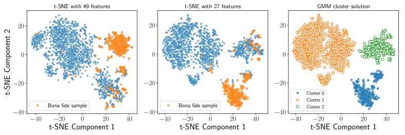
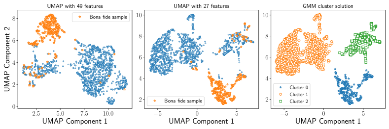
Figure 1: Clustering results using t-SNE (top panels) and UMAP (bottom panels) dimensionality reduction algorithms and clustering labels (right panels) from the Gaussian mixture model (GMM). The left and middle panels represent the 2-D components using 49 and 27 features, respectively. The orange open stars in these panels correspond to the manually selected objects with clear variabilities.

3.2 Dimensionality reduction

The next step is to transform these features into a lower-dimensional space such that we can visualise and identify possible clusters. This was done by applying dimensionality reduction techniques to our data, which convert high-dimensional features to a 2-D feature space. Dimensionality reduction is a common practice in machine learning and has been extensively used in astronomy to visualise and interpret data (Kao et al. 2024; Liao et al. 2024; Pantoja et al. 2022). Here, two non-linear dimensionality reduction techniques were explored: the t-distributed Stochastic Neighbor Embedding or t-SNE (van der Maaten & Hinton 2008) and the Uniform Manifold Approximation and Projection or UMAP (McInnes et al. 2018). These were chosen over other techniques (e.g., the Principal Component Analysis; PCA) due to their ability to find non-linear structures in data and their straightforward implementation.

Since we have more than 80 features, it is important to remove highly correlated features that could lead to noise in the visualisation (Kuhn & Johnson 2019). This also helps the algorithms, notably t-SNE, map the high-dimensional space to low-dimensional space efficiently. To identify correlated features, we calculate the Pearson correlation coefficient between all pair-wise combinations of features and excluded one feature from each pair in case of correlation values above 0.95. This reduces the number of features to 49, which is also recommended ($\sim$ 50) to efficiently optimise the t-SNE algorithm.

We further ranked the features using a Random Forest algorithm (Breiman 2001), which is a commonly used technique to obtain relative feature importance scores (e.g., Richards et al. 2012). The importance score of each feature is determined based on its ability to split the data into pure nodes (nodes with instances belonging to the same class) in the individual decision trees of the random forest model, see Breiman (2001) for more details. At this stage, the sole purpose is to obtain the feature scores. Therefore, the default Random Forest model hyper-parameters (e.g. the number of estimators) were used to fit the data. Upon model fitting, we obtained the relative importance scores of each feature. These scores will be used when optimising the t-SNE and UMAP algorithms in Sections 3.2.1 and 3.2.2.

We also manually labelled each object based on their phase-folded diagrams, where objects that exhibit an obvious variability are labelled as 0, while those with an ambiguous variability are labelled as 1. These labels were used when fitting the Random Forest algorithm. In addition, labelling the data allows us to examine the clustering performances and to visualise the physical or statistical distribution of each class (e.g., period distribution) in the clusters shown in Fig. 1, which we discuss further throughout the paper.

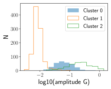
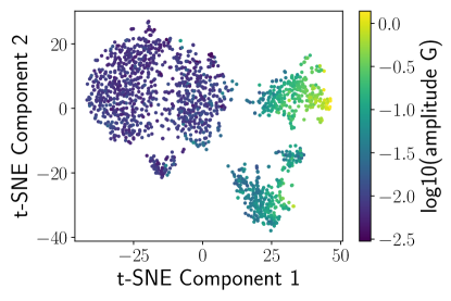
Figure 2: Amplitude distribution of each cluster in the Gaia G band (left panel) and gradient of the variability amplitude in the G-band across the t-SNE components (right panel).

3.2.1 Dimensionality reduction with t-SNE

In this work, the TSNE module from the scikit-learn python library was implemented (Pedregosa et al. 2011), where two crucial parameters, namely perplexity and learning rate, were optimised, while the other parameters are kept to their default values. The perplexity can be seen as a tuning parameter that measures the effective number of nearest neighbours to be considered when constructing the low-dimensional embedding. Before running the t-SNE algorithm, we first scaled each feature to have zero mean and unit standard deviation, which helps the algorithm to be more efficient in finding structures in the data. The optimised values of both parameters are: perplexity = 50 and learning rate = 600. With these settings and the 49 features, Fig. 1 shows the transformed low-dimensional projections, where we can identify three main clusters, namely Cluster 0, Cluster 1, and Cluster 2. These are discussed in more detail in Section 3.3. The orange open stars in the left and middle panels of Fig. 1 represent the objects we manually labelled, where most of them belong to one cluster. To label these clusters, we fit the two-dimensional projection data to a Gaussian mixture model (implemented in scikit-learn) with three mixture components. The advantage of using this model is that it provides the probability of each object to belong in a cluster. The quality of the class labels predicted by the Gaussian mixture model was evaluated using the so-called silhouette score (Rousseeuw 1987), in addition to visual inspection of the graphical output. This evaluation metric compares how well data points match their designated cluster to other clusters. We obtained a silhouette score of 0.535, which is generally considered to indicate a reasonable clustering solution (i.e. $>0.5$, Rousseeuw 1987). We further improved this by iteratively removing the least important features from the importance scores computed above, that might cause noise in the low-dimensional representation. In other words, we stopped the iterative process when no further improvements were visually detected in the output clusters and in the silhouette score. This results in 27 features with a silhouette score of 0.567. The t-SNE 2-D representation of this result is shown in Fig. 1, as well as the Gaussian mixture clustering solution. These 27 features are described in Table 3 and are used throughout the rest of the analysis.

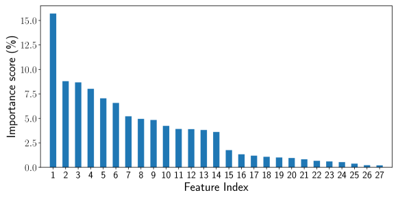
Figure 11: Random Forest feature importance scores for the 27 features listed in Table 4. The x-axis corresponds to the Feature ID in the table.

The most dominant features for the manually labelled objects include the 95th percentile of the first 100 frequency peaks, the number of peaks above 0.5 of the normalised $\Psi$ periodogram, and the 99th percentile of all periodogram peaks. However, these do not imply that these top features alone can explain the discrimination of the three clusters in the two-dimensional feature space; it only means that their importance scores are higher than the rest of the features, as shown in Figure 11. As previously mentioned, the aim of dimensionality reduction algorithms is to build new low-dimensional features from linear or non-linear combinations of high-dimensional features while preserving as much of the original information as possible. Since the low-dimensional features are mixtures of the original ones, we cannot conclude from the 2-D representation that a specific or a group of a few features are responsible for the distinction of the clusters.

3.2.2 Dimensionality reduction with UMAP

Similar to t-SNE, UMAP (McInnes et al. 2018) is a nonlinear algorithm for high-dimensional data visualisation, except that its dimensionality reduction approach is grounded in manifold theory and topological data analysis rather than probabilistic modeling as in t-SNE. The UMAP algorithm is implemented in the umap-learn python package (McInnes et al. 2018). We ran the UMAP algorithm with its default parameter values and the selected 27 features in Section 3.2.1, which already resulted in reasonable silhouette score values and distinctive visualisation (Fig. 1). The same features obtained from t-SNE were also used when running the UMAP algorithm to show that both algorithms output the same results using the same features, and to obtain meaningful clustering results. The obtained silhouette scores are very similar for the 27 features (0.597) and 49 features (0.599). Cluster labels were again obtained from the Gaussian mixture model. We identified three main clusters similar to those found with the t-SNE algorithm, which confirms the existence of these clusters in our data. The next section will compare the results from the two algorithms.

3.3 Cluster analysis and candidate selection

It is worth examining if the three clusters found by t-SNE and UMAP represent the same objects. Note that from the t-SNE and UMAP components, there are 290 and 297 objects in Cluster 0; 990 and 991 objects in Cluster 1; and 296 and 288 objects in Cluster 2, respectively. Therefore, we cross-matched the objects in the three clusters from both algorithms and found a total number of 1563/1576 matches ($\sim 99\%$): 289, 988, and 286 matches from Cluster 0, Cluster 1, and Cluster 2, repectively. Thus, we find strong consistency between the two clustering approaches. We examined the 13 mismatched objects, since the clustering results for t-SNE and UMAP match for 1,563 out of 1,576 objects. Of these 13 objects, 8 belong to Cluster 0 in UMAP and Cluster 2 in t-SNE. These objects exhibit large peak-to-peak magnitudes in the Gaia G band, with variations of at least 0.5 mag. In the 2-D t-SNE plot, they are located near the border of Cluster 2, close to Cluster 0, which may explain the mismatch in the cluster labels between UMAP and t-SNE for these objects. For the remaining 5 of the 13 objects, they appear either in Cluster 1 in UMAP and Cluster 2 in t-SNE, or vice versa, and are similarly positioned at the borders of each cluster. Aside from these cases, we did not observe any peculiar objects.

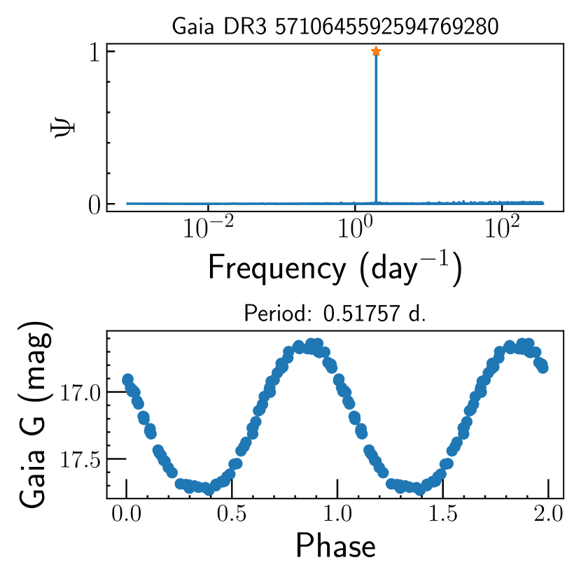
(a)

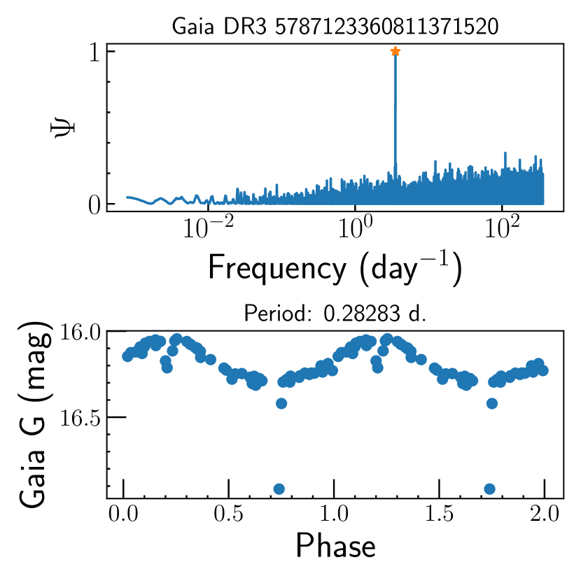
(b)

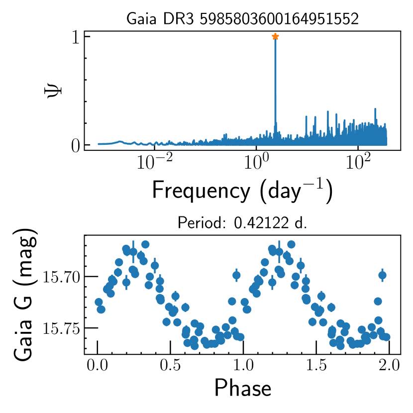
(c)

Three examples of objects (a,b,c) in Cluster 0.

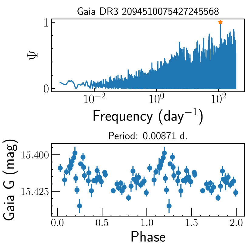
(d)

(e)

(f)

Three examples of objects (d,e,f) in Cluster 1.

(g)

(h)

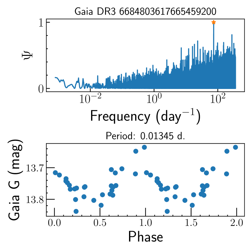
(i)

Three examples of objects (g,h,i) in Cluster 2.

Figure 10: Examples of periodograms and phase-folded lightcurves for each cluster. The top, middle, and bottom rows correspond to Cluster 0, Cluster 1, and Cluster 2, respectively.

As our primary goal is to identify objects with significant and clear variability among the clusters, we visually examined the lightcurves of the objects in each cluster. We observed that the three clusters reflect the clarity of the lightcurve variability, which can be translated to the lightcurve signal-to-noise ratio (SNR). More precisely, Cluster 1 contains objects with dubious variability that could be related to lightcurves with a relatively low SNR; Cluster 2 consists primarily of objects with ambiguous lightcurve shapes but high variability amplitudes; and Cluster 0 is dominated by objects with clear variability associated with high SNR lightcurves. Some examples of lightcurves in each cluster are shown in Fig. 10, where the top panels represent clear variables, typical for Cluster 0, the middle panels correspond to unclear variables found in Cluster 1, and the bottom panels consists of high amplitude ambiguous variables in Cluster 2. Since the two algorithms represent mostly the same objects per cluster, we focus our analysis on the clusters from the t-SNE components.

Furthermore, we measured the importance score of each of the 27 features using Random Forest based on the assigned label for each cluster, as we did with the manually labelled data. The results indicate that the amplitude of variability in the G band (amp_G) has the highest feature score, followed by the difference between the highest and lowest values of the G-band lightcurves (range_mag_g_fov), and the interquartile range of the G-band lightcurves (iqr_mag_g_fov). The rest of the features are listed according to their importance score in Table 4. As shown in the left panel of Fig. 2, the distribution of the amplitude in a log space reveals three distributions that support these results. In the same figure, a lower bound of the amplitude is seen at $\sim 20$ mmag for Cluster 0. Additionally, the right panel of Fig. 2 reveals that the amplitude values gradually increase from low to high values of the t-SNE component 1.

Based on the aforementioned results, we considered all objects in Cluster 0 (290 objects) as potential variable hot subdwarfs candidates and discuss their variability in Section 4.1, while objects in Cluster 2 are found to be mostly comprised of CVs and they are discussed in Section 4.2.

4 Results

4.1 Hot subdwarf variability classification

To confirm the nature of the variations found in the Gaia lightcurves, we compared them with those observed by TESS. First, we checked if any objects in the Gaia catalogue have lightcurves in TESS using the Lightkurve Python package (Lightkurve Collaboration et al. 2018). Second, we searched for fast (20 seconds) and short (2 minutes) cadence lightcurves and computed their Lomb-Scargle periodograms.

The periods found in the Gaia G band data are in strong agreement with those obtained by TESS for the objects in Cluster 0. For these objects, their variability types were thus determined with a high confidence. On the other hand, for objects without TESS observations, we could only provide a general classification, such as an eclipsing binary or a sinusoidal-like shape class. In order to ensure a homogeneous treatment of the whole sample, we did not rely on TESS data for frequency analysis results. Rather, we only used the TESS data to improve the fidelity of the classification. All lists of candidate classifications are provided in tables LABEL:tab:confirmed_hsd_cluster0$-$LABEL:tab:new_var_hsd_gaia.

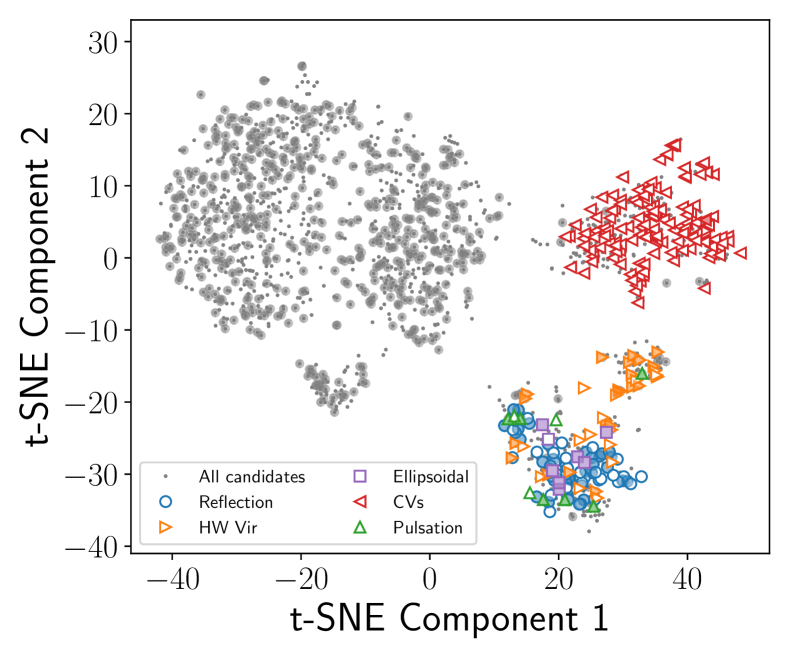
Figure 3: Identified variables from Gaia and TESS lightcurves, where shaded colours correspond to confirmed hot subdwarfs. CVs objects are obtained from the literature (See Section 4.2).

4.1.1 Variability of confirmed hot subdwarfs

We found 78 known variable hot subdwarfs amongst the 290 objects in Cluster 0 by cross-matching our data with a catalogue of spectroscopically identified hot subdwarfs and known variable hot subdwarfs from the literature (Schaffenroth et al. 2019, 2022, 2023; Culpan et al. 2022; Barlow et al. 2022; Lei et al. 2023; Dawson et al. 2024). Most of them (66/78) are identified from the compiled catalogue of 6,616 known hot subdwarfs Culpan et al. (2022), with 63/78 having short or fast cadence TESS lightcurves. Based on the Gaia and TESS lightcurves, we found 32 reflection-effect systems, 19 HW Vir systems, 6 pulsating variables, and 6 ellipsoidal variables. The remaining 15/78 systems are classified based solely on the Gaia three-band lightcurves, where we found 5 sinusoidal-like lightcurves, which could be associated with reflection-effect systems or ellipsoidal variations or a dominant pulsation mode, 5 eclipsing binaries, and 2 HW Vir systems. Fig. 5 shows examples of new HW Vir (TIC 129778070), reflection effect (TIC 333419799), and ellipsoidal variables (TIC 287977499) systems identified in this work.

4.1.2 Variability of hot subdwarfs candidates

From the non-confirmed hot subdwarfs (212/290), we identified 78 objects with short and/or fast cadence TESS lightcurves. Based on the Gaia and TESS lightcurves, we found 42 reflection-effect systems, 21 HW Vir systems, 3 pulsating variables, and 2 ellipsoidal variables. The remaining 134/212 hot subdwarf candidates were classified based on the Gaia three band lightcurves, where we found 60 sinusoidal-like lightcurves, 20 HW Vir systems, 14 eclipsing binaries, and 2 potentially pulsating variables. Thirty-eight objects have unclear variability, which prevents us from labelling them.

4.1.3 Pulsating hot subdwarfs

We identified a total of 9 already known pulsating variables from the known and candidate hot subdwarfs observed from Gaia and TESS. Three out of these nine are both pulsating in the Gaia and TESS lightcurves, namely TIC 273218137, TIC 53826859, and TIC 178626010 with a period of 0.09491 hr, 0.12096 hr, and 1.39841 hr, respectively. TIC 273218137 and TIC 53826859 are known pulsating hot subdwarfs from TESS observations (Krzesinski & Balona 2022), while TIC 178626010 is a new pulsating variable detected in this work and independently by Krzesinski et al. (in prep). In Fig. 6, their Gaia and TESS lightcurves are phased to the same periods and reference epochs $t_{0}$, using the short cadence lightcurves for TESS observations. The dominant frequencies found for these two objects are the same in the three Gaia bands. Therefore, they are potential candidates for mode identification from an amplitude ratio analysis (Aerts & Tkachenko 2023; Fritzewski et al. 2024). Their pulsation frequencies suggest that TIC 273218137 and TIC 53826859 are likely $p-$mode pulsators, and TIC 178626010 pulsates in the $g-$mode regime. The remaining six known pulsating variables have both low amplitude pulsations and higher amplitude orbital variability in their lightcurves. In our analysis, we were only able to detect their orbital variability in the Gaia data.

Table 1: Variability classification summary for known and candidate hot subdwarfs.

141/290 variable hot subdwarf candidates with Gaia and TESS lightcurves in Cluster 0
63 confirmed hot subdwarfs				78 hot subdwarf candidates
Confirmed Variables			New Variables	Confirmed Variables		New Variables		Total new
Reflection	15		17		2		40	57
HW Vir	13		6		7		14	20
Ellipsoidal	1		5		$-$		2	7
Pulsating variables	6		$-$		3		$1$	$1$
Others/Unclear	1		1		5		5	$-$
149/290 variable hot subdwarf candidates with only Gaia lightcurves in Cluster 0
	15 confirmed hot subdwarfs			134 hot subdwarf candidates				Total new
Sinusoidal		5			60			65
HW Vir		2			20			22
Eclipsing binary		5			14			19
Pulsating variables		$-$			2			2
Others/Unclear		3			38			$-$

4.1.4 Newly identified pulsating variables

We identified two unique high-amplitude pulsating objects from Gaia (Fig. 7): Gaia DR3 5835161264415038592 and Gaia DR3 5929109825689001856 with G-band peak-to-peak amplitudes of 0.21 mag and 0.25 mag, and pulsation periods of 0.38225 hr (22.935 min.) and 0.12844 hr (7.706 min.), respectively. The BP and RP periods for both objects are the same as those determined in the G band. Regarding their amplitudes in those bands, Gaia DR3 5835161264415038592 has peak-to-peak amplitudes of 0.21 mag and 0.19 mag in the BP and RP bands, respectively. Similarly, Gaia DR3 5929109825689001856 has peak-to-peak amplitudes of 0.29 mag and 0.23 mag, in the BP and RP bands, respectively. Their amplitude and frequency regimes suggest that these are candidate Blue Large Amplitude Pulsators (BLAPs, Pietrukowicz et al. 2017; Macfarlane et al. 2015).

4.2 Cataclysmic variables

Cluster 2 consists of 296 objects, from which 140 are known CVs (Barlow et al. 2022; Hou et al. 2023; Canbay et al. 2023) and 4 CV candidates from Krzesinski et al. (in prep). The remaining 152 objects are identified by SIMBAD as hot subdwarf candidates (70), Stars (61), Variables (9), and CV candidates (3). We consider all of these objects as CV candidates since all known objects in Cluster 2 are CVs with no contamination from other classes. The full lists of confirmed and candidate CVs are given in Table LABEL:tab:confirmed_cvs and LABEL:tab:candidate_cvs, respectively.

By cross-matching the objects in Cluster 2 with TESS, we found 127/140 confirmed CVs and 75/152 candidate CVs with TESS short cadence lightcurves. Their period distributions are shown in Fig. 8, where the periods are centered at 3.43 hr and 4.63 hr for the known and candidate CVs, respectively. The 127/140 CVs represent the same objects as in the (Canbay et al. 2023) catalogue. However, their reported periods are only available for 71 objects, mainly taken from Ritter & Kolb (2003), with a median period of 3.40 hr. Therefore, we add 56 new candidate orbital periods from our analysis.

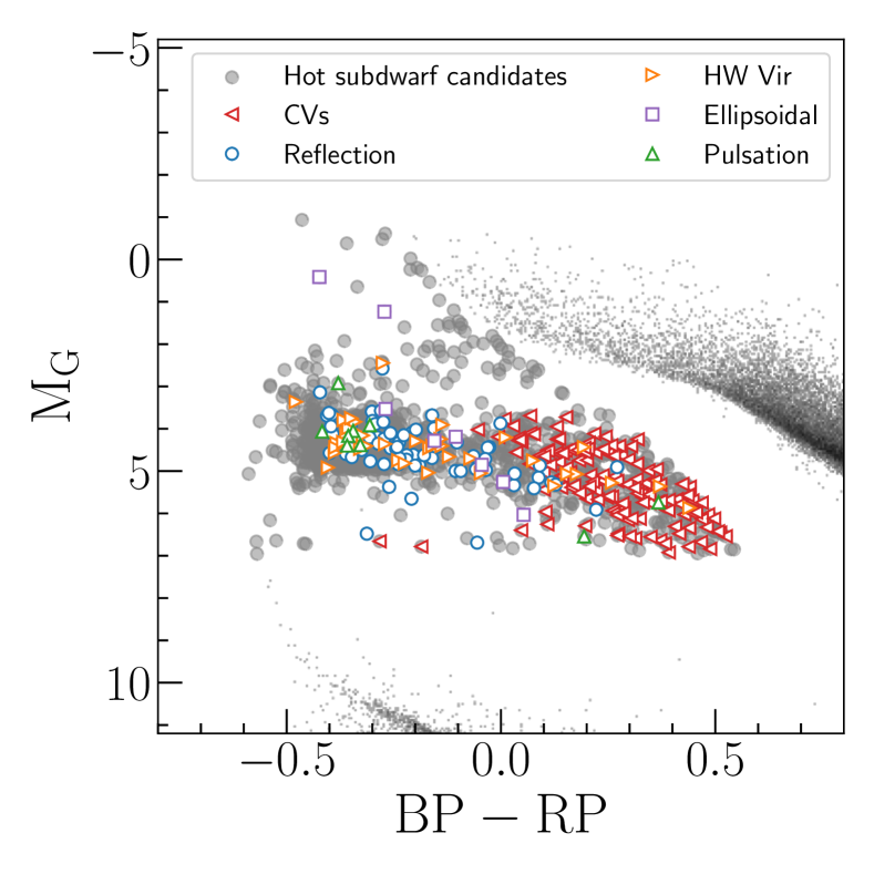
Figure 4: Gaia DR3 colour-magnitude diagram depicting the hot subdwarf candidates (1682) from Culpan et al. (2022) with Gaia lightcurves (grey circles). Variability classifications are shown for the selected variable hot subdwarf candidates (290) with TESS observations (141/290). Among the hot subdwarf candidates, Cataclysmic Variables (CVs) are also identified from literature and represented by left triangles. Grey background data points correspond to the Gaia Catalogue of Nearby Stars (Gaia Collaboration et al. 2021b).

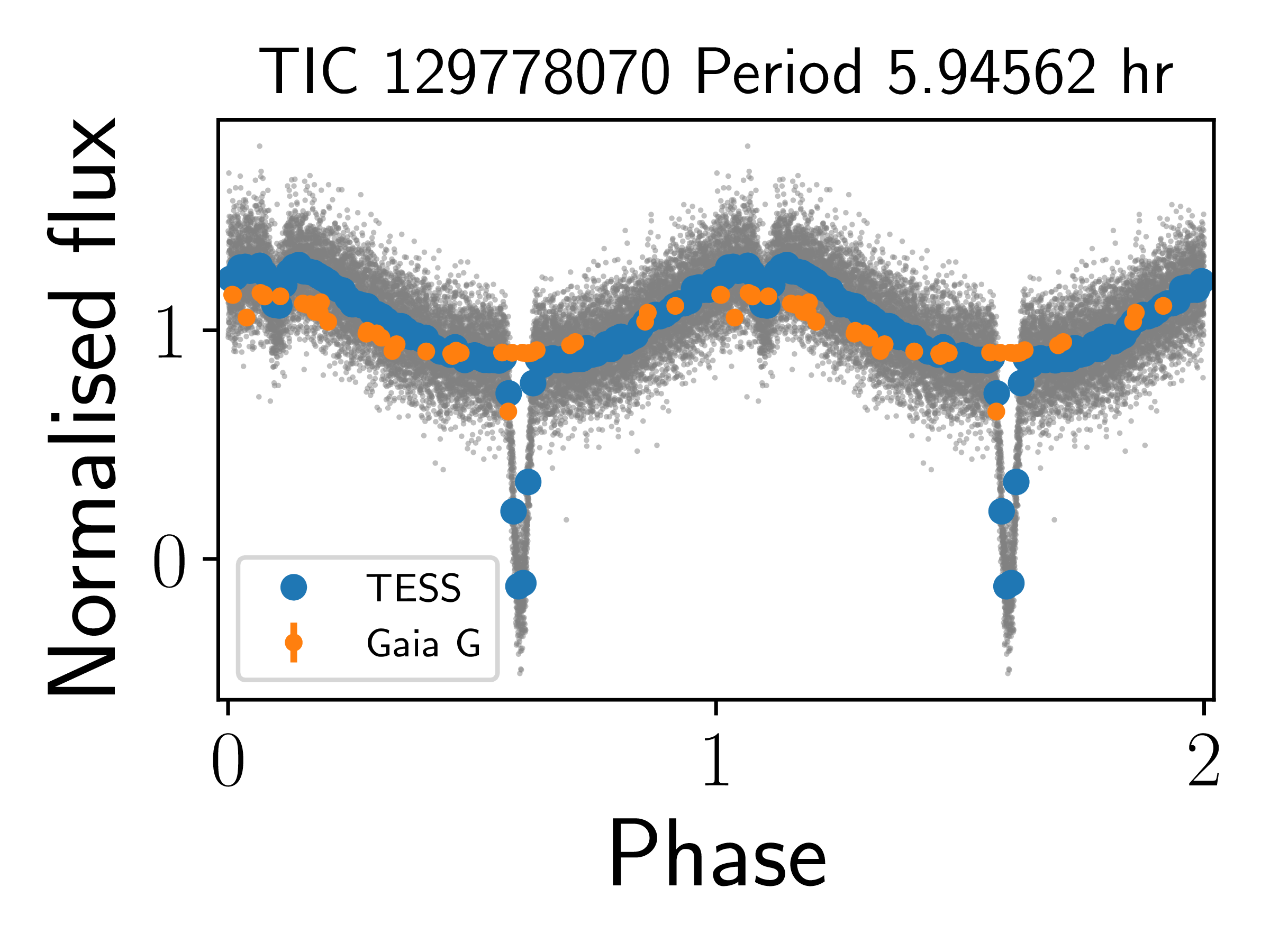
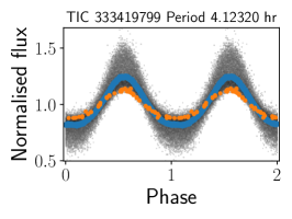
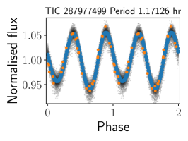
Figure 5: Three examples of new variable hot subdwarfs identified in this work. The lightcurves are phase-folded to the same periods and reference epochs. The three objects correspond to a HW Vir (left), a reflection effect (middle), and an ellipsoidal system (right). The lightcurves on the right are phased to twice the period to highlight the ellipsoidal variation. The blue lines represent the binned phase of the TESS lightcurves (grey data points), while the orange data points correspond to Gaia lightcurves.

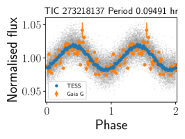
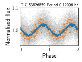
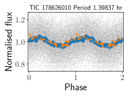
Figure 6: Three pulsating hot subdwarfs observed with Gaia and TESS. The left and middle panels correspond to known pulsating variables (Krzesinski & Balona 2022), and the right panel shows a pulsating variable identified in this work and Krzesinski et al (in prep.). The two lightcurves are folded to the same periods and reference epochs. The blue lines represent the binned phase of the TESS lightcurves (grey data points), while the orange data points correspond to Gaia lightcurves.

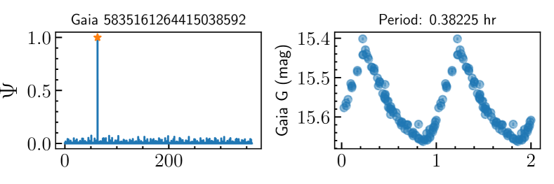
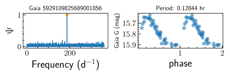
Figure 7: New high-amplitude pulsating variables observed with Gaia.

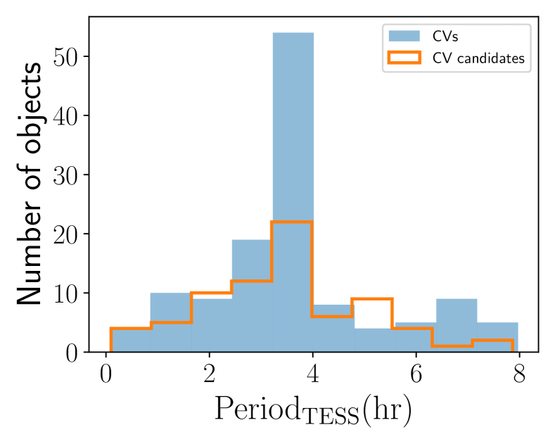
Figure 8: Period distribution of the confirmed and candidate CVs in Cluster 2.

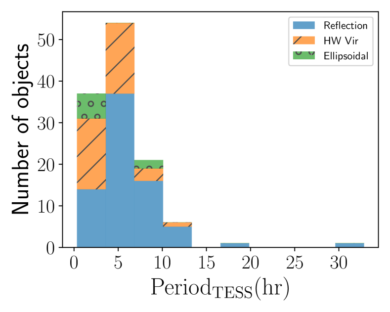
Figure 9: Period distribution of the binary systems observed with Gaia and TESS in Cluster 0.

4.3 Variability distributions

We have investigated the photometric variability of 290 and 296 objects in Cluster 0 and Cluster 2, respectively. A summary of the variability classification of confirmed and candidate hot subdwarfs is presented in Table 1. In Fig. 4, we present a Gaia colour-magnitude diagram of the 1,576 hot subdwarf variable candidates (grey circles) with the Gaia Catalogue of Nearby Stars in the background (grey data points, Gaia Collaboration et al. 2021b). Classified variables from Cluster 0 with TESS lightcurves are shown in the figure, where reflection systems are shown in blue open circle, HW Vir systems in orange right triangles, ellipsoidal variables in purple open squares, and pulsating variables in green triangles. Known CVs from the literature in Cluster 2 are represented in red left triangles. The lightcurve shapes of reflection-effect systems can be explained by the fact that the hot subdwarf irradiates and heats up one side of its cooler companion star, causing the cooler star to appear brighter on the side facing the hot subdwarf. As the system orbits, this creates a quasi-sinusoidal variability in the lightcurves. Depending on the viewing angle, reflection-effect systems can be eclipsing, forming the HW Vir systems. On the other hand, compact hot subdwarf binaries, particularly those with white dwarf companions, show ellipsoidal modulation in their lightcurves due to tidal distortion of the hot subdwarf, resulting in two maxima or two minima in their lightcurves. Examples of a reflection, HW Vir, and ellipsoidal system are shown in Fig.5. As previously introduced, the evolutionary stages of these systems can be understood through the lens of a binary evolution channel, notably a common envelope evolution for short-period systems. However, the exact formation mechanisms and evolutionary pathways are still areas of active research. On the other hand, CVs consist of a white dwarf primary and a mass-transferring secondary, typically a main sequence star. The shape of their lightcurves can be mostly explained by dramatic brightness increases known as outbursts, due to instabilities in the accretion disk, leading to sudden higher mass transfer. In Fig. 4, reflection-effect and HW Vir systems appear to occupy the same area (centered at $\rm M_{G}=4.4$ and $\rm BP-RP=-0.2$) and tend to be bluer than the known CVs (centered at $\rm M_{G}=5.3$ and $\rm BP-RP=0.3$).

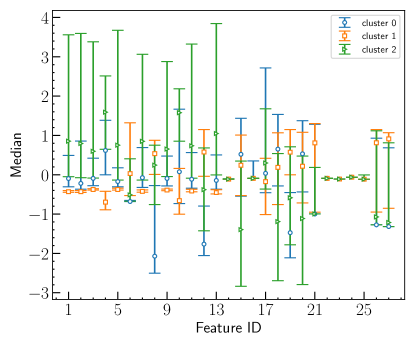
Figure 12: Distribution of the feature medians for each cluster. The x-axis corresponds to the feature ID listed in Table 4; The y-axis represents the median (open marker), the 10th percentile (lower cap), and the 90th percentile (upper cap) of each feature after a z-score normalisation.

Regarding their locations in the t-SNE components, HW Vir systems tend to be more concentrated in the sub-cluster between Cluster 0 and Cluster 2 as shown in Fig. 3, with a broader G-magnitude range (range_mag_g_fov around 0.50 mag) compared to the rest of the variables in Cluster 0 (range_mag_g_fov around 0.16 mag). Poor Gaia sampling of HW Vir systems could result in a sinusoidal-like shape of their lightcurves, as seen in the first panel of Fig. 5, due to the smearing effect. This could place them in a different position in Cluster 0 rather than in the sub-cluster. However, some HW Vir systems have shallower eclipse depths compared to others and this could also place them to the main cluster in Cluster 0. As previously mentioned, CVs lie in Cluster 2 with a G-magnitude range, range_mag_g_fov, centered at 1.15 mag. The distributions of the other features are presented in Fig. 12, with the 10th percentile, the median, and the 90th percentile of the features for each cluster. In comparison to the other two clusters, Cluster 2 exhibits a broader distribution of features, notably a high amplitude of variability, as seen in the right panel of Fig.2 and Fig. 12. Such differences in the feature distributions could be relevant for the reduction algorithms to well represent the clusters in the low-dimensional space.

As for the new variables identified from Gaia and TESS in Cluster 0, $\sim 23\%$ of them are classified as HW Vir systems, $\sim 67\%$ reflection-effect systems, and $\sim 10\%$ ellipsoidal and pulsating variables. With respect to their period distributions, Fig. 9 shows that the periods of both known and new HW Vir systems are in the range of $\sim 1.5$ hrs to $\sim 9$ hrs, while those of the reflection-effect systems range from $\sim 1.7$ hrs to $\sim 35$ hrs. This difference in the period distribution of the eclipsing reflection-effect (HW Vir) and non-eclipsing reflection-effect systems has also been observed in other studies. HW Vir systems tend to have shorter periods than non-eclipsing reflection-effect systems as found by (Schaffenroth et al. 2022). These authors have also found a broad peak at periods from 2 to 8 hrs, but could not find objects with a period longer than $\sim 30$ hrs for reflection-effect systems. They reported that periods longer than a few days might be scarce or not exist for such systems. However, we found several objects with periods longer than a few days from Gaia, which could be binary or eclipsing systems. Since we have no TESS observations for these objects, their variability types are referred to as sinusoidal or eclipsing binary.

5 Conclusion and future prospects

The present study set out to develop a generalisable machine learning algorithm that leverages multi-band photometric time series data in order to classify variable and non-variable subdwarfs. We developed our algorithm using multi-band time series photometry from Gaia and validated the algorithm using independent TESS data. Starting with a readily available catalogue of 61,585 hot subdwarf candidates, we were able to extract Gaia multi-band lightcurves of 1,682 objects with good astrometric solutions and a variable number of observations in the Gaia photometric bands (with a minimum of 25 observations). We searched for periodicities using the hybrid $\Psi-$statistic approach and estimated the uncertainties associated with the determined frequencies with a Monte-Carlo approach.

Using the sparsely sampled multi-band Gaia photometric data, we defined a number of bespoke summary statistics to supplement those already provided by the Gaia database. We applied machine learning algorithms to both calculate feature importance and perform dimensionality reduction, before applying a clustering algorithm that identified three clusters, which are predominantly predicted by the amplitude of the photometric variability in the Gaia G band. We further validated the results by applying two different dimensionality reduction techniques which resulted in 99% similar results.

The three clusters that we identified correspond to (candidate) hot subdwarfs with statistically significant variability (cluster 0), non-variable subwarfs (cluster 1), and Cataclysmic Variables (cluster 2).

Upon further inspection, we were able to identify different populations of variable hot subdwarfs observed from Gaia and TESS in Cluster 0. A significant number of them are in binaries, while a few pulsating variables are detected. The scarcity of the observed pulsating variables in Gaia could be explained by the fact that hot subdwarfs pulsate with low-amplitude light variations in the order of a few milli-mag.

Our analysis allowed us to newly identify a large number stars as variables, notably reflection-effect and HW Vir systems. The key findings of the clustering analysis are summarised as follows:

• In Cluster 0, 89 new hot subdwarf variables were identified from Gaia and TESS observations, while 108 new variables are found from Gaia alone. These new variables are mainly reflection-effect and HW Vir systems.

• In the same Cluster 0, 9 previously identified pulsating variables are found among the variable hot subdwarf candidates. We further identify two new high amplitude pulsating objects that are consistent with being BLAPs.

• In Cluster 2, a large number of CVs are identified, where 140 are spectroscopically confirmed in other studies. We consider the remaining 156 objects in cluster 2 to be CV candidates.

• Feature evaluation based on the three clusters shows that features related to the photometric variations in the G band have high contributions in characterising the clusters, including the amplitude, the magnitude range, and the interquartile range of the G-band lightcurves. The G-band amplitude distribution suggests a lower limit of $\sim 0.02$ mag on the detection of clear variability in the lightcurve.

The classification algorithm developed in this work was specifically designed to be flexible and generalisable. We used widely available features and developed new features that can be efficiently calculated for independent data sets with different properties. As a result of this, we can include new observations and objects without having to retrain the algorithm. Furthermore, our results can be used to help build labelled datasets for future supervised machine learning classifications of variable stars.

Scientifically, our results are twofold. First, we have developed a robust method for identifying variable subdwarf stars. Second, we have developed an algorithm that efficiently identifies CVs without the need for expensive follow-up spectroscopic observations. Together, these results allow us to confidently identify new variable subdwarfs for further analysis from existing data while filtering out contaminating sources such as CVs. While hundreds of hot subdwarfs and CVs have already been discovered, a systematically discovered sample of these objects is required to better understand various binary interaction processes, such as mass transfer, common envelope evolution, and tidal interactions. Furthermore, having an algorithm that efficiently identifies variable and non-variable subdwarfs from sparsely sampled data with known amplitude biases offers a unique opportunity towards building observational instability strips. By increasing the number of known sdBVs, we can perform population-level asteroseismic studies, similar to the work done for $\beta$ Cep stars using Gaia and TESS data (Fritzewski et al. 2024). This approach has the potential to reveal new insights into the pulsation properties and interior structure of hot subdwarfs by leveraging multi-colour photometry and observational amplitude ratios for mode identifications.

Spectroscopic follow-up observations, such as those with the 4-metre Multi-Object Spectroscopic Telescope (4MOST,de Jong et al. 2019), William Herschel Telescope Enhanced Area Velocity Explorer (WEAVE, Jin et al. 2024), Sloan Digital Sky Survey V (SDSS-V, Kollmeier et al. 2019), and LAMOST (Cui et al. 2012), may deliver radial-velocity data and atmospheric parameters to confirm the physical nature of these new variables (153 hot subdwarf candidates and 152 cataclysmic variable candidates), as well as the two new high-amplitude pulsating variables identified from Gaia. Other future prospects include photometric observations of the pulsating variables identified in this work using BlackGEM (Groot et al. 2024) to obtain multi-band pulsation amplitudes for mode identifications and asteroseismic modelling. Additionally, the release of Gaia Data Release 4 (DR4), which will include all photometric data, offers a valuable prospect for further exploration. Once the complete photometric dataset becomes available, this work can be immediately applied to the remaining 59 471 objects, enabling a comprehensive analysis of variability across a wider range of sources.

Appendix A Appendix

Table 2: List of all 84 features used in the feature selection. Features marked with (*) were computed in this work, those with ($\nmid$) are from the Gaia DR3 source database (Gaia Collaboration et al. 2023), while the rest were obtained from the Gaia variability summary table (Eyer et al. 2023). A full description of these Gaia statistics can be found in the Gaia documentation here.

No.	Feature	Description
		Selected features for the clustering analysis
1	log_sigvar*	Significance of variability in the G band in a log scale
2	frac_period*	Period over the standard deviation (std) of the three band Gaia lightcurve periods
3	std*	Standard deviation of the G, BP, and RP periods
4	fapG*	False alarm probability of the lomb-scargle dominant frequency peak (G band)
5	fapRP*	False alarm probability of the lomb-scargle dominant frequency peak (RP band)
6	fapBP*	False alarm probability of the lomb-scargle dominant frequency peak (BP band)
7	Period_G*	Derived period from the G-band lightcurve
8	Period_BP*	Derived period in the BP-band lightcurve
9	period_RP*	Derived period in the RP-band lightcurve
10	amp_G*	Amplitude of variability in the G band (mag.)
11	amp_BP*	Amplitude of variability in the BP band (mag.)
12	kurtosisG*	G-band kurtosis of the periodogram
13	p99*	99th percentile of all periodogram peaks based on the G-band lightcurves
14	p95_100*	95th percentile of the first 100 frequency peaks based on the G-band lightcurves
15	n05*	Number of peaks above 0.5 of the normalised $\Psi-$ periodogram based on the G band
16	psi_sigvar*	G-band median absolute deviation of the periodogram
17	bp_rp $\nmid$	BP$-$RP colour
18	range_mag_g_fov	The range of the G-band time series
19	abbe_mag_g_fov	The Abbe value of the G-band time series
20	iqr_mag_g_fov	The Interquartile Range (IQR) of the G-band time series
21	mad_mag_g_fov	The Median Absolute Deviation (MAD) of the G-band time series
22	stetson_mag_g_fov	The single-band Stetson variability index
23	abbe_mag_bp	The Abbe value of the BP-band time series
24	abbe_mag_rp	The Abbe value of the RP-band time series
25	outlier_median_g_fov	Greatest absolute deviation from the G median normalized by the error
26	skewness_mag_bp	The standardised unbiased unweighted skewness of the BP-band time series
27	std_dev_over_rms_err_mag_g_fov	Signal-to-Noise G estimate
		Excluded features in the feature selection processes
28	G_abs*	Gaia G absolute magnitude
29	N_G*	Number of observations in the G band.
30	N_BP*	Number of observations in the BP band
31	N_RP*	Number of observations in the RP band.
32	amp_RP*	Amplitude of variability in the RP band (mag.)
33	p90_100*	90th percentile of the first 100 frequency peaks
34	p99_100*	99th percentile of the first 100 frequency peaks
35	rmse_over_ptp_amp*	Root mean square error (RMSE) of the Lomb-Scargle model
		fit over the peak-to-peak G amplitude
36	parallax $\nmid$	Gaia parallax
37	parallax_error $\nmid$	Gaia parallax error
38	phot_g_mean_mag $\nmid$	G-band mean magnitude
39	phot_g_n_obs $\nmid$	Number of observation contributing to G photometry
40	RUWE $\nmid$	Renormalised unit weight error
41	num_selected_g_fov	Total number of G FOV transits selected for variability analysis
42	mean_obs_time_g_fov	Mean observation time for G observations
43	time_duration_g_fov	Time duration of the G time series
44	min_mag_g_fov	The minimum value of the G-band time series
45	max_mag_g_fov	The maximum value of the G-band time series
46	mean_mag_g_fov	The mean of the G-band time series
47	median_mag_g_fov	The median of the G-band time series
48	trimmed_range_mag_g_fov	Trimmed difference between the highest and lowest G-band time series
49	std_dev_mag_g_fov	Square root of the unweighted G magnitude variance
50	skewness_mag_g_fov	The standardised unbiased unweighted skewness of the G-band time series
51	kurtosis_mag_g_fov	The standardised unbiased unweighted kurtosis of the G-band time series
52	num_selected_bp	Total number of BP observations selected for variability analysis
53	mean_obs_time_bp	Mean observation time for BP observations
54	time_duration_bp	Time duration of the BP time series
55	min_mag_bp	The minimum value of the BP-band time series
56	max_mag_bp	The maximum value of the BP-band time series
57	mean_mag_bp	The mean of the BP-band time series
58	median_mag_bp	The median of the BP-band time series
59	range_mag_bp	The range of the BP-band time series
60	trimmed_range_mag_bp	Trimmed difference between the highest and lowest BP-band time series
61	std_dev_mag_bp	Square root of the unweighted BP magnitude variance
62	kurtosis_mag_bp	The standardised unbiased unweighted kurtosis of the BP-band time series
63	mad_mag_bp	The Median Absolute Deviation (MAD) of the BP-band time series
64	iqr_mag_bp	The Interquartile Range (IQR) of the BP-band time series
65	stetson_mag_bp	The single-band Stetson variability index
66	std_dev_over_rms_err_mag_bp	Signal-to-Noise BP estimate
67	outlier_median_bp	Greatest absolute deviation from the BP median normalized by the error
68	num_selected_rp	Total number of RP observations selected for variability analysis
69	mean_obs_time_rp	Mean observation time for RP observations
70	time_duration_rp	Time duration of the RP time series
71	min_mag_rp	The minimum value of the RP-band time series
72	max_mag_rp	The maximum value of the RP-band time series
73	mean_mag_rp	The mean of the RP-band time series
74	median_mag_rp	The median of the RP-band time series
75	range_mag_rp	The range of the RP-band time series
76	trimmed_range_mag_rp	Trimmed difference between the highest and lowest RP-band time series
77	std_dev_mag_rp	Square root of the unweighted RP magnitude variance
78	skewness_mag_rp	The standardised unbiased unweighted skewness of the RP-band time series
79	kurtosis_mag_rp	The standardised unbiased unweighted kurtosis of the RP-band time series
80	mad_mag_rp	The Median Absolute Deviation (MAD) of the RP-band time series
81	iqr_mag_rp	The Interquartile Range (IQR) of the RP-band time series
82	stetson_mag_rp	The single-band Stetson variability index
83	std_dev_over_rms_err_mag_rp	Signal-to-Noise RP estimate
84	outlier_median_rp	Greatest absolute deviation from the RP median normalized by the error

Table 3: Feature ranking based on the manual labelling. Features marked with (*) were computed in this work, those with ($\nmid$) are from the Gaia DR3 source database (Gaia Collaboration et al. 2023), while the rest were obtained from the Gaia variability summary table

(Eyer et al. 2023) ID Feature Description 1 p95_100* 95th percentile of the first 100 frequency peaks based on the G-band lightcurves 2 n05* Number of peaks above 0.5 of the normalised $\Psi$ periodogram based on the G band 3 p99* 99th percentile of all periodogram peaks based on the G-band lightcurves 4 Period_G* Derived period from the G-band lightcurve 5 frac_period* Period over the standard deviation (std) of the three band Gaia lightcurve periods 6 fapG* False alarm probability of the lomb-scargle dominant frequency peak (G band) 7 psi_sigvar* G-band median absolute deviation of the periodogram 8 kurtosisG* G-band kurtosis of the periodogram 9 iqr_mag_g_fov he Interquartile Range (IQR) of the G-band time series 10 std* Standard deviation of the G, BP, and RP periods 11 amp_G* Amplitude of variability in the G band (mag.) 12 log_sigvar* Significance of variability in the G band in a log scale 13 mad_mag_g_fov The Median Absolute Deviation (MAD) of the G-band time series 14 range_mag_g_fov The range of the G-band time series 15 abbe_mag_bp The Abbe value of the BP-band time series 16 abbe_mag_rp The Abbe value of the RP-band time series 17 Period_RP* Derived period from the RP-band lightcurve 18 fapBP* False alarm probability of the lomb-scargle dominant frequency peak (BP band) 19 abbe_mag_g_fov The Abbe value of the G-band time series 20 stetson_mag_g_fov Stetson G FoV variability index 21 Period_BP* Derived period from the BP-band lightcurve 22 amp_BP* Amplitude of variability in the BP band(mag.) 23 fapRP* False alarm probability of the lomb-scargle dominant frequency peak (RP band) 24 std_dev_over_rms_err_mag_g_fov Signal-to-Noise G FoV estimate 25 bp_rp $\nmid$ BP $-$ RP colour 26 outlier_median_g_fov The most outlying measurement with respect to the median 27 skewness_mag_bp The standardised unbiased unweighted skewness of the BP-band time series

Table 4: Feature ranking based on the three cluster labels. Features marked with (*) were computed in this work, those with ($\nmid$) are from the Gaia DR3 source database (Gaia Collaboration et al. 2023), while the rest were obtained from the Gaia variability summary table (Eyer et al. 2023)

ID	Feature	Description
1	amp_G*	Amplitude of variability in the G band (mag.)
2	range_mag_g_fov	The range of the G-band time series
3	iqr_mag_g_fov	he Interquartile Range (IQR) of the G-band time series
4	log_sigvar*	Significance of variability in the G band in a log scale
5	stetson_mag_g_fov	Stetson G FoV variability index
6	n05*	Number of peaks above 0.5 of the normalised $\Psi$ periodogram based on the G band
7	std_dev_over_rms_err_mag_g_fov	Signal-to-Noise G FoV estimate
8	p95_100*	95th percentile of the first 100 frequency peaks based on the G-band lightcurves
9	mad_mag_g_fov	The Median Absolute Deviation (MAD) of the G-band time series
10	bp_rp $\nmid$	BP $-$ RP colour
11	outlier_median_g_fov	The most outlying measurement with respect to the median
12	p99*	99th percentile of all periodogram peaks based on the G-band lightcurves
13	amp_BP*	Amplitude of variability in the BP band(mag.)
14	Period_G*	Derived period from the G-band lightcurve
15	abbe_mag_g_fov	The Abbe value of the G-band time series
16	kurtosisG*	G-band kurtosis of the periodogram
17	skewness_mag_bp	The standardised unbiased unweighted skewness of the BP-band time series
18	abbe_mag_bp	The Abbe value of the BP-band time series
19	psi_sigvar*	G-band median absolute deviation of the periodogram
20	abbe_mag_rp	The Abbe value of the RP-band time series
21	fapG*	False alarm probability of the lomb-scargle dominant frequency peak (G band)
22	Period_RP*	Derived period from the RP-band lightcurve
23	Period_BP*	Derived period from the BP-band lightcurve
24	frac_period*	Period over the standard deviation (std) of the three band Gaia lightcurve periods
25	std*	Standard deviation of the G, BP, and RP periods
26	fapRP*	False alarm probability of the lomb-scargle dominant frequency peak (RP band)
27	fapBP*	False alarm probability of the lomb-scargle dominant frequency peak (BP band)

Table 5: Variability of 63 confirmed hot subdwarfs identified from Gaia and TESS. Object types marked with (*) appear to have high-frequency pulsations in addition to their binarity. The columns $\rm dP_{Gband}$ and $\rm dP_{TESS}$ represent the uncertainties in the Gaia G and TESS periods, respectively. New variables identified in this work are referenced as ”this work” (TW).

Gaia DR3 ID	RA	DEC	$\rm Period_{Gband}$	$\rm dP_{Gband}$	$\rm Period_{TESS}$	$\rm dP_{TESS}$	Type	Ref
	[deg]	[deg]	[hr]	$\rm[hr]\times 100$	[hr]	$\rm[hr]\times 100$
5790285036556643072	210.48072	-75.22608	3.156741	0.000521	3.156749	0.000019	HW Vir	[1]
5216785445160303744	132.06451	-74.31507	1.171261	0.000127	1.171255	0.000037	Ellipsoidal	[TW]
4657996005080302720	82.91801	-69.88371	6.276955	0.000684	6.277055	0.000708	HW Vir	[TW]
6429036528482072576	305.71363	-65.42238	14.371672	0.022317	14.371522	0.000433	Pulsation	[2]
5864200981429024000	203.70778	-64.14217	3.54739	0.000153	3.547349	0.000237	HW Vir*	[TW]
5495360631749769600	95.16056	-57.09387	6.007468	0.001789	6.007267	0.002919	Reflection	[TW]
4929394649214080896	23.05287	-49.56128	10.173414	0.003073	10.173537	0.000271	Reflection	[TW]
5362804330246457344	163.66888	-48.78408	8.570661	0.001852	8.570712	0.000117	Reflection	[TW]
6527251469785220352	347.43049	-47.75821	6.338511	0.005961	6.338450	0.000236	HW Vir*	[TW]
6674565274623506560	308.95701	-46.62934	0.074241	0.000007	11.113793	0.000913	HW Vir	[TW]
4042163871810793600	271.12932	-34.32882	2.328577	0.000473	2.328570	0.000042	HW Vir	[TW]
6613267462718776832	331.46679	-31.68444	8.197466	0.010398	8.197268	0.000053	Reflection	[TW]
5031702144593331712	12.9072	-30.71547	5.82758	0.004099	5.827558	0.000120	Reflection	[TW]
6785706005902423680	325.48686	-29.27522	10.091575	0.002768	10.092037	0.000142	Reflection	[TW]
5642627428172192640	133.30232	-28.76838	3.042105	0.001485	3.042133	0.000011	Ellipsoidal	[TW]
5468670738602933504	156.73529	-27.38255	2.844166	0.000968	2.844192	0.000015	HW Vir	[3]
5661504084315014656	143.70102	-25.21241	3.429692	0.004651	3.429681	0.000032	Reflection	[TW]
2961366588952039552	79.52903	-23.14588	2.18813	0.000113	2.188130	0.000048	HW Vir*	[1]
5619750198969385856	109.91911	-21.88953	3.452925	0.000658	3.452910	0.000019	Reflection	[TW]
6196248648201755904	200.31517	-21.45491	11.699907	0.012550	11.699882	0.001054	Pulsation	[2]
5109790010155109760	59.09717	-15.15539	5.205322	0.009554	5.205502	0.000107	Reflection	[TW]
3675067076961979264	191.08437	-8.67142	2.801261	0.000196	2.801302	0.000396	Pulsation	[2]
5753841281270433536	129.05426	-8.03995	2.132835	0.000083	2.132840	0.000042	HW Vir*	[1]
4245906369913936000	305.00195	4.63237	2.648959	0.000091	2.648989	0.000017	HW Vir	[3]
1735991253803944960	311.58663	6.44034	7.237559	0.007191	7.239854	0.000086	Ellipsoidal	[TW]
2812551023024830720	351.71862	12.50606	5.085697	0.000351	5.086079	0.003539	HW Vir	[3]
2815153223450428032	345.44092	13.64371	3.922967	0.003449	3.923085	0.005187	Reflection	[TW]
3308791681845675136	71.23708	14.36391	9.551988	0.010652	9.552170	0.000307	Pulsation	[2]
3744968013301724544	202.97303	15.68814	5.992717	0.008430	5.992830	0.000331	Reflection	[TW]
1764538080353570176	314.30122	17.13164	12.06078	0.007924	12.062826	0.219513	Ellipsoidal?	[TW]
4467130720760209152	247.68937	18.02232	7.423831	0.001469	7.423223	0.000891	HW Vir	[TW]
156174219292762624	77.54246	30.11272	2.748658	0.000579	2.748555	0.008262	Reflection?	[4]
879237740307303040	117.23258	30.71304	5.527178	0.002430	5.527169	0.000263	Reflection	[TW]
880252005422941440	114.48439	31.27955	6.179608	0.001436	6.179468	0.000733	Reflection	[TW]
2872454748672529280	352.34433	32.23316	4.234541	0.000889	4.234388	0.024788	Reflection	[TW]
3451217092350738944	88.45358	32.93382	8.474576	0.001848	8.474458	0.000322	Reflection	[4]
1865490732594104064	316.48357	33.20906	6.351072	0.001520	6.352224	0.055493	Reflection*	[4]
4030308460578827264	183.70218	36.64698	6.884466	0.001745	6.884431	0.000135	Ellipsoidal	[TW]
2051770507972278016	291.53936	37.33556	7.016816	0.009363	7.016783	0.000360	Reflection	[TW]
2051078953817324672	290.24905	37.37222	4.054904	0.000490	4.054923	0.000241	HW Vir*	[3]
1375814952762454272	233.45602	37.99106	3.882497	0.000874	3.882484	0.000026	HW Vir	[4]
1920513288042722432	353.92711	39.74084	4.123218	0.000446	4.123200	0.000037	Reflection	[TW]
2073337845177375488	296.70749	39.99364	10.827577	0.014835	10.823512	0.002642	Reflection	[4]
384468910944036992	0.63042	42.8861	3.738778	0.000490	3.738794	0.010846	Reflection	[4]
1970951356755394688	322.73629	44.34623	0.327834	0.000011	0.327834	0.000001	Ellipsoidal	[4]
2080063931448749824	294.63592	46.06641	3.018369	0.000162	3.018369	0.000018	Pulsation	[2]
2118607522015143936	278.26693	46.61809	1.696927	0.000111	1.696929	0.000014	Reflection	[4]
1410860511508492288	245.73608	47.51419	1.674935	0.000403	1.674913	0.002124	HW Vir*	[4]
391484413605892096	8.4217	49.66966	6.741459	0.002834	6.742066	0.070390	Reflection	[4]
441838202167403776	52.23022	50.59155	2.643981	0.001163	2.643947	0.002344	Reflection	[4]
2000888378318426496	334.33643	50.88308	7.388169	0.007917	7.388016	0.000208	Reflection*	[4]
394991241522199040	4.23055	51.23049	6.503171	0.002386	6.503007	0.073693	Reflection*	[4]
2182023160826160000	311.65906	51.79319	2.151423	0.000147	2.151425	0.000012	HW Vir	[3]
2184734315978100096	304.26972	53.71503	5.108623	0.002126	5.126335	0.008366	Reflection	[4]
999261490450160512	93.23015	57.84745	3.089329	0.000582	3.089335	0.000145	Reflection*	[4]
2208678999172871424	347.64265	65.00936	4.891079	0.001838	4.891070	0.000319	Reflection	[4]
1102107819544067456	107.67521	66.92872	2.295525	0.000122	2.295522	0.000012	HW Vir	[4]
2259393595039224960	280.68771	69.93889	8.081118	0.007160	8.080895	0.008062	Reflection	[4]
2262587332720438400	287.22686	70.1591	8.488731	0.006059	8.488369	0.026044	Reflection	[TW]
1695662021992833920	232.35994	70.19832	4.791512	0.000294	4.791345	0.000500	Reflection	[4]
2231467614602883456	339.73798	74.5042	0.636181	0.000066	0.636180	0.000012	Ellipsoidal	[TW]
1126823977646312064	154.50515	75.22444	4.678431	0.000653	4.678382	0.000140	Reflection	[4]
1132110502568387968	145.97306	78.52808	7.210237	0.007923	7.210083	0.000269	Pulsation	[2]

Table 6: Variability of 78 candidate hot subdwarfs identified from Gaia and TESS. Object types marked with (*) appear to have high-frequency pulsations in addition to their binarity. The columns $\rm dP_{Gband}$ and $\rm dP_{TESS}$ represent the uncertainties in the Gaia G and TESS periods, respectively. New variables identified in this work are referenced as ”this work” (TW).

Gaia DR3 ID	RA	DEC	$\rm Period_{Gband}$	$\rm dP_{Gband}$	$\rm Period_{TESS}$	$\rm dP_{TESS}$	Type	Ref
	[deg]	[deg]	[hr]	$\rm[hr]\times 100$	[hr]	$\rm[hr]\times 100$
5196065251613078912	128.4624	-82.18332	2.947289	0.000751	2.947265	0.002784	Reflection*	[TW]
5266468802206471296	97.5023	-71.89401	3.830347	0.000196	3.830330	0.000374	Reflection	[TW]
5824214148655299712	232.73695	-65.81299	3.649139	0.001015	3.649173	0.000171	Reflection*	[TW]
6629592225394313216	271.01217	-65.35963	4.398145	0.001009	4.398144	0.000099	Reflection	[TW]
5296462581763471104	135.46771	-65.03726	6.335225	0.000999	6.335171	0.006952	Reflection*	[TW]
5878353036051735424	218.25069	-61.35481	7.248696	0.000774	7.249332	0.004169	Reflection	[TW]
5829829973018664448	243.60635	-61.06684	2.174535	0.001094	2.174546	0.000042	Reflection*	[TW]
5869749254509572608	200.76307	-60.09052	3.590647	0.000319	3.590654	0.000223	Reflection*	[TW]
6057220728665468416	195.23446	-58.58482	11.661576	0.004818	11.661623	0.001182	Reflection*	[TW]
5915888915589867008	257.41467	-58.50476	5.903826	0.001207	5.903813	0.000415	Reflection*	[TW]
6448177342293519488	297.33453	-57.88005	1.656379	0.000502	1.656380	0.000026	HW Vir	[TW]
5919401550306205312	262.44888	-56.38908	0.098424	0.000009	215.363683	0.457606	CV cand.	[9]
5304971427376819584	134.34103	-56.23423	7.160007	0.008083	7.158674	0.028540	Reflection*	[TW]
5496812536854546432	100.53328	-56.09651	1.581196	0.000227	1.581208	0.000431	Ellipsoidal	[TW]
6652952415078798208	270.70734	-55.54981	8.663547	0.001244	8.663517	0.000310	HW Vir	[1]
6463668670854493952	320.36056	-54.0763	3.708685	0.000584	3.708660	0.000010	HW Vir	[TW]
5932944647464766208	243.66382	-53.89749	3.537655	0.002645	3.537652	0.000669	Reflection	[TW]
5371215147518355328	179.04723	-48.66753	0.094909	0.000003	0.094910	0.000000	Pulsation	[2]
6707258703133111040	272.80387	-47.71581	5.837952	0.007784	5.837851	0.000704	Reflection*	[TW]
5552604814865254400	101.07413	-46.67201	7.599688	0.002392	7.599710	0.000516	Reflection*	[TW]
5908006108711946880	222.46131	-44.66932	5.945681	0.000805	5.945679	0.000278	HW Vir	[TW]
5561999385810491264	102.72593	-44.26546	19.539171	0.055209	19.538427	0.031543	Reflection*	[TW]
6144569024718252544	182.36814	-43.96948	4.176131	0.002473	4.176135	0.000063	HW Vir	[TW]
6724092123091015552	271.71807	-43.559	4.276924	0.000295	4.276952	0.000046	Reflection	[TW]
5416091856344970880	154.57483	-42.59511	2.515005	0.000449	2.515004	0.000098	Reflection*	[TW]
4036085947593131392	270.92126	-38.96997	3.510158	0.000615	3.510145	0.000126	Reflection*	[TW]
5576826952945841408	100.22324	-38.41567	7.436116	0.010040	7.436033	0.018084	Reflection*	[TW]
5546533513520296192	123.41726	-33.94734	2.517016	0.000428	2.517009	0.000025	Reflection	[TW]
6159105255630163456	191.42176	-33.92294	6.059345	0.001308	6.059450	0.000439	Reflection*	[TW]
5596751409325049856	122.6698	-29.36395	3.052239	0.000383	3.052242	0.000085	Reflection?	[TW]
2909497952544966272	90.66632	-28.7693	6.421686	0.004972	6.422151	0.013671	Reflection	[TW]
5611820525418596608	111.94621	-28.73342	4.965148	0.000545	4.965145	0.000202	Reflection*	[TW]
2921084812241684608	103.70232	-25.36899	0.120961	0.000005	0.120961	0.000017	Pulsation	[2]
2911497105202950400	90.14991	-25.19777	6.804739	0.007113	6.804056	0.024591	Reflection	[TW]
5615708084989439488	114.62951	-23.89608	2.674118	0.000243	2.674112	0.000056	Reflection	[TW]
5716391812157166336	114.69349	-19.52822	5.1587	0.001905	5.158709	0.000084	Reflection	[TW]
2969438206889996160	79.94864	-19.28166	6.590049	0.004343	6.589660	0.007387	HW Vir	[TW]
3026543267432558336	112.27269	-18.61764	2.250198	0.000130	2.250200	0.000039	HW Vir	[TW]
5671975077144346112	149.71812	-17.97594	78.405534	0.716990	79.323484	42.611781	Unclear	[TW]
5709912046530451840	128.51258	-16.26776	32.854737	0.094895	32.854902	0.008731	Reflection*	[TW]
2993468995592753920	94.76122	-14.2869	4.224242	0.002799	4.224298	0.014816	HW Vir?	[TW]
2995717462506292736	89.37149	-14.16629	4.096682	0.000665	4.096455	0.004790	HW Vir	[TW]
3040772322279673472	117.39147	-9.09572	6.281579	0.002910	6.281525	0.000209	Reflection*	[TW]
3069411847104261504	124.68932	-3.39889	1.398375	0.000282	1.398414	0.006236	Pulsation	[TW]
3061898441775753216	112.58808	-2.10815	2.790649	0.000178	2.790583	0.002589	Reflection	[TW]
3217698036836906624	84.4719	-0.82396	1.812667	0.000255	1.812601	0.002605	HW Vir	[1]
3083216116810048768	120.83651	-0.66095	3.301726	0.001660	3.301700	0.000055	Reflection	[TW]
3083335826137398400	122.43517	-0.56425	6.355663	0.001209	6.353336	0.000732	Reflection*	[TW]
3339211934473498368	80.58051	10.67189	1.484363	0.000079	1.484365	0.000006	HW Vir	[3]
4303030190905072640	294.76892	11.18227	5.114484	0.001639	5.114512	0.000110	HW Vir	[3]
4508520908289527808	277.81563	13.75534	4.74192	0.001048	4.741911	0.000169	HW Vir	[TW]
4505844147236206464	281.21058	14.26097	7.381257	0.000771	7.381333	0.002241	Reflection*	[TW]
1817158988879945600	306.2071	21.45281	12.872603	0.012203	12.872492	0.001040	Reflection*	[TW]
1819387836386252672	309.11556	23.8396	0.849054	0.000034	11.840910	0.074512	RR Lyrae?	[TW]
1879989790567353344	333.83277	25.5164	0.077198	0.000006	18.565003	4.785615	Unclear	[TW]
2037415700780608128	286.64851	28.12197	2.690826	0.000300	2.690822	0.000052	HW Vir	[4]
1896805240366383360	330.96414	30.04888	5.919939	0.002151	5.919868	0.000163	Reflection	[TW]
2030953939691265408	300.12254	31.62195	6.736273	0.001537	6.736247	0.000546	Reflection*	[4]
1899579411285853952	331.66584	32.72678	5.289941	0.001251	5.289953	0.000293	HW Vir	[4]
1866796475676061056	317.98098	33.43218	5.938456	0.002538	5.938627	0.007505	HW Vir	[TW]
2046661975094606208	291.90956	34.19492	1.558704	0.000188	1.558700	0.000062	HW Vir	[TW]
1914301803258669440	346.40173	34.69839	4.770512	0.000316	4.770642	0.001880	Reflection	[TW]
2068952271239193344	306.28696	42.79075	7.02026	0.001778	7.020196	0.000391	HW Vir	[3]
966118847031232768	100.73502	45.97147	1.300329	0.000308	141.894164	56.747984	EB+Pulsation?	[TW]
1984385567770325504	343.38397	47.6999	2.531864	0.000417	2.532383	0.041622	Unclear	[4]
393168831058833536	1.92765	48.07065	0.905988	0.000179	0.905987	0.000006	Ellipsoidal	[TW]
403506130145627008	18.47084	50.087	7.446895	0.001998	7.446975	0.000521	Reflection*	[TW]
2000507294460226688	337.31247	51.44525	8.610113	0.011170	8.610041	0.001700	Reflection*	[TW]
2003241230122936064	340.21327	54.63084	5.661081	0.000677	5.661106	0.000070	HW Vir	[4]
1995029218290321024	358.14117	56.4068	6.20768	0.003803	6.207551	0.001107	Reflection	[TW]
2190918141169321984	315.11791	59.65741	3.305323	0.000243	3.305367	0.003106	Reflection*?	[TW]
1099487030500185344	109.25023	62.63585	7.904712	0.009766	7.903864	0.167182	Reflection*	[TW]
2221479066861091840	316.9423	65.62561	5.634384	0.000599	5.634394	0.011891	Reflection*	[TW]
2219505890166498048	326.73603	66.26855	4.642582	0.002544	4.642760	0.001454	HW Vir	[4]
537040928284437632	8.621	73.55835	7.007738	0.001672	7.007702	0.001084	Reflection	[4]
1131845039229607680	137.58201	78.17318	5.6261	0.000417	5.626177	0.000868	HW Vir	[1]
2282082842112967040	354.96435	78.68566	7.284309	0.000798	30.030939	0.018431	EB+pulsation?	[4]
564551735705888384	4.15468	78.92195	2.563046	0.000128	2.563062	0.000157	HW Vir*	[TW]

Table 7: New variables (134) identified from candidate hot subdwarfs with Gaia lightcurves alone. The column $\rm dP_{Gband}$ represents the uncertainties in the Gaia G periods.

Gaia DR3 ID	RA	DEC	$\rm Period_{Gband}$	$\rm dP_{Gband}$	Type
	[deg]	[deg]	[hr]	$\rm[hr]\times 100$
5199247646285490432	156.23465	$-$79.52487	2.759399	0.000265	HW Vir
6365082197702140288	270.46362	$-$78.40271	1.564621	0.000087	Eclipsing binary
6366169442902410368	293.90466	$-$76.80395	5.015833	0.003933	Sinusoidal
5787123360811371520	215.92298	$-$75.50148	6.787981	0.000751	HW Vir
5842588121796479488	181.83973	$-$72.72588	7.453669	0.004555	Sinusoidal
5806814823792631168	242.21618	$-$71.27074	13.902106	0.017872	Sinusoidal
5809478562516263296	247.50703	$-$67.56680	12.457939	0.005715	Eclipsing binary?
5247855066784344448	138.67380	$-$67.50559	8.754892	0.025879	Eclipsing binary
5235935501776264320	175.01059	$-$67.25120	2.633127	0.000089	HW Vir
5252661788043512320	151.43828	$-$63.52796	9.270378	0.015767	Eclipsing binary?
5253484562049109504	160.23588	$-$63.01816	0.073023	0.000002	HW Vir
5252216795082309120	156.85397	$-$62.77927	3.187139	0.001776	Sinusoidal
5288885232956603136	113.01860	$-$62.51415	2.457435	0.000398	Eclipsing binary?
5334958511082143744	176.76706	$-$61.60085	10.316058	0.002672	HW Vir
5289914135324381696	121.20629	$-$61.55880	5.054914	0.000863	HW Vir
5253145023425883904	155.28573	$-$61.54651	10.163797	0.004076	HW Vir
5334478097543662080	170.95229	$-$60.88244	0.310778	0.000086	Unclear
5866716526516462592	214.39674	$-$60.58259	4.373643	0.000680	Eclipsing binary?
5299423502169169792	139.63260	$-$60.38960	0.843012	0.000051	Sinusoidal
5257408826422360704	148.01071	$-$60.10778	9.716719	0.013775	Sinusoidal
5833924382554707456	237.71219	$-$59.87369	2.894290	0.001383	Eclipsing binary
5341565893098163328	177.32841	$-$59.23648	6.461030	0.004038	HW Vir
6489277945932225152	355.44198	$-$59.22545	2.542927	0.001154	Sinusoidal
5302852088653024768	130.88092	$-$58.66788	4.479196	0.000487	Sinusoidal
5302935754617577216	130.57054	$-$57.98828	2.910758	0.000123	HW Vir
5314924691966924160	128.75357	$-$57.81177	7.849667	0.006613	Sinusoidal
5835161264415038592	245.26898	$-$57.55085	0.382253	0.000018	Pulsation
6075391773209818624	181.20450	$-$56.94202	5.633139	0.002022	Sinusoidal
5872169210868209024	209.59196	$-$56.83350	11.146210	0.013568	Sinusoidal?
6505017626683426816	338.37634	$-$56.18500	8.416245	0.008652	Sinusoidal
5929109825689001856	252.74006	$-$56.16319	0.128441	0.000003	Pulsating
6073729586501811712	193.07663	$-$55.00640	7.252498	0.001850	HW Vir
5347227965647133184	166.75090	$-$54.32517	0.069349	0.000003	Unclear
5922039141250432896	263.33558	$-$52.68588	3.442367	0.001052	Sinusoidal
5348962445227826176	169.69116	$-$51.29349	5.786523	0.002786	Sinusoidal
5369091410756158080	178.65718	$-$51.20747	3.476353	0.000515	Eclipsing binary
5925979619176269056	256.68001	$-$51.17893	0.067483	0.000005	Unclear
6069510515561548160	205.78159	$-$51.01288	2.483043	0.000202	Sinusoidal
5902095168590095744	228.04069	$-$50.14618	0.077413	0.000003	Eclipsing binary?
5494064784282883968	115.26476	$-$49.61336	0.267482	0.000018	HW Vir?
5902532739848984064	230.07097	$-$49.57226	2.581552	0.000658	Eclipsing binary
5986469526247896832	233.34070	$-$48.86757	3.525064	0.000505	HW Vir
5985803600164951552	234.48261	$-$48.82636	10.109313	0.003677	Sinusoidal
5516314196650079744	124.15059	$-$47.17580	0.158600	0.000008	Eclipsing binary
5522048493390273792	129.98627	$-$46.01417	4.871522	0.002209	Sinusoidal
5954753799767211904	268.40844	$-$44.73000	0.103315	0.000003	Pulsation?
6000193351170510848	230.18904	$-$44.57164	0.373935	0.000027	Eclipsing binary?
5419514773481634944	147.75099	$-$40.33759	6.572936	0.002570	Sinusoidal
5969746568529863168	253.60005	$-$40.21499	11.477699	0.002692	HW Vir
5621985201177418496	132.59927	$-$38.64951	5.029202	0.001297	HW Vir
6538511637082089856	352.01456	$-$38.25687	4.207817	0.001631	Sinusoidal
5541063378756070144	122.15614	$-$37.78871	6.628648	0.007321	Sinusoidal
5622516226631923200	134.53595	$-$37.24669	193.574219	4.764578	Sinusoidal?
4040070337204212096	266.69350	$-$37.09775	1.812801	0.000453	Sinusoidal
6022742517905090816	242.32951	$-$36.07969	2.203864	0.000246	Sinusoidal
5434436383219257472	151.13255	$-$35.06161	3.604558	0.000648	Eclipsing binary?
5449580158729020928	163.55012	$-$34.26692	9.421248	0.004569	Sinusoidal
5594391097148387712	118.32933	$-$32.99322	5.585692	0.001022	Eclipsing binary
5594484181985353600	119.54768	$-$32.29419	3.891980	0.001263	HW Vir
5584309675031744512	100.27267	$-$31.10782	9.184652	0.018844	Eclipsing binary?
6785257198999941248	324.71486	$-$31.01217	0.131035	0.000015	Unclear
6029016365657143296	256.27346	$-$29.75807	0.215990	0.000029	Unclear
2896588449084891136	95.24862	$-$29.68314	3.146520	0.000567	Sinusoidal
5646693014160460416	126.95875	$-$27.61052	2.699358	0.000193	HW Vir
5601911383036697856	116.69721	$-$26.09766	3.290321	0.000255	HW Vir
4112644491182137984	256.73306	$-$24.98407	2.278616	0.000220	Sinusoidal
6848618205821392768	307.70279	$-$24.55118	3.051784	0.000719	Sinusoidal
5697870946801360512	122.99416	$-$24.36459	2.363322	0.000157	Sinusoidal
6623569474354326784	341.91544	$-$24.12460	0.510041	0.000017	Sinusoidal
5710645592594769280	117.95678	$-$23.98951	12.421635	0.005018	Sinusoidal
6852129049527573120	301.23458	$-$22.77909	6.996629	0.007331	Sinusoidal?
4090794691254855808	273.59587	$-$21.75410	3.297735	0.001683	Sinusoidal
5619901038222784768	111.12425	$-$21.17284	3.923151	0.000651	HW Vir
2943004023214007424	93.19719	$-$17.67511	11.720704	0.032962	HW Vir
4132826959121759872	254.89728	$-$17.22397	7.024903	0.003608	Sinusoidal
4135803337102332928	256.18351	$-$16.94340	11.445658	0.024883	Sinusoidal?
6874024066950482944	301.46512	$-$16.74185	7.188955	0.002676	Sinusoidal
4183877043483967360	289.68326	$-$16.47630	10.872612	0.048328	Eclipsing binary?
5726046275862237312	120.25616	$-$13.79431	0.162508	0.000015	Eclipsing binary?
6892205659945723520	320.85614	$-$11.81124	6.531907	0.008288	HW Vir
3053571840222008192	112.28898	$-$8.59209	1.949449	0.001567	Sinusoidal
4238011189241808256	295.20193	$-$1.55592	2.952589	0.000266	Sinusoidal
4372100613670799872	266.02554	$-$0.03395	10.708756	0.030208	Eclipsing binary?
4235635419489219968	298.12502	$-$0.00848	4.973338	0.001222	Sinusoidal
4241883875351568128	298.44384	3.00121	2.846146	0.001222	Sinusoidal
3137928983639894656	114.42192	4.13755	0.198266	0.000003	Unclear
4290201742045065344	295.02546	4.35965	0.071392	0.000008	Unclear
4472799768355719936	269.21269	4.52047	3.388911	0.001662	Sinusoidal
4470568614447387776	275.26688	4.69748	0.601163	0.000044	Sinusoidal
3717768054135545728	203.08756	5.35532	0.312811	0.000052	Unclear
4246584008374459776	307.21991	6.16753	2.261190	0.000375	Eclipsing binary
4295197746765779200	293.98626	7.65841	10.776537	0.018460	Eclipsing binary?
4302463770622668800	293.28621	9.83215	4.767042	0.000397	Sinusoidal
4315309055753910784	293.45411	11.80411	2.377254	0.000232	Sinusoidal
1806486197003559040	301.04835	14.19727	6.154377	0.001405	HW Vir
1192697922589844352	236.41283	14.37539	0.084596	0.000002	Unclear
4507223312777873280	283.03169	14.76307	4.570007	0.001783	HW Vir
1807719337966445312	300.75101	15.17649	12.175352	0.032432	Eclipsing binary?
4318504751925184768	295.45948	15.33202	8.231177	0.002685	Sinusoidal
1807766307730700416	300.93869	15.52613	11.294584	0.008829	Sinusoidal
4510124820868871424	278.33396	15.78319	5.341074	0.002881	Sinusoidal
4499094760734943104	272.82810	16.88664	0.190880	0.000020	Unclear
1821409357266706560	298.78143	18.48714	1.036485	0.000178	Sinusoidal
4533452746765000960	285.57922	23.71611	4.667412	0.003011	Eclipsing binary?
1831343410431617920	308.21000	24.11903	4.826375	0.001293	HW Vir
1831778026768068736	307.79540	25.17741	1.659716	0.000230	Sinusoidal
2025568909688842112	290.67035	26.40430	3.646670	0.000529	HW Vir
2845910240171925632	349.53047	28.58290	3.626913	0.000867	Sinusoidal
1888300998962891648	339.41668	29.77417	2.543228	0.000951	Sinusoidal
2032138491682084736	296.77239	30.51495	11.165516	0.013050	Eclipsing binary?
3444031646422921344	89.16939	30.58583	4.523031	0.002279	Sinusoidal
1865077423605587584	316.24395	31.76546	3.413421	0.000578	Sinusoidal
2058248388138939904	300.58582	33.70342	4.900689	0.002565	Sinusoidal
3452948479563476096	92.97084	35.74738	4.045958	0.003005	Sinusoidal
1869815700251723392	314.51502	36.08310	6.005833	0.004736	Eclipsing binary
2073383504960326400	298.48790	39.26044	3.492903	0.002054	Sinusoidal
1968673301791825920	319.55255	40.79099	4.088208	0.000476	HW Vir
2073906430127699712	298.18541	41.73396	0.075014	0.000003	Eclipsing binary?
1972683877836057600	326.46418	42.73857	9.136878	0.008068	Sinusoidal
1974973679520560896	330.96797	45.91126	8.130706	0.003265	Eclipsing binary?
254767568693356160	71.93642	46.40805	0.138441	0.000013	Pulsation?
1542252151028439808	187.56211	46.62217	9.914786	0.007010	Sinusoidal
1978219536621659136	322.92266	46.90833	3.119243	0.001136	HW Vir
1987437812052513536	336.41712	48.09211	12.888572	0.019662	Sinusoidal
1988952419378436736	344.45170	50.53348	2.776129	0.000682	Sinusoidal
995329916043197952	96.20392	51.93049	8.647195	0.033910	Eclipsing binary
453810165810202112	39.04170	53.35711	12.881481	0.009749	Eclipsing binary
2003045070375592576	339.58378	53.86561	5.307410	0.002037	Sinusoidal
267474006098756096	78.88800	54.85670	3.907389	0.001865	Sinusoidal
509488266409862784	25.34475	59.21679	0.440748	0.000040	Unclear
2196056395223721856	314.59422	63.12372	2.941807	0.001232	Sinusoidal
1138314325129758080	119.72254	77.37580	42.777533	0.267464	Sinusoidal?
1141625057721183616	90.02420	80.74085	1.631180	0.000477	Sinusoidal
2287403962995179264	349.67784	82.53852	3.769751	0.001020	Eclipsing binary

Table 8: New variables (15) identified from known hot subdwarfs with Gaia lightcurves alone. The column $\rm dP_{Gband}$ represents the uncertainties in the Gaia G periods.

Gaia DR3 ID	RA	DEC	$\rm Period_{Gband}$	$\rm dP_{Gband}$	Type	Ref
	[deg]	[deg]	[hr]	$\rm[hr]\times 100$
5334675872218890880	179.10219	$-$62.29506	0.136971	0.000012	Unclear	[7]
5911656865276078080	268.53934	$-$60.83274	7.730938	0.001561	Sinusoidal	[7]
5429638694292915200	140.55352	$-$39.02368	0.891169	0.000150	Sinusoidal	[7]
4820367625959707136	76.74528	$-$38.48760	7.373563	0.006563	Eclipsing binary	[7]
2940254694388783104	97.10642	$-$18.74842	12.244838	0.035075	Eclipsing binary	[7]
6863175705410950016	309.98209	$-$15.49655	9.491124	0.006196	Eclipsing binary	[7]
6888269309535155456	315.07248	$-$14.19017	3.480782	0.000471	HW Vir	[7]
4487798721865489152	263.93143	9.14355	5.403728	0.003735	HW Vir	[8]
1746789866736764800	318.88115	12.66597	0.177553	0.000008	Unclear	[7]
3350560685476251648	89.70754	18.51972	4.797379	0.002194	Sinusoidal	[7]
3375281653941423360	92.31737	20.98584	0.294284	0.000018	Unclear	[7]
3430892551190573952	89.42852	27.78085	1.546110	0.000177	Sinusoidal	[7]
391755859836391680	7.47494	50.54195	5.416936	0.001308	Eclipsing binary	[7]
2185808122219021056	301.91295	54.75459	11.557945	0.013737	Sinusoidal	[7]
986254272189606656	114.89894	56.70922	6.005971	0.000807	Eclipsing binary	[7]

Table 9: List of 140 known CVs from Cluster 2. Periods and their uncertainties derived from TESS are provided ($\rm Period_{TESS}$ and $\rm dP_{TESS}$) for those with available TESS lightcurves, as well as the orbital period ($\rm P_{orb}$) from the literature.

Gaia DR3 ID	RA	DEC	$\rm Period_{TESS}$	$\rm dP_{TESS}$	$\rm P_{orb}$	Type	Ref
	[deg]	[deg]	[day]	$\rm[day]\times 100$	[day]
4622567476987430400	76.97458	$-$79.85623	0.141470	0.000007	0.141466	non-mCVs	[5]
5199087877799046272	161.81472	$-$79.46852	0.285038	0.000036	0.229200	non-mCVs	[5]
6353389608797074176	351.16626	$-$77.68032	$-$	$-$		non-mCVs	[5]
6401799112903799168	319.70804	$-$64.42039	0.055841	0.000000	0.111800	non-mCVs	[5]
5288693711775341312	111.76617	$-$63.33124	0.141838	0.000213	$-$	non-mCVs	[5]
4713484783521394688	31.89394	$-$61.27130	0.151635	0.000009	$-$	non-mCVs	[5]
5300221026057136896	140.39224	$-$59.65190	0.010509	0.000004	0.126700	non-mCVs	[5]
4764871219656633600	89.30221	$-$59.59048	0.140912	0.000056	0.140833	non-mCVs	[5]
4760105592664097280	82.36909	$-$58.91279	0.148904	0.000022	0.154095	non-mCVs	[5]
4766218190119756928	83.71068	$-$58.02797	0.289709	0.000399	0.252500	mCV	[5]
4731746232846281344	59.62319	$-$54.77811	0.303813	0.000101	0.132454	non-mCVs	[5]
6499632802846015104	348.84055	$-$54.31204	0.074803	0.000002	$-$	non-mCVs	[5]
5348039989335089408	172.34028	$-$53.92881	0.148343	0.000049	0.153550	non-mCVs	[5]
5499736649371768192	96.96281	$-$53.75484	0.079184	0.000033	$-$	non-mCVs	[5]
6079057922918093568	188.22277	$-$51.31279	0.124255	0.000007	$-$	non-mCVs	[5]
6655972155043097600	282.00536	$-$49.88137	0.278773	0.000456	$-$	non-mCVs	[5]
5366164442080271232	159.99985	$-$47.02395	0.152808	0.000084	0.157700	non-mCVs	[5]
6684803617665459200	294.86292	$-$45.06115	0.135517	0.000006	$-$	non-mCVs	[5]
6676258178933058048	309.22763	$-$43.37546	0.080264	0.000003	$-$	non-mCVs	[5]
6571336869535840640	330.57872	$-$43.08863	0.158380	0.000002	$-$	non-mCVs	[5]
5389717630410364160	165.06847	$-$42.67706	0.145344	0.000013	0.139055	non-mCVs	[5]
5527134731095076352	124.53631	$-$42.57136	0.165764	0.000060	$-$	non-mCVs	[5]
5572008721193797632	93.86836	$-$41.33534	0.279968	0.000181	$-$	non-mCVs	[5]
5390485501841902592	166.37286	$-$40.11906	0.139026	0.000148	0.139035	non-mCVs	[5]
4951395327129718528	37.32084	$-$39.98378	0.143838	0.000851	0.137206	non-mCVs	[5]
5565582591127646336	106.42709	$-$38.24426	0.156875	0.000068	$-$	non-mCVs	[5]
5590218008142683520	108.13713	$-$36.09401	0.101839	0.000001	0.101839	non-mCVs	[5]
5445756851859162752	155.52185	$-$35.63223	0.126093	0.000238	$-$	non-mCVs	[5]
6158701528704596096	191.34761	$-$35.16566	0.164605	0.001415	$-$	non-mCVs	[5]
3467271989337490176	180.35163	$-$31.99080	0.277064	0.002288	$-$	non-mCVs	[5]
5450463483179719168	164.74590	$-$31.60945	0.326115	0.014528	$-$	non-mCVs	[5]
3472790781793869568	182.20558	$-$30.69342	0.143646	0.000189	$-$	non-mCVs	[5]
6182506024165282816	199.41506	$-$30.01208	0.146927	0.000013	$-$	non-mCVs	[5]
5452961607957113216	165.07264	$-$29.86637	0.122762	0.002928	0.135458	non-mCVs	[5]
2329317895999827840	352.25189	$-$29.77947	0.245164	0.000156	0.232000	non-mCVs	[5]
2898177758783193344	95.46135	$-$29.14500	0.143818	0.000381	$-$	non-mCVs	[5]
2918569163996512640	101.38705	$-$28.54213	$-$	$-$	$-$	non-mCVs	[5]
2897707885063835648	93.86946	$-$28.47280	$-$	$-$	$-$	non-mCVs	[5]
2912425780212327680	93.56181	$-$25.07671	$-$	$-$	$-$	non-mCVs	[5]
6804398115891931648	317.56000	$-$24.35148	0.129366	0.000004	$-$	non-mCVs	[5]
3493062237157321856	179.64365	$-$22.55945	0.141766	0.000053	$-$	non-mCVs	[5]
2937043532023825024	97.03360	$-$22.24529	$-$	$-$	$-$	non-mCVs	[5]
5712185733507082240	116.52855	$-$21.54309	$-$	$-$	$-$	non-mCVs	[5]
2929146397145140864	107.11425	$-$21.06976	0.103179	0.000549	$-$	non-mCVs	[5]
5091939988633728640	66.17152	$-$20.12003	$-$	$-$	0.145620	non-mCVs	[5]
2947467795606031744	101.32072	$-$15.58486	0.046738	0.000046	$-$	non-mCVs	[5]
3035322730338241792	112.83805	$-$10.36375	0.128943	0.000183	0.128000	non-mCVs	[5]
3040914949554883328	116.73118	$-$9.57519	0.141612	0.000001	0.141600	non-mCVs	[5]
5755874037751559424	135.74038	$-$7.98884	0.155842	0.000003	$-$	non-mCVs	[5]
5758451391790679168	139.53656	$-$5.62606	0.153274	0.004383	$-$	non-mCVs	[5]
3022568258011201024	88.03243	$-$5.41683	0.162994	0.000066	0.163199	non-mCVs	[5]
4222299752184927616	304.39114	$-$3.66422	0.227720	0.004316	$-$	non-mCVs	[5]
3210749947983249408	82.24810	$-$3.56455	0.060732	0.000020	0.062178	non-mCVs	[5]
3221553165121825536	79.11115	$-$0.20400	0.158801	0.000026	0.165700	non-mCVs	[5]
2657363477979129984	349.18012	1.27783	0.145696	0.000012	$-$	non-mCVs	[5]
3135760162593729792	110.76992	2.07701	0.132561	0.000227	$-$	CV	[6]
3095470964175509632	118.37824	4.76548	0.165885	0.000562	0.133000	non-mCVs	[5]
2699396467479492480	323.99717	5.45017	0.332076	0.015830	0.137000	non-mCVs	[5]
3146975005100167296	119.22131	8.97550	0.068487	0.000002	0.137180	non-mCVs	[5]
3147451888206160896	119.53672	10.72932	0.198617	0.000757	$-$	non-mCVs	[5]
4459185168703405568	248.94054	11.41610	$-$	$-$	0.131250	non-mCVs	[5]
1802929693517223936	301.50635	12.00078	$-$	$-$	$-$	non-mCVs	[5]
1767199173369655424	325.97751	12.74938	0.145648	0.001837	0.126000	non-mCVs	[5]
614650192750888320	146.64362	13.84937	0.294014	0.014379	0.184160	non-mCVs	[5]
1768858645653683200	327.99150	14.11473	0.174730	0.000136	0.150000	mCV	[5]
78395045917118976	31.72112	15.29485	0.132904	0.000001	0.137550	non-mCVs	[5]
4522161823191350272	275.55279	16.61909	0.062720	0.000009	0.125443	MCV*	[6]
1815021160316471808	306.23719	17.29834	0.141052	0.000001	0.162000	non-mCVs	[5]
3947303029263219712	186.02321	18.68412	0.167534	0.003226	0.167811	non-mCVs	[5]
1209876314302933632	234.50032	18.86760	0.158432	0.000001	0.158432	non-mCVs	[5]
669503831427966080	123.23692	19.19932	0.053351	0.000011	0.160053	non-mCVs	[5]
4561245342686490496	254.96536	19.46264	0.141958	0.000018	0.141000	non-mCVs	[5]
1263484034505616256	228.25958	23.25239	0.097566	0.000014	0.097558	UG	[6]
1843254106354614272	311.54921	24.34921	0.068123	0.000065	$-$	non-mCVs	[5]
291779226024624640	24.73278	24.49420	0.130177	0.000045	$-$	VY	[6]
4579281250394104448	272.12170	24.64567	0.192454	0.000353	$-$	non-mCVs	[5]
4581230443990806400	268.33585	25.28030	0.127663	0.000480	$-$	non-mCVs	[5]
4534934128217298176	282.95240	25.91527	$-$	$-$	$-$	non-mCVs	[5]
2807841432470056448	7.52415	26.29063	0.073176	0.000001	0.146353	non-mCVs	[5]
3443331944709730176	86.95158	28.58642	0.142680	0.000104	0.059581	CV	[6]
303221877895676672	22.99946	29.82278	0.139635	0.000002	0.139637	CV	[6]
2040949943465818880	286.33086	30.25680	0.064846	0.000001	0.129694	non-mCVs	[5]
1326482511724121344	250.94041	34.04427	0.116962	0.000019	0.120560	non-mCVs	[5]
795244943252669568	147.95383	34.12323	0.059593	0.000004	0.058400	non-mCVs	[5]
1864114938619242240	310.77481	34.22798	0.107799	0.000141	0.107811	NL	[6]
2864236144068661376	5.45190	35.08087	0.230583	0.000015	0.230570	NL	[6]
1375610271801084032	233.05697	37.01799	0.002783	0.000000	$-$	non-mCVs	[5]
1519860699806445184	188.72777	37.62898	0.011907	0.000000	0.011907	AC	[6]
1955791011242704256	330.01685	38.13585	0.139373	0.000726	$-$	CV	[6]
908714959852556672	122.28497	38.23507	0.133569	0.000542	0.133616	non-mCVs	[5]
2053553885771329280	292.67167	40.87362	0.206086	0.000011	$-$	non-mCVs	[5]
1347992635655772672	259.65415	41.26424	0.255088	0.000115	0.206000	non-mCVs	[5]
237236302465043840	54.92080	41.80158	0.141259	0.000598	0.147500	CV	[6]
2113091615775375232	273.58536	41.85614	0.156186	0.000020	0.147000	non-mCVs	[5]
2111270034246759424	277.88182	42.03891	$-$	$-$	$-$	non-mCVs	[5]
2077549799337352064	294.37790	42.08273	$-$	$-$	$-$	non-mCVs	[5]
382202375099797888	5.98535	42.78549	0.227054	0.000004	$-$	non-mCVs	[5]
1925596502097065344	354.49676	43.14747	0.121253	0.000115	0.130400	non-mCVs	[5]
2126055476346353792	290.72885	43.15147	0.072916	0.000189	0.074606	non-mCVs	[5]
376390390994395904	15.28713	43.39047	0.313849	0.000281	0.154861	non-mCVs	[5]
387544008745199360	10.23079	43.41651	0.139278	0.000298	0.140300	non-mCVs	[5]
382501820219297792	7.89950	43.81813	0.140377	0.000917	$-$	NL	[6]
817673885243718272	141.39502	43.82153	0.143073	0.000212	0.143087	NL/MCV*	[6]
2106069275529926272	286.81788	44.01883	0.128293	0.000002	0.132900	non-mCVs	[5]
2162336164614235648	316.96769	44.09499	0.070652	0.000000	$-$	non-mCVs	[5]
2126239850703216640	291.44026	44.66024	$-$	$-$	$-$	non-mCVs	[5]
1361343593034950016	259.12844	44.69010	0.137228	0.000072	$-$	non-mCVs	[5]
2126637221076540544	291.04502	44.99299	0.179739	0.000016	0.114379	non-mCVs	[5]
965530844531973760	98.20543	45.49491	0.158858	0.000103	1.168399	UGZ	[6]
2107209847044730112	284.03363	45.62779	0.166190	0.000037	0.165940	non-mCVs	[5]
2128235773544310400	292.87137	45.98486	0.239297	0.000051	0.254400	non-mCVs	[5]
378056288551565824	13.83272	46.21581	0.005387	0.000000	0.113795	mCV	[5]
1407217451528505728	249.02082	46.86795	0.246281	0.000249	$-$	non-mCVs	[5]
358062837831128064	31.99300	48.57537	0.149165	0.000041	$-$	non-mCVs	[5]
1985702920142544896	346.15595	49.45662	0.125235	0.000001	0.135900	non-mCVs	[5]
934203971550630656	118.67921	50.12474	0.143051	0.002145	0.143030	non-mCVs	[5]
991644314411825536	101.58171	50.76364	0.158061	0.000013	0.156880	NL	[6]
2180234530284226432	308.56042	50.80169	0.199503	0.000201	$-$	non-mCVs	[5]
1028258463932870656	125.65013	51.09010	0.077938	0.000000	0.155875	non-mCVs	[5]
2134077749400112128	284.63366	51.81594	0.266333	0.000036	$-$	non-mCVs	[5]
828036782335310848	146.80000	51.90246	0.065702	0.000001	0.063660	UG	[6]
1559987685901122304	204.17034	51.91381	0.196672	0.000006	0.196671	UX	[6]
2181532228886294400	307.37147	52.13669	0.123832	0.000407	0.128585	non-mCVs	[5]
981435147085114624	106.94569	52.53626	0.127691	0.000005	0.127690	CV (eclipsing)	[4]
1996248233085177472	345.94442	53.28746	0.145065	0.000021	0.149600	non-mCVs	[5]
409038567717305216	23.81315	54.31866	0.236863	0.009183	$-$	UGZ	[6]
990324870394783360	108.97454	58.26846	0.135365	0.000028	$-$	non-mCVs	[5]
855119196836523008	158.47032	58.78187	0.136607	0.000001	0.136607	non-mCVs	[5]
2156722985944854784	283.28332	61.22333	0.137481	0.000488	0.092990	CV	[4]
2158980729992107776	273.62430	61.39282	0.147503	0.000560	0.148000	non-mCVs	[5]
1439222585745689728	261.79502	61.75777	0.297903	0.000559	$-$	non-mCVs	[5]
1616427198302006144	231.38240	62.01666	0.167905	0.000418	0.176600	non-mCVs	[5]
1066429869812792576	151.14468	66.48751	0.138007	0.000332	0.144375	non-mCVs	[5]
1112772429499375488	97.39147	71.07665	0.153530	0.000041	0.153530	non-mCVs	[5]
498467552119786112	89.34995	72.69791	0.142379	0.000167	0.142385	non-mCVs	[5]
552158697769217664	78.40240	77.47852	0.306028	0.000619	0.147700	non-mCVs	[5]
2291308397504739968	297.27704	77.73977	0.279266	0.000594	0.152000	non-mCVs	[5]
1715087751051729280	205.78909	78.38690	0.151416	0.000020	$-$	non-mCVs	[5]
568635875943206272	38.99297	80.49567	0.161446	0.000038	0.161490	non-mCVs	[5]
570311497303401984	76.70119	83.32314	0.074362	0.000003	0.148724	non-mCVs	[5]

Table 10: List of 152 candidate CVs from Cluster 2 identified in this work. Periods and their uncertainties derived from TESS are provided ($\rm Period_{TESS}$ and $\rm dP_{TESS}$) for those with available TESS lightcurves.

Gaia DR3 ID	RA	DEC	$\rm Period_{TESS}$	$\rm dP_{TESS}$
	[deg]	[deg]	[day]	$\rm[day]\times 100$
5188336024170976768	173.78942	-88.59987	$-$	$-$
5224191377530306688	179.15035	-77.86808	0.130799	0.000006
5205559736382852864	146.27219	-74.46153	$-$	$-$
5805649994298368640	247.82308	-72.96471	$-$	$-$
5797358302242673024	212.89315	-72.94033	$-$	$-$
5230269787048223616	154.18907	-71.74483	0.235586	0.000022
5804713893285479936	259.89132	-71.11161	$-$	$-$
5795899250312781056	231.77919	-70.85493	$-$	$-$
5807314483109109632	245.66021	-70.03724	0.161043	0.000266
5799067321276671616	228.38515	-69.82387	0.167584	0.000016
5808258757437435264	252.30561	-69.81479	$-$	$-$
5268219705752940288	105.80191	-69.63879	0.065535	0.000446
5819564932432895616	239.92813	-69.10295	$-$	$-$
5856360741911875840	185.35010	-68.23062	$-$	$-$
5849749515965664896	219.51721	-65.18298	0.124790	0.000018
5282634371914454912	110.42618	-64.01414	0.076039	0.000080
5241700550490680960	163.99901	-62.88185	$-$	$-$
5291929437056010496	112.65555	-61.89581	0.217815	0.001334
6058834949182961536	180.91102	-60.38011	0.016021	3.39E-07
5335441613345342208	176.39321	-60.36737	$-$	$-$
5290282162482108928	124.53651	-60.21588	0.198907	0.000392
5299258403628729216	143.26503	-60.11967	$-$	$-$
5300162339621000192	136.75737	-59.27551	0.167464	0.001177
5870233314477487872	201.91954	-59.17160	0.004154	3.30E-08
5486042579942991104	111.38378	-58.05690	0.190938	0.000207
5495201198267773696	97.22333	-57.34737	$-$	$-$
5920017173730704384	269.92133	-56.97880	$-$	$-$
5872605575207546240	210.49504	-54.96717	0.119443	0.000031
5353877945092382336	160.18824	-54.30347	$-$	$-$
5497677749426668800	104.39026	-53.57278	0.155397	0.000010
6076466958140148096	186.73064	-53.22093	$-$	$-$
5944954647208186496	269.48190	-52.71723	$-$	$-$
5888715417783989760	233.29228	-52.38904	0.127088	0.000003
6089461982977420544	212.43860	-52.20834	$-$	$-$
5360018412601007232	165.31933	-51.48757	$-$	$-$
5493446656886309504	113.66788	-51.46272	$-$	$-$
4832374396013713152	55.66872	-50.83936	0.136813	0.000243
6084438417428187776	193.78280	-50.70565	0.222161	0.000019
5363863954521842176	158.28451	-50.61403	$-$	$-$
6128036660505513728	191.03923	-48.22583	$-$	$-$
5518266753197554560	117.59877	-48.17633	$-$	$-$
6083566848303076096	200.78254	-48.09528	0.004645	3.22E-07
5515456577585326464	127.24543	-48.06214	$-$	$-$
5374501282835899648	169.93860	-47.87704	$-$	$-$
6705536352519862144	281.34174	-46.42455	$-$	$-$
5556042953365726592	99.43139	-45.45125	0.117018	0.000006
5907103787617678464	226.88991	-45.44698	$-$	$-$
6576260585683860736	322.39122	-44.64977	0.144122	0.000004
6098702725374390528	221.06380	-44.64418	0.150454	0.000019
5558461157392946560	106.97616	-44.27114	0.151837	0.000156
5533020382479508736	120.16650	-43.18547	$-$	$-$
6689064809339252096	292.87698	-42.65304	0.153590	0.000063
5533884151942036736	119.09184	-42.55786	$-$	$-$
5560591014496851584	110.46442	-41.98604	0.207507	0.000067
5440359177481182080	157.65716	-41.44482	$-$	$-$
6197533736781558144	226.22612	-39.99194	$-$	$-$
6717555797016635008	286.93064	-39.80817	$-$	$-$
6534581776366266752	356.47694	-39.53582	0.018647	0.000006
6149652822886901376	182.62827	-39.06608	$-$	$-$
6718456297039142016	285.82991	-39.00131	$-$	$-$
5393612474255527040	162.86111	-38.98863	$-$	$-$
5421068520849743872	153.24538	-38.60032	$-$	$-$
5385602330184909056	173.00263	-38.58441	$-$	$-$
5430771092493359360	139.22886	-37.43661	$-$	$-$
5586855598510972800	115.29755	-37.23934	0.118716	0.000168
2888241884518643200	85.13002	-35.95712	0.139127	0.000004
2892633608838499712	95.22416	-32.77884	$-$	$-$
5592754718902728192	110.15554	-32.44874	$-$	$-$
5583310356402247296	102.62601	-31.83388	$-$	$-$
5631444059185050240	141.55356	-31.14516	0.132348	0.001552
5461231584667801856	156.24226	-30.78308	$-$	$-$
6038652760384797824	243.41805	-29.48270	$-$	$-$
5606511670961134464	109.15554	-29.31526	$-$	$-$
5611674977567099648	113.72330	-28.63787	0.142622	0.000256
4072333577403403776	282.01068	-26.57507	$-$	$-$
5694668417329063168	123.76683	-25.70665	$-$	$-$
6237954773514569216	234.06378	-25.27979	$-$	$-$
6236299974159966592	240.28041	-24.00817	$-$	$-$
5701922342209283840	128.44435	-23.36260	$-$	$-$
6863719242115036800	298.19819	-23.35518	$-$	$-$
2922539741007440768	104.69273	-23.02003	0.070001	0.000089
3513399353979985664	187.12444	-22.88271	0.145904	0.000298
2916053034713270912	87.22529	-22.42388	0.138728	0.001388
5620078579294379136	113.21653	-21.09480	0.153845	0.000022
5712447314192763648	119.03777	-20.84171	$-$	$-$
2927154597462957056	100.01743	-20.63219	0.248586	0.002142
6254369588765081600	234.76002	-18.43766	$-$	$-$
3026982453606023296	113.94156	-18.16186	$-$	$-$
5709501138419382528	128.28784	-17.53141	0.210134	0.000220
2983108331879225344	79.08614	-16.55993	0.094490	0.000040
5718339631362116992	119.53466	-16.38830	0.128755	0.000002
3028303619908585216	113.47574	-15.76065	0.142876	0.000016
3032063709154939392	108.37095	-15.35701	$-$	$-$
3030673647279590528	114.54038	-13.36903	$-$	$-$
6844768158478251904	324.83518	-11.97697	$-$	$-$
2990095865712197632	79.16423	-10.53727	0.064089	0.000251
4195118965755393536	298.29639	-9.22468	$-$	$-$
3041858605408672128	115.73204	-8.27121	0.126167	0.000007
3007091601058820224	95.71219	-7.13122	0.080343	0.000307
3044035397912473728	118.64362	-6.26594	0.054281	0.000008
3209513233622761984	83.00131	-4.93164	$-$	$-$
3094972473091480192	122.37125	5.05728	0.140438	0.000017
4291218343640665472	293.18197	5.13206	0.225640	0.000161
1802038092653254784	305.51232	11.14052	$-$	$-$
1812215447156860800	309.17813	17.47997	$-$	$-$
1838687357825299072	312.98809	21.35769	0.099013	0.000598
1829877074253996288	301.63722	21.63315	$-$	$-$
1842597079437126144	313.93293	24.00930	0.261746	0.000128
1839676849570436992	314.62146	24.02142	0.077777	0.000121
1841450288809722112	318.01674	25.11230	0.259077	0.000227
4585813547753430784	273.92952	26.26938	$-$	$-$
1844854415468483200	316.58953	26.78043	0.145885	0.000332
4585381817643702528	277.82745	26.93670	0.117932	0.000005
1896335199145999360	328.81320	28.46378	0.302427	0.018713
4597436725689986688	265.05895	30.05418	0.074080	0.000090
2859002017748155776	6.47359	30.08671	0.220184	0.014585
2038717827484243968	291.82080	30.49761	0.105989	0.000731
1865962221233176448	313.34430	32.96566	$-$	$-$
2045695774945977600	293.41527	33.36150	0.059305	0.000417
2092382932746880000	284.47774	34.77352	0.073406	0.000066
1867463776153260288	319.75463	35.20775	0.139173	0.007406
1869529414917928832	312.13661	35.21683	0.165419	0.005492
1905963003995654272	334.79447	35.76374	0.080536	0.000274
954810331284906496	96.26747	36.44288	0.139370	0.003026
219511728348315520	60.05246	36.59609	$-$	$-$
364729314267240192	13.66610	37.84368	$-$	$-$
959420038078526592	93.71820	39.86704	$-$	$-$
2103608018749703424	283.94794	40.38344	$-$	$-$
1958656033606852864	336.10279	43.00756	$-$	$-$
2117050025136897152	279.08087	43.25050	0.127191	0.000026
2103054414646304640	288.76911	43.80835	$-$	$-$
1349547791774123648	269.16477	44.67011	$-$	$-$
2079486657787935616	297.77311	45.71503	0.138339	0.001189
2080272533722572288	297.15846	46.38571	0.216390	0.005330
389379540330182656	6.60579	46.76405	$-$	$-$
435047721435823360	48.14085	47.09999	0.135736	0.004882
2087842980517605248	301.75972	49.83198	$-$	$-$
2000174314233682816	337.20787	50.16981	$-$	$-$
971400522933886080	94.62657	51.09883	0.075376	0.000981
2089117928668420992	301.26095	51.59716	$-$	$-$
1944962269121352960	355.75469	52.24177	0.179439	0.006407
2004323183929931520	333.53300	52.70361	0.140507	0.002106
2089529322115136128	299.36843	53.53425	0.327654	0.000233
1994425135426783872	355.01967	54.99030	$-$	$-$
2236896418906579072	302.82011	60.07446	0.042099	0.000002
286259295401672320	84.87888	62.60862	0.290489	0.020717
484239837298823168	79.22485	67.39633	0.212422	0.007981
1711956376295435520	211.64675	74.31678	0.184458	0.000207
539758474351683968	2.97722	75.92102	$-$	$-$
2281971516560917120	351.72064	78.16225	0.173064	0.000032
565772060470078976	25.46674	80.02647	$-$	$-$
1150322194696193408	110.16663	85.49552	0.156338	0.000047

Table 11: References

Ref	bibCode	Authors
1	2022A&A…666A.182S	Schaffenroth et al. (2022)
2	2024A&A…684A.118U	Uzundag et al. (2024)
3	2019A&A…630A..80S	Schaffenroth et al. (2019)
4	2022ApJ…928…20B	Barlow et al. (2022)
5	2023AJ….165..163C	Canbay et al. (2023)
6	2023AJ….165..148H	Hou et al. (2023)
7	2022A&A…662A..40C	Culpan et al. (2022)
8	2017A&A…600A..50G	Geier et al. (2017)
9	Krzesinski et al. (in prep)	Krzesinski et al. (in prep)
TW	This Work