Beyond Scale Variations: Perturbative Theory Uncertainties from Nuisance Parameters

Abstract

We develop a new approach to estimate the uncertainty due to missing higher orders in perturbative predictions (the perturbative “theory uncertainty”), which overcomes many inherent limitations of the currently prevalent methods based on varying unphysical renormalization scales. In our approach, the true underlying sources of the theory uncertainty, namely the missing higher-order terms, are identified and parameterized in terms of mutually independent theory nuisance parameters (TNPs). The TNPs are true parameters of the calculation, i.e., they have a well-defined true value that is not or only imprecisely known. This approach affords the theory uncertainty all benefits of a truly parametric uncertainty: It provides correct correlations and allows for consistent error propagation and combination. Furthermore, the TNPs can be profiled in fits, allowing the data to reduce the theory uncertainties. On the theory side, it allows maximally exploiting all available higher-order information to reduce the theory uncertainty, such as partial higher-order results or any nontrivial knowledge of the higher-order or all-order structure.

We first discuss the method in general as it can be applied across the board of perturbative calculations. As a concrete application, we then discuss the resummed transverse momentum ($q_{T}$) spectrum in Drell-Yan production, and how TNP-based uncertainties can correctly capture the correlations across the $q_{T}$ spectrum and between $Z$ and $W$ production. This application is the basis of the theory model enabling the recent precise measurement of the $W$-boson mass by the CMS experiment. In a forthcoming paper, we use it to study the theory uncertainties in extracting the strong coupling constant $\alpha_{s}$ from the $Z$ $q_{T}$ spectrum.

1 Introduction

The interpretation of precision measurements requires equally precise theoretical predictions. Just as for experimental measurements, theoretical predictions are ultimately only as useful as their uncertainties are meaningful. We are specifically interested in theory predictions based on perturbation theory and their uncertainty due to missing higher-order corrections, which we will refer to as the perturbative “theory uncertainty”. For a theory uncertainty to be meaningful it must realistically reflect our degree of knowledge. This not only means that it has a realistic size but also that it provides correct correlations and allows for some form of statistical interpretation.

The prevalent traditional approach for estimating perturbative theory uncertainties based on scale variations is neither particularly reliable nor does it provide correlations let alone a meaningful statistical interpretation. These limitations are in principle well known. They have been a long-standing bottleneck in our ability to interpret experimental measurements using theoretical predictions, which is only becoming more severe as experimental measurements become ever more precise. The approach put forward in this paper allows us to address this issue by equipping perturbative predictions with meaningful theory uncertainties.

When designing measurement and interpretation strategies we optimize the total uncertainty budget, and the theory uncertainty is part of this budget. Currently, this optimization often gets skewed toward reducing as much as possible the impact of unreliable theory uncertainties. This inevitably leads to sacrificing experimental precision. Reliable, meaningful theory uncertainties make such sacrifices unnecessary and thus allow improving the overall uncertainty budget beyond just the immediate effect of improving the theory prediction itself. They can also enable entirely new measurement strategies that would otherwise be unfeasible. An example is the recent precision measurement of the $W$-boson mass by CMS [1]. Thus, meaningful theory uncertainties greatly facilitate our ability to fully exploit the potential of existing and future precision measurements.

The above requirements for a meaningful theory uncertainty are elaborated on in section 2.1. The key points are: First, the theory uncertainty is a property of the current prediction that should reflect its intrinsic precision. In particular, it is not meant or defined to be the unknown difference to the all-order result (or some formally more accurate result standing in for the all-order one). Second, “theory correlations” – the correlations in the theory uncertainties of different predictions – are required as soon as more than a single theory prediction is used at a time. An important example is the interpretation of a differential spectrum, as each of its bins a priori has its own theory prediction. Correlations are essential when one is interested in shape effects, since a shape uncertainty is basically a statement about how the uncertainties at different points in the spectrum are correlated. Theory correlations are thus critical if one wants to distinguish the shape effect induced by a to-be-determined parameter of interest from that caused by theory uncertainties. Third, a theory prediction simply cannot be used in an actual interpretation of experimental measurements without any quantitative statistical meaning for its uncertainty.

The limitations of scale variations are discussed in more detail in section 2.3. In short, their lack of correlations basically stem from the fact that their variation cannot be interpreted like that of a normal parameter whose uncertainty is being propagated. Hence, they are notoriously unreliable for estimating shape uncertainties, which unfortunately is exactly what they are often used for (primarily due to the lack of alternatives). This is becoming a severe limitation in many precision studies. Presently, to be on the safe side we like to avoid attaching any statistical meaning to theory uncertainties derived from scale variations. However, this is not helpful at all. It just skirts the issue and puts the burden on the users of our predictions since they are now forced to attach some ad hoc quantitative meaning to them. This state of affairs is clearly unsatisfactory and frankly speaking rather embarassing.

There have been various proposals to obtain theory uncertainty estimates with a more meaningful statistical interpretation via a Bayesian model [2, 3, 4, 5], or series acceleration [6], or based on a set of reference processes [7]. These methods go in the right direction by trying to more directly estimate the size of missing higher-order corrections and by more explicitly exposing the assumptions made. However, like scale variations they base the uncertainty estimate on the known lower-order terms without parametrizing the actual underlying source of uncertainty and as a result share many of the limitations of scale variations. They have a similar level of arbitrariness and reliability, and in particular they also lack theory correlations.

A theory uncertainty is a form of systematic (epistemic) uncertainty and as such we cannot hope to render it as robust as a purely statistical (aleatoric) uncertainty. However, the same requirements to be meaningful are shared by experimental systematic uncertainties. Our approach thus treats theory uncertainties following the same logic that is routinely applied for experimental systematic uncertainties to cast them into parametric uncertainties. This is the key to render them meaningful and is discussed in section 2.2 and section 3. In a nutshell, we identify the underlying sources of uncertainty, namely the relevant missing perturbative ingredients, and parameterize them in terms of unknown parameters, which are the “theory nuisance parameters” (TNPs). Predictions for different cross sections that depend on the same perturbative ingredient will share a common TNP and the associated uncertainty will be 100% correlated among them. The TNPs have true values, which can in principle be determined from a higher-order calculation, but which are a priori unknown (or treated as such). Without explicit knowledge of their true value, we can use auxiliary information at our disposal to constrain their allowed ranges. The TNPs are then explicitly varied or floated in fits within their allowed ranges to account for the theory uncertainties and propagate them with correct correlations to subsequent interpretations.

Whilst constraining the TNPs based on auxiliary theoretical information necessarily involves making some educated choices, this can be thought of as an imagined auxiliary measurement. Furthermore, depending on the context, such theoretical constraints can be supplemented or even replaced by constraining the TNPs with real auxiliary measurements or in situ in the interpretation of the nominal measurement itself. As a result, the TNP-based theory uncertainties admit an analogous statistical treatment and interpretation as experimental systematics based on nuisance parameters constrained by (real or imagined) auxiliary control measurements (see e.g. refs. [8, 9]). Finally, even if individual TNPs may not necessarily have a precisely known probability distribution, since the total theory uncertainty will typically arise as the combination of a number of TNPs, the central-limit theorem ensures that it will be asymptotically Gaussian distributed.

Another key advantage of our approach is that it overcomes the paradigm of only being able to systematically improve theory predictions in large discrete steps based on completely known formal orders. The desire to utilize available higher-order information for actual phenomenological benefit, i.e. to reduce theory uncertainties, without having to wait until the formally complete next order eventually becomes available is more than obvious. In fact, likely sooner than later this is going to become an actual requirement for making progress, because as we push to higher and higher orders, formally complete orders for final predictions are increasingly difficult to achieve and might eventually become out of reach. For this reason, more and more predictions are appearing that are formally “approximate” in some way ranging from very unjustified to very well justified. The underlying issue is of course that at present we lack meaningful theory uncertainties, so the primary guiding principle are formally complete orders.

We believe that in the long run an essential benefit of our approach will be to allow our community to break out of this rigid paradigm. Meaningful theory uncertainties are by construction a much better judge of the actual precision than the formal accuracy. Our approach naturally allows for predictions that are formally incomplete in a fully justified, systematic, and formally consistent manner. It ultimately allows for an (almost) continuous integration of newly available higher-order results into final theory predictions, taking full and immediate advantage of them for reducing theory uncertainties and thereby for maximal and immediate phenomenological impact. Moreover, our approach makes it very transparent which missing perturbative ingredients are causing the largest uncertainties at any given stage, allowing one to anticipate already beforehand the impact of explicitly calculating a certain higher-order ingredient. This can greatly help to guide efforts and to provide clear and tangible justification for allocating resources.

The approach of this paper was first advocated in ref. [10], and has already been used since in several instances [11, 12, 13]. In these cases, the TNPs serve to estimate the uncertainty due to still missing ingredients at the nominal, approximate working order. The application of our approach to the resummed transverse momentum ($q_{T}$) spectrum of $W$ and $Z$ bosons produced in hadronic collisions as discussed in section 6 forms the basis of the theoretical modelling that has enabled a high-precision measurement of the $W$-boson mass by the CMS experiment [1]. In a forthcoming paper [14], we use it to estimate the expected theory uncertainties in the extraction of the strong coupling constant $\alpha_{s}$ from the $Z$ $p_{T}$ spectrum.

At a basic level, it is of course not a new idea to estimate a missing higher-order coefficient and the uncertainty caused by it. For example, in the past resummed calculations at N³LL and beyond (see e.g. refs. [15, 16, 17, 18, 19, 20]) have used Padé approximations for varying the 4-loop cusp anomalous dimension and other 3-loop ingredients missing at the time. In high-precision QED and electroweak calculations, scale variations are less prevalent than for QCD calculations, and theory uncertainties are more commonly estimated by explicit, more-or-less ad hoc estimates of the expected size of missing higher-order terms (see e.g. ref. [21]) including attempts to constrain them from measurements (see e.g. ref. [22]). The methods of refs. [2, 6, 3, 4, 5] amount to modelling the size of missing terms based on the size of the known terms.

While the main focus of our discussion is on perturbative predictions in QCD, our approach in principle applies to any other systematic, truncated expansion and its truncation uncertainty, such as the power expansions performed in effective field theories. For example, a similar strategy can be followed to account for the truncation uncertainty in the SMEFT, see e.g. refs. [23, 24, 25].

This paper is organized as follows. As already mentioned, in section 2 we discuss general aspects of perturbative theory uncertainties. Section 3 gives a general discussion of the approach of theory nuisance parameters and is intended for all audiences. Section 3.1 gives a general overview of the approach, while the remaining subsections discuss several specific aspects. Readers interested in an executive 5-page summary of our approach can just read sections 2.2 and 3.1. Section 4 provides a guide for how to derive suitable parameterizations in terms of TNPs. It is intended for readers who wish to implement TNP-based uncertainties into their predictions, providing principles and strategies to follow as well as several examples for illustration. In section 5 we then focus on TNPs for scalar series in QCD and discuss how we can obtain robust theory constraints on them based on our theoretical knowledge and available information from existing higher-order calculations. In section 6, we present an explicit full-fledged example application of our approach for the case of $q_{T}$ resummation for $pp\to Z/\gamma^{*}$ and $pp\to W$ production. We conclude in section 7.

2 Perturbative Theory Uncertainties

In section 2.1 we elaborate on the criteria for meaningful theory uncertainties. Readers who find them self-evident or are happy to accept them can skip this subsection. In section 2.2 we derive our basic approach to estimate theory uncertainties as parametric uncertainties. In section 2.3 we discuss the limitations of scale variations and why uncertainties derived from them cannot be regarded as parametric uncertainties.

2.1 Philosophy

As mentioned in the introduction, for a theory (or really any) uncertainty to be meaningful, it must

1. have a size that reflects our level of knowledge,

2. provide correct correlations, and

3. allow for some form of statistical interpretation.

Before elaborating further on these criteria, we stress that despite the title of this subsection, having meaningful theory uncertainties is not just a philosophical or academic issue – quite the opposite. As discussed in the introduction, it has important implications for interpreting experimental measurements.

2.1.1 Size and statistical interpretation

A theory uncertainty is a systematic uncertainty, and as such will always require some element of human judgement. Nevertheless, like for any systematic uncertainty, its size must reflect our level of knowledge or lack thereof. With faithfully estimated theory uncertainties, the precision of a perturbative prediction should be judged primarily by its uncertainty and not so much by its formal perturbative accuracy. Of course, for a given quantity, we expect a formally higher-order prediction to be more precise than a formally lower-order one. The key point is that this should be the outcome of the uncertainty estimation procedure rather than an input to it. This essentially precludes estimating the theory uncertainty (solely) based on the size of the last known perturbative correction.

To see this, consider the experimental analog of two measurements A and B of the same quantity, where B is more precise than A due to increased statistics or improved systematics or both. These “formal” improvements may make us more confident in measurement B, but in the end what really counts is their respective uncertainty. Assuming both have faithfully estimated uncertainties, we expect B’s uncertainty to be smaller than A’s. For simplicity, imagine that B’s uncertainty is so much smaller than A’s (and uncorrelated) that only A’s uncertainty matters for comparing A and B. Consider the case that A does not agree with B: Since B is deemed to be more reliable (formally “better”), we would conclude that A’s uncertainty was underestimated, i.e., in this case we can invalidate A’s uncertainty. Crucially, the reverse conclusion is not allowed: If A does agree with B within its uncertainty, this does not validate A’s uncertainty, i.e., we cannot conclude that A’s uncertainty is not underestimated. If that was allowed, then taken to its logical conclusion, if A’s central value would agree perfectly with B, we would have to conclude that A has a vanishingly small uncertainty, which is clearly nonsense.

The above discussion applies identically when A is a lower-order and B a higher-order calculation of the same quantity. For A to agree with B within its uncertainty is only a necessary but not sufficient condition for A’s uncertainty to be correctly estimated. In particular, we cannot estimate the uncertainty of A by comparing its central value to B. In other words, the difference in central values, i.e. the true size of the higher-order correction, is at best a (rough) lower limit on A’s uncertainty.

Unfortunately, this is exactly what happens frequently in perturbative predictions: We are mistakenly led to think of the theory uncertainty as the difference of our result to the all-order result (or a formally more accurate higher-order one). This inevitably leads to the conclusion that we fundamentally cannot know the theory uncertainty because we will never know the true all-order result. Or perhaps less dramatically, that we will only really know the uncertainty at the present perturbative order once we have calculated the next order(s). The experimental analog would be to say that we can never know the uncertainty of a measurement because we will never know the true value in nature.

To summarize the above discussion: The theory uncertainty is not defined as the difference to the all-order (or the next-order) result. Instead, it must be a property of our present result reflecting its intrinsic precision. When estimating it, we are meant to estimate a possible range that contains the all-order result. Of course, we cannot estimate this range with absolute certainty. We can only hope to be able to estimate a range that contains the all-order result with some probability or some level of confidence. This leads us to the third criterium above, which basically means that we must have some way to quantify this probability or level of confidence. Otherwise, we cannot actually utilize the prediction for an interpretation, because to do so one must be able to interpret its uncertainty in terms of some quantitative statistical meaning.

2.1.2 Correlations

In practice theory predictions are almost never utilized in isolation but almost always in combination with one another, at which point the correlation in their uncertainties becomes relevant. This is the case whenever one considers more than a single process or phase-space region. Consider the following prototype of a data-driven method,

$$f=\bigl{[}g\bigr{]}_{\rm measured}\times\biggl{[}\frac{f}{g}\biggr{]}_{\rm theory}\,,$$ (2.1)

where a desired quantity $f$ (the “signal” region/process) is obtained from a precisely measured quantity $g$ (the “control” region/process) by multiplying it with their ratio predicted from theory. Loosely speaking, if $f$ and $g$ are different but closely related, their perturbative corrections should be very similar and largely cancel in the ratio, such that eq. (2.1) yields an improved description of $f$ compared to its direct prediction from theory alone. More precisely, the theory uncertainties of $f$ and $g$ should be strongly correlated in order to cancel in the ratio. This cancellation is often implicitly assumed or relied on, but in reality it is very sensitive to the exact correlation.

To appreciate this, consider $f$ and $g$ having relative uncertainty $\delta$ with correlation $\rho$. The relative uncertainty of their ratio, $\delta_{f/g}$, as a function of $\rho$ is given by

$$\delta_{f/g}=\delta\sqrt{2(1-\rho)}\,.$$ (2.2)

We are interested in the limit of strong correlation and large cancellation, i.e., $\rho$ close to 1. In this limit, $\delta_{f/g}$ is very sensitive to the precise value of $\rho$, as illustrated in table 1, because the square root becomes infinitely steep for $\rho\to 1$. For example, $\delta_{f/g}$ is 10 times smaller than $\delta$ for $\rho=99.5\%$, while already for $\rho=98\%$ it doubles in size to only 5 times smaller than $\delta$. The same correlation information is required whenever one performs a simultaneous interpretation of two or more measurements. A prime example is the interpretation of a differential spectrum as already discussed in the introduction. The specific example of the transverse-momentum spectrum of $W$ and $Z$ bosons at the LHC is discussed in section 6. The importance of theory correlations in the context of modern machine learning methods was also stressed e.g. in ref. [26].

$\rho$	99.5%	98%	95.5%	87.5%
$\delta_{f/g}/\delta$	$0.1$	$0.2$	$0.3$	$0.5$

Table 1: Reduction of the relative uncertainty in the ratio $f/g$ for different correlations $\rho$, see text for details.

It is important to keep in mind that different quantities we want to predict, such as cross sections for different processes or at different points in phase space, do not by themselves have a notion of being correlated to each other. A priori, they are only more or less related to each other by the extent to which their theory descriptions depend on common ingredients. What is correlated is the uncertainty in their prediction due to the limited knowledge of those common ingredients. If two quantities share a common source of uncertainty, the impact of that uncertainty on both is 100% correlated between them, and this is fundamentally the only way a correlation can arise.

The simplest example is a common input parameter. Its imprecise knowledge represents a common source of uncertainty and its resulting uncertainty in all quantities that depend on it is 100% correlated. When expressed as a covariance matrix, it yields a 100% correlated covariance matrix for all quantities. A standard way to evaluate the correlated impact on all quantities is to use a common nuisance parameter, which can be explicitly varied or floated in a fit and whose variation is equivalent to varying the input parameter itself.

When several quantities depend on multiple independent sources of uncertainty, the final correlation depends on the relative impact of the various 100% correlated contributions from each source. Expressed with covariance matrices, the total covariance matrix is given by a sum of several 100% correlated ones, which is in general not 100% correlated any longer. Of course, different (nuisance) parameters can themselves have (partially) correlated uncertainties, which can be propagated using standard error propagation.

More generally, the standard procedure to treat experimental systematic uncertainties is to cast them into parametric uncertainties by parametrizing the underlying source or effect in terms of one or more nuisance parameters, which have true but a priori unknown values. Their values are then constrained by auxiliary (real or imagined) control measurements. The resulting best-estimate but imprecise values of the nuisance parameters are then propgated to the nominal measurement and its interpretation. Without any auxiliary constraint on a nuisance parameter, its uncertainty is a priori infinite and its value will only be constrained by the nominal measurement itself, reducing the power of the measurement for constraining the parameters of interest.

To correctly quantify and account for theory correlations we simply follow the same procedure: We identify and parameterize the common and mutually independent sources of theory uncertainty and treat them respectively as 100% correlated and uncorrelated among all quantities of interest. This is exactly what the theory nuisance parameters will do.

2.2 Parametric perturbative uncertainties

Consider the formal perturbative expansion of a quantity $f$ in a small parameter $\alpha$,

$$f(\alpha)=f_{0}+f_{1}\,\alpha+f_{2}\,\alpha^{2}+f_{3}\,\alpha^{3}+\mathcal{O}(\alpha^{4})\,.$$ (2.3)

By calculating the values of the first few coefficients of the series, we obtain a prediction for $f$ at leading order (LO), next-to-leading order (NLO), next-to-next-to-leading order (NNLO),

LO: $$f(\alpha) =\hat{f}_{0}\,,$$

NLO: $$f(\alpha) =\hat{f}_{0}+\hat{f}_{1}\,\alpha\,,$$

NNLO: $$f(\alpha) =\hat{f}_{0}+\hat{f}_{1}\,\alpha+\hat{f}_{2}\,\alpha^{2}\,,$$ (2.4)

and so on. We always denote the true value of a quantity by a hat, so $\hat{f}_{n}$ are the true values of the series coefficient $f_{n}$. When applying perturbation theory in this way, we always work under the general assumption that the series in eq. (2.3) converges.

The predictions for $f(\alpha)$ in eq. (2.2) are not exact but approximations of its all-order result. The theory uncertainty we consider here is due to this intrinsic inexactness. Its fundamental sources are the higher-order terms in eq. (2.3) that are missing in eq. (2.2). Our assumption of convergence implies that the predictions get increasingly better, i.e. more precise, by including more and more terms in the series. This is equivalent to saying that the dominant source of theory uncertainty for the prediction at a given order is the next missing term, i.e, that the sum of all missing higher orders is dominated by the first missing one. (One might say that the second missing one is then the “error on the error”.)

Strictly speaking, the actual source of uncertainty is not so much the missing term as a whole; it is rather the unknown series coefficient $f_{n}$, as we do know the exact power $\alpha^{n}$ it comes with. At NNLO, if we knew $\hat{f}_{3}$, we could add the next term $\hat{f}_{3}\,\alpha^{3}$ to increase the precision. Hence, very strictly speaking, what is unknown is not the series coefficient per se but rather its true value $\hat{f}_{n}$. We do know $f_{n}$ in the sense that we know its exact definition, we know it has a well-defined true value, and we know how to calculate it in principle (even if we may not have the means to compute it in practice). Importantly, these distinctions are not just semantics, but are relevant in what follows.

Let us stress another important logical distinction: The unknown $\hat{f}_{n}$ is not the theory uncertainty itself (as discussed in section 2.1.1); it is only the source of the uncertainty. The theory uncertainty is the impact on the prediction of not knowing $\hat{f}_{n}$, which also depends for example on the size of $\alpha^{n}$. Therefore, to estimate the theory uncertainty we do not need a precise estimate of $\hat{f}_{n}$. We rather need to quantify our limited (or lack of) knowledge of $f_{n}$. We will discuss further how to do so in section 3. For now, it is sufficient to think of $f_{n}$ as an unknown (or imprecisely known) parameter (not necessarily a scalar) which is going to be varied in some way. To estimate the theory uncertainty we have to propagate this variation into the prediction. For this purpose, $f_{n}$ has to actually appear in our prediction, which means we have to include the next term that contains the dependence on $f_{n}$. For example, the NLO and NNLO predictions in eq. (2.2) turn into

N¹⁺¹LO: $$f(\alpha,f_{2}) =\hat{f}_{0}+\hat{f}_{1}\,\alpha+f_{2}\,\alpha^{2}\,,$$

N¹⁺²LO: $$f(\alpha,f_{2},f_{3}) =\hat{f}_{0}+\hat{f}_{1}\,\alpha+f_{2}\,\alpha^{2}+f_{3}\,\alpha^{3}\,,$$

N²⁺¹LO: $$f(\alpha,f_{3}) =\hat{f}_{0}+\hat{f}_{1}\,\alpha+\hat{f}_{2}\,\alpha^{2}+f_{3}\,\alpha^{3}\,.$$ (2.5)

The notation N^m+kLO is meant to indicate that in addition to the first $m$ fully known terms we include $k$ further terms with unknown coefficients for estimating the theory uncertainty.

We have now derived the essence of our approach: The missing series coefficients are the sources of the theory uncertainty. They are well-defined parameters of the perturbative series with a true but unknown value, and we simply treat them accordingly: We include them in the prediction and vary them to account for the theory uncertainty they cause. In this way, the theory uncertainty becomes a truly parametric uncertainty, which is the basis for making it meaningful. Note also that its source is actually different at each order, which also implies that the theory correlations depend on the order of the prediction.

As discussed further in section 3, in reality, the series coefficients have internal structure (e.g. color, partonic channels, etc.). They can also be functions of additional parameters (e.g. quark masses) as well as kinematic variables. Hence, instead of varying them directly, it will be more convenient to parameterize them as $f_{n}(\theta_{n})$ in terms of one or more theory nuisance parameters $\theta_{n}$ that are the unknown parameters to be varied.

The actual range of variation for $f_{n}$ (really the $\theta_{n}$) is something we have to decide, which we also discuss further in section 3. By default it will be a sufficiently large range covering the generic, natural size of $f_{n}$ without knowing the true value $\hat{f}_{n}$ or as if we had no knowledge of $\hat{f}_{n}$. In addition (or instead) we can also constrain $f_{n}$ (really the $\theta_{n}$) from experimental measurements.

If we are able to obtain a more precise estimate of $\hat{f}_{n}$, that is of course even better. We can include this information to reduce the theory uncertainty due to $f_{n}$. At this point, however, we have to remember the uncertainty due to $f_{n+1}$, which so far we were only able to neglect because it was subdominant compared to $f_{n}$. It has to be included now as soon as it becomes relevant compared to the reduced uncertainty from $f_{n}$. In this way, a lower-order prediction can gradually turn into a higher-order one. For example, when $f_{2}$ is still unknown, we would start at N¹⁺¹LO. As $f_{2}$ becomes better known, e.g., due to partial or approximate calculations and/or experimental constraints, we switch at some point to N¹⁺²LO, which eventually turns into N²⁺¹LO when $\hat{f}_{2}$ has been fully calculated. Our approach thus allows continously improving theory predictions instead of being tied to large discrete steps from demanding complete formal orders.

2.3 Limitations of scale variations

A well-known limitation of scale variations is that they only have information from the known lower-order terms but no information about the genuine higher-order terms or structure, which makes them not very reliable and prone to underestimation due to accidentally small lower-order terms or due to important new structures appearing at higher order (e.g. new partonic channels or new functional dependences on kinematic invariants). Since the amount of variation is largely arbitrary, one also runs the risk of overestimating the uncertainties, which is of course also undesirable.

Even if with sufficient experience and appropriate care one is able to mitigate these dangers of misestimation, scale variations suffer from an even more severe and fundamental limitation: The scales that are being varied are unphysical: They are not actual parameters of the calculation that have a true but only imprecisely known value. There can easily be no value of the scale that actually captures the higher-order result. This immediately tells us that it makes very little sense to try and constrain them from data. Since the scales have no notion of a true value or an uncertainty that is being propagated, their variation also cannot be interpreted as such. This implies that they are fundamentally incapable of correctly determining theory correlations.

There is of course a more fundamental reason for the scales to appear, i.e. the renormalization of the theory, which however has a priori nothing to do with theory uncertainties. To all orders, the calculation does not depend on the scales. By truncating the perturbative series at a finite order, a residual scale dependence remains, i.e., it is an artifact of the calculation. Since this residual dependence must be cancelled by the truncated higher-order terms, it can be exploited to get a sense for the potential size of those missing higher-order terms, but no more than that.

We can capture the essence of the scale-variation approach and expose its limitations already at the level of the generic expansion in eq. (2.3). The key point is that the series coefficients $f_{n}$ depend on the perturbative scheme by which we mean the exact way of performing the perturbative expansion. In our case here, it corresponds to the exact choice of the expansion parameter $\alpha$. We can define a new scheme by introducing a new expansion parameter $\tilde{\alpha}$ that differs from $\alpha$ by higher-order terms,

$$\tilde{\alpha}(\alpha)=\alpha\bigl{[}1+b_{0}\,\alpha+b_{1}\,\alpha^{2}+b_{2}\,\alpha^{3}+\mathcal{O}(\alpha^{4})\bigr{]}\,.$$ (2.6)

The new scheme is uniquely determined by the coefficients $b_{k}$ appearing in eq. (2.6). Since $\alpha$ and $\tilde{\alpha}$ are the same at lowest order, $\tilde{\alpha}=\alpha+\mathcal{O}(\alpha^{2})$, they are equally good expansion parameters as long as we choose $b_{k}\sim\mathcal{O}(1)$. Apart from this condition, we can choose the $b_{k}$ freely, so eq. (2.6) actually represents infinitely many possible expansion parameters.

To be concrete, for QCD scale variations we have $\alpha\equiv\alpha_{s}(\mu_{0})$ and $\tilde{\alpha}\equiv\alpha_{s}(\mu)$, where $\mu_{0}$ is the central scale and $\mu$ is the varied scale. Expanding $\alpha_{s}(\mu)$ in terms of $\alpha_{s}(\mu_{0})$, we can easily determine the explicit $b_{k}$ in eq. (2.6) that are implied by scale variations,

$$b_{0} =\frac{\beta_{0}}{2\pi}\ln\frac{\mu_{0}}{\mu} =0.85\,L\,,$$

$$b_{1} =\frac{\beta_{0}^{2}}{4\pi^{2}}\ln^{2}\frac{\mu_{0}}{\mu}+\frac{\beta_{1}}{8\pi^{2}}\ln\frac{\mu_{0}}{\mu} =0.72\,L^{2}+0.34\,L\,,$$

$$b_{2} =\frac{\beta_{0}^{3}}{8\pi^{3}}\ln^{3}\frac{\mu_{0}}{\mu}+\frac{5\beta_{0}\beta_{1}}{32\pi^{2}}\ln^{2}\frac{\mu_{0}}{\mu}+\frac{\beta_{2}}{32\pi^{3}}\ln\frac{\mu_{0}}{\mu} =0.61\,L^{3}+0.72\,L^{2}+0.13\,L\,.$$ (2.7)

They are ($k+1$)th-order polynomials in $\ln(\mu_{0}/\mu)$, and $\beta_{k}$ are the ($k+1$)-loop QCD $\beta$ function coefficients governing the $\mu$ dependence of $\alpha_{s}(\mu)$. In the second expressions we used $n_{f}=5$ and defined $L\equiv\ln(\mu_{0}/\mu)/\ln 2$ to give explicit numerical results for illustration. By convention, we vary $\mu$ by a factor of two around $\mu_{0}$ so $L$ varies between $\pm 1$. Note that scale variations do not actually provide us with the freedom to choose all $b_{k}$ freely. Instead, they are all determined by choosing a single value for $\mu$ or equivalently $L$.

Continuing our discussion, we now have two (or really infinitely many) equally good ways to perform the perturbative expansion for $f$, using either $\alpha$ or $\tilde{\alpha}$,

$$f(\alpha) =f_{0}+f_{1}\,\alpha+f_{2}\,\alpha^{2}+f_{3}\,\alpha^{3}+\mathcal{O}(\alpha^{4})\,,$$

$$\tilde{f}(\tilde{\alpha}) =\tilde{f}_{0}+\tilde{f}_{1}\,\tilde{\alpha}+\tilde{f}_{2}\,\tilde{\alpha}^{2}+\tilde{f}_{3}\,\tilde{\alpha}^{3}+\mathcal{O}(\tilde{\alpha}^{4})\,.$$ (2.8)

Since they are expansions of the same $f$, to all orders they are identical: $f(\alpha)=\tilde{f}(\tilde{\alpha})=f$. Plugging eq. (2.6) back into $\tilde{f}(\tilde{\alpha})$ and demanding that $f(\alpha)=\tilde{f}(\tilde{\alpha}(\alpha))$ at each order in $\alpha$, we can easily derive the scheme translation that relates the $\tilde{f}_{n}$ to the original $f_{n}$,

$$\tilde{f}_{0}=f_{0}\,,\qquad\tilde{f}_{1}=f_{1}\,,\qquad\tilde{f}_{2}=f_{2}-b_{0}f_{1}\,,\qquad\tilde{f}_{3}=f_{3}-2b_{0}(f_{2}-b_{0}f_{1})-b_{1}f_{1}\,.$$ (2.9)

Hence, the scheme choice essentially amounts to shuffling around terms between orders in the series.

Although $f(\alpha)=\tilde{f}(\tilde{\alpha})$ to all orders, when we truncate $\tilde{f}(\tilde{\alpha})$ at a finite order to obtain predictions in our new scheme, they will differ by higher-order terms from our original predictions truncating $f(\alpha)$ in eq. (2.2). For example, up to NNLO we have

LO: $$\tilde{f}(\tilde{\alpha}) =\hat{\tilde{f}}_{0} =\hat{f}_{0}\,,$$

NLO: $$\tilde{f}(\tilde{\alpha}) =\hat{\tilde{f}}_{0}+\hat{\tilde{f}}_{1}\,\tilde{\alpha} =\hat{f}_{0}+\hat{f}_{1}\,\alpha+{\color[rgb]{1,0,0}b_{0}\hat{f}_{1}\,\alpha^{2}+b_{1}\hat{f}_{1}\,\alpha^{3}+\mathcal{O}(\alpha^{4})}\,,$$ (2.10)

NNLO: $$\tilde{f}(\tilde{\alpha}) =\hat{\tilde{f}}_{0}+\hat{\tilde{f}}_{1}\,\tilde{\alpha}+\hat{\tilde{f}}_{2}\,\tilde{\alpha}^{2}\! =\hat{f}_{0}+\hat{f}_{1}\,\alpha+\hat{f}_{2}\,\alpha^{2}+\!{\color[rgb]{1,0,0}\bigl{[}2b_{0}(\hat{f}_{2}-b_{0}\hat{f}_{1})+b_{1}\hat{f}_{1}\bigr{]}\alpha^{3}\!+\mathcal{O}(\alpha^{4})}.$$

In the second expressions we used eqs. (2.6) and (2.9) to rewrite the prediction in terms of the original $\hat{f}_{n}$ and $\alpha$ to explicitly expose the differences highlighted in red. In general, the NⁿLO predictions in the two schemes agree up to $\mathcal{O}(\alpha^{n})$ but differ by $\mathcal{O}(\alpha^{n+1})$ and higher terms (except for the LO predictions, which happen to agree exactly because there is no scheme dependence yet at this order).

In the scale-variation approach, this higher-order scheme dependence is now exploited by taking the difference between the two schemes as an estimate $\Delta f$ of the theory uncertainty,

LO: $$\Delta f(\alpha) =0\,,$$

NLO: $$\Delta f(\alpha) =b_{0}\hat{f}_{1}\,\alpha^{2}+b_{1}\hat{f}_{1}\,\alpha^{3}+\mathcal{O}(\alpha^{4})\,,$$

NNLO: $$\Delta f(\alpha) =\bigl{[}2b_{0}(\hat{f}_{2}-b_{0}\hat{f}_{1})+b_{1}\hat{f}_{1}\bigr{]}\alpha^{3}+\mathcal{O}(\alpha^{4})\,.$$ (2.11)

The limitations of the scale-variation approach should be clear from the above discussion. They are fundamentally caused by the fact that the scalar parameter $L$ (or $\mu$) that is being varied is not a true parameter of the prediction, i.e., it has no notion of having a true value $\hat{L}$ that reproduces the true missing $\hat{f}_{n}$. This is because the coefficients of $\alpha^{n}$ in eq. (2.3) are in general not a valid parameterization of the missing higher-order coefficients $f_{n}$. As soon as the $f_{n}$ have some nontrivial internal structure, they will not just be given by fixed linear combinations of lower-order coefficients. The fact that $\Delta f(\alpha)$ is proportional to the true values of the lower-order coefficients causes the common pitfall of underestimation already mentioned at the beginning of this subsection. For example at NLO, if $\hat{f}_{1}$ happens to be smaller than its natural size, or lacks relevant internal structures of $f_{2}$, $b_{0}\hat{f}_{1}$ will underestimate the natural size of $f_{2}$ and thus the uncertainty due to it. This is made even more severe by the fact that we practically always use the same conventional value for $b_{0}$ regardless of the actual properties of $\hat{f}_{1}$ and $f_{2}$.

Besides these dangers of misestimation, as $L$ is not a true parameter of the prediction, its variation fundamentally cannot yield a meaningful theory uncertainty to begin with. That is, it cannot imply correlations or be constrained by measurements, and the resulting uncertainty estimates do not admit a meaningful statistical interpretation.

To mitigate the lack of correlations, the best we can do is to impose a context-specific correlation model on the estimated $\Delta f(\alpha)$. Dedicated correlation models have been discussed in the context of both fixed-order predictions (see e.g. refs. [27, 28, 29, 30, 31, 32, 33, 34]) as well as resummed predictions (see e.g. refs. [35, 36, 28, 37, 38, 39, 40]). Deciding whether or how to correlate or uncorrelate scale variations for different predictions also just amounts to choosing some ad hoc correlation model. While such correlation models can be theoretically motivated, they are still ad hoc assumptions, so they are only bandaids and do not cure the underlying problem.

In practice, the scale-variation based uncertainties are often propagated by introducing ad hoc nuisance parameters $\theta_{f}$ by writing the predictions at a given order as $f+\theta_{f}\Delta f$ with $\theta_{f}=0\pm 1$. Although this may be done to simplify the technical implementation, we cannot stress enough that doing so obviously does not turn $\Delta f$ automagically into an actual parametric uncertainty. Such ad hoc nuisance parameters are not genuine nuisance parameters and must not be treated or misinterpreted as such. In particular, despite the fact that this has become a common mispractice, they may not be profiled.

3 Theory Nuisance Parameters

This section gives a general and largely self-contained discussion of theory nuisance parameters (TNPs) and TNP-based theory predictions and uncertainties. It is intended for all audiences. Readers should have read section 2.2, but not necessarily other subsections of section 2.

Section 3.1 gives an introduction and general overview of the TNP approach picking up where we left off in section 2.2. It is a prerequisiste for the subsequent subsections and the rest of the paper. In the subsequent subsections we further discuss several aspects of the TNP approach. They are largely independent of each other, so readers not concerned with any one of these aspects can freely skip the respective subsection: Section 3.2 discusses some implementation aspects. Section 3.3 discusses constraining the TNPs based on theory considerations and measurements. Section 3.4 discusses how scale and perturbative scheme choices figure into our approach.

3.1 General overview

We consider the expansion of a quantity $f$ in the small parameter $\alpha$,

$$f(\alpha)=f_{0}+f_{1}\,\alpha+f_{2}\,\alpha^{2}+f_{3}\,\alpha^{3}+\mathcal{O}(\alpha^{4})\,.$$ (3.1)

As before, we use a hat to distinguish a parameter ($f_{n}$, $\theta_{n}$, …) from its true value ($\hat{f}_{n}$, $\hat{\theta}_{n}$, …). To obtain a perturbative prediction for $f$ at order N^m+kLO in our approach, we include the true values of the first $m$ series coefficients and in addition the next $k$ terms whose coefficients are (considered to be) unknown parameters, which account for the (dominant) theory uncertainty. For example,

N¹⁺¹LO: $$f(\alpha,\theta_{2}) =\hat{f}_{0}+\hat{f}_{1}\,\alpha+f_{2}(\theta_{2})\,\alpha^{2}\,,$$

N¹⁺²LO: $$f(\alpha,\theta_{2},\theta_{3}) =\hat{f}_{0}+\hat{f}_{1}\,\alpha+f_{2}(\theta_{2})\,\alpha^{2}+f_{3}(\theta_{3})\,\alpha^{3}\,,$$

N²⁺¹LO: $$f(\alpha,\theta_{3}) =\hat{f}_{0}+\hat{f}_{1}\,\alpha+\hat{f}_{2}\,\alpha^{2}+f_{3}(\theta_{3})\,\alpha^{3}\,.$$ (3.2)

In addition to eq. (2.2), we have now parameterized the unknown series coefficients $f_{n}(\theta_{n})$ in terms of theory nuisance parameters $\theta_{n}$ for $n=m+1,\ldots,m+k$.

In general, $f_{n}$ has a nontrivial internal structure involving various discrete and continuous variables. In principle, some of this structure needs to be accounted for in the “TNP parameterization” $f_{n}(\theta_{n})$, which therefore depends in general on multiple TNPs $\theta_{n,i}$. For example, when $f_{n}$ depends on different flavor or color channels, we might need a $\theta_{n,i}$ for each. When $f_{n}$ depends on a continuous kinematic variable, we might need to parameterize this dependence in terms of several $\theta_{n,i}$. The required number of TNPs thus depends on how $f_{n}$’s internal structure is parameterized. For notational simplicity we always let $\theta_{n}\equiv\{\theta_{n,i}\}$ stand for the full set of $\theta_{n,i}$.

Different quantities can depend on a common $\theta_{n,i}$ when their coefficients internally depend on the same perturbative ingredient parameterized by $\theta_{n,i}$. Some obvious examples are universal objects in QCD which appear in many places, such as the beta function, splitting functions, or the cusp anomalous dimension. In this case, a given $\theta_{n,i}$ is always varied simultaneously everywhere it appears and the resulting uncertainty is treated as 100% correlated. This is how theory correlations among different quantities are correctly accounted for. In fact, as we will discuss in section 4, which parts of the internal structure we need to parameterize is directly determined by the theory correlations we need to account for. On the other hand, different $\theta_{n,i}$ should a priori be mutually independent and correspond to independent sources of uncertainties. They can then be varied independently and their resulting uncertainties can be treated as a priori uncorrelated.

An essential requirement on the TNP parameterization is that it must be able to reproduce the coefficient’s true value $\hat{f}_{n}$. That is, the TNPs must have true values $\hat{\theta}_{n}\equiv\{\hat{\theta}_{n,i}\}$ corresponding to $\hat{f}_{n}$,

$$\hat{f}_{n}=f_{n}(\hat{\theta}_{n})\,.$$ (3.3)

This is what makes the TNPs themselves true parameters of the perturbative series, and what allows us to obtain meaningful constraints on their (a priori unknown) values. That is, as for any physical parameter whose true value is unknown, we can obtain a best estimate for the $\theta_{n}$ with some uncertainty, which we denote as

$$\theta_{n}=u_{n}\pm\Delta u_{n}\,.$$ (3.4)

This estimate could come from theory considerations or experimental measurements or both. It should be accompanied with a quantitative statistical interpretation of the uncertainty, which may be more or less rigorous depending on where it comes from. Statistically speaking, we want to treat eq. (3.4) as coming from a real or imagined auxiliary measurement, as for any other systematic uncertainty. Normally, eq. (3.4) will only provide a loose constraint for the $\theta_{n}$ to have their natural size but not a precise estimate of $\hat{\theta}_{n}$. To emphasize this point, we mostly talk about constraints on the $\theta_{n}$ rather than estimates of them. When we have several constraints for the same $\theta_{n,i}$, we combine them appropriately. The central theory prediction is then obtained by setting the $\theta_{n}$ to their central value $u_{n}$, while the theory uncertainty is evaluated by appropriately propagating or incorporating the uncertainties $\Delta u_{n}$, including their statistical interpretation, into the final results. In this way, TNPs provide us with parametric, meaningful theory uncertainties. They can (and should) always be propagated, combined, and interpreted like standard parameter uncertainties.

To summarize, there are two main steps to obtain a theory prediction with TNP-based uncertainties:

1. Derive an appropriate TNP parameterization $f_{n}(\theta_{n})$ that satisfies all requirements for all quantities of interest and implement it into the predictions.

2. Obtain suitable auxiliary constraints on all relevant TNPs $\theta_{n}$ and propagate them into the final results.

It is important to separate these two steps both logically and practically, because they depend on different levels of approximations and assumptions.

The TNP parameterization in step 1 is determined by the internal structure of $f_{n}$, which is what it is and not really debatable. As we will see in section 4, all choices we can make here are based on external requirements and can be framed as making approximations that are systematically improvable if needed. Hence, the theory uncertainty and correlation structure encoded by a given TNP parameterization is always correct to some formal accuracy. Deriving it requires expert domain knowledge. It must thus be provided as part of the prediction and cannot be left to users. This also means that we cannot provide a generic parameterization that is going to work in all cases. Instead, in section 4 we discuss the general principles and strategies for constructing suitable parameterizations, and in section 6 we discuss a full-fledged example application.

On the other hand, in step 2 we can debate to what extent a specific constraint (theoretical or experimental) is deemed sufficiently reliable or not and informed users can choose to include it or not based on their preferences or requirements. We will see in section 5 that it is indeed possible to obtain robust theory constraints. Furthermore, users can choose their preferred method of propagating the TNP uncertainties. One could either vary the TNPs explicitly or derive a theory covariance matrix for all predictions by performing a standard Gaussian error propagation. When fitting to data one could repeat the fit for each variation (sometimes called scanning or offset method), or use the derived theory covariance matrix, or profile the TNPs as genuine nuisance parameters with eq. (3.4) imposed as an auxiliary constraint. The option to profile the TNPs is of course a key advantage, and where their name comes from, as it directly constrains the TNPs by the data. We will come back to this in section 3.3.

3.2 Approximate implementation

In practice, to upgrade an existing N^mLO prediction to a full-fledged N^m+kLO prediction with TNP uncertainties, one has to implement the correct structure of the next $k$ orders in terms of the parameterized $f_{n}(\theta_{n})$. Depending on the complexity of the prediction and parameterization this can be a challenging task in itself. Therefore, as an approximation to the N^m+1LO implementation one can also consider using the structure of the existing N^mLO prediction and absorb the uncertainty term into the highest known order, for example,

N¹⁺⁰LO: $$f(\alpha,\theta_{2}) =\hat{f}_{0}+\bigl{[}\hat{f}_{1}+\alpha_{0}f_{2}(\theta_{2})\bigr{]}\,\alpha\,,$$

N²⁺⁰LO: $$f(\alpha,\theta_{3}) =\hat{f}_{0}+\hat{f}_{1}\,\alpha+\bigl{[}\hat{f}_{2}+\alpha_{0}f_{3}(\theta_{3})\bigr{]}\,\alpha^{2}\,.$$ (3.5)

Here, $\alpha_{0}$ denotes a fixed value of $\alpha$, which is not part of the formal series structure, e.g., it is does not participate in counting orders of $\alpha$. In extension to our notation, we denote this as N^m+0LO.

This approximation makes little difference for our simple illustrative series, but it can make more of a difference for real-life series. For example, it might require approximating or dropping parts of the internal structure of $f_{n}(\theta_{n})$ that cannot be absorbed into the existing structure of $f_{n-1}$. Furthermore, when the full series involves a product of several individual series (as e.g. in resummed predictions), one correctly accounts for all $\mathcal{O}(\alpha^{m+1})$ cross terms of lower-order pieces at N^m+1LO, while they are neglected at N^m+0LO. So whilst this approximation still provides parametric uncertainties, the impact of the parameters is only approximately correct because one effectively uses the $\mathcal{O}(\alpha^{m+1})$ uncertainty parameters with the lower $\mathcal{O}(\alpha^{m})$ uncertainty structure. We might expect this to have only a limited effect on the overall size of the theory uncertainty, while it might have a bigger effect on the theory correlations. We generally recommend using the N^m+1LO prediction. If this is unfeasible for practical reasons, one can still resort to N^m+0LO, but one should ideally check with available orders how much of a difference this approximation makes.

As discussed at the end of section 2.2, when the $\theta_{n,i}$ become strongly constrained, we have to include at some point the $\theta_{n+1,i}$, which means upgrading the prediction from N^m+1LO to N^m+2LO. A convenient way to test if this is already warranted or not is to include the $\theta_{n+1,i}$ in this approximate fashion, i.e, approximate N^m+2LO by N^m+1+0LO. Another possible scenario is a mixed case where some $\theta_{n,i}$ are well estimated or exactly known such that their corresponding $\theta_{n+1,i}$ should be included, while most others are still largely unconstrained. In this case, it would be premature to upgrade to N^m+2LO but one can already include the few required $\theta_{n+1,i}$ approximately.

3.3 Constraining the TNPs

As already mentioned, since the TNPs are proper parameters with true values, it is perfectly consistent to profile them in fits to data, in stark contrast to scale-variation based approaches. We discuss several aspects of this in section 3.3.2 below.

Nevertheless, we still need a theory uncertainty estimate for the “pre-fit” theory predictions, i.e., before confronting them with experimental measurements. This is obviously necessary for any theoretical studies where we do not (yet) fit to data. Even when fitting to data, it might be unfeasible or undesirable to always constrain all TNPs entirely from data alone. Another reason is to be able to judge or test whether the data constrains some $\theta_{n,i}$ too strongly. Therefore, we need some constraint on the TNPs based on theory considerations, which we briefly discuss next and in much more detail in section 5.

3.3.1 Theory constraints

As our default theory constraint, without any further information, we will have $u_{n}=0$ and $\Delta u_{n}$ given by the “natural size” of $\theta_{n}$, by which we mean we would generically expect $\lvert\hat{\theta}_{n}\rvert\lesssim\Delta u_{n}$. To be more concrete, if we knew with 68% confidence level that $\lvert\hat{\theta}_{n}\rvert\leq N_{n}$ we would take $\Delta u_{n}=N_{n}$. The default theory constraint thus requires us to estimate the natural size of $\theta_{n}$ and then allows $\theta_{n}$ to vary within it. Without loss of generality, we assume that $\theta_{n}$ is normalized to have a natural size of $\mathcal{O}(1)$, i.e., such that we generically expect $\lvert\hat{\theta}_{n}\rvert\lesssim 1$ and thus $\Delta u_{n}\simeq 1$.

Estimating the natural size of $\theta_{n}$ is basically equivalent to estimating the natural size of $f_{n}$, which is usually possible by considering its known higher-order structure. For example, just pulling out the known leading color and loop factors is usually sufficient to normalize $\theta_{n}$ to have $\mathcal{O}(1)$ natural size. As this estimate directly determines the eventual size of the theory uncertainty we would of course like to narrow it down better than just a generic $\mathcal{O}(1)$ factor, ideally to within a factor of 2 or better. This can then be tested extensively on many known series coefficients. As we will see in section 5, doing so we are able to obtain a (almost surprisingly) robust estimate for $\Delta u_{n}$, well within a factor of 2, and with a well-defined statistical interpretation.

In some cases we have further theoretical information that relates a priori independent structures in $f_{n}$ (or different coefficients or quantities), which have to satisfy certain relations. An example are consistency relations between different anomalous dimensions, which they must satisfy exactly. We have different options to incorporate such information. If the relations are exact and simple enough, one option is to solve them explicitly and eliminate some $\theta_{n,i}$ by expressing them in terms of others. This amounts to incorporating the constraint directly at the level of the parameterization. Otherwise, especially in cases with inexact relations, we can keep all a priori independent $\theta_{n,i}$ and account for each relation by imposing a corresponding auxiliary theory constraint, which can then lead to nontrivial a posteriori correlations between some $\theta_{n,i}$.

3.3.2 Measurement constraints

Theory-based constraints, unless they are exact constraints, inevitably involve some theoretical prejudice in the size of the uncertainty. (They can also induce a potential bias due to scheme and parameterization dependences, as discussed in sections 3.4 and 4.4.) However, when the theory predictions are used to interpret experimental measurements, which is when the theory uncertainties arguably matter the most, the TNPs can be constrained by the measurements themselves by including them in the fit as actual nuisance parameters. Hence, we have the choice to avoid (or at least minimize) the dependence on some undesired theoretical prejudice by not imposing (or reducing) some theory-based constraint and thereby rely more on the measurements. Of course, this comes at the expense of some experimental sensitivity. A key advantage of our approach is that it actually gives us this choice. Thus, profiling the TNPs in fits to data has many important benefits:

• It allows constraining the theory uncertainties by data.

• It avoids or reduces the susceptibility to possible theory prejudice or biases.

• It allows taking into account possibly important correlations between the TNPs and the parameters of interest.

The last point is because by profiling the TNPs we let the fit decide between moving a parameter of interest vs. moving the theory predictions.

One might be worried that when the TNPs are constrained by the data, they also absorb the effects of all yet higher-order corrections that have not been included in the theory uncertainty estimate, or more generally, the effect of any type of missing contribution or deficiency in our description. However, this problem is always there: Any such effect is always collectively absorbed into all fitted parameters (both nuisance parameters and parameters of interest). The inclusion of TNPs in the fit does not make this any worse. In fact, it is likely to reduce this problem as far as missing theory contributions are concerned, because it is not unlikely that they are structurally similar to the theory uncertainty terms we now include. This means, they get absorbed more likely into the fitted TNPs than into the parameters of interest, thus reducing the contamination of the parameters of interest, which is exactly what we want.

We should of course not blindly let the TNPs get misused for unintended purposes. Formally, any unaccounted theory effect is really just an unaccounted source of theory uncertainty. By neglecting it we assume that it is small enough to be neglected against other uncertainties, which is equivalent to accepting that it will be effectively absorbed somewhere (hopefully mostly into the TNPs). However, this is exactly equivalent to the conditions under which we are allowed to neglect $f_{n+1}$ compared to $f_{n}$ as discussed in section 2.2. The same discussion obviously applies to any other source of theory uncertainty as well. In particular, if with sufficiently precise data we want to actually determine $\theta_{n}$, then we effectively elevate it to a parameter of interest. We then have to at least include $\theta_{n+1}$ to account for the remaining leading theory uncertainty, as discussed at the end of section 2.2, and more generally also any other source of theory uncertainty of similar size.

3.4 Scheme dependence

In our approach, we still have to choose a specific scale or scheme to perform the perturbative expansion. For our purposes, the perturbative scheme includes all choices of renormalization and factorization schemes as well as the choices of all associated scales we have to make. One might wonder how the dependence on this scheme figures into our approach now. In general, the scheme dependence is not a problem. The scheme just has to be well defined so we can translate from one scheme to another, and the scheme dependence has to be treated consistently.

We already discussed the scheme dependence at the level of our example series in section 2.3. To briefly recap, by choosing different expansion parameters $\alpha$ or $\tilde{\alpha}$, we have different ways to perform the perturbative expansion for the same quantity $f$,

$$f(\alpha) =f_{0}+f_{1}\,\alpha+f_{2}\,\alpha^{2}+f_{3}\,\alpha^{3}+\mathcal{O}(\alpha^{4})\,,$$

$$\tilde{f}(\tilde{\alpha}) =\tilde{f}_{0}+\tilde{f}_{1}\,\tilde{\alpha}+\tilde{f}_{2}\,\tilde{\alpha}^{2}+\tilde{f}_{3}\,\tilde{\alpha}^{3}+\mathcal{O}(\tilde{\alpha}^{4})\,.$$ (3.6)

To all orders, the two series give identical results, $f(\alpha)=\tilde{f}(\tilde{\alpha})=f$, but at any truncated order they differ by higher-order terms [see eq. (2.3)]. The two schemes are uniquely defined relative to each other by the relation between $\alpha$ and $\tilde{\alpha}$,

$$\tilde{\alpha}(\alpha)=\alpha\bigl{[}1+b_{0}\,\alpha+b_{1}\,\alpha^{2}+b_{2}\,\alpha^{3}+\mathcal{O}(\alpha^{4})\bigr{]}\,,$$ (3.7)

from which the relation between the series coefficients $f_{n}$ and $\tilde{f}_{n}$ follows [see eq. (2.9)],

$$\tilde{f}_{0}=f_{0}\,,\qquad\tilde{f}_{1}=f_{1}\,,\qquad\tilde{f}_{2}=f_{2}-b_{0}f_{1}\,,\qquad\tilde{f}_{3}=f_{3}-2b_{0}(f_{2}-b_{0}f_{1})-b_{1}f_{1}\,.$$ (3.8)

To discuss the scheme dependence or ambiguity in the context of our TNP-based predictions, it is important to distinguish two places where the scheme choice enters: First, the scheme dependence of $f_{n}$ is inherited by $\theta_{n}$. We thus pick a common “reference scheme” in which the $\theta_{n}$ are defined via the TNP parameterization $f_{n}(\theta_{n})$. We will come back to the question of how to pick the reference scheme below. For notational simplicity, we continue using $f_{n}$, $\theta_{n}$, $\alpha$ to denote the parameters in the reference scheme, while we add tildes, $\tilde{f}_{n}$, $\tilde{\theta}_{n}$, $\tilde{\alpha}$ for the parameters in some other scheme.

Second, as always we need to pick a scheme in which to evaluate the prediction itself. An obvious and natural choice is to use the same scheme for both, i.e., we would just use the reference scheme $f(\alpha)$, but in principle they could also be different. To obtain the prediction in a different scheme, $\tilde{f}(\tilde{\alpha})$, in terms of the reference parameters $f_{n}(\theta_{n})$, we simply translate from the reference scheme by using eq. (3.8) for the series coefficients of $\tilde{f}(\tilde{\alpha})$. For example, translating the predictions in eq. (3.1), we get

N¹⁺¹LO: $$\tilde{f}(\tilde{\alpha},\theta_{2}) =\hat{f}_{0}+\hat{f}_{1}\,\tilde{\alpha}+\bigl{[}f_{2}(\theta_{2})-b_{0}\hat{f}_{1}\bigr{]}\,\tilde{\alpha}^{2}\,,$$ (3.9)

N²⁺¹LO: $$\tilde{f}(\tilde{\alpha},\theta_{3}) =\hat{f}_{0}+\hat{f}_{1}\,\tilde{\alpha}+[\hat{f}_{2}-b_{0}\hat{f}_{1}]\,\tilde{\alpha}^{2}+[f_{3}(\theta_{3})-2b_{0}(\hat{f}_{2}-b_{0}\hat{f}_{1})-b_{1}\hat{f}_{1}]\,\tilde{\alpha}^{3}\,.$$

This makes it clear that the $\theta_{n}$ are always the same parameters and are independent of the scheme of the prediction.

To discuss the residual scheme dependence of the prediction, first consider the N¹⁺¹LO prediction in eq. (3.9): Its residual scheme dependence is of $\mathcal{O}(\tilde{\alpha}^{3})$, because the $\mathcal{O}(\tilde{\alpha}^{2})$ term includes by construction the correct scheme-dependent term $-b_{0}\hat{f}_{1}\,\tilde{\alpha}^{2}$ that cancels the scheme dependence of $\tilde{\alpha}$ in the previous term. Similarly, at N²⁺¹LO (and also N¹⁺²LO which is not shown), the $\mathcal{O}(\tilde{\alpha}^{3})$ term includes all necessary terms to cancel the $\mathcal{O}(\tilde{\alpha}^{3})$ scheme dependence of the lower-order terms, so the residual scheme dependence is pushed to $\mathcal{O}(\tilde{\alpha}^{4})$. In general, the residual scheme dependence of the N^m+kLO prediction is by construction of $\mathcal{O}(\alpha^{m+k+1})$ and formally beyond the smallest included theory uncertainty of $\mathcal{O}(\alpha^{m+k})$. We can thus ignore it for the same reason we can drop the $\mathcal{O}(\alpha^{m+k+1})$ theory uncertainty caused by $f_{m+k+1}$.

We now come back to the question of how to pick the reference scheme for $\theta_{n}$. Since $\theta_{n}$ plays the role of an input parameter, defining it in a different scheme merely defines a different (but related) input parameter $\tilde{\theta}_{n}$ with a different but related true value $\hat{\tilde{\theta}}_{n}$. Their relation follows from the relation between $f_{n}$ and $\tilde{f}_{n}$ in eq. (3.8). Since this relation is exact, it a priori does not matter which parameter we use; we can always translate exactly from one to the other. Hence, choosing a common reference scheme for $\theta_{n}$ is akin to our conventional choice of $\alpha_{s}(m_{Z})$ (defined in a certain reference scheme namely $\overline{\text{MS}}$ at $\mu=m_{Z}$) as the common input parameter for $\alpha_{s}$. We could have just as well chosen $\alpha_{s}(m_{W})$ or $\alpha_{s}(42\,\mathrm{GeV})$. Since the relation between them is known very precisely, it makes practically no difference which one we decide to extract from data.

The key difference to a purely data-determined parameter like $\alpha_{s}(m_{Z})$ is that for $\theta_{n}$ we also want to be able to obtain constraints based on theory considerations. For this purpose, some reference schemes are better than others. A good reference scheme is one where the $f_{n}$ are bounded by their natural size, i.e., they don’t contain large scheme-induced artifacts, such that the corresponding $\theta_{n}$ are of natural size. We stress that this does not mean that the best reference scheme is necessarily the one where $\hat{f}_{n}$ is the smallest, as this might just be accidental. Instead, the best reference scheme is the one for which we are most confident that the $f_{n}$, and thereby the $\theta_{n}$, are of natural size, because this maximizes the confidence we can ascribe to theory constraints that estimate the natural size of $\theta_{n}$.

For the scale dependence, this is basically how we would usually choose (or at least should be choosing) the central scale. We choose one for which we are most confident that the $f_{n}$ do not contain large logarithms of the scale. We usually do not (or at least should not) choose the central scale by minimizing the highest-order $\hat{f}_{n}$. Hence, by default we can just recycle our “best” conventional or canonical central scales as reference scales.

To discuss the effect of choosing different reference schemes in more detail, let us compare for concreteness the N¹⁺¹LO predictions with TNPs defined in different reference schemes,

N¹⁺¹LO: $$f(\alpha,\theta_{2}) =\hat{f}_{0}+\hat{f}_{1}\,\alpha+f_{2}(\theta_{2})\,\alpha^{2}\,,$$

N¹⁺¹LO: $$f(\alpha,\tilde{\theta}_{2}) =\hat{f}_{0}+\hat{f}_{1}\,\alpha+\bigl{[}\tilde{f}_{2}(\tilde{\theta}_{2})+b_{0}\hat{f}_{1}\bigr{]}\,\alpha^{2}\,,$$ (3.10)

where the two TNP parameterizations have to satisfy the scheme relation from eq. (3.8),

$$\tilde{f}_{2}(\tilde{\theta}_{2})=f_{2}(\theta_{2})-b_{0}\hat{f}_{1}\,,$$ (3.11)

which determines the exact relation between the two parameters $\theta_{2}$ and $\tilde{\theta}_{2}$. As long as they satisfy eq. (3.11), the predictions in eq. (3.4) are literally identical and it does not matter at all which parameter we use.

A dependence on the reference scheme enters when the constraints we put on $\theta_{n}$ vs. $\tilde{\theta}_{n}$ violate the scheme relation between them. As already discussed above, real measurement constraints always respect this relation, simply because they always constrain the quantity $f$ itself, which is scheme independent. We can see this immediately from eq. (3.4): Any constraint we get on $f$, from data or elsewhere, yields exactly the same constraint on either $f_{2}(\theta_{2})$ or $\tilde{f}_{2}(\tilde{\theta}_{2})+b_{0}\hat{f}_{1}$, and thus respects eq. (3.11).

On the other hand, our default theory constraints are scheme dependent because we constrain $\theta_{n}$ directly. It clearly makes a difference whether we decide to constrain $\theta_{n}=0\pm 1$ or $\tilde{\theta}_{n}=0\pm 1$. They yield the same constraint for $f_{n}(\theta_{n})$ or $\tilde{f}_{n}(\tilde{\theta}_{n})$, which means the (absolute) uncertainty on $f(\alpha,\theta_{n})$ and $f(\alpha,\tilde{\theta}_{n})$ is the same but their central value is shifted by the scheme-dependent terms. Thus, the choice of reference scheme causes a bias (or prior) in the central value of our theory constraint, but also nothing more.

At this point, we need to take a slight detour, as this type of bias is actually not specific to the theory uncertainty but can be the case for any systematic uncertainty. It amounts to the inherent ambiguity that is always present when we have an unknown parameter that lacks any constraints and for which we are therefore forced to pick a reasonable value. In the absence of any external information, there is simply no unbiased way of doing so.

This is where the difference between a “real” vs. “imagined” auxiliary measurement comes in. More precisely, this is how we can define this distinction: A real measurement or constraint imposes an unambiguous central value. An imagined one, while also imposing a central value, leaves open the choice on which parameter to impose it. Note that not all theory-based constraints are necessarily of the latter type, e.g., an actual approximate calculation of $\theta_{n}$ will usually apply in a specific scheme and thus resolve the scheme ambiguity. The equivalent constraint for $\tilde{\theta}_{n}$ would then follow from their scheme relation.

There are standard ways to deal with such biases in practice: First, the bias from choosing a parameter’s central value is not an additional source of uncertainty. It is a bias that may or may not be covered by the parameter’s uncertainty. If it is not, we might decide to enlarge the uncertainty or explicitly state the choice that causes the bias as a precondition or both. We then have several options for treating the bias:

1. If the parameter’s bias is small compared to the parameter’s uncertainty, we can formally neglect it and move on.

2. Otherwise, if the final analysis or interpretation is insensitive to the bias, i.e., the resulting bias induced in the final result is small compared to its other uncertainties, we can ignore it for practical purposes and move on.

3. Otherwise, the final result is sensitive to the bias. In this case,

   1. if possible, we leave the parameter unconstrained and let the data itself constrain it. This removes any bias at the potential cost of reducing the power of the data for determining other parameters.

   2. Otherwise, if possible and still useful, we quote the final result explicitly stating the preconditions under which it is valid.

   3. Otherwise, we have to accept the fact that the analysis or interpretation is not possible or useful with current knowledge.

In cases 1 and 2, we always have the option to further constrain the parameter’s uncertainty by the data. Note that these cases require us to be able to quantify the bias, otherwise we are automatically in case 3.

We now return to our discussion at hand. First, the exact scheme choice for the prediction itself is actually an example of case 1. It also causes a small bias in the prediction’s central value, but as discussed above, this ambiguity is formally at least one order higher than the theory uncertainty.

The bias caused by the choice of reference scheme of $\theta_{n}$ in our default theory constraint should be covered by its uncertainty on $\theta_{n}$ as long as we are comparing two equally good schemes and the uncertainty is not underestimated. In other words, if the bias is not covered by the uncertainty, the scheme difference $\lvert\theta_{n}-\tilde{\theta}_{n}\rvert$ exceeds what we estimated to be $\theta_{n}$’s natural size. This means one of the schemes is not a good one. If we cannot figure out which one, then the uncertainty estimate, i.e., our estimate of $\theta_{n}$’s natural size, is too small. Often however, we really do have a theoretically preferred reference scheme, for instance when there is an obvious canonical scale choice, which effectively reduces the bias to be smaller than the uncertainty.

We should also stress that at the end of the day this bias is not a major issue. For the pre-fit theory predictions we are effectively in case 3b, unless we can argue for case 1. However, at this stage the exact central value is not actually that useful or interesting, what matters more are the uncertainties. We just have to keep in mind when discussing pre-fit predictions that we had to make an explicit choice for the exact central value and we could have made a slightly different one within the uncertainties. The central value actually becomes relevant when the predictions are confronted with data, but at this point the bias can be reduced or even eliminated by the data itself. To be prudent, we can in addition weaken any biased theory constraint, e.g. by taking twice its uncertainty, to reduce its constraining power and put more emphasis on the data as much as desired.

Finally, the above discussion provides another way to highlight the key limitation of scale variations. They can at best provide an estimate of the scheme-induced bias but not of the actual uncertainty, because they cannot actually probe the underlying unknown parameter (the missing $f_{n}$) whose central value is implicitly chosen to be zero.

4 Parameterization Guide

This section dicusses how the series coefficients $f_{n}$ can be parameterized in terms of theory nuisance parameters $\theta_{n}$. It is intended for readers wishing to implement TNPs into their predictions as well as curious readers wishing to use such predictions. It assumes readers are familiar with section 3.1.

As already mentioned in section 3.1, deriving an optimal TNP parameterization $f_{n}(\theta_{n})$ amounts to deriving the correct and relevant theory uncertainty and correlation structure for the prediction at hand. It must thus be regarded as an integral part of performing and providing the prediction itself. This is in general a nontrivial task and requires expert knowledge on the structure of the underlying perturbative series. It is clearly not as easy or convenient as performing scale variations; there is no free lunch.

The particular parameterization strategy or combination of strategies to follow will depend on the case at hand. We hope our discussion here will serve as a useful guideline and starting point for future investigations.

In the next subsection we setup the basic problem and along the way give an outline of the rest of this section. We also provide a brief executive summary for the impatient reader at the beginning of each subsequent subsection.

4.1 Overview and outline

The internal structure of $f_{n}$ is determined by various dependences on both discrete and continuous parameters, variables, or labels. Typical discrete dependencies are partonic channels, color channels, or any type of discrete quantum numbers. Examples of continuous dependencies are kinematic variables or particle masses. In some cases, $f_{n}$ is mathematically a continuous function of a parameter which in practice only takes discrete (typically integer) values. Examples are the number of fermions, $n_{f}$, or the number of colors, $N_{c}$. In section 4.6, we will discuss these and other examples to illustrate our general discussion.

For now, let us denote any one of these variables (discrete or continuous) by $x$. For the sake of simplicity and without much loss of generality we focus on the case of $f_{n}(x)$ being a function of a single variable $x$ at a time. The true value of $f_{n}(x)$ is again denoted by $\hat{f}_{n}(x)$. The dependence on multiple variables can be treated as a direct generalization as discussed in section 4.5.

Our goal is to construct a TNP parameterization $f_{n}(x,\theta_{n})$ that satisfies the key requirement in eq. (3.3), which now reads

$$\hat{f}_{n}(x)=f_{n}(x,\hat{\theta}_{n})\,.$$ (4.1)

Another goal is that the $\theta_{n,i}$ should be mutually independent, i.e., they should correspond to mutually independent sources of theory uncertainties. As a minimal (but not sufficient) requirement, they must parameterize $f_{n}(x)$ in a mathematically independent way, so all $\hat{\theta}_{n,i}$ are uniquely determined by eq. (4.1). We will come back to this distinction in section 4.4, where we discuss the parameterization dependence. In section 4.3 we discuss various strategies for deriving suitable parameterizations satisfying these requirements. Before doing so, we first discuss which dependencies we actually need to parametrize in section 4.2 next.

4.2 Correlation requirements

The first question we have to ask ourselves is which parts of the internal structure of $f_{n}$ we actually need to account for, i.e., which of its internal $x$ dependencies we need to explicitly parameterize. The answer is that it depends on our usage requirements: The dependencies we have to parameterize are in one-to-one correspondence with the correlations we are required to take into account. To see this, we will discuss three different cases:

1. Predictions not requiring $x$ dependence

2. Predictions requiring $x$ dependence without correlations

3. Predictions requiring $x$ dependence with correlations

4.2.1 Predictions not requiring $x$ dependence

In this case 1), we only require predictions for which the $x$ dependence is effectively not needed. There are two basic scenarios for this:

1. We only require predictions at a given fixed value $x_{0}$. For example, we always work in QCD at fixed $N_{c}=3$ or fixed $n_{f}=5$. Or we only require cross sections at a fixed center-of-mass energy.

   In this case, we can consider $f_{n}(x_{0})$ as a scalar coefficient parameterized by a single TNP $\theta_{n}$,

   $$f_{n}(x_{0},\theta_{n})=N_{n}(x_{0})\,\theta_{n}\,,$$ (4.2)

   where $N_{n}(x_{0})$ is a normalization factor and the true value of $\theta_{n}$ is given by

   $$\hat{\theta}_{n}=\frac{\hat{f}_{n}(x_{0})}{N_{n}(x_{0})}\,.$$ (4.3)

2. We only require predictions summed or integrated over a fixed range $[x_{a},x_{b}]$ in $x$. For example, we only require a total cross section summed over all partonic channels and integrated over phase space.

   In this case, we can consider the integral of $f_{n}(x)$ (or the sum for discrete $x$),

   $$F_{n}(x_{a},x_{b})=\int_{x_{a}}^{x_{b}}\!\mathrm{d}x\,f_{n}(x)\,,$$ (4.4)

   as a scalar coefficient parameterized by a single TNP $\theta_{n}$,

   $$F_{n}(x_{a},x_{b},\theta_{n})=N_{n}(x_{a},x_{b})\,\theta_{n}\,.$$ (4.5)

   Here, $N_{n}(x_{a},x_{b})$ is again a normalization factor and the true value of $\theta_{n}$ is given by

   $$\hat{\theta}_{n}=\frac{\hat{F}_{n}(x_{a},x_{b})}{N_{n}(x_{a},x_{b})}\,.$$ (4.6)

   If one of the integration limits is always fixed, say $x_{a}=0$, this is the same as case (a) applied to the cumulant function $F_{n}(x)=\int_{0}^{x}\mathrm{d}x\,f_{n}(x)$.

In either case, we can choose the normalization factor $N_{n}$ such that $\theta_{n}$ has $\mathcal{O}(1)$ natural size. It may or may not have to depend on the value $x_{0}$ or the integration limits $(x_{a},x_{b})$, depending to what extent the value of $x$ determines the natural size of $f_{n}(x)$.

4.2.2 Predictions requiring $x$ dependence without correlations

In this case 2), we require predictions at several discrete values of $x$ (e.g. at different $n_{f}$), or several bins in $x$ or as a function of $x$ (e.g. a binned or unbinned differential spectrum), but we do not need to have correct correlations in $x$. Even so, being differential in $x$ forces us to assume some correlations in $x$, for which we have different options:

1. We assume the uncertainties to be fully correlated for all $x$, which means we are happy to neglect any shape uncertainties in $x$ and only care about some overall uncertainty in $f_{n}(x)$. We can then parameterize $f_{n}(x)$ in terms of the same single $\theta_{n}$ appearing in case 1) above, so

   $$\text{1(a)}\qquad f_{n}(x,\theta_{n}) =N_{n}(x_{0})\,\theta_{n}\,\phi_{n}(x) \text{with}\qquad\phi_{n}(x_{0})=1\,,$$ (4.7)

   $$\text{1(b)}\qquad f_{n}(x,\theta_{n}) =N_{n}(x_{a},x_{b})\,\theta_{n}\,\phi_{n}(x) \text{with}\qquad\int_{x_{a}}^{x_{b}}\!\mathrm{d}x\,\phi_{n}(x)=1\,.$$

   The normalization factors $N_{n}$ are the same as in eqs. (4.2) and (4.5). The function $\phi_{n}(x)$ determines how the uncertainty is distributed over $x$. Its normalization condition is chosen such that $\theta_{n}$ parameterizes the exact same uncertainty as in cases 1(a) or 1(b) and we assume there are no shape uncertainties in $x$, i.e., we assume to know the shape perfectly given by $\phi_{n}(x)$. This also means we are explicitly giving up that eq. (4.1) holds point-by-point in $x$. Instead, we only require that it holds as in case 1) either at $x_{0}$ or integrated over $[x_{a},x_{b}]$.

   There are various choices we might consider for $\phi_{n}(x)$. For example, a constant absolute uncertainty in $x$ is achieved by taking $\phi_{n}(x)$ to be a constant, $\phi_{n}(x)=a$. A constant relative uncertainty in $x$ is achieved by taking $\phi_{n}(x)=a[\hat{f}_{0}(x)+\dotsb+\hat{f}_{n-1}(x)\alpha^{n-1}]$. Another typical choice would be to take $\phi_{n}(x)$ proportional to the lowest-order $x$ dependence, $\phi_{n}(x)=a\,\hat{f}_{0}(x)$. In either case, the proportionality constant $a$ is fixed by the normalization condition for $\phi_{n}(x)$.

2. We assume the uncertainties for some set of $x$ values $\{x_{i}\}$ are fully uncorrelated. This amounts to using case 1) for each $x_{i}$ with its own independent TNP $\theta_{n,i}$,

   $$f_{n}(x_{i},\theta_{n})=N_{n}(x_{i})\,\theta_{n,i}\,,$$ (4.8)

   where $N_{n}(x_{i})$ are again normalization factors, and $\theta_{n}\equiv\{\theta_{n,i}\}$ now stands for the set of $\theta_{n,i}$. The true values of the $\theta_{n,i}$ are

   $$\hat{\theta}_{n,i}=\frac{\hat{f}_{n}(x_{i})}{N_{n}(x_{i})}\,,$$ (4.9)

   and eq. (4.1) is now satisfied at each $x_{i}$.

   We can now extend this to all $x$ by generalizing case (a) above as follows,

   $$f_{n}(x,\theta_{n})=\sum_{i}N_{n}(x_{i})\,\theta_{n,i}\,\phi_{n,i}(x)\qquad\text{with}\qquad\phi_{n,i}(x_{j})=\delta_{ij}\,.$$ (4.10)

   The functions $\phi_{n,i}(x)$ now determine how the uncertainty due to $\theta_{n,i}$ is distributed away from $x_{i}$. Their form is more complicated now due to the additional requirement that they must vanish at all but one $x_{i}$. An analogous construction can be used for a set of bins instead of $x$ values.

We stress again, that the above options do not provide correct correlations in $x$. They should only be used if it is known that correlations in $x$ do not matter or in order to test whether or not this is the case.

4.2.3 Predictions requiring $x$ dependence with correlations

In this case 3), we require $x$-dependent predictions as in case 2) but now with correct correlations in the uncertainties at different $x$. In other words, we require predictions with correct shape uncertainties in $x$.

In this case, we have to explicitly parameterize the correct $x$ dependence of $f_{n}(x)$. In other words, $f_{n}(x,\theta_{n})$ must parameterize the true functional form of $\hat{f}_{n}(x)$ such that there are true values $\hat{\theta}_{n}$ for which it reproduces $\hat{f}_{n}(x)$ exactly, i.e., eq. (4.1) is satisfied at any $x$. Clearly, this requires us to have some knowledge of the true functional form of $f_{n}(x)$.

When $x$ is a discrete label, knowing the functional form in $x$ simply means knowing the complete set of possible values $\{x_{i}\}$, which is basically always the case. We can then assign an independent $\theta_{n,i}$ for each $f_{n}(x_{i})$ as in case 2(b) above.

It gets more complicated when $f_{n}(x)$ is a continuous function of $x$, which has in principle infinitely many degrees of freedom. We will discuss several strategies to deal with this situation in section 4.3 next. For the sake of our discussion here, let us consider a simple example: Say we know on theoretical grounds that $f_{n}(x)$ is a polynomial of degree $k$ (as is the case e.g. for $x=n_{f}$),

$$f_{n}(x)=f_{n,0}+f_{n,1}\,x+\dotsb+f_{n,k}\,x^{k}\,.$$ (4.11)

The scalar coefficients $f_{n,i}$ are parameters of $f_{n}(x)$ with true but possibly unknown values $\hat{f}_{n,i}$. Without further information, we have to treat them as independent unknown parameters and thus parameterize each with its own TNP, $f_{n,i}=N_{n,i}\,\theta_{n,i}$, such that

$$f_{n}(x,\theta_{n})=\sum_{i=0}^{k}N_{n,i}\,\theta_{n,i}\,x^{i}\,,$$ (4.12)

where $N_{n,i}$ are normalization factors of our choice, and the true values of the $\theta_{n,i}$ are

$$\hat{\theta}_{n,i}=\frac{\hat{f}_{n,i}}{N_{n,i}}\,.$$ (4.13)

The key point is that in contrast to case 2), the $\theta_{n,i}$ are now defined to be the actual parameters of the true functional form of $f_{n}(x)$ and therefore encode the correct correlation structure in $x$.

4.3 Parameterization strategies

As we have seen, to account for the correct correlations in $x$ we have to parameterize the series coefficient $f_{n}(x)$ in terms of its correct underlying $x$ dependence. There are different basic strategies for doing so, depending on how much or little we know about the true functional form of $f_{n}(x)$:

1. We know it well enough to be able to parameterize it explicitly in terms of a small number of parameters.

2. We know it well enough to apply strategy 1) in some well-defined limit and can perform a systematic expansion around that limit.

3. Having insufficient information for strategies 1) or 2), we can still perform an expansion in a suitable complete functional basis.

We now discuss each of these in turn.

4.3.1 Known functional form

If we know the true functional form of $f_{n}(x)$ well enough, we can parameterize it explicitly. In general, we can imagine $\hat{f}_{n}(x)$ to be some functional $\hat{\phi}_{n}$ of $x$-dependent building blocks $\hat{\phi}_{n,i}(x)$ and scalar coefficients $f_{n,i}$,

$$\hat{f}_{n}(x)=\hat{\phi}_{n}\bigl{[}\{\hat{\phi}_{n,i}(x)\},\{\hat{f}_{n,i}\}\bigr{]}\,.$$ (4.14)

Knowing the true functional form of $f_{n}(x)$ but not the true $\hat{f}_{n}(x)$ itself means we know the true $\hat{\phi}_{n}$ and $\hat{\phi}_{n,i}(x)$ but we do not know the true values $\hat{f}_{n,i}$. We can then parameterize each coefficient $f_{n,i}=N_{n,i}\,\theta_{n,i}$ in terms of its own $\theta_{n,i}$ to obtain the TNP parameterization

$$f_{n}(x,\theta_{n})=\hat{\phi}_{n}\bigl{[}\{\hat{\phi}_{n,i}(x)\},\{N_{n,i}\,\theta_{n,i}\}\bigr{]}\,,$$ (4.15)

where as before $N_{n,i}$ are normalization factors of our choice, and the true values are $\hat{\theta}_{n,i}=\hat{f}_{n,i}/N_{n,i}$. A common case is that $\hat{\phi}_{n}$ is a linear functional, such that

$$f_{n}(x,\theta_{n})=\sum_{i=0}^{k}N_{n,i}\,\theta_{n,i}\,\hat{\phi}_{n,i}(x)\,.$$ (4.16)

Common special cases are $\hat{\phi}_{n,i}(x)=x^{i}$ or $\hat{\phi}_{n,i}(x)=\ln^{i}x$ corresponding to polynomials in $x$ or $\ln x$ of degree $k$.

The key point point here is that we have to know the true functional form well enough to be able to write eq. (4.14) with a finite number of unknown parameters $f_{n,i}$. This is where we need expert knowledge on the structure of the perturbative series of the quantity $f$. Furthermore, we want to have a “minimal parameterization” in the following sense: We want to choose $\hat{\phi}_{n}$ and $\hat{\phi}_{n,i}(x)$ such that we have the minimal possible number of a priori unknown parameters $f_{n,i}$. Firstly, this means we should not introduce additional a priori known parameters. For example, we should not needlessly split the $\hat{\phi}_{n,i}(x)$ into smaller pieces at the expense (or for the purpose) of introducing additional fake parameters that would effectively always be known and which we then pretend to be unknown. Vice versa, we also should not eliminate parameters whose true values we happen to know already but which could a priori be unknown. Instead, we should leave the decision for later whether to use our knowledge of the true value to reduce the uncertainty or not. Note that even if we know in principle the allowed $\hat{\phi}_{n,i}(x)$, this strategy can fail because the number of $\hat{\phi}_{n,i}(x)$ might simply be too large to be practical.

Even a minimal parameterization is not unique. This is easily seen from the linear example in eq. (4.16). We can always choose a different independent combination of the $\hat{\phi}_{n,i}(x)$ and correspondingly use a different combination of the $\theta_{n,i}$ as the independent parameters. This parameterization ambiguity is conceptually analogous to the scheme dependence of the perturbative series discussed in section 3.4 and we will come back to it in section 4.4.

Finally, let us point out that there are cases for which the functional form in $x$ is simple and known, particularly when $x$ is a discrete label (e.g. the partonic channel), and for which it can be of advantage to parametrize the $x$ dependence explicitly even if correlations in $x$ are not required. For example, when the $x$ dependence strongly affects the size of $f_{n}(x)$, it can be much easier to figure out the natural size of the individual $x$-independent $\theta_{n,i}$ than of some single overall $\theta_{n}$.

4.3.2 Supplementary power expansion

If we can identify a suitable small parameter $\varepsilon$, we can perform a supplementary power expansion of $f_{n}(x)$ in $\varepsilon$,

$$f_{n}(x)=f_{n0}(x)+f_{n1}(x)\,\varepsilon+f_{n2}(x)\,\varepsilon^{2}+\mathcal{O}(\varepsilon^{3})\,.$$ (4.17)

Whilst we might not know the functional form of $f_{n}(x)$ well enough to apply strategy 1), we might know the functional form of its $f_{nl}(x)$ series coefficients well enough to apply strategy 1) for each of them. This is clear when the expansion parameter $\varepsilon$ is related to $x$ itself, e.g., $\varepsilon=x$ or $\varepsilon=1-x$. If $f_{nl}$ is independent of $x$ then this is simply the Taylor expansion of $f_{n}(x)$ around $x=0$ or $x=1$, but it can also be more general. A primary example is the small-$p_{T}$ expansion we will employ in section 6 in which case $f_{nl}(x)$ are known to be polynomials in $\ln x$. Expanding around some point in $x$ of course only helps us when we are actually close to that point. However, $\varepsilon$ does not necessarily have to be $x$ itself in order to simplify the $x$ dependence. It may also be related to another variable $y$. When $f_{n}(x,y)$ has a nontrivial two-dimensional structure, expanding in $y$ can simplify not just the $y$ dependence but also the $x$ dependence significantly, and expanding in $y$ can be justified even when expanding in $x$ is not.

The $\varepsilon$ series in eq. (4.17) is conceptually completely equivalent to our perturbative series in $\alpha$ and we can apply exactly the same logic for treating its uncertainties. The coefficients $f_{nl}$ are parameters of the series with true but possibly unknown values. As long as the expansion converges, we can keep the first $m$ known coefficients, include the next $k$ terms to parameterize the dominant uncertainties, and truncate the remaining terms since their uncertainties are formally small compared to the ones we keep. For example,

N⁰⁺¹LP_ε: $$f_{n}(x,\theta_{n0}) =f_{n0}(x,\theta_{n0})\,,$$

N⁰⁺²LP_ε: $$f_{n}(x,\theta_{n0},\theta_{n1}) =f_{n0}(x,\theta_{n0})+f_{n1}(x,\theta_{n1})\,\varepsilon\,,$$

N¹⁺¹LP_ε: $$f_{n}(x,\theta_{n1}) =\hat{f}_{n0}(x)+f_{n1}(x,\theta_{n1})\,\varepsilon\,.$$ (4.18)

where the notation refers to the next-$(m+k)$-leading-power expansion in $\varepsilon$.

We stress that the primary reason for using this expansion is to provide us the formal justification and practical ability to only parameterize the leading-in-$\varepsilon$ dependence on $x$ for the purpose of correctly parametrizing the uncertainties in $x$. Doing so does not force us in any way to perform this expansion also for the known series coefficients, for which we may not want to do so.

In case we happen to know the true value of $\hat{f}_{n0}(x)$ we can include it exactly as in the N¹⁺¹LP_ε result in eq. (4.3.2). In this case, the $\varepsilon$ expansion even allows us to include further information and thus reduce the uncertainties, which we would not be able to do otherwise. In fact, this is exactly a case where thanks to our approach we are able to reduce the uncertainty due to $f_{n}(x)$ by including partial higher-order information. Consequently, we then also have to consider whether or not to include the uncertainty due to $f_{(n+1)0}(x)$.

4.3.3 Generic basis expansion

When we do not have sufficient information to parametrize $f_{n}(x)$ directly or in some limit, we face the basic mathematical problem of how to best parameterize an unknown function such that we can guarantee that the $\theta_{n,i}$ have true values. We start by expanding $f_{n}(x)$ in a suitable complete basis $\phi_{n,i}(x)$,

$$f_{n}(x)=\sum_{i=0}^{\infty}f_{n,i}\,\phi_{n,i}(x)\,.$$ (4.19)

Thanks to the Weierstrass approximation theorem this expansion converges for polynomial bases on any bounded interval in $x$ as long as $f_{n}(x)$ is continuous. This means that formally the $f_{n,i}$ are proper parameters with true values $\hat{f}_{n,i}$. This expansion is not particularly useful yet, because it has infinitely many parameters. To make it useful for our purposes, we have to truncate the series after a few terms to limit the number of parameters.

The key question then is how to justify truncating the series. In principle, we like to apply the same argument as for our perturbative series in $\alpha$ or the $\varepsilon$ expansion in strategy 2, namely that the uncertainties due to the truncated terms can be neglected as small compared to the uncertainties from the terms we keep. However, this argument is harder to make now because we lack a parameter like $\alpha$ or $\varepsilon$ which would allow us to control the size of the truncated terms and decide where to truncate it without knowing $\hat{f}_{n}(x)$. Instead, we have to rely more on experience and being able to test it on known coefficients.

Therefore, the most suitable basis we can choose is not necessarily the one which yields the best approximation for $\hat{f}_{n}(x)$ for a given number of terms, but rather the one for which we are most confident that it yields a sufficient approximation for a given number of terms. In other words, we want a basis for which we are confident that it convergences quickly with the first couple of terms to a point where we can safely neglect the remainder. Beyond that point, the remaining series may converge as slowly as it likes. The region of quick convergence should include some safety margin to allow including additional terms in case the first few terms we would keep by default get constrained too strongly.

For simplicity and without loss of generality, let us assume the relevant $x$ range to be $x\in[-1,1]$. Standard polynomial bases on this interval which are known to converge very fast for sufficiently smooth functions are Legendre and Chebyshev polynomials. An advantage of Legendre polynomials is that they are orthogonal with respect to the unit weight function. An advantage of Chebyshev polynomials is their equioscillation property, which means that all their minima and maxima in the interval $[-1,1]$ are at $\pm 1$. Even if we do not know the full functional form of $f_{n}(x)$ we rarely know nothing about it. We can improve the convergence of the series by starting from some ansatz $\phi_{n}(x)$ and expanding the ratio to $f_{n}(x)$ to obtain the TNP parameterization,

$$\frac{f_{n}(x)}{\phi_{n}(x)} =\sum_{i=0}^{\infty}f_{n,i}\,\phi_{n,i}(x)\,,$$

$$f_{n}(x,\theta_{n}) =\phi_{n}(x)\sum_{i=0}^{k}N_{n,i}\,\theta_{n,i}\,\phi_{n,i}(x)\,.$$ (4.20)

Alternatively, we can expand the difference to obtain

$$f_{n}(x)-\phi_{n}(x) =\sum_{i=0}^{\infty}f_{n,i}\,\phi_{n,i}(x)\,,$$

$$f_{n}(x,\theta_{n}) =\phi_{n}(x)+\sum_{i=0}^{k}N_{n,i}\,\theta_{n,i}\,\phi_{n,i}(x)\,.$$ (4.21)

Note that $\phi_{n}(x)$ and $\phi_{n,i}(x)$ should be normalized suitably such that the overall size of the uncertainty and the natural size of $\theta_{n,i}$ is determined by their normalization factors $N_{n,i}$.

Another general method to accelerate the convergence is to use a variable transformation to account for some known general behaviour of $f_{n}(x)$. For example, if $f_{n}(x)$ is known to have poles or branch cuts in the complex plane, using a variable transformation that maps these to infinity can significantly improve the rate of convergence. One particular option if $\phi_{n}(x)$ is square-integrable and positive definite, $\phi_{n}(x)=\lvert\phi_{n}(x)\rvert$, is to construct a custom orthonormal basis on top of it, as was done in ref. [42] in a different context. The idea is to use the cumulant of $\phi_{n}(x)$ as a variable transformation as follows. Let us normalize $\phi_{n}(x)$ such that $\int_{-1}^{1}\mathrm{d}x\,[\phi_{n}(x)]^{2}=1$ and define

$$y(x) =-1+2\int_{-1}^{x}\!\mathrm{d}x^{\prime}\,[\phi_{n}(x^{\prime})]^{2}\,,$$

$$\phi_{n,i}(x) =\sqrt{y^{\prime}(x)}\,p_{i}[y(x)]\,,\qquad p_{i}(y)=\sqrt{\frac{2n+1}{2}}\frac{1}{2^{n}n!}\,\frac{\mathrm{d}^{n}}{\mathrm{d}y^{n}}(y^{2}-1)^{n}\,,$$ (4.22)

Here, $p_{i}(y)$ are normalized Legendre polynomials, which are orthonormal on $y\in[-1,1]$, and thus $\phi_{n,i}(x)$ are orthonormal on $x\in[-1,1]$. Since $\sqrt{y^{\prime}(x)}=\sqrt{2}\phi_{n}(x)$, the 0th basis function $\phi_{n,0}(x)=\phi_{n}(x)$ itself, while the higher basis functions are orthogonal polynomial modulations on top of it. As a result, if $\phi_{n}(x)$ captures the overall shape of $f_{n}(x)$, the series is expected to converge much more rapidly than expanding in $p_{i}(x)$ directly, at least for the first few terms until the detailed shape starts to matter, which is all we really want.

Hence, the key to finding a suitable basis in the above sense is to start from a suitable approximation $\phi_{n}(x)$. Importantly, the goodness of this approximation is not a fundamental limitation, as it only serves in one or another way as a starting point for a complete expansion. There are various ways we can imagine choosing $\phi_{n}(x)$:

• Pick $\phi_{n}(x)=\hat{\phi}_{n}(x)$, or more generally $\phi_{n}(x)=\hat{\phi}_{n}(x,\theta_{n})$, where $\hat{\phi}_{n}(x)$ encodes some known aspect of the true functional form of $f_{n}(x)$, e.g., it has (or parametrizes) the correct asymptotic behaviour or the correct poles. This essentially supplements strategy 1) in case the information we have is not sufficient for using it standalone.

• Pick $\phi_{n}(x)=f_{n0}(x,\theta_{n0})$ or $\phi_{n}(x)=\hat{f}_{n0}(x)$, where $f_{n0}(x)$ is the leading-power limit from strategy 2) which either has a simpler known $x$ dependence or is fully known. This essentially supplements strategy 2) in case it cannot be used standalone, e.g., when the $\varepsilon\to 0$ limit is known but the expansion itself is not or does not apply to all $x$.

• Use the known lower-order shape $\phi_{n}(x)=a\hat{f}_{0}(x)$ or $\phi_{n}(x)=a[\hat{f}_{0}(x)+\dotsb+\hat{f}_{n-1}(x)\,\alpha^{n-1}]$, with $a$ determined by the appropriate normalization condition on $\phi_{n}(x)$. This essentially supplements case 2) in section 4.2.2. For the multiplicative case it effectively expands the $K$ factor, which makes sense whenever we are confident that $f_{n}(x)/\hat{f}_{0}(x)$ is much flatter in $x$ than $f_{n}(x)$ itself.

• Use some approximation $\phi_{n}(x)\approx\hat{f}_{n}(x)$, which is known to work in similar cases, e.g. a Pad’e approximation. This supplements any ad hoc approximation method, extending it into a formally complete parameterization.

Before concluding, let us comment that one might naively think that having to know or parameterize the functional form of $f_{n}(x)$ is a drawback of our approach. It is not. It is simply a necessity for obtaining the correct correlation structure in $x$. In practice, we almost always have some, even if limited, information about the functional form and it is in fact a key advantage of our approach that all information we have can be systematically incorporated. In contrast, with uncertainties derived from scale variations $f_{n}(x)$ is silently modelled by some linear combination of lower-order coefficients, see eq. (2.3). If this is indeed believed to be a sufficient correlation model, one can always use the lower-order coefficients to construct the ansatz $\phi_{n}(x)$ as mentioned in the third bullet point above. This is still much better than scale variations, because it provides explicit control over the assumptions made and furthermore provides a systematic extension to a formally complete parameterization.

4.4 Parameterization dependence

Regardless of the strategy used to derive the TNP parameterization, a given parameterization is never unique. For example, we can always choose some linearly independent combination of the $\theta_{n,i}$ as new independent parameters. The ambiguity in the choice of the parameterization is conceptually analogous to the scheme dependence of the perturbative series, and our discussion here will resemble much of the discussion in section 3.4.

Let us therefore start with an executive summary: It is important to distinguish the uncertainty and correlation structure, which is unique and correctly encoded by any valid parameterization, from the actual values of the uncertainties and correlations, which are determined by whatever constraints we choose to impose on the parameters. Before any constraints they are simply unknown, which means their uncertainties are infinite and their correlations do not matter, which is a parameterization independent statement. When the parameters are solely constrained by data or other parameterization-independent constraints, the uncertainties and correlations reflect the combined uncertainties and correlations due to all constraints in a parameterization-independent way. A parameterization-dependent bias is only induced when we impose parameterization-dependent constraints.

To discuss the possible parameterization dependence in more detail, let us denote by $f_{n}(x,\theta_{n})$ our default parameterization and by $f_{n}^{\prime}(x,\theta_{n}^{\prime})$ some alternative parameterization. For the sake of discussion let us also consider them to still be exact, so before truncating the $\varepsilon$ series in strategy 2) or the basis expansion in strategy 3). Different parameterizations must then be equal by definition,

$$f_{n}(x,\theta_{n})=f_{n}^{\prime}(x,\theta_{n}^{\prime})\,,$$ (4.23)

as they both parametrize the same function $f_{n}(x)$ and reproduce the same true value $\hat{f}_{n}(x)$. It follows that from eq. (4.23) the $\theta_{n}^{\prime}$ are uniquely determined in terms of the $\theta_{n}$ (and vice versa) in exactly the same way the true $\hat{\theta}_{n}$ and $\hat{\theta}_{n}^{\prime}$ are uniquely determined by eq. (4.1).

Note that in principle there could be more $\theta_{n,i}^{\prime}$ than $\theta_{n,i}$ parameters. If so, it would imply that $f_{n}(x,\theta_{n})$ contains more information on the true functional form in $x$ than $f_{n}^{\prime}(x,\theta_{n}^{\prime})$. So from the point of view of $f_{n}(x,\theta_{n})$ some of the $\theta_{n,i}^{\prime}$ are either known or not independent. Let us therefore assume that both parameterizations are based on the same information and thus have the same number of parameters.

Any valid parameterization, meaning it satisfies eq. (4.1), encodes the correct theory uncertainty and correlation structure. The $\theta_{n}$ and $\theta_{n}^{\prime}$ play the role of different but related input parameters. If we treat them as unknown parameters to be determined from data, it does not matter at all which one we choose, since there is an exact relation between them. Any constraints imposed by the data are parameterization independent as they always constrain $f_{n}(x)$, so they respect the relation between $\theta_{n}$ and $\theta_{n}^{\prime}$ implied by eq. (4.23).

A dependence on the parameterization (only) appears when we make parameterization dependent assumptions, i.e., by imposing theory constraints on the $\theta_{n}$ of a specific parameterization. This also includes the assumption of their mutual independence, which only enters when we choose to impose independent (uncorrelated) theory constraints on them. Doing so for the $\theta_{n,i}$ implies in general some nontrivial correlated uncertainties for $\theta_{n,i}^{\prime}$ (and vice versa). The point is that the condition for some parameters to be mathematically independent is only a necessary but not sufficient condition for them to be conceptually independent, i.e. to correspond to independent sources of uncertainties, and thus to be a priori uncorrelated. Whenever we talk about the $\theta_{n,i}$ being mutually independent we really refer to their conceptual independence.

To illustrate this with a simple example, say we know $f_{n}(x)$ to be a $k$th-order polynomial. Consider the two equivalent parameterizations

$$f_{n}(x,\theta_{n}) =\theta_{n,0}+\theta_{n,1}\,x+\dotsb+\theta_{n,k}\,x^{k}\,,$$

$$f_{n}^{\prime}(x,\theta_{n}^{\prime}) =\theta^{\prime}_{n,0}+\theta^{\prime}_{n,1}\,(1-x)+\dotsb+\theta^{\prime}_{n,k}\,(1-x)^{k}\,.$$ (4.24)

By setting them equal, we can easily derive the exact relation between $\theta_{n}^{\prime}$ and $\theta_{n}$, e.g.,

$$\theta_{n,0}^{\prime}=\theta_{n,0}+\theta_{n,1}+\dotsb+\theta_{n,k}\,,\qquad\theta_{n,1}^{\prime}=-\theta_{n,1}-2\,\theta_{n,2}-\dotsb-k\,\theta_{n,k}\,,$$ (4.25)

and so on. A fit to data always chooses the $k$th-order polynomial that best fits the data, regardless of the specific parameterization, with the post-fit uncertainties and correlations of the parameters reflecting the uncertainties and correlations of the fitted measurements in a parameterization independent way. On the other hand, imposing a theory constraint that the $\theta_{n,i}$ have mutually uncorrelatd uncertainties of $\Delta u_{n,i}=1$ yields an uncertainty for $f_{n}(x=0)$ of $1$ and for $f_{n}(x=1)$ of $\sqrt{k}$. On the other hand, imposing the same constraint on the $\theta_{n,i}^{\prime}$ yields an uncertainty for $f_{n}(x=0)$ of $\sqrt{k}$ and for $f_{n}(x=1)$ of $1$.

Hence, the choice of parameterization in principle induces a bias in the uncertainties and correlations if we let it determine which parameters to impose independent theory constraints on. Therefore, we should not choose the independent parameters based on the parameterization, but rather the other way around. We should choose a parameterization for which we are most confident that its $\theta_{n,i}$ can be considered to correspond to independent sources of uncertainty. Furthermore, we can avoid a parameterization bias by imposing theory constraints at the level of $f_{n}(x)$ itself. For example, we should always choose the central value directly for $f_{n}(x)$, which by default can just be $f_{n}(x)=0$. This is a parameterization-independent condition on the central values of $\theta_{n}$ or $\theta_{n}^{\prime}$ and thus avoids any parameterization bias in the central value. Similarly, we can impose for example an uncertainty based on the natural size of the integral of $f_{n}(x)$ or its value at special points. Ultimately, however, this is just another way of choosing what we consider to be the independent sources of uncertainty. The TNPs can only help us to parametrize the independent sources of uncertainty once we have identified them. They cannot decide for us what they are. As soon as we want or need to impose theory constraints we cannot avoid making this decision. This is another place where clearly domain knowledge is required. What we can avoid though is to make an implicit or uninformed decision. If we do not have enough information to decide, we have to limit ourselves to unambiguous parameterization-independent constraints.

Our above discussion implies for strategy 3) that the choice between different linearly related bases (polynomial or otherwise) is actually irrelevant when fitting to data (apart from effects due to numerical stability etc.) or imposing other parameterization-independent constraints. It is only relevant for arguing where we are allowed to truncate and perhaps for arguing which parameters we should consider to be independent. The truncation itself does induce a parameterization-dependent bias, which however can be phrased in terms of the above discussion: We can always think of it as imposing a theory constraint on the parameters of the truncated terms that their central value vanishes with an uncertainty whose net effect we can neglect.

4.5 Multiple dependencies

So far, we have assumed that the $x$-independent coefficients $f_{n,i}$ are scalars so we can parameterize them by a scalar nuisance parameter. This is no longer the case when $f_{n}$ depends on multiple internal variables whose dependence we are required to parametrize, i.e., which fall into cases 2) or 3) in section 4.2. To generalize our discussion to this situation, it is sufficient to discuss how to extend from the one-dimensional case $f_{n}(x)$ to the two-dimensional case $f_{n}(x,y)$. The generalization to further variables then proceeds in exactly the same way.

When we assemble the final prediction from its ingredients there is typically a natural progression of the dependencies from the inner layers to the outer layers, which we can also follow here. For example, the innermost layer could be the color and $n_{f}$ dependence, then comes the kinematic dependence, next we sum over partonic channels, and eventually at the outermost layer we sum or combine different processes.

To be concrete, let us denote the innermost relevant variable by $x$ and the next outer variable by $y$. To parameterize the $y$ dependence, we can follow the same strategies discussed in the previous subsections. The only difference is that once the $y$ dependence is stripped away, the $y$-independent coefficients $f_{n,j}\equiv f_{n,j}(x)$ are not scalars but still functions of $x$. Each of them we can then parameterize in $x$ in terms of scalar parameters as we have discussed so far for $f_{n}(x)$. For example, if $y$ is a discrete variable or only needed at fixed values we simply have $f_{n,j}(x)=f_{n}(x,y_{j})$.

The only more complicated case is when $x$ and $y$ are both continuous and appear at the same layer, e.g., when considering a double-differential spectrum in two kinematic variables. If their dependence is separable, $f_{n}(x,y)=f_{n}(x)g_{n}(y)$, we can treat each one-dimensional factor as before. Finally, when we have a genuinely two-dimensional function $f_{n}(x,y)$ and require correlations in both $x$ and $y$, we need to parameterize the $x$ and $y$ dependencies simultaneously, for which we can follow the two-dimensional generalization of the strategies in section 4.3.

For strategy 1), we have to consider two-dimensional basic building blocks $\hat{\phi}_{n,ij}(x,y)$. Clearly, finding a minimal parameterization of the true functional form is going to be more difficult now, but it can still be possible if the $x$ and $y$ dependence is separable or if it can be reduced to several one-dimensional functions which only depend on certain combinations of $x$ and $y$.

For strategy 2), the $\varepsilon$ expansion coefficients $f_{nl}(x,y)$ are in general two-dimensional now. This strategy can be quite powerful to make the two-dimensional case more tractable. By expanding in $\varepsilon$, we might be able to simplify one or both dependencies or make them separable or otherwise reduce the problem to the one-dimensional case.

For strategy 3), we have to consider two-dimensional functional bases $\phi_{n,ij}(x,y)$. The approximation of multivariate functions is surprisingly more difficult than the univariate case, and an active area of mathematical research. Finding suitable multivariate parameterizations for an unknown multivariate function is a similarly difficult problem. However, it is ultimately necessary to correctly account for a genuinely multidimensional correlation structure if we lack the ability to apply strategies 1) or 2). The most straightforward is to consider a product basis $\phi_{n,ij}(x,y)=\phi_{n,i}(x)\phi_{n,j}(y)$, which simply amounts to expanding $f_{n}(x,y)$ in $\phi_{n,j}(y)$ for fixed $x$ and then further expanding the resulting $x$-dependent series coefficients in $\phi_{n,i}(x)$. Unfortunately, the number of terms quickly proliferates – the curse of dimensionality. However, we can often identify a primary variable $x$ and a secondary variable $y$, whose correlations might matter less or which is going to be integrated over first. In this case we can mitigate the curse of dimensionality by optimizing the basis in favor of $x$.

4.6 Examples

In this subsection, we discuss various dependencies to illustrate the general discussion of the previous subsections.

4.6.1 $N_{c}$ dependence and color structure

When we are only interested in QCD corrections, the dependence on the number of colors, $N_{c}$, is an example of case 1) in section 4.2: We always have fixed $N_{c}=3$ and do not require correlations between different values of $N_{c}$. This means we do not need separate $\theta_{n,i}$ for individual color coefficients but only a single overall one for $f_{n}(N_{c}=3)$.

Nevertheless, if we were to parametrize the $N_{c}$ dependence, it is a good example for strategy 1) where the functional form is fully known, as we know exactly which color coefficients composed of $C_{A}$, $C_{F}$, $T_{F}$, as well as higher invariants, appear for a given $f_{n}$.

When considering QCD and QED corrections, we still do not need the full $N_{c}$-dependent structure but effectively two pieces of it. The abelian parts of the QCD coefficients are clearly correlated with the QED coefficients. To correctly account for this correlation we have to separate the abelian and nonabelian parts of the QCD color structure and parametrize each with a separate TNP. The abelian one will then be shared by the QCD and QED coefficients, whereas the nonabelian one only appears in the QCD coefficients. In this way, the partial correlation between QCD and QED coefficients is correctly accounted for.

An analogous discussion applies to QCD and electroweak corrections at sufficiently high energies where the masses $m_{V}$ of the electroweak gauge bosons can be neglected. When the gauge boson masses cannot be neglected it requires a more detailed investigation to identify the possibly common parts. Effectively one has to consider in addition the dependence on $m_{V}$ at two fixed points, namely at the physical value of $m_{V}$ and in the $m_{V}\to 0$ limit.

4.6.2 $n_{f}$ dependence

When the number of flavors, $n_{f}$, is the same in all considered predictions, as is often the case with $n_{f}=5$, we are in case 1) and do not require correlations in $n_{f}$ and only a single TNP for $f_{n}(n_{f}=5)$. When we do cross flavor thresholds and require $f_{n}(n_{f})$ at different $n_{f}$ values, we do need to parametrize the $n_{f}$ dependence to account for the (de)correlation between say $n_{f}=5$ and $n_{f}=4$.

The $n_{f}$ dependence is another example where strategy 1) is easily applicable, since $f_{n}(n_{f})$ is a polynomial in $n_{f}$ of known degree. This actually poses an interesting theoretical question, namely which parts of the $n_{f}$ dependence are conceptually independent. Neither the naive choice to consider the coefficients of $n_{f}^{i}$ as independent nor rewriting $n_{f}$ in terms of $\beta_{0}(n_{f})$ and considering the coefficients of $\beta_{0}(n_{f})^{i}$ as independent seem to be supported by empirical evidence. Instead, empirical evidence suggests that the coefficients of $(C_{A}-T_{F}n_{f})^{i}$ are independent. This can likely be attributed to the screening effect of quarks, see section 5.2 for some further discussion.

4.6.3 Partonic channels

The dependence on different partonic channels is a primary example of a genuinely discrete dependence. Here, strategy 1) is immediately applicable, as we know exactly which partonic channels appear at a given order, and it amounts to separately parameterizing each partonic channel.

One might ask the question when we are actually required to separate the partonic channels. One reason is when we require hadron-collider predictions at different center-of-mass energies, $E_{\mathrm{cm}}$, since the $E_{\mathrm{cm}}$ dependence enters via the different parton luminosities for each channel, which can have very different scaling with $E_{\mathrm{cm}}$. Another reason is to capture correlations between different processes that share common partonic channels, see below.

Another important reason to separately parametrize partonic channels is to anticipate new channels that only open up at higher orders but can have sizeable contributions, which is a classic case where scale variations can fail badly. This is an example where parameterizing the dependence, even if not required for correlations, can be of advantage for figuring out the natural size of the TNPs.

4.6.4 Process dependence

Another type of correlation is that between different processes. This tends to be a more complicated dependence to take into account as it requires detailed knowledge of the internal structure. To correctly correlate the process dependence we basically have to map it into the dependence on some internal variables $x$. Luckily, the most relevant cases, namely closely related processes expected to be strongly correlated, are also the most straightforward. For example, for $W$ vs. $Z$ production, the process dependence essentially maps into the dependence on partonic channels and electroweak gauge couplings and boson masses. We will see an explicit example in section 6.

4.6.5 Continuous dependencies

A typical example of a genuinely continuous dependence is that of a differential spectrum. We will discuss the example of the $q_{T}$ spectrum in detail in section 6, which is going to involve a repeated application of strategies 1 and 2. Another generic example is the dependence on the partonic momentum fractions $z_{a,b}$ of partonic cross sections in hadronic collisions. Here, if we are only asking about a total cross section, the $z_{a}$ and $z_{b}$ dependence is effectively projected onto a single number. If we consider a kinematic distribution that effectively measures the total invariant mass $Q$ of the hard process, then we need the one-dimensional dependence on $z=z_{a}z_{b}$. Finally, if we are sensitive to both the total invariant mass and rapidity of the hard process we need the full dependence on $z_{a}$ and $z_{b}$. Suitably parameterizing this dependence is in general nontrivial. Often though, the cross section tends to be dominated by the $z\to 1$ limit, which can be a good starting point by applying strategy 2 with $\varepsilon=1-z$. This strategy has already proven very useful in other cases where the dependence on partonic momentum fractions arises, namely to parameterize the unknown parts of beam function matching kernels [43] or QCD splitting functions [11] in terms of TNPs.

5 Theory Constraints for Scalar Series

In this section, we discuss TNPs for perturbative series with scalar coefficients $f_{n}$ and how to obtain robust theory constraints on them, which belongs to the second step of applying the TNP approach as discussed in section 3.1.

We assume that the parameterization of any relevant outer levels of $x$ dependences as discussed in section 4 has happened and has reduced the remaining perturbative series to have scalar coefficients $f_{n}$, as will be relevant for the application in section 6. We limit ourselves to QCD corrections at fixed $n_{f}=5$. Further investigations beyond this case are of course warranted but are well beyond our scope here and are left to future work.

Hence, the starting point for our discussion in this section is that we have a QCD series in $\alpha_{s}$ with scalar coefficients $f_{n}$ that can be parameterized by a single theory nuisance parameter,

$$f_{n}(n_{f}=5,\theta_{n})=N_{n}(n_{f}=5)\,\theta_{n}\,.$$ (5.1)

To simplify the notation, we will suppress the $n_{f}=5$ argument from here on. The normalization factor $N_{n}$ accounts for the expected natural size of $f_{n}$, i.e., it should be chosen such that we generically expect $\lvert\hat{f}_{n}\rvert\lesssim N_{n}$. Consequently, the expected natural size of $\theta_{n}$ is $\lvert\hat{\theta}_{n}\rvert\lesssim 1$.

5.1 Overview

Not knowing the true value $\hat{\theta}_{n}$ of $\theta_{n}$, our goal is to obtain an estimate as in eq. (3.4),

$$\theta_{n}=u_{n}\pm\Delta u_{n}\,,$$ (5.2)

based on theoretical arguments. This will be our baseline theory constraint on $\theta_{n}$, which we use to evaluate the theory uncertainty in the absence of any additional constraint from other sources of information.

Without additional information we will usually just take $u_{n}=0$ as our best-guess central value. We then need to assign an uncertainty $\Delta u_{n}$ to this choice, which determines the amount by which we vary $\theta_{n}$ and thus the size of the resulting theory uncertainty. When we need a statistical treatment of eq. (5.2), we also need the probability distribution $P(u_{n}|\theta_{n})$ of $u_{n}$. For this purpose, we treat $u_{n}$ as if it came from a measurement with a Gaussian 1$\sigma$ uncertainty of $\Delta u_{n}$. More precisely, we model our estimator $u_{n}$ for $\theta_{n}$ as a Gaussian-distributed random variable with mean $\mu=\theta_{n}$ and standard deviation $\sigma=\Delta u_{n}$. This is a standard assumption also used for nuisance parameters of experimental systematic uncertainties, whose justification basically stems from the central-limit theorem. In section 5.3, we will find strong empirical evidence that $u_{n}$ can indeed be considered as a Gaussian-distributed random variable. We will thus refer to the theory uncertainties that result from varying a theory constraint by $\pm\Delta u_{n}$ as one “theory-$\sigma$” uncertainty or 68% “theory CL”. Similarly, 95% theory CL refers to varying by $\pm 2\Delta u_{n}$.

Following our discussion in section 2.1, $\Delta u_{n}$ is not given by the distance $\lvert\hat{\theta}_{n}-u_{n}\rvert$ of our estimate $u_{n}$ to the true value $\hat{\theta}_{n}$. Thus, to estimate $\Delta u_{n}$ we do not need to estimate a precise value of $\hat{\theta}_{n}$. (Our best guess for $\hat{\theta}_{n}$ is already represented by $u_{n}$). Rather, $\Delta u_{n}$ must reflect our limited knowledge. With the above statistical interpretation this means we need to choose $\Delta u_{n}$ such that $\lvert\hat{\theta}_{n}-u_{n}\rvert\leq\Delta u_{n}$ with 68% confidence. For $u_{n}=0$, $\Delta u_{n}$ is thus determined by the natural size of $\theta_{n}$, $\lvert\hat{\theta}_{n}\rvert\lesssim\Delta u_{n}$, and so with our choice of normalization we have $\Delta u_{n}\simeq 1$.

If we believe to know absolutely nothing about $f_{n}$, it would imply to take $\Delta u_{n}=\infty$ so $\theta_{n}$ would be left to vary unconstrained within $[-\infty,\infty]$. In other words, we would treat $\theta_{n}$ as a truly unknown parameter to be determined from data. In many cases, this is of course too pessimistic as we do have some expectations and plenty of experience of the typical size of higher-order corrections. Therefore, to choose an appropriate $\Delta u_{n}$ we proceed in two steps: In the first step in section 5.2, we use theoretical arguments to estimate the expected natural size of $f_{n}$. That is, we determine the normalization $N_{n}$ for which we expect $\lvert\hat{f}_{n}\rvert\lesssim N_{n}$ so $\lvert\hat{\theta}_{n}\rvert\lesssim 1$ and $\Delta u_{n}\simeq 1$. Based purely on theoretical expectations we can only hope to narrow $\Delta u_{n}$ down to an $\mathcal{O}(1)$ factor, perhaps a factor of two at best. Therefore, in the second step in section 5.3 we study the true values $\hat{\theta}_{n}$ of many known series of a common category. This will provide us with the empirical evidence to verify and further narrow down the value of $\Delta u_{n}$ and also to confirm its statistical interpretation in terms of the probability distribution $P(u_{n}|\theta_{n})$.

5.2 Normalization and estimate of natural size

We consider two general categories of perturbative quantities. The first are quantities corresponding to the finite constant terms of matrix elements, which we refer to as matrix-element “constants” and for which we continue to use the generic notation $f(\alpha_{s})$. This includes total cross sections and decay rates as well as the constant (nonlogarithmic) terms (RG boundary conditions) of matching coefficients and matrix elements of renormalized operators. The second type are anomalous dimensions, denoted generically as $\gamma(\alpha_{s})$, which correspond to the coefficients of $1/\varepsilon$ poles in the bare perturbative series. We distinguish these two categories because we expect and find their perturbative series to behave somewhat differently.

5.2.1 Matrix-element constants

We write the perturbative series for matrix-element constants as

$$f(\alpha_{s})=1+\sum_{n=1}f_{n}\,\Bigl{(}\frac{\alpha_{s}}{4\pi}\Bigr{)}^{n}\,,$$ (5.3)

which defines their perturbative coefficients $f_{n}$. We normalize all quantities such that their leading-order result is $f_{0}=1$, since it only contains overall couplings and prefactors, which are always known, and so does not yet contain nontrivial information about the perturbative series. We choose the normalization $N_{n}^{f}$ to parametrize $f_{n}$ in terms of $\theta_{n}^{f}$ as

$$f_{n}(\theta_{n}^{f})=N_{n}^{f}\,\theta_{n}^{f}\qquad\text{with}\qquad N_{n}^{f}=4^{n}C_{r}C_{A}^{n-1}(n-1)!\,.$$ (5.4)

Here, $C_{r}C_{A}^{n-1}$ is the leading color factor of $f_{n}$ with $C_{r}$ the one-loop color factor, which depends on the color representation of the external particles, i.e., $C_{r}=C_{F}$ for external quarks and $C_{r}=C_{A}$ for external gluons. Note that we merely use the leading-color limit to determine the normalization. We do not make a leading-color approximation anywhere. As discussed in section 4.6, we do not need to parameterize the full color structure of the coefficients because here we are only interested in QCD and fixed values of $N_{c}$. We will explain the other factors in a moment.

As an instructive example to understand this choice of $N_{n}^{f}$, let us consider the $q\bar{q}$ vector, $q\bar{q}$ scalar, and $gg$ matching coefficients, corresponding to the infrared-finite parts of the respective QCD form factors, which are known to four loops [44, 45]. The perturbative series of their respective constant terms are denoted as $c_{q\bar{q}V}(\alpha_{s})$, $c_{q\bar{q}S}(\alpha_{s})$, and $c_{gg}(\alpha_{s})$. (The $c_{q\bar{q}V}(\alpha_{s})$ coefficient is defined in more detail in section 6.2.) In table 2, we show the true values $\hat{f}_{n}/N_{n}$ for all three matching coefficients successively dividing out the normalization factor $N_{n}^{f}$:

• The first line in each block shows the raw values for $\hat{f}_{n}$, which grow very large for increasing $n$. Naively, there would be little hope to directly estimate the correct expected size of these numbers.

• In the second lines, we divide out a factor of $4^{n}$, which basically removes the $1/4^{n}$ in eq. (5.3). It is clear that the conventional $1/(4\pi)^{n}$ loop factor is artificial in this regard and a main reason for the quickly increasing magnitude of the coefficients. We could of course have directly expanded eq. (5.3) in terms of $\alpha_{s}/\pi$, which is actually known to be a more appropriate expansion parameter. The reason we did not do so is for the sake of illustration here and because defining the series coefficients with respect to $\alpha_{s}/(4\pi)$ is the most commonly used convention. Nevertheless, the resulting numbers are still far from $\mathcal{O}(1)$.

• In the third lines, we further divide out the leading color factor $C_{r}C_{A}^{n}$ appearing at $n$-loop order, which brings the numbers to $\mathcal{O}(1)$ as we might expect.

• Finally, in the fourth and last line, we further divide out a factor of $(n-1)!$, which amounts to $\{1,1,2,6\}$ for $n=\{1,2,3,4\}$ and which is clearly still present in $\hat{f}_{3}/N_{3}$ and $\hat{f}_{4}/N_{4}$ in the previous line. The appearance of this factor also matches our expectation of the factorial growth of the series coefficients.

The last line in each block in table 2 corresponds to the nominal $N_{n}^{f}$ in eq. (5.4) with the numbers in bold corresponding to the true values $\hat{\theta}_{n}^{f}$, which indeed satisfy $\lvert\hat{\theta}_{n}^{f}\rvert\lesssim 1$ to well within a factor of two as desired. The above arguments leading to this choice of $N_{n}^{f}$ are generic and not specific to the given examples. Hence, we consider it as a very plausible generic expectation for the natural size of $f_{n}$, and consequently we can consider $\Delta u_{n}\simeq 1$ as a plausible uncertainty.

$f(\alpha_{s})$	$N_{n}$	$\hat{f}_{1}/N_{1}$	$\hat{f}_{2}/N_{2}$	$\hat{f}_{3}/N_{3}$	$\hat{f}_{4}/N_{4}$
$c_{q\bar{q}V}(\alpha_{s})$	1	$-8.47$	$-48.6$	$-1387$	$-42015$
	$4^{n}$	$-2.12$	$-3.04$	$-21.7$	$-164$
	$4^{n}C_{F}C_{A}^{n-1}$	$-1.59$	$-0.76$	$-1.81$	$-4.56$
	$4^{n}C_{F}C_{A}^{n-1}(n-1)!$	$-1.59$	$-0.76$	$-0.90$	$-0.76$
$c_{q\bar{q}S}(\alpha_{s})$	1	$-0.47$	$+87.1$	$+2309$	$+76100$
	$4^{n}$	$-0.12$	$+5.44$	$+36.1$	$+297$
	$4^{n}C_{F}C_{A}^{n-1}$	$-0.09$	$+1.36$	$+3.01$	$+8.26$
	$4^{n}C_{F}C_{A}^{n-1}(n-1)!$	$-0.09$	$+1.36$	$+1.50$	$+1.38$
$c_{gg}(\alpha_{s})$	1	$+4.93$	$-24.0$	$-4066$	$-123979$
	$4^{n}$	$+1.23$	$-1.50$	$-63.5$	$-484$
	$4^{n}C_{A}C_{A}^{n-1}$	$+0.41$	$-0.17$	$-2.35$	$-5.98$
	$4^{n}C_{A}C_{A}^{n-1}(n-1)!$	$+0.41$	$-0.17$	$-1.18$	$-1.00$

Table 2: True values of the series coefficients $\hat{f}_{n}$ divided by various normalization factors $N_{n}$ for the quark vector (top block), quark scalar (middle block), and gluon (bottom block) matching coefficients. The numbers in bold in the last line of each block are the $\hat{\theta}_{n}^{f}$.

This exercise already teaches us several interesting things and dispells some common lore. First, gluonic quantities do not necessarily have genuinely larger perturbative corrections than quark ones. Once the different overall color factor of $C_{r}=C_{A}$ vs. $C_{r}=C_{F}$ is accounted for, the remaining normalized coefficients for $C_{gg}$ have the same generic size as those for $C_{q\bar{q}V}$ and $C_{q\bar{q}S}$. In fact, one of the latter is always larger than $C_{gg}$ at each order. Secondly, once normalized to their natural size, the specific size of the coefficient(s) of previous order(s) is not a good indicator for the size of the coefficient(s) at the following order(s). In other words, one should not look at this table from left to right but only from top to bottom. Thirdly, the coefficients are not always or mostly positive and may change sign at different orders.

The convention to have $f_{0}=1$ does not yet uniquely fix the overall convention for $f(\alpha_{s})$, as we could still raise $f(\alpha_{s})$ to some power, which keeps $f_{0}=1$, but changes the $f_{n}$. For example, by squaring a series with all $f_{n}=1$ we get

$$\biggl{[}1+\sum_{n=1}\alpha^{n}\biggr{]}^{2}=1+\sum_{n=1}(n+1)\,\alpha^{n}\,.$$ (5.5)

Therefore, by taking the square or square root of $f(\alpha_{s})$, the natural size of $f_{n}$ can change by an $\mathcal{O}(n)$ factor, which we clearly have to account for if we aim for an estimate to within a factor of two or better. We find the normalization in eq. (5.4) to be appropriate for the convention that $f(\alpha_{s})$ is raised to an appropriate power such that it effectively scales as a matrix element with two (resolved or Born-level) external QCD partons, as is the case for the matching coefficients considered above, or equivalently a squared matrix element with a single (resolved or Born-level) external QCD parton. This means we consider jet and beam functions as they are, since they can be regarded either as forward $1\to 1$ matrix elements or $1$-parton squared matrix elements. On the other hand, we consider the square root of $0\to 2$ cross sections and decay rates and also of soft functions with two Wilson lines. We might argue that this is also natural from the point of view of identifying the conceptually independent perturbative corrections, since they fundamentally appear for the matrix element and not its square. A typical example is a large correction to the NLO matrix element whose square then also causes a large NNLO correction to the cross section. By considering the square root of the cross section, this is effectively accounted for.

Finally, there is one more subtlety to consider. The attentive reader might have wondered that the factorial factor in eq. (5.4) is $(n-1)!$ and not just $n!$. As it turns out, an $n!$ factor is indeed appropriate in the pure gauge theory with $n_{f}=0$. The factorial growth can be attributed to bubble chains inserted into gluon propagators. Including fermions, the leading $n_{f}$ dependence comes from replacing a gluon bubble by a fermion loop and generically appears as $C_{A}-T_{F}n_{f}$, which vanishes for $n_{f}=6$ (for QCD with $C_{A}=N_{c}=3$ and $T_{F}=1/2$). Empirically, we find that this quark screening effect reduces the size of the corrections by $1/n$ turning the $n!$ behaviour for $n_{f}=0$ into $(n-1)!$ for $n_{f}\simeq 6$. This applies when the $n_{f}$ dependence starts at $n=2$. In some (but not all) cases with external gluons, the $n_{f}$ dependence starts at $n=1$, in which case $n$ must be increased by one in the factorial factor, so we would use $n!$ in eq. (5.4) for $n_{f}=5$.

5.2.2 Anomalous dimensions

We write the perturbative series for anomalous dimensions as

$$\gamma(\alpha_{s})=\sum_{n=0}\gamma_{n}\,\Bigl{(}\frac{\alpha_{s}}{4\pi}\Bigr{)}^{n+1}\,,$$ (5.6)

which defines their coefficients $\gamma_{n}$. Their overall normalization is less obvious than for $f(\alpha_{s})$ since they start at loop-level, so $\gamma_{0}$ appears at the same order as $f_{1}$ and already contains nontrivial perturbative information. The anomalous dimensions correspond to logarihtmic $\mu$ derivatives of matrix elements so the ambiguity of raising $f(\alpha_{s})$ to some power corresponds to multiplying $\gamma(\alpha_{s})$ by some overall factor. We therefore decide to fix the normalization convention for $\gamma(\alpha_{s})$, including its overall sign, analogous to that of $f(\alpha_{s})$ so it corresponds to the anomalous dimension of some $f(\alpha_{s})$, i.e., the derivative with respect to $\ln\mu$ of a matrix element with two external QCD partons.

$\gamma(\alpha_{s})$	$N_{n}$	$\hat{\gamma}_{0}/N_{0}$	$\hat{\gamma}_{1}/N_{1}$	$\hat{\gamma}_{2}/N_{2}$	$\hat{\gamma}_{3}/N_{3}$	$\hat{\gamma}_{4}/N_{4}$
$\beta$	1	$-15.3$	$-77.3$	$-362$	$-9652$	$-30941$
	$4^{n+1}$	$-3.83$	$-4.83$	$-5.65$	$-37.7$	$-30.2$
	$4^{n+1}C_{F}C_{A}^{n}$	$-1.28$	$-0.54$	$-0.21$	$-0.47$	$-0.12$
$\gamma_{m}$	1	$-8.00$	$-112$	$-950$	$-5650$	$-85648$
	$4^{n+1}$	$-2.00$	$-7.028$	$-14.8$	$-22.1$	$-83.6$
	$4^{n+1}C_{F}C_{A}^{n}$	$-1.50$	$-1.76$	$-1.24$	$-0.61$	$-0.77$
$2\Gamma_{\rm cusp}^{q}$	1	$+10.7$	$+73.7$	$+478$	$+282$	$(+140000)$
	$4^{n+1}$	$+2.67$	$+4.61$	$+7.48$	$+1.10$	$(+137)$
	$4^{n+1}C_{F}C_{A}^{n}$	$+2.00$	$+1.15$	$+0.62$	$+0.03$	$(+1.27)$

Table 3: True values of the series coefficients $\hat{\gamma}_{n}$ divided by various normalization factors $N_{n}$ for the QCD $\beta$ function [46, 47, 48, 49, 50], the quark-mass anomalous dimension [51, 52, 53], and the quark cusp anomalous dimension [54, 55]. The numbers in bold in the last line of each block are the $\hat{\theta}_{n}^{\gamma}$. The 5-loop result for the quark cusp anomalous dimension [56] in brackets is only known approximately.

We then choose the normalization $N_{n}^{\gamma}$ to parametrize $\gamma_{n}$ in terms of $\theta_{n}^{\gamma}$ as

$$\gamma_{n}(\theta_{n}^{\gamma})=N_{n}^{\gamma}\,\theta_{n}^{\gamma}\qquad\text{with}\qquad N_{n}^{\gamma}=4^{n+1}C_{r}C_{A}^{n}\,,$$ (5.7)

where $C_{r}C_{A}^{n}$ is again the leading $(n+1)$-loop color factor and $C_{r}$ is the one-loop color factor determined by the color representation of the external legs. To motivate this normalization, we show the known true values for a few anomalous dimensions in table 3 successively dividing out the normalization factor $N_{n}^{\gamma}$. We find a quite similar pattern as before for the constants $f_{n}$:

• The first line in each block shows the raw values for $\hat{\gamma}_{n}$, which quickly grow large as $n$ increases. There would again be little hope to directly estimate the size of these numbers.

• In the second lines, we divide out a factor of $4^{n+1}$, which removes the $1/4^{n+1}$ in eq. (5.6). We see again that the conventional $1/(4\pi)^{n+1}$ loop factor artificially enlarges the size of the coefficients.

• In the third lines, we further divide out the leading $n$-loop color factor, which yields numbers that are $\lesssim 1$ within a factor of two.

In contrast to the matrix-element constants, no factorial factor appears for the anomalous dimensions, which is not entirely unexpected. However, we still find that for $n_{f}=0$ the coefficients are enhanced by a factor of $n$ due to the absence of the quark screening compared to $n_{f}\simeq 6$. Also, the sign of the higher-order coefficients now tends to be determined by the sign of $\gamma_{0}$ for $n_{f}\leq 5$, while for $n_{f}=6$ the coefficients do change sign at different orders. We leave a more detailed investigation and parameterization of the $n_{f}$ dependence to the future.

5.3 Validation and statistical interpretation

5.3.1 Statistical model and interpretation

For a real measurement, performing a single measurement corresponds to drawing a value $u_{n}$ from $P(u_{n}|\hat{\theta}_{n})$ with the measurement’s uncertainty $\Delta u_{n}$ corresponding to the standard deviation of $P(u_{n}|\hat{\theta}_{n})$. To verify the assigned $\Delta u_{n}$ and shape of $P(u_{n}|\hat{\theta}_{n})$ we would repeat the measurement many times, i.e., we would draw a sample of many $u_{n}$ values from $P(u_{n}|\hat{\theta}_{n})$ for fixed $\hat{\theta}_{n}$ and study its sample distribution.

With our idealized measurement we do not have the option to repeat the measurement, so we cannot sample $P(u_{n}|\hat{\theta}_{n})$ in $u_{n}$ for fixed $\hat{\theta}_{n}$. However, $P(u_{n}|\theta_{n})$ models our entire estimation procedure, which we can apply to all perturbative series $f$ that we consider to belong to a common category. We can thus sample $P(u_{n}|\hat{\theta}_{n})$ over $\hat{\theta}_{n}$ by applying our estimation procedure to many different parameters $\theta_{n}^{f}$ of the same category whose true values $\hat{\theta}_{n}^{f}$ are known.

Given our estimator $u_{n}$ for the parameter $\theta_{n}$ with estimated uncertainty $\Delta u_{n}$, we can consider the pull

$$t_{n}=\frac{\hat{\theta}_{n}-u_{n}}{\Delta u_{n}}\,,$$ (5.8)

which is invariant under a linear transformation $\theta_{n}\to a\theta_{n}+b$, $u_{n}\to au_{n}+b$, $\Delta u_{n}\to a\Delta u_{n}$. Since $P(u_{n}|\theta_{n})$ should be invariant under such a rescaling, we can consider it to be a function of the pull only,

$$P(u_{n}|\theta_{n})=p\Bigl{(}\frac{\theta_{n}-u_{n}}{\Delta u_{n}}\Bigr{)}\,.$$ (5.9)

In particular, if we model $u_{n}$ as a Gaussian random variable with mean $\theta_{n}$ and standard deviation $\Delta u_{n}$, then $t_{n}$ is normally distributed, i.e., $p(t_{n})$ is a Gaussian with zero mean and unit variance.

As long as our estimation procedure is deterministic and involves choosing specific values for $u_{n}$ and $\Delta u_{n}$, we can always perform a linear rescaling and redefine $\theta_{n}$ to have $u_{n}=0$ and $\Delta u_{n}=1$ so $t_{n}=\hat{\theta}_{n}$. In fact, we already did so by choosing our common normalization conventions as discussed in section 5.2, which are thus an integral part of the estimation procedure. The likelihood for $\theta_{n}$ is then given by

$$L(\theta_{n})=P(u_{n}=0|\theta_{n})=p(\theta_{n})\,,$$ (5.10)

and so we like to learn about the distribution $p(\theta_{n})$.

Let us denote the collection of perturbative series $f$ of a given category by $F$ and the corresponding collection of their series coefficients $f_{n}$ as $F_{n}$. In principle, the distribution $p(\theta_{n})$ could be specific to each parameter $\theta_{n}^{f}$, so to be clear for the moment let us label it and use a generic argument, $p_{\theta_{n}^{f}}(x)$. However, since it is primarily a property of our estimation procedure, which is common to all $f_{n}\in F_{n}$, we can assume it to be the same for all of their respective $\theta_{n}^{f}$. Furthermore, we can naturally identify this common distribution with the distribution of true values $\hat{\theta}_{n}^{f}$ of all $f_{n}\in F_{n}$, which we denote as $\hat{p}_{F_{n}}(x)$, so

$$p_{\theta_{n}^{f}}(x)\equiv\hat{p}_{F_{n}}(x)\qquad\forall\theta_{n}^{f}\text{ whose }f_{n}\in F_{n}\,.$$ (5.11)

Although this identification comes natural it is an assumption we make. Intuitively, we can think of it as follows: The collection of series coefficients in $F_{n}$ is a QCD bag of balls. Each ball has a visible label $f_{n}$ on it and a not visible number $\hat{\theta}_{n}^{f}$ inside it. We now consider a specific coefficient $f_{n}$ of interest for which we need an estimate. With the identification in eq. (5.11), we think of this situation as having just taken the ball labelled $f_{n}$ out of the bag, which is not random. But we are not allowed (or able) to look at its number inside it, so we have effectively drawn a random member from the population of hidden $\hat{\theta}_{n}^{f}$ numbers in the bag. Knowing that it came out of this bag (and nothing else about it), our best estimate of its value is simply the population mean and its uncertainty the population variance.

For the rest of our discussion, we will work under the premise of this identification. Without it, we would have to live with a stronger assumption of assuming a certain shape for $p_{\theta_{n}^{f}}(x)$. We could also be somewhere in the middle and consider the form of $\hat{p}_{F_{n}}(x)$ only as a motivation for the assumed shape of $p_{\theta_{n}^{f}}(x)$ but without making the explicit identification. Ultimately, the precise interpretation is a choice the user of our theory constraint can make.

5.3.2 Distribution of known perturbative series

We now discuss the distribution $\hat{p}_{F_{n}}(x)$ of the population of true values $\hat{\theta}_{n}^{f}$ of all $f_{n}\in F_{n}$. We consider two collections of perturbative series belonging to the two broad categories of matrix-element constants ($F_{f}$) and anomalous dimensions ($F_{\gamma}$) defined at the beginning of section 5.2.

The true distribution $\hat{p}_{F_{n}}(x)$ is obviously not known to us, as we would have to know all possible $\hat{\theta}_{n}^{f}$. Instead, we can follow the standard procedure of estimating an unknown population distribution by drawing a random sample from the population and using the resulting sample distribution as an approximation of the true population distribution. In our case, we can use the sample $\{\hat{\theta}_{n}^{f}\}$ belonging to a subset of known series coefficients $\{\hat{f}_{n}\}\subset F_{n}$, which is indeed random because we choose it without having a prior look at the actual values $\hat{\theta}_{n}^{f}$. In terms of our QCD bag of balls, by default all balls are locked and we cannot look inside them. While taking out a specific (not random) set of balls which someone has graciously unlocked for us, we are not yet looking at their numbers inside. Hence, just like when we are asking about a specific $f_{n}$, this amounts to drawing a random sample of $\hat{\theta}_{n}^{f}$ from the population inside the bag.

We might still worry that the sample distribution could be biased by the fact that the perturbative series that are known to high order are naturally simpler to calculate than the ones we do not yet know. Whilst this makes the quantities themselves special in some sense, the only relevant question is whether this also makes their values $\hat{\theta}_{n}^{f}$ somehow special and not representative of the full population, which is not necessarily the case. The sample distribution not being representative (yet) can indeed be a valid concern when only a handful and perhaps even closely related series are available. To alleviate this concern and ensure a sample as representative as possible, we have made an effort to include a large variety of different QCD quantities. Furthermore, from our repeated experience of adding new results to the existing samples over time, we do not believe this to be a concern any longer.

A detailed list of the quantities included in our sample will be provided elsewhere. Suffice it to say that we have included all four-loop results for matrix-element constants and all four-loop and five-loop results for anomalous dimensions we are aware of (without any claim of completeness), as well as all known three-loop matrix-element constants relevant for $q_{T}$ and thrust resummation to N⁴LL. To include a quantity in our sample, we have to be sure that it actually belongs to one of our common categories and roughly obeys our natural size estimate. For this reason we focus on series that are known to at least third order including their $n_{f}$ dependence, which allows for sufficient sanity checks.

The lower-order coefficients of some quantities are directly related to each other by naive Casimir scaling. Some anomalous dimensions are equivalent due to trivial consistency relations of the form $\gamma_{a}+\gamma_{b}=0$. In these cases, we only include the coefficients once. On the other hand, some anomalous dimensions are related by consistency relations of the form $\gamma_{a}+\gamma_{b}+\gamma_{c}=0$. For these cases we do include all three series for several reasons. First, each of the $\gamma_{i}$ is an actual anomalous dimension of some quantity and should in principle obey our estimate. Second, there is no obvious choice which one of the three to eliminate and we rather introduce a minor correlation into the sample by keeping all three than making an arbitrary selection which might cause some bias.

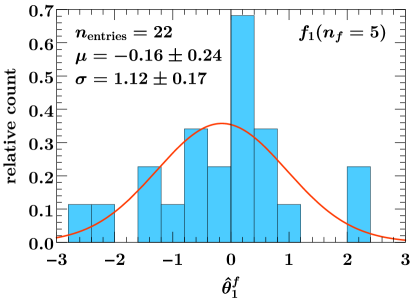
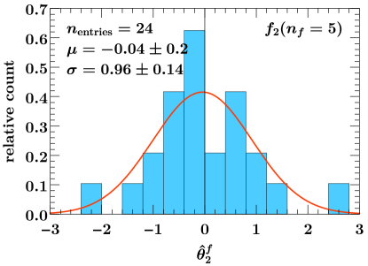
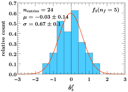
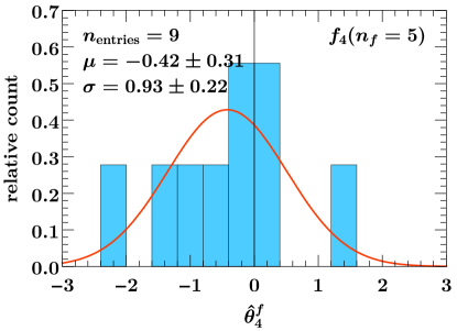
Figure -839: Distribution of true values of theory nuisance parameters for QCD matrix-element constants for $n_{f}=5$ at $n$-loop order for $n=1$ to $4$.

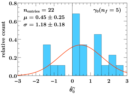
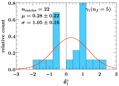
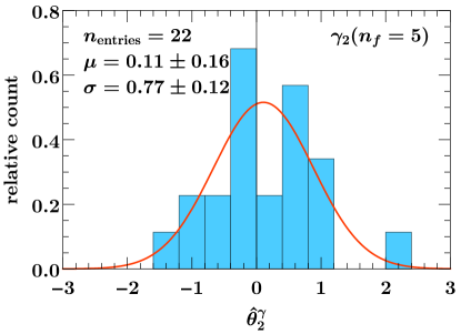
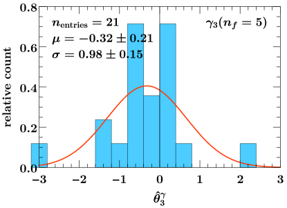
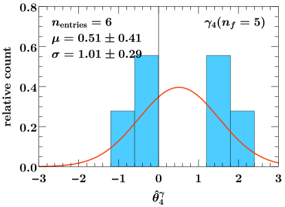
Figure -838: Distribution of true values of theory nuisance parameters for QCD anomalous dimensions for $n_{f}=5$ at $(n+1)$-loop order for $n+1=1$ to $5$.

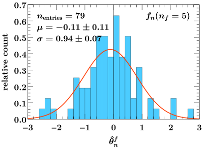
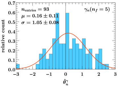
Figure -837: Distribution of true values of theory nuisance parameters for QCD matrix-element constants (left) and anomalous dimensions (right) for $n_{f}=5$ combining all available orders.

The sample distributions are shown for the matrix-element constants in figure -839 and for the anomalous dimensions in figure -838. The data is shown by the lightblue histograms. It is binned only for visualization purposes. For each sample, we perform an unbinned fit to a Gaussian distribution with mean $\mu$ and variance $\sigma^{2}$ as free parameters. The result is shown by the orange line and the fitted values for $\mu$ and $\sigma$ are quoted in each plot. The number of entries ($n_{\rm entries}$) for each sample is also given. The computed sample variance agrees with the fitted Gaussian variance to within a few percent in all cases except at the highest order with few entries where it differs by at most 10%.

We first observe that the standard deviation $\sigma$ for all samples is consistent with unity, which provides a clear validation of our natural-size estimate in section 5.2. (For the three-loop constants and anomalous dimensions the variance is somewhat smaller than one, which is not a concern.) The mean $\mu$ for the constants is very consistent with zero. The mean for the anomalous dimensions fluctuates a bit more, but is still largely consistent with zero. The shape of the sample distributions is generally well described by the Gaussian fit for the given number of fitted data points. The one-loop and two-loop anomalous dimensions show some noticable clusterings away from zero, which we can likely attribute to the fact that the their coefficients do not yet contain sufficient entropy.

Given that the samples for different $n$ all show similar distributions, with in particular the same mean and standard deviation within uncertainties, we can take a step further and assume that the populations for different $n$ can be described by a common distribution,

$$\hat{p}_{F_{n}}(x)\equiv\hat{p}_{F}(x)\qquad\forall n\,,$$ (5.12)

where $\hat{p}_{F}(x)$ is the distribution of all $\hat{\theta}_{n}$ in $F$ for any $n$. This allows us to combine the samples for different $n$ in each category. The resulting distributions of the combined samples for $F_{f}$ and $F_{\gamma}$ are shown in figure -837. Their approximately Gaussian shape is clearly evident. Most importantly, their fitted $\sigma=0.94\pm 0.07$ and $\sigma=1.05\pm 0.08$ are perfectly consistent with unity, and also agree with the computed sample variances. The means of the distributions $\mu=-0.11\pm 0.11$ and $\mu=0.16\pm 0.11$ show a small shift away from zero, but they are still consistent with zero. We could in principle account for this shift by adjusting our estimated central value. However, given that the effect is only marginal, we do not see a good reason for doing so in practice at this point.

In summary, we find very strong and convincing evidence for the robustness of our estimation procedure. Based on a large sample of known series coefficients, and with the identification in eq. (5.11), we find the distribution $p(\theta_{n})$ in eqs. (5.9) and (5.10) to have approximately zero mean and unit variance, confirming our original estimate of $u_{n}=0$ with $\Delta u_{n}=1$. We further find it to be well approximated by a Gaussian in agreement with our original assumption.

5.3.3 Further discussion

The fact that our estimation procedure yields distributions closely resembling Gaussians as in figure -837 speaks for itself. This can be contrasted with the very long-tailed distributions obtained from an analogous exercise using scale variations in ref. [7] or the typically very non-Gaussian distributions produced by the methods of refs. [2, 3, 4, 5].

It is also undeniable that the distributions are closer to a Gaussian than a flat box, in contrast to what one might have expected, as such a box-like distribution is sometimes advocated to be more appropriate than a Gaussian for perturbative theory uncertainties (albeit typically in the context of scale variations). We might also ask why to expect the distributions $\hat{p}_{F_{n}}(\hat{\theta}_{n})$ and $\hat{p}_{F}(\hat{\theta}_{n})$ to be sensible or useful in the first place. In fact, even though the $\hat{f}_{n}\in F_{n}$ all belong to some common category of perturbative series, we want this category to be as broad as possible to be as useful as possible. This means the distribution of $\hat{f}_{n}$, which is solely a property of the collection $F_{n}$ might very well be quite irregular and not very useful by itself. However, as we have stressed already, the distribution $\hat{p}_{F_{n}}(\hat{\theta}_{n})$ is a property of our estimation procedure for $F_{n}$. Its goal is precisely to strip the $\hat{f}_{n}$ of their individuality and reduce them to a generic bunch of numbers of a common more-or-less random origin, namely arising as a more-or-less random sum of Feynman diagrams. It is then perhaps not surprising after all that the resulting population of $\hat{\theta}_{n}$ can be well described by a Gaussian distribution. We might think of it as the central-limit theorem of Feynman diagrams.

It is also instructive to think about how we would notice if there was something going wrong in our estimation procedure. If we find a Gaussian with different mean or variance, then our estimation procedure itself is sound but our final choice of $u_{n}$ or $\Delta u_{n}$ is off, which we can easily adjust for if necessary. If the resulting distribution is irregular, e.g., with large tails or other undesired features, then this signals that our estimation procedure is suboptimal or missing some important aspect. A long tail would be indicative of underestimating the natural size for some coefficients in $F_{n}$. To illustrate this with a simple example, imagine we had not accounted for the overall $C_{r}$ color factor. As long as our collection $F_{n}$ contains only quark-like or only gluonic quantities, this would not be much of a problem, we would simply find an uncertainty of $C_{F}$ or $C_{A}$ instead of one. However, when $F_{n}$ contains both, we would end up with a superposition of two Gaussians of different variance. We could still work with this distribution, but it would be suboptimal because it would lead to overestimating the uncertainty for quark-like quantities and underestimating it for gluonic quantities.

This is also why it is prudent to consider separate collections $F_{n}$ for each $n$ at first, as this allows us to test and identify the appropriate $n$-dependent normalization. For example, without the $(n-1)!$ in $N_{n}^{f}$ in eq. (5.4) we would find distributions of correspondingly larger variance for $n\geq 3$, which is in fact how we became aware of this factor during the course of our investigations.

We conclude this subsection with two more comments. First, when applying our estimation procedure to a known $\theta_{n}$ we should not use our knowledge of its true value $\hat{\theta}_{n}$, but by including it in the sample of known $\hat{\theta}_{n}$ we do indirectly use it. However, this is acceptable since the impact of any one coefficient on the sample distribution is minor. Second, when applying our estimation procedure to a new and still unknown $\theta_{n}$, we still have to make a judgement whether or not it belongs to a particular category. There is a priori no guarantee for that. It might well be the case that there are genuinely different types of quantities than those considered so far that cannot be reduced to fit into an existing category but instead require defining and studying a new category.

5.4 Designing theory estimators

An interesting question to consider is whether it is possible to improve upon our estimator or design alternative estimators, which could be tested using the same procedure as above. We leave this for future investigation and only give some general remarks here. An improved estimator should on average yield a tighter estimate of the natural size but without underestimating it for some subset of series either. In other words, it should yield a reduced variance and ideally still produce a roughly Gaussian distribution.

For example, one could imagine devising an estimator based on the actual leading-color approximation of a series coefficient, i.e., using the large-$N_{c}$ expansion as a supplementary expansion following strategy 2 in section 4.3. This of course requires performing an actual calculation, but typically the calculation in the large-$N_{c}$ limit is easier to perform than the full calculation. Having a robust estimator based on this limit would allow one to robustly use such approximate results.

Another natural question that arises is whether one could utilize the information from the known lower orders $\hat{f}_{k<n}$ of a given quantity $f$ to improve the estimate for $f_{n}$. This effectively amounts to devising alternative parameterizations for $f_{n}$ involving the information of the known $\hat{f}_{k<n}$ in some way. In our intial attempts we found that this overall leads to less reliable estimates. For example, Padé approximations can work extremely well in some cases and utterly fail in others. The basic problem of relying on lower-order information is that this introduces the same generic pitfall also present for scale variations: It can lead to random significant underestimations when the lower-order coefficient(s) happen to be randomly smaller than their own natural size. This is in fact not unlikely to happen since as we have seen the mean of the distribution of true values is around 0. Examples of this are already present in tables 2 and 3, namely $\hat{f}_{1}$ of $c_{q\bar{q}S}$, $\hat{f}_{2}$ of $c_{gg}$, and notably $\hat{\gamma}_{3}$ of $\Gamma_{\mathrm{cusp}}^{q}$.

One might also consider applying the Bayesian inference models of refs. [2, 3, 4, 5] to estimate a given $\theta_{n}$ based on its known lower-order $\hat{\theta}_{k<n}$, as was mentioned already in ref. [4]. In this case, similar care has to be exercised to avoid the above pitfall. Another general option would be to utilize series transformations or series acceleration methods as in ref. [6]. In fact, taking the square root of a quantity can be considered a simple form of a series transformation.

From our experience so far, the most useful way to utilize the known lower-order information is as an important cross check of the estimation procedure rather than as a direct input to it. If a quantity consistently violates its estimated natural size at lower orders, it might indicate that we are not estimating its natural size correctly, which can have various reasons. We might be using the wrong normalization factor or a suboptimal reference scheme, or we might be associating it incorrectly with a given category. The latter can happen when not using the appropriate conventions, e.g. we should be parameterizing $\sqrt{f}$ or $f^{2}$ instead of $f$. It can also happen when we are using a suboptimal parameterization, for example when the scalar series has important internal structures (e.g. new color or partonic channels) which affect its natural size but which we have not explicitly parameterized.

More generally, the question is to what extent the higher-order coefficients are correlated with the lower-order ones and how to best exploit this correlation to our advantage. Such correlations could arise for example from cross terms of lower-order coefficients appearing as part of the higher-order coefficient (an obvious example is again using $f^{2}$ instead of $f$), or we believe the higher-order correction to be a genuinely multiplicative correction on top of the lower-order result (in which case we would parameterize their ratio). In general, such information is specific to a given quantity $f$. Therefore, all genuine lower-order information that we believe to be relevant should be accounted for explicitly by the specific parameterization of $f_{n}(\theta_{n})$ itself. An optimal parameterization would then be one for which the $\theta_{n}$ are uncorrelated for different $n$. In this limit, no more information can be gained from the lower-order $\hat{\theta}_{k<n}$ and the easiest and safest approach is to estimate the natural size of $\theta_{n}$ without further reference to $\hat{\theta}_{k<n}$. The boundary between parameterization and estimation is of course somewhat blurry, since as we have seen, the final step of parameterizing the remaining scalar coefficients in terms of scalar TNPs is in fact an important part of the estimation procedure itself.

6 Application to Transverse-Momentum Resummation

The $q_{T}$ spectrum of $Z$ and $W$ bosons produced in hadronic collisions, where $q_{T}\equiv p_{T}^{Z,W}$ is the transverse momentum of the produced vector boson, is a benchmark observable of the LHC precision physics program and has been measured to incredible precision by the ATLAS [57, 58, 59, 60], CMS [61, 62, 63], and LHCb collaborations [64, 65]. In this section, we discuss the application of our approach to precision predictions for the $q_{T}$ spectrum using resummed perturbation theory.

Correlations within the $p_{T}^{W}$ and $p_{T}^{\ell}$ spectra, and depending on the analysis strategy also between $p_{T}^{W}$ and $p_{T}^{Z}$, are critical for a precise measurement of the $W$-boson mass at hadron colliders [66, 67, 68, 69, 1]. As shown in ref. [14], the theory correlations in $p_{T}^{Z}$ are also critical if one wants to perform fits to the precisely measured small-$p_{T}^{Z}$ spectrum to extract nonperturbative parameters [70, 71]) or the strong coupling constant [72, 73].

In section 6.1 we give a brief account of the aspects of $q_{T}$ factorization and resummation that are relevant to our discussion. In section 6.2 we identify and discuss the necessary TNPs, and in section 6.3 we present numerical results that illustrate the power of the TNP approach to obtain predictions with proper theory correlations. Finally in section 6.4, we briefly discuss the treatment of subleading effects, which we neglect here for simplicity.

6.1 Aspects of $q_{T}$ resummation

We denote the four-momentum of the vector boson by $q^{\mu}$, its invariant mass and rapidity by $Q\equiv\sqrt{q^{2}}$ and $Y$, and its transverse momentum by $q_{T}=\lvert{\vec{q}}_{T}\rvert$. The quantity of our interest is the cross section fully differential in $Q$, $Y$, and $q_{T}$, which we write for brevity as $\mathrm{d}\sigma/\mathrm{d}^{4}q$.

We start by applying strategy 2 of section 4.3 and expand the cross section in a power series in $\varepsilon\equiv q_{T}^{2}/Q^{2}$,

$$\frac{\mathrm{d}\sigma}{\mathrm{d}^{4}q}=\frac{\mathrm{d}\sigma^{(0)}}{\mathrm{d}^{4}q}\Bigl{[}1+\mathcal{O}\Bigl{(}\frac{q_{T}^{2}}{Q^{2}}\Bigr{)}\Bigr{]}\,.$$ (6.1)

Compared to our discussion in section 4.3, where we expanded the series coefficient in $\varepsilon$, here it is much more useful to first perform the expansion in $\varepsilon$ and only later the perturbative expansion in $\alpha_{s}$. The reason is that we actually know the functional form in $q_{T}$ (and $Q$) of the leading-power term $\mathrm{d}\sigma^{(0)}$ to all orders in $\alpha_{s}$, allowing us to apply strategy 1 and obtain the exact correlations in $q_{T}$ and $Q$. Furthermore, we will also resum certain parts of the perturbative series to all orders in $\alpha_{s}$, although the precise way of doing so is not of immediate concern to us here, so we will not discuss it but refer the interested reader to refs. [38, 40].

The power expansion in eq. (6.1) converges very well, even better than the $q_{T}^{2}/Q^{2}$ scaling suggests, such that the power corrections remain below $\lesssim 5\%$ even up to moderately large $q_{T}\lesssim Q/3$ and even $Q/2$. As a result, the leading-power term $\mathrm{d}\sigma^{(0)}$ dominates and effectively determines the spectrum over this entire small-$q_{T}$ region, and thus also causes the dominant perturbative uncertainties. We can therefore focus our discussion on $\mathrm{d}\sigma^{(0)}$. In particular, it will serve us to demonstrate a nontrivial example application of the TNP approach. We will comment further on the treatment of the $\mathcal{O}(q_{T}^{2}/Q^{2})$ power corrections and other subleading effects in section 6.4.

The leading-power term $\mathrm{d}\sigma^{(0)}$ is the subject of the $q_{T}$ factorization and resummation program. We do not intend to provide a detailed review of $q_{T}$ resummation here. Rather, our focus is on the kinematic and process dependence, which we wish to break down and parameterize in terms of theory nuisance parameters. We use the SCET resummation framework of refs. [38, 40]. We closely follow the notation of those references and refer there for more details and further references. The leading-power cross section can be written as

$$\frac{\mathrm{d}\sigma^{(0)}}{\mathrm{d}^{4}q} =\frac{1}{2E_{\mathrm{cm}}^{2}}\,L_{VV^{\prime}}(q^{2})\,\sum_{a,b}H_{VV^{\prime}\,ab}(q^{2},\mu)$$ (6.2)

$$\quad\times\int\!\!\frac{\mathrm{d}^{2}{\vec{b}}_{T}}{(2\pi)^{2}}\,e^{\mathrm{i}{\vec{b}}_{T}\cdot{\vec{q}}_{T}}\,\tilde{B}_{a}(x_{a},b_{T},\mu,\nu/Q)\,\tilde{B}_{b}(x_{b},b_{T},\mu,\nu/Q)\tilde{S}(b_{T},\mu,\nu)\,.$$

Here, $VV^{\prime}=\{\gamma\gamma,\gamma Z,Z\gamma,ZZ,W^{+}W^{+},W^{-}W^{-}\}$ labels the produced vector boson including possible interferences. The leptonic tensor $L_{VV^{\prime}}(q^{2})$ contains the vector-boson propagator and decay and receives no QCD corrections, so its $q^{2}$ dependence is known. The hard function $H_{VV^{\prime}\,ab}(Q^{2},\mu)$ encodes the production of the vector boson in the underlying hard interaction $ab\to V$, with the sum over $a,b$ running over all relevant combinations of quark and antiquark flavors. The functional form of its $q^{2}$ and process dependence is known to all orders. The second line in eq. (6.2) contains all soft and collinear physics at the low scale $\mu\sim q_{T}$ encoded respectively in the soft function $\tilde{S}$ and beam function $\tilde{B}_{a,b}$. The $q_{T}$ dependence arises entirely from the second line, and its functional form is fully determined by the functional dependence on its Fourier-conjugate variable $b_{T}=\lvert{\vec{b}}_{T}\rvert$. The functional form of the $b_{T}$ dependence of the beam and soft functions is in turn known to all orders in $\alpha_{s}$. The beam function also depends on the flavor of the (anti)quark participating in the hard interaction and on $Q$. The functional form of these dependencies is also known to all orders. Finally, the variables $x_{a,b}=(Q/E_{\mathrm{cm}})e^{\pm Y}$ encode the dependence on the rapidity $Y$ and center-of-mass energy $E_{\mathrm{cm}}$. The functional form of the $x_{a,b}$ dependence of the beam function is not known to all orders but depends on their perturbative order.

The factorization in eq. (6.2) is very powerful for our purposes as it predicts the complete functional form in $q_{T}$ and also in $Q$ for given $x_{a,b}$. Furthermore, it fully parameterizes the exact dependence on the process and partonic channels. We are therefore able to apply strategy 1 and obtain exact correlations in all these dependencies. Although it does not predict the complete functional form in $x_{a,b}$ it still reduces it from a generic two-dimensional dependence to a product of common, universal one-dimensional beam functions.

For simplicity we have limited ourselves to the inclusive $q_{T}$ spectrum in eq. (6.2). Including the full kinematics of the vector-boson decay products is also possible. Importantly, at leading power doing so only increases the complexity of the leptonic tensor but does not induce any additional sources of QCD uncertainties [38]. We can therefore also capture the correlations in leptonic kinematic variables, most notably the lepton transverse momentum $p_{T}^{\ell}$, or between the $q_{T}$ spectrum and the $q_{T}$-dependent forward-backward asymmetry.

In principle, eq. (6.2) could be applied to each coefficient of the perturbative series of $\mathrm{d}\sigma^{(0)}$. However, at each order in $\alpha_{s}$, (double) logarithms of $q_{T}/Q$ appear, which render a fixed-order expansion of $\mathrm{d}\sigma^{(0)}$ unstable. Instead, eq. (6.2) also provides the basis for systematically resumming the unstable logarithmic contributions to all orders in $\alpha_{s}$, leading to precise and perturbatively stable predictions. We will not discuss how the resummation is carried out in practice but refer to refs. [38, 40] for details. The key point for us is that a given perturbative resummation order, NⁿLL, is uniquely defined by including all underlying scalar perturbative series discussed below to a specific order in $\alpha_{s}$. We then define our generalized counting including TNPs, N^n+kLL, to include the true values for all coefficients relevant for NⁿLL and in addition for each series the TNP parameterization of the next $k$ terms. In analogy to section 3.2, we also define the approximate Nⁿ⁺⁰LL implementation by absorbing the TNPs appearing at Nⁿ⁺¹LL as an additive correction to the respective highest coefficients appearing at NⁿLL.

6.2 TNPs for $q_{T}$ resummation

The perturbative ingredients required in eq. (6.2) are the hard, beam, and soft functions. Their functional dependence on the kinematic variables, except $x$, is fully predicted to all orders in $\alpha_{s}$ by their renormalization group equations, which we now discuss in turn. At the end we will be left with a set of (mostly) scalar perturbative series that fully determine the (fixed-order and/or resummed) perturbative series of $\mathrm{d}\sigma^{(0)}$. We will give a summary in section 6.2.4, so readers not interested in the detailed definnitions can directly skip there.

6.2.1 Hard function

The leptonic tensors for inclusive $Z\to\ell\ell$ and $W\to\ell\nu$ in eq. (6.2) are given by

$$L_{ZZ}(q^{2}) =\frac{2}{3}\frac{\alpha_{\mathrm{em}}}{q^{2}}\,(v_{\ell}^{2}+a_{\ell}^{2})\,\biggl{\lvert}\frac{q^{2}}{q^{2}-m_{Z}^{2}+\mathrm{i}\Gamma_{Z}m_{Z}}\biggr{\rvert}^{2}\,,$$

$$L_{W^{+}W^{+}}(q^{2}) =\frac{1}{6}\frac{\alpha_{\mathrm{em}}}{q^{2}}\,\frac{1}{\sin^{2}\theta_{w}}\,\biggl{\lvert}\frac{q^{2}}{q^{2}-m_{W}^{2}+\mathrm{i}\Gamma_{W}m_{Z}}\biggr{\rvert}^{2}\,.$$ (6.3)

Their $q^{2}$ dependence is known exactly in QCD. The corresponding hard functions have the form

$$H_{ZZ\,q\bar{q}^{\prime}}(q^{2},\mu) =\frac{8\pi\alpha_{\mathrm{em}}}{N_{c}}\delta_{qq^{\prime}}\biggl{\{}(v_{q}^{2}+a_{q}^{2})\lvert C_{q}(q^{2},\mu)\rvert^{2}$$

$$\quad+2\Re\sum_{f}\Bigl{[}v_{q}v_{f}C_{q}^{*}(q^{2},\mu)C_{vf}(q^{2},\mu)+a_{q}a_{f}C_{q}^{*}(q^{2},\mu)C_{af}(q^{2},\mu)\Bigr{]}+\dotsb\biggr{\}}\,,$$

$$H_{W^{+}W^{+}\,q\bar{q}^{\prime}}(q^{2},\mu) =\frac{2\pi\alpha_{\mathrm{em}}}{N_{c}}\frac{\lvert V_{qq^{\prime}}\rvert^{2}}{\sin^{2}\theta_{w}}\lvert C_{q}(q^{2},\mu)\rvert^{2}\,.$$ (6.4)

The expressions for the remaining $VV^{\prime}$ combinations can be found in appendix A of ref. [38]. The $v_{i}$ and $a_{i}$ are the usual axial and vector couplings of the $Z$ boson, $Q_{q}$ is the electromagnetic charge of quark $q$, and $V_{qq^{\prime}}$ are the CKM-matrix elements.

The $q^{2}$ dependence of the hard function is determined by that of the matching coefficients $C_{i}(q^{2},\mu)$, which correspond to the infriared-finite parts of the respective QCD form factors. Here, $C_{q}=1+\mathcal{O}(\alpha_{s}^{2})$ is the dominant vector nonsinglet coefficient corresponding to diagrams where the vector boson couples to the external quark line. The $C_{af}$ and $C_{vf}$ in eq. (6.2.1) are axial-singlet and vector-singlet coefficients corresponding to diagrams where the vector boson couples to a closed fermion loop, which only contribute to $Z$ production but not to $W$ production. They have separate perturbative series starting at $\mathcal{O}(\alpha_{s}^{2})$ and $\mathcal{O}(\alpha_{s}^{3})$, respectively, and have to be parametrized separately. In practice, their contributions are very small even at the order they contribute [40], so we can neglect them here for simplicity. In principle they would have to be included (starting at N³LL) to fully account for the correct (de)correlation between $W$ and $Z$ production. The ellipses in $H_{ZZ\,q\bar{q}^{\prime}}$ denote terms proportional to the square of $C_{af}$ and $C_{vf}$, which only contribute starting at $\mathcal{O}(\alpha_{s}^{4})$.

The functional form of the $q^{2}$ dependence of $C_{q}(q^{2},\mu)$ is known because by dimensional analysis it can only depend on the ratio $q^{2}/\mu^{2}$. The $q^{2}$ dependence is therefore fully predicted by the $\mu$ dependence, which in turn is governed by $C_{q}$’s renormalization group evolution (RGE) equation,

$$\mu\frac{\mathrm{d}}{\mathrm{d}\mu}\ln C_{q}(q^{2},\mu) =\Gamma_{\mathrm{cusp}}^{q}[\alpha_{s}(\mu)]\ln\frac{-q^{2}-\mathrm{i}0}{\mu^{2}}+2\gamma_{C}^{q}[\alpha_{s}(\mu)]\,.$$ (6.5)

The full $q^{2}$ and $\mu$ dependence of $C_{q}$ can be reconstructed by solving eq. (6.5) (either order by order in $\alpha_{s}$ or to all orders to obtain its resummed expression).

The cusp and noncusp anomalous dimensions $\Gamma_{\mathrm{cusp}}^{q}(\alpha_{s})$ and $\gamma_{C}^{q}(\alpha_{s})$ in eq. (6.5) are already scalar series. Following our conventions for anomalous dimensions in section 5.2, we parameterize

$$\Gamma(\alpha_{s})\equiv 2\Gamma_{\mathrm{cusp}}^{q}(\alpha_{s})\,,\qquad\gamma_{\mu}(\alpha_{s})\equiv 2\gamma_{C}^{q}(\alpha_{s})\,,$$ (6.6)

in terms of corresponding TNPs $\theta_{n}^{\Gamma}$ and $\theta_{n}^{\gamma_{\mu}}$.

The remaining nontrivial part of $C_{q}$ we need to parameterize is the $q^{2}$ and $\mu$-independent constant term, which is not predicted by eq. (6.5) and effectively acts as the boundary condition for solving the differential equation. We can formally define it as the matching coefficient evaluated at the canonical scale $\mu^{2}=-q^{2}$,

$$c_{q}(\alpha_{s})\equiv C_{q}(q^{2},\mu^{2}=-q^{2})\,.$$ (6.7)

By choosing the canonical scale proportional to $q^{2}$, the perturbative series for $c_{q}(\alpha_{s})$ becomes a scalar series with $q^{2}$ and $\mu$ independent coefficients. Here, $c_{q}(\alpha_{s}$ is equal to $c_{q\bar{q}V}(\alpha_{s})$ in section 5.2, so we parameterize it directly in terms of TNPs $\theta_{n}^{H}$, where the label is meant to remind us that they come from the hard function.

Note that the matching coefficient is defined in a certain renormalization scheme, for which we use the standard $\overline{\text{MS}}$ scheme here. Together with the canonical scale choice, which also determines the form of the logarithm in eq. (6.5), this defines the reference scheme for the anomalous dimensions and constant term and their TNPs.

6.2.2 Soft function

The TNP parameterization of the soft function $\tilde{S}(b_{T},\mu,\nu)$ proceeds analogously to that of the matching coefficient $C_{q}(q^{2},\mu)$ above. A new element is the soft function’s dependence on the additional rapidity renormalization scale $\nu$, which has dimension one. By dimensional analysis, the soft function can only depend on two ratios $b_{T}/\mu$ and $\mu/\nu$, so its full $b_{T}$ dependence is determined by its dependence on $\mu$ and $\nu$, which is now governed by a system of RGE equations,

$$\mu\frac{\mathrm{d}}{\mathrm{d}\mu}\ln\tilde{S}(b_{T},\mu,\nu) =4\Gamma_{\mathrm{cusp}}^{q}[\alpha_{s}(\mu)]\ln\frac{\mu}{\nu}+\tilde{\gamma}_{S}[\alpha_{s}(\mu)]\,,$$

$$\nu\frac{\mathrm{d}}{\mathrm{d}\nu}\ln\tilde{S}(b_{T},\mu,\nu) =\tilde{\gamma}_{\nu}(b_{T},\mu)\,,$$

$$\mu\frac{\mathrm{d}}{\mathrm{d}\mu}\tilde{\gamma}_{\nu}(b_{T},\mu) =-4\Gamma^{q}_{\mathrm{cusp}}[\alpha_{s}(\mu)]\,.$$ (6.8)

Here, the rapidity anomalous dimensions $\tilde{\gamma}_{\nu}(b_{T},\mu)$ has a more nontrivial dependence on $b_{T}$, which is in turn determined by its own $\mu$ dependence governed by its own $\mu$ RGE in the last line.

Solving eq. (6.2.2) now requires two independent boundary conditions, one for $\gamma_{\nu}(b_{T},\mu)$ and one for $\tilde{S}(b_{T},\mu,\nu)$ itself. The canonical scale in $b_{T}$ space is $\mu=b_{0}/b_{T}$ with $b_{0}=2e^{-\gamma_{E}}\approx 1.12291$, which corresponds to $\mu=q_{T}$ in momentum space. The soft function scales like a squared $2\to 0$ matrix element. Following our conventions in section 5.2, we therefore define the relevant scalar series as

$$\gamma_{\nu}(\alpha_{s})\equiv\frac{1}{2}\tilde{\gamma}_{\nu}(b_{T},\mu=b_{0}/b_{T})\,,$$

$$\tilde{s}(\alpha_{s})\equiv\sqrt{\tilde{S}(b_{T},\mu=b_{0}/b_{T},\nu=b_{0}/b_{T})}\,,$$ (6.9)

which we parameterize in terms of corresponding TNPs $\theta_{n}^{\gamma_{\nu}}$ and $\theta_{n}^{S}$. Note that the reference scheme for the TNPs here corresponds to our choices of using $b_{T}$ space and its canonical scale, $\overline{\text{MS}}$ renormalization, and rapidity renormalization [74] with the exponential regulator [75].

The other perturbative ingredients we need for the soft function are the cusp and noncusp anomalous dimensions in the first line of eq. (6.2.2). Following our conventions we would again parameterize $\Gamma(\alpha_{s})\equiv 2\Gamma_{\mathrm{cusp}}^{q}(\alpha_{s})$, consistent with eq. (6.6), and $\gamma_{S}(\alpha_{s})=\tilde{\gamma}_{S}(\alpha_{s})/2$. In practice, we do not need TNPs for $\gamma_{S}(\alpha_{s})$, for reasons we will explain in a moment.

6.2.3 Beam functions

The beam function $\tilde{B}_{i}(x,b_{T},\mu,\nu/Q)$ only depends on the combination $\nu/Q$, as indicated by its argument, and thus by dimensional analysis only on $b_{T}/\mu$. Its $b_{T}$ and explicit $Q$ dependence is thus governed by its RGE system, which is closely analogous to that of the soft function in eq. (6.2.2),

$$\mu\frac{\mathrm{d}}{\mathrm{d}\mu}\ln\tilde{B}_{q}(x,b_{T},\mu,\nu/Q) =2\Gamma_{\mathrm{cusp}}^{q}[\alpha_{s}(\mu)]\ln\frac{\nu}{Q}+\tilde{\gamma}_{B}[\alpha_{s}(\mu)]\,,$$

$$\nu\frac{\mathrm{d}}{\mathrm{d}\nu}\ln\tilde{B}_{q}(x,b_{T},\mu,\nu/\omega) =-\frac{1}{2}\tilde{\gamma}_{\nu}(b_{T},\mu)\,,$$

$$\mu\frac{\mathrm{d}}{\mathrm{d}\mu}\tilde{\gamma}_{\nu}(b_{T},\mu) =-4\Gamma^{q}_{\mathrm{cusp}}[\alpha_{s}(\mu)]\,.$$ (6.10)

We need again the cusp and rapidity anomalous dimensions, which are the same as before in eq. (6.2.2), the noncusp beam anomalous dimension $\gamma_{B}(\alpha_{s})\equiv\tilde{\gamma}_{B}(\alpha_{s})$, and the beam function boundary condition.

We do not need TNPs for the beam and soft noncusp anomalous dimensions for the following reason. When using the beam and soft function’s RGEs to reconstruct their full fixed-order expressions, we only need the known anomalous dimension coefficients (for our considered resummation orders). Their TNPs would only enter in the evolution itself. However, since the beam and soft functions start their evolution at the same canonical scale $\mu=b_{0}/b_{T}$, only their total $\mu$ anomalous dimension actually enters in the resummation, which by consistency is equal to minus that of the hard function. We therefore only need the single noncusp $\mu$ anomalous dimension in eq. (6.6).

Importantly, the RGEs do not depend on $x$, which implies that the additional $x$ dependence factorizes from the $b_{T}$ and $Q$ dependencies and only enters via the beam boundary condition, which is now defined at the canonical scales $\mu=b_{0}/b_{T}$ and $\nu=Q$,

$$\tilde{b}_{i}(x,\alpha_{s})\equiv\tilde{B}_{i}(x,b_{T},\mu=b_{0}/b_{T},\nu/Q=1)\,.$$ (6.11)

The additional complication for the beam function arises because its $x$ dependence is not predicted by its RGE, so the beam boundary condition is a general one-dimensional function of $x$. To further break down this dependence, we calculate its series coefficients $\tilde{b}_{i,n}(x)$ in terms of collinear PDFs $f_{j}(x)$,

$$\tilde{b}_{i,n}(x) =\sum_{j}\int\!\frac{\mathrm{d}z}{z}\,\tilde{I}_{ij,n}(z)\,f_{j}\Bigl{(}\frac{x}{z}\Bigr{)}\,,$$ (6.12)

where $\tilde{I}_{ij,n}(z)$ are perturbatively calculable matching kernels. The $x$ dependence of the beam function is thus determined via the Mellin convolution of the $x$ dependence of the PDFs and the $z$ dependence of the matching kernels. Since the $x$ dependence of the PDFs tends to be quite strong, the mix of contributing PDFs determines the overall size of $\tilde{b}_{i,n}(x)$ as well as playing an important role in determining its shape in $x$. The $I_{ij,n}(z)$ are perturbative coefficients, so we can in principle estimate their natural size as in section 5.2. (In fact, their moments in $x$ enter into our sample of matrix-element constants). In contrast, it would be quite difficult to estimate the natural size of $\tilde{b}_{i,n}(x)$ directly. Eq. (6.12) is thus an example where parameterizing a dependence (here the channel dependence) is beneficial or even necessary for obtaining a natural-size estimate.

Following our discussion in section 4, if we do not require precise correlations in $x$, one option would be to only parameterize the integral of $I_{ij,n}(z)$, with e.g. a trivial $z$ dependence $\sim\delta(1-z)$. If we do require proper correlations in $x$, i.e. in $Y$ and/or $E_{\mathrm{cm}}$, we need to properly parameterize the $z$ dependence. At the orders we are working their true expressions are actually known [76, 77]. Therefore, as a starting point we parameterize them using their known functional form in $z$ multiplied by an overall scalar coefficient

$$\tilde{I}_{ij,n}(z,\theta_{n}^{B_{ij}})=\frac{3}{2}\,\theta_{n}^{B_{ij}}\,\hat{\tilde{I}}_{ij,n}(z)\,,$$ (6.13)

where we include a factor of $3/2$ to be conservative and account for the fact that their true values are typically somewhat below their natural size. Another option would be to explicitly normalize the $\hat{\tilde{I}}_{ij,n}(z)$ in some way.

With the TNP parameterization in eq. (6.13), we effectively treat the shape as exactly known, while the overall normalization is unknown. We prefer this option to using $\delta(1-z)$, because it means we have the exact correlations for the overall normalization uncertainty we do consider. Of course, at the highest known order we cannot do that, and strictly speaking at lower orders we should not be allowed to use the known shape but include some shape uncertainties. In the future, the $z$ dependence of the matching kernels can be explicitly parameterized using strategy 2 by expanding them in $\varepsilon=1-z$, since their $z\to 1$ limit is actually well understood [43].

The dominant partonic channels are $ij=\{qqV,qg\}$, which start at $\mathcal{O}(1)$ and $\mathcal{O}(\alpha_{s})$. At higher orders, further singlet channels $ij=\{q\bar{q}V,qqS$, $qq\Delta S\}$ appear, whose precise definition is given in ref. [43]. Since they only give small corrections even at the order they appear, for our numerical results in section 6.3 we only consider two TNPs for the beam boundary condition, namely a single effective $\theta_{n}^{B_{qq}}$,

$$\theta_{n}^{B_{qq}}\equiv\theta_{n}^{B_{qqV}}\equiv\theta_{n}^{B_{q\bar{q}V}}\equiv\theta_{n}^{B_{qqS}}\equiv\theta_{n}^{B_{qq\Delta S}}\,,$$ (6.14)

which collectively varies all $qq$ channels together with $\theta_{n}^{B_{qg}}$ for the $qg$ channel.

In principle, we also have to include the QCD splitting functions, which govern the evolution of the PDFs, in our counting. In the resummed cross section, the PDFs enter through the beam functions where they are evaluated at the scale of the beam function, which means their evolution contributes to the $q_{T}$ resummation by resumming single logarithms of $b_{T}$. That is, they count as a noncusp anomalous dimension. Constructing TNP paramterizations for the splitting functions can be done similarly to the beam function matching kernels by considering their $z\to 1$ and also $z\to 0$ limits. In fact, in this way TNPs for the four-loop splitting functions have already been considered in ref. [11] including constraints from their known moments. Since varying the splitting functions is rather involved technically, as it requires re-evolving the PDFs, we refrain from doing so here, and leave this for future work. Instead, if needed, this source of uncertainty can be probed for now by conventional $\mu_{F}$ variations.

6.2.4 Summary of TNPs

To summarize, we have a minimum of seven TNPs, corresponding to seven independent perturbative ingredients and thus sources of uncertainty: Three anomalous dimensions and four boundary conditions, which belong to the category of matrix-element constants,

$$\theta_{n}^{\gamma}:\gamma\in\{\Gamma,\gamma_{\mu},\gamma_{\nu}\}\,,\qquad\theta_{n}^{f}:f\in\{H,S,B_{qq},B_{qg}\}\,.$$ (6.15)

There is actually one piece of perturbative information that we have silently taken for granted so far: The solution of the RGEs also requires the QCD $\beta$ function, because it governs the $\mu$ dependence of $\alpha_{s}(\mu)$, and its TNP would in principle enter in the resummation at the same loop order as the TNP of the cusp anomalous dimension. In practice however, while the overall $\mu$ evolution of $\alpha_{s}(\mu)$ is important, the higher-order corrections to it tend to be numerically very small. We therefore continue to treat the $\beta$ function as known to avoid adding significant but unnecessary complexity.

In addition to the above 7 TNPs (or 6 if we are willing to count the beam function as a single one), we have 3 (or 4) more once we account for the full set of partonic channels of the beam function (still without accounting for its functional dependence). In addition, we have $2$ more once we account for singlet contributions to the hard function, $1$ more if we also count the $\beta$ function, and several more once we account for the splitting functions.

Let us contrast this with a scale-variation based approach to estimate perturbative uncertainties. Even the most sophisticated currently available scale-variation-based setup [40] involves 5 scales ($\mu_{H}$, $\mu_{B}$, $\mu_{S}$, $\nu_{B}$, $\nu_{S}$) that are being varied, which thus cannot begin to capture even the minimal space of theory uncertainties and correlations. And in most other approaches to $q_{T}$ resummation even fewer scales are considered.

6.3 Numerical results

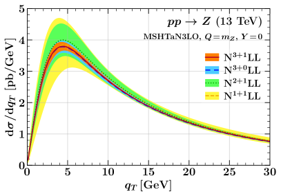
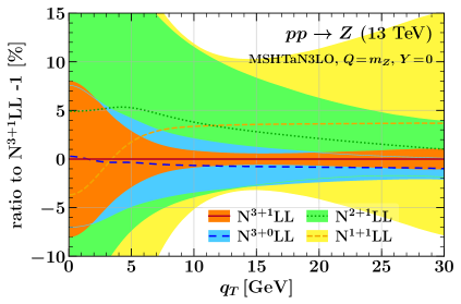
Figure -836: Leading-power $q_{T}\equiv p_{T}^{Z}$ spectrum for inclusive $pp\to Z$ production at the 13 TeV LHC at N²⁺¹LL (green), N³⁺⁰LL (blue), and N³⁺¹LL (orange). The results are shown for the absolute spectrum on the left and as the relative difference to the N³⁺¹LL central value on the right. The bands show the total theory uncertainty at 95% theory CL.

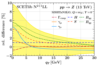
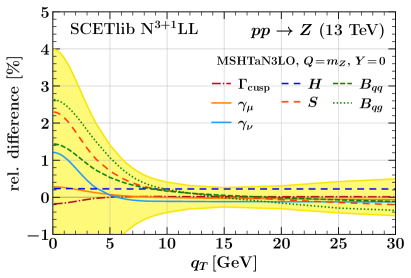
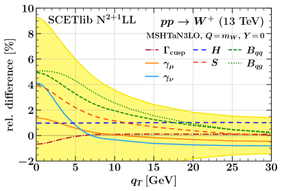
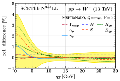
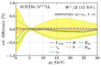
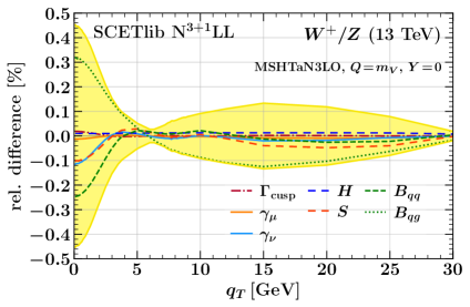
Figure -835: Breakdown of the relative uncertainties in the leading-power $q_{T}\equiv p_{T}^{Z,W}$ spectrum at the 13 TeV LHC at N²⁺¹LL (left panels) and N³⁺¹LL (right panels) for $pp\to Z$ (top row), $pp\to W^{+}$ (middle row), and their ratio (bottom row). The different lines show the impact of varying the corresponding theory nuisance parameter by $+1$ or $-1$, corresponding to 68% theory CL. The yellow band shows their sum in quadrature. See the text for more details.

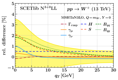
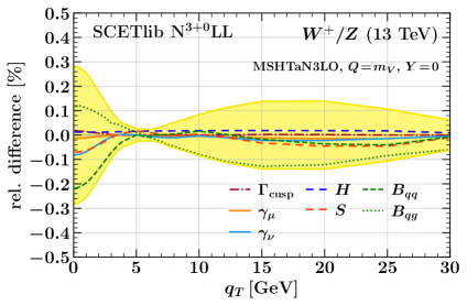
Figure -834: Same as figure -835 but for the approximate implementation at N³⁺⁰LL.

For our numerical results for the leading-power $q_{T}$ spectrum, we consider inclusive $pp\to V$ production with $V=Z,W^{\pm}$ at the 13 TeV LHC at fixed invariant mass $Q\equiv\sqrt{q^{2}}=m_{V}$ and rapidity $Y=0$ of the vector boson, unless noted otherwise. We use the MSHT20an3lo [11] PDF set with $\alpha_{s}(m_{Z})=0.118$. All results are obtained with SCETlib [78] based on its implementation of $q_{T}$ resummation up to N⁴LL [43, 38, 39, 40], which we have extended to support the required theory nuisance parameter variations. Since we only consider the leading-power spectrum without matching to the full fixed-order result at large $q_{T}$, we restrict ourselves to $q_{T}\leq 30\,\mathrm{GeV}$, where the neglected $\mathcal{O}(q_{T}^{2}/Q^{2})$ and higher power corrections amount to at most a few-percent correction and the uncertainties associated with the matching procedure are also not yet relevant [40].

In figure -836, we start by presenting the $Z$ $q_{T}$ spectrum at different subsequent orders up to N³⁺¹LL. The uncertainty bands show the total theory uncertainty at 95% theory CL from varying all TNPs by $\Delta u_{n}=\pm 2$. Note that the N³⁺⁰LL result is an intermediate order, which is included for illustration and future reference.

In figure -835 we show the breakdown of the theory uncertainty by individual TNPs. The impacts on the spectrum from varying the TNPs up or down are roughly symmetric, so for clarity we always only show the $\Delta u_{n}=+1$ variation for the anomalous dimensions, hard function, and soft function, and the $\Delta u_{n}=-1$ variation for the beam function. Since each TNP corresponds to an independent source of uncertainty, which furthermore can be considered Gaussian distributed (see section 5), the correct way to combine them into a total uncertainty is to add them in quadrature. This is shown by the light yellow band, corresponding to the total uncertainty at 68% theory CL. In the top and middle rows we show the results for $Z$ and $W^{+}$ and in the bottom row their ratio.

Concerning the correlations in the shape of the $q_{T}$ spectrum, each of the TNP variations shown by the different lines in figure -835 reflects a 100% correlated uncertainty component across the $q_{T}$ spectrum. We observe that the different components have quite different shapes and include cases where the correlation is always positive as well as cases switching sign from correlated to anticorrelated at different points in $q_{T}$. Hence, as anticipated, it is not possible to correctly model the correlations in the $q_{T}$ spectrum by a 100% (anti)correlated hypothesis.

Let us briefly compare this to a scale-variation based approach. By scanning over different scale variations in order to account for the shape uncertainties, one is precisely scanning over various (more-or-less arbitrary) 100% (anti)correlated hypotheses. We remind the reader (see section 2.1.2) that when correlations matter, incorrect correlation assumptions can have dramatic consequences on the resulting uncertainties. In ref. [14], we will show explicitly that accounting for the proper correlations in $q_{T}$ is indeed absolutely critical if one wants to exploit precision measurements of the $q_{T}$ spectrum, particularly its extremely precisely measured shape, for interpretation purposes such as extracting nonperturbative parameters or the strong coupling constant. All current attempts at doing so, including the recent analysis in ref. [73], are based on scale variations and are thus subject to uncontrolled correlation assumptions in the underlying perturbative predictions. Hence, the quoted perturbative theory uncertainties in the extracted parameters of interest must be interpreted with extreme caution.

As expected, the uncertainties are very similar for the closely related $Z$ and $W$ processes, whose main differences are the different partonic channel combinations and the small difference in their masses. Since the TNPs for both processes are the same, each of the individual impacts are 100% correlated between the processes, and as a result cancel in the ratio to very large extent, roughly by a factor of 10. We stress that whilst a large degree of cancellation is expected and has been encountered many times before, we can now correctly quantify it for the first time, and in particular also its dependence on $q_{T}$.

In figure -834 we show the same results using the approximate implementation of the theory nuisance parameters at N³⁺⁰LL. This is the setup utilized for the resummed component of the $q_{T}$ spectrum in the analysis of ref. [1], where it is also further matched to the fixed-order NLO₁ result for the $V$+1-parton process. At N³⁺⁰LL, formally the same $\theta_{n}$ enter as at N³⁺¹LL but their impacts are only approximately correct. Namely, their shape is approximated by the corresponding one at N²⁺¹LL, while their overall impact is similar to that at N³⁺¹LL. Whilst the precise shapes of the components differ between N³⁺¹LL and N³⁺⁰LL their overall qualitative behaviour is similar. The total uncertainties at N³⁺⁰LL are similar to but somewhat larger than at full N³⁺¹LL. Notably, the uncertainties on the $W/Z$ ratio, which strongly depend on the detailed correlations, are very similar to those at N³⁺¹LL. Therefore, we can conclude that the N³⁺⁰LL result provides a clear improvement over N²⁺¹LL and a reasonable approximation to the more correct N³⁺¹LL result. Although the N³⁺¹LL result should be preferred, the approximate N³⁺⁰LL result can serve as a viable compromise if the former cannot be utilized for some reason. One such reason could be the availability of the required fixed-order matching at large $q_{T}$. Since N³⁺⁰LL implements the N³LL structure it can be consistently matched to NLO₁, whereas N³⁺¹LL implements the full N⁴LL structure and therefore requires matching to NNLO₁.

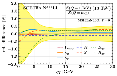
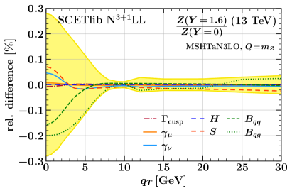
Figure -833: Relative uncertainties in the leading-power $q_{T}\equiv p_{T}^{Z}$ spectrum at the 13 TeV LHC at N³⁺¹LL for the ratio of $pp\to Z$ at $Q=1\,\mathrm{TeV}$ vs. $Q=m_{Z}$ (left) and $Y=1.6$ vs. $Y=0$ (right). The meaning of the curves is the same as in figure -835.

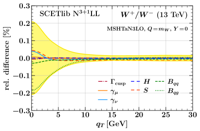
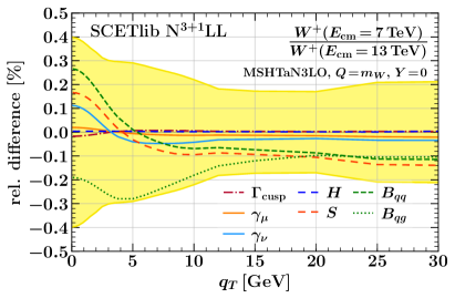
Figure -832: Relative uncertainties in the leading-power $q_{T}\equiv p_{T}^{W}$ spectrum at N³⁺¹LL for the ratio of $pp\to W^{+}$ vs. $pp\to W^{-}$ at the 13 TeV LHC (left) and $pp\to W^{+}$ at the 7 TeV LHC vs. 13 TeV LHC (right). The meaning of the curves is the same as in figure -835.

In figure -833 we show the ratios of the $q_{T}$ spectra for $Z$ production at $Q=1\,\mathrm{TeV}$ vs. $Q=m_{Z}$ and $Y=1.6$ vs. $Y=0$. Figure -832 shows the ratios of the $q_{T}$ spectra for $W^{+}$ vs. $W^{-}$ and for $W^{+}$ at 13 TeV vs. 7 TeV. The cancellation of uncertainties is expectedly most pronounced for $W^{+}/W^{-}$. It is weakest but still present for the case of $Q=1\,\mathrm{TeV}$ vs. $Q=m_{Z}$. This is also not unexpected, since the spectrum mostly depends on $q_{T}/Q$, so for different $Q$ the $q_{T}$ spectra are shifted against each other.

We stress that the primary purpose of the various ratios we show is to easily visualize the effect of correlations and the resulting degree of cancellations. When correctly accounting for the theory correlations there is no difference as far as theory uncertainties are concerned in using the ratio or the quantities separately. In a real analysis, one would typically not use ratios but simply perform a combined analysis of all relevant processes, which constrains the TNPs among all of them accounting for all correlations and resulting cancellations. In the limit where one particular process is much more precisely measured than the others, one can think of it as effectively acting as a control process to obtain improved predictions for the others.

An important observation is that the dominant uncertainties that remain in the ratios and tend to cancel the least are those due to the beam functions, in particular for $W/Z$ but also in many cases for the other ratios in figures -833 and -832. This is because the main difference between the processes, which is due to the different combinations of flavor channels, precisely enters via a different relative mix of different beam functions. This motivates a more detailed study of the beam function TNPs.

To conclude this section, we stress again that here we only consider the leading-power contributions. This is warranted as these are by far the dominant contributions to the spectrum at small $q_{T}$, so the precise correlation and resulting cancellation of their uncertainties is a critical ingredient to any interpretation of precision measurements of the $q_{T}$ spectrum, which we are able to properly take into account for the first time. The uncertainties in the ratios illustrate the level of precision that can now be reached via the cancellation of the dominant uncertainties in a combined analysis. At the resulting sub-percent level of precision, many other previously subleading effects can become equally or more important and must be accounted for to maintain this level of precision, motivating future work on them. We briefly comment on these in the next subsection.

6.4 Subleading effects

The application of our approach to the leading-power resummed contribution represents a crucial milestone toward a more complete and comprehensive understanding of the $q_{T}$ spectrum. A complete treatment also requires accounting for several other subdominant effects. These are in particular:

• The neglected subleading power corrections in eq. (6.1) starting at $\mathcal{O}(q_{T}^{2}/Q^{2})$.

• Effects due to finite quark masses of $\mathcal{O}(m_{q}^{2}/q_{T}^{2})$.

• QED and electroweak effects.

• Nonperturbative corrections of $\mathcal{O}(\Lambda_{\mathrm{QCD}}^{2}/q_{T}^{2})$.

The nonperturbative corrections already have a parametric nature. In the future, our approach can also be applied systematically to the first three effects following the methodology developed in the previous sections. In the absence of their complete TNP-based treatment, they can still be included from existing results based on conventional methods. In other words, a TNP treatment of even just the leading-power resummed component is already extremely valuable, simply because it contributes by far the dominant uncertainties.

7 Conclusions

The theory nuisance parameter approach developed in this paper holds enormous potential to make perturbative predictions more robust and also more precise:

• It allows for the first time to correctly account for theory correlations, which are important whenever one simultaneously interprets multiple measurements (including different bins in a spectrum).

• The theory uncertainties and correlations are straightforward to propagate, like any other nuisance parameters, into fits, Monte-Carlo generators, multivariate analyses, neural networks, etc.

• In fits to experimental measurements, it is possible and consistent to profile the theory nuisance parameters and thereby constrain them, effectively reducing the theory uncertainties by the measurements, which is not possible with existing methods.

• New structures (e.g. partonic channels or additional logarithmic powers) appearing at higher order are explicitly anticipated and accounted for by the theory uncertainties.

• All new, even partial, higher-order information can have immediate phenomenological impact in reducing theory uncertainties, even if the complete next order is not yet available.

• The theory uncertainties have a well-defined and meaningful statistical interpretation.

When applied to color-singlet transverse-momentum ($p_{T}$) resummation, the theory nuisance parameters allow one to correctly and fully account for the theory correlations in the shape of the small-$p_{T}$ spectrum, between different $Q$ values, partonic channels, hard processes (e.g. $W$ and $Z$ production), collider energies, and different resummation-sensitive variables (e.g. $p_{T}^{V}$, $p_{T}^{\ell}$ near the Jacobian peak, or $\phi^{*}$). In this context, our approach opens the door to reaching sub-percent level theoretical precision, which will be able to match the incredible precision already achieved by experimental measurements. To fully reach this level of theoretical precision, a variety of subleading effects must still be accounted for. We thus hope that our results also provide strong motivation for future work in this direction. For expedience, they can at first be included using conventional methods, which does not invalidate the TNP-based treatment of the dominant uncertainties. More importantly, our approach is also not limited to the dominant resummed contribution. It can be systematically and incrementally applied also to subleading effects as they become relevant at any given level of theory precision.

More generally, it will obviously be impossible to equip existing predictions with TNP-based uncertainties all at once. We should stress that this is also not required by the TNP approach. To the contrary, a more practical, incremental adoption, focusing on the dominant sources of uncertainties first is exactly in the spirit of our approach, namely to parameterize and include the sources of uncertainties in the theory predictions in order of their relevance.

References

- [1] CMS collaboration, Measurement of the W boson mass in proton-proton collisions at sqrts = 13 TeV, 2024, CMS-PAS-SMP-23-002.
- [2] M. Cacciari and N. Houdeau, Meaningful characterisation of perturbative theoretical uncertainties, JHEP 09 (2011) 039 [1105.5152].
- [3] E. Bagnaschi, M. Cacciari, A. Guffanti and L. Jenniches, An extensive survey of the estimation of uncertainties from missing higher orders in perturbative calculations, JHEP 02 (2015) 133 [1409.5036].
- [4] M. Bonvini, Probabilistic definition of the perturbative theoretical uncertainty from missing higher orders, Eur. Phys. J. C 80 (2020) 989 [2006.16293].
- [5] C. Duhr, A. Huss, A. Mazeliauskas and R. Szafron, An analysis of Bayesian estimates for missing higher orders in perturbative calculations, JHEP 09 (2021) 122 [2106.04585].
- [6] A. David and G. Passarino, How well can we guess theoretical uncertainties?, Phys. Lett. B 726 (2013) 266 [1307.1843].
- [7] A. Ghosh, B. Nachman, T. Plehn, L. Shire, T. M. P. Tait and D. Whiteson, Statistical patterns of theory uncertainties, SciPost Phys. Core 6 (2023) 045 [2210.15167].
- [8] G. Cowan, K. Cranmer, E. Gross and O. Vitells, Asymptotic formulae for likelihood-based tests of new physics, Eur. Phys. J. C 71 (2011) 1554 [1007.1727].
- [9] R. D. Cousins and L. Wasserman, PHYSTAT Informal Review: Marginalizing versus Profiling of Nuisance Parameters, 2404.17180.
- [10] F. J. Tackmann, Theory Uncertainties from Nuisance Parameters, March 2019, Talk at SCET 2019 workshop.
- [11] J. McGowan, T. Cridge, L. A. Harland-Lang and R. S. Thorne, Approximate N3LO parton distribution functions with theoretical uncertainties: MSHT20aN3LO PDFs, Eur. Phys. J. C 83 (2023) 185 [2207.04739].
- [12] B. Dehnadi, I. Novikov and F. J. Tackmann, The photon energy spectrum in at N3LL′, JHEP 07 (2023) 214 [2211.07663].
- [13] P. Cal, M. A. Lim, D. J. Scott, F. J. Tackmann and W. J. Waalewijn, Jet veto resummation for STXS 1-jet bins at aNNLL′+NNLO, 2408.13301.
- [14] T. Cridge, G. Marinelli and F. J. Tackmann, Theory uncertainties in the extraction of from Drell-Yan at small transverse momentum, 2024, (in preparation).
- [15] S. Moch, J. A. M. Vermaseren and A. Vogt, Higher-order corrections in threshold resummation, Nucl. Phys. B 726 (2005) 317 [hep-ph/0506288].
- [16] T. Becher and M. D. Schwartz, A precise determination of from LEP thrust data using effective field theory, JHEP 07 (2008) 034 [0803.0342].
- [17] R. Abbate, M. Fickinger, A. H. Hoang, V. Mateu and I. W. Stewart, Thrust at N3LL with Power Corrections and a Precision Global Fit for , Phys. Rev. D 83 (2011) 074021 [1006.3080].
- [18] T. Becher, M. Neubert and L. Rothen, Factorization and +NNLO predictions for the Higgs cross section with a jet veto, JHEP 10 (2013) 125 [1307.0025].
- [19] M. Bonvini and S. Marzani, Resummed Higgs cross section at N3LL, JHEP 09 (2014) 007 [1405.3654].
- [20] A. H. Hoang, D. W. Kolodrubetz, V. Mateu and I. W. Stewart, -parameter distribution at N3LL’ including power corrections, Phys. Rev. D 91 (2015) 094017 [1411.6633].
- [21] P. J. Mohr, B. N. Taylor and D. B. Newell, CODATA Recommended Values of the Fundamental Physical Constants: 2010, Rev. Mod. Phys. 84 (2012) 1527 [1203.5425].
- [22] S. Sturm, F. Köhler, J. Zatorski, A. Wagner, Z. Harman, G. Werth et al., High-precision measurement of the atomic mass of the electron, Nature 506 (2014) 467 [1406.5590].
- [23] L. Berthier and M. Trott, Consistent constraints on the Standard Model Effective Field Theory, JHEP 02 (2016) 069 [1508.05060].
- [24] S. Alte, M. König and W. Shepherd, Consistent Searches for SMEFT Effects in Non-Resonant Dijet Events, JHEP 01 (2018) 094 [1711.07484].
- [25] M. Trott, Methodology for theory uncertainties in the standard model effective field theory, Phys. Rev. D 104 (2021) 095023 [2106.13794].
- [26] A. Ghosh and B. Nachman, A cautionary tale of decorrelating theory uncertainties, Eur. Phys. J. C 82 (2022) 46 [2109.08159].
- [27] I. W. Stewart and F. J. Tackmann, Theory Uncertainties for Higgs and Other Searches Using Jet Bins, Phys. Rev. D 85 (2012) 034011 [1107.2117].
- [28] A. Banfi, G. P. Salam and G. Zanderighi, NLL+NNLO predictions for jet-veto efficiencies in Higgs-boson and Drell-Yan production, JHEP 06 (2012) 159 [1203.5773].
- [29] S. Gangal and F. J. Tackmann, Next-to-leading-order uncertainties in Higgs+2 jets from gluon fusion, Phys. Rev. D 87 (2013) 093008 [1302.5437].
- [30] LHC Higgs Cross Section Working Group collaboration, D. de Florian et al., Handbook of LHC Higgs Cross Sections: 4. Deciphering the Nature of the Higgs Sector, 1610.07922.
- [31] Les Houches 2017: Physics at TeV Colliders Standard Model Working Group Report, 3, 2018.
- [32] J. M. Lindert et al., Precise predictions for jets dark matter backgrounds, Eur. Phys. J. C 77 (2017) 829 [1705.04664].
- [33] L. A. Harland-Lang and R. S. Thorne, On the Consistent Use of Scale Variations in PDF Fits and Predictions, Eur. Phys. J. C 79 (2019) 225 [1811.08434].
- [34] NNPDF collaboration, R. Abdul Khalek et al., Parton Distributions with Theory Uncertainties: General Formalism and First Phenomenological Studies, Eur. Phys. J. C 79 (2019) 931 [1906.10698].
- [35] C. F. Berger, C. Marcantonini, I. W. Stewart, F. J. Tackmann and W. J. Waalewijn, Higgs Production with a Central Jet Veto at NNLL+NNLO, JHEP 04 (2011) 092 [1012.4480].
- [36] I. W. Stewart, F. J. Tackmann, J. R. Walsh and S. Zuberi, Jet resummation in Higgs production at NNLLNNLO, Phys. Rev. D89 (2014) 054001 [1307.1808].
- [37] W. Bizon, A. Gehrmann-De Ridder, T. Gehrmann, N. Glover, A. Huss, P. F. Monni et al., The transverse momentum spectrum of weak gauge bosons at N3LL+NNLO, Eur. Phys. J. C 79 (2019) 868 [1905.05171].
- [38] M. A. Ebert, J. K. L. Michel, I. W. Stewart and F. J. Tackmann, Drell-Yan resummation of fiducial power corrections at N3LL, JHEP 04 (2021) 102 [2006.11382].
- [39] G. Billis, B. Dehnadi, M. A. Ebert, J. K. L. Michel and F. J. Tackmann, Higgs pT Spectrum and Total Cross Section with Fiducial Cuts at Third Resummed and Fixed Order in QCD, Phys. Rev. Lett. 127 (2021) 072001 [2102.08039].
- [40] G. Billis, J. K. L. Michel and F. J. Tackmann, Drell-Yan Transverse-Momentum Spectra at N3LL′ and Approximate N4LL with SCETlib, 2411.16004.
- [41] L. N. Trefethen, Approximation Theory and Approximation Practice. Society for Industrial and Applied Mathematics, 2012.
- [42] Z. Ligeti, I. W. Stewart and F. J. Tackmann, Treating the b quark distribution function with reliable uncertainties, Phys. Rev. D 78 (2008) 114014 [0807.1926].
- [43] G. Billis, M. A. Ebert, J. K. L. Michel and F. J. Tackmann, A toolbox for and 0-jettiness subtractions at N3LO, Eur. Phys. J. Plus 136 (2021) 214 [1909.00811].
- [44] R. N. Lee, A. von Manteuffel, R. M. Schabinger, A. V. Smirnov, V. A. Smirnov and M. Steinhauser, Quark and Gluon Form Factors in Four-Loop QCD, Phys. Rev. Lett. 128 (2022) 212002 [2202.04660].
- [45] A. Chakraborty, T. Huber, R. N. Lee, A. von Manteuffel, R. M. Schabinger, A. V. Smirnov et al., Hbb vertex at four loops and hard matching coefficients in SCET for various currents, Phys. Rev. D 106 (2022) 074009 [2204.02422].
- [46] T. van Ritbergen, J. A. M. Vermaseren and S. A. Larin, The Four loop beta function in quantum chromodynamics, Phys. Lett. B 400 (1997) 379 [hep-ph/9701390].
- [47] M. Czakon, The Four-loop QCD beta-function and anomalous dimensions, Nucl. Phys. B 710 (2005) 485 [hep-ph/0411261].
- [48] P. A. Baikov, K. G. Chetyrkin and J. H. Kühn, Five-Loop Running of the QCD coupling constant, Phys. Rev. Lett. 118 (2017) 082002 [1606.08659].
- [49] F. Herzog, B. Ruijl, T. Ueda, J. A. M. Vermaseren and A. Vogt, The five-loop beta function of Yang-Mills theory with fermions, JHEP 02 (2017) 090 [1701.01404].
- [50] T. Luthe, A. Maier, P. Marquard and Y. Schroder, The five-loop Beta function for a general gauge group and anomalous dimensions beyond Feynman gauge, JHEP 10 (2017) 166 [1709.07718].
- [51] P. A. Baikov, K. G. Chetyrkin and J. H. Kühn, Quark Mass and Field Anomalous Dimensions to , JHEP 10 (2014) 076 [1402.6611].
- [52] J. A. M. Vermaseren, S. A. Larin and T. van Ritbergen, The four loop quark mass anomalous dimension and the invariant quark mass, Phys. Lett. B 405 (1997) 327 [hep-ph/9703284].
- [53] T. Luthe, A. Maier, P. Marquard and Y. Schröder, Five-loop quark mass and field anomalous dimensions for a general gauge group, JHEP 01 (2017) 081 [1612.05512].
- [54] J. M. Henn, G. P. Korchemsky and B. Mistlberger, The full four-loop cusp anomalous dimension in super Yang-Mills and QCD, JHEP 04 (2020) 018 [1911.10174].
- [55] A. von Manteuffel, E. Panzer and R. M. Schabinger, Cusp and collinear anomalous dimensions in four-loop QCD from form factors, Phys. Rev. Lett. 124 (2020) 162001 [2002.04617].
- [56] F. Herzog, S. Moch, B. Ruijl, T. Ueda, J. A. M. Vermaseren and A. Vogt, Five-loop contributions to low-N non-singlet anomalous dimensions in QCD, Phys. Lett. B 790 (2019) 436 [1812.11818].
- [57] ATLAS collaboration, Measurement of the boson transverse momentum distribution in collisions at = 7 TeV with the ATLAS detector, JHEP 09 (2014) 145 [1406.3660].
- [58] ATLAS collaboration, Measurement of the transverse momentum and distributions of Drell-Yan lepton pairs in proton-proton collisions at TeV with the ATLAS detector, Eur. Phys. J. C76 (2016) 291 [1512.02192].
- [59] ATLAS collaboration, Measurement of the transverse momentum distribution of Drell-Yan lepton pairs in proton-proton collisions at TeV with the ATLAS detector, Eur. Phys. J. C 80 (2020) 616 [1912.02844].
- [60] ATLAS collaboration, A precise measurement of the Z-boson double-differential transverse momentum and rapidity distributions in the full phase space of the decay leptons with the ATLAS experiment at TeV, Eur. Phys. J. C 84 (2024) 315 [2309.09318].
- [61] CMS collaboration, Measurement of the Rapidity and Transverse Momentum Distributions of Bosons in Collisions at TeV, Phys. Rev. D 85 (2012) 032002 [1110.4973].
- [62] CMS collaboration, Measurement of the transverse momentum spectra of weak vector bosons produced in proton-proton collisions at TeV, JHEP 02 (2017) 096 [1606.05864].
- [63] CMS collaboration, Measurements of differential Z boson production cross sections in proton-proton collisions at 13 TeV, JHEP 12 (2019) 061 [1909.04133].
- [64] LHCb collaboration, R. Aaij et al., Measurement of forward W and Z boson production in collisions at TeV, JHEP 01 (2016) 155 [1511.08039].
- [65] LHCb collaboration, R. Aaij et al., Measurement of the forward Z boson production cross-section in pp collisions at TeV, JHEP 09 (2016) 136 [1607.06495].
- [66] CDF collaboration, T. Aaltonen et al., High-precision measurement of the boson mass with the CDF II detector, Science 376 (2022) 170.
- [67] ATLAS collaboration, Measurement of the -boson mass in pp collisions at TeV with the ATLAS detector, Eur. Phys. J. C78 (2018) 110 [1701.07240].
- [68] ATLAS collaboration, Measurement of the W-boson mass and width with the ATLAS detector using proton-proton collisions at = 7 TeV, 2403.15085.
- [69] LHCb collaboration, R. Aaij et al., Measurement of the W boson mass, JHEP 01 (2022) 036 [2109.01113].
- [70] MAP (Multi-dimensional Analyses of Partonic distributions) collaboration, A. Bacchetta, V. Bertone, C. Bissolotti, G. Bozzi, M. Cerutti, F. Piacenza et al., Unpolarized transverse momentum distributions from a global fit of Drell-Yan and semi-inclusive deep-inelastic scattering data, JHEP 10 (2022) 127 [2206.07598].
- [71] V. Moos, I. Scimemi, A. Vladimirov and P. Zurita, Extraction of unpolarized transverse momentum distributions from the fit of Drell-Yan data at N4LL, JHEP 05 (2024) 036 [2305.07473].
- [72] S. Camarda, G. Ferrera and M. Schott, Determination of the strong-coupling constant from the Z-boson transverse-momentum distribution, Eur. Phys. J. C 84 (2024) 39 [2203.05394].
- [73] ATLAS collaboration, A precise determination of the strong-coupling constant from the recoil of bosons with the ATLAS experiment at TeV, 2309.12986.
- [74] J.-Y. Chiu, A. Jain, D. Neill and I. Z. Rothstein, A Formalism for the Systematic Treatment of Rapidity Logarithms in Quantum Field Theory, JHEP 05 (2012) 084 [1202.0814].
- [75] Y. Li, D. Neill and H. X. Zhu, An exponential regulator for rapidity divergences, Nucl. Phys. B 960 (2020) 115193 [1604.00392].
- [76] M. A. Ebert, B. Mistlberger and G. Vita, Transverse momentum dependent PDFs at N3LO, JHEP 09 (2020) 146 [2006.05329].
- [77] M.-x. Luo, T.-Z. Yang, H. X. Zhu and Y. J. Zhu, Unpolarized quark and gluon TMD PDFs and FFs at N3LO, JHEP 06 (2021) 115 [2012.03256].
- [78] M. A. Ebert, J. K. L. Michel, F. J. Tackmann et al., SCETlib: A C++ Package for Numerical Calculations in QCD and Soft-Collinear Effective Theory, DESY-17-099 (2018) .