Generalized Scale factor Duality Symmetry in Symmetric Teleparallel Scalar-tensor FLRW Cosmology

Abstract

We review the Gasperini-Veneziano scale factor duality symmetry for the dilaton field in scalar-tensor theory and its extension in teleparallelism. Within the framework of symmetric teleparallel scalar-tensor theory, we consider a spatially flat Friedmann–Lemaître–Robertson–Walker metric cosmology. For the three possible connections, we write the corresponding point-like Lagrangians for the gravitational field equations, and we construct discrete transformations which generalize the Gasperini-Veneziano scale factor duality symmetry. The discrete transformations depend on the parameter which defines the coupling between the scalar field and the nonmetricity scalar. The Gasperini-Veneziano duality symmetry is recovered for a specific limit of this free parameter. Furthermore, we derive the conservation laws for the classical field equations for these models, and we present the origin of the discrete transformations. Finally, we discuss the integrability properties of the model, and exact solutions are determined.

I Introduction

A main characteristic of the two-dimensional conformal field theory is the existence of duality symmetry. This transformation, which keeps the invariant action principle, has important consequences in various aspects of string theory and in modern cosmology tt1 ; tt2 .

In this study, we refer to the T-duality symmetry introduced by Buscher Buscher1 ; Buscher2 . Specifically, when the ”radius” $\mathcal{R}$ of the geometry changes such that $\bar{\mathcal{R}}\rightarrow\mathcal{R}^{-1}$, then for the two-dimensional $\sigma$-model, the field equations remain invariant. The existence of this discrete symmetry is due to the appearance of an isometry for the extended world-sheet. For more details, we refer the reader to sd1 ; sd2 ; rvduality ; rvd2 .

In gasp0 , Gasperini and Veneziano, by using the property of T-duality, were able to construct a scale-factor duality transformation for the dilaton Action Integral faraonibook in the case of a spatially flat Friedmann–Lemaître–Robertson–Walker metric  (FLRW) geometry. This discrete symmetry allows one to connect two different topological spaces, and as a result, to connect different eras of the universe. The duality transformation has been applied to studies of cosmological observations gasp1 , as well as to explore the pre-big bang epoch of the universe Gasp . Recently, in g2023 , this property was used to construct a family of nonsingular, nonperturbative pre-big bang cosmological models. The duality transformation is due to the existence of the $O\left(d,d\right)$ symmetry for the gravitational action of the scalar-tensor model Shapere .

Nowadays, the puzzle of the nature and the origin of the dark energy which drives the current acceleration phase of the universe jo1 ; jo has led to the geometric modification of Einstein’s gravitational theory by introducing new invariants related to a more general connection. The Ricci scalar $R$, the Torsion scalar $T$ and the Nonmetricity scalar $Q$, which are determined by a general connection $\Gamma_{\mu\nu}^{\kappa}$, form the so-called trinity of gravity tr1 ; tr2 ; tr3 ; tr4 . The Levi-Civita components of the general connection lead to the Ricci scalar, the antisymmetric components lead to the torsion scalar, while the nonmetricity scalar is constructed by the remaining terms. In Einstein’s gravity, the connection is identical to the Levi-Civita connection; in teleparallelism, the connection is antisymmetric; while in symmetric teleparallel theory, the connection is symmetric and flat eisn1 .

These three scalars differ by boundary terms eisn1 , which means that when they are used to define an Action Integral, the variation principle leads to the same gravitational field equations. These are General Relativity (GR), the Teleparallel Equivalent of GR (TEGR) hh1 , and the Symmetric Teleparallel Equivalent of GR (STEGR) hh2 . However, this equivalence is violated when additional degrees of freedom, that is, scalar fields nonminimally coupled to the gravitational Lagrangian, are introduced into the model. In pOdd , the dilaton field, within the framework of teleparallelism, was introduced, and the existence of the $O\left(d,d\right)$ symmetry was examined. It was found that a discrete transformation exists which is a generalized Gasperini-Veneziano scale factor duality transformation.

In this study, we focus on the dilaton field coupled to the nonmetricity scalar $Q$, and we investigate the existence of duality transformations. For the spatially flat FLRW background geometry, we consider the three possible connections and determine the three different Lagrangian functions. We found that discrete transformations exist, which generalize the Gasperini-Veneziano scale factor duality symmetry. The transformations depend on a constant which defines the coupling between the scalar field and the nonmetricity scalar. There exists a limit for this parameter where the generalized duality symmetry reduces to the Gasperini-Veneziano transformation. Furthermore, we examined the existence of a continuous transformation which serves as the origin of the discrete symmetry. Finally, we focus on the analysis of the integrability properties of this gravitational model. The structure of the paper is as follows.

In Section II, we introduce the T-duality transformation for the nonlinear $\sigma$-mdodel. In Section III, we review the Gasperini-Veneziano scale factor duality transformation for scalar-tensor cosmology and its extension to teleparallelism. The symmetric teleparallel scalar-tensor model in a FLRW cosmological background is introduced in Section IV.

Furthermore, in Section V, we find that a generalized Veneziano-Gasperini duality transformation exists in nonmetricity theories. The existence of the generalized transformation is equivalent to the existence of a conservation law for the classical field equations. In Section VI, we determine the corresponding conservation laws for the cosmological field equations, and we investigate their integrability properties. With the use of canonical transformations, in Section VII, we construct exact cosmological solutions within nonmetricity theories. Finally, in Section IX, we summarize our results and draw our conclusions.

II Duality symmetry

In a $D-$dimensional Riemannian manifold with Lorentzian signature, we define the bosonic nonlinear $\sigma-$model with Action Integral

$$S=\frac{1}{4\pi a_{0}}\int d^{2}\xi\left(\sqrt{\gamma}\gamma^{\mu\nu}g_{ab}\partial_{\mu}x^{\alpha}\partial_{\nu}x^{b}+i\varepsilon^{\mu\nu}h_{ab}\partial_{\mu}x^{\alpha}\partial_{\nu}x^{b}+a_{0}\sqrt{\gamma}R^{\left(2\right)}\phi\left(x^{\gamma}\right)\right),$$ (1)

in which $\gamma_{ab}$ is a two-dimensional metric which describes the world sheet with Ricci scalar $R^{\left(2\right)}$, $g_{ab}$ is the target metric, $h_{ab}$ is the torsion, $\phi$ is the dilaton field; coefficient constant $a_{0}$ is the inverse of the string tension.

The Action Integral (1) can be constructed by the $1+D$-dimensional nonlinear $\sigma$-model

$$S_{\left(1+d\right)} = \frac{1}{4\pi a_{0}}\int\left(\sqrt{\gamma}\gamma^{\mu\nu}\left(g_{00}V_{\mu}V_{\nu}+2g_{0a}V_{\mu}\partial_{\nu}x^{\alpha}+g_{ab}\partial_{\mu}x^{\alpha}\partial_{\nu}x^{b}\right)\right)$$ (2)

$$+\frac{1}{4\pi a_{0}}\int d^{2}\xi\left(i\varepsilon^{\mu\nu}\left(2h_{0a}V_{\mu}\partial_{\mu}x^{a}+h_{ab}\partial_{\mu}x^{\alpha}\partial_{\nu}x^{b}\right)+2\tilde{\theta}i\varepsilon^{\mu\nu}\partial_{\mu}V_{\nu}+a_{0}\sqrt{\gamma}R^{\left(2\right)}\phi\left(x^{\gamma}\right)\right)$$

where $V_{\mu}$ is an 1-form, with conservation law $\partial_{\mu}V_{\nu}=0$, $\tilde{\theta}$ is the Lagrange multiplier which introduce the conservation law. The origin of this conserved quantity is the existence of an isometry vector for the $1+D$ metric field.

From the equations of motion for the vector field $V_{\mu}$ it follows

$$V_{\mu}=-\frac{1}{g_{00}}\left(g_{0a}\partial_{\mu}x^{a}+\frac{i}{\sqrt{\gamma}}\varepsilon_{\mu}^{~{}~{}\nu}\left(h_{0a}\partial_{\nu}x^{a}+\partial_{\nu}\tilde{\theta}\right)\right),$$ (3)

and the Action reads

$$\tilde{S}=\frac{1}{4\pi a_{0}}\int\left(\sqrt{\gamma}\gamma^{\mu\nu}\left(\bar{g}_{ab}\partial_{\mu}x^{\alpha}\partial_{\nu}x^{b}\right)+i\varepsilon^{\mu\nu}\left(\bar{h}_{ab}\partial_{\mu}x^{\alpha}\partial_{\nu}x^{b}\right)+a_{0}\sqrt{\gamma}R^{\left(2\right)}\bar{\phi}\left(x^{\gamma}\right)\right),$$ (4)

where

$$\bar{g}_{00}=\left(g_{00}\right)^{-1}~{},~{}\bar{g}_{0a}=h_{0a}\left(g_{00}\right)^{-1}~{},~{}\bar{g}_{ab}=g_{ab}-\left(g_{0a}g_{0b}-h_{0a}h_{0b}\right)\left(g_{00}\right)^{-1},$$ (5)

$$\bar{h}_{0a}=-h_{a0}=g_{0a}\left(g_{00}\right)^{-1}~{},~{}\bar{h}_{ab}=h_{ab}+\left(g_{0a}h_{0b}-h_{0a}g_{0b}\right)\left(g_{00}\right)^{-1}.$$ (6)

The two Action Integrals (1), (4) lead to the same classical equations of motion. Moreover, the equivalency at the quantum level leads to the conformal invariance constraint for the Action Integral (1), which leads to the following constraints for the dilaton field

$$\frac{1}{a_{0}}\frac{D-26}{48\pi^{2}}+\frac{1}{16\pi^{2}}\left(4\left(\nabla\phi\right)^{2}-4\nabla^{2}\phi-R+\frac{1}{12}\mathcal{H}^{2}\right)=0,$$ (7)

$$R_{ab}-\frac{1}{4}\mathcal{H}_{a}^{cd}\mathcal{H}_{bcd}+2\nabla_{a}\nabla_{b}\phi=0,$$ (8)

$$\nabla_{c}\mathcal{H}_{ab}^{c}-2\left(\nabla_{c}\phi\right)\mathcal{H}_{ab}^{c}=0,$$ (9)

where $R_{ab}$ is the Ricci tensor related to the metric tensor $g_{ab}$ with Ricciscalar $R$, $\mathcal{H}_{abc}=3\nabla_{[a}\mathcal{H}_{bc]}$ is the antisymmetric tensor strength, and $\mathcal{H}^{2}=\mathcal{H}_{abc}\mathcal{H}^{abc}$ is the torsion scalar.

Moreover, the Action Integral (4) is conformal invariant if and only if

$$\bar{\phi}=\phi-\frac{1}{2}g_{00}\text{.}$$

This discete transformation is characterized as duality symmetry. The origin of the transformation is based on the existence of an isometry. In particular the origin of the transformation lies in the $O\left(d,d\right)$ symmetry group Shapere ; mm .

A covariant construction of the duality transformation was presented in rvcon . The duality transformation relates different geometries without necessarily having similar topological properties. For more details, we refer to the review article rvduality .

III Gasperini-Veneziano scale factor duality

In this Section we continue with the review of the Gasperini-Veneziano scale factor duality symmetry and its extension in teleparallelism.

III.1 Duality symmetry in scalar-tensor cosmology

In gasp0 ; Gasp Veneziano and Gasperini derived the duality transformation for the dilaton field in the case of a spatially flat FLRW geometry. Indeed, the equations of motions for the dilaton field (7), (8) and (9) follows from the variation of the following Action Integral

$$S_{dilaton}=\int d^{D}x\sqrt{\left|g\right|}e^{-2\phi}\left(R-4\nabla_{a}\phi\nabla^{a}\phi-\frac{1}{12}\mathcal{H}^{2}-2\Lambda\right).$$ (10)

where $\Lambda$ plays the role of the cosmological constant related to the dimension $D$ and the string tension parameter with the algebraic condition $\Lambda=\frac{1}{a^{\prime}}\frac{D-26}{3\pi^{2}}$.   In the following we eliminate the antisymmetric part $\mathcal{H}^{2}=0$, and we end with the following Action Integral

$$S_{ST\left(\phi\right)}=\int d^{D}x\sqrt{\left|g\right|}e^{-2\phi}\left(R-4\nabla_{a}\phi\nabla^{a}\phi-2\Lambda\right),$$ (11)

which belongs to the family of the scalar-tensor theories faraonibook . Without loss of generality, if we introduce the new field $\psi=-\frac{1}{2}\ln\phi$, the latter Action Integral (11) reads

$$S_{ST\left(\psi\right)}=\int d^{D}x\sqrt{\left|g\right|}\left(\psi R-\frac{1}{\psi}\nabla_{a}\psi\nabla^{a}\psi-2\Lambda\psi\right).$$ (12)

From this, we infer that $\psi$ is the Brans-Dicke field bdsc , with a specific value of the Brans-Dicke parameter.

We now assume that the background geometry is that of a $4$-dimensional isotropic and homogeneous cosmology with zero spatial curvature, described by the line element

$$ds^{2}=-N(t)^{2}dt^{2}+a(t)^{2}\left(dr^{2}+r^{2}\left(d\theta^{2}+\sin^{2}\theta d\varphi^{2}\right)\right).$$ (13)

The field equations for the dilaton field for this geometry are

$$e^{-2\phi}\left(6a\dot{a}-12a^{2}\dot{a}\dot{\phi}+4a^{3}\dot{\phi}^{2}-2\Lambda\right)=0,$$ (14)

$$\ddot{a}+\frac{2}{a}\dot{a}^{2}-2\dot{a}\dot{\phi}=0,$$ (15)

$$\ddot{\phi}+\frac{3}{2a^{2}}\dot{a}^{2}-\dot{\phi}^{2}-\frac{\Lambda}{2}=0,$$ (16)

By replacing th Ricci scalar $R=6\left(\frac{\ddot{a}}{a}+\left(\frac{\dot{a}}{a}\right)^{2}\right)$ in (11) and integrating by parts we derive the point-like Lagrangian

$$L\left(a,\dot{a},\phi,\dot{\phi}\right)=e^{-2\phi}\left(6a\dot{a}^{2}-12a^{2}\dot{a}\dot{\phi}+4a^{3}\dot{\phi}^{2}-2\Lambda a^{3}\right).$$ (17)

Under the change of variables

$$b=a^{-1}~{},~{}\zeta=\phi-3\ln a,$$ (18)

we end with the point-like Lagrangian

$$\bar{L}\left(b,\dot{b},\zeta,\dot{\zeta}\right)=e^{-2\zeta}\left(6b\dot{b}^{2}-12b^{2}b\dot{\zeta}+4b^{3}\dot{\zeta}^{2}-\Lambda b^{3}\right),$$ (19)

which leads to the same classical field equations.

Transformation (18) is the Gasperini-Veneziano duality symmetry, and it can connect the solutions for the early and the late-time universes.

Although the duality symmetry occurs on the background level, it can be used to study cosmological perturbations gasp1 . The presence of the duality symmetry, specifically that of the $O\left(d,d\right)$ symmetry, is essential for the existence of solutions to the Wheeler-DeWitt equation of quantum cosmology keha . The continuous symmetry that generates the duality transformation was calculated using the Noether symmetry in ans . Moreover, in ang , the nature of the duality symmetry was investigated in conformal equivalent theories to the Action Integral (11), while in dualc , cyclic universes with duality scale factor symmetry were investigated.

III.2 Duality symmetry in teleparallelism

In teleparallelism tl0 ; tl1 ; tl3 ; tl4 the fundamental scalar is the torsion $T$ constructed by the vierbein fields.

In pOdd it was found that in a four-dimensional manifold the teleparallel dark energy model with Action Integral

$$S_{T}=\frac{1}{16\pi G}\int d^{4}xe\left[e^{-2\phi}\left(T+\frac{\omega}{2}\phi_{;\mu}\phi^{\mu}-2\Lambda\right)\right],$$ (20)

within a spatially flat FLRW geometry (13) possesses a discrete symmetry which is of the same origin with that of the Gasperini-Veneziano scale factor duality symmetry.

For the line element (13) and for diagonal vierbein fields the torsion scalar $T$ is derived $T=6\left(\frac{\dot{a}}{a}\right)^{2}$, and the point-like Lagrangian which follows from (20) is defined as

$$L\left(a,\dot{a},\phi,\dot{\phi}\right)=e^{-2\phi}\left(6a\dot{a}^{2}-\frac{\omega}{2}a^{3}\dot{\phi}^{2}-2\Lambda a^{3}\right).$$ (21)

The gravitational field equations are

$$\left(6\left(\frac{\dot{a}}{a}\right)^{2}-\frac{\omega}{2}\dot{\phi}^{2}+2\Lambda\right)=0~{},$$ (22)

$$\frac{\ddot{a}}{a}+2\left(\frac{\dot{a}}{a}\right)^{2}+\frac{1}{2}\left(\frac{\omega}{2}\dot{\phi}^{2}+2\Lambda\right)-4\left(\frac{\dot{a}}{a}\right)\dot{\phi}=0~{},$$ (23)

$$\omega\left(\ddot{\phi}+3\left(\frac{\dot{a}}{a}\right)\dot{\phi}\right)+\left(\frac{\omega}{2}\dot{\phi}^{2}-2\Lambda\right)=0~{}.$$ (24)

Thus, the transformation

$$a\rightarrow a^{p_{1}}e^{p_{2}\phi}~{},~{}\phi\rightarrow p_{4}\phi+p_{3}\ln a,$$ (25)

with

$$p_{1}=\frac{1+\kappa^{2}}{1-\kappa^{2}}~{},~{}p_{2}=-\frac{4}{3\left(1-\kappa^{2}\right)}~{},~{}p_{3}=\frac{3\kappa^{2}}{1-\kappa^{2}}~{},~{}p_{4}=-\frac{1+\kappa^{2}}{1-\kappa^{2}}~{},~{}\omega=\frac{16}{3\kappa^{2}}.$$ (26)

leaves invariant the point-like Lagrangian function (21), consequently, the resulting field equations. The explicitly form of the Gasperini-Veneziano scale-factor duality transformation is recovered for large values of parameter $\kappa$, that is, $\omega\rightarrow 0$. Indeed when $\kappa\rightarrow\infty$ it follows

$$p_{1}=-1~{},~{}p_{2}=0~{},~{}p_{3}=3~{},~{}p_{4}=1~{},~{}\omega=0.$$ (27)

On the other hand, for $\kappa^{2}\rightarrow 1$, the discrete transformation is not defined. Similarly with the case of the scalar-tensor theory, the origin of the transformation in teleparallel dark energy is the existence of the $O\left(d,d\right)$ symmetry pOdd for the gravitational model.

The study of the asymptotics for this teleparallel dark energy model anst1 gives that this model unifies the early and late time acceleration eras of the universe.

IV Symmetric teleparallel FLRW Cosmology

In the framework of symmetric teleparallel theory we introduce a scalar field nonminimally coupled such that the gravitational Action Integral to be sc1 ; gg1

$$S_{ST\varphi}=\int d^{4}x\sqrt{-g}\left(\varphi Q-\frac{\omega\left(\varphi\right)}{2}g^{\mu\nu}\varphi_{,\mu}\varphi_{,\nu}-V\left(\varphi\right)\right),$$ (28)

where $\varphi$ is the scalar field, $V\left(\varphi\right)$ is the scalar field potential which defines the mass and function $\omega\left(\varphi\right)$ defines the coupling between the scalar field and the geometric scalar $Q$.  The latter Action Integral defines the symmetric teleparallel scalar-tensor theory which properties similar wit a Machian theory revmach , either if it is not pure Machian theory sc1 , it has properties similar to that of a Machian theory.

Scalar $Q$, is the nonmetricity scalar constructed by the symmetric and flat connection $\Gamma_{\mu\nu}^{\kappa}$ used to define covariant derivative $\nabla_{\mu}$ in the four-dimensional manifold with metric $g_{\mu\nu}$. It holds,

$$\nabla_{\kappa}g_{\mu\nu}=Q_{\kappa\mu\nu},$$ (29)

and

$$Q=Q_{\lambda\mu\nu}P^{\lambda\mu\nu}$$ (30)

in which $P^{\lambda\mu\nu}$ is defined as

$$P_{~{}\mu\nu}^{\lambda}=\frac{1}{4}\left(-2L_{~{}~{}\mu\nu}^{\lambda}+Q^{\lambda}g_{\mu\nu}-Q^{\prime\lambda}g_{\mu\nu}-\delta_{(\mu}^{\lambda}Q_{\nu)}\right)$$ (31)

where $L_{~{}\mu\nu}^{\lambda}=\frac{1}{2}g^{\lambda\sigma}\left(Q_{\mu\nu\sigma}+Q_{\nu\mu\sigma}-Q_{\sigma\mu\nu}\right)~{}$and $Q_{\lambda}=Q_{\lambda~{}~{}~{}\mu}^{~{}~{}~{}\mu},Q_{\lambda}^{\prime}=Q_{~{}~{}\lambda\mu}^{\mu}$.

The gravitational field equation follows from the variation of (28) with respect to the metric tensor, the scalar field $\varphi$ and the connection. Indeed, they are

$$\varphi G_{\mu\nu}+2\varphi_{,\lambda}P_{~{}~{}\mu\nu}^{\lambda}+g_{\mu\nu}V\left(\varphi\right)+\frac{\omega\left(\varphi\right)}{2}\left(g_{\mu\nu}g^{\lambda\kappa}\varphi_{,\lambda}\varphi_{,\kappa}-\varphi_{,\mu}\varphi_{,\nu}\right)=0.$$ (32)

$$\frac{\omega\left(\varphi\right)}{\sqrt{-g}}g^{\mu\nu}\partial_{\mu}\left(\sqrt{-g}\partial_{\nu}\varphi\right)+\frac{\omega_{,\varphi}}{2}g^{\lambda\kappa}\varphi_{,\lambda}\varphi_{,\kappa}+\varphi Q-V_{,\varphi}=0,$$ (33)

$$\nabla_{\mu}\nabla_{\nu}\left(\sqrt{-g}\varphi P_{~{}~{}~{}~{}\sigma}^{\mu\nu}\right)=0.$$ (34)

At this point we remark that for $\omega\left(\varphi\right)=0$, the Action Integral (28) is equivalent with the Action Integral of $f\left(Q\right)$-gravity, that is fq1 ; fq2 ; fq3 ; fq4 ; fq5

$$S_{f\left(Q\right)}=\int d^{4}x\sqrt{-g}f\left(Q\right),$$ (35)

where the scalar field $\varphi$ and the potential function $V\left(\varphi\right)$ are related with the function $f\left(Q\right)$, via the relations $\varphi=f^{\prime}\left(Q\right)$ and $V\left(\varphi\right)=f_{,Q}Q-f~{}~{}$palf1 .

On the other hand, for $\omega\left(\varphi\right)=\frac{\omega_{0}}{4\varphi}$, the model (28) has been characterized as the Brans-Dicke analogue in symmetric teleparallel theory palf3 . Indeed, for this specific coupling function we can define the new scalar $\varphi=e^{-2\phi}$, such that, Lagrangian (28) to expressed as follows

$$S_{D\left(Q\right)}=\int d^{4}x\sqrt{-g}e^{-2\phi}\left(Q-\frac{\omega_{0}}{2}g^{\mu\nu}\phi_{,\mu}\phi_{,\nu}-\hat{V}\left(\phi\right)\right)~{},~{}\hat{V}\left(\phi\right)=V\left(\phi\right)e^{-2\phi}\ ,$$ (36)

where now $\phi$ describes the dilaton field in symmetric teleparallel theory.

IV.1 FLRW Cosmology

We assume an isotropic and homogeneous universe described by the spatially flat FLRW geometry. For this spacetime, the requirements the connection $\Gamma_{\mu\nu}^{\kappa}$ to be symmetric, flat and to inherits the symmetries of the spacetime leads to three families of connections Heis2 ; ndcon , the $\Gamma^{A}$, $\Gamma^{B}$ and $\Gamma^{C}$.

For the metric tensor we consider the coordinate system $\left(t,r,\theta,\phi\right)$, where the line element is expressed as in the relation (13), then the common nonzero coefficients for the three families of connections are Heis2 ; ndcon

$$\Gamma_{\theta\theta}^{r} =-rr~{},~{}\Gamma_{~{}\varphi\varphi}^{r}=-r\sin^{2}\theta,$$

$$\Gamma_{\;r\theta}^{\theta} =\Gamma_{\;\theta r}^{\theta}=\Gamma_{\;r\varphi}^{\varphi}=\Gamma_{\;\varphi r}^{\varphi}=\frac{1}{r}~{},~{}$$

$$\Gamma_{\varphi\varphi}^{\theta} =-\sin\theta\cos\theta~{},~{}\Gamma_{\theta\varphi}^{\varphi}=\Gamma_{\varphi\theta}^{\varphi}=\cot\theta.$$

while for each connection we have the additional nonzero components

$$\Gamma^{A}:\Gamma_{\;tt}^{t}=\gamma(t)$$

$$\Gamma^{B}:\Gamma_{\;tt}^{t}=\frac{\ddot{\psi}(t)}{\dot{\psi}(t)}+\dot{\psi}(t),\quad\Gamma_{\;tr}^{r}=\Gamma_{\;rt}^{r}=\Gamma_{\;t\theta}^{\theta}=\Gamma_{\;\theta t}^{\theta}=\Gamma_{\;t\varphi}^{\varphi}=\Gamma_{\;\varphi t}^{\varphi}=\gamma(t),$$

and

$$\Gamma^{C}:\Gamma_{\;tt}^{t}=\frac{\ddot{\Psi}}{\dot{\Psi}},\quad\Gamma_{\;rr}^{t}=\frac{1}{\dot{\Psi}},\quad\Gamma_{\;\theta\theta}^{t}=\frac{r^{2}}{\dot{\Psi}},\quad\Gamma_{\;\varphi\varphi}^{t}=\frac{r^{2}\sin^{2}\theta}{\dot{\Psi}}.$$

The scalar $\gamma\left(t\right)$, $\psi\left(t\right)$ and $\Psi\left(t\right)$, introduce geometric degrees of freedom in the gravitational model and they are constraint by the equation of motion (34). We remark that that in symmetric teleparallel gravity the selection of the connection is not unique The physical viability of the theory is still under debate cc0 ; cc1 ; cc2 ; cc3 .

For the connection $\Gamma^{A}$ the equation of motion (34) is trivially satisfied, and $\gamma\left(t\right)$ plays no role in the gravitational dynamics, that is, connection $\Gamma^{A}$ is defined in the so-called coincidence gauge. Although the other two connections $\Gamma^{B}$ and $\Gamma^{C}$ are flat, there exist a coordinate system where they have zero components, the selection of the line element (13) constraints the connections.

For each of the above connections we calculate a different nonmetricity scalar $Q$. Specifically, the three scalars are

$$Q\left(\Gamma^{A}\right) = -6H^{2},$$ (37)

$$Q\left(\Gamma^{B}\right) = -6H^{2}+\frac{3}{a^{3}}\left(a^{3}\psi\right)^{\cdot}~{},$$ (38)

$$Q\left(\Gamma^{C}\right) = -6H^{2}+\frac{3}{a^{3}}\left(\frac{a}{\Psi}\right)^{\cdot}~{}.$$ (39)

Therefore, by replacing in (36) we end up with three point-like Lagrangians, and three different sets of dynamical systems.

From the connection $\Gamma^{A}$ the point-like Lagrangian reads

$$L^{A}\left(a,\dot{a},\phi,\dot{\phi}\right)=e^{-2\phi}\left(6\phi a\dot{a}^{2}-\frac{\omega_{0}}{2}a^{3}\dot{\phi}^{2}-a^{3}\hat{V}\left(\phi\right)\right),$$ (40)

for connection $\Gamma^{B}~{}$we calculate the point-like Lagrangian function

$$L^{B}\left(a,\dot{a},\phi,\dot{\phi},\psi,\dot{\psi}\right)=e^{-2\phi}\left(6a\dot{a}^{2}-\frac{\omega_{0}}{2}a^{3}\dot{\phi}^{2}+3a^{3}\dot{\phi}\dot{\psi}-a^{3}\hat{V}\left(\phi\right)\right),$$ (41)

while for connection $\Gamma^{C}$ we derive the point-like Lagrangian

$$L^{C}\left(a,\dot{a},\phi,\dot{\phi},\psi,\dot{\psi}\right)=e^{-2\phi}\left(6a\dot{a}^{2}-\frac{\omega_{0}}{2}a^{3}\dot{\phi}^{2}+\frac{3}{a^{2}}\frac{\dot{\phi}}{\dot{\Psi}}-a^{3}\hat{V}\left(\phi\right)\right).$$ (42)

The gravitational field equations for the latter cosmological models can be found in ansf11 , with a small change on the parameter $\omega_{0}\rightarrow-\omega_{0}$ and $\phi\rightarrow-\frac{1}{2}\phi$.

V Generalized duality symmetry

In this Section we investigate the existence of scale factor duality symmetries for the dynamical systems described by the three point-like Lagrangian functions (40), (41) and (42). For the potential function we assume $\hat{V}\left(\phi\right)=2\Lambda$.

We observe that Lagrangian $L^{A}$ (40) is equivalent with Lagrangian function (21) of teleparallel gravity, consequently the same generalized scale factor duality transformation given by expressions (25) and (26) is valid.

Furthermore, for the Lagrangian $L^{B}~{}$(41) we find derive the generalized scale factor duality symmetry with discrete transformation

$$a\rightarrow a^{p_{1}}e^{p_{2}\phi}e^{\frac{3}{8}p_{7}\psi}~{},~{}\phi\rightarrow p_{4}\phi+p_{3}\ln a+\frac{9}{16}p_{7}\psi,~{}\psi\rightarrow p_{5}\ln a-p_{6}\psi$$ (43)

with

$$p_{1} = \frac{1-\kappa^{2}}{1+\kappa^{2}},~{}p_{2}=0,~{}p_{3}=-3+\frac{3}{1+\kappa^{2}},~{}p_{4}=1,~{}p_{5}=-\frac{16}{3\left(1+\kappa^{2}\right)},~{}$$

$$p_{6} = -1+\frac{2}{1+\kappa^{2}},~{}p_{7}=-\frac{2\kappa^{2}}{1+\kappa^{2}},~{}\omega_{0}=\frac{16}{3\kappa^{2}}$$

or

$$p_{1} = \frac{1+\kappa^{2}}{1-\kappa^{2}},~{}p_{2}=-\frac{4}{3\left(1-\kappa^{2}\right)},~{}p_{3}=\frac{3\kappa^{2}}{1-\kappa^{2}},~{}p_{4}=-\frac{1+\kappa^{2}}{1-\kappa^{2}},~{}$$

$$p_{5} = 0,~{}p_{6}=1,~{}p_{7}=\frac{2\kappa^{2}}{1-\kappa^{2}},~{}\omega_{0}=\frac{16}{3\kappa^{2}}.$$

We observe that there are two discrete transformations which leave Lagrangian $L^{B}$ invariant. In the extreme limit where $\omega_{0}=0$, that is, $\kappa\rightarrow+\infty$, the two transformations have the limits

$$a\rightarrow a^{-1}e^{-\frac{3}{4}\psi}~{},~{}\phi\rightarrow\phi-3\ln a-\frac{9}{8}\psi,~{}\psi\rightarrow-\frac{1}{2}\psi,$$ (44)

and

$$a\rightarrow a^{-1}e^{-\frac{3}{4}\psi}~{},~{}\phi\rightarrow\phi-3\ln a+\frac{9}{8}\psi,~{}\psi\rightarrow\psi.$$ (45)

Finally, for the third Lagrangian function $L^{C}$ (42) we find the generalized scale factor duality symmetry with discrete transformation

$$a\rightarrow a^{p_{1}}e^{p_{2}\phi}f,~{}\phi\rightarrow p_{4}\phi+p_{3}\ln a+\frac{3}{2}\ln f,~{}\dot{\Psi}\rightarrow a^{p_{5}}e^{p_{6}\phi}B\left(\dot{\Psi}\right),$$ (46)

where

$$p_{1} = \frac{1+\kappa^{2}}{1-\kappa^{2}},~{}p_{2}=-\frac{4}{3\left(1-\kappa^{2}\right)},~{}p_{3}=\frac{3\kappa^{2}}{\left(1-\kappa^{2}\right)},~{}$$

$$p_{4} = -\frac{1+\kappa^{2}}{1-\kappa^{2}},~{}~{}p_{5}=-5\frac{1+\kappa^{2}}{1-\kappa^{2}},~{}p_{6}=\frac{20}{3\left(1-\kappa^{2}\right)},~{}\omega_{0}=\frac{16}{3\kappa^{2}}$$

and functions  $f\left(t\right)$ is defined as

$$f\left(t\right)=-5^{\frac{1}{5}}\frac{3\kappa^{2}}{4\left(1-\kappa^{2}\right)}\int\frac{1}{B\left(\dot{\Psi}\right)}dt,$$ (47)

and $5^{\frac{3}{5}}B\left(t\right)f\left(t\right)=\dot{\Psi}$.

Similarly as before in the limit where $\kappa\rightarrow+\infty$, that is, $\omega_{0}=0$, the latter discrete transformation reads

$$a\rightarrow a^{-1}\exp\left(-\frac{3}{4}\int\frac{1}{\dot{\Psi}}dt\right),~{}\phi\rightarrow\phi-\ln a-\frac{9}{8}\int\frac{1}{\dot{\Psi}}dt,~{}\Psi\rightarrow a^{5}\Psi.$$ (48)

The generalized scale factor duality symmetry for the Lagrangian function $L^{C}$ it is a nonlocal discrete transformation. It is different from the discrete transformations for the other two Lagrangians, namely $L^{A}$ and $L^{B}$ where the origin of the transformation are point symmetries which correspond to to local transformations.

VI Integrability for the cosmological model

For the scalar-tensor (11) and the scalar-torsion (20) theories, the origin of the discrete transformations are local continuous transformations ang ; pOdd . From Noether’s theorem revs it is known that there exist a conserved quantity for any continuous transformation which keeps the variation of the Action Integral invariant. Thus, in the following lines we investigate the continuous transformations which keep invariant the cosmological Lagrangians for the symmetric teleparallel model of our consideration.

The connection defined in the coincidence gauge leads to a cosmological model with Lagrangian (40) where the background field equations are equivalent to the scalar-torsion theory (20) the analysis presented in pOdd is valid. Therefore, we focus to the analysis of Lagrangians (41) and (42).

VI.1 Conservation laws for connection $\Gamma^{B}$

For Lagrangian function (41), namely $L^{B}$ we determine the conservation laws

$$I_{1}^{B} = e^{-2\phi}\left(6a\dot{a}^{2}-\frac{\omega_{0}}{2}a^{3}\dot{\phi}^{2}+3a^{3}\dot{\phi}\dot{\psi}+2\Lambda a^{3}\right),$$ (49)

$$I_{2}^{B} = e^{-2\phi}a\left(24\dot{a}-3a\left(\omega_{0}+\frac{16}{3}\right)\dot{\phi}+9a\dot{\psi}\right),$$ (50)

$$I_{3}^{B} = e^{-2\phi}a^{3}\dot{\phi},$$ (51)

$$I_{4}^{B} = e^{-2\phi}a^{2}\left(8\phi\dot{\alpha}+3a\phi\dot{\psi}-a\left(3\psi+8\ln a\right)\dot{\phi}\right),$$ (52)

$$I_{5}^{B} = \frac{\sqrt{3}\cos\left(\sqrt{3\Lambda}t\right)}{2\sqrt{\Lambda}}I_{1}^{B}+4e^{-2\phi}\sin\left(\sqrt{3\Lambda}t\right)\left(3a^{2}\dot{a}-2a^{3}\dot{\phi}\right),$$ (53)

$$I_{6}^{B} = -\frac{\sqrt{3}\sin\left(\sqrt{3\Lambda}t\right)}{\sqrt{\Lambda}}I_{1}^{B}+4e^{-2\phi}\cos\left(\sqrt{3\Lambda}t\right)\left(3a^{2}\dot{a}-2a^{3}\dot{\phi}\right).$$ (54)

Conservation law $I_{1}^{B}$ is the Hamiltonian for the autonomous system (41) and it follows from the symmetry vector $X_{1}^{B}=\partial_{t}$ for the Lagrangian function. Due to the constraint equation ansf11 , value $I_{I}^{B}=0$.

The conserved quantity $I_{2}^{B}$ is generated by the transformation with infinitesimal transformation.

$$X_{1}^{B}=2a\partial_{a}+3\partial_{\phi}+\left(\frac{4}{\kappa^{2}}-\frac{16}{3}\right)\partial_{\psi},~{}\omega_{0}=\frac{16}{3\kappa^{2}}$$

This is the generator of the discrete generalized scale-factor duality symmetry derived before.

Conservation law $I_{3}^{B}$ follows from the vector field

$$X_{1}^{B}=\partial_{\psi},$$ (55)

while $I_{4}^{B}$ from the vector field

$$X_{4}^{B}=\frac{2}{3}a\phi\partial_{a}+\phi\partial_{\phi}+\frac{8}{3}\left(\frac{2}{3\kappa^{2}}\phi-\ln a\right)\partial_{\psi},~{}\omega_{0}=\frac{16}{3\kappa^{2}}$$ (56)

Finally, the two conservation laws $I_{5}^{B}$, and $I_{6}^{B}$ are due to the generators

$$X_{5}^{B}=\frac{\sqrt{3}\cos\left(\sqrt{3\Lambda}t\right)}{\sqrt{\Lambda}}\partial_{t}-\sin\left(\sqrt{3\Lambda}t\right)\left(a\partial_{a}-\frac{8}{3}\partial_{\psi}\right),$$ (57)

and

$$X_{6}^{B}=\frac{\sqrt{3}\sin\left(\sqrt{3\Lambda}t\right)}{\sqrt{\Lambda}}\partial_{t}+\cos\left(\sqrt{3\Lambda}t\right)\left(a\partial_{a}-\frac{8}{3}\partial_{\psi}\right).$$ (58)

However, because of the constraint equation these two conservation laws reads $I_{5}^{B}=4e^{-2\phi}\sin\left(\sqrt{3\Lambda}t\right)\left(3a^{2}\dot{a}-2a^{3}\dot{\phi}\right)$ and $I_{6}^{B}=4e^{-2\phi}\cos\left(\sqrt{3\Lambda}t\right)\left(3a^{2}\dot{a}-2a^{3}\dot{\phi}\right).$

We conclude that the dynamical system described by the Lagrangian function (41) is superintegrable.

VI.2 Conservation laws for connection $\Gamma^{C}$

For the Lagrangian function (42), namely $L^{C}$, which corresponds to the third connection we calculate the conserved quantities

$$I_{1}^{C} = e^{-2\phi}\left(6a\dot{a}^{2}-\frac{\omega_{0}}{2}a^{3}\dot{\phi}^{2}-\frac{3}{a^{2}}\frac{\dot{\phi}}{\dot{\Psi}}+2\Lambda a^{3}\right),$$ (59)

$$I_{2}^{C} = e^{-2\phi}\left(8a^{2}\dot{a}-\omega_{0}a^{3}\dot{\phi}+\frac{3}{a^{2}}\frac{1}{\dot{\Psi}}+\frac{10\Psi}{a^{2}}\frac{\dot{\phi}}{\dot{\Psi}^{2}}\right),$$ (60)

$$I_{3}^{C} = \frac{e^{-2\phi}}{a^{2}}\frac{\dot{\phi}}{\dot{\Psi}^{2}}.$$ (61)

From the field equation ansf11 , it follows that the Hamiltonian is zero, i.e. $I_{1}^{C}=0$. These three conservation laws are generated by the vector fields $X_{1}^{C}=\partial_{t}$,

$$X_{2}^{C}=\frac{2}{3}\partial_{a}+\partial_{\phi}+\frac{10}{3}\Psi\partial_{\Psi}\text{,}$$ (62)

and

$$X_{3}^{C}=\partial_{\Psi}\text{.}$$ (63)

The vector field $X_{2}^{C}$ it is the generator of the discrete transformation. Although the three conservation laws $I_{1}^{C}\,,~{}I_{2}^{C}\,$ and $I_{3}^{C}$ are independent, they are not in involution; hence, we cannot infer about the integrability.

VII Analytic solution for connection $\Gamma^{B}$

We employ the Hamilton-Jacobi method to solve the field equations for the superintegrable cosmological model described by the Lagrangian function (41).

We define the momentum

$$p_{a} = 12e^{-2\phi}a\dot{a},~{}$$

$$p_{\phi} = a^{3}e^{-2\phi}\left(-\frac{16}{3\kappa^{2}}\dot{\phi}+3\dot{\psi}\right),~{}$$

$$p_{\psi} = 3a^{3}e^{-2\phi}\dot{\phi}.$$

Therefore,

$$\dot{a}=\frac{e^{2\phi}}{12a}p_{a}~{},~{}\dot{\phi}=\frac{e^{2\phi}}{3a^{3}}p_{\psi},~{}\dot{\psi}=\frac{e^{2\phi}}{27\kappa^{2}a^{3}}\left(16p_{\psi}+9p_{\phi}\kappa^{2}\right).$$ (64)

From the conservation laws $I_{1}^{B}$, $I_{2}^{B}$ and $I_{3}^{B}$ we find the solution for the Hamilton-Jacobi equation; that is, the function form for the action $S\left(a,\phi,\psi\right)$ reads

$$S\left(a,\phi,\psi\right) = +I_{3}^{B}\left(\psi+\frac{8}{3}\ln a\right)+\frac{3I_{2}^{B}\kappa^{2}-12I_{3}^{B}}{9\kappa^{2}}\phi$$ (65)

$$-\frac{4i}{9\kappa^{2}}\int\left(\sqrt{108e^{-4\phi}\Lambda a^{6}\kappa^{4}+6\kappa^{2}I_{3}^{B}\left(\left(\frac{8}{3}I_{3}^{B}+I_{2}^{B}\right)\kappa^{2}+\frac{4}{3}I_{3}^{B}\right)}\right)d\phi$$

Hence, the reduced classical field equations are

$$\dot{a} = \frac{e^{2\phi}}{18\kappa^{2}a^{2}}\sqrt{4I_{3}^{B}\kappa^{2}\left(2I_{3}^{B}-\left(3I_{2}^{B}+8I_{3}^{B}\right)\kappa^{2}\right)-108a^{6}e^{-4\phi}\kappa^{4}\Lambda},$$ (66)

$$\dot{\phi} = \frac{e^{2\phi}}{3a^{3}}I_{3}^{B}$$ (67)

$$\dot{\psi} = \frac{e^{2\phi}}{27\kappa^{2}a^{3}}\left(3I_{2}^{B}\kappa^{2}+4I_{3}^{B}\left(1+4\kappa^{2}\right)-4\sqrt{4I_{3}^{B}\kappa^{2}\left(2I_{3}^{B}-\left(3I_{2}^{B}+8I_{3}^{B}\right)\kappa^{2}\right)-108a^{6}e^{-4\phi}\kappa^{4}\Lambda}\right).$$ (68)

We remark that the latter dynamical system is decomposable and the evolution of the scalar $\psi$ plays no role in the physical space.

For zero value of the cosmological constant, i.e. $\Lambda=0$, or when term $4I_{3}^{B}\kappa^{2}\left(2I_{3}^{B}-\left(3I_{2}^{B}+8I_{3}^{B}\right)\kappa^{2}\right)$ dominates it follows

$$\frac{\sqrt{4I_{3}^{B}\kappa^{2}\left(2I_{3}^{B}-\left(3I_{2}^{B}+8I_{3}^{B}\right)\kappa^{2}\right)}}{18\kappa^{2}}\int d\phi=\frac{I_{3}^{B}}{3}\frac{da}{a},$$

that is

$$\phi\left(a\right)=\frac{I_{3}^{B}}{3}\frac{18\kappa^{2}}{\sqrt{4I_{3}^{B}\kappa^{2}\left(2I_{3}^{B}-\left(3I_{2}^{B}+8I_{3}^{B}\right)\kappa^{2}\right)}}\ln a=C_{1}\left(\kappa,I_{2}^{B},I_{1}^{B}\right)\ln a$$ (69)

and

$$\psi\left(a\right)=C_{2}\left(\kappa,I_{2}^{B},I_{1}^{B}\right)\ln a.$$ (70)

Consequently, the Hubble function reads $H\left(a\right)\simeq a^{2C_{1}\left(\kappa,I_{2}^{B},I_{1}^{B}\right)-3}$, which describes a universe dominated by an ideal gas.

On the other hand when $4I_{3}^{B}\kappa^{2}\left(2I_{3}^{B}-\left(3I_{2}^{B}+8I_{3}^{B}\right)\kappa^{2}\right)=0$, that is, the $\Lambda$ term dominates we calculate

$$\phi\left(a\right)=-\frac{1}{2}\ln\left(2\left(\frac{I_{3}^{B}}{18\sqrt{3}a^{3}\kappa^{2}\sqrt{-\Lambda}}-\phi_{1}\right)\right),$$ (71)

that is, the Hubble function is found to be a constant $H=const$.

We calculated the two asymptotic behaviours for the universe using this solution. We see that a scaling solution and the de Sitter universe are provided by the model. This result is in agreement with the general behaviour of the theory, as analyzed in palf1 ; palf3 .

In Fig. 1, we present the qualitative evolution of the scalar field $\phi$ and the deceleration parameter $q=-\frac{\ddot{a}a}{\dot{a}^{2}}$, as determined by the numerical solution of the two-dimensional dynamical system (66), (67). The plots are for a negative value of the cosmological constant $\Lambda$ and a positive value of the parameter $\omega_{0}$. We remark that the de Sitter universe is an attractor for the dynamical system, while the early universe is described by a scaling solution.

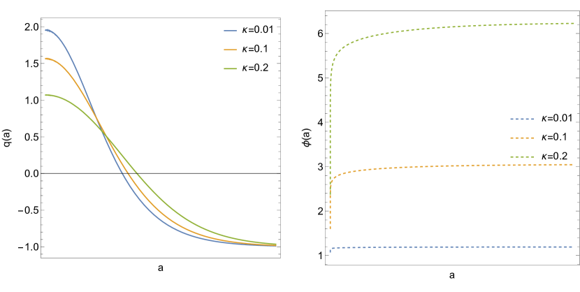
Figure 1: Qualitative evolution for the deceleration parameter $q\left(a\right)~{}$(Left Fig.) and for the scalar field $\phi\left(a\right)~{}$(Right Fig.) as they are given by the numerical solution for the two-dimensional dynamical system (66), (67). Figures are for negative value of the cosmological constant $\Lambda$ and for positive value for the parameter $\omega_{0}$. The de Sitter universe is an attractor for the dynamical system, while the early universe is described by the scaling solution.

VIII

IX Conclusions

Discrete transformations, which are generalized scale-factor duality symmetries, are studied for the dilaton gravitational Action Integral in the trinity of gravity. The Gasperini-Veneziano scale-factor duality transformation for the scalar-tensor theory is examined within the teleparallelism framework, in the scalar-torsion model, and in the symmetric teleparallel scalar-tensor model. In these theories, the dilaton field is nonminimally coupled to the Ricci scalar $R$, the torsion scalar $T$, or the nonmetricity scalar $Q$, respectively.

In teleparallel and symmetric teleparallel theories, we found families of generalized Gasperini-Veneziano scale-factor duality transformations which keep the gravitational Lagrangians invariant. The Gasperini-Veneziano transformation exists as a limit when the coupling term of the gravitational Lagrangian dominates. Furthermore, we examined the existence of continuous transformations that generate the discrete transformations, and by using Noether’s theorem, we determined the corresponding conservation laws for the dilaton Action in the trinity of gravity.

Finally, the integrability properties of the cosmological models investigated, and we derived a new analytic solution within the symmetric teleparallel scalar-tensor theory. The latter cosmological solution possesses two main epochs for the universe: a scaling solution, which can describe the matter or the radiation era, and an accelerated solution described by a de Sitter universe as a future attractor.

In a future study, we plan to investigate further the physical properties of these models. Moreover, the duality transformation will be applied to investigate the physical properties of spacetime in the pre-big bang epoch by using the late-time behaviour.

References

• (1) A. Giveon, M. Porrati and E. Rabinovici, Phys. Rept. 244, 77 (1994)
• (2) M.A.R Osorio and M.A. Vazquez-Mozo, Phys. Lett. B 320, 259 (1994)
• (3) T.H. Buscher, Phys. Lett. B 194, 59 (1987)
• (4) T.H. Buscher, Phys. Lett. B 201, 466 (1988)
• (5) A.A. Tseytlin, Phys. Lett. B 242, 163 (1990)
• (6) J.H. Schwarz, Nucl. Phys. Lett. B 411, 35 (1994)
• (7) E. Alvarez, L. Alvarez-Gaume and Y. Lozano, Nucl. Phys. Proc. Suppl. 41, 1 (1995)
• (8) D.S. Berman, D.C. Thompson, Phys. Reports 566, 1 (2015)
• (9) M. Gasperini and G. Veneziano, Astropart. Phys. 1, 317 (1993)
• (10) V. Faraoni, Cosmology in Scalar-Tensor Gravity, Fundamental Theories of Physics vol. 139, Kluwer Academic Press: Netherlands, (2004)
• (11) R. Brustein, M. Gasperini and G. Veneziano, Phys. Lett. B 431, 277 (1998)
• (12) M. Gasperini and G. Veneziano, Phys. Rept. 373, 1 (2003)
• (13) M. Gasperini and G. Veneziano, JHEP 2023, 144 (2023)
• (14) A. Shapere and W. Wilczek, Nucl. Phys. B 320, 609 (1989)
• (15) P. Brax, Rep. Prog. Phys. 81, 016902 (2018)
• (16) J. Yoo and Y. Watanabe, Int. J. Mod. Phys. D 21, 1230002 (2012)
• (17) J.B. Jimenez, L. Heisenberg and T.S. Koivisto, Universe 5, 173 (2019)
• (18) J. Erdmenger, B. Heß, R. Meyer and I. Matthaiakakis, Phys. Rev. D 110, 066002 (2024)
• (19) J.B. Jimenez and T.S. Kovisto, Phys. Rev. D 105, L021502 (2022)
• (20) Y. Carlonia and O. Luongo, arXiv:2410.10935
• (21) L. P. Eisenhart, “Non-Riemannian Geometry”, American Mathematical Society, Colloquium Publications Vol. VIII, New York, (1927)
• (22) K. Hayashi and T. Shirafuji, Phys. Rev. D 19, 3524 (1979)
• (23) M. Hohmann, Phys. Rev. D 104, 124077 (2021)
• (24) A. Paliathanasis, Eur. Phys. J. Plus 136, 674 (2021)
• (25) M. Rocek and E. Verlinde, Nucl. Phys. B 373, 630 (1992)
• (26) E. Alvarez, L. Alvarez-Gaume, J.L.F. Barbon and Y. Lozano, Nucl. Phys. B 415, 71 (1994)
• (27) C.H Brans and R.H. Dicke, Phys. Rev. 124, 925 (1961)
• (28) A.A. Kehagias and A. Lukas, Nuc. Phys. B 477, 549 (1996)
• (29) A. Paliathanasis, S. Capozziello, Mod. Phys. Lett. A 32, 1650183 (2016)
• (30) G. Gionti S.J. and A. Paliathanasis, Mod. Phys. Lett. A 33, 1850093 (2018)
• (31) U. Camara da Silva, A.L. Alves Lima and G.M. Sotkov, JHEP 11, 090 (2016)
• (32) A. Einstein 1928, Sitz. Preuss. Akad. Wiss. p. 217; ibid p. 224 [Translated by A. Unzicker and T. Case, (preprint: arXiv: physics/0503046)]
• (33) K. Hayashi and T. Shirafuji, Phys. Rev. D 19, 3524 (1979)
• (34) R. Ferraro and F. Fiorini, Phys. Rev. D 75, 084031 (2007)
• (35) C.-Q. Geng, C.-C. Lee, E.N. Saridakis and Y.-P. Wu, Phys. Lett. B 704, 384 (2011)
• (36) A. Paliathanasis, Universe 7, 244 (2021)
• (37) D.J. Raine, Rep. Prog. Phys. 44, 1151 (1981)
• (38) L. Järv, M. Rünkla, M. Saal and O. Vilson, Phys. Rev. D 97, 124025 (2018)
• (39) V. Gakis, M. Krššák, J.L. Said and E.N. Saridakis, Phys. Rev. D 101, 064024 (2020)
• (40) J. B. Jimenez, L. Heisenberg and T. Koivisto, Phys. Rev. D 98, 044048 (2018)
• (41) J. B. Jimenez, L. Heisenberg, T. Sebastian Koivisto and S. Pekar, Phys. Rev. D 101, 103507 (2020)
• (42) S.A. Narawade, S.H. Shekh, B. Mishaa, W. Khyllep, J. Dutta, Eur. Phys. J. C 84, 773 (2024)
• (43) L. Pati, B. Mishra and S.K. Tripathy, Phys. Scripta 96, 105003 (2021)
• (44) W. Khyllep, A. Paliathanasis and J. Dutta, Phys. Rev. D 103, 103521 (2021)
• (45) A. Paliathanasis, Phys. Dark Univ. 43, 101410 (2024)
• (46) N. Dimakis, K.J. Duffy, A. Giacomini, A. Yu. Kamenschik, G. Leon and A. Paliathanasis, Phys. Dark Univ. 44, 101436 (2024)
• (47) F. D’ Ambrosio, L. Heisenberg and S. Kuhn, Revisiting cosmologies in teleparallelism, Class. Quantum Grav. 39 025013 (2022)
• (48) N. Dimakis, A. Paliathanasis, M. Roumeliotis and T. Christodoulakis, Phys. Rev. D 106, 043509 (2022)
• (49) L. Heisenberg and M. Hohmann, Eur. Phys. J. C 84, 462 (2024)
• (50) D.A. Gomes, J.B. Jimenez, A.J. Cano and T.S. Koivisto, Phys. Rev. Lett. 132, 141401 (2024)
• (51) M.-J. Guzman, L. Järv and L. Pati, arXiv:2406.11621 (2024)
• (52) A.G. Bello-Morales, J.B. Jimenez, A.J. Caro, A.L. Maroto and T.S. Koivisto, arXiv:2406.19355 (2024)
• (53) A. Paliathanasis, Annals Phys. 468, 169724 (2024)
• (54) M. Tsamparlis and A. Paliathanasis, Symmetry 10, 233 (2018)