Ridge Regression for Manifold-valued Time-Series with Application to Meteorological Forecast

Abstract

We propose a natural intrinsic extension of the ridge regression from Euclidean spaces to general manifolds, which relies on Riemannian least-squares fitting, empirical covariance, and Mahalanobis distance. We utilize it for time-series prediction and apply the approach to forecast hurricane tracks and their wind speeds.

1 Introduction

We use intrinsically defined polynomials to model manifold-valued time-series. To this end, we utilize the extension of the ordinary de Casteljau algorithm and the resulting Bézier curves to manifolds, presented in [22] and [20]. The latter also proposes some basic properties and presents applications to motion of rigid body, space of positive definite matrices, construction of canal and developable surfaces, and curve design on implicit surfaces and polyhedra. Moreover, the mentioned work also extends the ordinary de Boor algorithm, and therewith, Bézier splines (also called composite Bézier curves) to manifolds. Note that, variational splines [6] also offer flexible models, but are computationally more costly. The work [24] characterize manifold-valued polynomials by vanishing higher-order covariant derivative. However, this approach also suffers from high computational cost (polynomials are determined by solving higher-order differential equations involving the curvature tensor). Due to evaluation via de Casteljau algorithm, Bézier polynomials offer high computational efficiency.

We employ a natural extension of the widespread least-squares regression technique to estimate the best-fitting Bézier curves that model the trajectories. We recall that smoothing, dimensional reduction, and suppressing inconsistencies and noise are advantages of regression. For a comprehensive introduction and applications, we refer to [18, 17] and [19], which employed geodesic regression (as a counter part to the ordinary linear one) and [16, 13] for the general case of manifold-valued splines. In the applications, along with the regression, we compute the coefficient of determination to examine the model’s adequacy.

Ridge regression is a popular adaptation of Tikhonov regularization to standard regression to estimate coefficients in the underlying model, especially when independent variables are highly correlated. This method has been used in many fields, including computational science and engineering and econometrics. It often provides prediction efficiency over simple linear regression with a significant number of model parameters, and helps reduce overfitting that can result from model complexity. For an overview, we refer to [15, 12] and [23]. The proposed approach in this work is a natural intrinsic extension of the ridge regression from Euclidean spaces to arbitrary Riemannian manifolds, which incorporates Mahalanobis distance and correlation matrix. It gives rise to prediction for trajectories in the underlying manifold and will be applied to forecast hurricane tracks and intensities (wind speeds).

This work is organized as follows. The next section is devoted to mathematical preliminaries from Riemannian geometry, least-squares technique, the polynomial manifold-valued model and our approach, the ridge regression. In Section 3, we discuss the application of our approach to hurricanes, the modifications and numerical results.

2 Prediction for Trajectories in Riemannian Manifolds

In this section, we provide an overview of our regression model to represent trajectories by best-fitting Bézier curves, and subsequently expose our approach to prediction.

For preliminaries from Riemannian geometry, we refer to [8] and [14]. Let $M$ be a finite-dimensional Riemannian manifold. We denote its Riemannian distance by $dist$, the exponential and its local inverse, the logarithmic maps of $M$ by $\exp$ and $\log$, respectively, and set $I:=[0,1]$. Moreover, we denote the tangent space of $M$ at $x$ by $T_{x}M$, and the number of control points of the best-fitting Bézier curves (polynomials) by $n$, and set $\mathcal{M}:=M^{n}$, $\mathcal{U}:=U^{n}$, where $U$ refers to a normal convex (also called totally normal) neighbourhood in $M$.

2.1 Bézier Polynomials and Regression

Let $b_{1},\cdots,b_{n}$ be points in $U$. Applying the de Casteljau algorithm, defines a polynomial $p(t;b)$ with control points $b_{1},\cdots,b_{n}$. Here $b$ stands for $(b_{1},\cdots,b_{n})$ and $n-1$ is the degree of the polynomial $p(.;b)$. For a comprehensive introduction and some applications in data science, we refer to [16] and the recent overview [13]. Evaluation of the polynomials is, due to the use of the de Casteljau algorithm, computationally very efficient.

We use the widespread least-squares regression technique to estimate the best-fitting (not restricted to interpolatory) Bézier curves that model the trajectories in $M$.

Consider scalars $t_{1}<t_{2}<\cdots<t_{m}$ and sample points $y_{1},\cdots,y_{m}\in U$ of a trajectory $y$, i.e., $y_{i}=y(t_{i})$. Our regression model aims at finding a polynomial $p=p(.;b)$ that best fits the data $(t_{i},y_{i})$ in the least squares sense:

$$\sum_{i=1}^{m}dist^{2}(y_{i},p(t_{i};b))\to\min.$$

The minimizer is the best-fitting polynomial of degree $n-1$ for data $(t_{i},y_{i})$ with $i=1,\cdots,m$. Applying a linear bijection, we may assume that $t_{1}=0$ and $t_{m}=1$. Computationally, we employ the parametrization by the control points to determine the corresponding polynomial $p(.;b^{\ast})$, where $b^{\ast}\coloneqq\operatorname{arg\,min}H$ and

$$H(b):=\sum_{i=1}^{m}dist^{2}(y_{i},p(t_{i};b))$$

The choice $b_{i}=\gamma(\frac{i-1}{n-1})$ with $i=1,\cdots,n$ and $\gamma(t):=\exp_{y_{1}}(t\log_{y_{1}}y_{m})$, serves as a convenient initial guess. The predictive power of the regression model can be measured by the coefficient of determination, denoted $R^{2}$. To compute it, let $H_{min}:=H(b^{\ast})$ and denote the minimum of

$$G(x)\coloneqq\sum_{i=1}^{m}dist^{2}(y_{i},x))$$

by $G_{min}$. We recall that the minimizer of $G$ is the (Fréchet) mean of the points $y_{1},\cdots,y_{m}$. Now, the coefficient of determination reads

$$R^{2}=1-\frac{H_{min}}{G_{min}}.$$

Note that $\frac{1}{m}H_{min}$ and $\frac{1}{m}G_{min}$ are the unexplained and total variances, respectively.

2.2 Ridge Regression

Next, we propose our extended ridge regression. This approach, adapting a Tikhonov regularization to our parametric regression, allows prediction building on the polynomial model function. To this end, we utilize the notions of covariance and Mahalanobis distance, extended from Euclidean spaces to general manifolds (cf. the survey [21]). The regularizer has the geometric interpretation of Mahalanobis distance to the fitted prior data.

We denote the Riemannian metric of $\mathcal{M}$ by $g$, and its distance, exponential and logarithmic maps by $\mathrm{d}$, $\mathrm{Exp}$ and $\mathrm{Log}$ respectively. Now, fix $\mu\in\mathcal{U}$, a positive definite selfadjoint endomorphism $S$ of $T_{\mu}\mathcal{M}$ and consider the function $F_{\mu,S}:\mathcal{U}\to\mathbb{R}$ defined by

$$F_{\mu,S}(b) =H(b)+g_{\mu}(S\mathrm{Log}_{\mu}b,\mathrm{Log}_{\mu}b).$$

Clearly, we may write

$$g_{\mu}(S\log_{\mu}x,\log_{\mu}x)=g_{\mu}(W\log_{u}x,W\log_{\mu}x)$$

where $W$ is a positive definite endomorphism (in the Euclidean case Tikhonov matrix) on $T_{\mu}\mathcal{M}$. Now, fix $\lambda>0$. We seek to minimize $F_{\mu,\lambda S}$ with $\mu$ the expected value, $S$ the precision, i.e., inverse of the covariance $\Sigma$ of $b$, and a suitably chosen ridge parameter $\lambda$.

2.2.1 Linearization and Gradient

Let $\textnormal{grad}\,F_{\mu,S}$ denote the gradient of $F_{\mu,S}$. If $M$ is Euclidean, then $p(t;b)=Xb$ with a matrix $X$ determined by $(t_{1},\cdots,t_{m})$, and stacking $y_{1},\cdots,y_{m}$ as a vector $y$, a straightforward computation shows that

$$\textnormal{grad}_{b}F_{\mu,S}=X^{T}(Xb-y)+S(b-\mu),$$

implying the following well-known explicit expression for the minimizer of $F_{\mu,S}$

$$b=(X^{T}X+S)^{-1}(X^{T}y+S\mu).$$

Generally, due to absence of an explicit analytic solution, the regression task has to be solved numerically. To this end, we employ a Riemannian steepest descent solver [1]. In this regard, if we do not use automatic differentiation, the main challenge is the computation of the gradient of $F_{\mu,S}$. It has been shown in [4, Sec. 4.2] that $\textnormal{grad}\,H$ can be computed as the adjoint of the sum of certain Jacobi fields (in closed form, if $M$ is a symmetric space). We still need to determine the gradient of the squared Mahalanobis distance. For this purpose, we have the following result.

Proposition 1

Consider the function $f$ defined on $\mathcal{U}$ by

$$f(x)=g_{\mu}(S\mathrm{Log}_{\mu}x,\mathrm{Log}_{\mu}x).$$

Fix $x\in U$. Let $\gamma$ be the geodesic given by $\gamma(t)=\mathrm{Exp}_{\mu}(t\mathrm{Log}_{\mu}x)$ with $t\in I$. Let $J$ be the Jacobi field along $\gamma$ with $J(0)=0$ and $\dot{J}(0)=S\mathrm{Log}_{\mu}x$ (dot stands for derivative with respect to $t$). Then

$$\textnormal{grad}_{x}f=2J(1).$$

Let $k$ be the function defined by $k(x)=\mathrm{Exp}_{\mu}(W\mathrm{Log}_{\mu}x)$ on $U$, and denote the tangent map of $k$ evaluated at $x$ by $d_{x}k$. Then

$$\textnormal{grad}_{x}f=-2(d_{x}k)^{*}(\mathrm{Log}_{k(x)}\mu),$$

where the superscript * represents the adjoint.

Proof

Fix $v\in T_{x}\mathcal{M}$. Denoting the differential map of $f$ at $x$ by $d_{x}f$, we have the following.

$$d_{x}fv =g_{\mu}(Sd_{x}\mathrm{Log}_{\mu}v,\mathrm{Log}_{\mu}x)+g_{\mu}(S\mathrm{Log}_{\mu}x,d_{x}\mathrm{Log}_{\mu}v)$$

$$=2g_{\mu}(S\mathrm{Log}_{\mu}x,d_{x}\mathrm{Log}_{\mu}v)$$

$$=2g_{x}(d_{\mathrm{Log}_{\mu}x}\mathrm{Exp}_{\mu}(S\mathrm{Log}_{\mu}x),d_{\mathrm{Log}_{\mu}x}\mathrm{Exp}_{\mu}(d_{x}\mathrm{Log}_{\mu}v)),$$

where the last equation follows from the Gauß lemma. Now, $\mathrm{Exp}_{\mu}(\mathrm{Log}_{\mu})$ is the identity on $\mathcal{U}$, hence we have $d_{\mathrm{Log}_{\mu}x}\mathrm{Exp}_{\mu}(d_{x}\mathrm{Log}_{\mu}v)=v$ and arrive at

$$d_{x}fv =2g_{x}(d_{\mathrm{Log}_{\mu}x}\mathrm{Exp}_{\mu}(S\mathrm{Log}_{\mu}x),v).$$

Hence

$$\textnormal{grad}_{x}f=2d_{\mathrm{Log}_{\mu}x}\mathrm{Exp}_{\mu}(S\mathrm{Log}_{\mu}x).$$

Now, let $\epsilon>0$ be small enough, such that the image of the map $C$ given by

$$C(\tau,t):=\mathrm{Exp}_{\mu}(t(\mathrm{Log}_{\mu}x+\tau S\mathrm{Log}_{\mu}x)),\>(\tau,t)\in\,]-\epsilon,\epsilon[\times I,$$

is in $\mathcal{U}$. The map $C$ is a variation of $\gamma$ through geodesics, and the vector field $J$ defined by $J(t)=\partial_{\tau}C(0,t)$ the Jacobi field along $\gamma$ with $J(0)=0$ and $\dot{J}(0)=S\mathrm{Log}_{\mu}x$. Due to [14, Sec. 5.2]

$$d_{\mathrm{Log}_{\mu}x}\mathrm{Exp}_{\mu}(S\log_{\mu}x)=J(1),$$

which immediately implies the first desired formula. Now, consider the function $r$ defined by $r=d^{2}(\mu,.)$ on $U$. We have $f(x)=r(k(x))$. Thus,

$$d_{x}fv =d_{k(x)}r(d_{x}kv)$$

$$=g_{k(x)}(\textnormal{grad}_{k(x)}r,d_{x}kv)$$

$$=g_{x}((d_{x}k)^{*}(\textnormal{grad}_{k(x)}r),v)$$

and the well-known formula $\textnormal{grad}_{y}r=-2\mathrm{Log}_{y}\mu$ with $y=k(x)$ completes the proof.

We remark that if $M$ is embedded in some Euclidean space, than the gradient can also be obtained by projecting the Euclidean one to the tangent space at the point of the evaluation.

2.2.2 Mahalanobis Distance and Fitting Data

Let $B$ denote a set of samples $b^{1},\cdots,b^{l}$ from a probability distribution in $\mathcal{M}$ with mean $\mu$. The matrix $\frac{1}{l-1}\sum_{j=1}^{l}\log_{\mu}b^{j}(\log_{\mu}b^{j})^{T}$ (the superscript $T$ represents the transpose) in exponential chart at $\mu$ defines an endomorphism $\Sigma$ on $T_{\mu}\mathcal{M}$, which is independent of the coordinates (cf. [21]). Thus, $\Sigma$ extends the the notion of ordinary Euclidean (sample) covariance matrix to general Riemannian manifolds. Its inverse $S:=\Sigma^{-1}$ is the precision operator. The squared Mahalanobis distance between $B$ and an arbitrary point $x\in M$ denoted by $d_{Mah}$ reads

$$d_{Mah}^{2}(B,x) =g_{\mu}(S\mathrm{Log}_{\mu}x,\mathrm{Log}_{\mu}x).$$

Now, let $j=1,\cdots,l$ and consider a set $Y$ of discrete trajectories (not necessarily with equal sample sizes) $y^{j}$ in $M$ and $B$ be the set of corresponding control points $b^{j}=(b_{1}^{j},\cdots,b_{n}^{j})\in\mathcal{M}$ of the best-fitting polynomials for the trajectories, gained by minimizing $H$. Now, we may write

$$F_{\mu,\lambda S}(b) =H(b)+\lambda d_{Mah}^{2}(B,b).$$

Thus, $F_{\mu,\lambda S}$ averages the least-squares regression using $H$ given in the previous subsection and the squared Mahalanobis distance to $B$.

2.2.3 Parameter Optimization and Forecasting

The ridge parameter $\lambda$ controls the amount of regularization, which aims to achieve a balance between preventing overfitting and accurately predicting the training set. Nonetheless, an excessively high value of $\lambda$ may lead to an underfitted model that is unable to adequately capture significant patterns within the dataset. Therefore, it is important to determine an optimal value for $\lambda$.

Now, fix $\lambda$ and initial samples $y_{1},\cdots,y_{i-1}$ of a discrete trajectory not in the prior. We aim to predict $y_{i}$. Our initial prediction reads $\hat{y}_{i}:=p(t_{i};b_{i}^{\ast})$, where $b_{i}^{\ast}$ denotes the minimizer of $F_{\mu,\lambda S}$. A common issue is that, in general, for coarse sampling as well as for long-term forecasting ($t_{i}-t_{i-1}$ much larger than the preceding time step), the error $d(\hat{y}_{i},y_{i})$ can increase excessively. To account for such effects and fine tuning, we slightly extend our ridge regression by adding a simple and computationally fast averaging step as follows. We replace $\hat{y}_{i}$ with $\exp_{y_{i-1}}\hat{y}_{i}$. Note that for $\alpha=1$, $\hat{y}_{i}$ remains unchanged. Iteration over $i$ yields the initial prediction for the whole trajectory. The initial and final values of $i$ are application dependent.

Our next task is to find optimal values for the parameter $\lambda$ and $\alpha$. To this end, one can use the well-known methods in the Euclidean case such as cross-validation. Thereby, denoting the validation dataset by $\tilde{Y}$, optimal parameter values $(\lambda^{\ast},\alpha^{\ast})$ can be gained iteratively via minimization of the residual

$$\sum_{\tilde{y}=(\tilde{y}_{1},\cdots,\tilde{y}_{m})\in\tilde{Y}}\sum_{i=i_{0}}^{m}d^{2}(\hat{y}_{i},\tilde{y}_{i}).$$

Obviously, the choice of the prior and its splitting in $\tilde{Y}$ and $Y$ depends on the application and particularly, properties like seasonality and relevance of historical order of the trajectories. Moreover, using a larger prior requires more computation time and memory. However, it does not necessarily result in better prediction accuracy on the test dataset. On the other hand, it is unlikely to achieve satisfactory prediction accuracy with smaller $Y$ and $\tilde{Y}$.

3 Application: Hurricanes Forecast

Tropical cyclones, also known as hurricanes or typhoons, are among the most powerful natural phenomena with enormous environmental, economic, and human impact. The most common indicator of a hurricane’s intensity is its maximum sustained wind speed, which is used to categorize the storm on the Saffir-Simpson hurricane wind scale. For example, wind speeds $\geq 137$ knots correspond to category 5. High track variability and out-most complexity of hurricanes has led to a large number of works to classify, rationalize and predict them. We remark that many approaches are not intrinsic and use linear approximations. We refer to the overview [10], the summary of recent progress [7], and [11].

3.1 Dataset

We verify the effectiveness of the proposed framework by applying it to the Atlantic hurricane data from the HURDAT 2 database provided by the U.S. National Oceanic and Atmospheric Administration, publicly available on https://www.nhc.noaa.gov/data/. The data comprise measurements of latitude, longitude, and wind speed on a 6 hours base. The sample size (number of points that make up a track) varies from 13 to 96. Minimum of observed wind speeds is $15$ knots. Fig. 1 illustrates this dataset depicting the 2021 tracks together with their intensities.

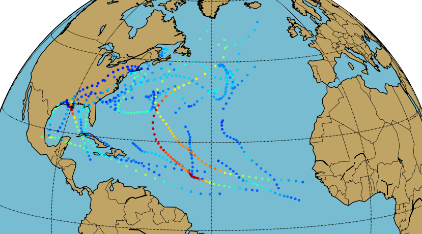
Figure 1: 2021 Atlantic tracks and their intensities (maximum wind speeds).

3.2 Experiments and Discussion

In our experiments, following the verification rules of the U.S. National Hurricane Center (NHC), we computed the average of the MAE (mean absolute error; using spherical distance for the tracks) of the 2021 Atlantic forecasts for comparison. To this end, we represented the tracks and intensities as discrete trajectories in $S^{2}$ and $\mathbb{R}$, respectively. We recall that the Riemannian exponential and logarithmic maps for $S^{2}$ read as follows.

$$\exp_{x}v =\cos(\varphi)\cdot x+\frac{\sin(\varphi)}{\varphi}\cdot v,$$

$$\mathrm{Log}_{x}y =\varphi\frac{y-\langle x,y\rangle x}{\|y-\langle x,y\rangle x\|},$$

where $x,y\in S^{2}$ with $dist(x,y)<\pi$ and $v$ orthogonal to $x$ with length $\varphi$ ($\exp_{x}0=x$). We initiated each forecast using the first sample (initial value of $i$ was $2$) and choose $n=6$, resulting in average $R^{2}$ values $>0.85$ for both fitted tracks and intensities. Fig. 2 shows two example tracks with their representation in our polynomial regression model.

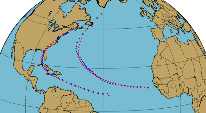
Figure 2: Two exemplary tracks (blue) with their representation (red) in our polynomial regression model.

We employed two experiments, Exp1 and Exp2. Due to the deviations of annual trends and relevance of the chronological order, in Exp1, we used the 2020 ones (31 trajectories) as prior and the last 21 for validation to forecast all the 2021 ones (21 trajectories), and in Exp2, the first 16 trajectories from 2021 as prior with its last 5 trajectories to forecast the last 5 trajectories. It turned out that while the intensities are highly correlated, the covariance matrix of the tracks is almost singular. We solved the latter issue employing diagonal loading (simple standard approach to numerically treat matrices having determinant close to zero, i.e., $\approx$ machine precision; cf. [5]). Higher values of $n$ increased the forecast error of the tracks (overfitting due to small position correlations). For parameter optimization we only employed a simple rough grid search to decrease the computation time (on average few seconds for each forecast). Variations in the settings with significantly larger or smaller validation sets increased the errors, and as expected, validation sets chronologically closer to the test sets resulted in forecasts with slightly higher accuracies.

Obviously, one can model the tracks as images of the Euclidean best-fitting polynomials in geographic coordinates (in the latitude-longitude plane) under the standard parametrization of the sphere. Our computations show that this increases errors, demonstrating the advantage of our intrinsic approach. Figure 3 shows an example with a particularly large track error, which is mainly caused by the loop. The increase in error due to the presence of a loop, in addition to metheological anomalies, is an issue known in other approaches (cf.  [2]).

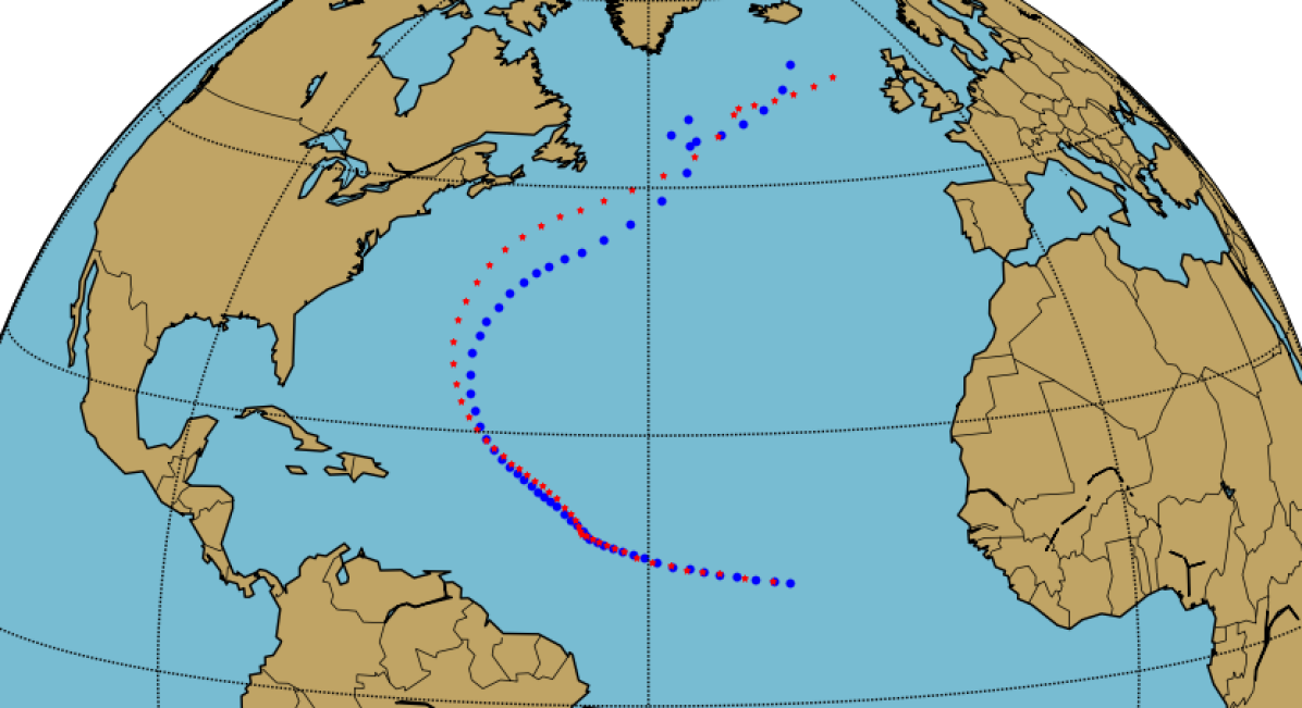
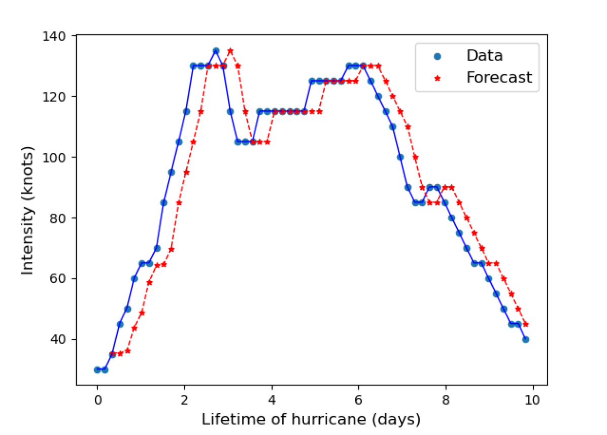
Figure 3: 12 h forecasts (red) via ridge regression for the category 4 and long-lasting 2021 hurricane Sam (blue).

Of course, we did not expect results very close to those of NHC, since our approach is generic and does not include all the relevant physical parameters, while NHC uses several more elaborate physical models. The average 12 h forecast errors of the standard NHC model OCD5 (cf. [9]) and our two primary experiments regarding the Atlantic basin for the 2021 season are summarized in table  1.

Table 1: Average 12 h forecast errors of NHC/OCD5 model and proposed approach in the Atlantic basin for the 2021 (Exp1: all, Exp2: last 5) cyclones

Experiment/Method	Intensities (kt)	Tracks (mi)
Exp1/NHC	6.4	48.2
Exp1/Proposed	6.9	90.7
Exp2/NHC	7.5	67.4
Exp2/Proposed	6.5	97.2

For the code implementing our approach, which in particular includes Riemannian optimization for the computation of geodesic paths and Bézier polynomials, we used the publicly available Python package morphomatics v4.0 (cf. [3]).

4 Conclusion

In this work, we presented an intrinsic natural extension of polynomial ridge regression, respectively, Tikhonov regularization, from Euclidean spaces to arbitrary Riemannian manifolds. This allows for the prediction of manifold-value time series using the Mahalanobis distance to the training data as a prior. We also provided formulae for computing the gradient of the loss function in the approach. In addition, we provided a discussion of our numerical experiments on the application of the approach to hurricane forecasting and intensity.

There are several exciting tasks for future work. First, we plan to consider further data-driven modifications to improve our results on hurricanes, especially with respect to long-term forecasts. Particularly, a joint representation in $S^{2}\times\mathbb{R}$ to incorporate position-intensity correlation is natural. We also plan to consider further applications and apply our approach to morphology and shape analysis. As another example application, and to exploit the effect of negative curvature, we plan to study the Hadamard manifold of positive definite symmetric matrices, which is of both application and theoretical importance.

4.0.1 Acknowledgements

The author is supported through the DFG individual funding with project ID 499571814.

References

- [1] Absil, P.A., Mahony, R., Sepulchre, R.: Optimization Algorithms on Matrix Manifolds. Princeton University Press, Princeton, NJ, USA (2007), http://www.manopt.org
- [2] Alemany, S., Beltran, J., Perez, A., Ganzfried, S.: Predicting hurricane trajectories using a recurrent neural network. In: Proceedings of the AAAI Conference on Artificial Intelligence. vol. 33, pp. 468–475 (2019)
- [3] Ambellan, F., Hanik, M., von Tycowicz, C.: Morphomatics: Geometric morphometrics in non-Euclidean shape spaces (2021). https://doi.org/10.12752/8544, https://morphomatics.github.io/
- [4] Bergmann, R., Gousenbourger, P.Y.: A variational model for data fitting on manifolds by minimizing the acceleration of a Bézier curve. Front. Appl. Math. Stat. 4, 1–16 (2018). https://doi.org/10.3389/fams.2018.00059
- [5] Besson, O., Vincent, F.: Performance analysis of beamformers using generalized loading of the covariance matrix in the presence of random steering vector errors. IEEE Transactions on Signal Processing 53(2), 452–459 (2005)
- [6] Camarinha, M., Silva Leite, F., Crouch, P.E.: High-order splines on riemannian manifolds. Proceedings of the Steklov Institute of Mathematics 321, 158–178 (2023). https://doi.org/0.1134/S0081543823020128
- [7] Cangialosi, J.P., Blake, E., DeMaria, M., Penny, A., Latto, A., Rappaport, E., Tallapragada, V.: Recent progress in tropical cyclone intensity forecasting at the national hurricane center. Weather and Forecast. 35(5), 1913–1922 (2020). https://doi.org/10.1175/WAF-D-20-0059.1
- [8] do Carmo, M.P.: Riemannian Geometry. Mathematics: Theory and Applications, Birkhäuser Boston, Cambridge, MA, USA, 2 edn. (1992)
- [9] Center, A.N.H.: National hurricane center forecast verification report 2021 (2021), https://www.nhc.noaa.gov/verification/pdfs/Verification_2021.pdf
- [10] Chen, R., Zhang, W., Wang, X.: Machine learning in tropical cyclone forecast modeling: A review. Atmosphere 11(7) (2020). https://doi.org/10.3390/atmos11070676
- [11] DeMaria, M., Franklin, J.L., Zelinsky, R., Zelinsky, D.A., Onderlinde, M.J., Knaff, J.A., Stevenson, S.N., Kaplan, J., Musgrave, K.D., Chirokova, G., Sampson, C.R.: The national hurricane center tropical cyclone model guidance suite. Weather and Forecasting 37(11), 2141 – 2159 (2022). https://doi.org/10.1175/WAF-D-22-0039.1
- [12] Golub, G.H., Hansen, P.C., O’Leary, D.P.: Tikhonov regularization and total least squares. SIAM journal on matrix analysis and applications 21(1), 185–194 (1999)
- [13] Hanik, M., Nava-Yazdani, E., von Tycowicz, C.: De casteljau’s algorithm in geometric data analysis: Theory and application. Computer Aided Geometric Design 110, 102288 (2024). https://doi.org/10.1016/j.cagd.2024.102288
- [14] Jost, J.: Riemannian Geometry and Geometric Analysis. Universitext, Springer (2011). https://doi.org/10.1007/978-3-642-21298-7
- [15] McDonald, G.C.: Ridge regression. WIREs Computational Statistics 1(1), 93–100 (2009). https://doi.org//10.1002/wics.14
- [16] Nava-Yazdani, E., Ambellan, F., Hanik, M., von Tycowicz, C.: Sasaki metric for spline models of manifold-valued trajectories. Computer Aided Geometric Design 104, 102220 (2023). https://doi.org/10.1016/j.cagd.2023.102220
- [17] Nava-Yazdani, E., Hege, H.C., Sullivan, T.J., von Tycowicz, C.: Geodesic analysis in kendall’s shape space with epidemiological applications. Journal of Mathematical Imaging and Vision pp. 1–11 (2020). https://doi.org/10.1007/s10851-020-00945-w
- [18] Nava-Yazdani, E., Hege, H.C., von Tycowicz, C.: A geodesic mixed effects model in kendall’s shape space. In: Multimodal Brain Image Analysis and Mathematical Foundations of Computational Anatomy, pp. 209–218. Springer (2019). https://doi.org/10.1007/978-3-030-33226-6_22
- [19] Nava-Yazdani, E., Hege, H.C., von Tycowicz, C.: A hierarchical geodesic model for longitudinal analysis on manifolds. Journal of Mathematical Imaging and Vision 64(4), 395 – 407 (2022). https://doi.org/10.1007/s10851-022-01079-x
- [20] Nava-Yazdani, E., Polthier, K.: De Casteljau’s algorithm on manifolds. Comput. Aided. Geom. Des. 30(7), 722–732 (2013). https://doi.org/10.1016/j.cagd.2013.06.002
- [21] Pennec, X.: Intrinsic statistics on riemannian manifolds: Basic tools for geometric measurements. Journal of Mathematical Imaging and Vision 25, 127–154 (2006)
- [22] Popiel, T., Noakes, L.: Bézier curves and interpolation in Riemannian manifolds. J. Approx. Theory 148(2), 111–127 (2007). https://doi.org/10.1016/j.jat.2007.03.002
- [23] Shalabh: Theory of Ridge Regression Estimation with Applications. Journal of the Royal Statistical Society Series A: Statistics in Society 185(2), 742–743 (02 2022). https://doi.org/10.1111/rssa.12816
- [24] Singh, N., Hinkle, J., Joshi, S., Fletcher, P.T.: A hierarchical geodesic model for diffeomorphic longitudinal shape analysis. In: International Conference on Information Processing in Medical Imaging. pp. 560–571. Springer (2013)