Multi-response linear regression estimation based on low-rank pre-smoothing

Abstract

Pre-smoothing is a technique aimed at increasing the signal-to-noise ratio in data to improve subsequent estimation and model selection in regression problems. However, pre-smoothing has thus far been limited to the univariate response regression setting. Motivated by the widespread interest in multi-response regression analysis in many scientific applications, this article proposes a technique for data pre-smoothing in this setting based on low-rank approximation. We establish theoretical results on the performance of the proposed methodology, and quantify its benefit empirically in a number of simulated experiments. We also demonstrate our proposed low-rank pre-smoothing technique on real data arising from the environmental and biological sciences.

Keywords low-rank approximation  $\cdot$ multi-response model  $\cdot$ parameter estimation  $\cdot$ prediction  $\cdot$ pre-smoothing

1 Introduction

In multivariate data analysis, a common task in analyzing multi-response data is to model the relationships between the vector of responses of interest and a number of explanatory variables. Such data are observed in a multitude of scientific applications, including ecology (Anderson and Underwood, 1997), genetics (Sivakumaran et al., 2011; Liu and Calhoun, 2014), chemometrics (Skagerberg et al., 1992; Burnham et al., 1999), bioinformatics (Kim et al., 2009), population health (Bonnini and Borghesi, 2022), as well as economics and finance (Gospodinov et al., 2017; Petrella and Raponi, 2019). Whilst component-wise analysis may be an option, analyzing each component separately fails to consider the dependence between the components of the responses; this can result in estimators of model parameters that are less efficient than those that account for potential correlation between responses (see e.g. Srivastava and Solanky (2003); Izenman (2008)), and thus multivariate linear models are often more appropriate. See Anderson (2003) for a comprehensive introduction to classical parametric models. Parameter estimation in classical multiresponse regression settings is achieved with the ordinary least squares (OLS) estimator, with the Gauss-Markov theorem showing this estimator to be the best linear unbiased estimator (BLUE) (Johnson et al., 2007, Chapter 7).

In many analysis settings, the mean squared error (MSE) criterion is commonly used to measure of the quality of a prediction technique, incorporating the well-known bias-variance trade-off in assessing estimators. One way to achieve a smaller MSE in univariate regression settings is to use so-called presmoothing, in which response data is smoothed in some way prior to estimation via OLS (Faraldo-Roca and González-Manteiga, 1987; Cristobal et al., 1987; Janssen et al., 2001). The intuition behind this approach is that this first step increases the signal-to-noise ratio in the data, thus reducing the variance contribution in the bias-variance trade-off and consequently reducing parameter uncertainty. Other authors have also noted that pre-smoothing can also help with model selection in uni-response regression (Aerts et al., 2010). The pre-smoothing paradigm has subsequently been used in other modelling settings, such as with functional data (Hitchcock et al., 2006, 2007; Ferraty et al., 2012), as well as semi-parametric and survival models (Musta et al., 2022; Tedesco et al., 2023; Musta et al., 2024). Despite these contributions, pre-smoothing has not been explored in the multi-response regression setting.

In this article, we propose an alternative to the OLS estimator for multi-response regression models using data pre-smoothing, in the spirit of Cristobal et al. (1987); Janssen et al. (2001) in the one-dimensional setting. In what follows, we illustrate this methodology with a low-rank approximation to achieve the pre-smoothing, hence we term our proposed technique low-rank pre-smoothing (LRPS). Our proposed low-rank pre-smoothing technique is naturally “model-free” in the sense that it does not need additional covariate information such as the nonparametric pre-smoothers proposed in the one-dimensional setting, see also the examples of Aerts et al. (2010, Section 2.3). We investigate how LRPS can be used in the linear regression setting, and demonstrate that it achieves a lower MSE than the OLS estimator and shows particular improvements when the number of responses is large, or the signal-to-noise ratio is small.

This article is structured as follows. In Section 2, we provide a detailed description of our low rank pre-smoothing estimator. In particular, the theoretical properties of the estimator are explored in Section 2.1. We then present the results of the simulation studies in Section 2.3 to examine the effectiveness of the proposed LRPS estimator. We illustrate the practical use of our proposed method in prediction tasks of real data arising in biology and environmental science in Section 4. Finally, we make some concluding remarks in Section 5.

2 Low-rank pre-smoothing in multivariate regression

Consider the multivariate multiple outcome linear regression model

$$Y=XB+E\;,$$ (1)

where $Y=(y_{1},\ldots,y_{n})^{\top}$ and $E=(e_{1},\ldots,e_{n})^{\top}$ are $n\times q$ dimensional random matrices representing the outcomes and errors respectively. We study the fixed design case whereby $X\in\mathbb{R}^{n\times p}$, and $B\in\mathbb{R}^{p\times q}$ are parameters to be estimated. We further assume that $e_{i}$ is independent from $e_{j}$ for all $j\neq i$, where $i,j=1,2,\dots,n$ and has constant covariance $\mathrm{Cov}(e_{i})=\Sigma_{e}$. In the case where $e_{i}\overset{iid}{\sim}N_{q}(0,\Sigma_{e})$, the model (1) can be alternatively written as

$$\mathrm{vec}(Y)\sim\mathcal{N}_{pq}\left(\mathrm{vec}(XB),\Sigma_{e}\otimes I_{p}\right).$$ (2)

When $n>p$ the maximum-likelihood estimator for $B$ under (2) is well defined, and is given by the OLS solution $\hat{B}=S_{X}^{-1}S_{XY}$ where $S_{X}=n^{-1}X^{\top}X$ and $S_{XY}=n^{-1}X^{\top}Y$. This estimator has the distributional property (see e.g., Mardia et al. (1995, Chapter 6)) that

$$\mathrm{vec}(\hat{B})\sim\mathcal{N}_{pq}(\mathrm{vec}(B),n^{-1}\Sigma_{e}\otimes S_{X}^{-1})\;,$$ (3)

and as a consequence, the estimator is consistent and unbiased (Greene, 2018, Chapter 4).

Whilst asymptotically the OLS maintains the best unbiased linear estimate (BLUE) properties, the $pq$ dimensional quantity $\mathrm{vec}(B)$ is still relatively high-dimensional. As such, performance in finite samples may result in noisy estimates, with considerable variance. The aim of this paper is to propose an estimator that enjoys superior finite-sample (and asymptotic) performance when estimating $B$. Our proposal is straightforward, and aims to reduce the proportion of the noise, i.e. variance of errors, that contributes to the regression problem at hand. We now formally define our proposed estimator.

Definition 1.

LRPS Estimator

Let $S_{Y}=n^{-1}Y^{\top}Y$ and consider its eigendecomposition $\hat{V}\hat{D}\hat{V}^{\top}=S_{Y}$. The Low-Rank Pre-Smoothing (LRPS) estimator for $B$ is then given by

$$\tilde{B}=S_{X}^{-1}S_{XY}\hat{V}_{k}{\hat{V}_{k}}^{\top}\;,$$ (4)

where $\hat{V}=(\hat{V}_{k},\hat{V}_{\backslash k})$, with $\hat{V}_{k}=(\hat{v}_{1},\ldots,\hat{v}_{k})$ being the first $k\leq q$ eigenvectors, and $\hat{V}_{\backslash k}$ the remaining $q-k$ eigenvectors. We assume the ordering of $k$ matches that of the eigenvalues $\hat{D}=\mathrm{diag}(\hat{d}_{1},\ldots,\hat{d}_{q})$ and $\hat{d}_{k}\geq\hat{d}_{k+1}$.

The LRPS estimator can be seen as the OLS estimator applied to a “pre-smoothed” set of outcomes $\tilde{Y}=Y\hat{W}_{k}$, with $\hat{W}_{k}=\hat{V}_{k}{\hat{V}_{k}}^{\top}$ acting to project $Y$ onto the subspace spanned by $\hat{V}_{k}$, and then ${\hat{V}_{k}}^{\top}$ projecting back into the original dimensions of $Y$. The estimator is simple to compute, with the truncated eigenvectors $\hat{V}_{k}$ found in $\mathcal{O}(kq^{2})$ computational time. Furthermore, via the Eckhardt-Young theorem (Jolliffe and Cadima, 2016) we have that $\tilde{Y}$ is the best rank $k$ approximation of $Y$ under the least-squares (Frobenius) loss. The method is feasible as $\hat{V}_{k}$ are the empirical eigenvectors associated with the observed $Y$, and not on a population, or model-dependent quantity. Our motivation is somewhat similar to that of Cristobal et al. (1987); Janssen et al. (2001) who propose non-parametric pre-smoothing of an outcome before performing the regression. However, in our case, we have a multi-outcome (multivariate) setting, and the smoothing is performed via a specific device, that is the projection onto the most influential eigenvectors of the outcome. We note here that other suitable multivariate non-parametric data smoothers could be used for pre-smoothing, however, they would need other (covariate) information as inputs to the smoother, and potentially suffer from the curse of dimensionality in high-dimensional multi-response data regimes.

At this point, we should note that a similar methodology can be employed within the class of methods known as reduced rank-regression (Izenman, 1975). We elaborate on the similarities and differences between LRPS and these methods later in Section 2.2, however as the name suggests, reduced rank-regression aims to find a low-rank approximation of $B$, whereas LRPS makes no such explicit assumption, and indeed, we can set $k\geq\min(n,p)$ in LRPS to enable $\tilde{B}$ to remain full rank. A further difference between the methods is that LRPS doesn’t require knowledge of $X$ prior to choice of eigenvectors, as $V_{k}$ are obtained directly from $Y$. However, the optimal choice of $k$ will in general depend on the shape of the spectrum (eigenvalues) of $XB$, $E$, and the dimensionality $p,n,q$. This aspect of our proposed method is explored further in Section 3.

2.1 Theoretical properties of the LRPS estimator

In this section, we discuss the asymptotic distribution for the LRPS estimator and the potential efficiency gains relative to OLS. Our analysis is in the standard dimensional setting where $p,q$ are assumed fixed, and we let $n\rightarrow\infty$. To study the estimator in this setting, we consider the population covariance $\Sigma_{y}=n^{-1}(XB)^{\top}(XB)+\Sigma_{e}=B^{\top}S_{X}B+\Sigma_{e}$, its eigendecomposition $\Sigma_{y}=VDV^{\top}$, and the smoothing operator $W_{k}=V_{k}{V_{k}}^{\top}$ based on the first $k$ eigenvectors.

Theorem 1.

Asymptotic Distribution of LRPS

Under model (1), suppose the moments of the errors $\{e_{1},\ldots,e_{n}\}$ exist (and are finite) up to the fourth order. Assuming that $\lim_{n\rightarrow\infty}S_{X}=\Sigma_{X}$, then we have

$$n^{1/2}\mathrm{vec}\left(\tilde{B}-BW_{k}\right)\stackrel{{\scriptstyle D}}{{\rightarrow}}\mathcal{N}_{pq}\left(\mathbf{0},W_{k}\Sigma_{e}W_{k}\otimes\Sigma_{x}^{-1}\right)\;,$$ (5)

as $n\rightarrow\infty$.

The proof of the above can be found in A, and relies on the consistency of the sample eigenvectors $\mathrm{plim}_{n\rightarrow\infty}\hat{V}_{k}=V_{k}$, where $\mathrm{plim}$ denotes as convergence in probability (Neudecker and Wesselman, 1990; Bura and Pfeiffer, 2008). The result shows $\tilde{B}$ is a root-$n$ consistent estimator of the corresponding low-rank projection of $B$, $BW_{k}$; furthermore, this illustrates that whilst the LRPS estimator may be a biased estimator of the coefficient matrix $B$ (for $k<q$), it enjoys better mean squared error (MSE) performance than the OLS in some important scenarios.

Let $\mathrm{MSE}(\tilde{B}):=\mathbb{E}_{E}(\|\tilde{B}-B\|_{F}^{2})$ where we take expectations over the error matrix $E$ with $n$ rows and $q$ columns, e.g. as in the model (1). For a large $n$, if the asymptotic distribution of Theorem 1 held, the MSE of LRPS can be approximated as

$$\mathrm{MSE}(\tilde{B})\approx\underset{\mathrm{Var}(\tilde{B})}{\underbrace{\frac{\bar{\alpha}_{X}}{n}\mathrm{Tr}(\hat{W}_{k}\Sigma_{e})}}+\underset{\mathrm{Bias}^{2}(\tilde{B})}{\underbrace{\mathrm{Tr}\{(I_{q}-\hat{W}_{k})B^{\top}B\}}},$$ (6)

where $\bar{\alpha}_{X}:=\mathrm{Tr}(S_{X}^{-1})$. The first term represents the variance of the estimator, and the second, the square of the bias.

Note that the form of the mean squared error expression in (6) is, as expected, dependent on the chosen number of low rank components, $k$. This recovers the MSE for the OLS when $k=q$, in which case the bias disappears as $\hat{W}_{q}=I_{q}$. The variance reduction relative to OLS is given by

$$\frac{\mathrm{Var}(\tilde{B})}{\mathrm{Var}(\hat{B})}\approx\frac{\|\Sigma_{e}^{1/2}\hat{V}_{k}\|_{F}^{2}}{\|\Sigma_{e}^{1/2}\|_{F}^{2}}\leq\frac{\sum_{i=1}^{k}\gamma_{i}^{2}(\Sigma_{e}^{1/2})}{\sum_{i=1}^{q}\gamma_{i}^{2}(\Sigma_{e}^{1/2})}\;,$$

thus if the spectrum of the errors is relatively flat, then the reduction can be of order $k/q$, a substantial benefit when $q$ is large. On the other hand, if the spectrum of the errors is spiked, e.g. if $\Sigma_{e}$ were geometrically decaying, then the variance reduction benefits of LRPS may be minimal. In terms of bias, we see this is related to the proportion of the signal (as expressed via $B$ through $X$) into the orothocomplement of the space spanned by the first $k$ singular vectors of $Y$. The eigenvectors $\hat{V}_{k}$ will in general not be optimal for representing the signal $XB$, however, are chosen based on a combination of this signal, and the error $EV_{k}$.

2.2 Relation to Reduced-Rank-Regression

In the case when $k\leq\min(p,n)$ it is of interest to understand the performance of LRPS in terms of estimation bias, in particular, in comparison to reduced-rank-regression (RRR) methods (Izenman, 1975; Reinsel et al., 2022) which aims to solve the problem

$$\bar{B}\in\operatorname{argmin}_{B\in\mathbb{R}^{p\times q}}\|Y-XB\|_{F}^{2}\qquad\mathrm{s.t.}\;r(V)\leq k\;,$$

for a given $k\leq\min(p,q)$, where $r(V)$ denotes the rank of $V$. A classical approach to this problem is to minimise $B$ after projecting onto the space spanned by the rank-$k$ approximation of $\hat{Y}=HY$ where $H=n^{-1}XS_{X}^{-1}X^{\top}$.

Definition 2.

Reduced-Rank Regression

Consider the decomposition:

$$U_{k}G_{k}{U_{k}}^{\top}+U_{\backslash k}G_{\backslash k}U_{\backslash k}^{\top}=\frac{1}{n}Y^{\top}HHY=\hat{B}^{\top}S_{X}\hat{B}\;,$$

where $U_{k},G_{k}$ are matrices representing the first $k$ eigenvectors and eigenvalues of the decomposition respectively. The Reduced-Rank Regression (RRR) estimator is then defined as

$$\bar{B}=S_{X}^{-1}S_{XY}U_{k}{U_{k}}^{\top}\;.$$ (7)

The form of the estimator follows from noting that when $n>p$ we have

$$\bar{B}=\arg\min_{r(B)\leq k_{*}}\{\|Y-X\hat{B}\|_{F}^{2}+\|XB-X\hat{B}\|_{F}^{2}\}\;.$$

Applying Theorem 2.1 in Reinsel et al. (2022) to optimize over the second term in the equation above leads to (7). We thus see that LRPS and RRR are closely related, the difference being the choice of basis used in the projection step. When $n>p$, then RRR represents the optimal solution in the Gaussian error setting (where it attains the MLE and thus BLUE property), when the low-rank $k_{*}=r(B)\leq\min(q,p)$ assumption holds. Importantly, our proposed LRPS method can also be applied when $k\geq p$, whereas RRR falls back to the OLS solution (for $k\geq\min(p,q)$ we obtain $\bar{B}=\hat{B}U_{k}{U_{k}}^{\top}=\hat{B}$). In this setting, RRR and OLS may have high-variance, whilst LRPS can still benefit from variance reduction. We now provide some initial insight into the scenarios in which the Teo estimators differ.

2.3 Empirical Analysis and Finite-Sample Behaviour

To give some intuition on the differences between the three estimators, LRPS, RRR, and OLS, we consider a simple simulation study in which we empirically track the MSE, the bias, and the variance of the estimators as a function of $k$. We consider two scenarios, one where the true rank $r(B)=k_{*}=p/2$ is small relative to $\min(p,q)$, and the other where $k_{*}=\min(p,q)$. For simplicity, we let $p=q=10$, $k_{*}=\{5,10\}$ and consider three sample sizes $n=\{20,30,50\}$ to assess the finite-sample behaviour of the estimators. In each case we assume the model (2), we simulate $X$ and $E$ as a set of isotropic Gaussian random vectors (independent rows). Further details on the simulation design can be found in Section 3, where we present results from a more comprehensive study.

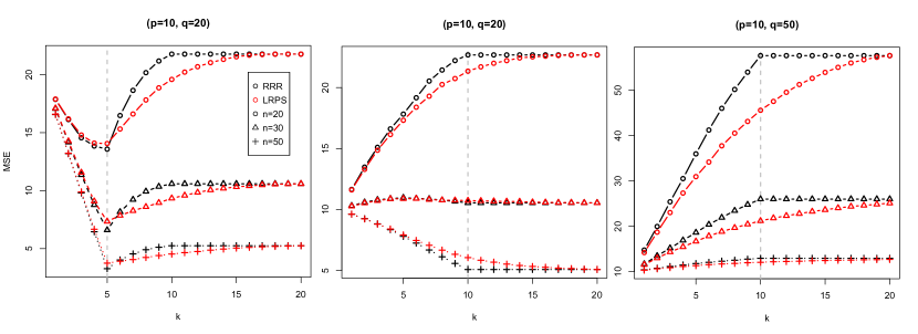
Figure 1: Performance of LRPS and RRR in terms of empirical $\mathrm{\hat{MSE}=}m^{-1}\sum_{s=1}^{m}\|Y^{(s)}-X^{(s)}B^{(s)}\|_{F}^{2}$ where $Y^{(s)},X^{(s)}$ and $B^{(s)}$ represent the data, and estimate (LRPS in red, and RRR in black) for simulation $s$, and $m=100$ is the number of simulations.

The results in Figure 1 shed some light on the similarities and differences between LRPS and RRR. When the true model is low-rank, e.g. when $k_{*}=5$, we see that for all sample sizes the minimum MSE is attained at $r(\bar{B})=k_{\star}$ and RRR performs slightly better in terms of estimation error at this minimum. On the other hand, when the low-rank assumption no longer holds ($k_{*}=10$), we see that LRPS outperforms RRR in the small sample size setting, whereas RRR becomes superior as the sample size $n$ grows. Indeed, in the small sample setting, a rank-1 approximation is preferred by both approaches, however, LRPS still maintains better performance. In the scenario where $q$ is large relative to $p$ (Figure 1, right panel), LRPS exhibits superior estimation performance in the full-rank scenario, consistently over a range of sample sizes. This latter point is important as the setting where $q>p$ often occurs in practice. For instance, this is often observed in datasets from air pollution monitoring stations, where measurements of several pollutants are collected across multiple locations. This is discussed later in our application of LRPS to real data.

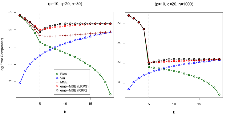
Figure 2: The $\mathrm{bias}^{2}(\tilde{B})$, $\mathrm{Var}(\tilde{B})$, and $\mathrm{MSE}(\tilde{B})$ values extrapolated from the LRPS asymptotic distribution in Theorem 1, compared to the finite-sample (empirical) MSE for both LRPS and RRR. In this simulation, $k_{*}=5$ and other than the sample size, the conditions are the same as those given in the left pane of Figure 1.

A characteristic property of LRPS is that the estimator responds to changes in $k_{*}>\min(p,q)$, whereas RRR falls back to the OLS estimator in this regime. To investigate the bias-variance tradeoff occurring due to the pre-smoothing we plot the $\mathrm{bias}^{2}(\tilde{B})$, $\mathrm{Var}(\tilde{B})$, and $\mathrm{MSE}(\tilde{B})$ components from (6), and compare them with the empirical MSE achieved in a finite sample, in this case, letting $n=30$ and $n=1000$. The results are presented in Figure 2. As one may expect, extrapolating from the asymptotic to the finite sample setting may not be appropriate for small samples, but the approximation becomes tighter as $n$ increases. Comparing the dark red (+) and red ($\times$) lines in Figure 2, we note that they essentially overlap in the larger $n=1000$ setting. We now provide more insight into the performance of LRPS through in-depth simulations.

3 Simulation Study

In this section, we evaluate the performance of our proposed technique by using simulated examples to assess the estimation of the regression coefficient matrix, as well as out-of-sample predictive performance. The data $Y,X$ are simulated according to (1), where we fix the design of the covariates to be $X\sim\mathcal{N}_{n\times p}(0,I_{p}\otimes I_{n})$. we vary the specification of the true coefficient matrix $B$, and the covariance structure of the errors $\Sigma_{e}$. The choices here cover a range of scenarios that are of interest in practice and help further elucidate the behaviour of LRPS (and RRR) when the spectrum (eigenstructure) of the signal $XB$ and noise $E$ vary. The various conditions for $B$ and $\Sigma_{e}$ are given below.

Coefficient Matrix Conditions:

1 - Sparse and low-rank: Let $s$ be the expected rank of the coefficient matrix. We first select active elements for $B^{\prime}_{ij}$ by sampling from the Bernoulli distribution, $B^{\prime}_{ij}\sim\text{Bernoulli}(s^{-1})$ for $j=1,\ldots,s$. The non-zero coefficients in each row are then scaled (by dividing by the row-average) to maintain $\|B_{i,\cdot}\|_{2}=1$.

2 - Dense and unknown rank: Two random matrices $A_{L}\in\mathbb{R}^{p\times p},A_{R}\in\mathbb{R}^{q\times q}$ are generated with standard normal, and $\text{Uniform}(0,1)$ entries respectively. Let $L$ and $R$ be the left and right singular vectors of $A_{L}$ and $A_{R}$, then the coefficient matrix is then generated according to

$$B=A_{L}\mathrm{diag}(d_{1},\ldots d_{\min(p,q)})A_{R}^{T}\;,$$

where $d_{i}=\lambda^{i}$ exhibits geometric decay.

3 - Dense and known rank: The matrix $B$ is constructed as in Condition 2, however, the diagonal singular values are replaced with $d_{i}=\lambda$ for $i=1,\ldots,k_{*}$ and $d_{i}=0$ for $k_{*}+1,\ldots,\min(p,q)$. This creates a matrix which has rank $k_{*}$. Note, the examples demonstrated in Section 2.3 also use matrices generated in this manner.

Noise Conditions:

1 - Isotropic IID noise: The covariance of the errors is given by $\Sigma_{e}=\sigma^{2}I_{q}$.

2 - Geometric Decaying Toeplitz: We let $\Sigma_{e}=\mathrm{Toeplitz}(\rho)$ such that $\Sigma_{e;i,j}=\sigma^{2}\rho^{|i-j|}$.

Note that simulations in this section as well as the examples in Section 2.3 were produced in the R statistical computing environment (R Core Team, 2024).

3.1 Estimation Error Results

This section examines the estimation error incurred by LRPS and RRR in the scenarios described above. As in the previous section, we focus on understanding the performance of the methods over a range of $k$, and examine how this performance is dependent on the composition of the signal and noise. For simplicity, we fix $n=100$ and report performance as measured by the empirical mean squared error from the true coefficient matrix $B$, averaged across $m=100$ experiments.

Large $q$, moderate $p$

In this case, we consider when $q=100>p=10$ and thus the range of $k$ with which we can apply LRPS is extended relative to RRR (which we recall limits $k\leq\min(p,q)$). In this scenario, we should expect that the structure of the error covariance plays a key role, and given the number of outcomes, the regression problem inherits a lower signal-to-noise as $\|\Sigma_{e}\|_{F}\asymp q$ whilst $\|XB\|_{F}\asymp\sqrt{pq}$. We run three experiments in this setting:

• The first probes what we may expect to happen if $B$ were sparse, under B condition 1. In this case, the rank of the matrix is bounded by $s$, which we choose to be $p/2=5$, since sparsity is a common assumption in high-dimensional regression, we wanted to investigate how methods that previously would focus explicitly on a low-rankness assumption can also be applied in this setting.

• Second, we investigate the case where $B$ is dense, but with decaying singular values (Condition 2), and we consider $\lambda=\{0.9,0.5,0.2\}$ to study the impact of the decay rate.

• Third, we examine the impact of a spiked error covariance via a geometrically decaying correlation structure with values $\rho=\{0.9,0.5,0.2\}$. The specification of $B$ is given via Condition 3 with a flat spectrum ($\lambda=1$).

The last two experiments fix $\sigma^{2}=1$, whereas the first fixes the design of $B$ and varies $\sigma^{2}=\{0.5,1,2\}$ to directly investigate the impact of the error variance on estimation performance. Figure 3 summarises the distribution of $\gamma_{j}^{2}(B)$ and $\gamma_{j}(\Sigma_{e})$, where for each $j=1,\ldots q$ we take the average over $m=100$ experiments.

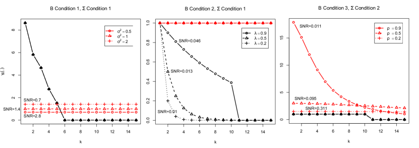
Figure 3: Distribution of singular values for the signal $\gamma_{j}(B)$ and noise $\gamma_{j}^{1/2}(\Sigma_{e})$, in black and red respectively. The signal-to-noise ratio $\mathrm{SNR}:=\|XB\|_{F}/\|\Sigma_{e}\|_{F}$ is given next to each line, and the lines represent the average value of the spectrum over $m=100$ simulations.

The results of the experiment are presented in Figure 4, with experiments 1–3 running from left to right. The figure shows a range of empirical behaviours for the RRR and LRPS estimators and illustrates both estimators’ potential benefits beyond the OLS estimation. The best rank approximation, i.e. the $k$ which minimises the estimation error is a function of both the specification of the signal (via $B$), and the noise structure—in general, a higher signal-to-noise ratio mandates the choice of a smaller $k$. Intuitively, this observation makes sense, as in the high-noise settings, we should desire to constrain the estimator more to avoid excessive variance, i.e. the variance reduction benefits of the low-rank projection dominate the error. Observe, at least when $q>p$, that LRPS is often superior to RRR in these approximations, e.g. when comparing the rank-1 approximation performance in the middle and right plots.

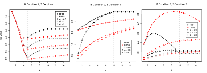
Figure 4: Comparison of LRPS and RRR performance as a function of $k$ in the case where $p=10$, $q=100$, $n=100$. Black lines denote the performance of RRR and red those of LRPS. In the middle and right plots, we fix $\sigma^{2}=1$ and vary the eigenvalues of the signal and noise respectively by adjusting $\lambda$ and $\rho$. In $B$ Condition 3, we set all the singular values of $B$ to be one, and maintain that $r(B)=p$ indicated by the dashed line, in the left plot, we set the sparsity to be $s=5$.

Moderate $q$, Large $p$

In contrast to the high $q$ setting, in this simulation we investigate the relatively high-dimensional estimation problem where $q=10$ is fixed and we set $p\in\{20,40,60\}$, we fix the sample size at $n=100$. In this situation the true rank is limited to be less than or equal to $q=10$, specifically, we simulate $B$ matrices according to Condition 3, and set the rank $k_{*}=5$. We vary the SNR according by adopting $\Sigma$-Condition 1, and letting $\sigma^{2}\in\{0.5,1,2\}$. The results of the experiment are seen in Figure 5. We see that both RRR and LRPS perform well relative to the OLS, and whilst RRR outperforms LRPS for $k\leq k_{*}$ the difference between the two estimators is small. In this case, the best approximating model, i.e. the $k$ which minimises the MSE, depends not only on the SNR mediated by $\sigma^{2}$, but also the variance in the estimators due to the higher number of covariates $p>q$. As $p$ approaches $n$ from below, we see that again the rank-1 approximation achieves best performance for both LRPS and RRR. These results highlight the importance of performing the pre-smoothing (projection) to reduce noise, either when the dimensionality of covariates is high, and/or when the SNR is low. Generally when $k\geq\hat{k}=\arg\min_{k}\mathrm{MSE}(k)$ we see that LRPS outperforms RRR, and the difference in performance can be substantial in the large $q$ setting.

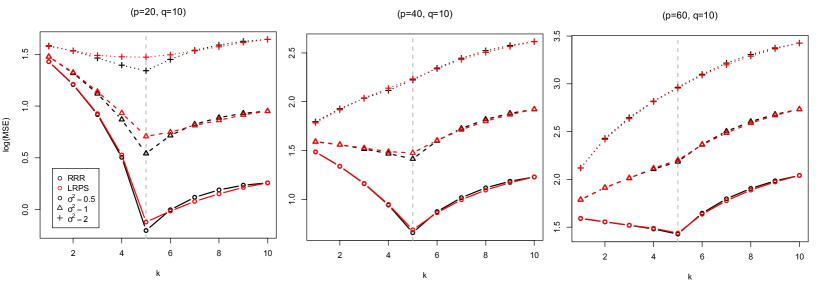
Figure 5: Comparison of LRPS and RRR performance as a function of $k$ in the case where $q=10$, $n=100$ and $p\in\{20,40,60\}$. The covariance of errors is given by $\Sigma$-Condition 1 with $\sigma^{2}\in\{0.5,1,2\}$, the true rank of $B$ is denoted by the vertical grey line.

3.2 Predictive Performance

In both the case of LRPS and RRR we see that the choice of $k$ is important. In this section, we demonstrate the effectiveness of cross-validation for choosing this $k$, and further evaluate the predictive performance of the LRPS and RRR estimators, in an out-of-sample setting.

In general, the selection of how strong we wish our constraints to be in statistical inference may depend on the task at hand. For example, in the lasso ($\ell_{1}$ regularised regression), if one wishes to perform an optimal selection of non-zero coefficients, the specification of the regularisation (constraint) may be different from that for producing optimal predictions. In that setting, typically cross-validation will overestimate the support of the regression function compared to more conservative information criteria. Moving back to the rank-restricted setting with RRR and LRPS, we may encounter a similar position—that is, do we construct an information criterion for the selection of $k$, or do we use some in-sample empirical measure of prediction error, e.g. cross-validation. As we are focussing on global constraints (i.e. working with linear projections across all variates), we here focus on predictive performance rather than parametric inference when deciding the appropriate specification of $k$, and to this end, adopt a simple cross-validation procedure.

Specifically, we propose to apply 2-fold cross-validation, such that we minimise

$$\mathrm{cvMSPE}(k):=\frac{1}{2}\left(\|Y^{(1)}-X^{(1)}\hat{B}^{(2)}W_{k}^{(2)}\|_{F}^{2}+\|Y^{(2)}-X^{(2)}\hat{B}^{(1)}W_{k}^{(1)}\|_{F}^{2}\right)\;,$$ (8)

where $Y^{(1)}$ indicates data obtained from the first half of the data and $Y^{(2)}$ the second half of the data. Note, we use the eigenvectors from the corresponding training dataset, i.e., $W_{k}^{(j)}=V_{k}^{(j)}V_{k}^{(j)\top}$ are based on the first $k$ singular vectors of $Y^{(j)}\in\mathbb{R}^{\frac{1}{2}n\times q}$, where $j\in\{1,2\}$. The $\mathrm{cvMSPE}(k)$ function can be regarded as an in-sample estimate of the out-of-sample prediction error, and if the generating process is stationary, this will be a consistent estimator of this quantity as $n\rightarrow\infty$.

In the following experiments, we consider the estimates $\hat{k}$ according to

$$\hat{k}=\arg\min_{k=1,2,\ldots}\mathrm{cvMSPE}(k)$$

for both RRR and LRPS. Note, the version stated in (8) can be readily applied to RRR by simply replacing $V_{k}$ with $U_{k}$ (from Definition 2). To evaluate the performance of the selection criteria, we consider the empirical distribution of $\hat{k}$ alongside the out-of-sample expected prediction error $\mathbb{E}_{(y^{\prime},x^{\prime})}\|y^{\prime}-x^{\prime}\hat{B}V_{\hat{k}}V_{\hat{k}}^{\top}\|_{F}^{2}$ where $y^{\prime},x^{\prime}$ are assumed to be generated from the same generating process that generated the training data, i.e. $y^{\prime}\sim\mathcal{N}_{q}(0,B^{\top}\Sigma_{X}B+\Sigma_{E})$ and $x^{\prime}\sim\mathcal{N}_{p}(0,I_{p})$.

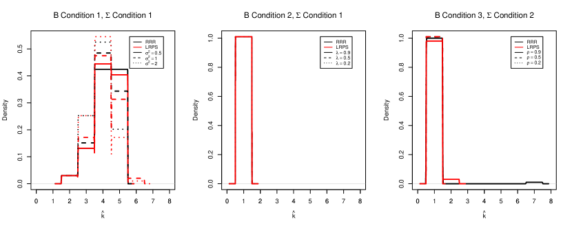
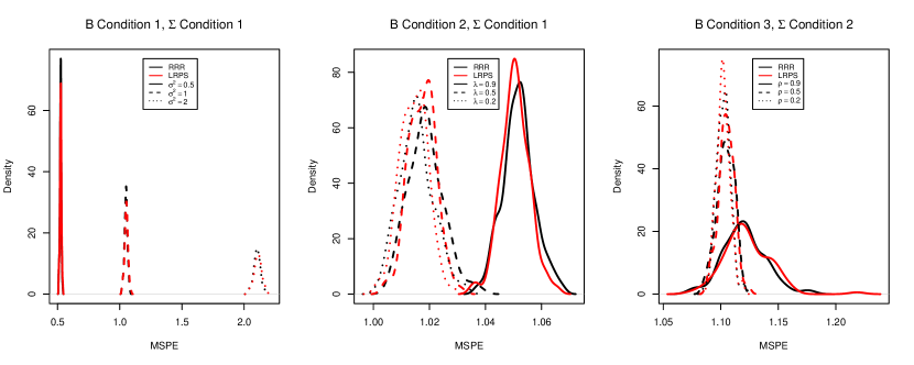
Figure 6: Top: Distribution of $\hat{k}$ (chosen by 2-fold cross-validation); Bottom: Distribution of prediction error. Both distributions are estimated across $100$ replications. Prediction error is based on applying the singular vectors from the training set $n=100$ to the out-of-sample data. The simulation settings mirror those in Figures 3 and 4, with RRR given by the black lines, and LRPS given by those in red.

The results of our experiment are presented in Figure 6. The simulation settings are exactly the same as those considered in Figure 4. In this case, the difference between LRPS and RRR is negligible—both LRPS and RRR estimators appear to adapt its rank (and model complexity) via the proposed cross-validation procedure, i.e. $\hat{k}$ depends on the simulation design (e.g. signal-to-noise ratio, noise/signal distribution).

4 Application to real data

In this section, we demonstrate our proposed LRPS method to study datasets arising from two scientific applications, the first considering air pollution and the second gene activation data.

4.1 Air pollution example

Particulate matter up to $2.5\mu m$ (PM2.5), is a type of air pollution that poses a significant threat to human health and the environment. These tiny particles are made up of a complex mixture of solids, chemicals, and liquid droplets that can penetrate the respiratory system and cause respiratory and cardiovascular problems. It is recognised that controlling such particular matters is of vital importance for the public health (Franck et al., 2011; Pun et al., 2017). In this example, we consider the possible association between PM2.5 emissions and recordings of other pollutant gases, namely: ozone (O3), sulphur dioxide (SO2), carbon monoxide (CO), and nitrogen dioxide (NO2). To study this association, we consider three datasets:

• UK: Pollution across seven cities ($p=7)$ in the United Kingdom (UK). There are daily recordings of the pollutants for a total of $n=400$ data-points, $q=28$ (the number of sites $\times$ number of polluting gases). This data is available from https://uk-air.defra.gov.uk/. We use the first 80% observations $n_{\mathrm{train}}=320$ data points to train the model, and the remaining 20% observations $n_{\mathrm{test}}=80$ for evaluation.

• Beijing: This multi-site air-quality dataset (Liang et al., 2015) can be found at the UCI Machine Learning Repository http://archive.ics.uci.edu/ml/datasets and has been used in the literature in different contexts, e.g. Ma et al. (2022). In this case, we have hourly air pollutant measurements from $p=12$ outdoor monitoring sites in Beijing, collected from March 2013 to February 2017. We focus on the air pollutant measurements for January 2017, resulting in a dataset with $n=743$ ($n_{\mathrm{train}}=594$, $n_{\mathrm{test}}=149$) observations and $q=48$ outcomes. It should be noted that the dataset contains missing values, which for simplicity we replace with the value of the previous detection in the same variable.

• USA: The last dataset is collected from $p=37$ monitoring sites in the United States of America (USA) from January 2017 to April 2019, resulting in a total of $n=728$ ($n_{\mathrm{train}}=578$, $n_{\mathrm{test}}=150$) observations (available from https://www.epa.gov/outdoor-air-quality-data). This is the largest dataset in this study, with $q=148$ outcomes.

For each dataset we take first-differences (across rows of $Y,X$) and standardize all variables so they have mean zero and standard deviation 1. In each case, we estimate the regression parameters $B$ on the training dataset, and tune $k$ via the 2-fold cross-validation procedure employed previously. The remaining $n_{\mathrm{test}}$ data points (20%) are used for evaluation via the mean-square prediction error

$$\text{ MSPE }=\frac{1}{qn_{test}}\left\|X_{\text{test }}\hat{B}-Y_{\text{test }}\right\|_{F}^{2}.$$

The results of the prediction errors and the rank $k$ used in the low-rank pre-smoothing model are presented in Table 1.

Table 1: Prediction error and optimal rank for the pollution datasets described in the main text.

Dataset	Method	Prediction Error (MSPE)	Rank
UK ($p=7,q=28$)	LRPS	0.738	5
	RRR	0.749	6
	OLS	0.751	N/A
Beijing ($p=12,q=48$)	LRPS	1.145	12
	RRR	1.154	6
	OLS	1.175	N/A
USA ($p=37,q=148$)	LRPS	0.911	2
	RRR	0.916	1
	OLS	0.925	N/A

In all cases, LRPS provides better prediction performance than the more traditional approaches. Generally, LRPS and RRR outperform OLS. Whilst the differences in performance are not vast, the results demonstrate that low-rank approximations may generally be useful, and it is interesting that in these cases the rank selected is always lower than $\min(p,q)$. In the case of the USA, we see that the rank selected is $k=1,2$ in RRR and LRPS respectively. This behaviour was seen in our synthetic experiments in the high $q$ setting, e.g. see $B$ Condition 2, $\Sigma$ Condition 1 results in Figure 4.

4.2 Gene association example

In addition to the air pollution datasets, we applied our proposed methodology to a genetic association dataset from Wille et al. (2004). This dataset is from a microarray experiment designed to explore regulatory mechanisms within the isoprenoid gene network of Arabidopsis thaliana, also known as thale cress or mouse-ear cress. Isoprenoids are known to play numerous essential biochemical roles in plants. To track gene expression levels, $n=118$ GeneChip microarray experiments were conducted. The dataset includes $p=39$ predictor genes from two isoprenoid biosynthesis pathways, MVA and MEP, while the response variables consist of the expression of $q=795$ genes across 56 metabolic pathways. To reduce skewness in the distributions, all variables are log-transformed before fitting the linear models. We use the first $n_{\mathrm{train}}=96$ observations as the training set, and then calculate the prediction error using the remaining $n_{\mathrm{test}}=22$ observations.

Table 2: Prediction error and optimal rank for the genetic association dataset described in the main text.

Method	Prediction Error (MSPE)	Rank
LRPS	0.414	2
RRR	0.418	2
OLS	0.481	N/A

The results are presented in Table 2, and demonstrate the benefits of the low-rank approximation similar to the air-pollution dataset. In this case, we have a very large $q$ compared to $p$, and both are relatively large when compared to the number of data-points $n$. It is worth remarking that our holdout dataset in this case is only $n_{\mathrm{test}}=18$ observations, however, the performance is also averaged across the number of outcomes $q=795$ which is relatively large. The analysis here can be considered relatively “high-dimensional” in nature. Both LRPS and RRR choose $k=2$ as the best approximating rank, potentially illustrating behaviour akin to $B$ Condition 1/2 and $\Sigma$ Condition 1 in our synthetic experiments, i.e. where the error spectrum was relatively flat, but the signal was concentrated in terms of the top singular values. Whilst the difference between LRPS and RRR is not large, LRPS maintains the better performance (in-line with the synthetic experiments and the other application), and both low-rank methods considerably outperform OLS.

5 Conclusion

This article proposes Low-Rank Pre-Smoothing, a technique for multi-response regression settings. When viewed as a projection, the method can be seen as an initial step to smooth observed data to increase its signal-to-noise ratio, after which a traditional estimation method such as ordinary least squares (OLS) can be performed for estimation and subsequent prediction. Our technique outperforms the traditional OLS estimator in terms of mean square estimation and out-of-sample prediction error, driven by sacrificing a small amount of bias in favour of reducing the estimation uncertainty. This improved performance was demonstrated through extensive simulated examples, our methodology showing particular benefits when a large number of responses is observed and / or when the signal-to-noise ratio is low. We also illustrated the utility of our proposed methodology on a number of real datasets. Whilst the motivation for the work in this article arose from the classical multi-response setting, we envisage that the tools developed here have the potential to make similar gains in other settings, such as nonlinear regression models, time series forecasting, and high-dimensional penalised data scenarios.

Appendix A Proof of Theorem 1

In this appendix, we provide details of the proof of Theorem 1 described in the main text.

We begin by establishing a result which be useful in the proof of the theorem. Let $Y$ be a random data matrix from model (1) (where the fourth order moments of the errors are finite), $S_{y}=n^{-1}Y^{\top}Y$ the sample covariance matrix, and define $\Sigma_{y}=n^{-1}(XB)^{\top}(XB)+\Sigma_{e}$.

Lemma 1.

Let $S_{y}$ and $\Sigma_{y}$ be as above. Then

$$\sqrt{n}\operatorname{vec}(S_{y}-\Sigma_{y})\stackrel{{\scriptstyle D}}{{\rightarrow}}\mathcal{N}_{q^{2}}\left(0,\mathbf{V}_{y}\right),$$ (9)

where

$$\mathbf{V}_{y}=\mathbb{E}\left[ee^{\top}\otimes ee^{\top}\right]-\operatorname{vec}\left(\Sigma_{e}\right)\otimes\operatorname{vec}\left(\Sigma_{e}\right)$$ (10)

in which $e\in\mathbb{R}^{q\times 1}$ denotes a generic row of $E$.

Proof.

Denote by $S_{e}=n^{-1}E^{\top}E$ the sample covariance of the error vectors $E$ with corresponding population covariance matrix $\Sigma_{e}$. Since the fourth order moments of the error distribution are assumed finite and the rows of $E$ are assumed to be independent and identically distributed under model (1), Theorem 1 in Neudecker and Wesselman [1990] (with zero mean random variables) establishes that $S_{e}$ is a root-$n$ consistent estimator for $\Sigma_{e}$:

$$\sqrt{n}\operatorname{vec}(S_{e}-\Sigma_{e})\stackrel{{\scriptstyle D}}{{\rightarrow}}\mathcal{N}_{q^{2}}\left(0,\mathbf{V}_{e}\right),$$ (11)

where

$$\mathbf{V}_{e}=\mathbb{E}\left[ee^{\top}\otimes ee^{\top}\right]-\operatorname{vec}(\Sigma_{e})\otimes\operatorname{vec}(\Sigma_{e})$$

and $e$ is as above.

Let $Z:=n^{-1}(XB)^{\top}(XB)=n^{-1}B^{\top}(X^{\top}X)B\in\mathbb{R}^{q\times q}$ and $W:=n^{-1}(XB)^{\top}E\in\mathbb{R}^{q\times q}$.

Using the linear model (1), the sample covariance matrix of $Y$, $S_{y}$, can be expressed as

$$S_{y}=n^{-1}Y^{\top}Y=n^{-1}\Bigl{(}(XB)^{\top}(XB)+(XB)^{\top}E+E^{\top}(XB)+E^{\top}E\Bigr{)}.$$ (12)

Then

$$\Sigma_{y}:=\mathbb{E}(S_{y})=n^{-1}\Bigl{(}(XB)^{\top}(XB)\Bigr{)}+n^{-1}\mathbb{E}\Bigl{(}(XB)^{\top}E\Bigr{)}+n^{-1}\mathbb{E}\Bigl{(}E^{\top}(XB)\Bigr{)}+\Sigma_{e}.$$

Because $\mathbb{E}(E)=0$ (and thus $\mathbb{E}(W)=0$), this simplifies to

$$\Sigma_{y}=n^{-1}(XB)^{\top}(XB)+\Sigma_{e}.$$ (13)

Then combining (12) and (13), we get

$$\underbrace{\sqrt{n}\operatorname{vec}(S_{y}-\Sigma_{y})}_{C} = \sqrt{n}\operatorname{vec}\left((Z+W+W^{\top}+S_{e})-\Sigma_{y}\right)$$ (14)

$$= \sqrt{n}\operatorname{vec}\left((Z+W+W^{\top}+S_{e})-\left(Z+\Sigma_{e}\right)\right)$$

$$= \underbrace{\sqrt{n}\operatorname{vec}\left((W+W^{\top})\right)}_{(A_{1})}+\underbrace{\sqrt{n}\operatorname{vec}\left(S_{e}-\Sigma_{e}\right)}_{(A_{2})}.$$

Using the properties of the vec operator [Abadir and Magnus, 2005],

$$\operatorname{vec}\left(W\right)=\operatorname{vec}\left(n^{-1}(XB)^{\top}E\right)=\underbrace{\left(I_{q}\otimes n^{-1}(XB)^{\top}\right)}_{A}\operatorname{vec}(E),$$

where $\otimes$ denotes the Kronecker product, so

$$\operatorname{Var}\left(\operatorname{vec}(W)\right) =\operatorname{Var}\left(A\operatorname{vec}(E)\right)=A\operatorname{Var}\left(\operatorname{vec}(E)\right)A^{\top}$$

$$=\left(I_{q}\otimes n^{-1}(XB)^{\top}\right)(\Sigma_{e}\otimes I_{n})\left(I_{q}\otimes n^{-1}(XB)^{\top}\right)^{\top}$$

$$=\left(I_{q}\Sigma_{e}I_{q}\right)\otimes\left(n^{-2}(XB)^{\top}I_{n}(XB)\right)$$

$$=\Sigma_{e}\otimes n^{-1}Z,$$

using the transpose and mixed-product properties of the Kronecker product. Assuming that $\lim_{n\rightarrow\infty}S_{X}=\Sigma_{x}$ (where $S_{X}=n^{-1}X^{\top}X$) for some fixed positive definite matrix $\Sigma_{x}$ (as is customary in regression), we have

$$\mathbb{E}\left(\operatorname{vec}(W)\right) =0\quad\textrm{and}$$

$$\operatorname{Var}\left(\operatorname{vec}(W)\right) =\Sigma_{e}\otimes n^{-1}Z=\left(\Sigma_{e}\otimes n^{-1}B^{\top}S_{X}B\right)\rightarrow 0.$$

Hence considering the first term $A_{1}$ in (14), we have

$$\operatorname{vec}\left((W+W^{\top})\right)=\left(\operatorname{vec}(W)\right)+\left(\operatorname{vec}(W^{\top})\right)\stackrel{{\scriptstyle\mathbb{P}}}{{\rightarrow}}0$$

thus considering (14) and using (the multivariate version of) Slutsky’s theorem (see e.g., [Cramér, 1999, Section 20.6]), we have

$$\sqrt{n}\operatorname{vec}(S_{y}-\Sigma_{y})\stackrel{{\scriptstyle D}}{{\rightarrow}}\mathcal{N}_{q^{2}}(0,\mathbf{V}_{y}),$$

with

$$\mathbf{V}_{y}=\mathbb{E}\left[ee^{\top}\otimes ee^{\top}\right]-\operatorname{vec}\left(\Sigma_{e}\right)\otimes\operatorname{vec}\left(\Sigma_{e}\right).$$

∎

We now present a theorem and a corollary without proof, both taken from Bura and Pfeiffer [2008], which are used as intermediary results to establish Theorem 1.

Theorem.

Let $\hat{\Omega}$ be a $p\times q$-dimensional random matrix that is a function of a random sample of $p$-dimensional data ${Z_{1},\dots,Z_{n}}$. Assume that $\hat{\Omega}_{n}$ is asymptotically normally distributed as

$$\sqrt{n}\operatorname{vec}(\hat{\Omega}_{n}-\Omega)\stackrel{{\scriptstyle D}}{{\rightarrow}}\mathcal{N}_{pq}(0,\mathbf{V}).$$

Let $r=rank(\Omega)$ with $d\leq\min(p,q)$, and let the singular value decomposition of $\Omega$ be

$$\Omega=L^{\top}\left(\begin{array}[]{ll}D&0\\ \mathbf{0}&0\end{array}\right)R,$$

where $L^{\top}=\left(L_{1},L_{0}\right)$ is of order $p\times p$ with $L_{1}:p\times r$, $L_{0}:p\times(p-r)$. $R^{\top}=\left(R_{1},R_{0}\right)$ is orthogonal with $R_{1}:q\times r,R_{0}:q\times(q-r)$. The $r$ left singular vectors $U_{1}$ of $\Omega$ correspond to its $r$ non-zero singular values, $d_{1}\geq\dots\geq d_{r}$. Analagously, the SVD of $\hat{\Omega}$ is

$$\hat{\Omega}=\hat{L}^{\top}\left(\begin{array}[]{cc}\hat{D}_{1}&\mathbf{0}\\ &\\ \mathbf{0}&\hat{D}_{0}\end{array}\right)\hat{R},$$ (15)

with $\hat{L}^{\top}=\left(\hat{L}_{1},\hat{L}_{0}\right),\hat{R}^{\top}=\left(\hat{R}_{1},\hat{R}_{0}\right)$, and the partition conforms with the partition of $\Omega$.

Assume that $\lambda_{r}>\epsilon>0$, i.e. the minimum positive singular value of $\Omega$ is well separated from zero. Then as $n\rightarrow\infty$

1. $\hat{D}_{1}\stackrel{{\scriptstyle\mathbb{P}}}{{\rightarrow}}D_{1}$ and $\hat{D}_{0}\stackrel{{\scriptstyle\mathbb{P}}}{{\rightarrow}}0$.

2. $\hat{R}_{1}\stackrel{{\scriptstyle\mathbb{P}}}{{\rightarrow}}R_{1}$ and $\hat{L}_{1}\stackrel{{\scriptstyle\mathbb{P}}}{{\rightarrow}}L_{1}$.

Corollary.

The matrix $\hat{L}_{1}$ of left singular vectors in (15) is asymptotically normal with

$$n^{1/2}\operatorname{vec}(\hat{L}_{1}-L_{1})\stackrel{{\scriptstyle D}}{{\rightarrow}}N_{pd}\left(\mathbf{0},\mathbf{\Sigma}_{L}\right),$$ (16)

where

$$\mathbf{\Sigma}_{L}=\left(D^{-1}R_{1}^{\top}\otimes I_{p}\right)\mathbf{V}\left(R_{1}D^{-1}\otimes I_{p}\right).$$ (17)

The assumption on the minimum positive singular value ensures that $\Lambda^{-1}$ is bounded, necessary for the proof of the theorem (see Bura and Pfeiffer [2008]).

We now apply the theorem and corollary to our setting.

Let $V\Lambda V^{\top}$ be the compact form SVD of the quantity $\Sigma_{y}$ from Lemma 1 (equivalent to its eigendecomposition since it is positive semi-definite), and suppose $\Sigma_{y}$ has rank $r$. Suppose also that the random matrix $Y$ has the compact form decomposition $Y=\hat{U}\hat{D}\hat{V}^{\top}$, where the diagonal entries of $\hat{D}$ are $\{\hat{d}_{1},\dots,\hat{d}_{r}\}$. Then $S_{y}$ can be written as

$$n^{-1}Y^{\top}Y=n^{-1}\hat{V}\hat{D}\hat{U}^{\top}\hat{V}\hat{D}\hat{U}^{\top}\\ =\hat{V}\hat{\Lambda}\hat{V}^{\top},$$

due to the orthogonality of $\hat{U}$, and where $\hat{\Lambda}=\operatorname{diag}\left(\hat{\lambda}_{1},\hat{\lambda}_{2},\ldots,\hat{\lambda}_{r}\right)$ is a diagonal matrix containing the descending eigenvalues $\hat{\lambda}_{i}=\hat{d}_{i}^{2}/n,i=1,\dots,r$.

Now using the result established in Lemma 1, the asymptotic normality assumption of the theorem is satisfied for $S_{y}$ as an estimator of $\Sigma_{y}$, hence $\hat{\Lambda}\stackrel{{\scriptstyle\mathbb{P}}}{{\rightarrow}}\Lambda$, and the corollary gives that the matrix $\hat{V}$ of eigenvectors of $S_{y}$ are asymptotically normal with

$$n^{1/2}\operatorname{vec}\left(\hat{V}-V\right)\stackrel{{\scriptstyle D}}{{\rightarrow}}N_{qr}\left(\mathbf{0},\mathbf{\Sigma}_{\hat{V}}\right)\quad\textrm{where}\quad\mathbf{\Sigma}_{\hat{V}}=\left(\Lambda^{-1}V^{\top}\otimes I_{q}\right)\mathbf{V}_{y}\left(V\Lambda^{-1}\otimes I_{q}\right).$$

Hence considering the subset of first $k$ eigenvectors and corresponding eigenvalues ($k<r$), we have that

$$n^{1/2}\operatorname{vec}\left(\hat{V}_{k}-V_{k}\right)\stackrel{{\scriptstyle D}}{{\rightarrow}}N_{qk}\left(\mathbf{0},\mathbf{\Sigma}_{\hat{V}_{k}}\right),$$ (18)

with

$$\mathbf{\Sigma}_{\hat{V}_{k}}=\left({\Lambda_{k}}^{-1}{V_{k}}^{\top}\otimes I_{q}\right)\mathbf{V}_{y}\left(V_{k}{\Lambda_{k}}^{-1}\otimes I_{q}\right),$$

where $\hat{V}_{k}$, $V_{k}$ and $\Lambda_{k}$ correspond to the quantities above, curtailed to $k$ eigenvectors / eigenvalues.

In view of the relationship between the LRPS estimator and the OLS estimator $\hat{B}\hat{V}_{k}{\hat{V}_{k}}^{\top}$, we have $\operatorname{vec}\left(\hat{B}\hat{V}_{k}{\hat{V}_{k}}^{\top}\right)=\left(\hat{V}_{k}{\hat{V}_{k}}^{\top}\otimes I_{p}\right)\operatorname{vec}(\hat{B})$, and the corresponding expression with the true eigenvectors also holds.

Now considering the quantity $\operatorname{vec}\left(\hat{V}_{k}{\hat{V}_{k}}^{\top}\right)$, due to the consistency result for $\hat{V_{k}}$ in (18), the continuous mapping theorem (see e.g. Billingsley [2013]) then means that $\hat{V}_{k}{\hat{V}_{k}}^{\top}$ is a consistent estimator of $V_{k}V_{k}^{\top}$, i.e. $\hat{V}_{k}{\hat{V}_{k}}^{\top}\stackrel{{\scriptstyle\mathbb{P}}}{{\rightarrow}}V_{k}V_{k}^{\top}$ (see also the proof of Theorem 1 in Bura and Pfeiffer [2008]). Using the distributional property (3) and applying Slutsky’s theorem gives that

$$n^{1/2}\operatorname{vec}\left(\tilde{B}-BV_{k}{V_{k}}^{\top}\right) = n^{1/2}\operatorname{vec}\left(\hat{B}(\hat{V}_{k}{\hat{V}_{k}}^{\top}-V_{k}{V_{k}}^{\top})+(\hat{B}-B)V_{k}{V_{k}}^{\top}\right)$$

$$\stackrel{{\scriptstyle D}}{{\rightarrow}} \mathcal{N}\left(\mathbf{0},V_{k}V_{k}^{\top}\Sigma_{e}V_{k}V_{k}^{\top}\otimes S_{X}^{-1}\right),$$

where the variance term is derived as

$$\operatorname{Var}\left(\left(V_{k}V_{k}^{\top}\otimes I_{p}\right)\operatorname{vec}(n^{1/2}\hat{B})\right) = \left(V_{k}V_{k}^{\top}\otimes I_{p}\right)n\operatorname{Var}\left(\operatorname{vec}(\hat{B})\right)\left(V_{k}V_{k}^{\top}\otimes I_{p}\right)^{\top}$$

$$= \left(V_{k}V_{k}^{\top}\otimes I_{p}\right)\left(\Sigma_{e}\otimes S_{X}^{-1}\right)\left(V_{k}V_{k}^{\top}\otimes I_{p}\right)$$

$$= V_{k}V_{k}^{\top}\Sigma_{e}V_{k}V_{k}^{\top}\otimes S_{X}^{-1},$$

using the mixed-product property of Kronecker products.

Note that this result will also be valid if the distributional result (3) is asymptotic, as in the case when the error distribution $G$ in the regression model (1) is not Gaussian.

References

- Abadir and Magnus [2005] K. M. Abadir and J. R. Magnus. Matrix Algebra, volume 1. Cambridge University Press, 2005.
- Aerts et al. [2010] Marc Aerts, Niel Hens, and Jeffrey S Simonoff. Model selection in regression based on pre-smoothing. Journal of Applied Statistics, 37(9):1455–1472, 2010.
- Anderson and Underwood [1997] MJ Anderson and AJ Underwood. Effects of gastropod grazers on recruitment and succession of an estuarine assemblage: a multivariate and univariate approach. Oecologia, 109:442–453, 1997.
- Anderson [2003] T. W. Anderson. Introduction to Multivariate Statistical Analysis. Wiley, 3rd edition, 2003.
- Billingsley [2013] P. Billingsley. Convergence of Probability Measures. John Wiley & Sons, 2nd edition, 2013.
- Bonnini and Borghesi [2022] Stefano Bonnini and Michela Borghesi. Relationship between mental health and socio-economic, demographic and environmental factors in the COVID-19 lockdown period-a multivariate regression analysis. Mathematics, 10(18):3237, 2022.
- Bura and Pfeiffer [2008] E Bura and R Pfeiffer. On the distribution of the left singular vectors of a random matrix and its applications. Statistics & Probability Letters, 78(15):2275–2280, 2008.
- Burnham et al. [1999] Alison J Burnham, John F MacGregor, and Roman Viveros. Latent variable multivariate regression modeling. Chemometrics and Intelligent Laboratory Systems, 48(2):167–180, 1999.
- Cramér [1999] H. Cramér. Mathematical Methods of Statistics, volume 26. Princeton University Press, 1999.
- Cristobal et al. [1987] JA Cristobal Cristobal, P Faraldo Roca, and W Gonzalez Manteiga. A class of linear regression parameter estimators constructed by nonparametric estimation. The Annals of Statistics, 15(2):603–609, 1987.
- Faraldo-Roca and González-Manteiga [1987] P Faraldo-Roca and W González-Manteiga. On efficiency of a new class of linear regression estimates obtained by preliminary non-parametric estimation. New Perspectives in Theoretical and Applied Statistics, pages 229–242, 1987.
- Ferraty et al. [2012] Frédéric Ferraty, Wenceslao González-Manteiga, Adela Martínez-Calvo, and Philippe Vieu. Presmoothing in functional linear regression. Statistica Sinica, pages 69–94, 2012.
- Franck et al. [2011] Ulrich Franck, Siad Odeh, Alfred Wiedensohler, Birgit Wehner, and Olf Herbarth. The effect of particle size on cardiovascular disorders-the smaller the worse. Science of the Total Environment, 409(20):4217–4221, 2011.
- Gospodinov et al. [2017] Nikolay Gospodinov, Raymond Kan, and Cesare Robotti. Spurious inference in reduced-rank asset-pricing models. Econometrica, 85(5):1613–1628, 2017.
- Greene [2018] W. H. Greene. Econometric Analysis. Pearson Education India, 8th edition, 2018.
- Hitchcock et al. [2006] David B Hitchcock, George Casella, and James G Booth. Improved estimation of dissimilarities by presmoothing functional data. Journal of the American Statistical Association, 101(473):211–222, 2006.
- Hitchcock et al. [2007] David B Hitchcock, James G Booth, and George Casella. The effect of pre-smoothing functional data on cluster analysis. Journal of Statistical Computation and Simulation, 77(12):1043–1055, 2007.
- Izenman [2008] Alan J Izenman. Modern multivariate statistical techniques, volume 1. Springer, 2008.
- Izenman [1975] Alan Julian Izenman. Reduced-rank regression for the multivariate linear model. Journal of Multivariate Analysis, 5(2):248–264, 1975.
- Janssen et al. [2001] Paul Janssen, Jan Swanepoel, and Noël Veraverbeke. Efficiency of linear regression estimators based on presmoothing. Communications in Statistics-Theory and Methods, 30(10):2079–2097, 2001.
- Johnson et al. [2007] R. A. Johnson, D. W. Wichern, et al. Applied Multivariate Statistical Analysis. Prentice hall Upper Saddle River, NJ, 6th edition, 2007.
- Jolliffe and Cadima [2016] Ian T Jolliffe and Jorge Cadima. Principal component analysis: a review and recent developments. Philosophical Transactions of the Royal Society A: Mathematical, Physical and Engineering Sciences, 374(2065):20150202, 2016.
- Kim et al. [2009] Seyoung Kim, Kyung-Ah Sohn, and Eric P. Xing. A multivariate regression approach to association analysis of a quantitative trait network. Bioinformatics, 25(12):i204–i212, 2009.
- Liang et al. [2015] Xuan Liang, Tao Zou, Bin Guo, Shuo Li, Haozhe Zhang, Shuyi Zhang, Hui Huang, and Song Xi Chen. Assessing beijing’s pm2. 5 pollution: severity, weather impact, apec and winter heating. Proceedings of the Royal Society A: Mathematical, Physical and Engineering Sciences, 471(2182):20150257, 2015.
- Liu and Calhoun [2014] Jingyu Liu and Vince D Calhoun. A review of multivariate analyses in imaging genetics. Frontiers in Neuroinformatics, 8:29, 2014.
- Ma et al. [2022] Xiaoyan Ma, Qin Zhou, and Xuemin Zi. Multiple change points detection in high-dimensional multivariate regression. Journal of Systems Science and Complexity, 35(6):2278–2301, 2022.
- Mardia et al. [1995] K. V. Mardia, J. T. Kent, and J. M. Bibby. Multivariate Analysis. Probability and Mathematical Statistics. Academic Press, San Diego, 10th edition, 1995.
- Musta et al. [2022] Eni Musta, Valentin Patilea, and Ingrid Van Keilegom. A presmoothing approach for estimation in the semiparametric Cox mixture cure model. Bernoulli, 28(4):2689–2715, 2022.
- Musta et al. [2024] Eni Musta, Valentin Patilea, and Ingrid Van Keilegom. Regression estimation using surrogate responses obtained by presmoothing. Statistica Neerlandica, 2024.
- Neudecker and Wesselman [1990] Heinz Neudecker and Albertus Martinus Wesselman. The asymptotic variance matrix of the sample correlation matrix. Linear Algebra and its Applications, 127:589–599, 1990.
- Petrella and Raponi [2019] Lea Petrella and Valentina Raponi. Joint estimation of conditional quantiles in multivariate linear regression models with an application to financial distress. Journal of Multivariate Analysis, 173:70–84, 2019.
- Pun et al. [2017] Vivian C Pun, Fatemeh Kazemiparkouhi, Justin Manjourides, and Helen H Suh. Long-term pm2. 5 exposure and respiratory, cancer, and cardiovascular mortality in older us adults. American Journal of Epidemiology, 186(8):961–969, 2017.
- R Core Team [2024] R Core Team. R: A Language and Environment for Statistical Computing. R Foundation for Statistical Computing, Vienna, Austria, 2024. URL https://www.R-project.org/.
- Ratsimalahelo [2001] Zaka Ratsimalahelo. Rank test based on matrix perturbation theory. Technical report, EERI Research Paper Series, 2001.
- Reinsel et al. [2022] Gregory Reinsel, Raja Velu, and Kun Chen. Multivariate Reduced-Rank Regression: Theory and Applications. Lecture Notes in Statistics. Springer New York, 2022.
- Sivakumaran et al. [2011] Shanya Sivakumaran, Felix Agakov, Evropi Theodoratou, James G Prendergast, Lina Zgaga, Teri Manolio, Igor Rudan, Paul McKeigue, James F Wilson, and Harry Campbell. Abundant pleiotropy in human complex diseases and traits. The American Journal of Human Genetics, 89(5):607–618, 2011.
- Skagerberg et al. [1992] Bert Skagerberg, John F MacGregor, and Costas Kiparissides. Multivariate data analysis applied to low-density polyethylene reactors. Chemometrics and Intelligent Laboratory Systems, 14(1-3):341–356, 1992.
- Srivastava and Solanky [2003] Muni S Srivastava and Tumulesh KS Solanky. Predicting multivariate response in linear regression model. Communications in Statistics-Simulation and Computation, 32(2):389–409, 2003.
- Tedesco et al. [2023] Lorenzo Tedesco, Jad Beyhum, and Ingrid Van Keilegom. Instrumental variable estimation of the proportional hazards model by presmoothing, 2023. arXiv:2309.02183.
- Wille et al. [2004] Anja Wille, Philip Zimmermann, Eva Vranová, Andreas Fürholz, Oliver Laule, Stefan Bleuler, Lars Hennig, Amela Prelić, Peter von Rohr, Lothar Thiele, et al. Sparse graphical gaussian modeling of the isoprenoid gene network in Arabidopsis thaliana. Genome Biology, 5:1–13, 2004.