QUADOL: A Quality-Driven Approximate Logic Synthesis Method Exploiting Dual-Output LUTs for Modern FPGAs

Abstract

Approximate computing is a new computing paradigm. One important area of it is designing approximate circuits for FPGA. Modern FPGAs support dual-output LUT, which can significantly reduce the area of FPGA designs. Several existing works explored the use of dual-output in approximate computing. However, they are limited to small-scale arithmetic circuits. To address the problem, this work proposes QUADOL, a quality-driven ALS method by exploiting dual-output LUTs for modern FPGAs. We propose a technique to approximately merge two single-output LUTs (i.e., a LUT pair) into a dual-output LUT. In addition, we transform the problem of selecting multiple LUT pairs for simultaneous approximate merging into a maximum matching problem to maximize the area reduction. Since QUADOL exploits a new dimension, i.e., approximately merging a LUT pair into a dual-output LUT, it can be integrated with any existing ALS methods to strengthen them. Therefore, we also introduce QUADOL+, which is a generic framework to integrate QUADOL into existing ALS methods. The experimental results showed that QUADOL+ can reduce the LUT count by up to $18\%$ compared to the state-of-the-art ALS methods for FPGA. Moreover, the approximate multipliers optimized by QUADOL+ dominate most prior FPGA-based approximate multipliers in the area-error plane.

I Introduction

Many applications used today need extensive computation. Fortunately, many of them, such as image processing and machine learning, can tolerate some level of errors [1]. Considering this fact, a new computing paradigm, known as approximate computing, is proposed. It offers a solution by trading perfect accuracy for improved performance and efficiency, effectively addressing these resource challenges.

One important area of approximate computing is designing approximate circuits for field-programmable gate array (FPGA), which is composed of reconfigurable look-up table (LUT). For modern FPGAs, they support advanced dual-output LUTs, which can effectively reduce the number of required LUTs, thereby optimizing the area of FPGA designs [2, 3, 4, 5]. A notable method was proposed to exactly merge two single-output LUTs into one dual-output LUT using local refinement strategies to reduce the area of the design [6]. This process is called LUT merging, and the combined two LUTs are called a LUT pair.

Several works explored the use of dual-output LUTs in the design of approximate arithmetic units on FPGAs [7, 8, 9, 10, 11, 12, 13, 14]. However, for these methods, the approximation based on dual-output LUTs can only be applied to specific types of circuits, such as multipliers [8, 9, 10, 11, 12, 13, 14] and adders [7]. In addition, they can only be applied to small-scale circuits. For example, the bit-widths of the multipliers in [8, 9, 10, 11, 12, 13] do not exceed $8$.

In order to design general approximate circuits, approximate logic synthesis (ALS) for FPGA is proposed [15, 16, 17, 18, 19]. It aims to automatically generate a high-quality circuit with a small error but a large area and delay reduction [20]. For example, Wu et al. proposed to iteratively remove an input of a LUT network to reduce the number of LUTs used in FPGAs [15]. Prabakaran et al. proposed ApproxFPGAs, which searches for optimal designs on FPGA through a machine learning-based method [16]. Meng et al. proposed ALSRAC, which replaces a signal with a new function derived from existing signals in a LUT-based netlist [17]. Xiang et al. proposed to iteratively decompose the given Boolean function approximately to minimize the number of LUTs [18]. Barbareschi et al. proposed to approximate the truth tables of LUTs, rewrite them back into an AND-inverter graph (AIG), map the obtained AIG back to LUTs, and repeat the three steps until the circuit reaches the Pareto front [19]. Although existing works on ALS for FPGA can obtain high-quality circuits, they ignore other FPGA components, particularly the dual-output LUT.

To solve the above problem, we propose QUADOL, a quality-driven ALS method exploiting dual-output LUTs for modern FPGAs. Our main contributions are as follows:

• We introduce an approximate LUT merging technique, which approximately merges a LUT pair into a dual-output LUT to reduce the number of LUTs needed for an FPGA design.

• To reduce the error introduced by approximate LUT merging, we propose an approach to automatically determine the optimal configuration for the dual-output LUT merged from a LUT pair. Specifically, it determines the input signals and the functions for the dual-output LUT.

• To achieve a large area reduction in the final design, it is crucial to find as many mergable LUT pairs as possible. We transform the problem of selecting multiple LUT pairs into a maximum matching problem for solving.

• Based on the above techniques, we propose QUADOL, a new ALS method exploiting dual-output LUTs. We also propose to use binary search to accelerate the searching process for LUT pairs in QUADOL.

• Since QUADOL exploits a new dimension, i.e., approximately merging a LUT pair into a dual-output LUT, it can be integrated with any existing ALS methods to strengthen them. Therefore, we also introduce QUADOL+, which is a generic framework to integrate QUADOL into existing ALS methods.

• We make the code for QUADOL and QUADOL+ open-sourced at https://github.com/SJTU-ECTL/QUADOL.

We validate QUADOL and QUADOL+ on EPFL [21] and IWLS [22] benchmark suites. The experimental results showed that QUADOL+ can reduce the LUT count by up to 18% compared to the state-of-the-art ALS methods for FPGA. We also apply QUADOL+ to FPGA-based approximate multipliers with various bit-widths, obtaining a Pareto front in the area-error plane for each type. These fronts dominate most existing FPGA-based approximate multipliers.

The remainder of the paper is organized as follows. Section II introduces the preliminaries. Section III elaborates our method. Section IV presents the experimental results. Section V concludes the paper.

II Preliminaries on Dual-Output LUT

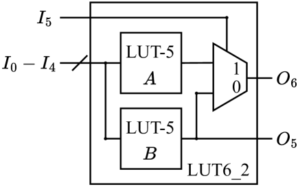
Figure 1: Architecture of dual-output LUTs in the UltraScale+ Series FPGA.

A LUT with $k$ inputs, denoted as LUT-$k$, can represent any Boolean function with $k$ inputs. In several modern FPGA architectures, two small LUTs can be merged into a dual-output LUT, which reduces the area of the design. For example, Fig. 1 shows the architecture of a dual-output LUT in the UltraScale+ Series FPGA [2]. The dual-output LUT-6, denoted as LUT6_2, is composed of two LUT-5s, $A$ and $B$, which share the same five inputs $I_{0},\ldots,I_{4}$. In Fig. 1, the output from LUT $B$ provides the first output $O_{5}$, while the second output $O_{6}$ is determined by an additional input $I_{5}$ that selects between the outputs of the two LUT-5s. Within the LUT6_2, the functions for LUT-5s $A$ and $B$ are denoted as $\mathcal{A}$ and $\mathcal{B}$, respectively.

III Methodology

In this section, we present the methodology of QUADOL and QUADOL+. First, we introduce the concept of approximately merging two single-output LUTs (i.e., a LUT pair) into one dual-output LUT in Section III-A. To reduce the error introduced by approximate LUT merging, Section III-B presents a method to automatically identify the optimal configuration for the dual-output LUT merged from a LUT pair, which determines the input signals and the functions for the dual-output LUT. To find as many mergable LUT pairs as possible for large area reduction, we propose to transform the problem of selecting multiple LUT pairs into a maximum matching problem for solving in Section III-C. Based on the above techniques, we finally present the entire flows of QUADOL and QUADOL+ in Sections III-D and III-E, respectively.

III-A Approximate LUT Merging

This section introduces the concept of approximate LUT merging. Traditional LUT merging involves combining two single-output LUTs into one with dual outputs. The constraints for exactly merging two LUTs are strict. For instance, if using the dual-output LUT architecture shown in Fig. 1, merging two distinct LUT-6s into a LUT6_2 is infeasible since the output $O_{5}$ can only express functions with up to five inputs. To further reduce the number of used LUTs, we propose approximate LUT merging. It allows approximately merging two single-output LUTs into a dual-output LUT, while only introducing a minimal error into the circuit.

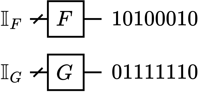
(a)

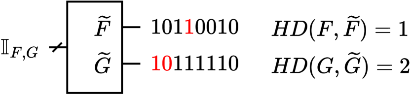
(b)

Figure 2: Approximately merging two single-output LUTs into one dual-output LUT: (a) before merging; (b) after merging.

Fig. 2 shows an example of approximately merging two single-output LUT-3s into a dual-output LUT. In what folllows, we denote the functions of the two single-output LUTs as $F$ and $G$, respectively. Their input signals are denoted as ${\color[rgb]{0,0,0}{\mathbb{I}}}_{F}$ and ${\color[rgb]{0,0,0}{\mathbb{I}}}_{G}$, respectively. Their exact truth tables are represented by the row vectors shown in Fig. 2(2(a)). For simplicity, in this paper, we use the term “merging functions $F$ and $G$” to mean merging their corresponding LUTs. After the approximate merging of these two LUTs, Fig. 2(2(b)) shows their approximate functions implemented by the dual-output LUT, which are denoted as $\widetilde{F}$ and $\widetilde{G}$, respectively. The input signals of the dual-output LUT is denoted as ${\color[rgb]{0,0,0}{\mathbb{I}}}_{F,G}$. The truth tables of $\widetilde{F}$ and $\widetilde{G}$ are shown as the row vectors in Fig. 2(2(b)), with the red entries in the vectors representing the flipped output values due to the approximation.

To measure the error for approximate LUT merging, first, we introduce the concept of Hamming Distance (HD). Specifically, the HD between an exact function $Y$ and its approximate function $\widetilde{{\color[rgb]{0,0,0}{Y}}}$, denoted as $\textit{HD}({\color[rgb]{0,0,0}{Y}},\widetilde{{\color[rgb]{0,0,0}{Y}}})$, is defined as the number of the input combinations where ${\color[rgb]{0,0,0}{Y}}$ and $\widetilde{{\color[rgb]{0,0,0}{Y}}}$ have different output values. For the example in Fig. 2(2(b)), $\textit{HD}(F,\widetilde{F})=1$ and $\textit{HD}(G,\widetilde{G})=2$. Then, we define the error $e$ brought by approximately merging $F$ and $G$ into a dual-output LUT as:

$$e=\textit{HD}(F,\widetilde{F})+\textit{HD}(G,\widetilde{G}).$$ (1)

Therefore, the objective is to minimize the error $e$. Thus, we need to determine the optimal configuration for the dual-output LUT merged from the functions $F$ and $G$. Specifically, we need to determine the input signals and the two output functions for the dual-output LUT.

III-B Configuring Dual-output LUT for Approximate Merging

This section proposes an approach to automatically determine the optimal configuration for the dual-output LUT. Most commercial FPGAs use LUT-6s as their fundamental LUT units [2, 3, 4, 5]. Once a circuit is mapped into such FPGAs, LUT-5s and LUT-6s occupy a large proportion of all mapped LUTs. By approximately merging LUT-5s and LUT-6s into dual-output LUTs, we can achieve substantial reduction in the number of LUTs. In this work, we focus on three types of LUT pairs that can be approximately merged: 1) two LUT-6s sharing six identical inputs; 2) two LUT-6s sharing five identical inputs; 3) one LUT-6 and one LUT-5 sharing five identical inputs. We call these three type of LUT pairs mergable LUT pairs. Moreover, we focus on the dual-output LUT architecture shown in Fig. 1. However, it is worth noting that our method can be adapted to other architectures with simple modifications. Next, we discuss how we approximately merge the three types of LUT pairs.

III-B1 Merging two LUT-6s sharing six identical inputs

Denote the identical inputs of $F$ and $G$ as $x_{0},x_{1},\ldots,x_{5}$. The configuration of LUT6_2 depends on the signals assigned to $I_{0},I_{1},\ldots,I_{5}$ and the assignment of $F$ and $G$ over the two outputs $O_{5}$ and $O_{6}$ of the LUT6_2. To minimize the error introduced by approximate LUT merging, we should keep as many original inputs as possible. Thus, five out of $x_{0},x_{1},\ldots,x_{5}$ should be assigned to $I_{0},I_{1},\dots,I_{4}$. The remaining input, $x_{i}$, is assigned to $I_{5}$ or not used. Therefore, $I_{5}$ is chosen from the set $\{1,x_{i},\overline{x_{i}}\}$, where $i\in\{0,1,\ldots,5\}$, and $I_{0},I_{1},\ldots,I_{4}$ are assigned with the other inputs signals. Note that since the truth table of a LUT can be arbitrarily modified, the signal $\overline{x_{i}}$ can be generated by negating the output of the LUT of $x_{i}$. In this case, for each LUT originally using $x_{i}$ as an input, to keep its global function, we can change its local function by replacing input $x_{i}$ with $\overline{x_{i}}$. Moreover, the constant 0 is not considered as a choice for $I_{5}$. This is because when the constant 0 is assigned to $I_{5}$, LUT-5 $A$ is not used, which has a larger error compared to the case where $I_{5}$ is assigned with constant $1$. For functions $F$ and $G$, they are derived from the set $\{O_{5},O_{6}\}$. Based on the above discussion, we list all configurations in Table I. Next, we will discuss how to derive the optimal functions for LUT-5s $A$ and $B$ for each configuration.

TABLE I: Configurations for LUT6_2 when merging two LUT-6s with six identical inputs.

$I_{5}$	$F$	$G$	LUT $A$	LUT $B$
$x_{i}$	$O_{6}$	$O_{5}$	$F_{x_{i}}$	$\textit{Maj}(F_{\overline{x_{i}}},G_{x_{i}},G_{\overline{x_{i}}})$
$x_{i}$	$O_{5}$	$O_{6}$	$G_{x_{i}}$	$\textit{Maj}(F_{x_{i}},F_{\overline{x_{i}}},G_{\overline{x_{i}}})$
$\overline{x_{i}}$	$O_{6}$	$O_{5}$	$F_{\overline{x_{i}}}$	$\textit{Maj}(F_{x_{i}},G_{x_{i}},G_{\overline{x_{i}}})$
$\overline{x_{i}}$	$O_{5}$	$O_{6}$	$G_{\overline{x_{i}}}$	$\textit{Maj}(F_{x_{i}},F_{\overline{x_{i}}},G_{x_{i}})$
$x_{i}$	$O_{6}$	$O_{6}$	$F_{x_{i}}$ or $G_{x_{i}}$	$F_{\overline{x_{i}}}$ or $G_{\overline{x_{i}}}$
$1$	$O_{6}$	$O_{5}$	$F_{x_{i}}$ or $F_{\overline{x_{i}}}$	$G_{x_{i}}$ or $G_{\overline{x_{i}}}$

The first row of Table I corresponds to the case where $F$ and $G$ are derived from $O_{6}$ and $O_{5}$ in LUT6_2, respectively, and $x_{i}$ is assigned to $I_{5}$. The approximate expressions for $F$ and $G$ can be written as $\widetilde{F}=x_{i}\mathcal{A}+\overline{x_{i}}\mathcal{B}$ and $\widetilde{G}=x_{i}\mathcal{B}+\overline{x_{i}}\mathcal{B}$, respectively, where $\mathcal{A}$ and $\mathcal{B}$ represent the functions for LUT-5s $A$ and $B$ in Fig. 1, respectively. Since $F=x_{i}F_{x_{i}}+\overline{x_{i}}F_{\overline{x_{i}}}$, where $F_{x_{i}}$ and $F_{\overline{x_{i}}}$ are the cofactors of $F$ when $x_{i}$ is true and false, respectively, $\textit{HD}(F,\widetilde{F})$ equals $\textit{HD}(\mathcal{A},F_{x_{i}})+\textit{HD}(\mathcal{B},F_{\overline{x_{i}}})$. Similarly, $\textit{HD}(G,\widetilde{G})=\textit{HD}(\mathcal{B},G_{x_{i}})+\textit{HD}(\mathcal{B},G_{\overline{x_{i}}})$. Therefore, $\textit{HD}(F,\widetilde{F})+\textit{HD}(G,\widetilde{G})$ equals $\textit{HD}(\mathcal{A},F_{x_{i}})+\textit{HD}(\mathcal{B},F_{\overline{x_{i}}})+\textit{HD}(\mathcal{B},G_{x_{i}})+\textit{HD}(\mathcal{B},G_{\overline{x_{i}}})$. To minimize the term $\textit{HD}(\mathcal{A},F_{x_{i}})$, $\mathcal{A}$ should be set to $F_{x_{i}}$. To minimize the remaining parts, $\mathcal{B}$ can be determined through the majority among $F_{\overline{x_{i}}}$, $G_{x_{i}}$ and $G_{\overline{x_{i}}}$, i.e., $B=\textit{Maj}(F_{\overline{x_{i}}},G_{x_{i}},G_{\overline{x_{i}}})$ [23].

The second row of Table I corresponds to the case where $G$ is derived from $O_{6}$ and $F$ from $O_{5}$, and $x_{i}$ is assigned to $I_{5}$. It is equivalent to swapping $F$ and $G$ in the first row. Therefore, $\mathcal{A}$ and $\mathcal{B}$ can be straightforwardly obtained by swapping $F$ and $G$ in the expressions for $\mathcal{A}$ and $\mathcal{B}$ in the first row.

The third and fourth rows of Table I represent the configuration of LUT6_2 when $\overline{x_{i}}$ is assigned to $I_{5}$. It is equivalent to swapping $x_{i}$ and $\overline{x_{i}}$ in the first and second rows. Therefore, $\mathcal{A}$ and $\mathcal{B}$ can be obtained by swapping $x_{i}$ and $\overline{x_{i}}$ in the expressions for $\mathcal{A}$ and $\mathcal{B}$ in the first and second rows.

When $x_{i}$ is assigned to $I_{5}$, there exists a special case where both $F$ and $G$ are derived from $O_{6}$. The fifth row of Table I corresponds to this case. In this case, $\textit{HD}(F,\widetilde{F})+\textit{HD}(G,\widetilde{G})$ equals $\textit{HD}(\mathcal{A},F_{x_{i}})+\textit{HD}(\mathcal{B},F_{\overline{x_{i}}})+\textit{HD}(\mathcal{A},G_{x_{i}})+\textit{HD}(\mathcal{B},G_{\overline{x_{i}}})$. Thus, $\mathcal{A}$ should be set to either $F_{x_{i}}$ or $G_{x_{i}}$, and $\mathcal{B}$ should be set to either $F_{\overline{x_{i}}}$ or $G_{\overline{x_{i}}}$. Note that both $\mathcal{A}$ and $\mathcal{B}$ have two potential choices, as they yield the same total HD. To determine the optimal choice, a simulation for each choice is performed, and the one causing the least error in the primary outputs is chosen. Note that we do not need to consider the case where $\overline{x_{i}}$ is assigned to $I_{5}$ and both $F$ and $G$ are derived from $O_{6}$. Its optimal solution can be derived by swapping the functions $\mathcal{A}$ and $\mathcal{B}$ in the optimal solution for the case where $x_{i}$ is assigned to $I_{5}$, and the optimal total HD is the same. Also, there is no need to consider the case where both $F$ and $G$ are derived from $O_{5}$, because in this case, LUT-5 $A$ is not used, causing more error than the case where both $F$ and $G$ are derived from $O_{6}$.

The sixth row of Table I presents another special case where the constant 1 is assigned to $I_{5}$. In this case, LUT6_2 operates as two separate LUT-5s, with one producing $F$ and the other producing $G$. Suppose that LUT $A$ produces $F$ and $B$ produces $G$. As a result, $F$ is derived from $O_{6}$, and $G$ from $O_{5}$. The total HD, $\textit{HD}(F,\widetilde{F})+\textit{HD}(G,\widetilde{G})$, equals $\textit{HD}(\mathcal{A},F_{x_{i}})+\textit{HD}(\mathcal{A},F_{\overline{x_{i}}})+\textit{HD}(\mathcal{B},G_{x_{i}})+\textit{HD}(\mathcal{B},G_{\overline{x_{i}}})$. Therefore, $\mathcal{A}$ should be either $F_{x_{i}}$ or $F_{\overline{x_{i}}}$, and $\mathcal{B}$ should be either $G_{x_{i}}$ or $G_{\overline{x_{i}}}$. Similar to the previous case, a simulation for each choice is performed, and the one with the least error in the primary outputs is chosen. Note that there is no need to consider the case where LUT $A$ produces $G$ and $B$ produces $F$, as the optimal total HD would remain the same.

In the approximate LUT merging method, the optimal total HD for each row in Table I is calculated. The configuration with the smallest total HD is selected as the optimal configuration for $x_{i}$. Given that $F$ and $G$ share six identical inputs, we perform the above procedure for each $x_{i}$ from the set $\{x_{0},x_{1},\ldots,x_{5}\}$. Among these choices, we select the one with the smallest total HD as the optimal configuration for merging $F$ and $G$. Moreover, when performing approximate LUT merging on $F$ and $G$, the negations of $F$ and $G$ are also considered. This means that the optimal configuration is identified not only for $F$ and $G$, but also for $\overline{F}$ and $G$, as well as $F$ and $\overline{G}$. Note that there is no need to consider the pair $\overline{F}$ and $\overline{G}$, since the optimal configuration for the pair can be obtained by negating $\mathcal{A}$ and $\mathcal{B}$ in the optimal configuration for merging $F$ and $G$, yielding the same total HD. Among these three pairs (i.e., $F$ and $G$, $\overline{F}$ and $G$, and $F$ and $\overline{G}$), the one with the least HD is selected. If $\overline{F}$ (resp. $\overline{G}$) is produced after approximate LUT merging, an input negation is performed on the LUTs with $F$ (resp. $G$) as an input to restore their functions.

III-B2 Merging two LUT-6s sharing five identical inputs

The process of merging two single-output LUT-6s with five identical inputs into one LUT6_2 is similar to merging two LUT-6s with six identical inputs. The major difference arises from the unique input signals of $F$ and $G$. Denote the shared inputs of $F$ and $G$ as $x_{0},x_{1},\ldots,x_{4}$ and the unique inputs of $F$ and $G$ as $m$ and $n$, respectively. Thus, function $F$ is independent of $n$ and $G$ is independent of $m$. In the structure of LUT6_2, $O_{6}$ depends on $I_{0},I_{1},\ldots,I_{5}$, while $O_{5}$ depends on $I_{0},I_{1},\ldots,I_{4}$. Regardless of whether $F$ and $G$ are assigned to $O_{5}$ or $O_{6}$, to minimize the error in the approximate merging, a good choice is to assign the shared inputs of $F$ and $G$, $x_{0},x_{1},\ldots,x_{4}$, to $I_{0},I_{1},\ldots,I_{4}$. Similar to merging two LUT-6s with six idential inputs, the remaining input, $I_{5}$, should be chosen from the set $\{1,m,\overline{m},n,\overline{n}\}$. Table II lists all configuration for the LUT6_2.

The first row lists the configuration of LUT6_2 when $m$ is assigned to $I_{5}$. Since $O_{5}$ is independent of $I_{5}$ and $G$ is independent of $m$, it is more appropriate to derive $G$ from $O_{5}$ rather than $O_{6}$. Accordingly, $F$ should be derived from $O_{6}$. The approximate expressions for $F$ and $G$ become $\widetilde{F}=m\mathcal{A}+\overline{m}\mathcal{B}$ and $\widetilde{G}=n\mathcal{B}+\overline{n}\mathcal{B}$, respectively. The total HD, $\textit{HD}(F,\widetilde{F})+\textit{HD}(G,\widetilde{G})$, becomes $\textit{HD}(\mathcal{A},F_{m})+\textit{HD}(\mathcal{B},F_{\overline{m}})+\textit{HD}(\mathcal{B},G_{n})+\textit{HD}(\mathcal{B},G_{\overline{n}})$. To minimize it, $\mathcal{A}$ should be set as $F_{m}$, and $\mathcal{B}$ should be set as $\textit{Maj}(F_{\overline{m}},G_{n},G_{\overline{n}})$.

The second row in Table II represents the configuration of LUT6_2 when $n$ is assigned to $I_{5}$. It is equivalent to swapping $m$ and $n$ in the first row. Accordingly, $F$ and $G$ should also be swapped. The functions $\mathcal{A}$ and $\mathcal{B}$ can be determined by swapping $F$ and $G$ as well as $m$ and $n$ in the expressions for $\mathcal{A}$ and $\mathcal{B}$ in the first row.

The third and fourth rows in Table II give the configuration of LUT6_2 when $\overline{m}$ and $\overline{n}$ are assigned to $I_{5}$, respectively. The third (resp., fourth) row is equivalent to swapping $m$ and $\overline{m}$ (resp., $n$ and $\overline{n}$) in the first (resp., second) row. Therefore, $\mathcal{A}$ and $\mathcal{B}$ can also be obtained correspondingly.

The fifth row in Table II presents the configuration of LUT6_2 when the constant $1$ is assigned to $I_{5}$. In this case, LUT6_2 operates as two separate LUT-5s, with one producing $F$ and the other producing $G$. Suppose that LUT $A$ produces $F$ and $B$ produces $G$. $\mathcal{A}$ and $\mathcal{B}$ for this case can be obtained in a similar way as merging two LUT-6s with six identical inputs.

TABLE II: Configurations for LUT6_2 when merging two LUT-6s with five identical inputs.

$I_{5}$	$F$	$G$	LUT $A$	LUT $B$
$m$	$O_{6}$	$O_{5}$	$F_{m}$	$\textit{Maj}(F_{\overline{m}},G_{n},G_{\overline{n}})$
$n$	$O_{5}$	$O_{6}$	$G_{n}$	$\textit{Maj}(F_{m},F_{\overline{m}},G_{\overline{n}})$
$\overline{m}$	$O_{6}$	$O_{5}$	$F_{\overline{m}}$	$\textit{Maj}(F_{m},G_{n},G_{\overline{n}})$
$\overline{n}$	$O_{5}$	$O_{6}$	$G_{\overline{n}}$	$\textit{Maj}(F_{m},F_{\overline{m}},G_{n})$
$1$	$O_{6}$	$O_{5}$	$F_{m}$ or $F_{\overline{m}}$	$G_{n}$ or $G_{\overline{n}}$

III-B3 Merging one LUT-6 and one LUT-5 sharing five identical inputs

Assume $F$ is the function for the LUT-6 and $G$ is the function for the LUT-5. Denote the identical inputs for $F$ and $G$ as $x_{0},x_{1},\ldots,x_{4}$ and the unique input for $F$ as $m$. Thus, function $G$ is independent of $m$. Same as merging two LUT-6s with five identical inputs, the shared inputs of $F$ and $G$, $x_{0},x_{1},\ldots,x_{4}$, should be assigned to $I_{0},I_{1},\ldots,I_{4}$. The difference is that $I_{5}$ should be selected from the set $\{1,m,\overline{m}\}$. Table III lists all configuration for the LUT6_2.

The first row in Table III lists the configuration of LUT6_2 when $m$ is assigned to $I_{5}$. In this case, $O_{6}$ and $F$ have the same set of inputs, and so do $O_{5}$ and $G$. Thus, $F$ and $G$ should be derived from $O_{6}$ and $O_{5}$, respectively. The approximate expressions for $F$ and $G$ become $\widetilde{F}=m\mathcal{A}+\overline{m}\mathcal{B}$ and $\widetilde{G}=\mathcal{B}$. The total HD, $\textit{HD}(F,\widetilde{F})+\textit{HD}(G,\widetilde{G})$, equals $\textit{HD}(\mathcal{A},F_{m})+\textit{HD}(\mathcal{B},F_{\overline{m}})+\textit{HD}(\mathcal{B},G)$. To minimize it, $\mathcal{A}$ should be set to $F_{m}$ and $\mathcal{B}$ should be set to either $F_{\overline{m}}$ or $G$.

The second row in Table III gives the configuration of LUT6_2 when $\overline{m}$ is assigned to $I_{5}$. It is equivalent to swapping $m$ and $\overline{m}$ in the first row. Therefore, $\mathcal{A}$ and $\mathcal{B}$ can be obtained correspondingly.

The third row of Table III represents the configuration of LUT6_2 when the constant 1 is assigned to $I_{5}$. In this case, LUT6_2 operates as two separate LUT-5s, with one producing $F$ and the other producing $G$. Suppose that LUT $A$ produces $F$ and $B$ produces $G$. As a result, $\textit{HD}(F,\widetilde{F})+\textit{HD}(G,\widetilde{G})$ equals $\textit{HD}(\mathcal{A},F_{m})+\textit{HD}(\mathcal{A},F_{\overline{m}})+\textit{HD}(\mathcal{B},G)$. To minimize it, $\mathcal{A}$ should be either $F_{m}$ or $F_{\overline{m}}$ and $\mathcal{B}$ should be $G$.

TABLE III: Configurations for LUT6_2 when merging two LUT-6s with 5 same inputs.

$I_{5}$	$F$	$G$	LUT $A$	LUT $B$
$m$	$O_{6}$	$O_{5}$	$F_{m}$	$F_{\overline{m}}$ or $G$
$\overline{m}$	$O_{6}$	$O_{5}$	$F_{\overline{m}}$	$F_{m}$ or $G$
1	$O_{6}$	$O_{5}$	$F_{m}$ or $F_{\overline{m}}$	$G$

III-C Selecting Multiple LUT Pairs

To reduce the number of LUTs used in the final design, this section aims to merge as many LUT pairs as possible. However, there may exist conflicts among different LUT pairs, preventing them from being merged. As shown in Fig. 3, while LUTs $F$ and $G$ can be merged, and LUTs $G$ and $K$ can also be merged, these merging processes cannot occur concurrently. This is because the signal $G$ can only be driven once. Simultaneously merging these two LUT pairs would result in a multi-driven issue. Therefore, when two LUT pairs share the same LUT member, they are in conflict and cannot be merged simultaneously. To maximize the area reduction in the final design, we aim to merge as many non-conflicting LUT pairs as possible among the candidate LUT pairs. To address this, a graph is constructed where each node represents a LUT, and an edge between two nodes means that the two LUTs corresponding to the two nodes can be approximately merged. Fig. 4(4(a)) shows an example of such a graph with 6 candidate LUTs. Our goal is to identify the maximum number of edges that do not connect with each other in the graph. This is a maximum matching problem on graph and can be solved by a maximum matching algorithm [24]. After identifying the maximum matching in the graph, all LUT pairs corresponding to the found edges are merged simultaneously to form the approximate circuit. For example, as shown in Fig. 4(4(a)), the three LUT pairs denoted as the edges marked with red circles (i.e., LUTs $L_{1}$ and $L_{2}$, $L_{3}$ and $L_{4}$, and $L_{5}$ and $L_{6}$) can be merged simultaneously.

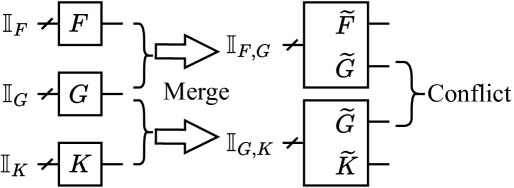
Figure 3: A sample of conflicting LUT pairs.

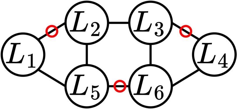
(a)

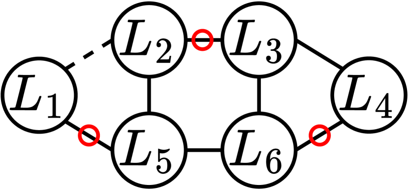
(b)

Figure 4: Two different maximum matching solutions.

Given a graph, there may exist multiple maximum matching solutions. For example, the two sets of edges marked with red circles in Figs. 4(4(a)) and (4(b)) give two distinct maximum matching solutions for the same graph. However, it is hard to obtain the exact number of maximum matching solutions for a given graph. To address this, we propose a randomized method to find $k$ different maximum matching solutions for each graph, where $k$ is a given number from user, and stands for the expected number of solutions. Specifically, once a new maximum matching solution is found, one of its LUT pairs is randomly chosen and omitted in the search for next solution. For example, the dashline in Fig. 4(4(b)) means that the LUT pair $(L_{1},L_{2})$ has been randomly chosen and omitted after the solution in Fig. 4(4(a)) is found. This ensures that the new solution in Fig. 4(4(b)) is different from the initial solution in Fig. 4(4(a)).

III-D Flow of QUADOL

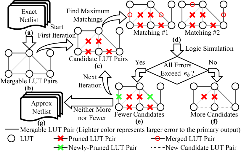
Figure 5: The overall flow of QUADOL.

This sections presents the entire flow of QUADOL, which is based on the approximate dual-output LUT configuration method presented in Section III-B and the LUT pair selection method presented in Section III-C. Fig. 5 illustrates the overall flow of QUADOL. It exploits the idea of binary search to speed up the process. Initially, QUADOL identifies all mergable LUT pairs in the given exact netlist (see Fig. 5(a)). The edges in Fig. 5(b) represent these LUT pairs from the given exact netlist. However, some of them may induce substantial errors after approximate LUT merging, which should be pruned prior to the search for optimal LUT pairs. Thus, for each LUT pair, QUADOL evaluates its error at the primary output through logic simulation. Note that in Fig. 5, the edges with lighter colors represent LUT pairs with larger errors.

After evaluating the errors, QUADOL starts an iterative process, which corresponds to Figs. 5(c)–(f). In the first iteration, half of the LUT pairs with the largest errors are pruned. For example, the LUT pairs corresponding to the edges marked with a red cross in Fig. 5(c) are pruned. The remaining LUT pairs are referred to as candidate LUT pairs. The next step of QUADOL, which is shown in Fig. 5(d), searches for $k$ maximum matching solutions, where $k=2$ in this example. For each solution, all matched LUT pairs are merged, resulting in $k$ approximate circuits. QUADOL then performs logic simulation on the obtained circuits to get their errors. If the errors of all circuits exceed a given error bound $e_{b}$, half of the current candidate LUT pairs are further pruned. For example, in Fig. 5(d), there are four candidate LUT pairs. Then, as shown in Fig. 5(e), half of them are further pruned for the next iteration, which are indicated by two edges with a green cross. In contrast, if there exists a circuit whose error is within $e_{b}$, half of the pruned LUT pairs are reconsidered as the candidate LUT pairs in the next iteration. For example, there are four pruned LUT pairs in Fig. 5(d). Half of them are reverted to candidate LUT pairs for the next iteration, as shown in Fig. 5(f), where the two edges in dashed line indicate the reconsidered candidate LUT pairs. This process, which basically borrows the idea of binary search, continues until the candidate LUT pairs can neither be increased nor decreased. Finally, QUADOL selects the maximum matching over the current candidate LUT pairs that has the least error at the primary outputs among all $k$ randomly constructed maximum matchings as the final output (see Fig. 5(g)).

III-E Flow of QUADOL+

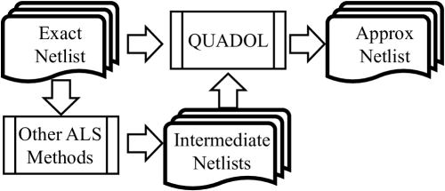
Figure 6: The overall flow of QUADOL+.

Since QUADOL proposed in Section III-D exploits a new dimensions, i.e., approximately merging a LUT pair into a dual-output LUT, which is never exploited by the previous ALS methods, it can be integrated with any existing ALS methods to strengthen them. Thus, we also introduce QUADOL+, which is a generic framework to integrate QUADOL into existing ALS methods. Its overall flow is shown in Fig. 6. Given an exact netlist and several other ALS methods, these ALS methods are first applied to the exact netlist. In this process, these methods would generate many intermediate approximate netlists. After that, QUADOL takes the exact netlist and the intermediate netlists as its inputs and further optimize the intermediate netlists, where the exact one is used as a reference circuit for error measurement purpose. Finally, the best result optimized by QUADOL is taken as the final optimal result for QUADOL+.

IV Experimental Results

This section presents the experimental results. We conduct all experiments on a 64-core AMD Threadripper PRO 5995WX processor running at 2.7GHz with 512GB RAM and use 32 cores for our experiments. We employ error rate (ER) and mean relative error distance (MRED) as the error metrics. ER is the probability of error, and MRED measures the average relative error distance as follows:

$$\textit{MRED}=\sum^{2^{I}}_{i=1}\frac{\left|\hat{y_{i}}-y_{i}\right|\cdot p_{i}}{\text{max}\left\{y_{i},1\right\}},\vspace{-0.1cm}$$ (2)

where $I$ is the number of primary inputs, $\hat{y_{i}}$ and $y_{i}$ are the approximate and accurate output values, respectively, for the $i$-th input combination, and $p_{i}$ is the probability of the $i$-th input combination. The denominator in Eq. (2) is set as the maximum between the accurate output value $y_{i}$ and 1 to avoid division by zero. In our experiments, the input combinations for each circuit are uniformly distributed.

The area ratio, defined as the number of LUTs in the approximate circuit relative to the exact one, is used to evaluate the area performance of the approximated designs. Smaller area ratios are favored. To assess the area ratio improvement of our methods over the baseline method, we use relative area ratio, which is the average area ratio of our methods over that of the baseline method.

The number of maximum matching solutions per iteration, denoted as $k$, is set to 16. This is due to the fact that identifying the maximum matching for a graph is an NP-hard problem and can be time-consuming. Seeking more solutions could result in extended runtime, while seeking fewer solutions might overlook those with smaller errors. We find that searching for at most 16 solutions achieves a good trade-off between runtime and quality.

IV-A Comparison with Other ALS Methods

In this section, we study the performances of QUADOL and QUADOL+. We compare them with two state-of-the-art ALS methods for FPGA, ALSRAC [17] and Xiang’s method [18]. Here, QUADOL+ is built by integrating QUADOL with ALSRAC [17] and Xiang’s method [18] together. Furthermore, the intermediate approximate netlists used in QUADOL+ are produced by running ALSRAC and Xiang’s method 10 times and then selecting the best results. All these best results are also used to represent ALSRAC and Xiang’s method in the comparison.

EPFL benchmark [21] and IWLS benchmark [22] are used to evaluate the performance of QUADOL+. Table IV lists the benchmark circuits used in our experiments, along with their LUT numbers after mapping to LUT-6. For circuits in AIG representations, they are fully optimized and mapped to LUT-6 by ABC [25] using the script “$\textit{sweep};\textit{strash};\textit{resyn2}\times 10;\textit{if -K 6};$” to ensure that these circuits cannot be further optimized by traditional logic synthesis. Note that we ignore the small circuits and only focus on the large ones since they are more challenging.

TABLE IV: Benchmarks used in our experiments.

IWLS Benchmark				EPFL Arithmetic
Circuit	LUT Num	Circuit	Size	Circuit	LUT Num
apex1	490	rd84	131	divisor	3267
apex3	527	rot	188	log2	6567
apex4	799	seq	883	multiplier	4919
cps	434	table3	333	sine	1227
dalu	228	table5	291	sqrt	3074
des	1104	vda	237	square	3241
ex5p	526

IV-A1 Comparison under ER constraint

IWLS circuits are used as the benchmark under 2 ER thresholds, 1% and 2%, and the final result for each circuit is the average result over these two ER thresholds. Fig. 7 shows the relative area ratio for the results from Xiang’s method [18], ALSRAC [17], and QUADOL+, where the results of Xiang’s method [18] are taken as the baseline. he numbers on the figure represent the values of relative area ratios for QUADOL+. On average, QUADOL+ improves the relative area ratio by $18.15\%$ and $2.39\%$ over Xiang’s method and ALSRAC, respectively. However, QUADOL+ is $1.75\times$ slower than Xiang’s method, and $3.50\times$ slower than ALSRAC. This is because it has to wait for the intermediate netlists from them for further optimization.

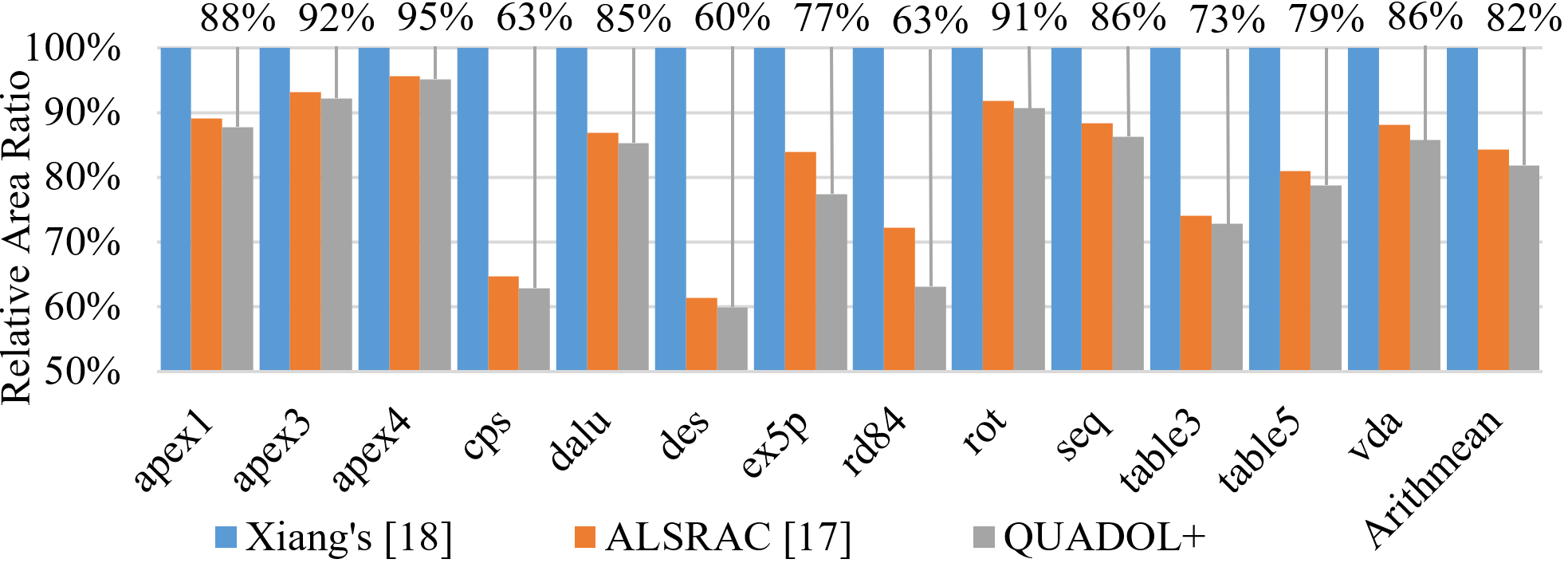
Figure 7: Relative area ratio for Xiang’s method [18], ALSRAC [17], and QUADOL+ under ER constraint.

IV-A2 Comparison under MRED constraint

We also compare QUADOL, QUADOL+, and ALSRAC [17] on EPFL circuits under three MRED thresholds: 0.05%, 0.1%, and 0.5%, and the final result for each circuit is the average result over these three MRED thresholds. Since Xiang’s method [18] cannot handle the MRED metric, it is not included in the comparison. Therefore, only ALSRAC is compared. Fig. 8 shows the relative area ratio of QUADOL and QUADOL+ with ALSRAC as the baseline. The numbers on the figure represent the values of relative area ratios for QUADOL and QUADOL+. As shown in the figure, QUADOL cannot beat ALSRAC. This is because ALSRAC considers all signals in the technology independent representation of a circuit as the optimization candidates, offering more opportunities for improvement than QUADOL, which only focuses on LUTs in a synthesized FPGA design. However, the combination of QUADOL and ALSRAC, i.e., QUADOL+, outperforms ALSRAC, since QUADOL can strengthen ALSRAC by exploiting dual-output LUTs in modern FPGA. On average, QUADOL+ improves ALSRAC’s area ratio by 12.16%. QUADOL+ shows a significant improvement on the div circuit, where ALSRAC only achieve 5% area ratio decrease on the original circuit. In contrast, QUADOL+ improves ALSRAC’s results by 22.85%. However, QUADOL+ shows less than 1% improvement on the sqrt circuit. This is because ALSRAC reduce the area ratio of the original circuit by 97%, and further optimization on it is hard. In that case, QUADOL+ still finds and merges 1 LUT pair within the error threshold based on the result from ALSRAC, and further decreases the area ratio.

In terms of delay, neither QUADOL nor QUADOL+ can reduce the delay of a circuit, as approximate LUT merging does not reduce the number of LUTs on the critical path. For this reason, compared to ALSRAC, our methods do not improve the delay. However, it is also important to note that they would not worsen the delay either. This is because the outputs of the merged LUTs only depend on their inputs before merging, not on any other signals. Therefore, approximate LUT merging does not increase the number of LUTs on the critical path.

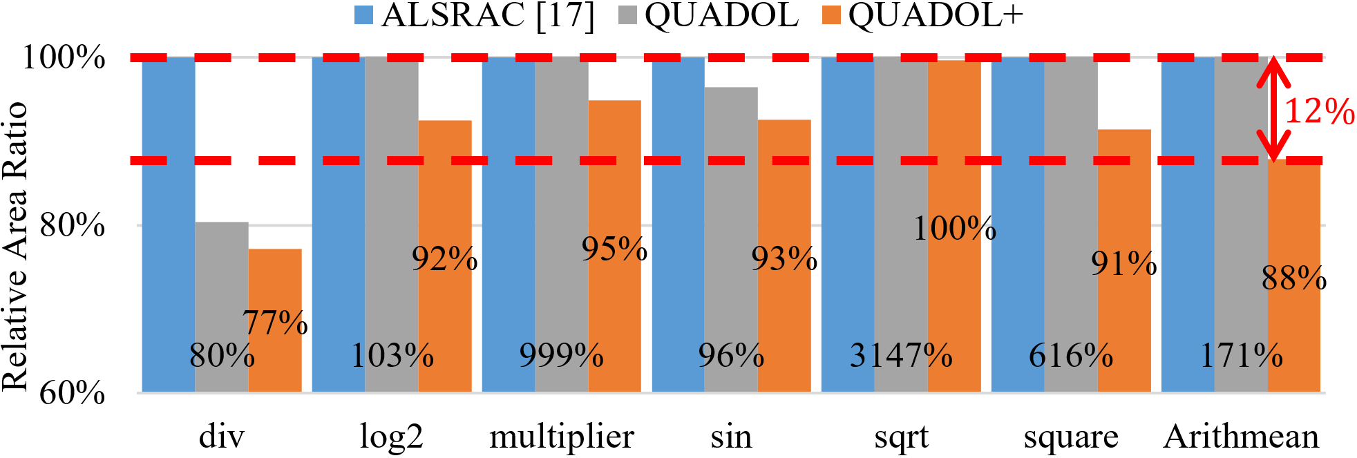
Figure 8: Relative area ratio for ALSRAC [17], QUADOL and QUADOL+ under MRED constraints.

IV-B Comparison with Other FPGA-based Approximate Multipliers

In this section, we study the performances of QUADOL+ on FPGA-based approximate multipliers. We take approximate multipliers from EAL [26] as the intermediate netlists in QUADOL+ and compare the obtained results with approximate multipliers from EAL [26], LM [12], SMA [9], Ca [14], and Guo [13]. Since multipliers from EAL [26] are in RTL format, we synthesize them into netlists by ABC, and use the script “$\textit{sweep};\textit{strash};\textit{resyn2}\times 10;\textit{if -K 6};$” to optimize these circuits. [13] provides a comprehensive measurement for multipliers in LM [12], SMA [9], Ca [14], and Guo [13]. We directly use the LUT numbers and MRED measured in [13]. For a fair comparison, the CARRY4 [27] usage is not taken into consideration. We also synthesize the multipliers generated by QUADOL+ on Vivado 2022.2 [28] for FPGA component xc7vx485tffg1157-1. DSP blocks and CARRY4 units are disable when synthesizing the results from QUADOL+. We set the error bound $e_{b}$ for QUADOL+ as 100%, and record all netlists generated in the experiment. Then, we do logic synthesis and simulation on the netlists generated by QUADOL+. Based on the synthesis and simulation results, we obtain several Pareto fronts in the area-error plane for QUADOL+, with each Pareto front representing one type of multipliers.

Figs. 9(9(a)) and (9(b)) show the comparison between other FPGA-based approximate multipliers and results from QUADOL+ on 8-bit multipliers and 16-bit multipliers under MRED constraint. As shown, the results from QUADOL+ dominate most of the previous proposed multipliers without using CARRY4 units or DSP blocks on FPGA. Through our detailed analysis, we find it is because 8-bit and 16-bit multipliers in [12, 14, 13] are built up from hand-crafted 4-bit multipliers. They overlook the optimization space between 4-bit multipliers. In contrast, QUADOL+ can recognize mergable LUT pairs between these 4-bit multipliers and merge them together.

(a) 8-bit multiplier.

(b) 16-bit multiplier.

Figure 9: Comparison between other FPGA-based approximate multipliers and QUADOL+’s results under MRED constraint.

We also use QUADOL+ to generate approximate multipliers under ER constraint. Since multipliers in [12, 9, 14, 13] does not take ER into consideration, we only compare our results with EAL [26]. Figs. 9(9(a)) and (9(b)) show the comparison between EAL and QUADOL+ on four multipliers under ER constraint: 1) 7-bit multiplier; 2) 8-bit multiplier; 3) $8\times 2$ multiplier; and 4) $8\times 3$ multiplier. As shown, QUADOL+ cannot dominate all results from EAL. Nevertheless, it works well for very small ER constraints compared to EAL. When the ER constraint is large, most of the primary outputs are set to constant numbers or wires from other primary outputs. In that case, few LUTs can be approximately merged, reducing QUADOL+’s effectiveness.

(a) 7-bit and 8-bit multipliers.

(b) $8\times 2$ and $8\times 3$ multipliers.

Figure 10: Comparison between EAL [26] and QUADOL+ under ER constraint.

V Conclusion

This paper proposes QUADOL, a quality-driven ALS method that uses approximate LUT merging to minimize the number of LUTs required in FPGA designs. The main idea is to approximately merge two single-output LUTs into a dual-output LUT. We transform the problem of selecting multiple LUT pairs into a maximum matching problem to merge as many LUT pairs as possible. We propose a binary search-based ALS method for approximate LUT merging to accelerate the searching process. Since QUADOL exploits a new dimension, i.e., approximately merging a LUT pair into a dual-output LUT, it can be integrated with any existing ALS methods to strengthen them. Therefore, we also introduce QUADOL+, which is a generic framework to integrate QUADOL into existing ALS methods. The experimental results showed that QUADOL+ can reduce the LUT count by 18% compared to the state-of-the-art methods for FPGA. Moreover, the approximate multipliers optimized by QUADOL+ dominate most prior FPGA-based approximate multipliers in the area-error plane. In the future, we plan to support other dual-output LUT architectures, such as dual-output LUTs from Intel [5]. Moreover, we plan to further speed up the searching process for optimal LUT pairs.

References

- [1] M. Ahmadinejad et al., “Energy- and quality-efficient approximate multipliers for neural network and image processing applications,” TETC, vol. 10, no. 2, pp. 1105–1116, 2022.
- [2] Xilinx, “LUT6_2,” in UltraScale Architecture Libraries Guide. AMD, Inc., 2024, ch. 5, pp. 437–441.
- [3] B. Gaide et al., “Xilinx adaptive compute acceleration platform: Versal™ architecture,” in FPGA, 2019, pp. 84–93.
- [4] J. Chromczak et al., “Architectural enhancements in Intel® Agilex™ FPGAs,” in FPGA, 2020, pp. 140–149.
- [5] Intel, “Adaptive Logic Module,” in Intel® Arria® 10 Device Overview. Intel, Inc., 2018, pp. 17–18.
- [6] F. Wang et al., “Dual-output LUT merging during FPGA technology mapping,” in ICCAD, 2020, pp. 1–9.
- [7] B. S. Prabakaran et al., “DeMAS: An efficient design methodology for building approximate adders for FPGA-based systems,” in DATE, 2018, pp. 917–920.
- [8] S. Ullah et al., “Area-optimized low-latency approximate multipliers for FPGA-based hardware accelerators,” in DAC, 2018, pp. 1–6.
- [9] ——, “SMApproxLib: Library of FPGA-based approximate multipliers,” in DAC, 2018, pp. 1–6.
- [10] Y. Guo et al., “Small-area and low-power FPGA-based multipliers using approximate elementary modules,” in ASP-DAC, 2020, pp. 599–604.
- [11] S. Yao and L. Zhang, “FHAM: FPGA-based high-efficiency approximate multipliers via LUT encoding,” in ICCD, 2022, pp. 487–490.
- [12] ——, “Hardware-efficient FPGA-based approximate multipliers for error-tolerant computing,” in ICFPT, 2022, pp. 1–8.
- [13] Y. Guo et al., “Hardware-efficient multipliers with FPGA-based approximation for error-resilient applications,” TCAS, pp. 1–12, 2024.
- [14] S. Ullah et al., “High-performance accurate and approximate multipliers for FPGA-based hardware accelerators,” TCAD, vol. 41, no. 2, pp. 211–224, 2022.
- [15] Y. Wu et al., “Approximate logic synthesis for FPGA by wire removal and local function change,” in ASP-DAC, 2017, pp. 163–169.
- [16] B. S. Prabakaran et al., “ApproxFPGAs: Embracing ASIC-based approximate arithmetic components for FPGA-based systems,” in DAC, 2020, pp. 1–6.
- [17] C. Meng et al., “ALSRAC: Approximate logic synthesis by resubstitution with approximate care set,” in DAC, 2020, pp. 1–6.
- [18] Z. Xiang et al., “Approximate logic synthesis for FPGA by decomposition,” in Approximate Computing, W. Liu and F. Lombardi, Eds. Springer, 2022, ch. 7, pp. 149–174.
- [19] M. Barbareschi et al., “FPGA approximate logic synthesis through catalog-based AIG-rewriting technique,” JSA, vol. 150, p. 103112, 2024.
- [20] I. Scarabottolo et al., “Approximate logic synthesis: A survey,” Proc. IEEE, vol. 108, no. 12, pp. 2195–2213, 2020.
- [21] EPFL, “The EPFL combinational benchmark suite,” https://www.epfl.ch/labs/lsi/page-102566-en-html/benchmarks/, 2023.
- [22] IWLS, “IWLS 2005 benchmarks,” https://iwls.org/iwls2005/benchmarks.html, 2005.
- [23] J. Chen et al., “On computing centroids according to the -norms of Hamming distance vectors,” in ESA, vol. 144, 2019, pp. 28:1–28:16.
- [24] Z. Galil, “Efficient algorithms for finding maximum matching in graphs,” ACM Comput. Surv., vol. 18, no. 1, pp. 23––38, March 1986.
- [25] A. Mishchenko et al., “ABC: a system for sequential synthesis and verification, release 90703,” http://people.eecs.berkeley.edu/~alanmi/abc/, accessed July 3, 2019.
- [26] V. Mrazek et al., “EvoApproxLib: Extended library of approximate arithmetic circuits,” in WOSET, 2019, p. 10.
- [27] Xilinx, “CARRY4,” in Vivado Design Suite 7 Series FPGA and Zynq 7000 SoC Libraries Guide. AMD, Inc., 2024, ch. 5, pp. 302–304.
- [28] ——, in Vivado Design Suite User Guide. AMD, Inc., 2024.