SRG Analysis of Lur’e Systems and the Generalized Circle Criterion

Abstract

Scaled Relative Graphs (SRGs) provide a novel graphical frequency-domain method for the analysis of nonlinear systems. However, we show that the current SRG analysis suffers from some pitfalls that limit its applicability in analysing practical nonlinear systems. We overcome these pitfalls by modifying the SRG of a linear time invariant operator, combining the SRG with the Nyquist criterion, and apply our result to Lur’e systems. We thereby obtain a generalization of the celebrated circle criterion, which deals with broader class of nonlinearities, and provides (incremental) $L^{2}$-gain performance bounds. We illustrate the power of the new approach on the analysis of the controlled Duffing oscillator.

I Introduction

In the case of a Linear Time Invariant (LTI) system, graphical system analysis using the Nyquist diagram [1] is the cornerstone of control engineering. It is easy to use, and allows for intuitive analysis and controller design methods. However, it is unclear how to generalize graphical frequency domain methods to nonlinear system analysis and controller design.

There have been various attempts in extending graphical analysis methods for nonlinear systems, but they are all either approximate, or limited in range of applicability. Classical results such as the circle criterion [2], which is based on the Nyquist concept, and the Popov criterion can predict the stability of a class of nonlinear systems. These methods are exact, but are not useful for performance shaping. Moreover, they are limited to Lur’e systems with sector bounded nonlinearities. The describing function method [3] is an approximate method based on the Nyquist diagram, which considers only the first Fourier coefficient of the amplitude-dependent frequency response. A more sophisticated approximate method is the nonlinear bode diagram in [4]. The Scaled Relative Graph (SRG) [5] proposed in [6] is a new graphical method to analyze nonlinear feedback systems. It is an exact method, and it is intuitive because of its close connection to the Nyquist diagram. Moreover, SRG analysis can provide performance bounds in terms of (incremental) $L^{2}$-gain. This has been demonstrated recently in [7], where the framework of SRGs has been applied to the analysis of reset controllers.

Even though existing SRG tools are exact they are limited in range of applicability, as they can only deal with stable open-loop plants. In practice, however, it is often required to stabilize an unstable nonlinear plant. In this paper, we demonstrate a fundamental pitfall of SRG analysis when applying it to handle unstable LTI systems in a feedback interconnection. We resolve this pitfall by including the information provided by the Nyquist criterion into the SRG of the LTI operator to obtain an effective tool for computing stability conditions. We then apply our solution to the Lur’e setup, for which we obtain performance metrics in terms of (incremental) $L^{2}$-gain bounds, and well-posedness is guaranteed via the homotopy construction [8]. An important consequence of our results is a generalized circle criterion, where the class of nonlinear operators is now general, instead of being limited to sector bounded nonlinearities as in the current sate-of-the-art results.

This paper is structured as follows. In Section II, we present the required preliminaries, and in Section III the SRG concept of nonlinear system analysis. An important pitfall of the current SRG methods is identified in Section IV, and its resolution is given in Section V, which implies a rather general extension of the celebrated circle criterion. We apply our main result to the example of disturbance rejection analysis for the Duffing oscillator in Section VI and present our conclusions in Section VII.

II Preliminaries

II-A Notation and Conventions

Let $\mathbb{R},\mathbb{C}$ denote the real and complex number fields, respectively, with $\mathbb{R}_{>0}=(0,\infty)$ and $\mathbb{C}_{\real>0}=\{a+jb\mid\,a\in\mathbb{R}_{>0},\,b\in\mathbb{R}\}$, where $j$ is the imaginary unit. We denote the complex conjugate of $z=a+jb\in\mathbb{C}$ as $\bar{z}=a-jb$. Let $\mathcal{L}$ denote a Hilbert space, with inner product $\innerproduct{\cdot}{\cdot}_{\mathcal{L}}:\mathcal{L}\times\mathcal{L}\to\mathbb{C}$ and norm $\norm{x}_{\mathcal{L}}:=\sqrt{\innerproduct{x}{x}_{\mathcal{L}}}$. For sets $A,B\subset\mathbb{C}$, the sum and product sets are defined as $A+B:=\{a+b\mid a\in A,b\in B\}$ and $AB:=\{ab\mid a\in A,b\in B\}$, respectively. The disk in the complex plane is denoted $D_{r}(x)=\{z\in\mathbb{C}\mid|z-x|\leq r\}$. Denote $D_{[\alpha,\beta]}$ the disk in $\mathbb{C}$ centered on $\mathbb{R}$ which intersects $\mathbb{R}$ in $[\alpha,\beta]$.

II-B Signals, Systems and Stability

A relation $R$ on a Hilbert space is a possibly multi-valued map $R:\mathcal{L}\to\mathcal{L}$. The graph of such a relation is the set $\{u,y\in\mathcal{L}\mid u\in\text{dom}(R),y\in R(u)\}$.

Given a relation $R$ on a normed space $\mathcal{L}$, the induced norm of the operator is defined as

$$\norm{R}_{\mathcal{L}}:=\sup_{u_{1},u_{2}\in\mathcal{L}}\frac{\norm{R(u_{1})-R(u_{2})}}{\norm{u_{1}-u_{2}}},$$ (1)

where $\norm{\cdot}$ denotes the norm of the space.

Denote a field $\mathbb{F}\in\{\mathbb{R}^{d},\mathbb{C}^{d}\}$, where $d=1$ is assumed, unless specified otherwise, since this work focuses on SISO continuous time systems. One Hilbert space of particular interest is $L^{2}(\mathbb{F}):=\{f:\mathbb{R}_{\geq 0}\to\mathbb{F}\mid\norm{f}_{2}<\infty\}$, where the norm is induced by the inner product $\innerproduct{f}{g}:=\int_{\mathbb{F}}\bar{f}(t)g(t)\differential t$, and $\bar{f}$ denotes the complex conjugate. For brevity, we denote $L^{2}(\mathbb{R})$ as $L^{2}$ from now on.

For any $T\in\mathbb{R}_{\geq 0}$, define the truncation operator $P_{T}:L^{2}(\mathbb{F})\to L^{2}(\mathbb{F})$ as

$$(P_{T}u)(t):=\begin{cases}u(t)&t\leq T,\\ 0&t>T.\end{cases}$$

The extension of $L^{2}(\mathbb{F})$, see Ref. [9], is defined as

$$L^{2}_{e}(\mathbb{F}):=\{u:\mathbb{R}_{\geq 0}\to\mathbb{F}\mid\norm{P_{T}u}_{2}<\infty\text{ for all }T\in\mathbb{R}_{\geq 0}\}.$$

The space $L^{2}_{e}(\mathbb{R})$, which we denote from now on as $L^{2}_{e}$, will be the most frequently used space of signals. Note that the extension is particularly useful since it includes periodic signals, which are otherwise excluded from $L^{2}$.

Systems are modeled as operators $R:L^{2}_{e}\to L^{2}_{e}$. A system is said to be causal if it satisfies $P_{T}(R(u))=P_{T}(R(P_{T}(u)))$, i.e., the output at time $t$ is independent of the signal at times greater than $t$. We define the incremental $L^{2}$-gain of an operator $R:L^{2}_{e}(\mathbb{F})\to L^{2}_{e}(\mathbb{F})$ as $\norm{R}_{L^{2}_{e}}$, i.e., the induced operator norm. A system $R$ is said to be incremental $L^{2}$-stable if $\norm{R}_{L^{2}_{e}}<\infty$, where the norm follows from Eq. (1). A system $R$ is called $L^{2}$-stable if $\norm{u}_{L^{2}_{e}}<\infty$ implies $\norm{Ru}_{L^{2}_{e}}<\infty$. We call a system stable if it is both $L^{2}$-stable and incremental $L^{2}$-stable. If $R(0)=0$ holds, then a incremental $L^{2}$-stability implies $L^{2}$-stability.

II-C Scaled Relative Graphs

We now turn to the definition and properties of the Scaled Relative Graph (SRG), as introduced by Ryu et al. in [5]. We follow closely the exposition of the SRG as given by Chaffey et al. in [6].

II-C1 Definitions

Let $\mathcal{L}$ be a Hilbert space, and $R:\mathcal{L}\to\mathcal{L}$ an operator. The angle between $u,y\in\mathcal{L}$ is defined as

$$\angle(u,y):=\cos^{-1}\frac{\real\innerproduct{u}{y}}{\norm{u}\norm{y}}\in[0,\pi].$$ (2)

Given $u_{1},u_{2}\in\mathcal{U}\subset\mathcal{L}$, we define the set of complex numbers

$$z_{R}(u_{1},u_{2}):=\\ \left\{\frac{\norm{y_{1}-y_{2}}}{\norm{u_{1}-u_{2}}}e^{\pm j\angle(u_{1}-u_{2},y_{1}-y_{2})}\mid y_{1}\in R(u_{1}),y_{2}\in R(u_{2})\right\}.$$

The SRG of $R$ over the set $\mathcal{U}$ is defined as

$$\operatorname{SRG}_{\mathcal{U}}(R):=\bigcup_{u_{1},u_{2}\in\mathcal{U}}z_{R}(u_{1},u_{2}).$$

When $\mathcal{U}=\mathcal{L}$, we denote $\operatorname{SRG}_{\mathcal{L}}(R)=\operatorname{SRG}(R)$. Note that the SRG is a subset of $\mathbb{C}$.

One can also define the Scaled Graph (SG) around some particular input. The SG of an operator $R$ with one input $u^{\star}\in\mathcal{L}$ fixed and the other in set $\mathcal{U}\subset\mathcal{L}$ is defined as

$$\operatorname{SG}_{\mathcal{U},u^{\star}}(R):=\{z_{R}(u,u^{\star})\mid u\in\mathcal{U}\}.$$ (3)

We introduce the shorthand $\operatorname{SG}_{\mathcal{L},u^{\star}}(R)=\operatorname{SG}_{u^{\star}}(R)$.

For a set of operators $\mathcal{A}$, we define

$$\operatorname{SRG}(\mathcal{A}):=\bigcup_{R\in\mathcal{A}}\operatorname{SRG}(R).$$

A set of operators $\mathcal{A}$ is called SRG-full if

$$R\in\mathcal{A}\iff\operatorname{SRG}(R)\subset\operatorname{SRG}(\mathcal{A})$$

holds. We refer to the radius of $\operatorname{SRG}(R)$ as the real number $r_{R}>0$. A circle centered at the origin must have at least this radius to fully cover the SRG. By definition of the SRG, $r_{R}=\norm{R}_{\mathcal{L}}$ in terms of Eq. (1) for any Hilbert space $\mathcal{L}$.

II-C2 Operations on SRGs

Now, we study the SRG of sums, concatenations and inverses of operator classes, which also includes the special case $\mathcal{A}=\{R\}$. The facts presented here are proven in [5, Chapter 4].

Inversion of a point $z=re^{j\omega}\mathbb{C}$ is defined as the Möbius inversion $re^{j\omega}\mapsto(1/r)e^{j\omega}$. By $\mathcal{A}^{-1}$ we mean a set of inverse operators. A set of operators $\mathcal{A}$ satisfies the chord property if for all $z\in\operatorname{SRG}(\mathcal{A})\setminus\{\infty\}$ it holds that $[z,\bar{z}]\subset\operatorname{SRG}(\mathcal{A})$. A set of operators $\mathcal{A}$ is said to satisfy the left-hand (right-hand) arc property if for all $z\in\operatorname{SRG}(\mathcal{A})$, it holds that $\operatorname{Arc}^{-}(z,\bar{z})\subset\operatorname{SRG}(\mathcal{A})$ ($\operatorname{Arc}^{+}(z,\bar{z})\subset\operatorname{SRG}(\mathcal{A})$). If $\mathcal{A}$ satisfies the left-hand, right-hand, or both arc properties, it is said to satisfy an arc property.

Proposition 1.

Let $0\neq\alpha\in\mathbb{R}$ and let $\mathcal{A},\mathcal{B}$ be arbitrary sets of operators on the Hilbert space $\mathcal{L}$. Then,

1. $\operatorname{SRG}(\alpha\mathcal{A})=\operatorname{SRG}(\mathcal{A}\alpha)=\alpha\operatorname{SRG}(\mathcal{A})$,

2. $\operatorname{SRG}(I+\mathcal{A})=1+\operatorname{SRG}(\mathcal{A})$, where $I$ denotes the identity on $\mathcal{L}$,

3. $\operatorname{SRG}(\mathcal{A}^{-1})=(\operatorname{SRG}(\mathcal{A}))^{-1}$.

4. If at least one of $\mathcal{A},\mathcal{B}$ satisfies the chord property, then $\operatorname{SRG}(\mathcal{A}+\mathcal{B})\subset\operatorname{SRG}(\mathcal{A})+\operatorname{SRG}(\mathcal{B})$.

5. If at least one of $\mathcal{A},\mathcal{B}$ satisfies an arc property, then $\operatorname{SRG}(\mathcal{A}\mathcal{B})\subset\operatorname{SRG}(\mathcal{A})\operatorname{SRG}(\mathcal{B})$.

If the SRGs above contain $\infty$ or are the empty set, extra care is required, see Ref. [5].

III Nonlinear System Analysis

In this section, we review the state-of-the-art methods for analyzing nonlinear feedback systems. We start with the LTI case, where the Nyquist stability criterion is discussed, since it plays central role in the analysis of nonlinear feedback systems of Lur’e form.

So far, $R$ represents a general relation. From now on, we will use $L$ for the loop transfer, $T$ for the closed-loop, $G$ for the system, and $K$ for the controller. If a relation is LTI, it is denoted by a Laplace argument.

III-A The Nyquist Criterion

Figure 1: A simple linear feedback system.

Consider the LTI feedback system in Fig. 1, where $L(s)$ is a transfer function. In many control engineering situations, one is interested in the stability and performance aspects of this setup. In this work, we study the stability property.

Theorem 1.

Let $n_{\mathrm{z}}$ denote the number of unstable closed-loop poles, and $n_{\mathrm{p}}$ the number of unstable poles of $L(s)$. Additionally, denote $n_{\mathrm{n}}$ the amount of times that $L(j\omega)$ encircles the point $-1$ in clockwise fashion as $\omega$ traverses the $D$-contour, going from $-jR$ to $jR$ and then along $Re^{j\phi}$ as $\phi$ goes from $\pi/2\to-\pi/2$, for $R\to\infty$. The closed-loop system in Fig. 1 satisfies $n_{\mathrm{z}}=n_{\mathrm{n}}+n_{\mathrm{p}}$.

Note that for stability, $n_{\mathrm{z}}=0$ is required.

III-B Nonlinear Feedback Systems

The Lur’e system, as depicted in Fig. 2 consists of a SISO LTI block $G$ connected with a static nonlinear function $\phi:\mathbb{R}\to\mathbb{R}$. The closed-loop system cannot be represented by a transfer function anymore, but is instead an operator $T:L^{2}_{e}\to L^{2}_{e}$. The complementary sensitivity operator can be written as

$$T=(G^{-1}+\phi)^{-1},$$ (4)

which is derived via $y=G(r-\phi y)\iff G^{-1}y=r-\phi y\iff(G^{-1}+\phi)y=r$, where the nonlinearity of $\phi$ is respected. Similarly, the sensitivity can be written as

$$S=(1+\phi G)^{-1},$$ (5)

which is derived via $e=r-\phi y\iff e=r-\phi Ge\iff(1+\phi G)e=r$, where the multiplication order $\phi G$ is important due to the nonlinearity of $\phi$.

Figure 2: Block diagram of a Lur’e system.

We call a Lur’e system well-posed if $r\mapsto(e,y)$ satisfies existence, uniqueness, continuity and causality. The system is called bounded if $r\to(e,y)$ is bounded, which is equivalent to bounded-input-bounded-output (BIBO) stability. Note that if $R$ has finite $L^{2}$-gain, additionally $R(0)=0$ is required for BIBO stability.

In order to assess stability of a Lur’e system, one can use the circle criterion, see [9, Ch. 5, Thm. 4].

Theorem 2.

Let $G(s)$ be a strictly proper transfer function and let $\phi\in[k_{1},k_{2}]$, meaning $k_{1}\leq\phi(x)/x\leq k_{2},\quad\forall x\in\mathbb{R}$. Let $P$ be the number of poles $p$ of $G(s)$ such that $\real(p)>0$. Then, the system in Fig. 2 is stable, in the sense that $r\in L^{2}\implies y\in L^{2}$, if it satisfies one of the conditions:

1. Let $0<k_{1}<k_{2}$. The Nyquist diagram of $G(s)$ must not intersect $D_{[-1/k_{1},-1/k_{2}]}$ and has to encircle it $n_{p}$ times in counterclockwise direction.

2. if $0=k_{1}<k_{2}$, then $P=0$ must hold and the Nyquist diagram must satisfy

   $$\real G(j\omega)>-1/k_{2},\quad\forall\omega\in\mathbb{R}.$$

3. if $k_{1}<0<k_{2}$, then $P=0$ must hold and the Nyquist diagram has to be contained in the interior of $D_{[-1/k_{1},-1/k_{2}]}$.

We denote by $\partial\phi\in[k_{1},k_{2}]$, if the sector condition is satisfied incrementally.

III-C System Analysis with Scaled Relative Graphs

Chaffey et al. [6], has applied the SRG for the first time to the analysis of feedback systems. In this section, we introduce the SRG of various system components. Unless stated otherwise, results are taken from [6].

Define the Nyquist diagram as $\operatorname{Nyquist}(G)=\{G(j\omega)\mid\omega\in\mathbb{R}\}$.

Theorem 3.

Let $R:L^{2}_{e}\to L^{2}_{e}$ be stable and LTI with transfer function $G_{R}(s)$, then $\operatorname{SRG}(R)\cap\mathbb{C}_{\imaginary\geq 0}$ is the h-convex hull of $\operatorname{Nyquist}(G_{R})\cap\mathbb{C}_{\imaginary\geq 0}$. The h-convex hull of a set $A$ is obtained by adding all circle segments between $z_{1}\in A$ and $z_{2}\in A$, where the circle is centered on $\mathbb{R}$ and passes through $z_{1}$ and $z_{2}$.

Proposition 2.

If $\partial\phi\in[k_{1},k_{2}]$, i.e. $\phi$ satisfies an incremental sector condition, then one has

$$\operatorname{SRG}(\phi)\subset D_{[k_{1},k_{2}]}.$$

Furthermore, if there is a point at which the slope of $\phi$ switches in a discontinuous fashion from $k_{1}$ to $k_{2}$, then the inclusion becomes an equality.

For proofs of Theorem 3 and Proposition 2, see [6]. In order to compare our results to the circle criterion (Theorem 2) later in Section V-B, we prove the following important extension of Proposition 2.

Proposition 3.

If $\phi\in[k_{1},k_{2}]$, i.e., $\phi$ satisfies a sector condition, then one has

$$\operatorname{SG}_{0}(\phi)\subset D_{[k_{1},k_{2}]}.$$

Proof.

Exactly the same as the proof of [6, Proposition 9], where one picks $u_{2}(t)=0$. ∎

We have the following theorem for any system $G_{1}$ feedback interconnected with $G_{2}$, as displayed in Fig. 3.

Theorem 4.

Consider $G_{1},G_{2}$ be operators on $L^{2}_{e}$, where $\norm{G_{1}}_{L^{2}_{e}}<\infty$ and $G_{2}$ satisfies for all $\tau\in(0,1]$

$$\operatorname{SRG}(G_{1})^{-1}\cap-\tau\operatorname{SRG}(G_{2})=\emptyset,$$

and at least one of $G_{1},G_{2}$ obeys the chord property. Then, the feedback connection in Fig. 3 has an incremental $L^{2}$-gain bound of $1/r_{m}$, where $r_{m}$ is the minimal distance between $\operatorname{SRG}(G_{1})^{-1}$ and $-\operatorname{SRG}(G_{2})$.

When $G_{1}$ is well-posed, stability of the closed loop is required for all $\tau\in[0,1]$ in order to preserve well-posedness. This idea, also called the homotopy argument, stems from the work by Megretski and Rantzer [8]. However, this requirement poses a severe limitation for the applicability of SRG methods to controller design, as it is impossible to stabilize an unstable plant using Theorem 4.

Figure 3: Block diagram of a general feedback interconnection.

IV Pitfalls of Stability Analysis with SRGs

IV-A An apparent contradiction

We will now argue that Theorem 3 is a problematic description of the SRG of an LTI and hence of a Lur’e type of system for stability analysis. Consider the simple feedback setup in Fig. 1 where $L(s)=\frac{-2}{s^{2}+s+1}$. Since we work with an LTI system, well-posedness of $T=(L^{-1}_{1}+1)^{-1}:L^{2}_{e}\to L^{2}_{e}$ is understood. Chaffey et al. introduced Theorem 4 in [6] precisely to deal with well-posedness. Therefore, we should be able to analyze the stability of $T$ using only the SRG calculus rules from Section II-C developed by Ryu et al. in [5], i.e. without using Theorem 4.

Firstly, we analyze the system using SRG calculus. Since $L(s)=\frac{-2}{s^{2}+s+1}$ has poles $s=-1/2\pm j\sqrt{3}/2$, it is stable, and the $\operatorname{SRG}(L)$ is obtained via Theorem 3, see Fig. 4(a). The SRG of the closed-loop system, is obtained by first applying Proposition 1.c. to obtain $\operatorname{SRG}(L^{-1}_{1})$ in Fig. 4(b). Then, we use Proposition 1.b. to obtain $\operatorname{SRG}(1+L^{-1}_{1})$, see Fig. 4(c), and finally use Proposition 1.c. again to obtain $\operatorname{SRG}(T)$, see Fig. 4(d). The radius of $\operatorname{SRG}(T)$, as obtained via SRG calculus, is clearly finite. This means that $T$ has finite incremental $L^{2}$-gain, which would show that $T$ is stable.

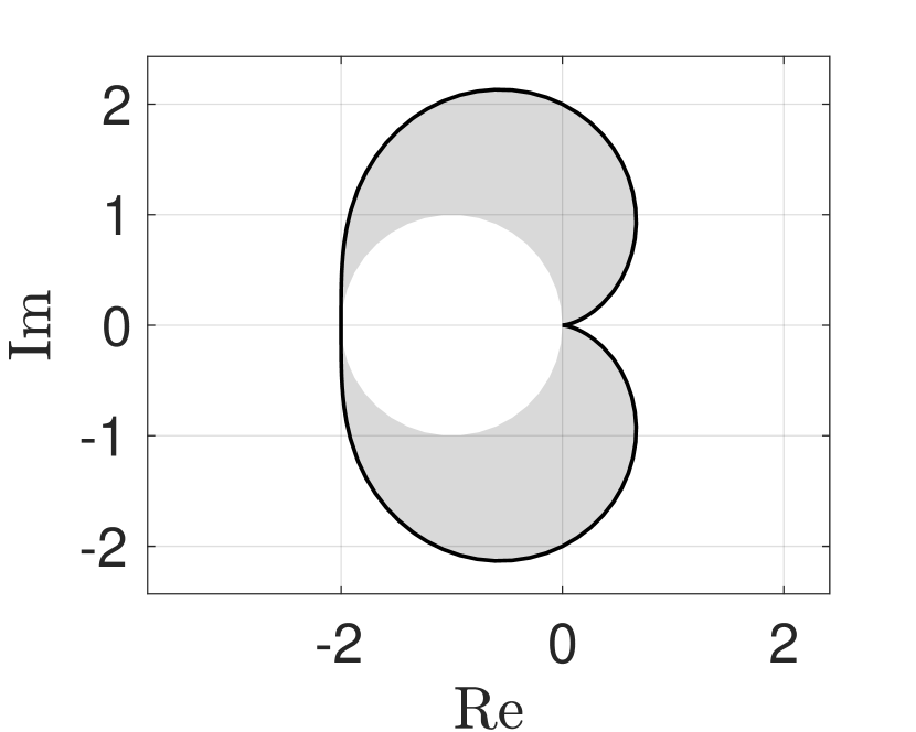
(a) $\operatorname{SRG}(L)$.

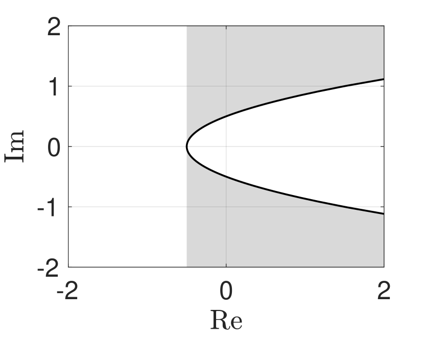
(b) $\operatorname{SRG}(L)^{-1}$.

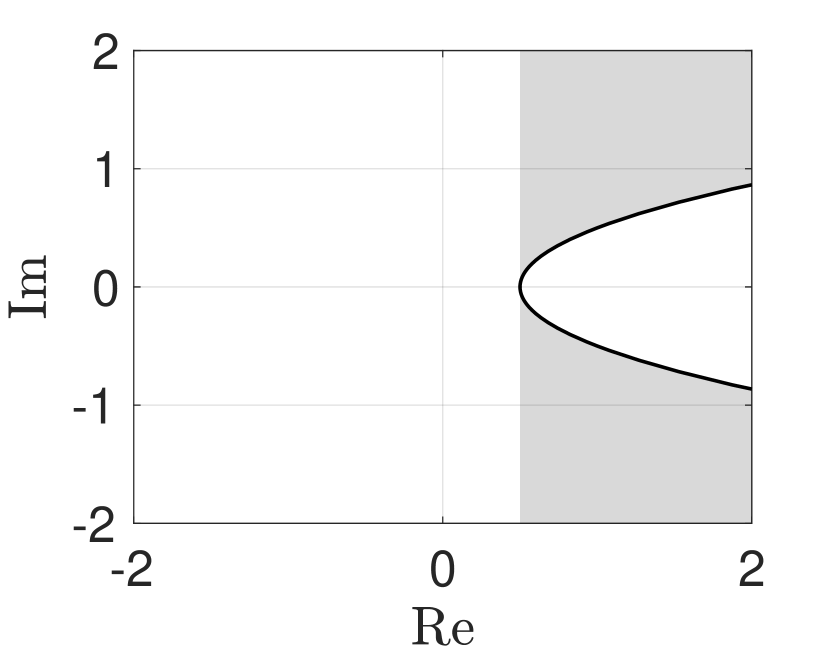
(c) $1+\operatorname{SRG}(L)^{-1}$.

(d) $\operatorname{SRG}(T)$.

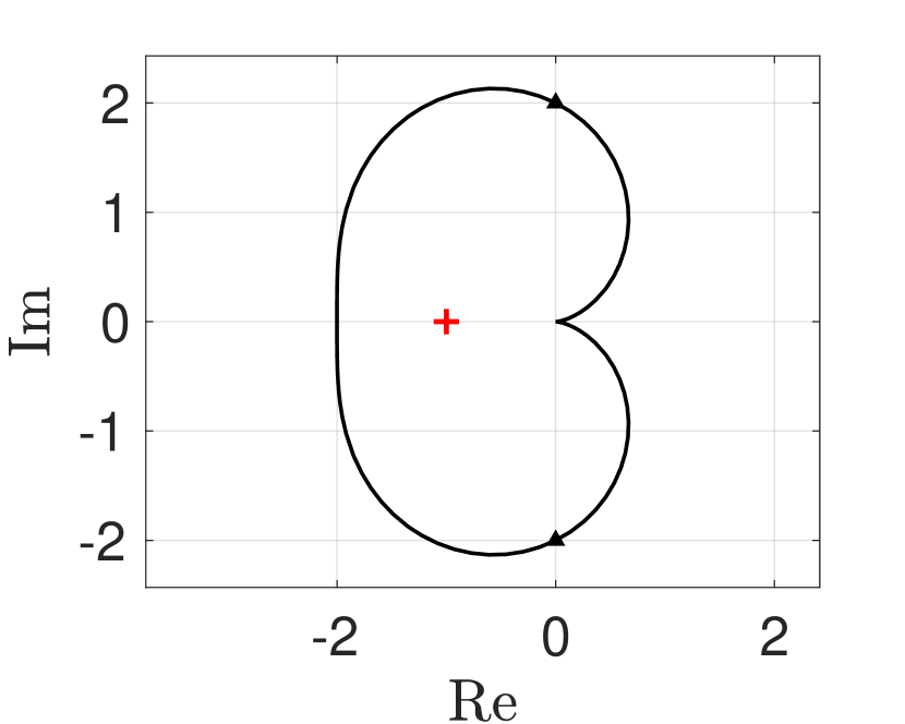
(e) $\operatorname{Nyquist}(L)$.

Figure 4: SRGs and Nyquist diagram corresponding to $L(s)=\frac{-2}{s^{2}+s+1}$. The shaded area is the SRG and the bold line is the Nyquist diagram.

However, when one uses the Nyquist stability criterion Theorem 1 to analyze stability, one concludes that $T(s)$ is unstable. This can be seen from the Nyquist diagram in Fig. 4(e), which encircles $-1$ one time in clockwise fashion, which results in $Z=1$ in Theorem 1, indicating that $T(s)$ has one unstable pole.

It appears that we have derived a contradiction. Nyquist theory correctly predicts instability, and we have applied the rules of SRG calculus in a correct manner, but still derived a wrong result.

This apparent dichotomy is reminiscent of the Nyquist diagram of an unstable plant. When an LTI plant is continuously transformed from a stable to an unstable plant, the Nyquist diagram only achieves infinite radius at the transition point between stable and unstable behavior. An example is $T_{a}(s)=1/(s+a)$, which is stable for $a>0$, unstable for $a<0$, and achieves infinite radius only at the transition point $a=0$.

For LTI systems, the fact that the radius only attains infinity at a transition point is not a problem, since we can use the Nyquist criterion to assess stability. For SRGs, however, we do not have access to this information.

Before we explain the solution, we elaborate a bit more on this pitfall, and the SRG of an unstable LTI operator.

IV-B Understanding the Pitfalls

With the current SRG formulas, the SRG radius blows up only at the transition point between stable and unstable. Therefore, direct application of SRG formulas, i.e. not using homotopy arguments that start from a stable system, can lead to “false positives” that incorrectly predict a stable system. This means that the bound for the incremental $L^{2}$-gain is only valid if we know a priori that the system is stable, or part of an internally stable feedback loop, analogous to the maximum gain that the Nyquist curve predicts.

When dealing with a Nyquist curve, however, one can count encirclements of $-1$ to check stability. This circle counting is not available for the h-convex hull of a Nyquist curve, since the frequency information is thrown away, and we only have a set of complex numbers.

Now it can be understood why Theorem 4 requires stability to begin with, and uses a homotopy argument. It is not only to guarantee well-posedness, but also to prevent “false positive” predictions.

IV-C The SRG of an Unstable LTI System

We know the exact SRG of a stable LTI operator via Theorem 3. One could argue that this theorem can be extended to marginally stable operators, i.e., those containing integrators, using a limiting argument where poles are represented as $\lim_{a\downarrow 0}1/(s+a)$. However, it is unclear how to compute the SRG of an unstable LTI operator.

For an unstable LTI plant, the Nyquist diagram, or the Bode diagram for that matter, can only be interpreted as gain and phase per frequency information if the unstable plant as part of an internally stable feedback system. That is, the plant only receives signals that stabilize the plant. Denote $\mathcal{U}\subset L^{2}_{e}$ the set of signals that stabilize the unstable LTI plant $L$. Then it is clear that $\operatorname{SRG}_{\mathcal{U}}(L)$ is the h-convex hull of $\operatorname{Nyquist}(L)$. This is precisely what is obtained in Fig. 4(d), which is $\operatorname{SRG}_{\mathcal{U}}(T)$, where $\mathcal{U}$ is the set of signals that stabilize $T$. This case is an example of where the SRG constrained to some input space is used. Here, it misleads us since we had that impression that we studied the stability on $L^{2}_{e}$, whereas we actually only considered $\mathcal{U}$.

V Resolution of Pitfalls

The fundamental reason of the pitfalls reported is that the SRG disregards the information provided by the Nyquist criterion. As a resolution of these pitfalls, we prove that the Nyquist criterion can be combined with the SRG, such that direct application of SRG calculus leads to consistent results.

V-A Main result

Before stating our main result, we need the following definition.

Definition 1.

Let $R$ be an LTI operator with $P$ poles with $\real(p)>0$. Denote $\mathcal{G}_{R}$ as the h-convex hull of $\operatorname{Nyquist}(R)$ and denote

$$\mathcal{N}_{R}^{+}=\{z\in\mathbb{C}\mid N_{R}(z)+P>0\},$$ (6)

where $N_{R}(z)$ denotes the amount of encirclements of $z$ by $\operatorname{Nyquist}(R)$ and let

$$\mathcal{N}_{R}=\{z\in\mathcal{N}_{R}^{+}\mid z\text{ is path connected to }\mathbb{R}\text{ in }\mathcal{N}_{R}^{+}\}.$$ (7)

Define the extended SRG of an LTI operator as

$$\operatorname{SRG}^{\prime}(R):=\mathcal{G}_{R}\cup\mathcal{N}_{R}.$$ (8)

Theorem 5.

Under the condition that $\operatorname{SRG}(\phi)$ obeys the chord property and there exists some $\kappa\in\mathbb{R}$ such that $\kappa\in\operatorname{SRG}(\phi)$ and for all $0\leq\tau_{1}\leq\tau_{2}\leq 1$, it holds that

$$\tau_{1}\left(\operatorname{SRG}(\phi)-\kappa\right)\subseteq\tau_{2}\left(\operatorname{SRG}(\phi)-\kappa\right).$$ (9)

Then, the system is a well-posed operator $T:L^{2}_{e}\to L^{2}_{e}$ in the sense of existence, uniqueness, continuity, causality, and boundedness, and it is stable if

$$0\notin\operatorname{SRG}^{\prime}(G)^{-1}+\operatorname{SRG}(\phi).$$

Proof.

Consider the system in Fig. 2, for which the complementary sensitivity operator reads $T=(G^{-1}+\phi)^{-1}$. By assumption, we can pick some real $\kappa\in\operatorname{SRG}(\phi)$. Upon replacing $\phi$ with $\kappa$, we obtain the LTI complementary sensitivity transfer function $T(s)=(1+\kappa G(s))^{-1}G(s)$. For $\tau\in[0,1]$, define $T_{\tau}=(G^{-1}+\kappa+\tau(\phi-\kappa))^{-1}$. Stability of $T_{0}=T(s)$ is assessed using the Nyquist stability criterion by counting the encirclements of $-1/\kappa$ by $G(j\omega)$. Note that $\mathbb{R}\cap\operatorname{SRG}^{\prime}(G)=\mathbb{R}\cap(\mathcal{N}_{G}\cup\operatorname{Nyquist}(G))$, hence if $-1/\kappa\in\operatorname{SRG}^{\prime}(G)$ holds, stability is solely determined by the Nyquist criterion.

Suppose $-1/\kappa\in\operatorname{SRG}^{\prime}(G)$, then we are in one of two situations.

• $-1/\kappa\in\operatorname{Nyquist}(G)$, in which case $T(s)$ is marginally stable since it has an integrator. We classify this situation as unstable, as the system is not BIBO stable

• $-1/\kappa\in\mathcal{N}_{G}$, in which case we know from Theorem 1 that $T(s)$ has at least one unstable pole.

In both cases, we end up with $0\in\operatorname{SRG}^{\prime}(G)^{-1}+\operatorname{SRG}(\phi)\supset\operatorname{SRG}(G^{-1}+\phi)$, i.e., we cannot prove that $T$ is stable using SRG calculus.

Now suppose $-1/\kappa\notin\operatorname{SRG}^{\prime}(G)$. In this case, we know from Theorem 1 that $T(s)$ is stable. We now continuously transform $\kappa$ to $\phi$, by letting $\tau$ run from $0$ to $1$ in $\kappa+\tau(\phi-\kappa)$. By assumption Eq. (9), $-\operatorname{SRG}^{\prime}(G)^{-1}\cap\operatorname{SRG}(\phi)=\emptyset$ guarantees $-\operatorname{SRG}^{\prime}(G)^{-1}\cap\operatorname{SRG}(\kappa+\tau(\phi-\kappa))=\emptyset$ for all $\tau\in[0,1]$, such that stability and well-posedness is maintained for all $\tau\in[0,1]$ [8]. Therefore, if $-\operatorname{SRG}^{\prime}(G)^{-1}\cap\operatorname{SRG}(\phi)=\emptyset$, then we know $T$ has finite incremental $L^{2}$-gain, upper bounded by the radius of $(\operatorname{SRG}^{\prime}(G)^{-1}+\operatorname{SRG}(\phi))^{-1}$, which is the over-approximation of $\operatorname{SRG}(T)$ as obtained via the rules of SRG calculus. This completes the proof. ∎

V-B The Generalized Circle Criterion

Theorem 4 can only reproduce the circle criterion in the case that $G$ in Fig. 2 is stable. We will now show that using our result, Theorem 5, one can prove a result that is more general than the celebrated circle criterion by Theorem 2. We emphasize that this is possible since we combined the information of the Nyquist criterion into the SRG.

Theorem 6.

Let $G(s)$ be an LTI operator and $\phi$ a nonlinear operator. The Lur’e system $T=(G^{-1}+\phi)^{-1}$ in Fig. 2 has finite $L^{2}$-gain and satisfies $r\in L^{2}_{e}\implies y\in L^{2}_{e}$ if

$$-\operatorname{SG}_{0}(\phi)^{-1}\cap\operatorname{SRG}^{\prime}(G)=\emptyset.$$ (10)

Furthermore, we have the bound $\norm{T}_{L^{2}_{e}}\leq 1/r_{m}$, where $r_{m}$ is the minimal distance between $-\operatorname{SG}_{0}(\phi)$ and $\operatorname{SRG}^{\prime}(G^{-1})$.

One can replace $L^{2}$-gain with incremental $L^{2}$-gain by taking $\operatorname{SRG}(\phi)$ instead of $\operatorname{SG}_{0}(\phi)$ in (10).

Proof.

The theorem is a direct result of Theorem 5 upon realizing that $-\operatorname{SG}_{0}(\phi)\cap\operatorname{SRG}^{\prime}(G)^{-1}=\emptyset$ is equivalent to (10). ∎

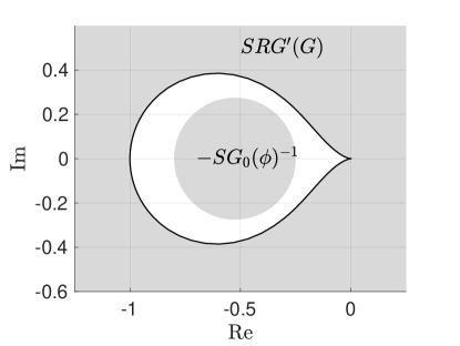
Figure 5: Generalization of the circle criterion using SRGs. The black curve is $\operatorname{Nyquist}(G)$ and the grey regions display sets in Eq. (10).

Note that Theorem 6 is equivalent to the circle criterion in Theorem 2 when $\phi\in[k_{1},k_{2}]$. However, it is more general than the circle criterion since $\phi$ can be any operator, not necessarily sector bounded. Additionally, SRG analysis provides a bound on the (incremental) $L^{2}$-gain of the system, whereas the classical circle criterion only guarantees boundedness and stability.

Remark 1.

One might worry that the h-convex hull of the Nyquist diagram will make the SRG analysis more conservative than the circle criterion. We will argue here that this is not the case. Recall that $D_{[k_{1},k_{2}]}$ is a disk centered on the real line, hence so is $D_{[-1/k_{1},,-1/k_{2}]}=:D_{\phi}$. Suppose that the h-convex hull does make the SRG analysis more conservative, i.e.

$$D_{\phi}\cap\operatorname{Nyquist}(G)=\emptyset,$$ (11)

$$D_{\phi}\cap\operatorname{SRG}(G)\neq\emptyset,$$

are both true. Note that we use the SRG for $G$ as defined in Theorem 3, so we only consider the h-convex hull part. If (11) would be true, then there exist $z_{1},z_{2}\in\operatorname{Nyquist}(G)\cap\mathbb{C}_{\imaginary>0}$ such that $z_{1},z_{2}\notin D_{\phi}$, but $\operatorname{Arc}_{\text{min}}(z_{1},z_{2})\cap D_{\phi}\neq\emptyset$. This is only possible if either $z_{1}$ or $z_{2}$ lies in $D_{\phi}$, since $D_{\phi}$ is already h-convex. This contradicts (11), and therefore the statement is false and we can conclude that the h-convex hull does not make the SRG analysis of the Lur’e system more conservative than the circle criterion.

VI Example: Duffing Oscillator

Our example, the Duffing oscillator, showcases the application of Theorem 5 to a Lur’e system as shown in Fig. 2. It also shows how the SRG analysis is applied to restricted input spaces.

VI-A Duffing Oscillator

The Duffing oscillator is defined by the ODE

$$\ddot{y}+\delta\dot{y}+\alpha y+\beta y^{3}=u(t),$$ (12)

where $\alpha,\beta,\delta\in\mathbb{R}$ are parameters and $u(t)\in L^{2}_{e}$ is some input signal. It can be viewed as a mass-spring-damper system with nonlinear spring. The particular choice of parameters in this work is $\alpha=-1,\,\beta=1$, and $\delta=0.3$. The control objective we consider is to stabilize the origin w.r.t. the input $r=0$ and process noise $d$, see Fig. 6. We assume that the disturbance obeys $\norm{d}_{\infty}\leq 1$. The chosen controller is a PD controller.

Figure 6: Block diagram of process disturbance for controlled Lur’e systems.

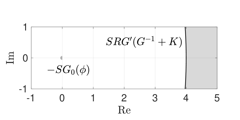
(a) SRG analysis with $\norm{y}_{\infty}=0.25$.

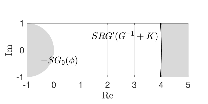
(b) SRG analysis with $\norm{y}_{\infty}=\sqrt{2}$.

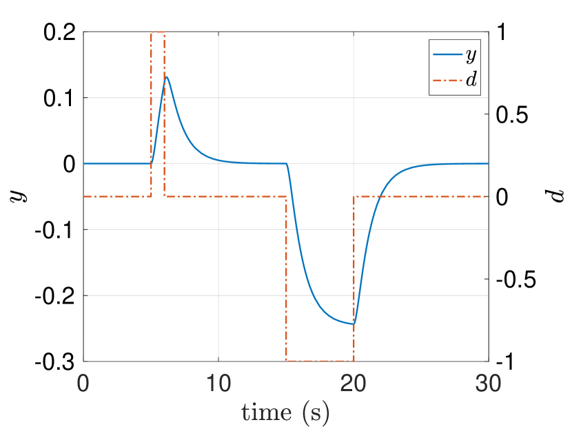
(c) Simulation response with disturbance.

Figure 7: Analysis of the Duffing oscillator with process disturbance.

VI-B SRG Analysis

In order to write the Duffing system in the form of Fig. 6, we rewrite Eq. (12) as as a Lur’e system with $G(s)=1/(s^{2}+\delta s+\alpha)$ and $\phi(y)=\beta y^{3}$. The controller $K(s)=k_{p}+k_{d}s/(s/N+1)$ is the PD controller. It turns out that Fig. 6 can be written in the Lur’e form in Fig. 2 by setting $r=d$ and replacing $G$ with $G/(1+GK)$. This can be seen from the relation $y=(G^{-1}+K+\phi)^{-1}d$ and comparing with Eq. (4).

Note that $\operatorname{SRG}(\phi)$ is problematic, since $\operatorname{SRG}(\phi)=\mathbb{C}_{\real>0}$. Now, consider an upper bound $\norm{y}_{\infty}\leq M$, which can be obtained for the Duffing oscillator based on the approach detailed in Appendix A. For values $k_{p}=k_{d}=5$ and $N\to\infty$, the bound reads $\norm{y}_{\infty}\leq 0.25$. Since we study the behavior w.r.t the zero solution $r=d=0$, we can use the scaled graph around zero. This gives us $\operatorname{SG}_{0}(\phi)\subset\{z\in\mathbb{C}_{\real>0}\mid|z|\leq\norm{y}_{\infty}^{2}\}$.

The $L^{2}$-gain of the process sensitivity $PS:d\mapsto y$ is given by $1/r_{PS}$, where $r_{PS}$ is the smallest distance between $-\operatorname{SG}_{0}(\phi)$ and $\operatorname{SRG}^{\prime}(G^{-1}+K)$. See Fig. 7(a) for the SRG analysis, where $N=100$ is used for the PD controller. We can read off $\norm{PS}_{L^{2}_{e}}\approx 1/4$.

Instead of estimating an upper bound for $\norm{y}_{\infty}$, one can design the controller for the operating range $y\in[-\sqrt{2},\sqrt{2}]$, as done in [10]. This allows one to use $\operatorname{SRG}(\phi)=D_{[0,6\beta]}$ and $\operatorname{SG}_{0}(\phi)=D_{[0,2\beta]}$ directly in SRG calculations. This bound is used in Fig. 7(b), where a bound $\norm{PS}_{L^{2}_{e}}\approx 1/4$ is obtained, analogous to the result from Fig. 7(a).

VI-C Simulation Results

The disturbed Duffing oscillator is simulated on the time interval $t\in[0,30]$ for the parameters $\alpha=-1,\,\beta=1,\,\delta=0.3$ and controller parameters $k_{p}=k_{d}=5,\,N=100$. At $t=5$ we apply $d=1$ for one second and at $t=15$ we apply $d=-1$ for five seconds. The results are plotted in Fig. 7(c). We see that indeed the response of the system is at most $1/4$ the size of the disturbance (see $t=20$), which corresponds to $\norm{PS}_{L^{2}_{e}}\approx 1/4$.

VII Conclusion and Outlook

We have shown how to combine the Nyquist criterion with the SRG in order to use SRG analysis with unstable LTI plants. One immediate result is the generalized circle criterion, and we have shown its application to disturbance rejection analysis for the Duffing oscillator.

We focused on the Lur’e setup beyond sector bounded nonlinearities, for which we also guarantee well-posedness in the sense of [8]. Topic of further research is to generalize Theorem 5 to more general feedback interconnections, preferably while preserving well-posedness, to fully remove the limitation of current SRG methods.

Appendix A Bound for the Duffing Oscillator

In this appendix, we show how obtains a bound $\norm{y}_{\infty}$ for the system in Fig. 6. The system with a pure PD controller $K=k_{p}+k_{d}s$ can be written as $\ddot{y}=-\tilde{\alpha}y-\beta y^{3}-\tilde{\delta}\dot{y}+d$, where $\tilde{\alpha}=\alpha+k_{p}>0$ and $\tilde{\delta}=\delta+k_{d}>0$. Using $\tilde{\delta}=0$ and $d=0$, we can define the Hamiltonian $H(y,\dot{y}):=\frac{1}{2}(\dot{y})^{2}+\frac{1}{2}\tilde{\alpha}y^{2}+\frac{1}{4}\beta y^{4}$, which reproduces the Duffing equation upon the substitution $x=\dot{y}$ with $\dot{y}=\partial H/\partial x,\ddot{y}=\dot{x}=-\partial H/\partial y$. This Hamiltonian is a convex potential, consisting of a linear and cubic spring, both with positive spring constant. Therefore, the maximum amplitude $\norm{y}_{\infty}$ of the system is monotone increasing with the energy $H$, which in turn means that disturbance $d$ that maximizes $H$ will result in the upper bound for $\norm{y}_{\infty}$.

Multiplying the Duffing equation by $\dot{y}$ result in the equality $\dot{y}(\ddot{y}+\tilde{\alpha}y+\beta y^{3}+\tilde{\delta}\dot{x}-d(t))=0$, which can be rewritten as $\frac{\differential}{\differential t}H(y,\dot{y})=-\tilde{\delta}(\dot{y})^{2}+\dot{y}d(t)$. This means that $d(t)$ should always have the same sign as $\dot{y}$ in order to add as much energy to the system as possible.

If the system at $t=0$ starts at $(y,\dot{y})=(\norm{y}_{\infty},0)$ with $d=\norm{d}_{\infty}$ throughout, then the turning point should obey $(y,\dot{y})=(\norm{y}_{\infty},0)$. Solving this problem numerically for the values $\alpha=-1,\,\beta=1,\delta=0.3$, $k_{p}=k_{d}=5$, and $\norm{d}_{\infty}=1$, the resulting bound is $\norm{y}_{\infty}=0.25$.

References

- [1] H. Nyquist, “Regeneration Theory,” Bell System Technical Journal, vol. 11, no. 1, pp. 126–147, 1932.
- [2] I. W. Sandberg, “A Frequency-Domain Condition for the Stability of Feedback Systems Containing a Single Time-Varying Nonlinear Element,” Bell System Technical Journal, vol. 43, no. 4, pp. 1601–1608, 1964.
- [3] N. M. Krylov, N. N. Bogoliubov, and S. Lefschetz, Introduction to Non-Linear Mechanics, ser. Annals of Mathematics Studies; No. 11. Princeton University Press, 1947.
- [4] A. Pavlov, N. Van De Wouw, A. Pogromsky, M. Heertjes, and H. Nijmeijer, “Frequency domain performance analysis of nonlinearly controlled motion systems,” in Proc. of the 2007 46th IEEE Conference on Decision and Control. IEEE, 2007, pp. 1621–1627.
- [5] E. K. Ryu, R. Hannah, and W. Yin, “Scaled relative graphs: Nonexpansive operators via 2d Euclidean geometry,” Mathematical Programming, vol. 194, no. 1, pp. 569–619, 2022.
- [6] T. Chaffey, F. Forni, and R. Sepulchre, “Graphical Nonlinear System Analysis,” IEEE Transactions on Automatic Control, vol. 68, no. 10, pp. 6067–6081, 2023.
- [7] S. Van Den Eijnden, T. Chaffey, T. Oomen, and W. (Maurice) Heemels, “Scaled graphs for reset control system analysis,” European Journal of Control, p. 101050, 2024.
- [8] A. Megretski and A. Rantzer, “System analysis via integral quadratic constraints,” IEEE Transactions on Automatic Control, vol. 42, no. 6, pp. 819–830, 1997.
- [9] C. A. Desoer and M. Vidyasagar, Feedback Systems: Input-Output Properties, ser. Electrical Science Series. New York: Acad. Press, 1975.
- [10] P. J. Koelewijn, S. Weiland, and R. Tóth, “Equilibrium-independent control of continuous-time nonlinear systems via the lpv framework–extended version,” arXiv preprint arXiv:2308.08335, 2023.