[a,b]Stephan Dürr
Taste-splittings of staggered, Karsten-Wilczek and Borici-Creutz fermions under gradient flow in 2D
Abstract
Karsten-Wilczek and Borici-Creutz fermions show a near-degeneracy of the species involved, similar to the species of staggered fermions. Hence in dimensions all three formulations happen to be minimally doubled (two species). This near-degeneracy shows up both in the eigenvalue spectrum of the respective Dirac operator and in spectroscopic quantities (e.g. the pion mass), but in the former case it is easier to quantify. We use the quenched Schwinger model to determine the low-lying eigenvalues of these fermion operators at a fixed gradient flow time (either in lattice units or in physical units, hence keeping either or fixed at all ).
1 Introduction
Taste splittings are an unwanted effect – a lattice artefact or “cut-off effect”. They are genuine to any lattice fermion action involving more than one species (a.k.a. “doubled action”).

For instance staggered fermions involve species in space-time dimensions (i.e. 2 species or “tastes” in 2D, and 4 in 4D). This is visible in the eigenvalue spectrum of ; instead of one continuum eigenvalue one finds a pair (in 2D) or a quartet (in 4D) of near-degenerate eigenvalues on a representative gauge background [3, 4]. Accordingly, in a dynamical simulation with one field of the well-known rooting procedure effectively replaces each pair (quartet) by the geometric mean of the two (four) multiplet eigenvalues in 2D (4D).
More recently, Karsten-Wilczek (KW) [5, 6] and Borici-Creutz (BC) [7, 8] fermions were proposed, since they entail only two species. This is just the minimum number required by the Nielsen-Ninomyia theorem (and hence the same number in 2D and 4D). As a result, in 4D one can simulate QCD with KW or BC fermions without using the rooting trick.
Specifically in 2D, not just KW and BC fermions, but also staggered fermions happen to be “minimally doubled”. Accordingly, the Schwinger model (QED in 2D) is well suited to compare the taste-breaking effects of these three fermion formulations to each other. There are two options for addressing the taste breaking effects. One may determine spectrosopic quantities like , where the second subscript indicates the taste structure of the pion. Or one may measure the above mentioned eigenspectra and determine the splitting within each pair.
Today it is common practice to evaluate the Dirac operator on a gauge background which is derived from the actual configuration via a few steps of stout smearing [9] or some gradient flow evolution [10, 11]. At first sight the difference between these smoothings procedures is small, since the correspondence (see e.g. [12] and references therein) says that the flow time in lattice units (r.h.s.) equals the cumulative sum of the stout parameters used (l.h.s.).
The effect of 1 or 3 stout steps on the eigenvalues of , and has been investigated in Ref. [13]. Here we take first steps towards exploring the effect of the gradient flow.
2 Effect of the gradient flow on gluonic quantities
In the two-dimensional theory one defines where is the lattice site and the complex conjugate of . Using the parametrization one may write with the plaquette angle, mapped to the interval , given by .
The Wilson action is and another option is . Two definitions of the topological charge are in common use, the geometric charge and optionally .
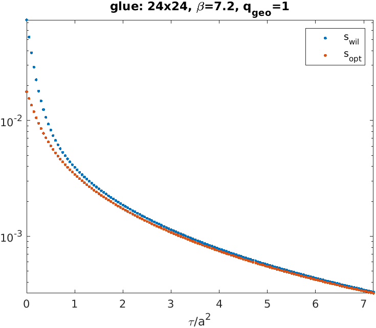
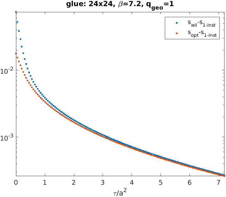
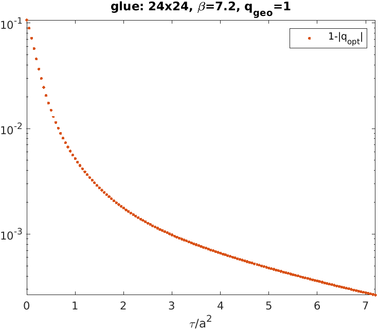
We choose a thermalized gauge configuration at , and plot and versus the flow time in the interval in Fig. 1. It seems that and for large , as expected. Fortunately, the -instanton configuration in the Schwinger model is known analytically [14]; its action is . Hence, by subtracting from either observable its value, we can study the asymptotic ascent. Fig. 2 suggests that for and the asymptotic value is assumed exponentially in the flow time .
| 3.2 | 5.0 | 7.2 | 12.8 | 20.0 | 28.8 | 51.2 | |
| 16 | 20 | 24 | 32 | 40 | 48 | 64 | |
| 3.2 | 5.0 | 7.2 | 12.8 | 20.0 | 28.8 | 51.2 |
We checked the effect that larger/smaller boxes at the same coupling have; we found no significant change. In the Schwinger model varying the lattice spacing at fixed physical box size is simple, if is set through the dimensionful coupling , since . This allows us to compile a list of matched lattices/flow-times before running any simulation, see Tab. 1.
| 3.2 | 5.0 | 7.2 | 12.8 | 20.0 | 28.8 | 51.2 | |
|---|---|---|---|---|---|---|---|
| at | 3e-3 | 1e-3 | 1e-3 | 3e-4 | 3e-4 | 1e-4 | 1e-4 |
| at | 1e-5 | 1e-8 | 1e-10 | 1e-12 |
3 Effect of the gradient flow on Dirac operator eigenvalues
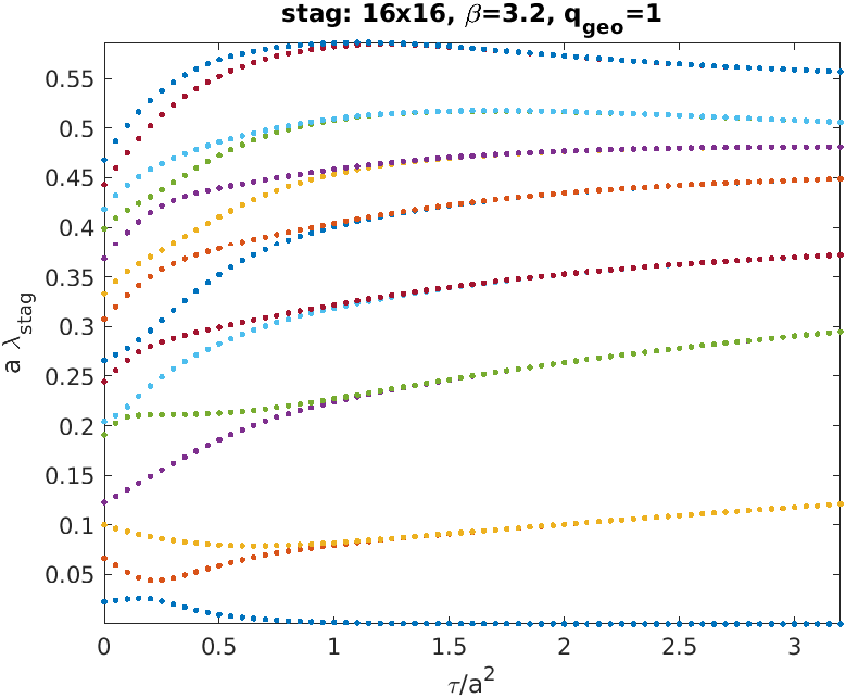
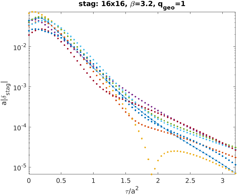
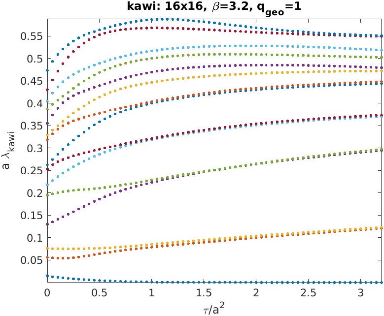
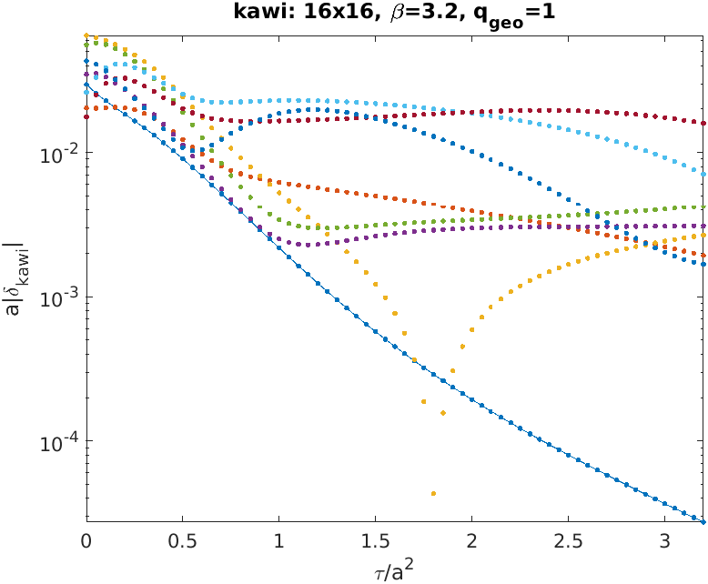
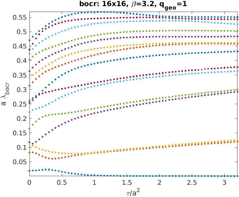
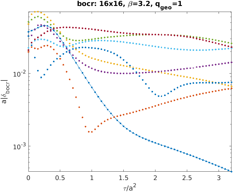
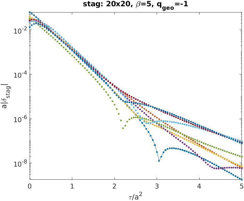
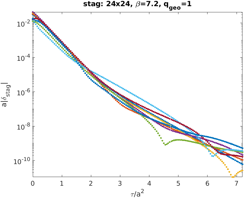
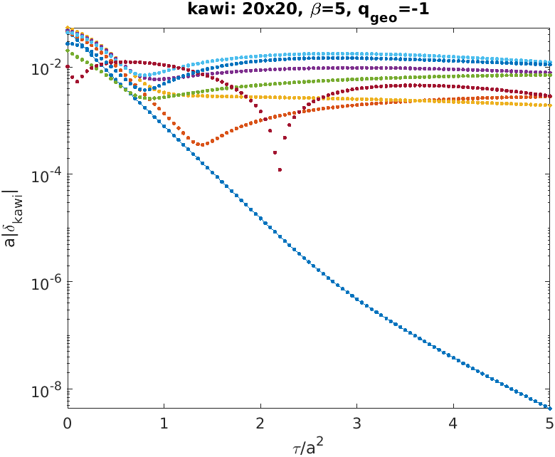
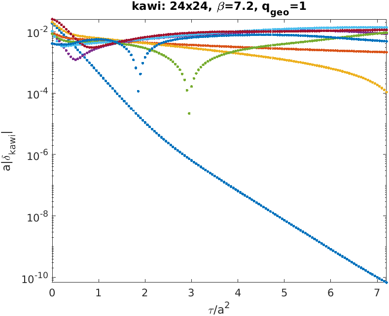
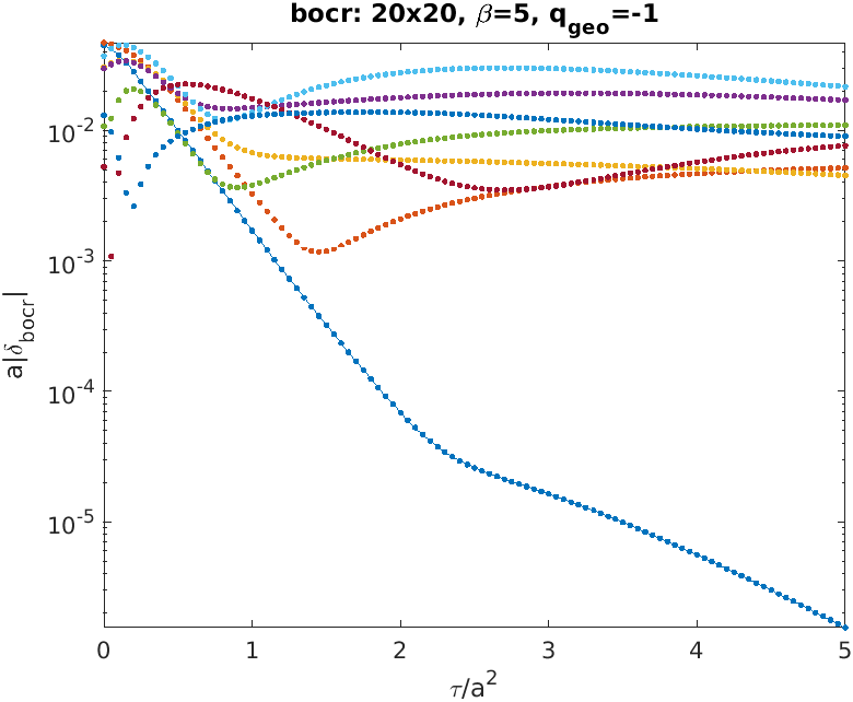
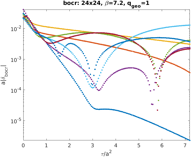
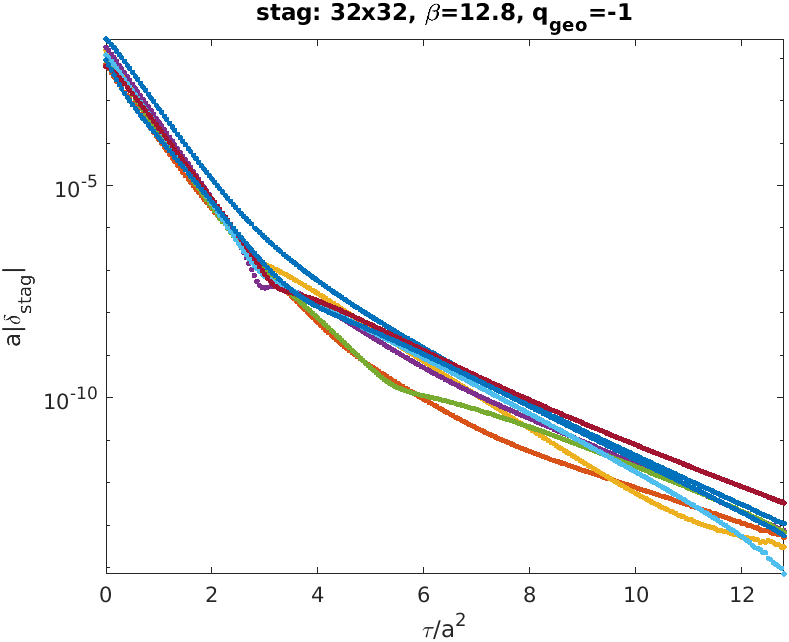
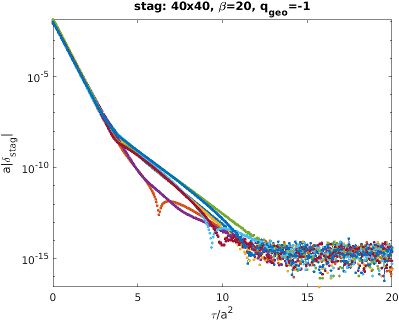
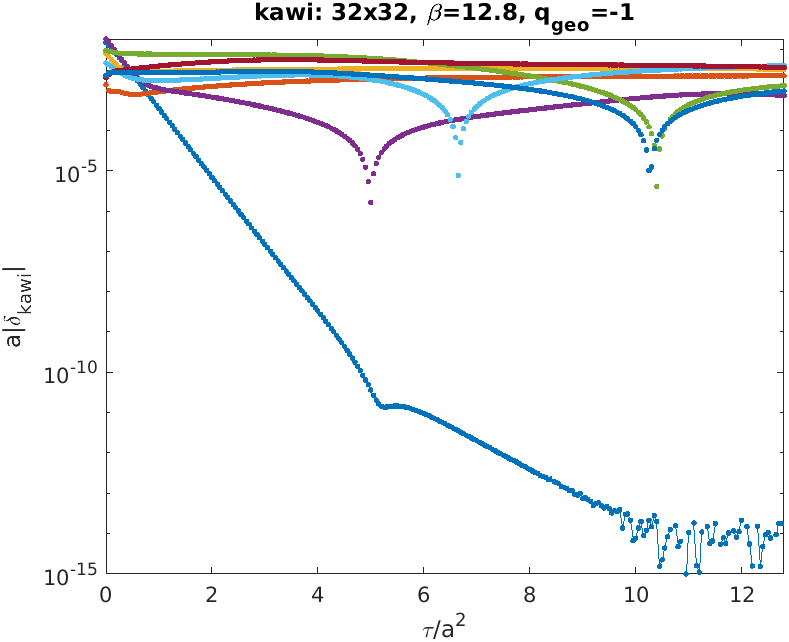
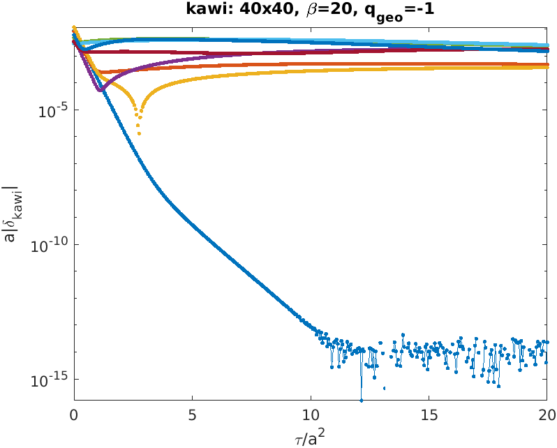
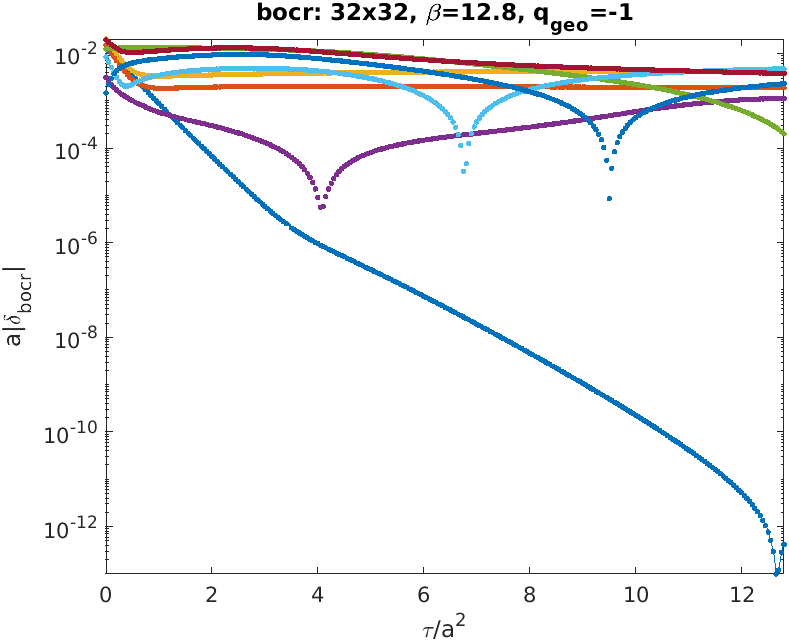
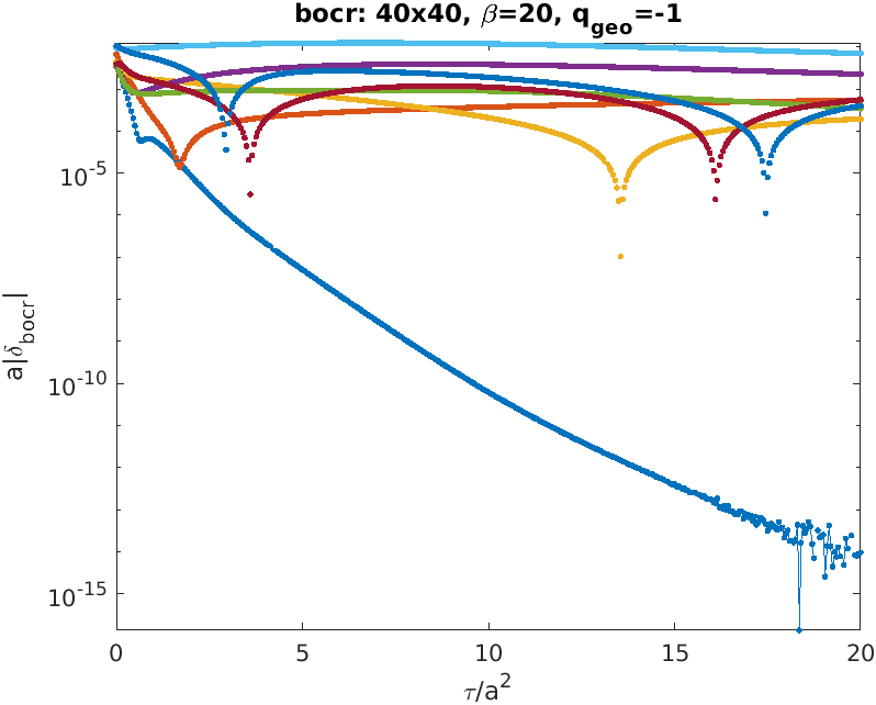
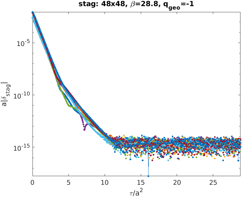
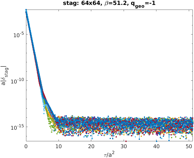
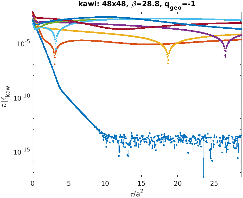
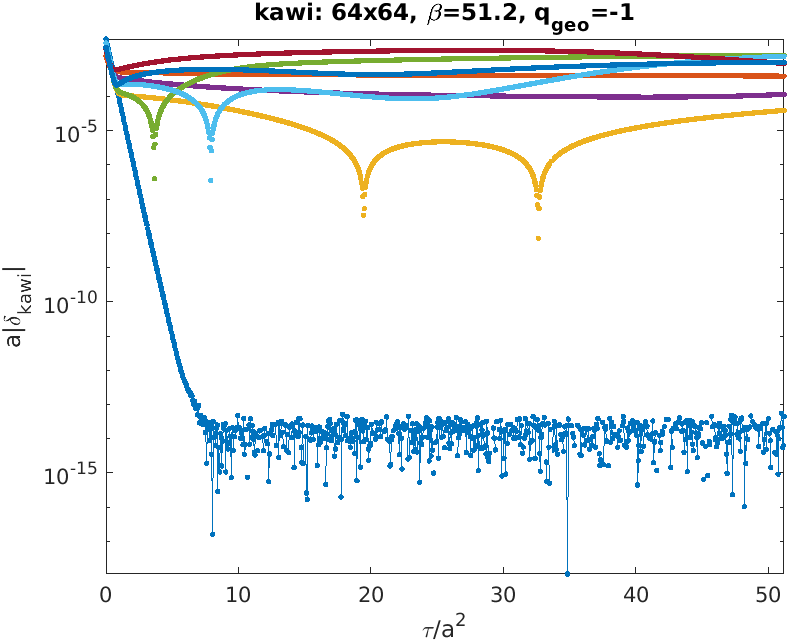
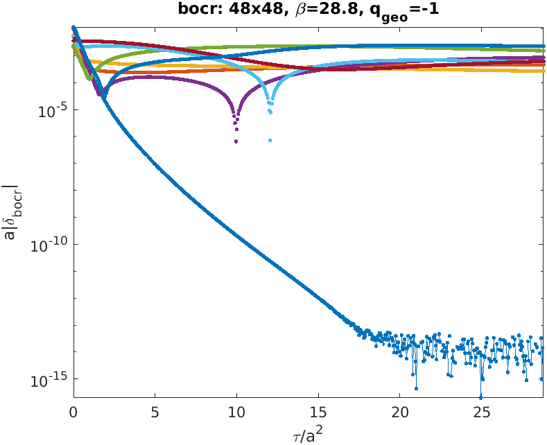
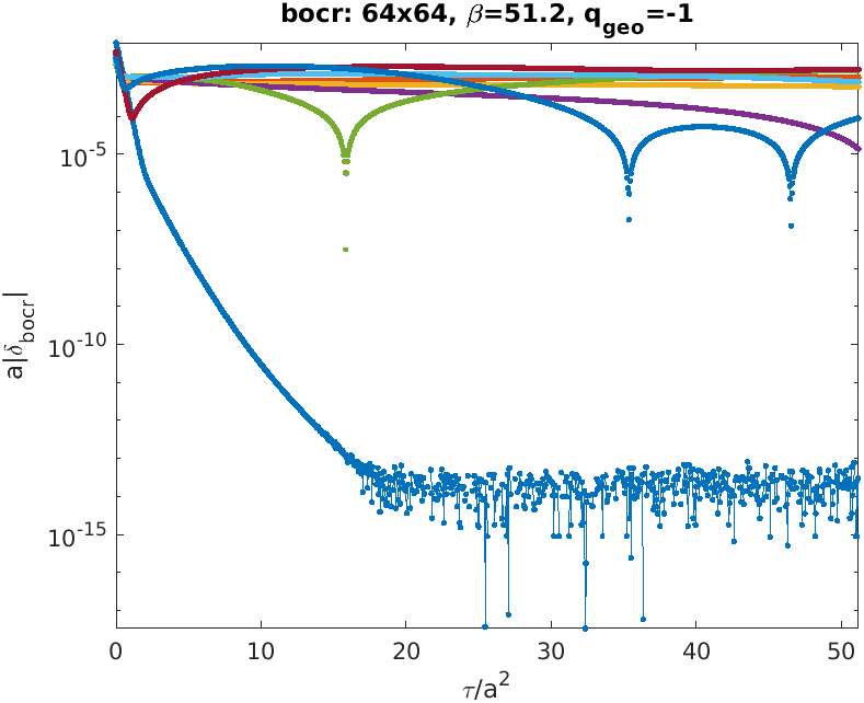
The massless staggered Dirac operator has purely imaginary eigenvalues which come in pairs , due to -hermiticity. In Fig. 3 we plot the 15 smallest imaginary parts on the original background at . At this stage, no pairing is visible. Only as we repeat this for smoothed backgrounds , the pairing becomes visible at . The staggered taste splittings (e.g. , for , see Ref. [13]) all seem to decline exponentially in . For KW and BC fermions, the situation is similar for the pair (which is the would-be zero-mode pair for ), while all non-topological mode splittings diminish only reluctantly.
In Fig. 4 we repeat this for , in Fig. 5 for , and in Fig. 6 for . Throughout, we select a single representative configuration with topological charge . What changes is the maximum flow-time in lattice units, in line with Tab. 1. Beginning at double precision may be insufficient to resolve the smallest taste splitting.
To summarize one may say that increasing in a fixed physical volume did not bring any significant change. The would-be zero-mode splitting decreases roughly exponentially for each formulation. But the non-topological zero-mode splittings diminish in this way only in the staggered case, while they reach values in the KW/BC cases. For staggered fermions it is interesting to compare at fixed flow-time in lattice/physical units across , see Tab. 2.
4 Conclusions
KW and BC fermions distinguish between would-be zero-mode splittings (which decrease exponentially in the gradient flow time) and non-topological mode splittings (which do not). By contrast, staggered fermions reduce their taste breakings exponentially with the flow time, regardless of the nature of the underlying continuum mode. The good news for staggered practitioners is that all taste splittings disappear when at least one of the limits is taken.
It will be interesting to extend this investigation to ensembles at various combinations, keping the physical box size fixed as in Ref. [13]. The gradient flow allows for two smoothing strategies: the flow time may be kept fixed in lattice units () or in physical units ( in 2D), see Tabs. 1 and 2. In the first case, locality of the fermion formulation in the continuum limit is guaranteed by construction (as is true with any fixed number of stout steps). In the second case, locality is an issue but the lattice regulator gets replaced by a diffusive regulator with universal properties [10, 11] (see also the discussion in Ref. [12]).
An issue not addressed so far is the admixture of lower-dimensional operators to and [15, 16, 17], as the respective coefficients are not known in 2D. We plan to embark on such a calculation; with such numbers in hand one can try to compensate these mixing effects. Perhaps, with correct unmixing, a future version of our KW/BC taste splitting plots might look different ?
References
- [1]
- [2]
- [3] E. Follana, A. Hart and C. T. H. Davies, Phys. Rev. Lett. 93, 241601 (2004) [hep-lat/0406010].
- [4] S. Dürr, C. Hoelbling and U. Wenger, Phys. Rev. D 70, 094502 (2004) [arXiv:hep-lat/0406027].
- [5] L. H. Karsten, Phys. Lett. 104B, 315 (1981).
- [6] F. Wilczek, Phys. Rev. Lett. 59, 2397 (1987).
- [7] M. Creutz, JHEP 0804, 017 (2008) [arXiv:0712.1201 [hep-lat]].
- [8] A. Borici, Phys. Rev. D 78, 074504 (2008) [arXiv:0712.4401 [hep-lat]].
- [9] C. Morningstar and M.J. Peardon, Phys. Rev. D 69, 054501 (2004) [arXiv:hep-lat/0311018].
- [10] M. Lüscher, JHEP 08, 071 (2010) [erratum: ibid 03, 092 (2014)] [arXiv:1006.4518 [hep-lat]].
- [11] M. Lüscher and P. Weisz, JHEP 02, 051 (2011) [arXiv:1101.0963 [hep-th]].
- [12] M. Ammer and S. Dürr, Phys. Rev. D 110, 054504 (2024) [arXiv:2406.03493 [hep-lat]].
- [13] M. Ammer and S. Dürr, submitted to Phys. Rev. D [arXiv:2409.15024 [hep-lat]].
- [14] J. Smit and J. C. Vink, Nucl. Phys. B 303, 36-56 (1988).
- [15] S. Capitani, M. Creutz, J. Weber, H. Wittig, JHEP 09, 027 (2010) [arXiv:1006.2009 [hep-lat]].
- [16] J. H. Weber, PoS LATTICE2023, 353 (2024) [arXiv:2312.08526 [hep-lat]].
- [17] D. A. Godzieba et al, PoS LATTICE2023, 283 (2024) [arXiv:2401.07799 [hep-lat]].