A RATIONAL KRYLOV METHODS FOR LARGE-SCALE LINEAR MULTIDIMENSIONAL DYNAMICAL SYSTEMS

H. Barkouki Ecole Nationale Supérieure d’Arts et Métiers, Meknès, Morocco. Email: h.barkouki@umi.ac.ma    K. Jbilou Université du Littoral, Côte d’Opale, batiment H. Poincarré, 50 rue F. Buisson, F-62280 Calais Cedex, France. University UM6P, Benguerir Morocco. Email: Khalide.Jbilou@univ-littoral.fr
Abstract

In this paper, we investigate the use of multilinear algebra for reducing the order of multidimensional linear time-invariant (MLTI) systems. Our main tools are tensor rational Krylov subspace methods, which enable us to approximate the system’s solution within a low-dimensional subspace. We introduce the tensor rational block Arnoldi and tensor rational block Lanczos algorithms. By utilizing these methods, we develop a model reduction approach based on projection techniques. Additionally, we demonstrate how these approaches can be applied to large-scale Lyapunov tensor equations, which are critical for the balanced truncation method, a well-known technique for order reduction. An adaptive method for choosing the interpolation points is also introduced. Finally, some numerical experiments are reported to show the effectiveness of the proposed adaptive approaches.

keywords:
Einstein product, Model recuction, Multi-linear dynamical systems, Tensor Rational Krylov subspaces, Lyapunov tensor equations.

1 Introduction

In this work, we develop methods based on projection onto block rational Krylov subspaces, for reducing the order of multidimensional linear time invariant (MLTI) systems.

Consider the following continuous time MLTI system

$$\left\{\begin{array}[]{c c c}\dot{\mathcal{X}}(t)&=&\mathcal{A}*\mathcal{X}(t)+\mathcal{B}*\mathcal{U}(t),\ \ \ \ \mathcal{X}_{0}=0\\ \mathcal{Y}(t)&=&\mathcal{C}*\mathcal{X}(t)\\ \end{array}\right.$$ (1)

where $\dot{\mathcal{X}}(t)$ is the derivative of the tensor $\mathcal{X}(t)\in\mathbb{R}^{J_{1}\times\ldots\times J_{N}},\mathcal{A}\in\mathbb{R}^{J_{1}\times\ldots\times J_{N}\times J_{1}\times\ldots\times J_{N}}$ is a square tensor, $\mathcal{B}\in\mathbb{R}^{J_{1}\times\ldots\times J_{N}\times K_{1}\times\ldots\times K_{M}}$ and $\mathcal{C}\in\mathbb{R}^{I_{1}\times\ldots\times I_{M}\times J_{1}\times\ldots\times J_{N}}.$ The tensors $\mathcal{U}(t)\in\mathbb{R}^{K_{1}\times\ldots\times K_{M}}$ and $\mathcal{Y}(t)\in\mathbb{R}^{I_{1}\times\ldots\times I_{M}}$ are the control and output tensors, respectively.

The transfer function associated to the dynamical system (2.2) is given by

$$\mathcal{F}(s)=\mathcal{C}*(s\mathcal{I}-\mathcal{A})^{-1}*\mathcal{B},$$ (2)

see [19, 9] for more details.

Then, the aim of the model-order reduction problem is to produce a low-order multidimensional system that preserves the important properties of the original system and has the following form

$$\left\{\begin{array}[]{c c c}\dot{\mathcal{X}}_{m}(t)&=&\mathcal{A}_{m}*\mathcal{X}_{m}(t)+\mathcal{B}_{m}*\mathcal{U}(t),\\ \mathcal{Y}_{m}(t)&=&\mathcal{C}_{m}*\mathcal{X}_{m}(t)\end{array}\right.$$ (3)

The associated low-order transfer function is denoted by

$$\mathcal{F}_{m}(s)=\mathcal{C}_{m}*(s\mathcal{I}_{m}-\mathcal{A}_{m})^{-1}*\mathcal{B}_{m}.$$ (4)

In the context of linear time invariant LTI systems, various model reduction methods have been explored these last years. Some of them are based on Krylov subspace methods (moment matching) while others use balanced truncation; see [2, 15, 14, 20] and the references therein. For the Krylov subspace method, this technique is based on matching the moments of the original transfer function around some selected frequencies to finding a reduced order model that matches a certain number of moments of the original model around these frequencies. The standard version of the Krylov algorithms generates reduced-order models that may provide a poor approximation of some frequency dynamics. To address this issue, rational Krylov subspace methods have been developed in recent years [1, 12, 11, 18, 17, 23, 24]. However, a significant challenge in these methods is the selection of interpolation points, which need to be carefully chosen to ensure accurate approximations. The same techniques could also be used to construct reduced order of MLTI systems; see [19]. In this paper, we are interested in tensor rational Krylov subspace methods using projections onto special low dimensional tensor Krylov subspaces via the Einstein product. This technique helps to reduce the complexity of the original system while preserving its essential features, and what we end up with is a lower dimensional reduced MLTI system that has the same structure as the original one. The MLTI systems have been introduced in [7], where the states, outputs and inputs are preserved in a tensor format and the dynamic is supposed to be described by some multilinear operators. A technique named tensor unfolding [6] which transforms a tensor into a matrix, allows to extend many concepts and notions in the LTI theory to the tensor case. One of them is the use of the transfer function that describes the input-output behaviour of the MLTI system, and to quantify the efficiency of the projected reduced MLTI system. Many properties in the theory of LTI systems such as, reachibility, controllability and stability, have been generalized in the case of MLTI systems based on the Einstein product [7].

In this paper, we will focus on projection techniques that utilize rational Krylov tensor based subspaces, specifically the tensor rational block Krylov subspace methods using Arnoldi and Lanczos algorithms. This approach will be introduced by employing the Einstein product and multilinear algebra to construct a lower-dimensional reduced MLTI system via projection. We will also provide a brief overview of the tensor balanced truncation method. In the second part of the paper, we will examine large-scale tensor equations, such as the continuous-time Lyapunov tensor equation, which arises when applying the tensor balanced truncation model reduction method. We will demonstrate how to derive approximate solutions using tensor-based Krylov subspace methods.

The paper is structured as follows. Section 2 introduces the general notations and provides the key definitions used throughout the document. In Section 3, we detail the reduction process via projection using tensor rational block Krylov subspace based on Arnoldi and Lanczos algorithms. We provide some algebraic properties of the proposed processes and derive explicit formulations of the error between the original and the reduced transfer functions. An adaptive method for choosing the interpolation points is also introduced in Section 4. In Section 5, we discuss the tensor balanced truncation method. Section 6 outlines the computation of approximate solutions to large-scale discrete-time Lyapunov tensor equations using the tensor rational block Lanczos method. The last section is devoted to some numerical experiments.

2 Background and definitions

In this section, we present some notations and definitions that will be utilized throughout this paper. Unless stated otherwise, we denote tensors with calligraphic letters, while lowercase and uppercase letters are used to represent vectors and matrices, respectively. An N-mode tensor is a multidimensional array represented as $\mathcal{X}\in\mathbb{R}^{J_{1}\times\ldots\times J_{N}}$, with its elements denoted by $x_{j_{1},\ldots,j_{N}}$ with $1\leq j_{i}\leq J_{i},i=1,\ldots,N$. If $N=0$, then $\mathcal{X}\in\mathbb{R}$ is a 0-mode tensor, which we refer to as a scalar; a vector is a 1-mode tensor, and a matrix is a 2-mode tensor. Additional definitions and explanations regarding tensors can be found in [25].

Next we give a definition of the tensor Einstein product, a multidimensional generalization of matrix product. For further details, refer to [6, 9].

Definition 1.

Let $\mathcal{A}\in\mathbb{R}^{J_{1}\times\ldots\times J_{N}\times K_{1}\times\ldots\times K_{M}}$ and $\mathcal{B}\in\mathbb{R}^{K_{1}\times\ldots\times K_{M}\times I_{1}\times\ldots\times I_{L}}$ be two tensors. The Einstein product $A*_{M}B\in\mathbb{R}^{J_{1}\times\ldots\times J_{N}\times I_{1}\times\ldots\times I_{L}}$ is defined by

$$(A\ast_{M}B)_{j_{1}\ldots j_{N}i_{1}\ldots i_{L}}=\sum_{k_{1}=1}^{K_{1}}\sum_{k_{2}=1}^{K_{2}}\ldots\sum_{k_{M}=1}^{K_{M}}a_{j_{1}\ldots j_{N}k_{1}\ldots k_{M}}b_{k_{1}\ldots k_{M}i_{1}\ldots i_{L}}.$$ (5)

The following special tensors will be considered in this paper: a nonzero tensor $\mathcal{D}=(d_{j_{1}\ldots j_{N}i_{1}\ldots i_{N}})\in\mathbb{R}^{J_{1}\times\ldots\times J_{N}\times J_{1}\times\ldots\times J_{N}}$ is called a diagonal tensor if all the entries $d_{j_{1}\ldots j_{N}i_{1}\ldots i_{N}}$ are equal to zero except for the diagonal entries denoted by $d_{j_{1}\ldots j_{N}j_{1}\ldots j_{N}}\neq 0$.

If all the diagonal entries are equal to 1 (i.e., $d_{j_{1}\ldots j_{N}j_{1}\ldots j_{N}}=1$), then $\mathcal{D}$ is referred to as the identity tensor, denoted by $\mathcal{I}$. Let $\mathcal{A}\in\mathbb{R}^{J_{1}\times\ldots\times J_{N}\times K_{1}\times\ldots\times K_{M}}$ and $\mathcal{B}\in\mathbb{R}^{K_{1}\times\ldots\times K_{M}\times J_{1}\times\ldots\times J_{N}}$ be two tensors such that $b_{k_{1}\ldots k_{M}j_{1}\ldots j_{N}}=a_{j_{1}\ldots j_{N}k_{1}\ldots k_{M}}$. In this cas, $\mathcal{B}$ is called the transpose of $\mathcal{A}$ and denoted by $\mathcal{A}^{T}$. The inverse of a square tensor is defined as follows:

Definition 2.

A square tensor $\mathcal{A}\in\mathbb{R}^{J_{1}\times\ldots\times J_{N}\times J_{1}\times\ldots\times J_{N}}$ is invertible if and only if there exists a tensor $\mathcal{X}\in\mathbb{R}^{J_{1}\times\ldots\times J_{N}\times J_{1}\times\ldots\times J_{N}}$ such that

$$\mathcal{A}\ast_{N}\mathcal{X}=\mathcal{X}\ast_{N}\mathcal{A}=\mathcal{I}\in\mathbb{R}^{J_{1}\times\ldots\times J_{N}\times J_{1}\times\ldots\times J_{N}}.$$

In that case, $\mathcal{X}$ is the inverse of $\mathcal{A}$ and is denoted by $\mathcal{A}^{-1}$.

Proposition 3.

Consider $\mathcal{A}\in\mathbb{R}^{J_{1}\times\ldots\times J_{N}\times K_{1}\times\ldots\times K_{M}}$ and $\mathcal{B}\in\mathbb{R}^{K_{1}\times\ldots\times K_{M}\times I_{1}\times\ldots\times I_{L}}$. Then we have the following relations:

  1. 1.

    $(\mathcal{A}\ast_{M}\mathcal{B})^{T}=\mathcal{B}^{T}\ast_{M}\mathcal{A}^{T}$.

  2. 2.

    $\mathcal{I}_{M}\ast_{M}\mathcal{B}=\mathcal{B}$ and $\mathcal{B}\ast_{N}\mathcal{I}_{N}=\mathcal{B}$.

The trace, denoted by $\text{tr}(\cdot)$, of a square-order tensor $\mathcal{A}\in\mathbb{R}^{J_{1}\times\ldots\times J_{N}\times J_{1}\times\ldots\times J_{N}}$ is given by

$$\text{tr}(\mathcal{A})=\sum_{j_{1}\ldots j_{N}}a_{j_{1}\ldots j_{N}j_{1}\ldots j_{N}}.$$ (6)

The inner product of the two tensors $\mathcal{X},\mathcal{Y}\in\mathbb{R}^{J_{1}\times\ldots\times J_{N}\times K_{1}\times\ldots\times K_{M}}$ is defined as

$$\langle\mathcal{X},\mathcal{Y}\rangle=\text{tr}(\mathcal{X}^{T}\ast_{N}\mathcal{Y}).$$

where $\mathcal{X}^{T}\in\mathbb{R}^{K_{1}\times\ldots\times K_{M}\times J_{1}\times\ldots\times J_{N}}$ is the transpose tensor of $\mathcal{X}$. If $\langle\mathcal{X},\mathcal{Y}\rangle=0$, we say that $\mathcal{X}$ and $\mathcal{Y}$ are orthogonal. The corresponding norm is the tensor Frobenius norm given by

$$\|\mathcal{X}\|=\sqrt{\text{tr}(\mathcal{X}^{T}\ast_{N}\mathcal{X})}.$$ (7)

We recall the definition of the eigenvalues of a tensor as outlined in [27, 34].

Definition 4.

Let $\mathcal{A}\in\mathbb{R}^{J_{1}\times\ldots\times J_{N}\times J_{1}\times\ldots\times J_{N}}$ be a tensor. The complex scalar $\lambda$ satisfying

$$\mathcal{A}\ast_{N}\mathcal{X}=\lambda\mathcal{X},$$

is called an eigenvalue of $\mathcal{A}$, where $\mathcal{X}\in\mathbb{R}^{J_{1}\times\ldots\times J_{N}}$ is a nonzero tensor referred to as an eigentensor. The set of all the eigenvalues of $\mathcal{A}$ is denoted by $\Lambda(\mathcal{A})$.

2.1 Tensor unfolding

Tensor unfolding is essential for tensor computations. It simplifies the process that allows the extension of many concepts from matrices to tensors. This technique involves rearranging the tensor’s entries into either a vector or a matrix format.

Definition 5.

Consider the following transformation $\Psi:\mathbb{T}_{J_{1}\ldots J_{N}K_{1}\ldots K_{M}}\rightarrow\mathbb{M}_{|J|,|K|}$ with $\Psi(\mathcal{A})=A$ defined component wise as

$$\mathcal{A}_{j_{1}\ldots j_{N}k_{1}\ldots k_{M}}\rightarrow A_{\text{ivec}(j,J),\text{ivec}(k,K)}.$$

where we refer to $J=\{J_{1},\ldots,J_{N}\}$, $K=\{K_{1},\ldots,K_{M}\}$ and $\mathbb{T}_{J_{1}\ldots J_{N}K_{1}\ldots K_{M}}$ is the set of all tensors in $\mathbb{R}^{J_{1}\times\ldots\times J_{N}\times K_{1}\times\ldots\times K_{M}}$. $\mathbb{M}_{|J|,|K|}$ is the set of matrices in $\mathbb{R}^{|J|\times|K|}$ where $|J|=J_{1}\cdots J_{N}$ and $|K|=K_{1}\cdots K_{M}$. The index mapping $\text{ivec}(\cdot,\cdot)$ introduced in [32] is given by

$$\text{ivec}(j,J)=j_{1}+\sum_{l=2}^{N}(j_{l}-1)\prod_{u=1}^{l-1}J_{u},$$
$$\text{ivec}(k,K)=k_{1}+\sum_{v=2}^{M}(k_{v}-1)\prod_{s=1}^{v-1}K_{s},$$

where $j:=\{j_{1},\ldots,j_{N}\}$ and $k:=\{k_{1},\ldots,k_{M}\}$ are two sets of subscripts.

2.2 MLTI system theory

In this section, we will present some theoretical results on MLTI systems that generalize certain aspects of LTI dynamical systems.

We consider the continuous-time MLTI system defined in (1), and a non-zero initial tensor state $\mathcal{X}_{0}=\mathcal{X}(t_{0})$. The state solution of this system is given by

$$\mathcal{X}(t)=e^{\mathcal{A}(t-t_{0})}\ast_{N}\mathcal{X}_{0}+\int_{t_{0}}^{t}e^{\mathcal{A}(t-\tau)}\ast_{N}\mathcal{B}\ast_{M}\mathcal{U}(\tau)\,d\tau$$ (8)
Definition 6.

Given the MLTI system (1). The system is called:

  1. 1.

    Asymptotically stable if $\|\mathcal{X}_{k}\|\to 0$ as $t\to\infty$.

  2. 2.

    Stable if $\|\mathcal{X}_{k}\|\leq\kappa\|\mathcal{X}_{0}\|$ for some $\kappa>0$.

Proposition 7.

The MLTI dynamical system (1) is

  • Asymptotically stable, if and only if $\mathcal{A}$ is stable $(\sigma(\mathcal{A})\subset\mathbb{C}^{-1})$.

  • Stable, if and only if all eigenvalues of $\mathcal{A}$ have non-positive real parts, and in addition, all pure imaginary eigenvalues have multiplicity one.

In the same way as the matrix case, the definitions of the reachability and the observability of a continuous MLTI system are defined below.

Definition 8.

The controllability and observability Gramians associated to the MLTI system (1) are defined, respectively, as

$$\mathcal{P}=\int_{0}^{\infty}e^{t\mathcal{A}}\ast_{N}\mathcal{B}\ast_{M}\mathcal{B}^{T}\ast_{N}e^{t\mathcal{A}^{T}}\,dt;$$

and

$$\mathcal{Q}=\int_{0}^{\infty}e^{t\mathcal{A}^{T}}\ast_{N}\mathcal{C}^{T}\ast_{M}\mathcal{C}\ast_{N}e^{t\mathcal{A}}\,dt.$$

The two Gramians are the unique solutions of the following coupled Lyapunov matrix equations

$\displaystyle\mathcal{A}\ast_{N}\mathcal{P}+\mathcal{P}\ast_{N}\mathcal{A}^{T}+\mathcal{B}\ast_{M}\mathcal{B}^{T}$ $\displaystyle=$ $\displaystyle\mathcal{O};$ (9)
$\displaystyle\mathcal{A}^{T}\ast_{N}\mathcal{Q}+\mathcal{Q}\ast_{N}\mathcal{A}+\mathcal{C}^{T}\ast_{M}\mathcal{C}$ $\displaystyle=$ $\displaystyle\mathcal{O}.$ (10)
Theorem 9.

The MLTI system (1) is controllable if and only if the solution $\mathcal{P}$ of (9) is a weakly symmetric positive-definite square tensor. It is observable if and only if the solution $\mathcal{Q}$ of (10) is a weakly symmetric positive-definite square tensor; see [8] for more details about these notions.

2.3 Block tensors

In this subsection, we will briefly outline how tensors can be efficiently stored within a single tensor, similar to the approach used with block matrices. For clarity, we will begin by defining an even-order paired tensor.

Definition 10.

([9]) A tensor is called an even-order paired tensor if its order is even, i.e., (2N for example), and the elements of the tensor are indicated using a pairwise index notation, i.e., $a_{j_{1}i_{1}\ldots j_{N}i_{N}}$ for $\mathcal{A}\in\mathbb{R}^{J_{1}\times I_{1}\times\ldots\times J_{N}\times I_{N}}$.

A definition of an n-mode row block tensor, formed from two even-order paired tensors of the same size, is given as follows:

Definition 11.

([9]) Consider $\mathcal{A},\mathcal{B}\in\mathbb{R}^{J_{1}\times I_{1}\times\ldots\times J_{N}\times I_{N}}$ two even-order paired tensors. The n-mode row block tensor, denoted by $\left|\mathcal{A}\ \mathcal{B}\right|_{n}\in\mathbb{R}^{J_{1}\times I_{1}\times\ldots\times J_{n}\times 2I_{n}\times\ldots\times J_{N}\times I_{N}}$

is defined by the following:

$$(\left|\mathcal{A}\ \mathcal{B}\right|_{n})_{j_{1}i_{1}\ldots j_{N}i_{N}}=\begin{cases}a_{j_{1}i_{1}\ldots j_{N}i_{N}},&j_{k}=1,\ldots,J_{k},\,i_{k}=1,\ldots,I_{k}\quad\forall k\\ b_{j_{1}i_{1}\ldots j_{N}i_{N}},&j_{k}=1,\ldots,J_{k},\,\forall k,\,i_{k}=1,\ldots,I_{k}\quad\text{for }k\neq n,\\ \ \ \ \ \text{and}\ i_{k}=I_{k}+1,\ldots,2I_{k}&\text{for }k=n.\end{cases}$$ (11)

In this study, we focus on 4th-order tensors (i.e., N = 2) without specifically addressing paired ones, meaning we won’t use the paired index notation. We have observed that the definition remains applicable for both paired and non-paired 4th-order tensors. To clarify this block tensor notation, we will provide some examples below. Let $\mathcal{A}$ and $\mathcal{B}$ be two 4th-order tensors in the space $\mathbb{R}^{J_{1}\times J_{2}\times I_{1}\times I_{2}}$. By following the two definitions above, we refer to the 1-mode row block tensor by $\left|\mathcal{A}\ \mathcal{B}\right|_{1}\in\mathbb{R}^{J_{1}\times 2J_{2}\times I_{1}\times I_{2}}.$ We use the MATLAB colon operation $:$ to explain how to extract the two tensors $\mathcal{A}$ and $\mathcal{B}$. We have:

$$\left|\mathcal{A}\ \mathcal{B}\right|_{1}(:,1:J_{2},:,:)=\mathcal{A}\quad\text{and}\quad\left|\mathcal{A}\ \mathcal{B}\right|_{1}(:,J_{2}+1:2J_{2},:,:)=\mathcal{B}.$$

The notation of the 2-mode row block tensor $\left|\mathcal{A}\ \mathcal{B}\right|_{2}\in\mathbb{R}^{J_{1}\times J_{2}\times I_{1}\times 2I_{2}}$ described below is the one most commonly used in this paper. We have:

$$\left|\mathcal{A}\ \mathcal{B}\right|_{2}(:,:,:,1:I_{2})=\mathcal{A}\quad\text{and}\quad\ \left|\mathcal{A}\ \mathcal{B}\right|_{2}(:,:,:,I_{2}+1:2I_{2})=\mathcal{B}.$$

For the cas $N=1$ (i.e., $\mathcal{A}$ and $\mathcal{B}$ are now matrices, defined as $A$ and $B$), then the notation $\left|\mathcal{A}\ \mathcal{B}\right|_{1}=\left|\mathcal{A}\ \mathcal{B}\right|_{2}=[A,B]\in\mathbb{R}^{J_{1}\times 2I_{1}}$ is now defined by the standard block matrices definition.

In the same manner, we can define the 1 or 2-mode column block tensor for the 4th-order tensors based on the definition proposed by Chen et al. [7]. The 1-mode column block tensor in $\mathbb{R}^{2J_{1}\times J_{2}\times I_{1}\times I_{2}}$ is denoted by $\begin{array}[]{|c|}\mathcal{A}\\ \mathcal{B}\\ \end{array}_{1}$ and defined as follows

$$\begin{array}[]{|c|}\mathcal{A}\\ \mathcal{B}\\ \end{array}_{1}(1:J_{1},:,:,:)=\mathcal{A}\quad\text{and}\quad\begin{array}[]{|c|}\mathcal{A}\\ \mathcal{B}\\ \end{array}_{1}(J_{1}+1:2J_{1},:,:,:)=\mathcal{B}.$$

While the 2-mode column block tensor in $\mathbb{R}^{J_{1}\times J_{2}\times 2I_{1}\times I_{2}}$, denoted by $\begin{array}[]{|c|}\mathcal{A}\\ \mathcal{B}\\ \end{array}_{2}$, is given by

$$\begin{array}[]{|c|}\mathcal{A}\\ \mathcal{B}\\ \end{array}_{2}(:,:,1:I_{1},:)=\mathcal{A}\quad\text{and}\quad\begin{array}[]{|c|}\mathcal{A}\\ \mathcal{B}\\ \end{array}_{2}(:,:,I_{1}+1:2I_{1},:)=\mathcal{B}.$$

Using the Einstein product, the following proposition can be easily proved and used during the computational process described in the following sections.

Proposition 12.

Consider four tensors of the same size $\mathcal{A},\mathcal{B},\mathcal{C},\mathcal{D}\in\mathbb{R}^{K_{1}\times K_{2}\times K_{1}\times K_{2}}$. Then we have

$$\underbrace{\left|\mathcal{A}\ \mathcal{B}\right|_{2}}_{\in\mathbb{R}^{K_{1}\times K_{2}\times K_{1}\times 2K_{2}}}\quad\ast_{2}\quad\underbrace{\left|\mathcal{C}\ \mathcal{D}\right|_{1}}_{\in\mathbb{R}^{K_{1}\times 2K_{2}\times K_{1}\times K_{2}}}=\mathcal{A}\ast_{2}\mathcal{C}+\mathcal{B}\ast_{2}\mathcal{D}\in\mathbb{R}^{K_{1}\times K_{2}\times K_{1}\times K_{2}}.$$
$$\underbrace{\left|\mathcal{A}\ \mathcal{B}\right|_{1}}_{\in\mathbb{R}^{K_{1}\times K_{2}\times K_{1}\times 2K_{2}}}\quad\ast_{2}\quad\underbrace{\left|\mathcal{C}\ \mathcal{D}\right|_{2}}_{\in\mathbb{R}^{K_{1}\times 2K_{2}\times K_{1}\times K_{2}}}=\left|\left|\mathcal{A}\ast_{2}\mathcal{C}\ \mathcal{A}\ast_{2}\mathcal{D}\right|_{2},\left|\mathcal{B}\ast_{2}\mathcal{C}\ \mathcal{B}\ast_{2}\mathcal{D}\right|_{2}\right|_{1}\in\mathbb{R}^{K_{1}\times 2K_{2}\times K_{1}\times 2K_{2}}.$$

Consider $m$ tensors $\mathcal{A}_{k}\in\mathbb{R}^{J_{1}\times J_{2}\times I_{1}\times I_{2}}$. By sequentially applying the definition of the 2-mode row block tensor, we can construct a single tensor denoted as $\mathcal{A}$ in the space $\mathbb{R}^{J_{1}\times J_{2}\times I_{1}\times mI_{2}}$, which takes the following form:

$$\mathcal{A}=\left|\mathcal{A}_{1}\ \mathcal{A}_{2}\ldots\mathcal{A}_{m}\right|\in\mathbb{R}^{J_{1}\times J_{2}\times I_{1}\times mI_{2}}.$$ (12)

For more definitions, see [[9], Definition 4.2]. The process to create such tensor can be defined recursively by defining

$$\mathcal{X}_{k}=\left|\mathcal{X}_{k-1}\ \mathcal{A}_{k}\right|\ \ \text{where}\ \ \mathcal{X}_{1}=\mathcal{A}_{1}.$$

An explanation using the MATLAB colon operator for the constructed tensor $\mathcal{A}$ goes as follows:

$$\mathcal{A}_{l}=\mathcal{A}(:,:,:,(l-1)I_{2}+1:lI_{2})\quad\text{for }l=1,\ldots,m.$$

In next sections, we will use some tensors of type $\mathcal{M}_{m}\in\mathbb{R}^{K_{1}\times mK_{2}\times K_{1}\times mK_{2}}$ where $m>0$. For simplicity, we consider $m=3$ (i.e., $\mathcal{M}_{3}\in\mathbb{R}^{K_{1}\times 3K_{2}\times K_{1}\times 3K_{2}}$), the tensor $\mathcal{M}_{3}$ is defined as follows

$$\mathcal{M}_{3}=\left|\left|\left|\mathcal{M}_{1,1}\ \mathcal{M}_{1,2}\right|_{2}\ \mathcal{M}_{1,3}\right|_{2},\left|\left|\mathcal{M}_{2,1}\ \mathcal{M}_{2,2}\right|_{2}\ \mathcal{M}_{2,3}\right|_{2},\left|\left|\mathcal{M}_{3,1}\ \mathcal{M}_{3,2}\right|_{2}\ \mathcal{M}_{3,3}\right|_{2}\right|_{1},$$ (13)

where $\mathcal{M}_{i,j}\in\mathbb{R}^{K_{1}\times K_{2}\times K_{1}\times K_{2}}$. To simplify the notation, we will denote $\mathcal{M}_{3}$ as

$$\mathcal{M}_{3}=\begin{array}[]{|c c c|}\mathcal{M}_{1,1}&\mathcal{M}_{1,2}&\mathcal{M}_{1,3}\\ \mathcal{M}_{2,1}&\mathcal{M}_{2,2}&\mathcal{M}_{2,3}\\ \mathcal{M}_{3,1}&\mathcal{M}_{3,2}&\mathcal{M}_{3,3}\\ \end{array}\in\mathbb{R}^{K_{1}\times 3K_{2}\times K_{1}\times 3K_{2}}.$$ (14)

The tensors $\mathcal{M}_{i,j}$ can be extracted from the tensor $\mathcal{M}_{m}$ using the MATLAB colon operator as follows:

$$\mathcal{M}_{i,j}=\mathcal{M}_{3}(:,(i-1)K_{2}+1:iK_{2},:,(j-1)K_{2}+1:jK_{2})\quad\text{for }i,j=1,2,3.$$

For a generalization to $m\in\mathbb{N}$ (i.e., $M_{m}\in\mathbb{R}^{K_{1}\times mK_{2}\times K_{1}\times mK_{2}}$), the tensor $\mathcal{M}_{n}$ is defined as follows:

$$\mathcal{M}_{m}=\begin{array}[]{|c c c c|}\mathcal{M}_{1,1}&\mathcal{M}_{1,2}&\ldots&\mathcal{M}_{1,m}\\ \mathcal{M}_{2,1}&\mathcal{M}_{2,2}&\ldots&\mathcal{M}_{2,m}\\ \vdots&\vdots&\ddots&\vdots\\ \mathcal{M}_{m,1}&\mathcal{M}_{m,2}&\ldots&\mathcal{M}_{m,m}\end{array}\in\mathbb{R}^{K_{1}\times mK_{2}\times K_{1}\times mK_{2}}.$$ (15)

In the same way, the tensor $\mathcal{M}_{i,j}$ can be described using the MATLAB colon operator as follows:

$$\mathcal{M}_{i,j}=\mathcal{M}_{m}(:,(i-1)K_{2}+1:iK_{2},:,(j-1)K_{2}+1:jK_{2})\in\mathbb{R}^{K_{1}\times K_{2}\times K_{1}\times K_{2}},\quad\text{for }i,j=1,2,\ldots,m.$$

For simplicity, let us assume that $m=2$ and $\mathcal{A},\mathcal{B}$ are two tensors in $\mathbb{R}^{K_{1}\times K_{2}\times K_{1}\times K_{2}}$. Using the definitions described above, we can easily prove the following proposition.

Proposition 13.

  1. 1.

    $\begin{array}[]{|c c|}\mathcal{M}_{1,1}&\mathcal{M}_{1,2}\\ \mathcal{M}_{2,1}&\mathcal{M}_{2,2}\\ \end{array}=\left|\left|\mathcal{M}_{1,1}\ \mathcal{M}_{1,2}\right|_{2}\ \left|\mathcal{M}_{2,1}\ \mathcal{M}_{2,2}\right|_{2}\right|_{1}=\left|\left|\mathcal{M}_{1,1}\ \mathcal{M}_{2,1}\right|_{1}\ \left|\mathcal{M}_{1,2}\ \mathcal{M}_{2,2}\right|_{1}\right|_{2}.$


  2. 2.

    $\left|\mathcal{A}\ \mathcal{B}\right|_{2}\ast_{2}\begin{array}[]{|c c|}\mathcal{M}_{1,1}&\mathcal{M}_{1,2}\\ \mathcal{M}_{2,1}&\mathcal{M}_{2,2}\\ \end{array}=\left|\mathcal{A}\ast_{2}M_{1,1}+\mathcal{B}\ast_{2}M_{2,1}\quad\mathcal{A}\ast_{2}M_{1,2}+\mathcal{B}\ast_{2}M_{2,2}\right|_{2}.$


  3. 3.

    $\begin{array}[]{|c c|}\mathcal{M}_{1,1}&\mathcal{M}_{1,2}\\ \mathcal{M}_{2,1}&\mathcal{M}_{2,2}\\ \end{array}\ast_{2}\left|\mathcal{A}\ \mathcal{B}\right|_{1}=\left|\mathcal{M}_{1,1}\ast_{2}\mathcal{A}+\mathcal{M}_{1,2}\ast_{2}\mathcal{B}\quad\mathcal{M}_{2,1}\ast_{2}\mathcal{A}+\mathcal{M}_{2,2}\ast_{2}\mathcal{B}\right|_{1}.$


2.4 QR decomposition

we first define the notion of upper and lower triangular tensors which will be used later.

Definition 14.

Let $\mathcal{U}$ and $\mathcal{L}$ be two tensors in the space $\mathbb{R}^{J_{1}\times\ldots\times J_{N}\times I_{1}\times\ldots\times I_{N}}$.

- $\mathcal{U}$ is an upper triangular tensor if the entries $u_{j_{1},\ldots,j_{N},i_{1},\ldots,i_{N}}=0$ when $\text{ivec}(j,J)\geq\text{ivec}(i,I)$.

- $\mathcal{L}$ is a lower triangular tensor if the entries $l_{j_{1},\ldots,j_{N},i_{1},\ldots,i_{N}}=0$ when $\text{ivec}(j,J)\leq\text{ivec}(i,I)$,

where $\text{ivec}(\cdot,\cdot)$ is the index mapping mentioned in the Definition 5.

Analogously to the QR decomposition in the matrix case [16], a similar definition for the decomposition of a tensor $\mathcal{A}$ in the space $\mathbb{R}^{J_{1}\times\ldots\times J_{N}\times K_{1}\times\ldots\times K_{M}}$ is defined as follows:

$$\mathcal{A}=\mathcal{Q}\ast\mathcal{R},$$ (16)

where $\mathcal{Q}\in\mathbb{R}^{J_{1}\times\ldots\times J_{N}\times K_{1}\times\ldots\times K_{M}}$ is orthogonal, i.e., $Q^{T}\ast Q=I_{K}$, and $\mathcal{R}\in\mathbb{R}^{K_{1}\times\ldots\times K_{M}\times K_{1}\times\ldots\times K_{M}}$ is an upper triangular tensor.

2.5 SVD decomposition

For a tensor $\mathcal{A}\in\mathbb{R}^{J_{1}\times\ldots\times J_{N}\times K_{1}\times\ldots\times K_{M}}$. The Einstein Singular Value Decomposition (SVD) of $\mathcal{A}$ is defined by [28]:

$$\mathcal{A}=\mathcal{U}\ast_{N}\Sigma\ast_{M}\mathcal{V}^{T},$$ (17)

where $\mathcal{U}\in\mathbb{R}^{J_{1}\times\ldots\times J_{N}\times J_{1}\times\ldots\times J_{N}}$ and $\mathcal{V}\in\mathbb{R}^{K_{1}\times\ldots\times K_{M}\times K_{1}\times\ldots\times K_{M}}$ are orthogonals, and $\Sigma\in\mathbb{R}^{J_{1}\times\ldots\times J_{N}\times K_{1}\times\ldots\times K_{M}}$ is a diagonal tensor that contains the singular values of $\mathcal{A}$ known also as the Hankel singular values of the associated MLTI system [8].


Next, we recall the tensor classic Krylov subspace based on Arnoldi and Lanczos algorithms. For the rest of the paper and for simplicity, we focus on the case where $N=M=2$, which means we will consider 4th-order tensors in the subsequent sections. The results can be readily generalized to the cases where $N\geq 2$ and $M\geq 2$. In the following discussion, unless otherwise specified, we will denote the Einstein product between two 4th-order tensors $"*_{2}$” as ”*”.

2.6 Tensor classic Krylov subspace

2.6.1 Tensor block Arnoldi algorithm

Given two tensors $\mathcal{A}\in\mathbb{R}^{J_{1}\times J_{2}\times J_{1}\times J_{2}}$ and $\mathcal{B}\in\mathbb{R}^{J_{1}\times J_{2}\times K_{1}\times K_{2}}$. The $m$-th tensor block Krylov subspace is defined by

$$\mathcal{K}_{m}(\mathcal{A},\mathcal{B})=\text{Range}\{\mathcal{B},\mathcal{A}\ast\mathcal{B},\ldots,\mathcal{A}^{\star(m-1)}\ast\mathcal{B}\}\subseteq\mathbb{R}^{J_{1}\times J_{2}\times K_{1}\times K_{2}},$$ (18)

where $\mathcal{A}^{\star k}=\underbrace{\mathcal{A},\ldots,\mathcal{A}}_{k}$. The tensor block Arnoldi algorithm applied to the pair $(\mathcal{A},\mathcal{B})$ generates a sequence of orthonormal $J_{1}\times J_{2}\times K_{1}\times K_{2}$ tensors $\{V_{i}\}$ such that

$$\mathcal{K}_{m}(\mathcal{A},\mathcal{B})={\rm Range}(V_{1},V_{2},\ldots,V_{m}).$$

The tensors $V_{i}$ that are generated by this algorithm satisfy the orthogonality conditions, i.e.

$$\left\{\begin{array}[]{c c c}V_{j}^{T}*V_{i}=\mathcal{O},\ \textit{if}\ i\neq j,\\ V_{j}^{T}*V_{i}=\mathcal{I},\ \textit{if}\ i=j.\\ \end{array}\right.$$ (19)

where $\mathcal{O}$ and $\mathcal{I}$ are the zero tensor and the identity tensor, respectively, of $\mathbb{R}^{K_{1}\times K_{2}\times K_{1}\times K_{2}}$. Next, we give a version of the tensor block Arnoldi algorithm that was defined in [10]. The algorithm is summarized as follows.

Algorithm 1 The tensor block Arnoldi algorithm (TBA)
  1. 1.

    Input: $\mathcal{A}\in\mathbb{R}^{J_{1}\times J_{2}\times J_{1}\times J_{2}},\ \mathcal{B}\in\mathbb{R}^{J_{1}\times J_{2}\times K_{1}\times K_{2}}$ and a fixed integer m.

  2. 2.

    Output: $\mathcal{V}_{m+1}\in\mathbb{R}^{J_{1}\times J_{2}\times K_{1}\times(m+1)K_{2}}$ and $\widetilde{\mathcal{H}}_{m}\in\mathbb{R}^{K_{1}\times(m+1)K_{2}\times K_{1}\times mK_{2}}$.

  3. 3.

    Compute QR decomp. to $\mathcal{B}$ i.e., $\mathcal{B}=V_{1}*H_{1,0}$

  4. 4.

    For $j=1,\ldots,m$

  5. 5.

    Set $\mathcal{W}=\mathcal{A}*V_{j}$

  6. 6.

    For $i=1,\ldots,j$

  7. 7.

    $H_{i,j}=V_{i}^{T}*\mathcal{W}$

  8. 8.

    $\mathcal{W}=\mathcal{W}-V_{i}*H_{i,j}$.

  9. 9.

    EndFor

  10. 10.

    Compute QR decomp. to $\mathcal{W}$ i.e., $\mathcal{W}=V_{i+1}*H_{j+1,j}$

  11. 11.

    endFor.

After m steps, we obtain the following decomposition:

$\displaystyle\mathcal{A}\ast\mathcal{V}_{m}$ $\displaystyle=$ $\displaystyle\mathcal{V}_{m+1}\ast\widetilde{\mathcal{H}}_{m},$
$\displaystyle=$ $\displaystyle\mathcal{V}_{m}\ast\mathcal{H}_{m}+V_{m+1}*H_{m+1,m}*\mathcal{E}_{m}^{T},$

where $\mathcal{V}_{m+1}\in\mathbb{R}^{J_{1}\times J_{2}\times K_{1}\times(m+1)K_{2}}$ contains $V_{i}\in\mathbb{R}^{J_{1}\times J_{2}\times K_{1}\times K_{2}}$ for $i=1,\ldots,m+1$. The tensor $\widetilde{\mathcal{H}}_{m}\in\mathbb{R}^{K_{1}\times(m+1)K_{2}\times K_{1}\times mK_{2}}$ is a block upper Hessenberg tensor whose nonzeros block entries $H_{i,j}\in\mathbb{R}^{K_{1}\times K_{2}\times K_{1}\times K_{2}}$ are defined by Algorithm 1 and defined as

$$\widetilde{\mathcal{H}}_{m}=\begin{array}[]{|c c c c|}H_{1,1}&H_{1,2}&\cdots&H_{1,m}\\ H_{2,1}&H_{2,2}&\cdots&H_{2,m}\\ \vdots&\vdots&\ddots&\vdots\\ 0&\cdots&H_{m,m-1}&H_{m,m}\\ 0&\cdots&0&H_{m+1,m}\end{array}$$

where the notation $|\ .\ |$ is the definition of block tensors given in the previous paragraph. Finally, the tensor $\mathcal{E}_{m}$ is obtained from the identity tensor $\mathcal{I}_{m}\in\mathbb{R}^{K_{1}\times mK_{2}\times K_{1}\times mK_{2}}$ as $\mathcal{E}_{m}=\mathcal{I}_{m}(:,:,:,(m-1)K_{2}+1:mK_{2})$.

2.7 Tensor block Lanczos algorithm

Let $\mathcal{B}$ and $\mathcal{C}^{T}$ be two initial tensors of $\mathbb{R}^{J_{1}\times J_{2}\times K_{1}\times K_{2}}$, and consider the following tensor block Krylov subspaces

$$\mathcal{K}_{m}(\mathcal{A},\mathcal{B})=\text{Range}\{\mathcal{B},\mathcal{A}\ast\mathcal{B},\ldots,\mathcal{A}^{\star(m-1)}\ast\mathcal{B}\}\;{\rm and}\;\mathcal{K}_{m}(\mathcal{A}^{T},\mathcal{C}^{T})=\text{Range}\{\mathcal{C}^{T},\mathcal{A}^{T}\ast\mathcal{C}^{T},\ldots,(\mathcal{A}^{T})^{\star(m-1)}\ast\mathcal{C}^{T}\}.$$

The nonsymmetric tensor block Lanczos algorithm applied to the pairs $(\mathcal{A},\mathcal{B})$ and $(\mathcal{A}^{T},\mathcal{C}^{T})$ generates two sequences of bi-orthonormal $J_{1}\times J_{2}\times K_{1}\times K_{2}$ tensors $\{V_{i}\}$ and $\{W_{j}\}$ such that

$$\mathcal{K}_{m}(\mathcal{A},\mathcal{B})={\rm Range}(V_{1},V_{2},\ldots,V_{m}).$$

and

$$\mathcal{K}_{m}(\mathcal{A}^{T},\mathcal{C}^{T})={\rm Range}(W_{1},W_{2},\ldots,W_{m}).$$

The tensors $V_{i}$ and $W_{j}$ that are generated by the tensor block Lanczos algorithm satisfy the biorthogonality conditions, i.e.

$$\left\{\begin{array}[]{c c c}W_{j}^{T}*V_{i}=\mathcal{O},\ \textit{if}\ i\neq j,\\ W_{j}^{T}*V_{i}=\mathcal{I},\ \textit{if}\ i=j.\\ \end{array}\right.$$ (22)

Next, we give a stable version of the nonsymmetric tensor block Lanczos process. This algorithm is analogous to the one defined in [3] for matrices and is summarized as follows.

Algorithm 2 The tensor block Lanczos algorithm (TBL)
  1. 1.

    Inputs: $\mathcal{A}\in\mathbb{R}^{J_{1}\times J_{2}\times J_{1}\times J_{2}},\ \mathcal{B},\mathcal{C}^{T}\in\mathbb{R}^{J_{1}\times J_{2}\times K_{1}\times K_{2}}$ and m an integer.

  2. 2.

    Compute the QR decomposition of $\mathcal{C}*\mathcal{B}$, i.e., $\mathcal{C}*\mathcal{B}=\delta*\beta$;
    $V_{1}=\mathcal{B}*\beta^{-1};W_{1}=\mathcal{C}^{T}*\delta;\widetilde{V}_{2}=\mathcal{A}*V_{1};\widetilde{W}_{2}=\mathcal{A}^{T}*W_{1};$

  3. 3.

    For $j=1,\ldots,m$
    $\alpha_{j}=W_{j}^{T}*\widetilde{V}_{j+1};\widetilde{V}_{j+1}=\widetilde{V}_{j+1}-V_{j}*\alpha_{j};\widetilde{W}_{j+1}=\widetilde{W}_{j+1}-W_{j}*\alpha_{j}^{T};$

  4. 4.

    Compute the QR decomposition of $\widetilde{V}_{j+1}$ and $\widetilde{W}_{j+1}$, i.e.,

    $\widetilde{V}_{j+1}=V_{j+1}*\beta_{j+1};\widetilde{W}_{j+1}=W_{j+1}*\delta_{j+1}^{T};$

  5. 5.

    Compute the singular value decomposition of $W_{j+1}^{T}*V_{j+1}$, i.e.,
    $W_{j+1}^{T}*V_{j+1}=\mathcal{U}_{j}*\Sigma_{j}*\mathcal{Z}_{j}^{T}$;
    $\delta_{j+1}=\delta_{j+1}*\mathcal{U}_{j}*\Sigma^{1/2}_{j};\beta_{j+1}=\Sigma^{1/2}_{j}*\mathcal{Z}_{j}^{T}*\beta_{j+1}$;
    $V_{j+1}=V_{j+1}*\mathcal{Z}_{j}*\Sigma^{-1/2}_{j};W_{j+1}=W_{j+1}*\mathcal{U}_{j}*\Sigma^{-1/2}_{j};$
    $\widetilde{V}_{j+2}=\mathcal{A}*V_{j+1}-V_{j}*\delta_{j+1};\widetilde{W}_{j+2}=\mathcal{A}^{T}*W_{j+1}-W_{j}*\beta_{j+1}^{T};$

  6. 6.

    end For.

Setting $\mathcal{V}_{m}=\left|V_{1}\ V_{2}\ \ldots\ V_{m}\right|$ and $\mathcal{W}_{m}=\left|W_{1}\ W_{2}\ \ldots\ W_{m}\right|$, we have the following tensor block Lanczos relations

$$\mathcal{A}*\mathcal{V}_{m}=\mathcal{V}_{m}*\mathcal{T}_{m}+V_{m+1}*\beta_{m+1}*\mathcal{E}_{m}^{T},$$

and

$$\mathcal{A}^{T}*\mathcal{W}_{m}=\mathcal{W}_{m}*\mathcal{T}_{m}^{T}+W_{m+1}*\delta_{m+1}^{T}*\mathcal{E}_{m}^{T},$$

where $\mathcal{T}_{m}$ is the $K_{1}\times mK_{2}\times K_{1}\times mK_{2}$ block tensor defined by

$$\mathcal{T}_{m}=\begin{array}[]{|c c c c c|}\alpha_{1}&\delta_{2}&&&\\ \beta_{2}&\alpha_{2}&.&&\\ &.&.&.&\\ &&.&.&\delta_{m}\\ &&&\beta_{m}&\alpha_{m}\\ \end{array},$$

whose nonzeros entries $\alpha_{j},\beta_{j},\delta_{j},j=1,\ldots,m$ are block tensors of $\in\mathbb{R}^{K_{1}\times K_{2}\times K_{1}\times K_{2}}$ and defined by Algorithm 2.

3 Projection based tensor rational block methods

3.1 Tensor rational block Arnoldi method

Let $\mathcal{A}$ and $\mathcal{B}$ be two tensors of appropriate dimensions, then the tensor rational block Krylov subspace denoted by $\mathcal{K}_{m}(\mathcal{A},\mathcal{B},\Sigma_{m})$, can be defined as follows

$$\mathcal{K}_{m}(\mathcal{A},\mathcal{B},\Sigma_{m})={\rm Range}\{(\mathcal{A}-\sigma_{1}I_{n})^{-1}*\mathcal{B},\ldots,\prod_{k=1}^{m}(\mathcal{A}-\sigma_{k}I_{n})^{-1}*\mathcal{B}\},$$ (23)

where

$$\prod_{k=1}^{m}(\mathcal{A}-\sigma_{k}I_{n})^{-1}=(\mathcal{A}-\sigma_{1}I_{n})^{-1}*\ldots*(\mathcal{A}-\sigma_{m}I_{n})^{-1},$$

and $\Sigma_{m}=\left\{\sigma_{1},\ldots,\sigma_{m}\right\}$ is the set of interpolation points.

It is worth noting that if we consider the isomorphism $\Psi$ defined previously to define the matrices $\Psi(\mathcal{A})=A\in\mathbb{R}^{J_{1}J_{2}\times J_{1}J_{2}}$ and $\Psi(\mathcal{B})=B\in\mathbb{R}^{J_{1}J_{2}\times K_{1}K_{2}}$, then we can generalize all the results obtained in the matrix case to the tensor structure using the Einstein product. Further details are given below. Next, we describe the process for the construction of the tensor $\mathcal{V}_{m}$ associated to the tensor rational block Krylov subspace defined above. The process is guaranteed via the following rational Arnoldi algorithm. As mentioned earlier, our interest is focused only on 4th-order tensors, but the following results remain true also for higher order.

The tensor rational block Arnoldi process described below is an analogue to the one proposed for matrices [1, 26].

Algorithm 3 The tensor rational block Arnoldi algorithm (TRBA)
  1. 1.

    Input: $\mathcal{A}\in\mathbb{R}^{J_{1}\times J_{2}\times J_{1}\times J_{2}},\ \mathcal{B}\in\mathbb{R}^{J_{1}\times J_{2}\times K_{1}\times K_{2}}$ and a fixed integer m.

  2. 2.

    Output: $\mathcal{V}_{m+1}\in\mathbb{R}^{J_{1}\times J_{2}\times K_{1}\times(m+1)K_{2}}$ and $\widetilde{\mathcal{H}}_{m}\in\mathbb{R}^{K_{1}\times(m+1)K_{2}\times K_{1}\times mK_{2}}$.

  3. 3.

    Compute QR decomp. to $\mathcal{B}$ i.e., $\mathcal{B}=V_{1}*H_{1,0}$

  4. 4.

    For $j=1,\ldots,m$

  5. 5.

    Set $\mathcal{W}=(\mathcal{A}-\sigma_{j}\mathcal{I}_{n})^{-1}*V_{j}$

  6. 6.

    For $i=1,\ldots,j$

  7. 7.

    $H_{i,j}=V_{i}^{T}*\mathcal{W}$

  8. 8.

    $\mathcal{W}=\mathcal{W}-V_{i}*H_{i,j}$.

  9. 9.

    EndFor

  10. 10.

    Compute QR decomp. to $\mathcal{W}$ i.e., $\mathcal{W}=V_{i+1}*H_{j+1,j}$

  11. 11.

    endFor.

In Algorithm 3, we assume that we are not given the sequence of shifts $\sigma_{1},\sigma_{2},...,\sigma_{m}$ and then we need to include the procedure to automatically generate this sequence during the iterations of the process. This adaptive procedure will be defined in the next sections. In this Algorithm, step 5 is used to generate the next Arnoldi tensors $V_{k+1},k=1,\ldots,m$. To ensure that these block tensors generated in each iteration are orthonormal, we compute the QR decomposition of $\Phi(\mathcal{W})$ (step 10), where $\Phi$ is the isomorphism defined in Definition 5. The computed tensor $\mathcal{V}_{m+1}$ contains $V_{j}$ for $j=1,...,m+1$ which form an orthonormal basis of the tensor rational Krylov subspace defined in 1; i.e

$$\mathcal{V}_{m+1}^{T}*\mathcal{V}_{m+1}=\mathcal{I}_{m+1}$$

Where $\mathcal{I}_{m+1}$ is the identity tensor of $\mathbb{R}^{K_{1}\times(m+1)K_{2}\times K_{1}\times(m+1)K_{2}}$ . Let $\mathcal{H}_{m}$ be the $\mathbb{R}^{K_{1}\times mK_{2}\times K_{1}\times mK_{2}}$ block upper Hessenberg tensor whose nonzeros block entries are defined by Algorithm 3 (step 7). Let $\widetilde{\mathcal{H}}_{m}$ and $\widetilde{\mathcal{K}}_{m}$ be the $\mathbb{R}^{K_{1}\times(m+1)K_{2}\times K_{1}\times mK_{2}}$ block upper Hessenberg tensors defined as

~m=mHm+1,mmT,𝒦~m=m+m𝔻mHm+1,mσmmT,\widetilde{\mathcal{H}}_{m}=\begin{array}[]{|c|}\mathcal{H}_{m}\\ H_{m+1,m}*\mathcal{E}_{m}^{T}\\ \end{array}\ \ ,\ \ \widetilde{\mathcal{K}}_{m}=\begin{array}[]{|c |}\mathcal{I}_{m}+\mathcal{H}_{m}*\mathbb{D}_{m}\\ H_{m+1,m}*\sigma_{m}*\mathcal{E}_{m}^{T}\\ \end{array},

where $\mathcal{D}_{m}$ is the diagonal tensor diag($\sigma_{1}\mathcal{I}_{K},\ldots,\sigma_{m}\mathcal{I}_{K}$) and $\{\sigma_{1},\ldots,\sigma_{m}\}$ are the set of interpolation points used in Algorithm 3. After m steps of Algorithm 3, and specifically for the extra interpolation points at $\sigma_{m}=0$, we have:

$\displaystyle A*\mathcal{V}_{m+1}*\widetilde{\mathcal{H}}_{m}$ $\displaystyle=$ $\displaystyle\mathcal{V}_{m+1}*\widetilde{\mathcal{K}}_{m}=\mathcal{V}_{m}*\mathcal{K}_{m}$
$\displaystyle\mathcal{A}_{m}=\mathcal{V}_{m}^{T}*A*\mathcal{V}_{m}$ $\displaystyle=$ $\displaystyle[\mathcal{K}_{m}-\mathcal{V}_{m}^{T}*A*V_{m+1}*H_{m+1,m}*\mathcal{E}_{m}^{T}]*\mathcal{H}_{m}^{-1}$
$\displaystyle\mathcal{A}*\mathcal{V}_{m}$ $\displaystyle=$ $\displaystyle\mathcal{V}_{m}*\mathcal{A}_{m}+\Gamma_{m},$ (24)

where $\Gamma_{m}=(\mathcal{V}_{m}*\mathcal{V}_{m}^{T}-\mathcal{I})*\mathcal{A}*V_{m+1}*H_{m+1,m}*\mathcal{E}_{m}^{T}*\mathcal{H}_{m}^{-1}.$

3.1.1 Rational approximation

In this section, we consider tensor rational block Arnoldi algorithm described in the previous section to approximate the associated transfer function (2) to the MLTI system (1). We begin by rewriting this transfer function as:

$$\mathcal{F}_{m}(s)=\mathcal{C}*\mathcal{X},$$

where $\mathcal{X}$ verifies the following multi-linear system

$$(s\mathcal{I}-\mathcal{A})*\mathcal{X}=\mathcal{B}.$$ (25)

In order to find an approximation to $\mathcal{F}(s)$, it remains to find an approximation to the above multilinear system, which can be done by using a projection into tensor rational Krylov subspace defined in (23).

Let $\mathcal{V}_{m}$ be the corresponding basis tensor for the tensor rational Krylov subspace. After approximating the full order state $\mathcal{X}$ by $\mathcal{V}_{m}*\mathcal{X}$, and analogously to the matrix case, by using the Petrove-Galerkin condition technique, we obtain the desired reduced MLTI system (3), with the following tensorial structure

$$\mathcal{A}_{m}=\mathcal{V}_{m}^{T}*(\mathcal{A}*\mathcal{V}_{m}),\ \ \mathcal{B}_{m}=\mathcal{V}_{m}^{T}*\mathcal{B},\ \ \mathcal{C}_{m}=\mathcal{C}*\mathcal{V}_{m}.$$ (26)

3.1.2 Error estimation for the transfer function

The computation of the exact error in the transfer tensor between the original and the reduced systems

$$\varepsilon(s)=\mathcal{F}(s)-\mathcal{F}_{m}(s)$$ (27)

is important for the measure of accuracy of the resulting reduced-order model. Unfortunately, the exact error $\varepsilon(s)$ is not available, because the higher dimension of the original system yields the computation of $\mathcal{F}(s$) to be very difficult. we propose the following simplified expression to the error norm $\|\varepsilon\|$.

Theorem 15.

Let $\mathcal{F}(s$) and $\mathcal{F}_{m}(s$) be the two transfer functions associated to the original MLTI system (1) and the reduced one (3) respectively. Using the previous results, we have

$$\|\mathcal{F}(s)-\mathcal{F}_{m}(s)\|\leq\|\mathcal{C}*(s\mathcal{I}-\mathcal{A})^{-1}\|*\|\mathcal{A}*V_{m+1}*H_{m+1,m}*\mathcal{E}_{m}^{T}*\mathcal{H}_{m}^{-1}*(s\mathcal{I}_{m}-\mathcal{A}_{m})^{-1}*\mathcal{B}_{m}\|.$$ (28)
Proof.

The error between the initial and the projected transfer functions is given by

$\displaystyle\mathcal{F}(s)-\mathcal{F}_{m}(s)$ $\displaystyle=$ $\displaystyle\mathcal{C}*(s\mathcal{I}-\mathcal{A})^{-1}*\mathcal{B}-\mathcal{C}_{m}*(s\mathcal{I}_{m}-\mathcal{A}_{m})^{-1}*\mathcal{B}_{m}$
$\displaystyle=$ $\displaystyle\mathcal{C}*(s\mathcal{I}-\mathcal{A})^{-1}*[\mathcal{B}-(s\mathcal{I}-\mathcal{A})*\mathcal{V}_{m}*(s\mathcal{I}_{m}-\mathcal{A}_{m})^{-1}*\mathcal{B}_{m}]$

Using decomposition (3.1) we obtain

$\displaystyle\mathcal{F}(s)-\mathcal{F}_{m}(s)$ $\displaystyle=$ $\displaystyle\mathcal{C}*(s\mathcal{I}-\mathcal{A})^{-1}*[\mathcal{B}-\mathcal{V}_{m}*\mathcal{B}_{m}+\Gamma_{m}*(s\mathcal{I}_{m}-\mathcal{A}_{m})^{-1}*\mathcal{B}_{m}]$
$\displaystyle=$ $\displaystyle\mathcal{C}*(s\mathcal{I}-\mathcal{A})^{-1}*\Gamma_{m}*(s\mathcal{I}_{m}-\mathcal{A}_{m})^{-1}*\mathcal{B}_{m}$

where $\Gamma_{m}=(\mathcal{V}_{m}*\mathcal{V}_{m}^{T}-\mathcal{I})*\mathcal{A}*V_{m+1}*H_{m+1,m}*\mathcal{E}_{m}^{T}*\mathcal{H}_{m}^{-1}$.

We conclude the proof by using the fact that $\mathcal{V}_{m}*\mathcal{B}_{m}=\mathcal{B}$ and $(\mathcal{V}_{m}*\mathcal{V}_{m}^{T}-\mathcal{I})$ is an orthogonal projection. ∎

3.2 Tensor rational block Lanczos method

Let $\mathcal{A},\mathcal{B}$ and $\mathcal{C}$ be three tensors of appropriate dimensions. The tensor rational block Lanczos procedure is an algorithm for constructing bi-orthonormal tensors of the union of the block tensor Krylov subspaces $\mathcal{K}_{m}(\mathcal{A},\mathcal{B})$ and $\mathcal{K}_{m}(\mathcal{A}^{T},\mathcal{C}^{T})$. The tensor rational block Lanczos process described below is an analogue to the one proposed for matrices [4].

Next, we describe the process for the construction of the tensors $\mathcal{V}_{m}$ and $\mathcal{W}_{m}$ associated to the tensor rational block Krylov subspace defined above. The process can be guaranteed via the following rational Lanczos algorithm. As mentioned earlier, our interest is focused only on 4th-order tensors, but the following results remain true also for higher order.

The tensor rational block Lanczos process described below is an analogue to the one proposed for matrices [1, 26].

Algorithm 4 The tensor rational block Lanczos algorithm (TRBL)
  1. 1.

    Input: $\mathcal{A}\in\mathbb{R}^{J_{1}\times J_{2}\times J_{1}\times J_{2}},\ \mathcal{B},\mathcal{C}^{T}\in\mathbb{R}^{J_{1}\times J_{2}\times K_{1}\times K_{2}}$ and a fixed integer m.

  2. 2.

    Output: two biorthogonal tensors $\mathcal{V}_{m+1}$ and $\mathcal{W}_{m+1}$ of $\mathbb{R}^{J_{1}\times J_{2}\times K_{1}\times(m+1)K_{2}}$.

  3. 3.

    Set $\mathcal{S}_{0}=(\mathcal{A}-\sigma_{1}\mathcal{I})^{-1}*\mathcal{B}$  and  $\mathcal{R}_{0}=(\mathcal{A}-\sigma_{1}\mathcal{I})^{-T}*\mathcal{C}^{T}$

  4. 4.

    Set $\mathcal{S}_{0}=V_{1}*H_{1,0}$   and   $\mathcal{R}_{0}=W_{1}*G_{1,0}$ such that $W_{1}^{T}*V_{1}=\mathcal{I}_{K}$;

  5. 5.

    Initialize: $\mathcal{V}_{1}=[V_{1}]$   and   $\mathcal{W}_{1}=[W_{1}]$.

  6. 6.

    For $k=1,\ldots,m$

  7. 7.

    if $\{\sigma_{k+1}=\infty\}$; $\mathcal{S}_{k}=\mathcal{A}*V_{k}$   and  $\mathcal{R}_{k}=\mathcal{A}^{T}*W_{k};$ else

  8. 8.

    $\mathcal{S}_{k}=(\mathcal{A}-\sigma_{k+1}\mathcal{I})^{-1}*V_{k}$   and  $\mathcal{R}_{k}=(\mathcal{A}-\sigma_{k+1}\mathcal{I})^{-T}*W_{k};$ endif

  9. 9.

    $H_{k}=\mathcal{W}_{k}^{T}*\mathcal{S}_{k}$   and  $G_{k}=\mathcal{V}_{k}^{T}*\mathcal{R}_{k}$;

  10. 10.

    $\mathcal{S}_{k}=\mathcal{S}_{k}-\mathcal{V}_{k}*H_{k}$   and  $\mathcal{R}_{k}=\mathcal{R}_{k}-\mathcal{W}_{k}*G_{k};$

  11. 11.

    $\mathcal{S}_{k}=V_{k+1}*H_{k+1,k}$   and  $\mathcal{R}_{k}=W_{k+1}*G_{k+1,k};$      (QR factorization)

  12. 12.

    $W_{k+1}^{T}*V_{k+1}=\mathcal{P}_{k}*\mathcal{D}_{k}*\mathcal{Q}_{k}^{T}$;      (Singular Value Decomposition)

  13. 13.

    $V_{k+1}=V_{k+1}*\mathcal{Q}_{k}*\mathcal{D}_{k}^{-1/2}$   and  $W_{k+1}=W_{k+1}*\mathcal{P}_{k}*\mathcal{D}_{k}^{-1/2}$;

  14. 14.

    $H_{k+1,k}=\mathcal{D}_{k}^{1/2}*\mathcal{Q}_{k}^{T}*H_{k+1,k}$   and  $G_{k+1,k}=\mathcal{D}_{k}^{1/2}*\mathcal{P}_{k}^{T}*G_{k+1,k}$;

  15. 15.

    $\mathcal{V}_{k+1}=\left|\mathcal{V}_{k}\ V_{k+1}\right|;\ \mathcal{W}_{k+1}=\left|\mathcal{W}_{k}\ W_{k+1}\right|$;

  16. 16.

    endFor.

We notice that the adaptive procedure to automatically generate the shifts $\sigma_{1},\sigma_{2},\ldots,\sigma_{m}$ will be defined in the next sections. In Algorithm 4, steps 7-8 are used to generate the next Lanczos tensors $V_{k+1}$ and $W_{k+1}$. To ensure that theses block tensors generated in each iteration are biorthogonal, we apply the QR decomposition to $\Phi(\mathcal{S}_{k})$ and $\Phi(\mathcal{R}_{k})$ and then we compute the singular value decomposition of $\Phi(W_{k+1}^{T}\ast V_{k+1})$ (step 11 and step 12).

The tensors $H_{k}$ and $G_{k}$ constructed in step 9 are $K_{1}\times kK_{2}\times K_{1}\times kK_{2}$ and they are used to construct the block upper Hessenberg tensors $\mathcal{H}_{m}$ and $\mathcal{G}_{m}$, respectively.

The computed tensors $\mathcal{V}_{m+1}$ and $\mathcal{W}_{m+1}$ from Algorithm 4 are bi-orthonormal; i.e.,

$$\mathcal{W}_{m+1}^{T}*\mathcal{V}_{m+1}=\mathcal{I}_{m+1},$$

Let $\mathcal{H}_{m}$ and $\mathcal{G}_{m}$ be the $\mathbb{R}^{K_{1}\times mK_{2}\times K_{1}\times mK_{2}}$ block upper Hessenberg tensors defined as

$$\mathcal{H}_{m}=\left|H_{1}\ H_{2}\ \ldots\ H_{m}\right|\ \ \text{ and}\ \ \mathcal{G}_{m}=\left|G_{1}\ G_{2}\ \ldots\ G_{m}\right|.$$

Let $\widetilde{\mathcal{H}}_{m},\widetilde{\mathcal{G}}_{m},\widetilde{\mathcal{K}}_{m}$ and $\widetilde{\mathcal{L}}_{m}$ be the $\mathbb{R}^{K_{1}\times(m+1)K_{2}\times K_{1}\times mK_{2}}$ block upper Hessenberg tensors defined as

~m=mHm+1,mmT,𝒦~m=m+m𝔻mHm+1,mσmmT,\widetilde{\mathcal{H}}_{m}=\begin{array}[]{|c |}\mathcal{H}_{m}\\ H_{m+1,m}*\mathcal{E}_{m}^{T}\\ \end{array}\ \ ,\ \ \widetilde{\mathcal{K}}_{m}=\begin{array}[]{|c |}\mathcal{I}_{m}+\mathcal{H}_{m}*\mathbb{D}_{m}\\ H_{m+1,m}*\sigma_{m}*\mathcal{E}_{m}^{T}\\ \end{array},

and

$$\widetilde{\mathcal{G}}_{m}=\begin{array}[]{|c |}\mathcal{G}_{m}\\ G_{m+1,m}*\mathcal{E}_{m}^{T}\\ \end{array}\ \ ,\ \ \widetilde{\mathcal{L}}_{m}=\begin{array}[]{|c |}\mathcal{I}_{m}+\mathcal{G}_{m}*\mathbb{D}_{m}\\ G_{m+1,m}*\sigma_{m}*\mathcal{E}_{m}^{T}\\ \end{array},$$

where $\mathcal{D}_{m}$ is the diagonal tensor diag($\sigma_{1}\mathcal{I}_{K},\ldots,\sigma_{m}\mathcal{I}_{K}$) and $\{\sigma_{1},\ldots,\sigma_{m}\}$ are the set of interpolation points used in Algorithm 4. After m steps of Algorithm 4, and specifically for the extra interpolation points at $\sigma_{m}=0$, we have:

$\displaystyle\mathcal{A}*\mathcal{V}_{m+1}*\widetilde{\mathcal{H}}_{m}$ $\displaystyle=$ $\displaystyle\mathcal{V}_{m+1}*\widetilde{\mathcal{K}}_{m}=\mathcal{V}_{m}*\mathcal{K}_{m}$
$\displaystyle\mathcal{A}^{T}*\mathcal{W}_{m+1}*\widetilde{\mathcal{G}}_{m}$ $\displaystyle=$ $\displaystyle\mathcal{W}_{m+1}*\widetilde{\mathcal{L}}_{m}=\mathcal{W}_{m}*\mathcal{L}_{m}$
$\displaystyle\mathcal{T}_{m}=\mathcal{W}_{m}^{T}*\mathcal{A}*\mathcal{V}_{m}$ $\displaystyle=$ $\displaystyle[\mathcal{K}_{m}-\mathcal{W}_{m}^{T}*A*V_{m+1}*H_{m+1,m}*\mathcal{E}_{m}^{T}]*\mathcal{H}_{m}^{-1}$
$\displaystyle\mathcal{A}*\mathcal{V}_{m}$ $\displaystyle=$ $\displaystyle\mathcal{V}_{m}*\mathcal{T}_{m}+\Gamma_{m,A},$
$\displaystyle\mathcal{T}_{m}^{T}=\mathcal{V}_{m}^{T}*\mathcal{A}^{T}*\mathcal{W}_{m}$ $\displaystyle=$ $\displaystyle[\mathcal{L}_{m}-\mathcal{V}_{m}^{T}*A^{T}*W_{m+1}*G_{m+1,m}*\mathcal{E}_{m}^{T}]*\mathcal{G}_{m}^{-1}$
$\displaystyle\mathcal{A}^{T}*\mathcal{W}_{m}$ $\displaystyle=$ $\displaystyle\mathcal{W}_{m}*\mathcal{T}_{m}^{T}+\Gamma_{m,A^{T}},$

where

$$\Gamma_{m,A}=(\mathcal{V}_{m}*\mathcal{W}_{m}^{T}-\mathcal{I})*\mathcal{A}*V_{m+1}*H_{m+1,m}*\mathcal{E}_{m}^{T}*\mathcal{H}_{m}^{-1},$$

and

$$\Gamma_{m,A^{T}}=(\mathcal{W}_{m}*\mathcal{V}_{m}^{T}-\mathcal{I})*\mathcal{A}^{T}*W_{m+1}*G_{m+1,m}*\mathcal{E}_{m}^{T}*\mathcal{G}_{m}^{-1}.$$

Let $\mathcal{V}_{m+1}$ and $\mathcal{W}_{m+1}$ be the bi-orthonormal tensors computed using Algorithm 4. After approximating the full order state $\mathcal{X}$ by $\mathcal{V}_{m}*\mathcal{X}$, and analogously to the matrix case, by using the Petrove-Galerkin condition technique, we obtain the desired reduced MLTI system with the following tensorial structure

$$\mathcal{A}_{m}=\mathcal{W}_{m}^{T}*(\mathcal{A}*\mathcal{V}_{m}),\ \ \mathcal{B}_{m}=\mathcal{W}_{m}^{T}*\mathcal{B},\ \ \mathcal{C}_{m}=\mathcal{C}*\mathcal{V}_{m}.$$ (30)

3.2.1 Error estimation for the transfer function

In this section, we give a simplified expression to the error norm $\|\mathcal{F}(s)-\mathcal{F}_{m}(s)\|$.

Theorem 16.

Let $\mathcal{F}(s$) and $\mathcal{F}_{m}(s$) be the two transfer functions associated to the original MLTI (1) and the reduced one (3) respectively. Using the previous results, we have

$$\|\mathcal{F}(s)-\mathcal{F}_{m}(s)\|\leq\|\mathcal{C}*(s\mathcal{I}-\mathcal{A})^{-1}\|*\|\mathcal{A}*V_{m+1}*H_{m+1,m}*\mathcal{E}_{m}^{T}*\mathcal{H}_{m}^{-1}*(s\mathcal{I}_{m}-\mathcal{A}_{m})^{-1}*\mathcal{B}_{m}\|.$$ (31)

Next, we present a modeling error in terms of two residual tensors. The results provided below have been established in the matrix case [4] and are generalized here for the tensor case.

Let

$$\left\{\begin{array}[]{c c c}\mathcal{R}_{B}(s)&=&\mathcal{B}-(s\mathcal{I}_{n}-\mathcal{A})*\mathcal{V}_{m}*\tilde{\mathcal{X}}_{\mathcal{B}}(s),\\ \mathcal{R}_{C}(s)&=&\mathcal{C}^{T}-(s\mathcal{I}_{n}-\mathcal{A})^{T}*\mathcal{W}_{m}*\tilde{\mathcal{X}}_{\mathcal{C}}(s)\\ \end{array}\right.$$

be the tensor residual expressions, where $\tilde{\mathcal{X}}_{\mathcal{B}}(s)$ and $\tilde{\mathcal{X}}_{\mathcal{C}}(s)$ are the solutions of the tensor equations

$$\left\{\begin{array}[]{c c c}(s\mathcal{I}_{mp}-\mathcal{A}_{m})*\tilde{\mathcal{X}}_{\mathcal{B}}(s)&=&\mathcal{B}_{m},\\ (s\mathcal{I}_{mp}-\mathcal{A}_{m})^{T}*\tilde{\mathcal{X}}_{\mathcal{C}}(s)&=&\mathcal{C}_{m}^{T},\\ \end{array}\right.$$

and satisfy the Petrov-Galerkin conditions

$$\left\{\begin{array}[]{c c c}\mathcal{R}_{B}(s)&\bot&{\rm Range}({W}_{1},\ldots,{W}_{m})\\ \mathcal{R}_{C}(s)&\bot&{\rm Range}({V}_{1},\ldots,{V}_{m}),\\ \end{array}\right.$$

which means that $\mathcal{W}_{m}^{T}*\mathcal{R}_{\mathcal{B}}(s)=\mathcal{V}_{m}^{T}*\mathcal{R}_{\mathcal{C}}(s)=\mathcal{O}$. In the following theorem, we give an expression of the error $\epsilon(s)$.

Theorem 17.

The error between the frequency responses of the original and reduced-order systems can be expressed as

$$\epsilon(s)=\mathcal{R}_{\mathcal{C}}^{T}(s)*(s\mathcal{I}_{n}-\mathcal{A})^{-1}*\mathcal{R}_{\mathcal{B}}(s).$$ (32)

Next, we use the tensor rational Lanczos equations ( 3.2) to simplify the tensor residual error expressions. The expressions of the tensor residual $\mathcal{R}_{\mathcal{B}}(s)$ and $\mathcal{R}_{\mathcal{C}}(s)$ could be written as

$\displaystyle\mathcal{R}_{\mathcal{B}}(s)$ $\displaystyle=$ $\displaystyle\mathcal{B}-(s\mathcal{I}_{n}-\mathcal{A})*\mathcal{V}_{m}*(s\mathcal{I}_{mp}-\mathcal{A}_{m})^{-1}*\mathcal{B}_{m}$ (33)
$\displaystyle=$ $\displaystyle\underbrace{(\mathcal{V}_{m}*\mathcal{W}_{m}^{T}-I)*\mathcal{A}*V_{m+1}}_{\tilde{\mathcal{B}}}*\underbrace{H_{m+1,m}*\mathcal{E}_{m}^{T}*\mathcal{H}_{m}^{-1}*(s\mathcal{I}_{mp}-\mathcal{A}_{m})^{-1}*\mathcal{B}_{m}}_{\tilde{\mathcal{R}}_{\mathcal{B}}(s)}$
$\displaystyle\mathcal{R}_{\mathcal{C}}(s)$ $\displaystyle=$ $\displaystyle\mathcal{C}^{T}-(s\mathcal{I}-\mathcal{A})^{T}*\mathcal{W}_{m}(s\mathcal{I}_{mp}-\mathcal{A}_{m})^{-T}*\mathcal{C}_{m}^{T}$ (34)
$\displaystyle=$ $\displaystyle\underbrace{(\mathcal{W}_{m}*\mathcal{V}_{m}^{T}-\mathcal{I})*\mathcal{A}^{T}*W_{m+1}}_{\tilde{\mathcal{C}}^{T}}\underbrace{G_{m+1,m}*\mathcal{E}_{m}^{T}*\mathcal{G}_{m}^{-1}*(s\mathcal{I}_{mp}-\mathcal{A}_{m})^{-T}\mathcal{C}_{m}^{T}}_{\tilde{\mathcal{R}}_{\mathcal{C}}(s)},$

where $\tilde{\mathcal{R}}_{\mathcal{B}}(s)$, $\tilde{\mathcal{R}}_{\mathcal{C}}(s)$ are the terms of the residual errors $\mathcal{R}_{\mathcal{B}}(s)$ and $\mathcal{R}_{\mathcal{C}}(s)$, respectively, depending on the frequencies. The matrices $\tilde{\mathcal{B}}$, $\tilde{\mathcal{C}}^{T}$ are frequency-independent terms of $\mathcal{R}_{\mathcal{B}}(s)$ and $\mathcal{R}_{\mathcal{C}}(s)$, respectively. Therefore, the error expression in (32) becomes

$$\epsilon(s)=\tilde{\mathcal{R}}_{\mathcal{C}}(s)^{T}*\tilde{\mathcal{C}}*(s\mathcal{I}_{n}-\mathcal{A})^{-1}*\tilde{\mathcal{B}}*\tilde{\mathcal{R}}_{\mathcal{B}}(s)=\tilde{\mathcal{R}}_{\mathcal{C}}(s)^{T}*\tilde{\mathcal{H}}(s)*\tilde{\mathcal{R}}_{\mathcal{B}}(s).$$ (35)

The transfer function $\tilde{\mathcal{H}}(s)=\tilde{\mathcal{C}}*(s\mathcal{I}_{n}-\mathcal{A})^{-1}*\tilde{\mathcal{B}}$ include terms related to the original system which makes the computation of $\|\tilde{\mathcal{R}}_{\mathcal{C}}^{T}*\tilde{\mathcal{H}}*\tilde{\mathcal{R}}_{\mathcal{B}}\|$ quite costly. Therefore, instead of using $\tilde{\mathcal{H}}(s)$ we can employ an approximation of $\tilde{\mathcal{H}}(s)$. Various possible approximations of the error $\epsilon(s)$ are summarized in Table 1.

Table 1: Estimations of the error $\epsilon(s)$
1 $\hat{\epsilon}(s)=\tilde{\mathcal{R}}_{\mathcal{B}}(s)$
2 $\hat{\epsilon}(s)=\tilde{\mathcal{R}}_{\mathcal{C}}(s)^{T}$
3 $\hat{\epsilon}(s)=\tilde{\mathcal{H}}_{m}(s)*\tilde{\mathcal{R}}_{\mathcal{B}}(s)$
4 $\hat{\epsilon}(s)=\tilde{\mathcal{H}}_{m}(s)$
5 $\hat{\epsilon}(s)=\tilde{\mathcal{R}}_{C}^{T}(s)*\tilde{\mathcal{H}}_{m}(s)$
6 $\hat{\epsilon}(s)=\tilde{\mathcal{R}}_{C}^{T}(s)*\tilde{\mathcal{H}}_{m}(s)*\tilde{\mathcal{R}}_{\mathcal{B}}(s)$

4 pole section

In this section, we derive some techniques for adaptive pole selection by employing the representations of the tensor residuals discussed in the previous section.

The goal of these methods is to construct the next interpolation point at each step, based on the idea that shifts should be chosen to minimize the norm of a specific error approximation at every iteration. In this context, an adaptive approach is suggested, that utilizes the following error approximation expression:

$$\hat{\epsilon}(s)=\tilde{\mathcal{R}}_{\mathcal{C}}^{T}(s)*\tilde{\mathcal{R}}_{\mathcal{B}}(s).$$

Then the next shift $\sigma_{k+1}\in\mathbb{R}$ is selected as

$${\sigma}_{k+1}={\rm arg}\max_{s\in S}\|\tilde{\mathcal{R}}_{\mathcal{C}}^{T}(s)*\tilde{\mathcal{R}}_{\mathcal{B}}(s)\|,$$ (36)

and if $\sigma_{k+1}$ is complex, its real part is retained and used as the next interpolation point.

For the case of the tensor rational block Arnoldi algorithm, one can choose the next interpolation point as follows:

$${\sigma}_{k+1}={\rm arg}\max_{s\in S}\|\tilde{\mathcal{R}}_{\mathcal{B}}(s)\|.$$ (37)

5 Tensor Balanced Truncation

Tensor Balanced Truncation (TBT) is an advanced technique in numerical linear algebra and model reduction. It extends the principles of Balanced Truncation, a well-established method for reducing the dimensionality of large-scale linear dynamical systems, to tensor computations. This approach finds applications across various fields such as controlling complex systems, modeling neural networks, and simulating high-dimensional physical systems. The core idea behind Balanced Truncation is to approximate a high-dimensional system with a lower-dimensional one while preserving essential dynamical properties. This is achieved by truncating the system based on its controllability and observability Gramians, thus retaining the most significant states. Tensor Balanced Truncation adapts this framework to higher-order tensors, addressing the challenges posed by their complex structure and significant computational demands.

One of the primary motivations for using TBT lies in its potential to handle large-scale tensor data more efficiently. As datasets grow in complexity and size, traditional matrix-based methods can become infeasible, prompting the need for more sophisticated and scalable approaches. TBT offers a promising solution by leveraging the inherent multi-dimensional structure of tensors, thereby enabling more effective data compression and analysis.

In this section, we present the tensor Balanced Truncation method. The procedure of this method is as follows. First, we need to solve two continuous Lyapunov equations

$$\left\{\begin{array}[]{c c c}\mathcal{A}*\mathcal{P}+\mathcal{P}*\mathcal{A}^{T}+\mathcal{B}*\mathcal{B}^{T}=\mathcal{O}\\ \mathcal{A}^{T}*\mathcal{Q}+\mathcal{Q}*\mathcal{A}+\mathcal{C}^{T}*\mathcal{C}=\mathcal{O},\\ \end{array}\right.$$ (38)

where $\mathcal{A}\in\mathbb{R}^{J_{1}\times J_{2}\times J_{1}\times J_{2}}$ and $\mathcal{B},\mathcal{C}^{T}\in\mathbb{R}^{J_{1}\times J_{2}\times K_{1}\times K_{2}}.$ As mentioned before, $\mathcal{P}$ and $\mathcal{Q}$ are known as the reachability and the observability Gramians. As mentioned earlier, since $\mathcal{P}$ and $\mathcal{Q}$ are weakly symmetric positive-definite square tensor, then we can obtain the Cholesky-like factors of the two gramians described as follows

$$\mathcal{P}=\mathcal{U}*\mathcal{U}^{T},\ \ \ \mathcal{Q}=\mathcal{L}*\mathcal{L}^{T}.$$ (39)

Where the tensors $\mathcal{U}$ and $\mathcal{L}$ are of appropriate dimensions, represented in low-rank form. The next step involves computing the singular value decomposition (SVD) of $\Phi(\mathcal{L}^{T}*\mathcal{U})=Y\Sigma Z^{T}$. This decomposition can be represented as follows

$\displaystyle\Phi(\mathcal{L}^{T}*\mathcal{U})$ $\displaystyle=$ $\displaystyle Y\Sigma Z^{T}$ (45)
$\displaystyle=$ $\displaystyle\left[\begin{array}[]{l}Y_{1}\ \ Y_{2}\\ \end{array}\right]\left[\begin{array}[]{l}\Sigma_{1}\\ \ \ \ \Sigma_{2}\\ \end{array}\right]\left[\begin{array}[]{c}(Z_{1})^{T}\\ (Z_{2})^{T}\\ \end{array}\right]$

where $\Sigma_{1}\in\mathbb{R}^{r^{2}\times r^{2}}$ and $\Sigma_{2}\in\mathbb{R}^{(N^{2}-r^{2})\times(N^{2}-r^{2})}$. As outlined in [13, 29, 30], a truncation step could be established, and by truncating the states that correspond to small Hankel singular values in $\Sigma_{2}$. Define

$$\mathcal{W}_{r}=\mathcal{L}_{1}*\Phi^{-1}(Y_{1})*\Phi^{-1}(\Sigma_{1})^{-1/2},\ \ \ \mathcal{V}_{r}=\mathcal{U}_{1}*\Phi^{-1}(Z_{1})*\Phi^{-1}(\Sigma_{1})^{-1/2},$$ (47)

where $\Phi^{-1}$ is the inverse of the isomorphism defined in Definition 5. The matrices $Y_{1}$ and $Z_{1}$ are composed of the leading r columns of Y and Z, respectively. We can easily verify that $\mathcal{W}_{r}^{T}*\mathcal{V}_{r}=\mathcal{I}_{r}$ and hence that $\mathcal{V}_{r}*\mathcal{W}_{r}^{T}$ is an oblique projector. The tensor structure of the reduced MLTI system is given as follows

$$\mathcal{A}_{r}=\mathcal{W}_{r}^{T}*(\mathcal{A}*\mathcal{V}_{r}),\ \ \mathcal{B}_{r}=\mathcal{W}_{r}^{T}*\mathcal{B},\ \ \mathcal{C}_{r}=\mathcal{C}*\mathcal{V}_{r}.$$ (48)

Regarding the solutions $\mathcal{P}$ and $\mathcal{Q}$ of the two Lyapunov equations (38), we suggest a solution in a factored form via the tensor rational block Krylov subspace projection method. This method will be described in the upcoming section.

6 Tensor continuous-time Lyapunov equations

In this section, we discuss the process of obtaining approximate solutions to the tensor continuous Lyapunov equations of the form

$$\mathcal{A}*\mathcal{X}+\mathcal{X}*\mathcal{A}^{T}+\mathcal{B}*\mathcal{B}^{T}=\mathcal{O},$$ (49)

where $\mathcal{A}$ and $\mathcal{B}$ are tensors of appropriate dimensions, and $\mathcal{X}$ is the unknown tensor. Solving this equation is a primary task in the Balanced Truncation model order reduction method for MLTI systems as described in [8]. These equations also play a crucial role in control theory; for instance, equation (49) arises from the discretization of the 2D heat equations with control [8, 31]. It is evident that if the dimension of equation (49) is small, one can transform it into a matrix Lyapunov equation and apply efficient direct techniques as described in [5, 21, 33]. However, in the case of large-scale tensors, opting for a process based solely on tensors is more beneficial than using matricization techniques, which can be costly in terms of both computation and memory. In the next section, we propose a method to solve continuous Lyapunov tensor equations using tensor Krylov subspace techniques. We use the block Lanczos process based on the tensor rational Krylov subspace, described in the previous section.

6.1 Tensor rational block Lanczos method for continuous-Lyapunov equation

We recall the tensor Lyapunov equation that we are interested in

$$\mathcal{A}*\mathcal{X}+\mathcal{X}*\mathcal{A}^{T}+\mathcal{B}*\mathcal{B}^{T}=\mathcal{O},$$ (50)

where $\mathcal{A}\in\mathbb{R}^{J_{1}\times J_{2}\times J_{1}\times J_{2}},\mathcal{B}\in\mathbb{R}^{J_{1}\times J_{2}\times K_{1}\times K_{2}}$ and $\mathcal{X}\in\mathbb{R}^{J_{1}\times J_{2}\times J_{1}\times J_{2}}$ is the unknown tensor. Analogously to the matrix continuous-Lyapunov equation [22], we state that (50) has a unique solution if the following condition is satisfied

$$\lambda_{j_{1}j_{2}j_{1}j_{2}}(\mathcal{A})+\bar{\lambda}_{j_{1}j_{2}j_{1}j_{2}}(\mathcal{A})\neq 0,\ \ j_{1}=1,\ldots,J_{1};j_{2}=1,\ldots,J_{2}$$

where $\lambda_{j_{1}j_{2}j_{1}j_{2}}(\mathcal{A})$ and it’s conjugate $\bar{\lambda}_{j_{1}j_{2}j_{1}j_{2}}(\mathcal{A})$ are eigenvalues of $\mathcal{A}$ defined in Definition 4.

Next, we describe the procedure of constructing the approximation by using the tensor rational block Lanczos process defined in Algorithm 4. We seek an approximate solution $\mathcal{X}_{m}$ to $\mathcal{X}$ that satisfies the continuous Lyapunov equation (50). This approximate solution is given by

$$\mathcal{X}_{m}=\mathcal{V}_{m}*\mathcal{Y}_{m}*\mathcal{V}_{m}^{T},$$ (51)

The tensor $\mathcal{Y}_{m}\in\mathbb{R}^{K_{1}\times mK_{2}\times K_{1}\times mK_{2}}$ such that the following Galerkin condition must be satisfied

$$\mathcal{W}_{m}^{T}*(\mathcal{R}_{m}*\mathcal{W}_{m})=\mathcal{O},$$ (52)

where $\mathcal{V}_{m}$ and $\mathcal{W}_{m}$ are the tensors obtained after running Algorithm 4 to the triplet $(\mathcal{A},\mathcal{B},\mathcal{C}^{T})$. $\mathcal{R}_{m}$ is the residual tensor given by $\mathcal{R}_{m}=\mathcal{A}*\mathcal{X}_{m}+\mathcal{X}_{m}*\mathcal{A}^{T}+\mathcal{B}*\mathcal{B}^{T}.$ Using the bi-orthogonality condition (i.e., $\mathcal{W}_{m}^{T}*\mathcal{V}_{m}=\mathcal{I}_{m}$) and developing the condition (52), we find that the tensor $\mathcal{Y}_{m}$ satisfying the following low dimensional Lyapunov tensor equation

$$\mathcal{T}_{m}*\mathcal{Y}_{m}+\mathcal{Y}_{m}*\mathcal{T}_{m}^{T}+\mathcal{B}_{m}*\mathcal{B}_{m}^{T}=\mathcal{O},$$ (53)

where $\mathcal{T}_{m}=\mathcal{W}_{m}^{T}*\mathcal{A}*\mathcal{V}_{m}$ and $\mathcal{B}_{m}=\mathcal{W}_{m}^{T}*\mathcal{B}.$

The following result shows an efficient way to compute the residual error in an efficient way.

Theorem 18.

Assume that Algorithm 4 has been executed for m iterations. Then

$$\|\mathcal{R}_{m}\|\leq 2\|\Gamma_{m,A}\mathcal{X}_{m}\mathcal{V}_{m}^{T}\|$$ (54)

where $\|.\|$ denotes the Frobenius tensor norm, as defined in equation (7) and $\Gamma_{m,A}$ is defined in equations 3.2.

Proof.

By using the definition of the approximation $\mathcal{X}_{m}$ given in equation (51) and the decompositions provided in equation (3.2) from Algorithm 4, we obtain

$\displaystyle\mathcal{R}_{m}$ $\displaystyle=$ $\displaystyle\mathcal{A}*\mathcal{X}_{m}+\mathcal{X}_{m}*\mathcal{A}^{T}+\mathcal{B}*\mathcal{B}^{T}$
$\displaystyle=$ $\displaystyle\mathcal{A}*(\mathcal{V}_{m}*\mathcal{Y}_{m}*\mathcal{V}_{m}^{T})+(\mathcal{V}_{m}*\mathcal{Y}_{m}*\mathcal{V}_{m}^{T})*\mathcal{A}^{T}+\mathcal{B}*\mathcal{B}^{T}$
$\displaystyle=$ $\displaystyle(\mathcal{V}_{m}*\mathcal{T}_{m}+\Gamma_{m,A})*\mathcal{Y}_{m}*\mathcal{V}_{m}^{T}+\mathcal{V}_{m}*\mathcal{Y}_{m}*(\mathcal{T}_{m}^{T}*\mathcal{V}_{m}^{T}+\Gamma_{m,A}^{T})+\mathcal{V}_{m}*(\mathcal{B}_{m}*\mathcal{B}_{m}^{T})*\mathcal{V}_{m}^{T}$
$\displaystyle=$ $\displaystyle\mathcal{V}_{m}*\left[\mathcal{T}_{m}*\mathcal{Y}_{m}+\mathcal{Y}_{m}*\mathcal{T}_{m}^{T}+\mathcal{B}_{m}*\mathcal{B}_{m}^{T}\right]*\mathcal{V}_{m}^{T}+\Gamma_{m,A}*\mathcal{Y}_{m}*\mathcal{V}_{m}^{T}+\mathcal{V}_{m}*\mathcal{Y}_{m}*\Gamma_{m,A}^{T}$
$\displaystyle=$ $\displaystyle\Gamma_{m,A}*\mathcal{Y}_{m}*\mathcal{V}_{m}^{T}+\mathcal{V}_{m}*\mathcal{Y}_{m}*\Gamma_{m,A}^{T},$

where the last equation is obtained using the fact that $\mathcal{V}_{m}*\mathcal{W}_{m}^{T}*\mathcal{B}=\mathcal{B}$ and equation (53).

As $\mathcal{Y}_{m}$ is a symmetric matrix, it follows that

$$\|\mathcal{R}_{m}\|\leq 2\|\Gamma_{m,A}\mathcal{X}_{m}\mathcal{V}_{m}^{T}\|.$$

Remark 6.1.

For an efficient computation, the approximation $\mathcal{X}_{m}$ can be expressed in a factored form. Then we begin by applying Singular Value Decomposition (SVD) to $\mathcal{Y}_{m}$, i.e., $\mathcal{Y}_{m}=\mathcal{P}*\Sigma*\mathcal{Q}^{T}$. Next, we consider a tolerance dtol and define $\mathcal{P}_{r}$ and $\mathcal{Q}_{r}$ as the first r columns of $\mathcal{P}$ and $\mathcal{Q}$, respectively, corresponding to the first r singular values whose magnitudes exceed dtol. By setting $\Sigma_{r}=diag(\sigma_{1},\ldots,\sigma_{r})$, we approximate $\mathcal{Y}_{m}$ as $\mathcal{Y}_{m}\approx\mathcal{P}_{r}*\Sigma_{r}*\mathcal{Q}_{r}^{T}$. The factorization then proceeds as follows:

$$\mathcal{X}_{m}\approx\mathcal{V}_{m}*(\mathcal{P}_{r}*\Sigma_{r}*\mathcal{Q}_{r}^{T})*\mathcal{V}_{m}^{T}\approx\mathcal{Z}_{1}*\mathcal{Z}_{2}^{T},$$ (55)

where $\mathcal{Z}_{1}=\mathcal{V}_{m}*(\mathcal{P}_{r}*(\Sigma_{r})^{1/2})$ and $\mathcal{Z}_{2}^{T}=((\Sigma_{r})^{1/2}*\mathcal{Q}_{r}^{T})*\mathcal{V}_{m}^{T}.$

The following algorithm describe all the results given in this section.

Algorithm 5 The Lyapunov tensor rational block Lanczos algorithm (LTRBLA)
  1. 1.

    Input: $\mathcal{A}\in\mathbb{R}^{J_{1}\times J_{2}\times J_{1}\times J_{2}},\ \mathcal{B},\mathcal{C}^{T}\in\mathbb{R}^{J_{1}\times J_{2}\times K_{1}\times K_{2}}$, tolerances $\epsilon,$ dtol and a fixed integer $m_{max}$ of maximum iterations.

  2. 2.

    Output: The approximate solution $\mathcal{X}_{m}=\mathcal{Z}_{1}*\mathcal{Z}_{2}^{T}$.

  3. 3.

    For $j=m,\ldots,m_{max}$ do

  4. 4.

    Use Algorithm 4 to built $\mathcal{V}_{m}$ and $\mathcal{W}_{m}$ bi-orthonormal tensors associated to the tensor rational Krylov subspaces $\mathcal{K}_{m}(\mathcal{A},\mathcal{B},\Sigma_{m})$ and $\mathcal{K}_{m}(\mathcal{A}^{T},\mathcal{C}^{T},\Sigma_{m})$ defined in ( 23) and compute the tensor $\mathcal{T}_{m}$ using decompositions (3.2).

  5. 5.

    Solve the low-dimensional continuous Lyapunov equation (53) using the MATLAB function dlyap.

  6. 6.

    Compute the residual norm $\|\mathcal{R}_{m}\|$ using Theorem 18, and if it is less than $\epsilon$, then

    a) compute the SVD of $\mathcal{Y}_{m}=\mathcal{P}*\Sigma*\mathcal{Q}^{T}$ where $\Sigma=diag(\sigma_{1},\ldots,\sigma_{m})$.

    b) determine r such that $\sigma_{r+1}<{\tt dtol}\leq\sigma_{r}$. Set $\Sigma_{r}=diag(\sigma_{1},\ldots,\sigma_{r})$ and compute

    $$\mathcal{Z}_{1}=\mathcal{V}_{m}*(\mathcal{P}_{r}*(\Sigma_{r})^{1/2})\ \ \ and\ \ \ \mathcal{Z}_{2}=\mathcal{V}_{m}*(\mathcal{Q}_{r}*(\Sigma_{r})^{1/2}).$$
  7. 7.

    endFor

  8. 8.

    return $\mathcal{X}_{m}$

6.2 The coupled Lyapunov equations

Now, let us see how to solve the coupled Lyapunov equation (38) by using the tensor rational block Lanczos process.

First, we need to solve the following two low-dimensional Lyapunov equations

$$\left\{\begin{array}[]{c c c}\mathcal{T}_{m}*\mathcal{X}_{m}+\mathcal{X}_{m}*\mathcal{T}_{m}^{T}+\mathcal{B}_{m}*\mathcal{B}_{m}^{T}=\mathcal{O}\\ \mathcal{T}_{m}^{T}*\mathcal{Y}_{m}+\mathcal{Y}_{m}*\mathcal{T}_{m}+\mathcal{C}_{m}^{T}*\mathcal{C}_{m}=\mathcal{O}.\\ \end{array}\right.$$ (56)

We then form the approximate solutions $\mathcal{P}_{m}=\mathcal{V}_{m}*\mathcal{X}_{m}*\mathcal{V}_{m}^{T},$ and $\mathcal{Q}_{m}=\mathcal{W}_{m}*\mathcal{Y}_{m}*\mathcal{W}_{m}^{T},$ where $\mathcal{V}_{m}$ and $\mathcal{W}_{m}$ are the tensors obtained after running Algorithm 4 on the triplet $(\mathcal{A},\mathcal{B},\mathcal{C}^{T})$ and $\mathcal{T}_{m}=\mathcal{W}_{m}^{T}*\mathcal{A}*\mathcal{V}_{m}$. We summarize the coupled Lyapunov tensor rational block Lanczos algorithm as follows.

Algorithm 6 The Coupled Lyapunov Tensor Rational Block Lanczos algorithm (CLTRBLA)
  1. 1.

    Input: $\mathcal{A}\in\mathbb{R}^{J_{1}\times J_{2}\times J_{1}\times J_{2}},\ \mathcal{B},\mathcal{C}^{T}\in\mathbb{R}^{J_{1}\times J_{2}\times K_{1}\times K_{2}}$.

  2. 2.

    Output: The approximate solutions $\mathcal{P}_{m}$ and $\mathcal{Q}_{m}$.

  3. 3.

    Apply Algorithm 3 to the triplet $(\mathcal{A},\mathcal{B},\mathcal{C}^{T})$.

  4. 4.

    The approximate solutions are represented as the tensor products:

    $$\mathcal{P}_{m}=\mathcal{V}_{m}*\mathcal{X}_{m}*\mathcal{V}_{m}^{T},\ \ \textit{and}\ \ \ \mathcal{Q}_{m}=\mathcal{W}_{m}*\mathcal{Y}_{m}*\mathcal{W}_{m}^{T}.$$

7 Numerical experiments

In this section, we give some experimental results to show the effectiveness of the tensor rational block Arnoldi process (TRBA) and the tensor rational block Lanczos process (TRBL), when applied to reduce the order of multidimensional linear time invariant systems. The numerical results were obtained using MATLAB R2016a on a computer with Intel core i7 at 2.6GHz and 16 Gb of RAM. We need to mention that all the algorithms described here have been implemented based on the MATLAB tensor toolbox developed by Kolda et al., [25].

Example 1. In this example, we applied the TRBA and the TRBL processes to reduce the order of multidimensional linear time invariant (MLTI) systems.

Example 1.1. For the first experiment, we used the following data:

$\bullet\mathcal{A}\in\mathbb{R}^{N\times N\times N\times N}$, with N=100. Here, A is constructed from a tensorization of a triangular matrix $A\in\mathbb{R}^{NN\times NN}$ constructed using the MATLAB function spdiags.

$\bullet\mathcal{B},\mathcal{C}^{T}\in\mathbb{R}^{N\times N\times K_{1}\times K_{2}}$ are chosen as sparse and random tensors, respectively, with $K_{1}=3,K_{2}=4$.

Example 1.1. For the second experiment, we consider the evolution of heat distribution in a solid medium over time. The partial differential equation that describes this evolution is known as the 2D heat equation, given by the following equation

$$\left\{\begin{array}[]{c c c}\dfrac{\partial}{\partial t}\phi(t,x)&=&c^{2}\dfrac{\partial^{2}}{\partial x^{2}}\phi(t,x)+\delta(x)u_{t},(\textit{square}D=[-\pi^{2},\pi])\ \ \ x\in D\\ \phi(t,x)&=&0\ \ \ x\in\partial D,\\ \end{array}\right.$$

$\bullet$ The tensor $\mathcal{A}\in\mathbb{R}^{N\times N\times N\times N}$, with N=80 is the tensorization of $\dfrac{c^{2}\delta t}{h^{2}}\Delta_{dd}\in\mathbb{R}^{N^{2}\times N^{2}}$, where $\Delta_{dd}$ d is the discrete Laplacian on a rectangular grid with Dirichlet boundary condition (see [8] for more details).

$\bullet\mathcal{B},\mathcal{C}^{T}\in\mathbb{R}^{N\times N\times K_{1}\times K_{2}}$ are chosen to be random tensors with $K_{1}=3,K_{2}=4$.

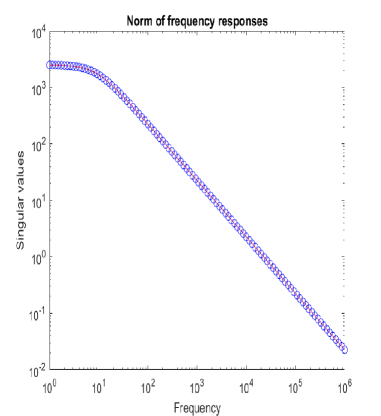
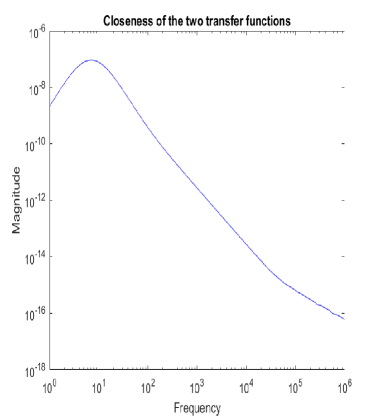
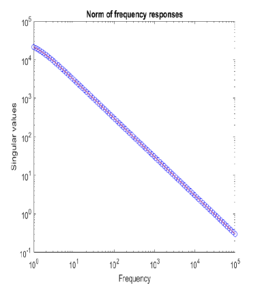
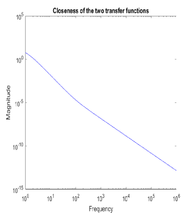
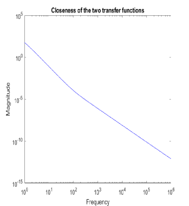
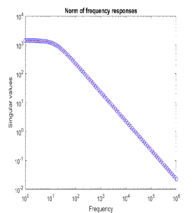
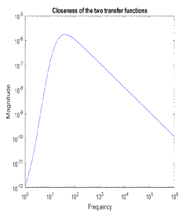
The performance of the methods is shown in the plots of Figs. 14, which report the frequency response of the original system (circles plot) compared to the frequency response of its approximation (solid plot). The right plots of these figures represent the exact error $\|\mathcal{F}(j\omega)-\mathcal{F}_{m}(j\omega)\|_{2}$ for different frequencies and different small space dimension.

Refer to caption
Refer to caption
Fig. 1: Example 1.1. Left: $\|{\mathcal{F}(j\omega)}\|_{2}$ and it’s approximation $\|\mathcal{F}_{m}(j\omega)\|_{2}$. Right: the exact error $\|\mathcal{F}(j\omega)-\mathcal{F}_{m}(j\omega)\|_{2}$ using the TRBA algorithm with $m=5$.
Refer to caption
Refer to caption
Fig. 2: Example 1.1. Left: $\|{H(j\omega)}\|_{2}$ and it’s approximation $\|H_{m}(j\omega)\|_{2}$. Right: the exact error $\|H(j\omega)-H_{m}(j\omega)\|_{2}$ using the TRBL algorithm with $m=10$.
Refer to caption
Refer to caption
Fig. 3: Example 1.2. Left: $\|{H(j\omega)}\|_{2}$ and it’s approximation $\|H_{m}(j\omega)\|_{2}$. Right: the exact error $\|H(j\omega)-H_{m}(j\omega)\|_{2}$ using the TRBA algorithm with $m=10$.
Refer to caption
Refer to caption
Fig. 4: Example 1.2. Left: $\|{\mathcal{F}(j\omega)}\|_{2}$ and it’s approximation $\|\mathcal{F}_{m}(j\omega)\|_{2}$. Right: the exact error $\|\mathcal{F}(j\omega)-\mathcal{F}_{m}(j\omega)\|_{2}$ using the TRBL algorithm with $m=15$.

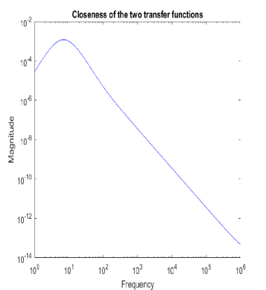
Example 2. For this experiment, we show the results obtained from the tensor Balanced Truncation method explained in Section 5, to reduce the order of MLTI systems. The following data were used:

$\bullet$ The tensor $\mathcal{A}\in\mathbb{R}^{N\times N\times N\times N}$, with N = 100, is constructed from a tensorization of a triangular matrix $A\in\mathbb{R}^{NN\times NN}$ constructed using the MATLAB function spdiags.

$\bullet\mathcal{B},\mathcal{C}^{T}\in\mathbb{R}^{N\times N\times K_{1}\times K_{2}}$ are chosen to be random tensors with $K_{1}=K_{2}=3$.

$\bullet$ We use Algorithm 3 to solve the two continuous Lyapunov equations (38) by setting
m = 30 (i.e., the maximum number of iterations) and the tolerance $\epsilon=10^{-8}$.

The frequency response (solid plot) of this test example is given in the left of Fig. 7.5 and is compared to the frequency responses of the 5 order approximation (circles plot). The exact error $\|\mathcal{F}(j\omega)-\mathcal{F}_{m}(j\omega)\|_{2}$ produced by this process is shown in the right of Fig. 5.

Refer to caption
Refer to caption
Fig. 5: Left: $\|{\mathcal{F}(j\omega)}\|_{2}$ and it’s approximation $\|\mathcal{F}_{m}(j\omega)\|_{2}$. Right: the exact error $\|\mathcal{F}(j\omega)-\mathcal{F}_{m}(j\omega)\|_{2}$ for m=5.

Example 3. For the last experiment, we compared the performance of the tensor classical block Lanczos (TCBL) and the tensor rational block Lanczos (TRBL) algorithms when applied to solve high order continuous-time Lyapunov tensor equations. The following data were used:

$\bullet$ The tensor $\mathcal{A}\in\mathbb{R}^{N\times N\times N\times N}$ is constructed from a tensorization of a triangular matrix $A\in\mathbb{R}^{NN\times NN}$ constructed using the MATLAB function spdiags.

$\bullet\mathcal{B},\mathcal{C}^{T}\in\mathbb{R}^{N\times N\times K_{1}\times K_{2}}$ are chosen to be random tensors.

$\bullet$ We use Algorithm 3 to solve the two continuous Lyapunov equations (38) by setting m = 30 (i.e., the maximum number of iterations) and the tolerance $\epsilon=10^{-8}$.

As observed from Table 2, TRBL process is more effective than the TCBL process, and the number of iterations required for convergence is small. However, the TCBL algorithm performs better in terms of computation time.

Table 2: Results obtained from the two methods for solving high order coupled Lyapunov tensor equations.
$(N,K_{1},K_{2})$    Algorithm    Iter    Res    time (s)
(80,3,3) TCBL 11 $4.02\times 10^{-9}$ 15.42
TRBL 6 $9.71\times 10^{-10}$ 138.24
(80,3,4) TCBL 11 $4.52\times 10^{-9}$ 18.80
TRBL 6 $8.28\times 10^{-10}$ 142.5
(100,3,3) TCBL 12 $3.96\times 10^{-9}$ 40
TRBL 7 $8.07\times 10^{-9}$ 206.14
(100,3,4) TCBL 11 $2.23\times 10^{-8}$ 47.85
TRBL 7 $4.28\times 10^{-9}$ 403.37

8 Conclusion

In this paper, we introduce the tensor rational block Krylov subspace methods based on Arnoldi and Lanczos algorithms. We extended the application of these methods to reduce the order of multidimensional linear time-invariant (MLTI) systems and to solve continuous-time Lyapunov tensor equations. Moreover, we derived some theoretical results concerning the error estimations between the original and the reduced transfer functions and the residual of continuous-time Lyapunov tensor equations. We presented an adaptive approach for choosing the interpolation points used to construct the tensor rational Krylov subspaces. Finally, numerical results are given to confirm the effectiveness of the proposed methods.

References

  • [1] O. ABIDI, M. HACHED AND K. JBILOU, Adaptive rational block Arnoldi methods for model reductions in large-scale MIMO dynamical systems, New Trend. Math., 4 (2016) 227-239.
  • [2] A. C. Antoulas, D. C. Sorensen, and S. Gugercin, A survey of model reduction methods for large scale systems, Contemp. Math., 280, 193-219 (2001).
  • [3] Z. Bai, D. Day, and Q. Ye, ABLE: An adaptive block Lanczos method for non-Hermitian eigenvalue problems, SIAM J. Matrix Anal. Appl., 20, 1060-1082 (1999).
  • [4] H. Barkouki, A. H. Bentbib and K. Jbilou, An adaptive rational block Lanczos-type algorithm for model reduction of large scale dynamical systems, J. Sci. Comput., 67, 221–236 (2016)
  • [5] A. Barraud, A numerical algorithm to solve atxa- x = q, IEEE Transac. Auto. Contr., 22 (1977), pp. 883–885
  • [6] M. J. Brazell, N. LI, C. Navasca, and C. Tamon, Solving multilinear systems via tensor inversion, SIAM J. Matrix Ana. Appl., 34 (2013), pp. 542–570.
  • [7] C. Chen, A. Surana, A. Bloch, and I. Rajapakse, Multilinear time invariant system theory, In 2019 Proceedings of the Conference on Control and its Applications, SIAM, (2019), pp. 118–125.
  • [8] C. Chen, Data-driven model reduction for multilinear control systems via tensor trains, submitted, https://arxiv.org/pdf/1912.03569.pdf, (2020)
  • [9] C. Chen, A. Surana, A. Bloch, and I. Rajapakse, Multilinear time invariant system theory, SIAM J. Contr. Optim.,, 59(1) (2021), pp. 749–776.
  • [10] M. El Guide, A. El Ichi, K. Jbilou and F. P. A. Beik, Tensor Krylov subspace methods via the Einstein product with applications to image and video processing, App. Numer. Math., 181 (2022), 347-363.
  • [11] K. Gallivan, E. Grimme, and P. Van Dooren, Padé Approximation of Large-Scale Dynamic Systems with Lanczos Methods, in Proceedings of the 33rd IEEE Conference on Decision and Control, 443-448 1994.
  • [12] K. Gallivan, E. Grimme, and P. Van Dooren, A rational Lanczos algorithm for model reduction, Num. Alg., 12, 33-63 (1996).
  • [13] S. Gugercin and A. C. Antoulas, A survey of model reduction by balanced truncation and some new results, Internat. J. Control, 77(8) (2003), pp. 748–766.
  • [14] S. Gugercin, and A. C. Antoulas, Model reduction of large scale systems by least squares, Lin. Alg. Appl., 415(2-3), 290-321 (2006).
  • [15] K. Glover, All optimal Hankel-norm approximation of linear multivariable systems and their $L^{\infty}$-error bounds, Int. J. Contr., 39 (6), 1115-1193 (1984).
  • [16] G. H. Golub and C. F. Van Loan, Matrix Computations. Johns Hopkins University Press., Baltimore, (1996).
  • [17] E. Grimme, Krylov Projection Methods for Model Reduction, PhD thesis, ECE Dept., University of Illinois, Urbana-Champaign, 1997.
  • [18] E. Grimme, K. Gallivan, and P. Van Dooren, Rational Lanczos algorithm for model reduction II: Interpolation point selection, Technical report, University of Illinois at Urbana Champaign, 1998.
  • [19] M.A. HAMADI, K. JBILOU , AND A. RATNANI, A model reduction method for large-scale linear multidimensional dynamical systems, submitted, https://arxiv.org/abs/2305.09361.
  • [20] M. Heyouni, K. Jbilou, A. Messaoudi, and K. Tabaa, Model reduction in large scale MIMO dynamical systems via the block Lanczos method, Comp. Appl. Math., 27(2), 211-236 (2008).
  • [21] M. Heyouni and K. Jbilou, An extended block arnoldi method for large matrix riccati equations, Elect. Trans. Numer. Anal., 33 (2009), pp. 53–62.
  • [22] R.A. Horn and C.R. Johnson, Topics in Matrix Analysis. Cambridge University Press, Cambridge, (1991).
  • [23] M. Frangos, and I. M. Jaimoukha, Adaptive rational Krylov algorithms for model reduction, In Proc. European Control Conference, 4179-4186 (2007).
  • [24] M. Frangos, and I. M. Jaimoukha, Adaptive rational interpolation: Arnoldi and Lanczos-like equations, European Journal of Control, 14(4), 342-354 (2008).
  • [25] T. G. Kolda and B. W. Bader, Tensor decompositions and applications, SIAM review, 51 (2009), pp. 455–500.
  • [26] H. J. Lee, C. C. Chu, and W. S. Feng, An adaptive-order rational Arnoldi method for model-order reductions of linear time-invariant systems, Linear Algebra Appl., 415, 235-261 (2006).
  • [27] M. Liang and B. Zheng, Further results on Moore–Penrose inverses of tensors with application to tensor nearness problems, Computers and Math. with App., 77(5) (2019), 0898-1221.
  • [28] C. B. Lizhu Sun, Baodong Zheng and Y. Wei, Moore–penrose inverse of tensors via einstein product, Linear and Multilinear Algebra, 64 (2016), pp. 686–698.
  • [29] V. Mehrmann and T. Stykel, Balanced truncation model reduction for large-scale systems in descriptor form, Lecture Notes in Computational Science and Engineering, 45 (2005), pp. 83–115.
  • [30] B. C. Moore, Principal component analysis in linear systems: controllability, observability and model reduction, IEEE Trans. Auto. Cont., AC-26 (1981), pp. 17–32.
  • [31] M. Nip, J. P. Hespanha, and M. Khammash, Direct numerical solution of algebraic lyapunov equations for large-scale systems using quantized, in 2013 52nd IEEE Conference on Decision and Control (CDC), (2013), pp. 1950–1957.
  • [32] M. Rogers, L. Li and S. J. Russell, Multilinear Dynamical Systems for Tensor Time Series, Part of Advances in Neural Information Processing Systems 26, (2013).
  • [33] V. Simoncini, D. B. Szyld, and M. Marlliny, On two numerical methods for the solution oflarge-scale algebraic riccati equations, IMA Journal of Numerical Analysis, 34 (2014), pp. 904–920.
  • [34] W. Yuchao and W. Yimin, Generalized eigenvalue for even order tensors via Einstein product and its applications in multilinear control systems, Comput. Appl. Math., 41(8) (2022).