The zero entropy locus for the Lozi maps

Abstract.

We study the zero entropy locus for the Lozi maps. We first define a region $R$ in the parameter space and prove that for the parameters in $R$, the Lozi maps have the topological entropy zero. $R$ is contained in a larger region where every Lozi map has a unique period-two orbit, and that orbit is attracting. It is easy to see that the zero entropy locus cannot coincide with that larger region, since it contains parameters for which the fixed point of the corresponding Lozi map has homoclinic points.

2020 Mathematics Subject Classification: 37B40, 37E30, 37B25

Key words and phrases: Lozi map, topological entropy, zero entropy.

1. Introduction

In 1978 Lozi constructed a two parameter family $L_{a,b}(x,y)=(1+y-a|x|,bx)$ of piecewise affine homeomorphisms of the Euclidean plane to itself, for which he provided numerical evidence that for parameters value $a=1.7$ and $b=0.5$ the map has strange attractor (see [1]). In 1980 the first author of this paper proved that for a large set of parameters, the Lozi maps have indeed hyperbolic strange attractors (see [2]). Although in the last forty five years many results about the Lozi maps and their attractors have been obtained, many important questions have stayed unanswered yet. It is still not known how topological entropy and periodic points depend on parameters, whether there are parameters for which distinct Lozi maps are topologically conjugate, or their attractors are homeomorphic, to mention just a few well-known open problems.

One of those open problems, related to all the above mentioned, is to find the set of parameters for which the Lozi maps have zero entropy.

In [3] Yildiz proved that the topological entropy of the Lozi map $L_{a,b}$ is zero, $h_{top}(L_{a,b})=0$, in the following three regions of the parameter space:

1. $0<|b|\leq 1$ and $a\leq b-1$

   In that region $L_{a,b}$ does not have fixed or periodic points.

2. $0<b<1$ and $b-1<a\leq 1-b$

   In that region, and if $a<1-b$, $L_{a,b}$ has a unique attracting fixed point $X=(\frac{1}{1+a-b},\frac{b}{1+a-b})$ in the first quadrant, and does not have other periodic points. If $a=1-b$, $L_{a,b}$ has the fixed point $X$, which is not hyperbolic, and it is the midpoint of a line segment $I$ of period-two points, where $I=\{(x,y)\in{\mathbb{R}}^{2}:bx+y=\frac{b}{1-b},\ 0\leq x\leq\frac{1}{1-b}\}$.

3. In a small neighborhood $U$ of the point $(a,b)=(1,0.5)$.

In this paper, we improve the zero entropy result obtained by Yildiz.

In the next section we first define a region in the parameter space that we denote by $R$, see Figure 1.

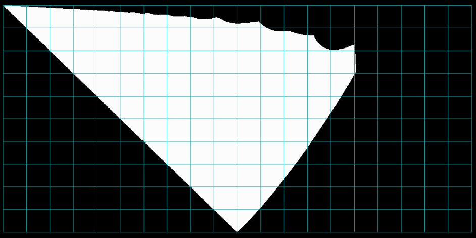
Figure 1. The parameter $a$ is on the horizontal axis and goes from 0 to 2. The parameter $b$ is on the vertical axis and goes from 0 to 1. The region $R$ is in white.

Then we prove the following theorem:

Theorem 1.1.

For $(a,b)\in R$, $h_{top}(L_{a,b})=0$.

After that we describe rigorously the region $R$ and show that it looks as in Figure 1.

In Section 3 we present a few numerical results that inspired our conjecture that the topological entropy of the Lozi map $L_{a,b}$ is zero if $L_{a,b}$ has a unique period-two orbit that is attracting and the fixed point $X$ does not have homoclinic points.

2. The zero entropy locus

Let us consider the following region in the parameter space: $0<b<1$ and $1-b<a<1+b$. In that region $L_{a,b}$ has two saddle fixed points, $X=(\frac{1}{1+a-b},\frac{b}{1+a-b})$ in the first quadrant and $Y=(\frac{1}{1-a-b},\frac{b}{1-a-b})$ in the third quadrant. The eigenvalues of $DL_{a,b}$ (the derivative of $L_{a,b}$) are

$$\lambda^{u}_{X}=(-a-\sqrt{a^{2}+4b})/2\ \textrm{ and }\ \lambda_{X}^{s}=(-a+\sqrt{a^{2}+4b})/2\ \textrm{ at }\ X$$

and

$$\lambda_{Y}^{u}=(a+\sqrt{a^{2}+4b})/2\ \textrm{ and }\ \lambda_{Y}^{s}=(a-\sqrt{a^{2}+4b})/2\ \textrm{ at }\ Y.$$

The eigenvector corresponding to an eigenvalue $\lambda$ is $\lambda\choose b$.

From now on, for a point $P\in\mathbb{R}^{2}$, let $P^{n}=L_{a,b}^{n}(P)$, $n\in{\mathbb{Z}}$, where $P^{0}=P$. One half of the unstable manifold $W^{u}_{X}$ of $X$, starts from $X$ and goes to the right, we denote it by $W^{u+}_{X}$. It intersects the horizontal axis for the first time at the point

$$Z=\left(\frac{2+a+\sqrt{a^{2}+4b}}{2(1+a-b)},0\right).$$

The other half, that starts at $X$ and goes to the left, we denote by $W^{u-}_{X}$. It intersect the $y$-axis for the first time at the point $Z^{-1}$. Note that $Z^{2n}\in W^{u+}_{X}$ and $Z^{2n-1}\in W^{u-}_{X}$ for every $n\in{\mathbb{N}}_{0}$.

Also, there are two attracting period-two points, $P^{\prime}$ in the second quadrant and $P$ in the fourth quadrant,

$$P^{\prime}=\left(\frac{1-a-b}{a^{2}+(1-b)^{2}},\frac{b(1+a-b)}{a^{2}+(1-b)^{2}}\right),\ P=\left(\frac{1+a-b}{a^{2}+(1-b)^{2}},\frac{b(1-a-b)}{a^{2}+(1-b)^{2}}\right),$$

and there are no other period-two points. Also, for $a=1+b$, $P^{\prime}$ and $P$ are not hyperbolic, but for $a>1+b$, they are hyperbolic saddle points.

Note that it is enough to consider the Lozi maps with $|b|\leq 1$ since the maps with $|b|>1$ are, up to an affine conjugacy, inverses of the maps with $|b|<1$.

From now on let $R$ denote the region in the parameter space such that $0<b<1$, $1-b<a<1+b$ and for every $k\in{\mathbb{N}}_{0}$, $Z^{2k-1}$ belongs to the left half-plane and $Z^{2k}$ belongs to the right half-plane.

Proof of Theorem 1.1.

Let $(a,b)\in R$. We want to prove that $h_{top}(L_{a,b})=0$. Let $ZL:=\{L_{a,b}^{2k-1}(Z):k\in{\mathbb{N}}_{0}\}$ and $ZR:=\{L_{a,b}^{2k}(Z):k\in{\mathbb{N}}_{0}\}=L_{a,b}(ZL)$. Let us consider their convex hulls $\mathop{\mathrm{missing}}{Conv}(ZL)$ and $\mathop{\mathrm{missing}}{Conv}(ZR)$. Since $L_{a,b}$ maps the left half-plane to the lower half-plane, and the right half-plane to the upper one, $\mathop{\mathrm{missing}}{Conv}(ZL)$ is contained in the second quadrant and $\mathop{\mathrm{missing}}{Conv}(ZR)$ is contained in the fourth quadrant. Also $L_{a,b}(\mathop{\mathrm{missing}}{Conv}(ZL))=\mathop{\mathrm{missing}}{Conv}(ZR)$ and $L_{a,b}(\mathop{\mathrm{missing}}{Conv}(ZR))\subset\mathop{\mathrm{missing}}{Conv}(ZL)$. In both sets, $\mathop{\mathrm{missing}}{Conv}(ZL)$ and $\mathop{\mathrm{missing}}{Conv}(ZR)$, the map is globally linear, so their union is attracted to the periodic orbit $\{P^{\prime},P\}$. This in particular means that $W^{u}(X)\cup\{P^{\prime},P\}$ is compact, connected and invariant.

Let us denote by $W^{s+}_{X}$ the upper connected component of the stable manifold of $X$ which starts at $X$ and goes up, and by $W^{u+}_{Y}$ the lower connected component of the unstable manifold of the other fixed point $Y$ in the third quadrant which starts at $Y$ and goes down. Let us denote by $M$ the union of $W^{u}_{X}$, $P^{\prime}$, $P$, $W^{s+}_{X}$, $W^{u+}_{Y}$ and $\infty$, $M=W^{u}_{X}\cup\{P^{\prime},P\}\cup W^{s+}_{X}\cup W^{u+}_{Y}\cup\{\infty\}$. Then $M$ is invariant, compact, connected in the extended plane and does not separate the extended plane, nor the plane.

Let us denote by $U$ the complement of $M$ in the plane (that is, $U={\mathbb{R}}^{2}\smallsetminus M$). Then $U$ is invariant by construction and does not contain any fixed point of $L_{a,b}^{2}$. Also, $U$ is open and simply connected in the plane and therefore homeomorphic to the open unit disc, and moreover to the plane. The Brouwer plane translation theorem (BPTT) says that if $h$ is an orientation preserving homeomorphism of the plane which is fixed point free, then every point of the plane is contained in a properly embedded line $l$ such that $l$ does not intersect $h(l)$, and $l$ is separating $h(l)$ from $h^{-1}(l)$. In our case, $L_{a,b}^{2}|_{U}$ satisfies assumptions of BPTT and therefore every point of $U$ is a wandering point for $L_{a,b}^{2}$. This means that the non-wandering set of $L_{a,b}^{2}$ consists only of the fixed points of $L_{a,b}^{2}$, and hence $h_{top}(L_{a,b}^{2})=2h_{top}(L_{a,b})=0$. ∎

Now, we will describe rigorously the region $R$ and show that it looks as in Figure 1. First, we will prove that there is a simply connected neighborhood of $(0,1)$ contained in $R$.

Note that for $(a,b)\in R$ and every $k\in{\mathbb{N}}_{0}$, $DL^{2}_{a,b}(Z^{2k})=DL^{2}_{a,b}(P)$ and its eigenvalues are $(-a^{2}+2b\pm a\sqrt{a^{2}-4b})/2$. Therefore, when $4b>a^{2}$, the part of the unstable manifold of $X$ which belongs to the fourth quadrant spirals towards $P$, and the part which belongs to the second quadrant spirals to $P^{\prime}$. In the next lemma, we will describe that behavior more precisely.

We will work with parameters $a,b$, where $b=1-ta$, $0<t<1$ and $a$ is close to $0$ (so $b$ is close to $1$). When we take limits as $a\to 0$, we will fix $t$ and treat $b$ as a function of $a$. We identify ${\mathbb{R}}^{2}$ with $\mathbb{C}$, and use both notations (even within the same formula).

The derivative of the second iterate of the Lozi map at the periodic point $P$ of period 2, which is in the fourth quadrant, is

$$A=\begin{pmatrix}b-a^{2}&a\\ -ab&b\end{pmatrix}=\begin{pmatrix}1-ta-a^{2}&a\\ -a+ta^{2}&1-ta\end{pmatrix}.$$

Lemma 2.1.

Let $v\in\mathbb{C}={\mathbb{R}}^{2}$. Then, as $a\to 0$, the broken line joining consecutive points $A^{n}v$ converges to the logarithmic spiral $\varphi\mapsto ve^{-t\varphi}e^{-i\varphi}$ locally uniformly in $t$.

Proof.

Let us define the matrix

$$B=\begin{pmatrix}b\cos a&b\sin a\\ -b\sin a&b\cos a\end{pmatrix}.$$

Then

$$\lim_{a\to 0}\frac{A-B}{a^{2}}=\begin{pmatrix}-1/2&t\\ 0&1/2\end{pmatrix}.$$

Moreover, for a given $\tau$, $0<\tau<1$, there exist $\varepsilon>0$, $\alpha>0$ and a constant $K:=K_{\alpha,\varepsilon}$ such that if $\tau-\varepsilon<t<\tau+\varepsilon$ and $a<\alpha$, then $\|A-B\|<Ka^{2}<ta$. Since $\|B\|=b$, we have always $\|B\|<1$ and $\|A\|\leq\|B\|+\|A-B\|<1-ta+Ka^{2}<1$.

We have

$$A^{n}-B^{n}=(A^{n}-BA^{n-1})+(BA^{n-1}-B^{2}A^{n-2})+\dots+(B^{n-1}A-B^{n}),$$

so for $\tau-\varepsilon<t<\tau+\varepsilon$ and $a<\alpha$

$$\begin{split}\|A^{n}-B^{n}\|&\leq\|A^{n}-BA^{n-1}\|+\|BA^{n-1}-B^{2}A^{n-2}\|+\dots+\|B^{n-1}A-B^{n}\|\\ &\leq\|A-B\|\big{(}\|A\|^{n-1}+\|B\|\cdot\|A\|^{n-2}+\dots+\|B\|^{n-1}\big{)}\leq n\|A-B\|.\end{split}$$

If $n\leq\varphi/a$ for some constant $\varphi$, we get $\|A^{n}-B^{n}\|\leq\varphi Ka$.

The action of the matrix $B$ is the same as the multiplication by $be^{-ai}$. Therefore, for $\tau-\varepsilon<t<\tau+\varepsilon$ and $a<\alpha$, we have for any $v\in{\mathbb{R}}^{2}=\mathbb{C}$ and $n=\lfloor\frac{\varphi}{a}\rfloor$

$$|A^{n}v-vb^{n}e^{-ina}|\leq\varphi Ka|v|.$$

As $a\to 0$ (and $\tau-\varepsilon<t<\tau+\varepsilon$, $n=\lfloor\frac{\varphi}{a}\rfloor$), we get

$$\lim_{a\to 0}b^{n}e^{-ina}=\lim_{a\to 0}(1-ta)^{n}e^{-i\varphi}=\lim_{n\to\infty}\left(1-\frac{t\varphi}{n}\right)^{n}e^{-i\varphi}=e^{-t\varphi}e^{-i\varphi}.$$

Therefore, as $a\to 0$, the broken line joining consecutive points $A^{n}v$ converges to the logarithmic spiral $\varphi\mapsto ve^{-t\varphi}e^{-i\varphi}$ locally uniformly in $t$. ∎

Theorem 2.2.

Let $t_{0}$ be the root of the equation

(1) $$\sqrt{2}e^{-\frac{7}{4}\pi t}=1+t$$

($t_{0}\approx 0.0535502597736068$). There exists a lower semi-continuous function $a(t)$ such that if $t_{0}<t<1$, then for $a<a(t)$ (and $b=1-ta$) all even images of the point $Z$ are in the fourth quadrant, and all odd images of $Z$ are in the second quadrant. As a consequence, the unstable manifold $W^{u}_{X}$ of the fixed point $X$ is attracted to the periodic orbit $\{P,P^{\prime}\}$ of period $2$ and $\mathop{\mathrm{missing}}{Cl}W^{u}_{X}=W^{u}_{X}\cup\{P,P^{\prime}\}$.

Proof.

Fix $t<1$. Let us consider the spiral described in Lemma 2.1, with center at $P$ and starting at $Z$. Note that the points $P$ and $Z$ (as well as $X$, $P^{\prime}$, $Z^{k}$, $k\in{\mathbb{N}}$) go to infinity as $a$ approaches zero. For that reason we will scale these points by the factor $a$. In this case the scaled points converge when $a$ goes to zero, as we will see below. Moreover, the below statements about spirals hold if and only if the analogous statements hold for the scaled points.

The points $P$ and $Z$, scaled by the factor $a$, have the following forms:

$$aP=\left(\frac{1+t}{1+t^{2}},\ \frac{(1-ta)(t-1)}{1+t^{2}}\right),\ aZ=\left(\frac{2+a+\sqrt{a^{2}+4-4ta}}{2(1+t)},\ 0\right).$$

The slope of the segment between $Z$ and $Z^{1}$, that is the part of the unstable manifold of $X$ which contains $X$, is $(-a-\sqrt{a^{2}+4b})/2=(-a-\sqrt{a^{2}+4-4ta})/2$, so it converges to $-1$ when $a$ goes to $0$. Also, as $a$ goes to zero, the linear maps defining our Lozi map on two half-planes go to the same limit. Therefore, the angle between the segments $[Z^{1},Z]$ and $[Z,Z^{2}]$, as well as between the segments $[aZ^{1},aZ]$ and $[aZ,aZ^{2}]$, goes to zero. Hence, in the limit the tangent to our spiral at $aZ$ has slope $-1$.

First, we will show that if $t=t_{0}$ then the spiral is tangent to the $x$-axis. Thus, if $t>t_{0}$, it does not intersect the $x$-axis. Similarly, if $t=t_{1}$, where $t_{1}$ is the root of the equation

(2) $$\sqrt{2}e^{-\frac{5\pi}{4}t}=\frac{(1+t)^{2}}{1-t},$$

then the spiral is tangent to the $y$-axis, so if $t>t_{1}$, it does not intersect the $y$-axis. However, $t_{1}<t_{0}$, so if $t>t_{0}$ then our spiral does not intersect any of the coordinate axes.

Now we will make calculations in $\mathbb{C}$. Set

$$p=\lim_{a\to 0}aP=\frac{t+1}{t^{2}+1}+i\frac{t-1}{t^{2}+1},\ \ \ \ \ z=\lim_{a\to 0}aZ=\frac{2}{t+1}.$$

To get the tangent line to the spiral to change from slope $-1$ to slope $0$ (above $p$), we have to go along the spiral by the angle $\frac{7}{4}\pi$. This means that $t_{0}$ is the root of the equation

(3) $$\operatorname{Im}\left(p+(z-p)e^{-t\frac{7}{4}\pi}e^{-i\frac{7}{4}\pi}\right)=0.$$

Similarly, $t_{1}$ is the root of the equation

(4) $$\operatorname{Re}\left(p+(z-p)e^{-t\frac{5}{4}\pi}e^{-i\frac{5}{4}\pi}\right)=0.$$

Equation (3) can be rewritten as

$$\operatorname{Im}\left((z-p)e^{-i\frac{7}{4}\pi}\right)=-\operatorname{Im}(p)e^{t\frac{7}{4}\pi}.$$

We have

$$z-p=\frac{(t-1)^{2}}{(t+1)(t^{2}+1)}-i\frac{t-1}{t^{2}+1},$$

so

$$\frac{z-p}{\operatorname{Im}(p)}=\frac{t-1}{t+1}-i.$$

Moreover, $e^{-i\frac{7}{4}\pi}=\frac{\sqrt{2}}{2}(1+i)$. Therefore, (3) becomes

$$\frac{\sqrt{2}}{2}\operatorname{Im}\left(\left(\frac{t-1}{t+1}-i\right)(1+i)\right)=-e^{t\frac{7}{4}\pi},$$

which is equivalent to (1).

Similar calculations show that (4) is equivalent to (2). The solution is approximately $t_{1}\approx 0.05019615992097643$, so $t_{1}<t_{0}$.

Fix $\tau,\ t_{0}<\tau<1$. As we have already showed, our spiral (with center at $P$ and starting at $Z$) does not intersect the coordinate axes (except at the initial point $Z$). By Lemma 2.1, there exist $\alpha>0$ and $\varepsilon>0$ such that for $a<\alpha$ and $\tau-\varepsilon<t<\tau+\varepsilon$, the broken line joining the consecutive even images of the point $Z$ is so close to the spiral that all even images of the point $Z$ are in the fourth quadrant. Let us denote by $S(\tau)$ the set of all such $\alpha$ for which there exists $\varepsilon>0$ that satisfies the above property. We define $a(\tau)=\sup S(\tau)$. Recall that the function $f$ is called lower semi-continuous at $x_{0}$ if for every $y<f(x_{0})$ there exists a neighborhood $U$ of $x_{0}$ such that $f(x)>y$ for all $x\in U$. Clearly, the map $\tau\mapsto a(\tau)$ is lower semi-continuous and if $t_{0}<\tau<1$, then for $a<a(\tau)$ (and $b=1-\tau a$) all even images of the point $Z$ are in the fourth quadrant. Consequently, all odd images of $Z$ are in the second quadrant, the unstable manifold $W^{u}_{X}$ of the fixed point $X$ (which then consists of a segment in the first quadrant, joins consecutive even images of $Z$ in the fourth quadrant and joins consecutive odd images of $Z$ in the second quadrant) is attracted to the periodic orbit $\{P,P^{\prime}\}$ of period $2$ and $\mathop{\mathrm{missing}}{Cl}W^{u}_{X}=W^{u}_{X}\cup\{P,P^{\prime}\}$. ∎

Figure 2 shows the stable and unstable manifolds of the fixed point $X$ for the parameters $a=0.05$ and $b=0.997$.

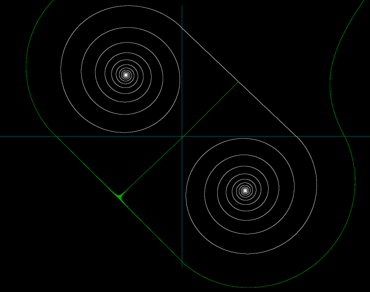
Figure 2. $a=0.05$ and $b=0.997$. The unstable manifold is in white (the spiral) and the stable manifold is in green (the curve that intersects the spiral in one point).

Since the boundary of the region $R$ is a result of intersections of the coordinate axes and the unstable manifold of $X$ which is piecewise linear, the boundary of $R$ is piecewise algebraic. The boundary curves are given by the following conditions: Let $x_{n}$ and $y_{n}$ denote the $x$- and $y$-coordinate of $Z^{n}$, that is, $Z^{n}=(x_{n},y_{n})$, $n\in{\mathbb{N}}$. First recall that $Z$ belongs to the right half-plane and $Z^{1}$ belongs to the left half-plane for every $0<b<1$ and $a>1-b$. Let us denote by $C_{n}$, $n\geq 2$, the curve in the parameter space such that $Z^{2k}$ belongs to the right half-plane for $2k<n$, $Z^{2k+1}$ belongs to the left half-plane for $2k+1<n$, and $Z^{n}\in y$-axis. Then

$$C_{2}=\{(a,b):0\leq b\leq 1,\ 1-b\leq a\leq 1+b,\ x_{2}=0\},$$

and for every $k\in{\mathbb{N}}$,

$$C_{2k+1}=\{(a,b):0\leq b\leq 1,\ 1-b\leq a\leq 1+b,\ x_{2j-1}\leq 0,\ x_{2j}\geq 0,\ j=1,\dots k,\ x_{2k+1}=0\},$$

$$C_{2k+2}=\{(a,b):0\leq b\leq 1,\ 1-b\leq a\leq 1+b,\ x_{2j}\geq 0,\ x_{2j+1}\leq 0,\ j=1,\dots k-1,\ x_{2k+2}=0\}.$$

Example 2.3.

By direct calculation one can get the following equations of $C_{2}$, $C_{3}$, $C_{4}$ and $C_{5}$.

1. $b^{2}+(-2a^{2}+a+1)b-2a^{3}+a^{2}+3a+1=0$

2. $b^{2}-(4a^{2}-2)b+2a^{4}-3a^{2}+1=0$ (only the right branch is important) and $b+a-1=0$

3. $b^{4}-(8a^{2}-a-1)b^{3}-(-8a^{4}+8a^{3}+a^{2}-2a-1)b^{2}-(2a^{6}-8a^{5}+4a^{4}+9a^{3}-3a^{2}-6a-1)b-2a^{7}+2a^{6}+4a^{5}-3a^{4}-5a^{3}+a^{2}+3a+1=0$ (only the upper branch is important)

4. $b^{4}-(12a^{2}-2)b^{3}-(-22a^{4}+15a^{2}-3)b^{2}-(12a^{6}-16a^{4}+12a^{2}-2)b+2a^{8}-4a^{6}+5a^{4}-3a^{2}-1=0$ (only the upper branch is important)

Figure 3. $C_{2}$ is black, $C_{3}$ is blue, $C_{4}$ is green and $C_{5}$ is red.

Lemma 2.4.

For $k\geq 4$, let $(a_{k},b_{k})=\min C_{k}$. Then $b_{k+2}\geq b_{k}$ and $a_{k+2}\leq a_{k}$. Moreover, $\lim_{k\to\infty}(a_{k},b_{k})=(0,1)$.

Proof.

Recall that for $b>a^{2}/4$, the eigenvalues of $DL^{2}_{a,b}$ are $\lambda(a,b)=u\pm iv$, with $u=(2b-a^{2})/2$, $v=a\sqrt{4b-a^{2}}/2$, $|\lambda|=b$, and the argument of $\lambda$ is $\varphi=\varphi(a,b)=\arctan\frac{a\sqrt{4b-a^{2}}}{2b-a^{2}}$. By calculating the partial derivatives of $\varphi(a,b)$ with respect to $a$ and with respect to $b$, it is easy to see that: For $a$ fixed, the map $b\mapsto\varphi(a,b)$ is a decreasing function, and for $b$ fixed, the map $a\mapsto\varphi(a,b)$ is an increasing function.

First, we will prove by induction that $b_{2k+2}\geq b_{2k}$ and $a_{2k+2}\leq a_{2k}$ for every $k\geq 2$. By direct calculation we have that $b_{6}>b_{4}$ and $a_{6}<a_{4}$. For $(a_{6},b_{6})$ the point $Z^{6}$ belongs to the $y$-axis. In transition from that state to the state where $Z^{8}$ belongs to the $y$-axis while $Z^{2j}$ are in the right half-plane and $Z^{2j+1}$ are in the left half-plane, for $j=1,2,3$, the map $\varphi$ decreases, implying that $a$ decreases and $b$ increases. Therefore, $b_{8}\geq b_{6}$ and $a_{8}\leq a_{6}$.

Let us consider $(a_{2k},b_{2k})$. For that pair of parameters the point $Z^{2k}$ belongs to the $y$-axis. Now again, in transition from that state to the state where $Z^{2k+2}$ belongs to the $y$-axis, $Z^{2j}$ are in the right half-plane and $Z^{2j+1}$ are in the left half-plane, for $j=1,\dots,k$, the map $\varphi$ decreases, implying that $a$ decreases and $b$ increases. Therefore, $b_{2k+2}\geq b_{2k}$ and $a_{k+2}\leq a_{k}$.

In an analogous way we can get $b_{2k+3}\geq b_{2k+1}$ and $a_{2k+3}\leq a_{2k+1}$ for every $k\in{\mathbb{N}}$.

Note that in every move from $(a_{k},b_{k})$ to $(a_{k+2},b_{k+2}$) we can obtain that only finitely many iterates of $Z$ belong to the $y$-axis (at most two in the upper half-plane and two in the lower half-plane). Since the orbit of $Z$ is countable infinite, we have infinitely many different points $(a_{k},b_{k})$ and, by Theorem 2.2, $\lim_{k\to\infty}(a_{k},b_{k})=(0,1)$. ∎

Figure 4. The region obtained by 8 assumptions: $Z^{2}$, $Z^{4}$, $Z^{6}$ and $Z^{8}$ belong to the right half-plane and $Z^{3}$, $Z^{5}$, $Z^{7}$ and $Z^{9}$ belong to the left half-plane.

The next proposition gives scaling of the sequence $(a_{2k})_{k\in{\mathbb{N}}}$.

Proposition 2.5.

$\lim_{k\to\infty}2ka_{2k}=7\pi/4$.

Proof.

By lemma 2.1 we have that as $a\to 0$, the broken line joining consecutive points $Z^{2n}=A^{n}Z$, $n\in{\mathbb{N}}$, converges to the logarithmic spiral $\varphi\mapsto Ze^{-t\varphi}e^{-i\varphi}$ in the fourth quadrant which start at $Z$ and has center at $P$, with $n=\lfloor\frac{\varphi}{a}\rfloor$. Since we are interested in parameters $(a_{2k},b_{2k})$, $k\in{\mathbb{N}}$, $k\geq 2$, for which $Z^{2k}$ lies on the $y$-axis and $b_{2k}$ is minimal for that property, by Theorem 2.2 we have $\varphi=7\pi/4$. Therefore, $\lim_{k\to\infty}2ka_{2k}=7\pi/4$. ∎

Figure 5 shows a part of region $R$ obtained numerically (in white), but in coordinates $c$ (the horizontal axis) and $t$ (the vertical axis), where $c=1/a$ and $t=(1-b)/a$. With such a choice of coordinates, scaling of the sequence $((a_{k},b_{k}))_{k=4}^{\infty}$, where $(a_{k},b_{k})=\min C_{k}$, is easy to notice.

Figure 5. $c$ (the horizontal axis) goes from 24 to 26 and $t$ (the vertical axis) goes from 0.05355 to 0.0536.

3. Numerical results

Figure 6 shows two regions in the parameter space (the parameter $a$ is on the horizontal axis and the parameter $b$ is on the vertical axis). As before, the region $R$ is in white. The red region presents the set of parameters where not all odd iterates of $Z$ are in the second quadrant and not all even iterates of $Z$ are in the fourth quadrant, but still there are no homoclinic points of the fixed point $X$.

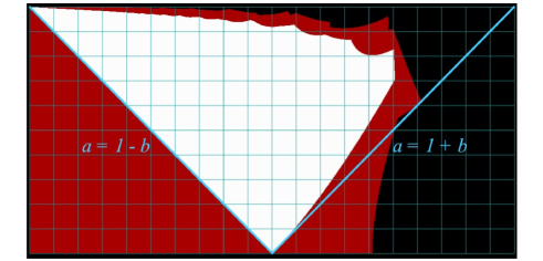
Figure 6. The figure shows several regions in the parameter space obtained numerically. The parameter $a$ is on the horizontal axis and goes from 0 to 2. The parameter $b$ is on the vertical axis and goes from 0 to 1. The region $R$ is in white. The red and white regions together present the set of parameters where there are no homoclinic points of the fixed point $X$. In the region $1-b<a<1+b$ the period-two points $P^{\prime}$ and $P$ are attracting. Note that for $a>1+b$ the period-two points $P^{\prime}$ and $P$ are saddle, so the Lozi map $L_{a,b}$ has heteroclinic points.

Figure 7 shows the stable and unstable manifolds of the fixed point $X$ for two different pairs of parameters, both from the red region (the stable manifold is in yellow and the unstable manifold is in white). Those pictures suggest that for the parameters in the red region the set $W^{u}(X)\cup\{P^{\prime},P\}$ might also be compact, connected and invariant, implying the zero entropy for the corresponding Lozi maps.

Figure 7. In both figures, the stable manifold is in yellow and the unstable manifold is in white. Left $a=1.16$, $b=0.95$; right $a=0.4$, $b=0.997$.

We conjecture that the topological entropy of the Lozi map is zero if the period-two orbit $\{P,P^{\prime}\}$ is attracting and the fixed point $X$ does not have homoclinic points, that is, for parameters $0<b<1$ and $1-b<a<1+b$ that are contained in the white and red regions of Figure 6.

The boundary of the red region consists of algebraic curves that are given by the existence of certain ‘tangential’ homoclinic points of $X$. Below we give equations of the first four curves that form the right-hand part of the boundary of the red region (see figure 8):

1. Curve $B_{1}$ is given by the equation

   $$a^{3}-4a+(a^{2}-2b)\sqrt{a^{2}+4b}=0.$$

   For $(a,b)\in B_{1}$ and $b\in[0,0.549134]$ the stable and unstable manifolds of $X$ intersect in $L^{2}(Z)$ ‘tangentially’: $L^{2}(Z)\in[K,V]\subset[X,V]\subset W^{s}_{X}$, where $K$ lies on the $x$-axis, $V$ lies on the $y$-axis and the interval $(K,V)$ does not intersect the coordinate axes.

2. Curve $B_{2}$ is given by the equation

   $2a^{6}+2a^{5}(1-2b)-11a^{4}b+a^{3}b(4b^{2}+6b-9)+3a^{2}b^{2}(2b+1)+4ab^{2}(b^{2}+b+1)+4b^{3}+(2a^{5}+2a^{4}(1-2b)-7a^{3}b+a^{2}b(4b^{2}+6b-5)+ab^{2}(2b+5)+2b^{2})\sqrt{a^{2}+4b}=0$.

   For $(a,b)\in B_{2}$ and $b\in[0.549134,0.602505]$ the stable and unstable manifolds of $X$ intersect ‘tangentially’ in $V$: $V\in[L^{2}(Z),T]\subset W^{u}_{X}$, where $T$ lies on the $x$-axis, $T\neq Z$, and the segment $[L^{2}(Z),T]$ intersects the $x$-axes only at the point $T$.

3. Curve $B_{3}$ is given by the equation

   $$a-b-1=0,\ \ b\in[0.602505,0.617056].$$

4. Curve $B_{4}$ is given by the equation

   $$a^{5}+2a^{3}(b-3)-6a^{2}-4a+4ab(b-1)+(a^{4}+2a^{2}+2a-2b^{2})\sqrt{a^{2}+4b}=0.$$

   For $(a,b)\in B_{4}$ and $b\in[0.617056,0.946803]$ the stable and unstable manifolds of $X$ intersect ‘tangentially’ in $L^{4}(Z)$: $L^{4}(Z)\in[K,V]$.

Figure 8. $B_{1}$ is green, $B_{2}$ is orange (only the lower branch is important), $B_{3}$ is blue and $B_{4}$ is yellow; the part of the boundary of the red region which is contained in the given curves is in black.

Michał Misiurewicz
Department of Mathematical Sciences
Indiana University Indianapolis
402 N. Blackford Street, Indianapolis, IN 46202
mmisiure@iu.edu
https://math.indianapolis.iu.edu/$\sim$mmisiure

Sonja Štimac
Department of Mathematics
Faculty of Science, University of Zagreb
Bijenička 30, 10 000 Zagreb, Croatia
sonja@math.hr
https://web.math.pmf.unizg.hr/$\sim$sonja/

References

[1]
R. Lozi, Un attracteur etrange(?) du type attracteur de
Hénon, J. Physique (Paris) 39 (Coll. C5) (1978), 9–10.
[2]
M. Misiurewicz, Strange attractor for the Lozi mappings,
Ann. New York Acad. Sci. 357 (1980) (Nonlinear Dynamics),
348–358.
[3]
I. B. Yildiz, Monotonicity of the Lozi family and the zero
entropy locus, Nonlinearity 24 (2011) 1613–1628.
[4] I. B. Yildiz, Discontinuity of Topological
Entropy for the Lozi Maps, Ergodic Theory and Dynamical Systems
32 (2012) 1783–1800.