BRST Noether Theorem and Corner Charge Bracket

Abstract

We provide a proof of the BRST Noether 1.5th theorem, conjectured in [JHEP 10 (2024) 055], for a broad class of rank-$1$ BV theories including supergravity and $2$-form gauge theories. The theorem asserts that the BRST Noether current of any BRST invariant gauge fixed Lagrangian decomposes on-shell into a sum of a BRST-exact term and a corner term that defines Noether charges. This extends the holographic consequences of Noether’s second theorem to gauge fixed theories and, in particular, offers a universal gauge independent Lagrangian derivation of the invariance of the $\mathcal{S}$-matrix under asymptotic symmetries. Furthermore, we show that these corner Noether charges are inherently non-integrable. To address this non-integrability, we introduce a novel charge bracket that accounts for potential symplectic flux and anomalies, providing an honest canonical representation of the asymptotic symmetry algebra. We also highlight a general origin of a BRST cocycle associated with asymptotic symmetries.

December 5, 2024

1 Introduction

More than a century ago, Emmy Noether discovered that classical gauge theories admit an infinite number of codimension two quantities $q_{\lambda}$, labeled by the local gauge parameter $\lambda(x)$ [1]. Since then, it has been understood that these quantities are the conserved charges associated with the gauge symmetry, supported on the corners of the Lorentzian spacetime manifold $M$. This result, known as Noether’s second theorem, has profound implications for holography, which have been extensively studied over the last decade (see [2] for an overview of the literature).

Notably, the Noether charges $q_{\lambda}$ associated with the invariance of a Lagrangian $L(\phi,\partial_{\mu}\phi)$ under gauge transformations $\delta_{\lambda}\phi=f(\phi)\lambda+f^{\mu}(\phi)\partial_{\mu}\lambda$ play a crucial role in defining asymptotic symmetries [3, 4, 5, 6, 7, 8]. The asymptotic symmetries or, in other words, the large gauge symmetries are defined as the gauge transformations parametrized by $\lambda(x)$ that preserve both the falloffs of the fields near the boundary $\varSigma=\partial M$ and the gauge fixing condition, and that lead to a non-vanishing Noether charge

$$Q_{\lambda}\equiv\int_{\partial\varSigma}q_{\lambda}\neq 0.$$ (1.1)

These large gauge symmetries generate non-trivial physical transformations on the phase space of the theory and are no longer gauge redundancies.

With the discovery of the infrared triangle [9, 10, 11, 12], it is now understood that asymptotic symmetries govern the infrared behavior of a given gauge theory, as they are equivalent to the soft theorem of the associated massless gauge particle [13, 14, 10, 12, 11]. To establish this equivalence, one must assume the Hamiltonian Ward identity

$$\langle\rm out\rvert[Q_{\lambda},\mathcal{S}]\lvert\rm in\rangle=0,$$ (1.2)

which expresses the invariance of the physical $\mathcal{S}$-matrix under asymptotic symmetries [15]. Given that asymptotic symmetries (1.1) are defined classically, in a given choice of gauge, a proper BRST invariant gauge fixing procedure is required to make sense of the identity (1.2) at the quantum level and to prove its gauge independence. This BRST analysis was performed in [16].

The BRST gauge fixing procedure involves extending the classical fields $\phi$ to the BRST fields $\phi\to\varPhi=(\phi,c,\bar{c},b)$, which contain ghost fields $c$, antighost fields $\bar{c}$ and Lagrange multiplier fields $b$. The notion of gauge symmetry is not defined on the fields $\varPhi$ and one must trade it for the notion of BRST symmetry, which generalizes the gauge symmetry at the quantum level. The gauge fixed action $\tilde{S}=\int_{M}\tilde{L}(\varPhi)$, which is still BRST invariant, can then be used. Last but not least, the BRST fields $\varPhi$ and the BRST symmetry are essential to defining the unitary $\mathcal{S}$-matrix of any given gauge theory. Physical $\lvert\rm in\rangle$ and $\lvert\rm out\rangle$ states are also unambiguously defined from the cohomology of the nilpotent BRST operator $s$ associated with the gauge symmetry.

The analysis in [16] crucially relies on an extension of Noether’s second theorem, which does not hold for the gauge fixed action $\tilde{S}$. In [16], it was conjectured that the ghost number one BRST Noether current $J^{\mu}_{\rm BRST}\equiv\frac{\delta\tilde{L}}{\delta\partial_{\mu}\varPhi}s\varPhi-K^{\mu}$ associated with the residual BRST symmetry of the gauge fixed Lagrangian density $s\tilde{L}=\partial_{\mu}K^{\mu}$ takes the following on-shell form:

$$J^{\mu}_{\rm BRST}\ \hat{=}\ s\Big{(}G^{\mu}_{\rm gauge}(\varPhi)\Big{)}+\partial_{\nu}\Big{(}q^{\mu\nu}_{\text{cl}}(\phi,c)+q^{\mu\nu}_{\rm gauge}(\varPhi)\Big{)}.$$ (1.3)

They call it the BRST 1.5th Noether theorem. Here the ghost number one corner charges $q_{\text{cl}}(\phi,c)$ are the classical Noether charges $q_{\lambda}$ when $c$ is replaced by $\lambda$, and the quantities $G_{\rm gauge}$ and $q_{\rm gauge}$ explicitly depend on the choice of gauge.

In [16], (1.3) was proven for four-dimensional massless and massive Yang-Mills theory in all renormalizable gauges, as well as for four-dimensional gravity in the Bondi gauge. In these cases, they found $q_{\rm gauge}\ \hat{=}\ 0$ and they provided the quantum Ward identity satisfied by the BRST current (1.3) that proves (1.2) and its gauge independence at the perturbative quantum level.

There is little doubt about the validity of (1.3) for physically healthy theories, namely gauge anomaly free theories. Such theories obviously admit an LSZ formulated perturbative physical $\mathcal{S}$-matrix, and soft theorems allow one to construct infrared safe observables [17]. Since the BRST Ward identity for the current (1.3) is central to proving the soft theorems through (1.2), it must be correct.

This paper thus set out to prove the validity of (1.3) for a broader class of rank-$1$ BV theories and for any gauge fixing functional $\varPsi[\varPhi]$. A rank-$1$ BV theory is a theory that possesses an off-shell nilpotent BRST operator $s$, so that the BV Lagrangian is at most linear in the antifields. For such theories, gauge fixing does not require antifields; instead, one simply adds an $s$-exact term to the gauge invariant Lagrangian $L$. The specific class of theories we consider is introduced in section 2.1. It includes in particular $\mathcal{N}=1$, $d=4$ supergravity with auxiliary fields, which has non-trivial asymptotic symmetries [18, 19, 20, 21, 22, 23], and for which a direct check of (1.3) in a given gauge would be computationally challenging.

Another important feature of the Noether charges (1.1) is that their charge algebra projectively represents the asymptotic symmetry algebra [5]. These charges canonically generate the action of asymptotic symmetries on phase space. For asymptotically flat gravity, the asymptotic symmetry group is the BMS group [3, 4] (and all its extensions [6, 14, 24, 25, 26]) and the Noether charges are non-integrable. Building a well-defined bracket for these charges that correctly represents the BMS algebra and generates the right BMS transformations on phase space has thus been a longstanding challenge [27, 28, 29, 30, 25, 31, 32, 33, 34, 35, 36]. Since all these constructions have relied on Noether’s second theorem, one wonders whether an alternative construction exists for the BRST version of Noether’s theorem (1.3).

By analyzing the symplectic structure derived from the variation of the gauge fixed Lagrangian $\tilde{L}$, we propose a new model independent bracket for the non-integrable BRST Noether charges $q_{\text{cl}}(\phi,c)$. This bracket provides a centerless representation of the asymptotic symmetry algebra of the rank-$1$ BV theories that we study, for any gauge fixing functional and for non-vanishing symplectic flux and symplectic anomaly.

The BRST symplectic structure also allows us to identify a model independent ghost number two and spacetime codimension two BRST cocycle for asymptotic symmetries, generalizing the constructions in [37, 38]. On-shell, this cocycle coincides with the Barnich–Troessaert bracket [27]. This observation raises the possibility of finding a general ghost number one and spacetime codimension one BRST cocycle for asymptotic symmetries, which would be responsible for loop corrections to soft theorems [16].

The rest of the paper is organized as follows:
- In Section 2, we define the rank-$1$ BV theories under consideration and introduce the necessary tools for the remainder of the paper. We then provide a detailed proof of the BRST 1.5th theorem and explore its implications for holography.
- In Section 3, we analyze the symplectic structure arising from the symplectic potential of a BRST invariant gauge fixed Lagrangian. We prove other conjectures in [16] concerning the gauge dependence of the non-integrable part of the fundamental canonical relation. This allows us to define a charge bracket that canonically represents the asymptotic symmetry algebra of the theories under study for any gauge fixing functional.
- In Section 4, we apply the general results of the previous sections to the theory of an abelian $2$-form coupled to Chern–Simons. We discuss the role of the non-vanishing gauge charge $q_{\rm gauge}$ that appears in this case.
- In Section 5, we check the validity of the BRST Noether theorem (1.3) for the simplest rank-$2$ BV system, that is Yang-Mills theory in the Feynman-’t Hooft gauge without the $b$ field. This suggests that (1.3) could also holds for higher rank BV theories.
- Appendix A details the constraints on the parametrizing functions of the BRST transformations due to the nilpotency of the BRST operator.
- Appendix B briefly recalls the BRST covariant phase space introduced in [16], which is used throughout the article.

2 BRST Noether current

2.1 The basic set-up

We consider a classical field theory with classical field space $\mathcal{F}=\{\phi^{i}\}$ and a gauge invariant Lagrangian $L[\phi^{i}]$. To define the BRST invariant perturbative quantum field theory associated to $L[\phi^{i}]$, we introduce the BRST local field space $\tilde{\mathcal{F}}\equiv\{\varPhi^{I}\}$ with $\varPhi^{I}=(\phi^{i},c^{A},\bar{c}_{A},b_{A})$, where $c^{A}$ are the ghost fields associated with the gauge invariance and $(\bar{c}_{A},b_{A})$ is a trivial auxiliary BRST doublets. Here we limit ourselves to rank-$1$ BV systems, namely to theories with an off-shell closed gauge algebra. For such theories, we don’t need to introduce antifields and a gauge fixed BRST invariant Lagrangian takes the form

$$\tilde{L}[\varPhi^{I}]=L[\phi^{i}]+s(\varPsi[\varPhi^{I}]).$$ (2.1)

The graded off-shell nilpotent operator $s$ is the BRST operator that extends the gauge symmetry at the quantum level and the ghost number $-1$ local functional $\varPsi$ characterizes the chosen gauge fixing for the fields.

In the context of asymptotic symmetries, we wish to establish general formulas that are model independent. We will thus use a rather general ansatz for the BRST transformations of the various fields. They are to cover at least the cases of Yang-Mills theory [7, 39, 40, 41], general relativity in its first and second order formulations [3, 4, 6, 14, 24, 42, 25, 26, 38], theories involving coupled abelian $2$-forms [43, 44, 45], $\mathcal{N}=1$, $d=4$ supergravity with auxiliary fields [18, 19, 20, 21, 22, 23] and the Poisson BF theory in twistor space [46, 47, 48] that leads to self-dual gravity [49, 50, 51]. The classical canonical generators of the asymptotic symmetries of such theories are Noether charges. Extending Noether’s second theorem for the gauge fixed version of these theories is therefore essential. We also include super Yang-Mills theory [52, 53], the worldsheet theory of strings and superstrings, as well as all possible couplings between these theories and the previous ones.

Since ghosts of ghosts phenomena often occur, for instance in supergravity, we need to distinguish ghost number one fields $c^{A}_{1}$ with ghost number two ones $c^{P}_{2}$. Indices $\{A,B,C,\dots\}$ will consistently label $c_{1}$, while indices $\{P,Q,R,\dots\}$ label $c_{2}$. The field space is thus extended to $\varPhi^{I}=(\phi^{i},c^{A}_{1},c^{P}_{2},\bar{c}^{\ -1}_{A},b^{0}_{A},\bar{c}^{\ -2}_{P},b^{-1}_{P})$, where the numerical subscripts or superscripts indicate the ghost number of each field. For simplicity, we adopt the following slight abuse of notation: $\bar{c}_{I}=(\bar{c}^{\ -1}_{A},\bar{c}^{\ -2}_{P})$ and $b_{I}=(b^{0}_{A},b^{-1}_{P})$. To understand how all these indices are used in practical computations, see Section 4. Since we won’t consider $p$-form gauge theories with $p>2$, we do not need ghosts with a ghost number higher than $2$.

We now propose the following ansatz for the rather general nilpotent BRST transformations covering at least all rank-$1$ BV cases mentioned above:

$$s\phi^{i} =f^{i}_{A}(\phi,\partial_{\nu}\phi)c^{A}_{1}+f^{\mu i}_{A}(\phi)\partial_{\mu}c^{A}_{1},$$

$$sc^{A}_{1} =\gamma^{A}_{\ P}(\phi)c^{P}_{2}+M^{\mu A}_{P}(\phi)\partial_{\mu}c^{P}_{2}+\gamma^{A}_{\ BC}(\phi)c^{B}_{1}c^{C}_{1}+M^{\mu A}_{BC}(\phi)c^{B}_{1}\partial_{\mu}c^{C}_{1},$$

$$sc^{P}_{2} =\beta^{P}_{\ ABC}(\phi)c^{A}_{1}c^{B}_{1}c^{C}_{1}+\varGamma^{P}_{\ QA}(\phi)c^{Q}_{2}c^{A}_{1}+\varGamma^{\mu P}_{AQ}(\phi)c^{A}_{1}\partial_{\mu}c^{Q}_{2},$$

$$s\bar{c}_{I} =b_{I},$$

$$sb_{I} =0.$$ (2.2)

The BRST transformation $s\phi^{i}$ is associated with the gauge symmetry transformations of the classical Lagrangian $L[\phi^{i},\partial_{\nu}\phi^{i}]$. All arbitrary functions of the fields in this parametrization are assumed to be polynomials. We also assume that $f^{i}_{A}(\phi,\partial_{\nu}\phi)$ is the sum of a polynomial in $\phi$ and a linear term in $\partial_{\nu}\phi$ with a constant coefficient. For the sake of notational simplicity, this paper only gives detailed formula for cases where the classical fields $\phi^{i}$ are commuting ones so that the ghost fields $c^{A}_{1}$ are anticommuting and the ghost fields $c^{P}_{2}$ are commuting. This is not a lack of generality and our formula can be easily generalized, for example, to supergravity and other theories involving fermionic matter.

The consequences of the nilpotency of $s$ on our parametrizing field dependent functions $f^{i}_{A},f^{\mu i}_{A},\gamma^{A}_{\ P},M^{\mu A}_{P},\gamma^{A}_{\ BC},M^{\mu A}_{BC},\beta^{P}_{\ ABC},\varGamma^{P}_{\ QA}$ and $\varGamma^{\mu P}_{AQ}$ are essential. To work out these results, we expand $s^{2}\varPhi^{I}$ in a polynomial basis for the ghosts and their derivatives and impose that each component vanishes. On the classical fields $\phi^{i}$, ghosts $c^{A}_{1}$, and ghosts of ghosts $c_{2}^{P}$, we find

$$0=s^{2}\phi^{i} =c^{P}_{2}\big{(}X^{i}_{1}\big{)}_{P}+\partial_{\mu}\partial_{\nu}c^{P}_{2}\big{(}X^{i}_{2}\big{)}^{\mu\nu}_{P}+\partial_{\mu}c^{P}_{2}\big{(}X^{i}_{3}\big{)}_{P}^{\mu}+c^{B}_{1}c^{A}_{1}\big{(}X^{i}_{4}\big{)}_{BA}+\partial_{\mu}c^{B}_{1}c^{A}_{1}\big{(}X^{i}_{5}\big{)}_{BA}^{\mu}$$

$$\quad+\partial_{\mu}\partial_{\nu}c^{B}_{1}c^{A}_{1}\big{(}X^{i}_{6}\big{)}_{BA}^{\mu\nu}+\partial_{\nu}c^{B}_{1}\partial_{\mu}c^{A}_{1}\big{(}X^{i}_{7}\big{)}_{BA}^{\mu\nu},$$ (2.3)

$$0=s^{2}c^{A}_{1} =c^{P}_{2}c^{D}_{1}\big{(}Y^{A}_{1}\big{)}_{PD}+c^{P}_{2}\partial_{\mu}c^{D}_{1}\big{(}Y^{A}_{2}\big{)}_{PD}^{\mu}+c^{D}_{1}\partial_{\mu}\partial_{\nu}c^{P}_{2}\big{(}Y^{A}_{3}\big{)}_{PD}^{\mu\nu}+c^{D}_{1}\partial_{\mu}c^{P}_{2}\big{(}Y^{A}_{4}\big{)}_{PD}^{\mu}$$

$$\quad+\partial_{\mu}c^{P}_{2}\partial_{\nu}c^{D}_{1}\big{(}Y^{A}_{5}\big{)}_{PD}^{\mu\nu}+c^{D}_{1}c^{B}_{1}c^{C}_{1}\big{(}Y^{A}_{6}\big{)}_{DBC}+\partial_{\mu}c^{D}_{1}c^{B}_{1}c^{C}_{1}\big{(}Y^{A}_{7}\big{)}_{DBC}^{\mu}$$

$$\quad+\partial_{\mu}\partial_{\nu}c^{D}_{1}c^{B}_{1}c^{C}_{1}\big{(}Y^{A}_{8}\big{)}_{DBC}^{\mu\nu}+c^{D}_{1}\partial_{\nu}c^{B}_{1}\partial_{\mu}c^{C}_{1}\big{(}Y^{A}_{9}\big{)}_{DBC}^{\mu\nu},$$ (2.4)

$$0=s^{2}c^{P}_{2} =c^{Q}_{2}c^{R}_{2}\big{(}Z^{P}_{1}\big{)}_{QR}+c^{Q}_{2}\partial_{\nu}c^{R}_{2}\big{(}Z^{P}_{2}\big{)}_{QR}^{\nu}+\partial_{\mu}c^{Q}_{2}\partial_{\nu}c^{R}_{2}\big{(}Z^{P}_{3}\big{)}_{QR}^{\mu\nu}+c^{Q}_{2}c^{C}_{1}c^{E}_{1}\big{(}Z^{P}_{4}\big{)}_{QCE}$$

$$\quad+c^{C}_{1}c^{D}_{1}\partial_{\mu}\partial_{\nu}c^{Q}_{2}\big{(}Z^{P}_{5}\big{)}_{CDQ}^{\mu\nu}+c^{B}_{1}\partial_{\mu}c^{Q}_{2}\partial_{\nu}c^{E}_{1}\big{(}Z^{P}_{6}\big{)}_{BQE}^{\mu\nu}+c_{2}^{Q}c^{C}_{1}\partial_{\nu}c^{E}_{1}\big{(}Z^{P}_{7}\big{)}_{QCE}^{\nu}$$

$$\quad+\partial_{\mu}c^{Q}_{2}c^{B}_{1}c^{E}_{1}\big{(}Z^{P}_{8}\big{)}_{QBE}^{\mu}+c^{B}_{1}c^{C}_{1}c^{D}_{1}c^{E}_{1}\big{(}Z^{P}_{9}\big{)}_{BCDE}+c^{B}_{1}c^{C}_{1}c^{D}_{1}\partial_{\nu}c^{E}_{1}\big{(}Z^{P}_{10}\big{)}_{BCDE}^{\nu}.$$ (2.5)

We computed all the $X^{i}$’s, $Y^{A}$’s and $Z^{P}$’s in (2.1), (2.1) and (2.1) in terms of the parametrizing functions defining the BRST transformations (2.1). The vanishing of $X^{i}$’s, $Y^{A}$’s and $Z^{P}$’s leads to non-trivial constraints that are exhibited in Appendix A.

Let us now move to the determination of the Noether current associated with the residual BRST symmetry (2.1) of the gauge fixed Lagrangian (2.1). To do so, we work in the trigraded BRST CPS [16] where one has the fundamental identities

$$\delta L =E_{\phi^{i}}\delta\phi^{i}+\partial_{\mu}\theta^{\mu}, sL =\partial_{\mu}K^{\mu},$$

$$\delta\tilde{L} =\tilde{E}_{\varPhi^{I}}\delta\varPhi^{I}+\partial_{\mu}\tilde{\theta}^{\mu}, s\tilde{L} =\partial_{\mu}K^{\mu},$$

$$\delta\varPsi =F_{\varPhi^{I}}\delta\varPhi^{I}+\partial_{\mu}\Xi^{\mu}.$$ (2.6)

The relation between $L$ and $\tilde{L}$ is explained in (2.1). The grading of each object is inherited from the exterior derivative $\delta$ in field space and the BRST operator $s$ that are compatible graded differentials, namely $(\delta+s)^{2}=0$. We work with spacetime multi-vector fields rather than spacetime differential forms to facilitate various integration by parts. The equations of motion $\tilde{E}_{\varPhi^{I}}$ and the total local symplectic potential $\tilde{\theta}^{\mu}$ are now gauge dependent. In what follows, $\hat{=}$ denotes any equality that is valid only on-shell, i.e., when the equations of motion $\tilde{E}_{\varPhi^{I}}=0$ are satisfied.

From (2.1), we can derive important constraints on the BRST transformations of the equations of motion, that is

$$\partial_{\mu}\delta K^{\mu}= -s\delta\tilde{L}$$

$$= \ -s\tilde{E}_{\varPhi^{I}}\delta\varPhi^{I}+(-1)^{\epsilon(\tilde{E}_{\varPhi^{I}})}\tilde{E}_{\varPhi^{I}}\delta s\varPhi^{I}-\partial_{\mu}(s\tilde{\theta}^{\mu})$$

$$= \ G_{\phi^{j}}\delta\phi^{j}+G_{c^{B}_{1}}\delta c^{B}_{1}+G_{c^{P}_{2}}\delta c^{P}_{2}+G_{\bar{c}_{I}}\delta\bar{c}_{I}+G_{b_{I}}\delta b_{I}$$

$$+\partial_{\mu}\Bigg{(}-s\tilde{\theta}^{\mu}+(-1)^{\epsilon(\tilde{E}_{\phi^{i}})}\tilde{E}_{\phi^{i}}\left[\frac{\partial f^{i}_{B}}{\partial\partial_{\mu}\phi^{j}}\delta\phi^{j}c^{B}_{1}+f^{\mu i}_{B}\delta c^{B}_{1}\right]$$

$$+(-1)^{\epsilon(\tilde{E}_{c^{A}_{1}})}\tilde{E}_{c^{A}_{1}}\left[M^{\mu A}_{P}\delta c^{P}_{2}-M^{\mu A}_{BC}c^{B}_{1}\delta c^{C}_{1}\right]-(-1)^{\epsilon(\tilde{E}_{c^{P}_{2}})}\tilde{E}_{c^{P}_{2}}\varGamma^{\mu P}_{BQ}c^{B}_{1}\delta c^{Q}_{2}\Bigg{)}.$$ (2.7)

We thus have the functional constraints $G_{\varPhi^{I}}=0$. By working out the detailed expression of $G_{\varPhi^{I}}$, one finds $s\tilde{E}_{\varPhi^{I}}\propto[\tilde{E}_{\varPhi^{J}},c^{C}]^{I}$ so $s\tilde{E}_{\varPhi^{I}}\ \hat{=}\ 0$. The expression of the boundary piece of (2.1) is to become important when studying the non-integrable part of the gauge fixed fundamental relation in section 3.2.

To determine precisely how $\tilde{E}_{\varPhi^{I}}$ and $\tilde{\theta}^{\mu}$ depend on the gauge fixing functional $\varPsi$, or rather on its variation $\delta\varPsi$, we compute

$$\delta s\varPsi =-s\delta\varPsi=-(sF_{\varPhi^{I}})\delta\varPhi^{I}+(-1)^{\epsilon(F_{\varPhi^{I}})}F_{\varPhi^{I}}\delta s\varPhi^{I}-\partial_{\mu}(s\Xi^{\mu})$$

$$=\Bigg{[}-sF_{\phi^{i}}-(-1)^{\epsilon(F_{\phi^{j}})}F_{\phi^{j}}\frac{\partial}{\partial\phi^{i}}\left(f^{j}_{B}c^{B}_{1}+f^{\mu j}_{B}\partial_{\mu}c^{B}_{1}\right)+(-1)^{\epsilon(F_{\phi^{j}})}\partial_{\mu}\left(F_{\phi^{j}}\frac{\partial f^{j}_{B}}{\partial\partial_{\mu}\phi^{i}}c^{B}_{1}\right)$$

$$\quad+(-1)^{\epsilon(F_{c^{A}_{1}})}F_{c^{A}_{1}}\frac{\partial}{\partial\phi^{i}}\left(\gamma^{A}_{\ P}c^{P}_{2}+M^{\mu A}_{P}\partial_{\mu}c^{P}_{2}+\gamma^{A}_{\ BC}c^{B}_{1}c^{C}_{1}+M^{\mu A}_{BC}c^{B}_{1}\partial_{\mu}c^{C}_{1}\right)$$

$$\quad-(-1)^{\epsilon(F_{c^{P}_{2}})}F_{c^{P}_{2}}\frac{\partial}{\partial\phi^{i}}\left(\beta^{P}_{\ BCD}c^{B}_{1}c^{C}_{1}c^{D}_{1}+\varGamma^{P}_{\ QC}c^{Q}_{2}c^{C}_{1}+\varGamma^{\mu P}_{BQ}c^{B}_{1}\partial_{\mu}c^{Q}_{2}\right)\Bigg{]}\delta\phi^{i}+\Bigg{[}-sF_{c^{A}_{1}}$$

$$\quad+(-1)^{\epsilon(F_{\phi^{i}})}\left(F_{\phi^{i}}f^{i}_{A}-\partial_{\mu}(F_{\phi^{i}}f^{\mu i}_{A})\right)+(-1)^{\epsilon(F_{c^{B}_{1}})}\Big{(}F_{c^{B}_{1}}(\gamma^{B}_{\ \{AC\}}c^{C}_{1}+M^{\mu B}_{AC}\partial_{\mu}c^{C}_{1})$$

$$\quad+\partial_{\mu}(F_{c^{B}_{1}}M^{\mu B}_{CA}c^{C}_{1})\Big{)}+(-1)^{\epsilon(F_{c^{P}_{2}})}F_{c^{P}_{2}}\left(\beta^{P}_{\ \{ACD\}}c^{C}_{1}c^{D}_{1}+\varGamma^{P}_{\ QA}c^{Q}_{2}+\varGamma^{\mu P}_{AQ}\partial_{\mu}c^{Q}_{2}\right)\Bigg{]}\delta c^{A}_{1}$$

$$\quad+\Bigg{[}-sF_{c^{P}_{2}}+(-1)^{\epsilon(F_{c^{B}_{1}})}\left(F_{c^{B}_{1}}\gamma^{B}_{\ P}-\partial_{\mu}(F_{c^{B}_{1}}M^{\mu B}_{P})\right)-(-1)^{\epsilon(F_{c^{Q}_{2}})}\Big{(}F_{c^{Q}_{2}}\varGamma^{Q}_{\ PC}c^{C}_{1}$$

$$\quad-\partial_{\mu}(F_{c^{Q}_{2}}\varGamma^{\mu Q}_{CP}c^{C}_{1})\Big{)}\Bigg{]}\delta c^{P}_{2}-\Big{[}sF_{\bar{c}_{I}}\Big{]}\delta\bar{c}_{I}+\left[-sF_{b_{I}}+(-1)^{\epsilon(F_{\bar{c}_{I}})}F_{\bar{c}_{I}}\right]\delta b_{I}$$

$$\quad+\partial_{\mu}\Bigg{[}-s\Xi^{\mu}+(-1)^{\epsilon(F_{\phi^{i}})}F_{\phi^{i}}\left(\frac{\partial f^{i}_{B}}{\partial\partial_{\mu}\phi^{j}}\delta\phi^{j}c^{B}_{1}+f^{\mu i}_{B}\delta c^{B}_{1}\right)-(-1)^{\epsilon(F_{c^{A}_{1}})}F_{c^{A}_{1}}\Big{(}M^{\mu A}_{BC}c^{B}_{1}\delta c^{C}_{1}$$

$$\quad-M^{\mu A}_{P}\delta c^{P}_{2}\Big{)}-(-1)^{\epsilon(F_{c^{P}_{2}})}F_{c^{P}_{2}}\left(\varGamma^{\mu P}_{BQ}c^{B}_{1}\delta c^{Q}_{2}\right)\Bigg{]}.$$ (2.8)

The boundary term in this equation is denoted by $\theta^{\mu}_{\rm gauge}$, and it is the gauge dependent part of the local symplectic potential $\tilde{\theta}^{\mu}$. The factors in front of $\delta c^{A}_{1}$, $\delta c^{P}_{2}$, $\delta\bar{c}_{I}$ and $\delta b_{I}$ are the gauge dependent part of the equations of motion $\tilde{E}_{c^{A}_{1}}$, $\tilde{E}_{c^{P}_{2}}$, $\tilde{E}_{\bar{c}_{I}}$ and $\tilde{E}_{b_{I}}$, respectively. The factor in front of $\delta\phi^{i}$ is the gauge dependent part $\tilde{E}_{\phi^{i}}^{\rm gauge}$ of the equations of motion of the classical fields $\phi^{i}$ defined in (2.1), and we have $\tilde{E}_{\phi^{i}}=E_{\phi^{i}}+\tilde{E}_{\phi^{i}}^{\rm gauge}$.

The final ingredient for computing the BRST Noether current of the gauge fixed Lagrangian (2.1) is the classical Noether current associated with the gauge invariance of $L[\phi^{i}]$. We understand from (2.1) that this current satisfies Noether’s second theorem [1] and is given off-shell by

$$J^{\mu}_{\rm cl}=I_{V}\theta^{\mu}-K^{\mu}=-E_{\phi^{i}}f^{\mu i}_{A}c^{A}_{1}+\partial_{\nu}q^{\mu\nu}_{\text{cl},c^{A}_{1}}.$$ (2.9)

Here $V$ is a specific ghost number one field space vector field generating the BRST transformation (2.1) as $I_{V}\delta\varPhi^{I}=s\varPhi^{I}$, see Appendix B for more details. The corner Noether charges $q^{\mu\nu}_{\text{cl},c^{A}_{1}}$ are linear in $c^{A}_{1}$ and are the main focus of this paper since they probe asymptotic symmetries and since their charge algebra projectively represents the asymptotic symmetry algebra.

The upshot of the BRST Noether 1.5th theorem is that we can still find these charges when starting from a gauge fixed Lagrangian (2.1), and that the physical implications of their existence are indeed gauge independent.

2.2 The 1.5th theorem

Let us prove the BRST Noether 1.5th theorem for the BRST Noether current associated with the residual BRST symmetry (2.1) of the gauge fixed Lagrangian (2.1). We are in the set-up of section 2.1.

By (2.1), (2.1) and (2.9), the BRST Noether current of (2.1) is

$$J^{\mu}_{\rm BRST}=-E_{\phi^{i}}f^{\mu i}_{A}c^{A}_{1}+\partial_{\nu}q^{\mu\nu}_{\text{cl},c^{A}_{1}}+I_{V}\theta^{\mu}_{\rm gauge}.$$ (2.10)

That is,

$$J^{\mu}_{\rm BRST} =-\tilde{E}_{\phi^{i}}f^{\mu i}_{A}c^{A}_{1}+\partial_{\nu}q^{\mu\nu}_{\text{cl},c^{A}_{1}}-s\left(I_{V}\Xi^{\mu}+F_{\phi^{i}}f^{\mu i}_{A}c^{A}_{1}\right)$$

$$\quad+(-1)^{\epsilon(F_{\phi^{i}})}F_{\phi^{i}}\Bigg{(}\left(\frac{\partial f^{\mu i}_{A}}{\partial\phi^{j}}+\frac{\partial f^{i}_{A}}{\partial\partial_{\mu}\phi^{j}}\right)s\phi^{j}c^{A}_{1}+2f^{\mu i}_{A}sc^{A}_{1}\Bigg{)}$$

$$\quad-(-1)^{\epsilon(F_{\phi^{j}})}\Bigg{(}F_{\phi^{j}}\left(\frac{\partial f^{j}_{B}}{\partial\phi^{i}}c^{B}_{1}+\frac{\partial f^{\nu j}_{B}}{\partial\phi^{i}}\partial_{\nu}c^{B}_{1}\right)-\partial_{\nu}\left(F_{\phi^{j}}\frac{\partial f^{j}_{B}}{\partial\partial_{\nu}\phi^{i}}c^{B}_{1}\right)\Bigg{)}f^{\mu i}_{A}c^{A}_{1}$$

$$\quad+(-1)^{\epsilon(F_{c^{B}_{1}})}F_{c^{B}_{1}}\left(\frac{\partial\gamma^{B}_{\ P}}{\partial\phi^{i}}c^{P}_{2}+\frac{\partial M^{\nu B}_{P}}{\partial\phi^{i}}\partial_{\nu}c^{P}_{2}+\frac{\partial\gamma^{B}_{\ CD}}{\partial\phi^{i}}c^{C}_{1}c^{D}_{1}+\frac{\partial M^{\nu B}_{CD}}{\partial\phi^{i}}c^{C}_{1}\partial_{\nu}c^{D}_{1}\right)f^{\mu i}_{A}c^{A}_{1}$$

$$\quad-(-1)^{\epsilon(F_{c^{P}_{2}})}F_{c^{P}_{2}}\left(\frac{\partial\beta^{P}_{\ CDE}}{\partial\phi^{i}}c^{C}_{1}c^{D}_{1}c^{E}_{1}+\frac{\partial\varGamma^{P}_{\ QD}}{\partial\phi^{i}}c^{Q}_{2}c^{D}_{1}+\frac{\partial\varGamma^{\nu P}_{CQ}}{\partial\phi^{i}}c^{C}_{1}\partial_{\nu}c^{Q}_{2}\right)f^{\mu i}_{A}c^{A}_{1}$$

$$\quad-(-1)^{\epsilon(F_{c^{B}_{1}})}F_{c^{B}_{1}}M^{\mu B}_{CA}c^{C}_{1}sc^{A}_{1}+\left((-1)^{\epsilon(F_{c^{B}_{1}})}F_{c^{B}_{1}}M^{\mu B}_{P}-(-1)^{\epsilon(F_{c^{Q}_{2}})}F_{c^{Q}_{2}}\varGamma^{\mu Q}_{CP}c^{C}_{1}\right)sc^{P}_{2}.$$ (2.11)

The goal is to show that on-shell, this current decomposes as

$$J^{\mu}_{\rm BRST}\ \hat{=}\ sG_{\varPsi}^{\mu}+\partial_{\nu}q^{\mu\nu}$$ (2.12)

where $q^{\mu\nu}$ is antisymmetric in $(\mu,\nu)$.

The terms composing $q^{\mu\nu}$ in (2.12) fall into two categories. The ones that are products of the primary ghost fields $c^{A}_{1}$ with purely $\phi^{i}$ dependent functions are to determine the classical Noether charge $q^{\mu\nu}_{\text{cl},c^{A}_{1}}$. The other ones, which we denote as $q^{\mu\nu}_{\varPsi}$, may exist as a sum of higher order gauge dependent functions of the ghost and antighost fields.

The $s$-exact term in (2.12), determined by the yet to come general computation of the gauge dependent ghost number zero local functional $G_{\varPsi}^{\mu}[\varPhi^{I}]$, is another gauge dependent completion of the classical Noether second theorem.

We now proceed to the detailed proof of (2.12). Since the three terms in the first line of (2.2) leads to the desired form (2.12), we only have to focus on the other ones and analyze their $F_{\varPhi^{I}}$ dependence. Let us start by computing the $F_{\phi^{i}}$ dependent part of (2.2). Equations (A.2), (A.3), (A.5), (A.6), (A.7) and further integration by part allow us to express this part of the Noether current as

$$J^{\mu}_{\rm BRST} \supset(-1)^{\epsilon(F_{\phi^{i}})}\partial_{\nu}\Bigg{(}F_{\phi^{i}}\left[c^{B}_{1}c^{A}_{1}\Big{(}\frac{\partial f^{i}_{B}}{\partial\partial_{\nu}\phi^{j}}f^{\mu j}_{A}-M^{\mu C}_{BA}f^{\nu i}_{C}\Big{)}-2c^{P}_{2}M^{\mu B}_{P}f^{\nu i}_{B}\right]\Bigg{)}$$

$$\quad+(-1)^{\epsilon(F_{\phi^{i}})}\Big{(}F_{\phi^{i}}f^{i}_{C}-\partial_{\nu}(F_{\phi^{i}}f^{\nu i}_{C})\Big{)}\Big{(}c^{B}_{1}c^{A}_{1}M^{\mu C}_{AB}-2c^{P}_{2}M^{\mu C}_{P}\Big{)}.$$ (2.13)

The boundary term is antisymmetric in $(\mu,\nu)$ by (A.2) and (A.6) and is part of $q^{\mu\nu}$. The non-boundary term is proportional to the $F_{\phi^{i}}$ dependent piece of the equations of motion of $c^{C}_{1}$ in (2.1). Therefore, it can only produce terms that are on-shell proportional to $F_{c^{A}_{1}}$ and $F_{c^{P}_{2}}$.

We must then proceed to the evaluation of the $F_{c^{A}_{1}}$ dependent terms of the BRST Noether current. By (2.1), (2.2), (2.2) and one integration by part, we obtain that these terms are

$$J^{\mu}_{\rm BRST} \supset s\Big{(}F_{c^{C}_{1}}[c^{B}_{1}c^{A}_{1}M^{\mu C}_{AB}-2c^{P}_{2}M^{\mu C}_{P}]\Big{)}-(-1)^{\epsilon(F_{c^{D}_{1}})}\partial_{\nu}\Big{(}F_{c^{D}_{1}}M^{\nu D}_{EC}c^{E}_{1}[c^{B}_{1}c^{A}_{1}M^{\mu C}_{AB}-2c^{P}_{2}M^{\mu C}_{P}]\Big{)}$$

$$\quad+(-1)^{\epsilon(F_{c^{C}_{1}})}F_{c^{C}_{1}}\bigg{(}-2M^{\mu C}_{AB}c^{A}_{1}sc^{B}_{1}+M^{\mu C}_{AB}sc^{A}_{1}c^{B}_{1}-\frac{\partial M^{\mu C}_{AB}}{\partial\phi^{i}}s\phi^{i}c^{B}_{1}c^{A}_{1}+3M^{\mu C}_{P}sc^{P}_{2}$$

$$\quad+2\frac{\partial M^{\mu C}_{P}}{\partial\phi^{i}}s\phi^{i}c^{P}_{2}\bigg{)}+(-1)^{\epsilon(F_{c^{D}_{1}})}F_{c^{D}_{1}}M^{\nu D}_{EC}c^{E}_{1}\partial_{\nu}\Big{(}c^{B}_{1}c^{A}_{1}M^{\mu C}_{AB}-2c^{P}_{2}M^{\mu C}_{P}\Big{)}$$

$$\quad-(-1)^{\epsilon(F_{c^{D}_{1}})}F_{c^{D}_{1}}\Big{(}\gamma^{D}_{\ \{CE\}}c^{E}_{1}+M^{\nu D}_{CE}\partial_{\nu}c^{E}_{1}\Big{)}\Big{(}c^{B}_{1}c^{A}_{1}M^{\mu C}_{AB}-2c^{P}_{2}M^{\mu C}_{P}\Big{)}$$

$$\quad+(-1)^{\epsilon(F_{c^{B}_{1}})}F_{c^{B}_{1}}\left(\frac{\partial\gamma^{B}_{\ P}}{\partial\phi^{i}}c^{P}_{2}+\frac{\partial M^{\nu B}_{P}}{\partial\phi^{i}}\partial_{\nu}c^{P}_{2}+\frac{\partial\gamma^{B}_{\ CD}}{\partial\phi^{i}}c^{C}_{1}c^{D}_{1}+\frac{\partial M^{\nu B}_{CD}}{\partial\phi^{i}}c^{C}_{1}\partial_{\nu}c^{D}_{1}\right)f^{\mu i}_{A}c^{A}_{1}.$$ (2.14)

The first two terms in the first line have the correct form according to (2.12). We thus ignore them from now on and focus on the rest of the terms. The later can be grouped by their monomial dependence on the ghost fields and their derivatives as in (2.1). We obtain the following cancellations. The term proportional to $c^{A}_{1}c^{D}_{1}c^{E}_{1}$ vanishes by (A). The term proportional to $c^{A}_{1}c^{D}_{1}\partial_{\nu}c^{E}_{1}$ vanishes by (A.15) and (A.16). By using (A.10) and (A.12) in the terms proportional to $c^{A}_{1}\partial_{\nu}c^{P}_{2}$, (A.9) and (A.11) in the terms proportional to $c^{P}_{2}c^{B}_{1}$, and (A.12) and one integration by part in the terms proportional to $c^{P}_{2}\partial_{\nu}c^{B}_{1}$, we treated all the terms of (2.2) and we are left with

$$J^{\mu}_{\rm BRST} \supset-(-1)^{\epsilon(F_{c^{C}_{1}})}\partial_{\nu}\Big{(}2F_{c^{C}_{1}}M^{\nu C}_{Q}\varGamma^{\mu Q}_{BP}c^{B}_{1}c^{P}_{2}\Big{)}$$

$$\quad+2(-1)^{\epsilon(F_{c^{C}_{1}})}\Big{(}\partial_{\nu}(F_{c^{C}_{1}}M^{\nu C}_{Q})-F_{c^{C}_{1}}\gamma^{C}_{\ Q}\Big{)}\varGamma^{\mu Q}_{BP}c^{B}_{1}c^{P}_{2}.$$ (2.15)

When combining the boundary term of (2.2) with that of (2.2), we get a new contribution to $q^{\mu\nu}$ which is indeed antisymmetric in $(\mu,\nu)$ by (A.10) and (A.15). The non-boundary term of (2.2) is proportional to the $F_{c^{C}_{1}}$ dependent piece of the equations of motion of $c^{Q}_{2}$ (2.1). This means that when one goes on-shell, all terms that remain are proportional to $F_{c^{P}_{2}}$.

Thus the final task consists of analyzing the terms proportional to $F_{c^{P}_{2}}$ in the BRST Noether current (2.2). To do so, we extract the corresponding terms in (2.2), we go on-shell in the non-boundary terms of (2.2) and (2.2) and we perform one more integration by part. We then obtain

$$J^{\mu}_{\rm BRST} \supset-s\Big{(}2F_{c^{P}_{2}}c^{D}_{1}c^{Q}_{2}\varGamma^{\mu P}_{DQ}\Big{)}+(-1)^{\epsilon(F_{c^{P}_{2}})}\partial_{\nu}\Big{(}2F_{c^{P}_{2}}c^{C}_{1}c^{D}_{1}c^{Q}_{2}\varGamma^{\nu P}_{CR}\varGamma^{\mu R}_{DQ}\Big{)}$$

$$\quad+(-1)^{\epsilon(F_{c^{P}_{2}})}F_{c^{P}_{2}}\bigg{(}2sc^{D}_{1}c^{Q}_{2}\varGamma^{\mu P}_{DQ}-3c^{B}_{1}sc^{Q}_{2}\varGamma^{\mu P}_{BQ}-2c^{D}_{1}c^{Q}_{2}\frac{\partial\varGamma^{\mu P}_{DQ}}{\partial\phi^{i}}s\phi^{i}$$

$$\quad-2c^{C}_{1}\partial_{\nu}(c^{D}_{1}c^{Q}_{2}\varGamma^{\mu R}_{DQ})\varGamma^{\nu P}_{CR}-2c^{C}_{1}c^{D}_{1}c^{Q}_{2}\varGamma^{P}_{\ RC}\varGamma^{\mu R}_{DQ}\bigg{)}$$

$$\quad-(-1)^{\epsilon(F_{c^{P}_{2}})}F_{c^{P}_{2}}\Big{(}\beta^{P}_{\ \{ACD\}}c^{C}_{1}c^{D}_{1}+\varGamma^{P}_{\ QA}c^{Q}_{2}+\varGamma^{\nu P}_{QC}\partial_{\nu}c^{Q}_{2}\Big{)}\Big{(}c^{F}_{1}c^{E}_{1}M^{\mu A}_{EF}-2c^{R}_{2}M^{\mu A}_{R}\Big{)}$$

$$\quad-(-1)^{\epsilon(F_{c^{P}_{2}})}F_{c^{P}_{2}}\left(\frac{\partial\beta^{P}_{\ CDE}}{\partial\phi^{i}}c^{C}_{1}c^{D}_{1}c^{E}_{1}+\frac{\partial\varGamma^{P}_{\ QD}}{\partial\phi^{i}}c^{Q}_{2}c^{D}_{1}+\frac{\partial\varGamma^{\nu P}_{CQ}}{\partial\phi^{i}}c^{C}_{1}\partial_{\nu}c^{Q}_{2}\right)f^{\mu i}_{A}c^{A}_{1}.$$ (2.16)

The first two terms have the right form. In particular, the boundary term either vanishes or is antisymmetric in $(\mu,\nu)$ by (A.21) and is therefore part of $q^{\mu\nu}$. All the other terms, which are proportional to $c^{C}_{1}c^{D}_{1}c^{F}_{1}c^{E}_{1}$, $c^{C}_{1}\partial_{\nu}c^{D}_{1}c^{P}_{2}$, $c^{C}_{1}c^{D}_{1}\partial_{\nu}c^{P}_{2}$, $c^{C}_{1}c^{D}_{1}c^{P}_{2}$, $c^{P}_{2}c^{Q}_{2}$ and $\partial_{\nu}c^{P}_{2}c^{Q}_{2}$ identically vanish by (A.26), (A.22), (A.21)-(A.22), (A.23)-(A.24), (A.18) and (A.19), respectively. This completes the proof of (2.12).

Putting everything together, we get

$$\boxed{J^{\mu}_{\rm BRST}\ \hat{=}\ sG_{\varPsi}^{\mu}+\partial_{\nu}\left(q^{\mu\nu}_{\text{cl},c^{A}_{1}}+q^{\mu\nu}_{\varPsi}\right)}$$ (2.17)

with

$$\bullet\ G_{\varPsi}^{\mu} =-I_{V}\Xi^{\mu}-F_{\phi^{i}}f^{\mu i}_{A}c^{A}_{1}+F_{c^{C}_{1}}\left(c^{B}_{1}c^{A}_{1}M^{\mu C}_{AB}-2c^{P}_{2}M^{\mu C}_{P}\right)-2F_{c^{P}_{2}}c^{D}_{1}c^{Q}_{2}\varGamma^{\mu P}_{DQ}$$

$$\bullet\ q^{\mu\nu}_{\varPsi} =(-1)^{\epsilon(F_{\phi^{i}})}F_{\phi^{i}}\left(c^{B}_{1}c^{A}_{1}\Big{(}\frac{\partial f^{i}_{B}}{\partial\partial_{\nu}\phi^{j}}f^{\mu j}_{A}-M^{\mu C}_{BA}f^{\nu i}_{C}\Big{)}-2c^{P}_{2}M^{\mu B}_{P}f^{\nu i}_{B}\right)$$

$$\quad-(-1)^{\epsilon(F_{c^{C}_{1}})}F_{c^{C}_{1}}\bigg{(}c^{E}_{1}c^{B}_{1}c^{A}_{1}M^{\nu C}_{ED}M^{\mu D}_{AB}+2c^{B}_{1}c^{P}_{2}\Big{(}M^{\nu C}_{Q}\varGamma^{\mu Q}_{BP}-M^{\nu C}_{BD}M^{\mu D}_{P}\Big{)}\bigg{)}$$

$$\quad+2(-1)^{\epsilon(F_{c^{P}_{2}})}F_{c^{P}_{2}}c^{C}_{1}c^{D}_{1}c^{Q}_{2}\varGamma^{\nu P}_{CR}\varGamma^{\mu R}_{DQ}\ .$$ (2.18)

Notice that the only terms that are linear in the ghost field $c^{A}_{1}$ are either in the $s$-exact piece or in the classical Noether charge $q^{\mu\nu}_{\text{cl},c^{A}_{1}}$. This will become very important when analyzing the physical consequences of (2.17) in section 2.3. One can also check that (2.2) correctly reproduces the BRST Noether currents found in [16] for Yang-Mills theory and gravity in various gauges.

Let us check how (2.17) simplifies for certain useful types of gauge fixing functional $\varPsi$. For instance, if one chooses gauge fixing functionals $\mathcal{F}^{A}(\phi^{i})$ that are independent of the field derivatives and of the ghosts, i.e.,

$$\varPsi=\bar{c}_{A}\mathcal{F}^{A}(\phi^{i}),$$ (2.19)

such as in the Yang-Mills axial gauge, one gets

$$\delta\varPsi=\delta\bar{c}_{A}\mathcal{F}^{A}-\bar{c}_{A}\frac{\partial\mathcal{F}^{A}}{\partial\phi^{i}}\delta\phi^{i}.$$ (2.20)

In this case, one has $F_{c^{A}_{1}}=F_{c^{P}_{2}}=F_{b_{A}}=0$, $F_{\bar{c}_{A}}=\mathcal{F}^{A}$ and $F_{\phi^{i}}=-\bar{c}_{A}\frac{\partial\mathcal{F}^{A}}{\partial\phi^{i}}$. The equations of motion of $b_{A}$ in (2.1) then imply

$$F_{\bar{c}_{A}}\ \hat{=}\ 0\quad\Longrightarrow\quad\bar{c}_{A}\delta F_{\bar{c}_{A}}\ \hat{=}\ 0\quad\Longrightarrow\quad F_{\phi^{i}}\phi^{i}\ \hat{=}\ 0.$$ (2.21)

All this means that for gauge fixing functionals of the type (2.19), the explicit expressions in (2.2) drastically simplify as the terms in $F_{c^{A}_{1}}$ and $F_{c^{P}_{2}}$ drop out. One can also make use of (2.21) to further simplify the $F_{\phi^{i}}$ dependent part of (2.2). This last step can only be done after having specified the details of the theory, namely its field content and the nilpotent BRST transformations (2.1).

Such restricted solutions for the BRST Noether 1.5th theorem are relevant since they appear for example when studying asymptotically flat gravity in the partial Bondi gauge [26, 35], in which the computations of [16] have been performed and which we know leads to non-trivial asymptotic symmetries. In this case, one finds $q^{\mu\nu}_{\varPsi,{\rm Bondi}}\ \hat{=}\ 0$. Rather, if we work in the de Donder gauge, we find by using (2.2) and the equations of motion $\tilde{E}_{b^{\mu}}$ that $q^{\mu\nu}_{\varPsi,\text{de\ Donder}}\ \hat{=}\ -\xi^{\beta}\xi^{\{\nu}\partial^{\mu\}}\big{(}{\bar{\xi}}^{\alpha}g_{\alpha\beta})\neq 0$ even on-shell.

Another example, that of an abelian $2$-form coupled to Chern-Simons theory in four-dimensions, will be explained in Section 4 to help the reader gain intuition about the various abstract notations of this section.

2.3 Holographic Ward identities

The BRST Noether currents found in [16] don’t exhibit a $q^{\mu\nu}_{\varPsi}$ dependence. Here we show that these gauge dependent charges do not spoil the gauge independence of the Hamiltonian Ward identity $[Q_{\lambda},\mathcal{S}]=0$, which states that the physical $\mathcal{S}$-matrix must be invariant under asymptotic symmetries [15]. This Ward identity is non-empty for theories with massless gauge particles and is actually equivalent to the soft theorems for these particles [9]. In fact, asymptotic symmetries are present whenever there are non-vanishing charges

$$Q_{\lambda^{A}}\equiv\int_{\partial\varSigma}q_{\text{cl},c^{A}_{1}}\Big{|}_{c^{A}_{1}=\lambda^{A}}\neq 0$$ (2.22)

associated with the gauge symmetry parameter $\lambda^{A}(x)$ on the corners of a codimension one Cauchy hypersurface $\varSigma$. These charges cannot depend on $q_{\varPsi}$ for the statement to be gauge independent. The way in which the classical charges (2.22) canonically generate the asymptotic symmetries on phase space even in the presence of a gauge fixing will be explained in Section 3.

In [16], a Lagrangian derivation of all Ward identities for 1PI connected Green functions with insertion of a BRST Noether current on the boundaries was presented. It is valid for every field theory in flat or asymptotically flat spacetimes and takes the form

$$\left\langle\left(\int_{\varSigma^{+}}\star J_{\rm BRST}\right)\mathcal{O}_{1}\cdots\mathcal{O}_{n}\right\rangle-\left\langle\mathcal{O}_{1}\cdots\mathcal{O}_{n}\left(\int_{\varSigma^{-}}\star J_{\rm BRST}\right)\right\rangle=0.$$ (2.23)

The physical observables $\mathcal{O}$’s are in the cohomology of the BRST operator. The definition of the boundaries $\varSigma^{\pm}$ is understood from the Penrose diagram in Figure 1.

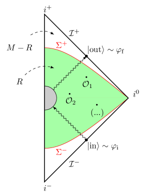
Figure 1: Sub-region $R$ of the full Minkowski spacetime $M$.

One understands from this diagram that the observables are inserted into correlation functions strictly after and before the insertion of the Noether current on $\varSigma^{\pm}$. The sub-region $R$ is such that $\partial R=\varSigma^{+}\cup i^{0}\cup\varSigma^{-}$ and thus $R\cap\partial M=\partial R\cap\partial M=i^{0}$. The reason why one has to consider this sub-region is that the change of field variable leaving invariant the path integral boundary conditions $(\varphi^{i},\varphi^{f})$, which are defined on $(\mathcal{I}^{-}\cup i^{-},\mathcal{I}^{+}\cup i^{+})$, and leading to the Ward identity (2.23) is only valid in $R$.

After having performed this change of field variable, one can push $\varSigma^{\pm}$ arbitrarily close to null infinities $\mathcal{I}^{\pm}$ and analyze the consequences of (2.23) for asymptotic symmetries. Notice that the past (future) boundary of $\varSigma^{+}$ ($\varSigma^{-}$) is $\mathcal{I}^{+}_{-}$ ($\mathcal{I}^{-}_{+}$), which is precisely where the corner charges (2.22) are defined when the Cauchy hypersurface is taken to be $\mathcal{I}^{+}$ ($\mathcal{I}^{-}$).

We can now apply the theorem (2.17) on the BRST Noether current in (2.23) to obtain

$$\left\langle\int_{\mathcal{I}^{+}_{-}}\Big{(}q_{\text{cl},c^{A}_{1}}+q_{\varPsi}\Big{)}\mathcal{O}_{1}\cdots\mathcal{O}_{n}\right\rangle-\left\langle\mathcal{O}_{1}\cdots\mathcal{O}_{n}\int_{\mathcal{I}^{-}_{+}}\Big{(}q_{\text{cl},c^{A}_{1}}+q_{\varPsi}\Big{)}\right\rangle=0.$$ (2.24)

This identity results from the properties of Green functions

$$\langle\big{(}sG_{\varPsi}\big{)}\mathcal{O}_{1}\cdots\mathcal{O}_{n}\rangle=\langle f\big{(}\text{EoM}\big{)}\mathcal{O}_{1}\cdots\mathcal{O}_{n}\rangle=0.$$ (2.25)

So far, the Ward identity (2.24) is empty because it has ghost number one. We can obtain a ghost number zero identity by considering

$$\left.\int_{R}dy\ \lambda^{A}(y)\frac{\delta\eqref{WI_q_gauge}}{\delta c^{A}_{1}(y)}\right|_{c^{A}_{1}=c^{P}_{2}=0}=0,$$ (2.26)

where the (ghost number zero) classical infinitesimal gauge parameter $\lambda^{A}(y)$ is in a formal one to one correspondence with the primary ghost $c^{A}_{1}(y)$. Getting non-trivial ghost number zero consequences from a ghost number one BRST Ward identity is a common practice, as when one proves the gauge independence and the unitarity properties for the physical $\mathcal{S}$-matrix from the bulk BRST master equation of a gauge theory.

Because of (2.2), the only term in $q_{\text{cl},c^{A}_{1}}+q_{\varPsi}$ which survives the operation (2.26) is the classical Noether charge $q_{\text{cl},c^{A}_{1}}$. Moreover, in order not to lose half of the information of (2.24) when applying (2.26), we need to antipodally identify the ghost field components $c^{A}_{1}\big{|}_{\mathcal{I}^{+}_{-}}=c^{A}_{1}\big{|}_{\mathcal{I}^{-}_{+}}$. The standard antipodal matching condition $\lambda^{A}(z,\bar{z})\big{|}_{\mathcal{I}^{+}_{-}}=\lambda^{A}(z,\bar{z})\big{|}_{\mathcal{I}^{-}_{+}}$ [15] of the large gauge symmetry parameters that lead to non-vanishing charges (2.22) naturally follows.

We can finally apply the LSZ reduction formula to (2.26) to obtain

$$\langle\rm out\rvert[Q_{\lambda^{A}},\mathcal{S}]\lvert\rm in\rangle=0,$$ (2.27)

with the notations $\left\langle\mathcal{O}_{1}\cdots\mathcal{O}_{n}\right\rangle\big{|}_{\rm LSZ}=\langle\rm out\rvert\mathcal{S}\lvert\rm in\rangle$ and $[Q_{\lambda^{A}},\mathcal{S}]=Q^{+}_{\lambda^{A}}\mathcal{S}-\mathcal{S}Q^{-}_{\lambda^{A}}$ where $Q^{\pm}_{\lambda^{A}}$ are given by (2.22) integrated over $\mathcal{I}^{+}_{-}$ and $\mathcal{I}^{-}_{+}$, respectively. This provides a universal gauge independent derivation of the invariance of the $\mathcal{S}$-matrix under asymptotic symmetries. The holographic Ward identity (2.27) is a physical consequence of the BRST Noether 1.5th theorem (2.17). The potential loop corrections to this Ward identity have been algebraically classified in [16]. They correspond to loop corrections of the associated soft theorem [59, 60, 61, 62, 63, 64, 65].

A last important remark is that we need to assume that the $\lvert\rm in\rangle$ and $\lvert\rm out\rangle$ states are in the same asymptotic symmetry frame of the degenerate vacuum after taking the LSZ reduction formula. This constitutes another matching condition and it is necessary in order to derive soft theorems from (2.27) by using standard perturbative quantum field theory techniques.

3 Symplectic structure

In this Section, we repeatedly make use of trigraded local forms that are part of the BRST covariant phase space [16]. We recall their definition and basic properties in Appendix B.

A symplectic structure can always be defined from the gauge dependent local symplectic potential $\tilde{\theta}$ of (2.1), which is a one-form on the field space. It is based on the symplectic two-form

$$\varOmega\equiv\int_{\varSigma}\delta\tilde{\theta},$$ (3.1)

which is defined for an arbitrary codimension one hypersurface $\varSigma$ in the spacetime. The contraction of the symplectic two-form (3.1) along the ghost number one field space vector field $V$ (B.4) generating the BRST transformations (2.1) appears in the fundamental canonical relation (3.2), which defines what an integrable charge is. A charge $Q=\int_{\varSigma}dq$ is called integrable or Hamiltonian if

$$I_{V}\varOmega\ \hat{=}\ \delta Q.$$ (3.2)

In this case, if the r.h.s. of (3.2) never vanishes, one says that the symplectic two-form is invertible and it can be inverted by considering

$$I_{V}I_{V}\varOmega\ \hat{=}\ sQ=L_{V}Q\equiv\{Q,Q\},$$ (3.3)

where the definition of $s$ in the BRST covariant phase space (B.5) as the Lie derivative in field space was used. This provides a Poisson bracket for the charges $Q$ such that

$$I_{V}\delta\varPhi^{I}\ \hat{=}\ \{Q,\varPhi^{I}\}.$$ (3.4)

This means that the charges $Q$ canonically generate the symmetry associated with $V$, and this is the reason why they are called integrable or Hamiltonian.

When $V$ is associated with the BRST symmetry (2.1), Eq.(3.2) is actually never satisfied. The reason for this is explained in the next subsection and is based on the fact that the ghosts are actual fields and therefore $\delta c^{A}_{1}$ never vanishes. In this case, we have the following local fundamental canonical relation

$$I_{V}\tilde{\omega}^{\mu}=\delta J^{\mu}_{\rm BRST}-Z^{\mu}+\partial_{\nu}Y^{\mu\nu}$$ (3.5)

for the local symplectic two-form $\tilde{\omega}^{\mu}\equiv\delta\tilde{\theta}^{\mu}$. The obstruction to integrability is measured by the non-integrable part $-Z^{\mu}+\partial_{\nu}Y^{\mu\nu}$ which does not vanish on-shell. Appendix B expresses the quantities $Z^{\mu}$ and $\partial_{\nu}Y^{\mu\nu}$ in terms of those in (2.1) as

$$\partial_{\mu}Z^{\mu} =s(\tilde{E}_{\varPhi^{I}}\delta\varPhi^{I}),$$

$$\partial_{\nu}Y^{\mu\nu} =s\tilde{\theta}^{\mu}+\delta K^{\mu}+Z^{\mu}.$$ (3.6)

The corner quantity $Y^{\mu\nu}$, which is antisymmetric in $(\mu,\nu)$, is referred to as the BRST Noetherian flux.

In the classical ungauge fixed case, without BRST ghost and antighost fields, one can also encounter a fundamental canonical relation with a non-integrable part. Examples are open systems such as asymptotically flat gravity or cases when the symmetry parameter becomes field dependent, as it is often so when studying asymptotic symmetries (see [66, 2] for reviews). In this situation, one can define a modified charge bracket (3.3) such that the action of the symmetry on the phase space is still generated by (3.4) but for this modified bracket [27, 31]. The definition of this bracket crucially relies on the split between the integrable and non-integrable part of the fundamental canonical relation. Another approach is to enlarge the field space with edge modes [67, 68, 69, 70, 71, 72, 73] such that in this enlarged phase space, the charges $Q$ are integrable and the Poisson bracket (3.3) can be used [74, 75, 76].

These two approaches are based on the precise form of the non-integrable part of the fundamental canonical relation on-shell. We would like to extend these constructions, or at least one of them, to our gauge fixed BRST fundamental canonical relation (3.5). This means that we need an expression of the BRST Noetherian flux $Y$ (3) in terms of the gauge dependent charges $q=q_{\text{cl},c^{A}_{1}}+q_{\varPsi}$ of the BRST Noether theorem (2.17).

3.1 BRST Noetherian flux

We start by analyzing the classical part $Y_{\rm cl}$ of $Y$, namely the part that does not depend on the gauge fixing functional $\varPsi$ but simply on the gauge invariant Lagrangian $L$. We use the tools of Appendix B and introduce the BRST anomaly operator to express $Y_{\rm cl}$ in terms of the classical corner Noether charges $q_{\text{cl},c^{A}_{1}}$ that appear in (2.9).

When ghost fields are not introduced, it has been shown in [31] that the most general expression for $Y_{\rm cl}$ is obtained by introducing the so-called anomaly operator [31, 77, 78, 79]. We now extend this construction to the case when ghost fields are present.

Given that the BRST operator (2.1) may describe both an internal gauge symmetry with ghosts $\tilde{c}^{A}$ and a spacetime symmetry with vector ghost $\xi$, we define

$$\mathsf{C}\equiv c^{A}_{1}=\{\tilde{c}^{A},\xi\}.$$ (3.7)

If the theory under study has no spacetime symmetry then $\mathsf{C}$ simply reduces to $\tilde{c}^{A}$. Here we keep $\tilde{c}^{A}$ and $\xi$ to stay as general as possible. In this case, as explained in appendix B, we can define the Lie derivative in spacetime $\mathcal{L}_{\xi}=i_{\xi}d-di_{\xi}$ as in (B.6) and we know that the action of the BRST operator on the fields $\phi^{i}$ will contain such a Lie derivative. It is thus interesting to compare the action of $s$ with that of $\mathcal{L}_{\xi}$ by defining

$$\hat{s}\equiv s-\mathcal{L}_{\xi}.$$ (3.8)

By using the trigraded commutations rules of Table 1, one has

$$\hat{s}^{2}=-\mathcal{L}_{\phi}$$ (3.9)

for $\phi\equiv s\xi-\frac{1}{2}\mathcal{L}_{\xi}\xi$. The physical relevance of this $\phi$ is discussed in Appendix B. The operator (3.8) constitutes the first part of the BRST anomaly operator. More precisely, it is exactly the anomaly operator when acting on field space zero forms.

To completely define the action of the BRST anomaly operator on higher field space forms, we notice that any local form $X$ that has ghost number one with a linear dependence on $c^{A}_{1}$ can now be written as $X_{\mathsf{C}}$. Therefore we can consider

$$X_{\delta\mathsf{C}}\equiv X_{\mathsf{C}}\big{|}_{\mathsf{C}=\delta\mathsf{C}}.$$ (3.10)

For instance, the field space vector field (B.4) that generates the BRST transformations (2.1) only on the classical fields $\phi^{i}$ can be written as $V_{\mathsf{C}}$. This means that we can consider the commuting field space vector field $V_{\delta\mathsf{C}}$ valued in the field space one-forms that generates the transformations

$$I_{V_{\delta\mathsf{C}}}\delta\phi^{i}=f^{i}_{A}\delta c^{A}_{1}+f^{\mu i}_{A}\partial_{\mu}(\delta c^{A}_{1}).$$ (3.11)

We can now define what we will call the BRST anomaly operator

$$\varDelta_{\mathsf{C}}\equiv\hat{s}+I_{V_{\delta\mathsf{C}}}=L_{V_{\mathsf{C}}}-\mathcal{L}_{\xi}+I_{V_{\delta\mathsf{C}}}.$$ (3.12)

By making use of Table 1, one gets the following graded commutation relations

$$\delta\varDelta_{\mathsf{C}} =-\varDelta_{\mathsf{C}}\delta+\varDelta_{\delta\mathsf{C}}, d\varDelta_{\mathsf{C}} =-\varDelta_{\mathsf{C}}d,$$

$$I_{V_{\mathsf{C}}}\varDelta_{\mathsf{C}} =\varDelta_{\mathsf{C}}I_{V_{\mathsf{C}}}+I_{V_{s\mathsf{C}}}, s\varDelta_{\mathsf{C}} =-\varDelta_{\mathsf{C}}s-\mathcal{L}_{s\xi}-L_{V_{\delta\mathsf{C}}}I_{V_{\mathsf{C}}},$$ (3.13)

where $\varDelta_{\delta\mathsf{C}}\equiv L_{V_{\delta\mathsf{C}}}-\mathcal{L}_{\delta\xi}$.

Let us now use the operator (3.12) to express $Y_{\rm cl}$ in terms of $q_{\delta\mathsf{C}}\equiv q_{\text{cl},\delta c^{A}_{1}}$. In the following computations, we have to keep in mind that we can only act with $\varDelta_{\mathsf{C}}$ on classical quantities that do not depend on the ghosts because $I_{V_{\delta\mathsf{C}}}$ is only well defined on classical fields (3.11). We must also pay extra attention to the various signs appearing in the computations due to the trigrading. For instance if we work with spacetime differential forms $\phi^{i}$ rather than spacetime multi-vector fields as in (3.11), we use $I_{V_{\delta\mathsf{C}}}\delta\phi^{i}=-(s\phi^{i})\big{|}_{\mathsf{C}=\delta\mathsf{C}}$.

We start by noticing that the gauge invariant Lagrangian $L$, which is a spacetime top-form, can be anomalous in the sense that

$$sL=dK_{\mathsf{C}}\quad\quad\text{and}\quad\quad\mathcal{L}_{\xi}L=-di_{\xi}L\neq sL\quad\quad\Longrightarrow\quad\quad\hat{s}L\neq 0.$$ (3.14)

This may happen when the BRST symmetry is associated with more than just the diffeomorphism symmetry labeled by $\xi$, or when one imposes specific boundary conditions by adding a boundary Lagrangian to $L$, for example the Gibbons-Hawking boundary term in general relativity. We then define the anomaly of a Lagrangian as

$$\varDelta_{\mathsf{C}}L=\hat{s}L=da_{\mathsf{C}}\qquad\text{with}\qquad a_{\mathsf{C}}=K_{\mathsf{C}}+i_{\xi}L,$$ (3.15)

which leads to the relation

$$\varDelta_{\delta\mathsf{C}}L=-da_{\delta\mathsf{C}}.$$ (3.16)

We need other identities coming from the definition of the equations of motion $E=\delta L-d\theta$. In Appendix B, it is shown that

$$I_{V_{\mathsf{C}}}E =dC_{\mathsf{C}},$$

$$I_{V_{\mathsf{C}}}\theta-a_{\mathsf{C}}+i_{\xi}L =I_{V_{\mathsf{C}}}\theta-K_{\mathsf{C}}=-C_{\mathsf{C}}+dq_{\mathsf{C}},$$ (3.17)

from which we deduce

$$I_{V_{\delta\mathsf{C}}}E =-dC_{\delta\mathsf{C}},$$

$$I_{V_{\delta\mathsf{C}}}\theta =-C_{\delta\mathsf{C}}-dq_{\delta\mathsf{C}}+K_{\delta\mathsf{C}}=-C_{\delta\mathsf{C}}-dq_{\delta\mathsf{C}}+a_{\delta\mathsf{C}}-i_{\delta\xi}L.$$ (3.18)

By using (3) and (3.1), we can now compute the anomaly of the equations of motion. We get

$$\varDelta_{\mathsf{C}}E =sE-\mathcal{L}_{\xi}E+I_{V_{\delta\mathsf{C}}}E=d(Z_{\rm cl}+i_{\xi}E-C_{\delta\mathsf{C}}).$$ (3.19)

The anomaly of the local symplectic potential is obtained by using (3.1), (3.15), (3.16), (3.19) and by computing

$$-d\delta a_{\mathsf{C}} =\delta\varDelta_{\mathsf{C}}L=-\varDelta_{\mathsf{C}}\delta L+\varDelta_{\delta\mathsf{C}}L=-\varDelta_{\mathsf{C}}E+d(\varDelta_{\mathsf{C}}\theta-a_{\delta\mathsf{C}})$$

$$\Longrightarrow\quad\varDelta_{\mathsf{C}}\theta \equiv dA_{\mathsf{C}}-\delta a_{\mathsf{C}}+a_{\delta\mathsf{C}}+Z_{\rm cl}+i_{\xi}E-C_{\delta\mathsf{C}}.$$ (3.20)

This equation defines the symplectic anomaly $A_{\mathsf{C}}$.

We can finally compute the Noetherian flux $dY_{\rm cl}$ defined in (3). We find

$$dY_{\rm cl}= \ s\theta+\delta K_{\mathsf{C}}-Z_{\rm cl}$$

$$= \ \varDelta_{\mathsf{C}}\theta+i_{\xi}d\theta-di_{\xi}\theta-I_{V_{\delta\mathsf{C}}}\theta+\delta K_{\mathsf{C}}-Z_{\rm cl}$$

$$= \ dA_{\mathsf{C}}-\delta a_{\mathsf{C}}+a_{\delta\mathsf{C}}+Z_{\rm cl}+i_{\xi}E-C_{\delta\mathsf{C}}+i_{\xi}\delta L-i_{\xi}E-di_{\xi}\theta+C_{\delta\mathsf{C}}+dq_{\delta\mathsf{C}}-a_{\delta\mathsf{C}}$$

$$+i_{\delta\xi}L+\delta(a_{\mathsf{C}}-i_{\xi}L)-Z_{\rm cl}$$

$$= \ d\big{(}q_{\delta\mathsf{C}}-i_{\xi}\theta+A_{\mathsf{C}}\big{)}.$$ (3.21)

This expression of the Noetherian flux is in agreement with that of [31] modulo flips of signs because of the different statistics due to the ghost number. Notice that we didn’t have to assume that the equations of motion were anomaly free, namely that $\varDelta_{\mathsf{C}}E=0$, to derive this result. Another important thing to notice is that the BRST Noetherian flux does not depend on the anomaly of the Lagrangian but only on the symplectic anomaly. The expression (3.1) also shows that in the BRST case, since $\delta\mathsf{C}$ never vanishes, the local fundamental canonical relation (3.5) always has a non-integrable part.

3.2 Gauge fixed fundamental canonical relation

We now turn to the determination of the gauge dependence of the non-integrable part $-Z^{\mu}+\partial_{\nu}Y^{\mu\nu}$ of the fundamental canonical relation (3.5) on-shell. We come back to spacetime multi-vector fields for the following computations because it is easier for keeping track of the integrations by part.

The computation of $Z^{\mu}$ has already been done in (2.1). Indeed, by using the constraints $G_{\varPhi^{I}}=0$, we obtain

$$Z^{\mu} =-(-1)^{\epsilon(\tilde{E}_{\phi^{i}})}\tilde{E}_{\phi^{i}}\left(\frac{\partial f^{i}_{B}}{\partial\partial_{\mu}\phi^{j}}\delta\phi^{j}c^{B}_{1}+f^{\mu i}_{B}\delta c^{B}_{1}\right)-(-1)^{\epsilon(\tilde{E}_{c^{A}_{1}})}\tilde{E}_{c^{A}_{1}}\left(M^{\mu A}_{P}\delta c^{P}_{2}-M^{\mu A}_{BC}c^{B}_{1}\delta c^{C}_{1}\right)$$

$$\quad+(-1)^{\epsilon(\tilde{E}_{c^{P}_{2}})}\tilde{E}_{c^{P}_{2}}\varGamma^{\mu P}_{BQ}c^{B}_{1}\delta c^{Q}_{2}\quad\Longrightarrow\quad Z^{\mu}\ \hat{=}\ 0.$$ (3.22)

The fact that $Z^{\mu}$ vanishes on-shell was conjectured in [16], it is now proven by (3.2). Notice that this is in agreement with the ungauge fixed case, in which the on-shell vanishing of $C_{\delta\mathsf{C}}$ is implied by Noether’s second theorem.

Getting the gauge dependence $\partial_{\nu}Y^{\mu\nu}_{\rm gauge}$ of $\partial_{\nu}Y^{\mu\nu}$ is a bit more involved. A useful thing to remember when performing this computation is the expression $\partial_{\nu}Y^{\mu\nu}_{\rm cl}$ of the previous subsection in the ungauge fixed case. Guided by this expression, we would like to express $\partial_{\nu}Y^{\mu\nu}_{\rm gauge}$ in terms of $q_{\varPsi}\big{|}_{\mathsf{C}=\delta\mathsf{C}}$ where $q_{\varPsi}$ are the gauge charges defined in (2.2). This guess will be helpful when performing the various integrations by part appearing in the computation of $\partial_{\nu}Y^{\mu\nu}_{\rm gauge}$.

From (2.1) we know that $K^{\mu}_{\rm gauge}=0$ so by using (2.1) and (3.2) we get

$$\partial_{\nu}Y^{\mu\nu}_{\rm gauge} =s\theta^{\mu}_{\rm gauge}+Z^{\mu}_{\rm gauge}$$

$$=(-1)^{\epsilon(F_{\phi^{i}})}\Big{(}sF_{\phi^{i}}+\tilde{E}_{\phi^{i}}-E_{\phi^{i}}\Big{)}\Big{(}\frac{\partial f^{i}_{B}}{\partial\partial_{\mu}\phi^{j}}\delta\phi^{j}c^{B}_{1}+f^{\mu i}_{B}\delta c^{B}_{1}\Big{)}$$

$$\quad-(-1)^{\epsilon(F_{c^{A}_{1}})}\Big{(}sF_{c^{A}_{1}}+\tilde{E}_{c^{A}_{1}}\Big{)}\Big{(}M^{\mu A}_{BC}c^{B}_{1}\delta c^{C}_{1}-M^{\mu A}_{P}\delta c^{P}_{2}\Big{)}$$

$$\quad-(-1)^{\epsilon(F_{c^{P}_{2}})}\Big{(}sF_{c^{P}_{2}}+\tilde{E}_{c^{P}_{2}}\Big{)}\varGamma^{\mu P}_{BQ}c^{B}_{1}\delta c^{Q}_{2}$$

$$\quad+F_{\phi^{i}}s\Big{(}\frac{\partial f^{i}_{B}}{\partial\partial_{\mu}\phi^{j}}\delta\phi^{j}c^{B}_{1}+f^{\mu i}_{B}\delta c^{B}_{1}\Big{)}-F_{c^{A}_{1}}s\Big{(}M^{\mu A}_{BC}c^{B}_{1}\delta c^{C}_{1}-M^{\mu A}_{P}\delta c^{P}_{2}\Big{)}$$

$$\quad-F_{c^{P}_{2}}s\Big{(}\varGamma^{\mu P}_{BQ}c^{B}_{1}\delta c^{Q}_{2}\Big{)}.$$ (3.23)

We will divide the computation of this boundary term in three main steps, each of them corresponding to the dependence of (3.2) in (i) $F_{\phi^{i}}$, (ii) $F_{c^{A}_{1}}$ and (iii) $F_{c^{P}_{2}}$. Given that this computation must be valid off-shell, we use the definition of the equations of motion in (2.1) to reexpress $sF_{\varPhi^{I}}+\tilde{E}_{\varPhi^{I}}$ in (3.2). We must also remember that our parametrization for the BRST transformations (2.1) is such that $\frac{\partial f^{i}_{B}}{\partial\partial_{\mu}\phi^{j}}$ is field independent so $s\Big{(}\frac{\partial f^{i}_{B}}{\partial\partial_{\mu}\phi^{j}}\Big{)}=0$.

(i) The $F_{\phi^{i}}$ dependent terms in (3.2) are:

$$\partial_{\nu}Y^{\mu\nu}_{\rm gauge} \supset\bigg{(}-F_{\phi^{k}}\Big{(}\frac{\partial f^{k}_{A}}{\partial\phi^{i}}c^{A}_{1}+\frac{\partial f^{\nu k}_{A}}{\partial\phi^{i}}\partial_{\nu}c^{A}_{1}\Big{)}+\partial_{\nu}\Big{(}F_{\phi^{k}}\frac{\partial f^{k}_{A}}{\partial\partial_{\nu}\phi^{i}}c^{A}_{1}\Big{)}\bigg{)}\bigg{(}\frac{\partial f^{i}_{B}}{\partial\partial_{\mu}\phi^{j}}\delta\phi^{j}c^{B}_{1}+f^{\mu i}_{B}\delta c^{B}_{1}\bigg{)}$$

$$\quad+\bigg{(}F_{\phi^{i}}f^{i}_{A}-\partial_{\nu}\Big{(}F_{\phi^{i}}f^{\nu i}_{A}\Big{)}\bigg{)}\bigg{(}M^{\mu A}_{BC}c^{B}_{1}\delta c^{C}_{1}-M^{\mu A}_{P}\delta c^{P}_{2}\bigg{)}-F_{\phi^{i}}\frac{\partial f^{i}_{B}}{\partial\partial_{\mu}\phi^{j}}\bigg{(}\delta\Big{(}f^{j}_{A}c^{A}_{1}$$

$$\quad+f^{\nu j}_{A}\partial_{\nu}c^{A}_{1}\Big{)}c^{B}_{1}+\delta\phi^{j}\Big{(}\gamma^{B}_{\ P}c^{P}_{2}+M^{\nu B}_{P}\partial_{\nu}c^{P}_{2}+\gamma^{B}_{\ AC}c^{A}_{1}c^{C}_{1}+M^{\nu B}_{AC}c^{A}_{1}\partial_{\nu}c^{C}_{1}\Big{)}\bigg{)}$$

$$\quad+F_{\phi^{i}}\bigg{(}\frac{\partial f^{\mu i}_{B}}{\partial\phi^{j}}s\phi^{j}\delta c^{B}_{1}-f^{\mu i}_{B}\delta\Big{(}\gamma^{B}_{\ P}c^{P}_{2}+M^{\nu B}_{P}\partial_{\nu}c^{P}_{2}+\gamma^{B}_{\ AC}c^{A}_{1}c^{C}_{1}+M^{\nu B}_{AC}c^{A}_{1}\partial_{\nu}c^{C}_{1}\Big{)}\bigg{)}$$ (3.24)

We can now group these terms by their $1$-form in field space dependence. By using (A.2), (A.3) and one integration by part, the $\delta c^{P}_{2}$ 1-form terms regroup into a boundary term, which is

$$\partial_{\nu}Y^{\mu\nu}_{\rm gauge}\supset\partial_{\nu}\Big{(}F_{\phi^{i}}f^{\nu i}_{A}M^{\mu A}_{P}\delta c^{P}_{2}\Big{)}.$$ (3.25)

As it should, this boundary term is antisymmetric in $(\mu,\nu)$ by (A.2).

The $\delta c^{A}_{1}$ 1-form terms become a boundary term by (A.5), (A.6), (A.7) and two integrations by part, namely

$$\partial_{\nu}Y^{\mu\nu}_{\rm gauge}\supset\partial_{\nu}\bigg{(}F_{\phi^{i}}\Big{(}\frac{\partial f^{i}_{B}}{\partial\partial_{\nu}\phi^{j}}f^{\mu j}_{A}-f^{\nu i}_{C}M^{\mu C}_{BA}\Big{)}c^{B}_{1}\delta c^{A}_{1}\bigg{)}.$$ (3.26)

It is indeed antisymmetric in $(\mu,\nu)$ by (A.6).

For the $\delta\phi^{j}$ 1-form terms, we need additional constraints. They come from imposing $\frac{\partial(s^{2}\phi^{i})}{\partial\partial_{\mu}\phi^{j}}=0$. In fact, since the consequences of $s^{2}\phi^{i}=0$ are obtained by expanding in a polynomial basis of ghost fields and their derivatives, as in (2.1), imposing $\frac{\partial(s^{2}\phi^{i})}{\partial\partial_{\mu}\phi^{j}}=0$ leads us to new constraints that are basically the derivative with respect to $\partial_{\mu}\phi^{j}$ of the constraints (A.1)-(A.7). The fact that the parametrizing functions of (2.1) are polynomial in the fields is crucial here to be able to use identities of the type

$$\frac{\partial(\partial_{\nu}\gamma^{A}_{\ BC})}{\partial\partial_{\mu}\phi^{j}}=\delta^{\mu}_{\nu}\frac{\partial\gamma^{A}_{\ BC}}{\partial\phi^{j}}.$$ (3.27)

We can now use the new constraints coming from (A.1), (A.3), (A.4), (A.5) and one integration by part in (3.2) to show that the $\delta\phi^{j}$ 1-form terms indeed reduce to a boundary term, that is

$$\partial_{\nu}Y^{\mu\nu}_{\rm gauge}\supset\partial_{\nu}\bigg{(}F_{\phi^{i}}\frac{\partial f^{i}_{A}}{\partial\partial_{\nu}\phi^{j}}\frac{\partial f^{j}_{B}}{\partial\partial_{\mu}\phi^{k}}c^{A}_{1}\delta\phi^{k}c^{B}_{1}\bigg{)}=0.$$ (3.28)

This boundary term vanishes by a new constraint that comes from acting with $\frac{\partial}{\partial(\partial_{\nu}\partial_{\mu}\phi^{k})}$ on the constraint (A.4). It is actually not a surprise that this boundary term does not contribute since there is no way to prove its antisymmetry in $(\mu,\nu)$.

(ii) The $F_{c^{A}_{1}}$ dependent terms in (3.2) are:

$$\partial_{\nu}Y^{\mu\nu}_{\rm gauge} \supset-F_{c^{A}_{1}}\frac{\partial}{\partial\phi^{i}}\big{(}sc^{A}_{1}\big{)}\Big{(}\frac{\partial f^{i}_{B}}{\partial\partial_{\mu}\phi^{j}}\delta\phi^{j}c^{B}_{1}+f^{\mu i}_{B}\delta c^{B}_{1}\Big{)}$$

$$\quad-\Big{(}F_{c^{D}_{1}}\big{(}\gamma^{D}_{\ \{AE\}}c^{E}_{1}+M^{\nu D}_{AE}\partial_{\nu}c^{E}_{1}\big{)}+\partial_{\nu}\big{(}F_{c^{D}_{1}}M^{\nu D}_{EA}c^{E}_{1}\big{)}\Big{)}\Big{(}M^{\mu A}_{BC}c^{B}_{1}\delta c^{C}_{1}-M^{\mu A}_{P}\delta c^{P}_{2}\Big{)}$$

$$\quad+\Big{(}F_{c^{D}_{1}}\gamma^{D}_{\ P}-\partial_{\nu}\big{(}F_{c^{D}_{1}}M^{\nu D}_{P}\big{)}\Big{)}\varGamma^{\mu P}_{BQ}c^{B}_{1}\delta c^{Q}_{2}-F_{c^{A}_{1}}s\Big{(}M^{\mu A}_{BC}c^{B}_{1}\delta c^{C}_{1}-M^{\mu A}_{Q}\delta c^{Q}_{2}\Big{)}$$ (3.29)

By using (A.10), (A.11), (A.12) and two integrations by part, the $\delta c^{P}_{2}$ 1-form terms regroup into a boundary term, which is

$$\partial_{\nu}Y^{\mu\nu}_{\rm gauge}\supset\partial_{\nu}\bigg{(}F_{c^{D}_{1}}\Big{(}M^{\nu D}_{EA}M^{\mu A}_{Q}-M^{\nu D}_{P}\varGamma^{\mu P}_{EQ}\Big{)}c^{E}_{1}\delta c^{Q}_{2}\bigg{)}.$$ (3.30)

As it should, this boundary term is antisymmetric in $(\mu,\nu)$ by (A.10).

The $\delta c^{A}_{1}$ 1-form terms become a boundary term by (A.9), (A.12), (A), (A.15), (A.16) and one integration by part, namely

$$\partial_{\nu}Y^{\mu\nu}_{\rm gauge}\supset-\partial_{\nu}\Big{(}F_{c^{D}_{1}}M^{\nu D}_{EA}M^{\mu A}_{BC}c^{E}_{1}c^{B}_{1}\delta c^{C}_{1}\Big{)}.$$ (3.31)

This term either vanishes or is antisymmetric in $(\mu,\nu)$ by (A.15).

For the $\delta\phi^{j}$ 1-form terms, we find that they all vanish by new constraints that come from acting with $\frac{\partial}{\partial(\partial_{\mu}\phi^{j})}$ on the constraints (A.8), (A.11), (A) and (A).

(iii) The $F_{c^{P}_{2}}$ dependent terms in (3.2) are:

$$\partial_{\nu}Y^{\mu\nu}_{\rm gauge} \supset-F_{c^{P}_{2}}\frac{\partial}{\partial\phi^{i}}\big{(}sc^{P}_{2}\big{)}\Big{(}\frac{\partial f^{i}_{B}}{\partial\partial_{\mu}\phi^{j}}\delta\phi^{j}c^{B}_{1}+f^{\mu i}_{B}\delta c^{B}_{1}\Big{)}$$

$$\quad+F_{c^{P}_{2}}\Big{(}\beta^{P}_{\ \{ACD\}}c^{C}_{1}c^{D}_{1}+\varGamma^{P}_{\ QA}c^{Q}_{2}+\varGamma^{\nu P}_{AQ}\partial_{\nu}c^{Q}_{2}\Big{)}\Big{(}M^{\mu A}_{EF}c^{E}_{1}\delta c^{F}_{1}-M^{\mu A}_{R}\delta c^{R}_{2}\Big{)}$$

$$\quad+\Big{(}F_{c^{P}_{2}}\varGamma^{P}_{\ QC}c^{C}_{1}-\partial_{\nu}\big{(}F_{c^{P}_{2}}\varGamma^{\nu P}_{CQ}c^{C}_{1}\big{)}\Big{)}\varGamma^{\mu Q}_{DR}c^{D}_{1}\delta c^{R}_{2}-F_{c^{P}_{2}}s\Big{(}\varGamma^{\mu P}_{CQ}c^{C}_{1}\delta c^{Q}_{2}\Big{)}$$ (3.32)

The $\delta c^{P}_{2}$ dependent terms can be grouped into the boundary term

$$-\partial_{\nu}\Big{(}F_{c^{P}_{2}}\varGamma^{\nu P}_{CQ}\varGamma^{\mu Q}_{DR}c^{C}_{1}c^{D}_{1}\delta c^{R}_{2}\Big{)}\subset\partial_{\nu}Y^{\mu\nu}_{\rm gauge}$$ (3.33)

by doing one integration by part and making use of (A.18), (A.19), (A.21), (A.22) and (A.24). The boundary term (3.33) again either vanishes or is antisymmetric in $(\mu,\nu)$ by (A.21).

The $\delta c^{A}_{1}$ dependent terms can be shown to vanish by using (A.22), (A.23) and (A.26). It also happens to be the case for the $\delta\phi^{j}$ ones by the constraints obtained from acting with $\frac{\partial}{\partial(\partial_{\mu}\phi^{j})}$ on (A.20), (A.24) and (A.25). This concludes the computation of $\partial_{\nu}Y^{\mu\nu}_{\rm gauge}$.

Given the explicit form (2.2) of the gauge charges, which can be written as

$$q^{\mu\nu}_{\varPsi}=q^{\mu\nu}_{\varPsi,c^{A}_{1}}+q^{\mu\nu}_{\varPsi,c^{P}_{2}}$$ (3.34)

where $q_{\varPsi,c^{A}_{1}}$ does not depend on $c^{P}_{2}$ and $q_{\varPsi,c^{P}_{2}}$ is linear in $c^{P}_{2}$, we can use the fact that $\epsilon(F_{\phi^{i}})=\epsilon(F_{c^{A}_{1}})+1=\epsilon(F_{c^{P}_{2}})$ and the results (3.25), (3.26), (3.30), (3.31) and (3.33) to write

$$\partial_{\nu}Y^{\mu\nu}_{\rm gauge} =(-1)^{\epsilon(F_{\phi^{i}})}\partial_{\nu}\Big{(}q^{\mu\nu}_{\varPsi,\delta c^{A}_{1}}-\frac{1}{2}q^{\mu\nu}_{\varPsi,\delta c^{P}_{2}}\Big{)}.$$ (3.35)

This is close from our initial guess but with the very important difference that $i_{\xi}\theta_{\rm gauge}$ does not contribute and that there is no gauge dependent equivalent of the symplectic anomaly.

By combining all the results of this section and of section 2.2, the gauge fixed fundamental canonical relation (3.5) takes the following form

$$I_{V}\tilde{\omega}^{\mu}\ \hat{=} \ \delta sG^{\mu}_{\varPsi}+\partial_{\nu}\Big{(}-\delta q^{\mu\nu}_{\text{cl},c^{A}_{1}}+q^{\mu\nu}_{\text{cl},\delta c^{A}_{1}}-\big{(}i_{\xi}\theta\big{)}^{\mu\nu}+\big{(}A_{c^{A}_{1}}\big{)}^{\mu\nu}\Big{)}$$

$$+\partial_{\nu}\bigg{(}\delta\Big{(}q^{\mu\nu}_{\varPsi,c^{A}_{1}}+q^{\mu\nu}_{\varPsi,c^{P}_{2}}\Big{)}+(-1)^{\epsilon(F_{\phi^{i}})}\Big{(}q^{\mu\nu}_{\varPsi,\delta c^{A}_{1}}-\frac{1}{2}q^{\mu\nu}_{\varPsi,\delta c^{P}_{2}}\Big{)}\bigg{)},$$ (3.36)

This determines the explicit gauge dependence of the non-integrable part of the fundamental canonical relation. It slightly differs from the predictions made in [16], in which the gauge charges $q^{\mu\nu}_{\varPsi}$ were not present. To reach this result, every single constraints coming from the nilpotency of the BRST operator have been used, except for (A.17), as well as all equations of motion (2.1) for $\phi^{j}$, $c^{A}_{1}$ and $c^{P}_{2}$.

3.3 Charge bracket

As explained in section 2.3, the global Noether charges

$$Q_{\mathsf{C}}\equiv Q_{\text{cl},c^{A}_{1}}=\int_{\partial\varSigma}dx^{(d-2)}_{\mu\nu}q^{\mu\nu}_{\text{cl},c^{A}_{1}}$$ (3.37)

are non-vanishing only when the ghosts $c^{A}_{1}$ are valued in the asymptotic symmetry algebra $\mathfrak{asg}$. We refer to these particular ghost components as large ghosts and we call them $\mathsf{C}$. The structure of the asymptotic symmetry algebra $\mathfrak{asg}$ is then completely encoded in the action of the large BRST operator $s\equiv L_{V_{\mathsf{C}}}$ on the large ghosts. To see this, let us draw the parallel with the standard ghost number zero large gauge symmetry parameter $\lambda^{A}$, which might be field dependent and whose ghostification is $\mathsf{C}$. One has

$$s\mathsf{C}\in\mathfrak{asg}\quad\quad \longleftrightarrow\quad\quad\textit{The algebra closes:}\quad[\delta_{\lambda_{1}},\delta_{\lambda_{2}}]=\delta_{\llbracket\lambda_{1},\lambda_{2}\rrbracket}$$

$$s^{2}\mathsf{C}=0\quad\quad \longleftrightarrow\quad\quad\textit{Jacobi identity:}\quad\big{\llbracket}\llbracket\lambda_{1},\lambda_{2}\rrbracket,\lambda_{3}\big{\rrbracket}+\text{cyclic}(1,2,3)=0.$$ (3.38)

Here $\delta_{\lambda^{A}}$ generates the transformation (2.1) on the classical fields $\phi^{i}$ where $c^{A}_{1}$ is replaced by $\lambda^{A}$. Notice that when one uses symmetry parameters rather than ghosts, a modified bracket $\llbracket\cdot,\cdot\rrbracket$ needs to be introduced to account for the possible classical field dependence of $\lambda^{A}$. It is defined as [6, 37]

$$\llbracket\lambda_{1},\lambda_{2}\rrbracket^{A}\equiv\gamma^{A}_{\ BC}(\phi)\lambda_{1}^{B}\lambda_{2}^{C}+M^{\mu A}_{BC}(\phi)\lambda_{1}^{B}\partial_{\mu}\lambda_{2}^{C}+\delta_{\lambda_{1}}\lambda_{2}^{A}-\delta_{\lambda_{2}}\lambda_{1}^{A}.$$ (3.39)

We thus understand that it is easier to work with the large ghosts $\mathsf{C}$ and the large BRST operator $s\equiv L_{V_{\mathsf{C}}}$ to represent the asymptotic symmetry algebra. Such large ghosts and large BRST operator have been constructed for the extended BMS4 symmetry, which is the asymptotic symmetry of asymptotically flat gravity in four dimensions, in [38]. They satisfy the l.h.s. of (3.3) by construction.

To make the equivalence (3.3) more concrete, we now show that it is possible to define an algebra of ghost dependent Noether charges $Q_{\mathsf{C}}$ (3.37) with a charge bracket that represents the r.h.s. of (3.3). This charge bracket has to be constructed out of the symplectic $2$-form $\varOmega$ (3.1), which is the building block of the Poisson bracket (3.3) in the integrable case. When the charges are non-integrable, as it is the case in (3.2), we start with the Barnich–Troessaert bracket $\{Q_{\mathsf{C}},Q_{\mathsf{C}}\}\equiv I_{V_{\mathsf{C}}}I_{V_{\mathsf{C}}}\varOmega$ [27]. By integrating (3.2) over $\varSigma$, we thus get

$$\{Q_{\mathsf{C}},Q_{\mathsf{C}}\}\ \hat{=} -sQ_{\mathsf{C}}+Q_{s\mathsf{C}}-\int_{\partial\varSigma}(i_{\xi}I_{V_{\mathsf{C}}}\theta-I_{V_{\mathsf{C}}}A_{\mathsf{C}})$$

$$+sQ_{\varPsi,c^{A}_{1}}+(-1)^{\epsilon(F_{\phi^{i}})}Q_{\varPsi,sc^{A}_{1}}+sQ_{\varPsi,c^{P}_{2}}-\frac{1}{2}(-1)^{\epsilon(F_{\phi^{i}})}Q_{\varPsi,sc^{P}_{2}},$$ (3.40)

where we have used $I_{V}\delta sG^{\mu}_{\varPsi}=s^{2}G^{\mu}_{\varPsi}=0$ and defined

$$Q_{\varPsi}=Q_{\varPsi,c^{A}_{1}}+Q_{\varPsi,c^{P}_{2}}\equiv\int_{\partial\varSigma}dx^{(d-2)}_{\mu\nu}q^{\mu\nu}_{\varPsi,c^{A}_{1}}+\int_{\partial\varSigma}dx^{(d-2)}_{\mu\nu}q^{\mu\nu}_{\varPsi,c^{P}_{2}}.$$ (3.41)

A first thing to notice with the bracket (3.3) is that it depends on the gauge fixing functional $\varPsi$. We certainly don’t want this since it must provide a representation of the asymptotic symmetry algebra which is gauge independent. This bracket also defines the canonical action of the charges $Q_{\mathsf{C}}$ on solution space as in (3.4). Since this is the action of asymptotic symmetries on solution space, which are non-trivial physical symmetries, it cannot depend on the gauge dependent charges (3.41). To circumvent these problems, we simply impose restrictive boundary conditions on the antighosts $\bar{c}_{I}$ and on the Lagrange multiplier fields $b_{I}$ that are compatible with the BRST transformations (2.1),

$$\bar{c}_{I}\Big{|}_{\partial\varSigma}=0\quad\quad\text{and}\quad\quad b_{I}\Big{|}_{\partial\varSigma}=0.$$ (3.42)

Then by using (2.2), we know that $Q_{\varPsi}$ is a sum of linear terms in $F_{\phi}$, $F_{c^{A}_{1}}$ and $F_{c^{P}_{2}}$. But by definition (2.1), these $F$’s have ghost number $-1$, $-2$ and $-3$, respectively, which means that they must depend on $\bar{c}_{I}$. So by making use of the boundary conditions (3.42), we have

$$Q_{\varPsi}=0.$$ (3.43)

Physically, the boundary conditions (3.42) mean that the gauge has been fixed everywhere except on the corners $\partial\varSigma$. This is the only place where we can do that, because it is precisely here that the gauge symmetry becomes “large” or physical. So all this was possible because the whole gauge dependence of the bracket concentrates on the corners thanks to the BRST Noether theorem (2.17) and the property (3.2).

We are left with the gauge independent bracket

$$\{Q_{\mathsf{C}},Q_{\mathsf{C}}\}=I_{V_{\mathsf{C}}}I_{V_{\mathsf{C}}}\varOmega\ \hat{=}-sQ_{\mathsf{C}}+Q_{s\mathsf{C}}-\int_{\partial\varSigma}(i_{\xi}I_{V_{\mathsf{C}}}\theta-I_{V_{\mathsf{C}}}A_{\mathsf{C}}),$$ (3.44)

which a priori does not represent the r.h.s. of (3.3) yet. What we want is to define a bracket that satisfies

$${\{Q_{\mathsf{C}},Q_{\mathsf{C}}\}}_{L}\ \hat{=}\ Q_{s\mathsf{C}}\quad\quad\Longrightarrow\quad\quad{\big{\{}Q_{\mathsf{C}},{\{Q_{\mathsf{C}},Q_{\mathsf{C}}\}}_{L}\big{\}}}_{L}\ \hat{=}\ Q_{s^{2}\mathsf{C}}=0.$$ (3.45)

The reason for the subscript $L$ is that every single quantity that will appear in the definition of this bracket can be derived from the gauge invariant Lagrangian $L$. A further requirement is that this bracket must be invariant under boundary shifts of the Lagrangian $L\longrightarrow L^{\prime}=L+dl$. Indeed, there is an ambiguity in the split between integrable and non-integrable parts of the fundamental canonical relation (3.2) that comes from the ambiguity in the definition of the local symplectic potential $\delta L^{\prime}=E^{\prime}+d\theta^{\prime}$ with $E^{\prime}=E$ and

$$\theta^{\prime} =\theta-\delta l+d\nu.$$ (3.46)

The bracket (3.45) must be insensitive to this ambiguity, namely one must have

$${\{Q_{\mathsf{C}},Q_{\mathsf{C}}\}}_{L}-Q_{s\mathsf{C}}={\{Q^{\prime}_{\mathsf{C}},Q^{\prime}_{\mathsf{C}}\}}_{L^{\prime}}-Q^{\prime}_{s\mathsf{C}}.$$ (3.47)

By using the various results of section 3.1, we claim that a bracket satisfying (3.45) and (3.47) is given locally by

$${\{q_{\mathsf{C}},q_{\mathsf{C}}\}}_{L} \equiv\frac{1}{2}I_{V_{\mathsf{C}}}I_{V_{\mathsf{C}}}\tilde{\omega}+d\Big{(}\mathcal{L}_{\xi}q_{\mathsf{C}}-I_{V_{\mathsf{C}}}A_{\mathsf{C}}+\kappa-\frac{1}{2}i_{\xi}i_{\xi}L\Big{)},$$ (3.48)

where $\kappa$ is defined as

$$d\kappa\equiv\varDelta_{\mathsf{C}}a_{\mathsf{C}}-i_{\phi}L.$$ (3.49)

The definition of $\kappa$ follows from (3.9), (3.15) and the algebraic Poincaré lemma.

Let us prove that (3.48) has indeed the expected features (3.45)-(3.47) of a bracket and represents the asymptotic symmetry algebra (3.3) without central extension. By using the results of section 3.1 and omitting the $q_{\varPsi}$ dependence of (3.2) which won’t contribute to the global bracket because of (3.43), we compute

$$\frac{1}{2}I_{V_{\mathsf{C}}}I_{V_{\mathsf{C}}}\tilde{\omega}\ \hat{=} \ \frac{1}{2}\Big{(}sdq_{\mathsf{C}}+sI_{V_{\mathsf{C}}}\theta-I_{V_{\mathsf{C}}}Z_{\rm cl}+sK_{\mathsf{C}}\Big{)}$$

$$= \ I_{V_{\mathsf{C}}}s\theta+\frac{1}{2}\Big{(}sC_{\mathsf{C}}-I_{V_{\mathsf{C}}}Z_{\rm cl}\Big{)}$$

$$= \ I_{V_{\mathsf{C}}}\varDelta_{\mathsf{C}}\theta+I_{V_{\mathsf{C}}}\mathcal{L}_{\xi}\theta-I_{V_{\mathsf{C}}}I_{V_{\delta\mathsf{C}}}\theta+\frac{1}{2}\Big{(}sC_{\mathsf{C}}-I_{V_{\mathsf{C}}}Z_{\rm cl}\Big{)}$$

$$= \ I_{V_{\mathsf{C}}}\Big{(}dA_{\mathsf{C}}-\delta a_{\mathsf{C}}+a_{\delta\mathsf{C}}+Z_{\rm cl}+i_{\xi}E+I_{V_{\delta\mathsf{C}}}\theta+dq_{\delta\mathsf{C}}-a_{\delta\mathsf{C}}+i_{\delta\xi}L\Big{)}-I_{V_{\mathsf{C}}}I_{V_{\delta\mathsf{C}}}\theta$$

$$+\mathcal{L}_{\xi}dq_{\mathsf{C}}+\mathcal{L}_{\xi}a_{\mathsf{C}}-\mathcal{L}_{\xi}C_{\mathsf{C}}-\mathcal{L}_{\xi}i_{\xi}L+\frac{1}{2}\Big{(}sC_{\mathsf{C}}-I_{V_{\mathsf{C}}}Z_{\rm cl}\Big{)}$$

$$= \ \frac{1}{2}\Big{(}sC_{\mathsf{C}}+I_{V_{\mathsf{C}}}Z_{\rm cl}\Big{)}-d\Big{(}\mathcal{L}_{\xi}q_{\mathsf{C}}-I_{V_{\mathsf{C}}}A_{\mathsf{C}}+\kappa-\frac{1}{2}i_{\xi}i_{\xi}L-i_{\xi}C_{\mathsf{C}}\Big{)}+dq_{s\mathsf{C}}.$$ (3.50)

To arrive at (3.45), we use (2.9) to write $C^{\mu}_{\mathsf{C}}=E_{\phi^{i}}f^{\mu i}_{A}c^{A}_{1}$ and the classical expression of $Z^{\mu}_{\rm cl}$ given by (3.2) to compute

$$sC^{\mu}_{\mathsf{C}}-I_{V_{\mathsf{C}}}Z^{\mu}_{\rm cl} =(-1)^{\epsilon(E_{\phi^{i}})}\partial_{\nu}\bigg{[}E_{\phi^{i}}\left(c^{B}_{1}c^{A}_{1}\Big{(}\frac{\partial f^{i}_{B}}{\partial\partial_{\nu}\phi^{j}}f^{\mu j}_{A}-M^{\mu C}_{BA}f^{\nu i}_{C}\Big{)}-2c^{P}_{2}M^{\mu B}_{P}f^{\nu i}_{B}\right)\bigg{]}.$$ (3.51)

In this calculation, we used (A.2), (A.3), (A.6), (A.7) and the Noether identity $E_{\phi^{i}}f^{i}_{A}-\partial_{\nu}(E_{\phi^{i}}f^{\nu i}_{C})=0$. The result (3.51) was expected because from the definitions of $C_{\mathsf{C}}$ and $Z$ in appendix B, one has

$$d\big{(}sC_{\mathsf{C}}+I_{V_{\mathsf{C}}}Z\big{)}=0\quad\Longrightarrow\quad sC_{\mathsf{C}}+I_{V_{\mathsf{C}}}Z\equiv dI.$$ (3.52)

Therefore the classical part $I^{\mu\nu}_{\rm cl}$ of $I^{\mu\nu}$ is given by the corner term (3.51). Notice that it has the exact same structure as the $F_{\phi^{i}}$ dependent part of the gauge charges (2.2). We can finally use the definition of the equations of motion (2.1)

$$0\ \hat{=}\ \tilde{E}_{\phi^{i}}=E_{\phi^{i}}+(\text{terms\ proportional\ to }\bar{c}_{I}\text{\ or\ }b_{I})$$ (3.53)

and the boundary conditions (3.42) to obtain

$$\int_{\varSigma}dx^{(d-1)}_{\mu}\Big{(}sC^{\mu}_{\mathsf{C}}-I_{V_{\mathsf{C}}}Z^{\mu}_{\rm cl}\Big{)}=\int_{\partial\varSigma}dx^{(d-2)}_{\mu\nu}I^{\mu\nu}_{\rm cl}\ \hat{=}\ 0.$$ (3.54)

The same reasoning applies to the corner term $di_{\xi}C_{\mathsf{C}}$ of (3.3).

Gathering everything, we find

$$\boxed{{\{Q_{\mathsf{C}},Q_{\mathsf{C}}\}}_{L}\ \hat{=}\ Q_{s\mathsf{C}}}\$$ (3.55)

for the bracket defined by (3.48). One must appreciate that this bracket is constructed out of the gauge dependent local symplectic two-form $\tilde{\omega}$ and leads, for any gauge fixing functional $\varPsi$, to a centerless representation of the asymptotic symmetry algebra (3.55). This is a major result of this paper.

The last property to check is the invariance of (3.55) under boundary shifts $L^{\prime}=L+dl$. The gauge dependent part of $\tilde{\omega}$ is invariant under this shift but the classical quantities transform as

$$E^{\prime} =E, C_{\mathsf{C}}^{\prime} =C_{\mathsf{C}}, Z^{\prime}_{\rm cl} =Z_{\rm cl},$$

$$\theta^{\prime} =\theta-\delta l+d\nu, K^{\prime}_{\mathsf{C}} =K_{\mathsf{C}}-sl, q^{\prime}_{\mathsf{C}} =q_{\mathsf{C}}+I_{V_{\mathsf{C}}}\nu+i_{\xi}l,$$

$$a^{\prime}_{\mathsf{C}} =a_{\mathsf{C}}-\varDelta_{\mathsf{C}}l, A^{\prime}_{\mathsf{C}} =A_{\mathsf{C}}-\varDelta_{\mathsf{C}}\nu, \kappa^{\prime} =\kappa+i_{\phi}l.$$

By using these relations, one can check that

$$\frac{1}{2}I_{V_{\mathsf{C}}}I_{V_{\mathsf{C}}}\tilde{\omega}^{\prime} =\frac{1}{2}I_{V_{\mathsf{C}}}I_{V_{\mathsf{C}}}\tilde{\omega}-dI_{V_{\mathsf{C}}}s\nu, dI_{V_{\mathsf{C}}}A^{\prime}_{\mathsf{C}} =dI_{V_{\mathsf{C}}}A_{\mathsf{C}}-dI_{V_{\mathsf{C}}}\varDelta_{\mathsf{C}}\nu,$$

$$d\mathcal{L}_{\xi}q^{\prime}_{\mathsf{C}} =d\mathcal{L}_{\xi}q_{\mathsf{C}}+dI_{V_{\mathsf{C}}}\mathcal{L}_{\xi}\nu+di_{\xi}di_{\xi}l, dI_{V_{\mathsf{C}}}q^{\prime}_{\delta\mathsf{C}} =dq_{s\mathsf{C}}+dI_{V_{\mathsf{C}}}I_{V_{\delta\mathsf{C}}}\nu+di_{s\xi}l,$$

$$\frac{1}{2}di_{\xi}i_{\xi}L^{\prime} =\frac{1}{2}di_{\xi}i_{\xi}L+\frac{1}{2}di_{\xi}i_{\xi}dl, d\kappa^{\prime} =d\kappa+di_{\phi}l,$$ (3.57)

with $di_{\phi}l=di_{s\xi}l+\frac{1}{2}di_{\xi}i_{\xi}dl-di_{\xi}di_{\xi}l$ by the definition (3.9). For our bracket (3.48), we thus obtain

$${\{q^{\prime}_{\mathsf{C}},q^{\prime}_{\mathsf{C}}\}}_{L^{\prime}}-dq^{\prime}_{s\mathsf{C}}={\{q_{\mathsf{C}},q_{\mathsf{C}}\}}_{L}-dq_{s\mathsf{C}}$$ (3.58)

and therefore (3.47) is satisfied.

3.4 BRST cocycle for asymptotic symmetries

The symplectic BRST framework introduced in this section allows us to systematically define a ghost number two BRST cocycle associated with asymptotic symmetries. To do so, we use (B.15) and (B.17) to write

$$I_{V_{\mathsf{C}}}I_{V_{\mathsf{C}}}\omega=s\Big{(}-C_{\mathsf{C}}+dq_{\mathsf{C}}+I_{V_{\mathsf{C}}}\theta+K_{\mathsf{C}}\Big{)},$$ (3.59)

from which we get

$$sI_{V_{\mathsf{C}}}I_{V_{\mathsf{C}}}\omega=0.$$ (3.60)

Then, by making use of (3.52) and of the classical part of the computation (3.3), the equation (3.60) leads to the off-shell identity

$$0=\frac{1}{2}sI_{V_{\mathsf{C}}}I_{V_{\mathsf{C}}}\omega=sd\Big{(}\mathcal{L}_{\xi}q_{\mathsf{C}}-I_{V_{\mathsf{C}}}A_{\mathsf{C}}+\kappa-\frac{1}{2}i_{\xi}i_{\xi}L-i_{\xi}C_{\mathsf{C}}-I_{\rm cl}-q_{s\mathsf{C}}\Big{)}.$$ (3.61)

This means that if we define the ghost number two and spacetime codimension two quantity

$$\Delta^{2}_{d-2}\equiv\mathcal{L}_{\xi}q_{\mathsf{C}}-I_{V_{\mathsf{C}}}A_{\mathsf{C}}+\kappa-\frac{1}{2}i_{\xi}i_{\xi}L-i_{\xi}C_{\mathsf{C}}-I_{\rm cl}-q_{s\mathsf{C}},$$ (3.62)

then from (3.61) and the algebraic Poincaré lemma, we obtain the descent equations

$$s\Delta^{2}_{d-2} =d\Delta^{3}_{d-3},$$

$$s\Delta^{3}_{d-3} =d\Delta^{4}_{d-4},$$

$$\hskip 6.11723pt\vdots$$

$$s\Delta^{d-1}_{1} =d\Delta^{d}_{0}.$$ (3.63)

It follows that $\Delta^{2}_{d-2}$ is a ghost number two BRST cocycle associated with the large BRST operator $s=L_{V_{\mathsf{C}}}$. This cocycle justifies and extends the model dependent constructions of [37, 38].

Moreover, $\Delta^{2}_{d-2}$ is actually the Barnich–Troessaert bracket ${\{Q_{\mathsf{C}},Q_{\mathsf{C}}\}}_{\rm BT}\equiv\frac{1}{2}I_{V_{\mathsf{C}}}I_{V_{\mathsf{C}}}\varOmega$ [27] because if we use (3.42), (3.48) and (3.62) we find

$${\{Q_{\mathsf{C}},Q_{\mathsf{C}}\}}_{L}\ \hat{=}\ {\{Q_{\mathsf{C}},Q_{\mathsf{C}}\}}_{\rm BT}+Q_{s\mathsf{C}}+\int_{\partial\varSigma}\Delta^{2}_{d-2},$$ (3.64)

so that the important on-shell relation (3.55) leads to

$${\{Q_{\mathsf{C}},Q_{\mathsf{C}}\}}_{\rm BT}\ \hat{=}\ -\int_{\partial\varSigma}\Delta^{2}_{d-2}.$$ (3.65)

The fact that the cocycle (3.62) is the BRST Barnich–Troessaert bracket on-shell justifies the observation of [38, 16] that a top cocycle $\Delta^{1}_{d-1}$, which is responsible for the perturbative corrections of (2.27) and which generates (3.4), could sometimes be the corner charge $Q_{\mathsf{C}}$ itself. Unfortunately, we don’t have a general construction of this $\Delta^{1}_{d-1}$ yet.

We close this section by pointing out the similarities and differences between our charge bracket (3.48) and the one proposed in [31]. In [31], the authors only deal with a spacetime symmetry parametrized by some ghost number zero field dependent vector parameters $\chi$. This means that they have to deal with a particular modified bracket (3.39) defined as

$$\llbracket\chi_{1},\chi_{2}\rrbracket=\mathcal{L}_{\chi_{1}}\chi_{2}+\delta_{\chi_{1}}\chi_{2}-\delta_{\chi_{2}}\chi_{1}.$$ (3.66)

To get a canonical representation of the r.h.s. of (3.3), they define a charge bracket such that ${\{Q_{\chi_{1}},Q_{\chi_{2}}\}}_{L}\ \hat{=}\ Q_{\llbracket\chi_{1},\chi_{2}\rrbracket}$, which therefore automatically satisfies the Jacobi identity. Roughly speaking, in our case, one can think of the bracket (3.66) as being the equivalent of the ghost number two field $\phi$ defined in (3.9) when $\xi$ is the vector ghost associated with $\chi$. However we do not want to define a charge bracket that satisfies ${\{Q_{\xi},Q_{\xi}\}}_{L}\ \hat{=}\ Q_{\phi}$ since it would not satisfy the Jacobi identity. Rather, we want (3.55) to be satisfied, which importantly allows us to treat internal gauge symmetry and spacetime symmetry at the same time. This is a difference of principle between the approach of [31] and that of the present paper.

This explains why our bracket (3.48) has a different structure than that of [31]. Indeed, although the dependence on $\omega$, $\kappa$, and $L$ is the same, our bracket explicitly depends on the symplectic anomaly $A_{\mathsf{C}}$ and the charges via $\mathcal{L}_{\xi}q_{\mathsf{C}}$, whereas the bracket in [31] does not, instead depending on the anomaly $a_{\mathsf{C}}$. This fact also leads to a difference between the expression of our cocycle (3.62) and the one of the 2-cocycle found in [31]. For us, the BRST 2-cocycle (3.62) is the BRST Barnich–Troessaert bracket on-shell whereas in [31], their 2-cocycle $\Delta_{(\chi_{1},\chi_{2})}$ precisely measures the difference between the Barnich–Troessaert bracket and the bracket ${\{Q_{\chi_{1}},Q_{\chi_{2}}\}}_{L}$, that is

$${\{Q_{\chi_{1}},Q_{\chi_{2}}\}}_{L}\ \hat{=}\ {\{Q_{\chi_{1}},Q_{\chi_{2}}\}}_{\rm BT}+\int_{\partial\varSigma}\Delta_{(\chi_{1},\chi_{2})},$$ (3.67)

and can thus be seen as a field dependent central extension.

Establishing a precise relationship between the results of [31] and those of this paper is certainly important and requires more work.

4 Application: Abelian $2$-form coupled to Chern–Simons

To make the notations of the paper more concrete, let us apply Noether’s 1.5th theorem (2.17) to the gauge fixed theory of an abelian $2$-form $B_{2}$ coupled to Chern–Simons in four-dimensions. The Lagrangian is

$$L=\frac{1}{2}G_{3}\star G_{3}$$ (4.1)

with

$$G_{3}=dB_{2}+\operatorname{Tr}\left(AdA+\frac{2}{3}A^{3}\right).$$ (4.2)

This theory is relevant to us for three reasons. First, it has non-trivial asymptotic symmetries associated with the gauge symmetry of the $2$-form, which provide a symmetry interpretation for scalar soft theorems [43, 44]. Second, its study requires introducing ghosts of ghosts to the field space so it justifies the inclusion of $c^{P}_{2}$ in our general derivation and allow us to understand its impact in practice. Third, this curvature $G_{3}$ plays a fundamental role in the Green–Schwartz anomaly compensation mechanism [80, 81].

The field space is thus composed of an abelian $2$-form $B_{\mu\nu}$, its associated ghost $\psi_{\mu}$ with a ghost for this ghost $\phi$, a non-abelian 1-form $A^{a}_{\mu}$ and its associated ghosts $c^{a}$ valued in a Lie algebra $\mathfrak{g}$. The nilpotent BRST transformations (2.1) leaving invariant the Lagrangian (4.1) are given by

$$sA^{a}_{\mu} =\partial_{\mu}c^{a}+f^{a}_{\ bc}A^{b}_{\mu}c^{c},$$

$$sc^{a} =-\frac{1}{2}f^{a}_{\ bc}c^{b}c^{c},$$

$$sB_{\mu\nu} =\partial_{\{\mu}\psi_{\nu\}}+c^{a}\partial_{\{\mu}A^{a}_{\nu\}},$$

$$s\psi_{\mu} =\partial_{\mu}\phi-\frac{1}{2}A^{a}_{\mu}[c,c]^{a},$$

$$s\phi =\frac{1}{6}c^{a}[c,c]^{a},$$ (4.3)

where $[c,c]^{a}=f^{a}_{\ bc}c^{b}c^{c}$ with the structure constants $f_{abc}$ of $\mathfrak{g}$. These transformations naturally derive from the horizontality conditions on $F=dA+A^{2}$ and $G_{3}$ [82], namely

$$\hat{F} \equiv(d+s)(A+c)+(A+c)^{2}=F,$$

$$\hat{G_{3}} \equiv(d+s)(B_{2}+\psi^{1}_{1}+\phi^{2}_{0})+\operatorname{Tr}\left((A+c)\hat{F}-\frac{1}{3}(A+c)^{3}\right)=G_{3}.$$ (4.4)

The nilpotency is ensured by the Bianchi identities

$$\hat{D}\hat{F}=0\quad\quad\text{and}\quad\quad\hat{d}\hat{G}_{3}=\hat{F}\hat{F}=FF.$$ (4.5)

In particular, notice that the invariance of (4.1) under (4) is obvious because the ghost number one component of $\hat{d}G_{3}=FF$ leads to $sG_{3}=0$.

We can now determine the functions parametrizing (2.1) for the specific case of (4). Since the fields entering (4) have certain indices in common and sometimes have more than one index, the abstract indices $i$, $A$ and $P$ in (2.1) will be replaced by the field itself. For instance, if we compare

$$sA^{a}_{\mu} =\partial_{\mu}c^{a}+f^{a}_{\ bc}A^{b}_{\mu}c^{c}\quad\quad\text{with}\quad\quad s\phi^{i}=f^{i}_{A}c^{A}_{1}+f^{\mu i}_{A}\partial_{\mu}c^{A}_{1},$$ (4.6)

we write $\phi^{A^{a}_{\mu}}=A^{a}_{\mu}$, $c^{c^{a}}_{1}=c^{a}$, $c^{\psi_{\rho}}_{1}=\psi_{\rho}$ and thus we deduce

$$f^{A^{a}_{\mu}}_{c^{c}} =f^{a}_{\ bc}A^{b}_{\mu}, f^{\nu A^{a}_{\mu}}_{c^{b}} =\delta^{\nu}_{\mu}\delta^{a}_{b},$$

$$f^{A^{a}_{\mu}}_{\psi_{\rho}} =0, f^{\nu A^{a}_{\mu}}_{\psi_{\rho}} =0.$$ (4.7)

We can do that for each transformations in (4). If we write only the non-vanishing functions, we have

$$f^{B_{\mu\nu}}_{c^{a}} =\partial_{\{\mu}A^{a}_{\nu\}}, f^{\rho B_{\mu\nu}}_{\psi_{\gamma}} =\delta^{\{\rho}_{\mu}\delta^{\gamma\}}_{\nu},$$

$$\gamma^{c^{a}}_{\ c^{b}c^{c}} =-\frac{1}{2}f^{a}_{\ bc}, \beta^{\phi}_{\ c^{a}c^{b}c^{c}} =\frac{1}{6}f^{a}_{\ bc},$$

$$M^{\nu\psi_{\mu}}_{\phi} =\delta^{\nu}_{\mu}, \gamma^{\psi_{\mu}}_{\ c^{b}c^{c}} =-\frac{1}{2}f^{a}_{\ bc}A^{a}_{\mu}.$$ (4.8)

The next step is gauge fixing. We must fix the gauge invariances associated with $c^{a}$, $\psi_{\mu}$ and $\phi$. A judicious choice of gauge for perturbation theory is for instance

$$\partial_{\mu}A^{\mu}_{a}+\frac{1}{2}b_{a}=0,\quad\quad\partial^{\nu}B_{\mu\nu}+\partial_{\mu}L+\frac{1}{2}b_{\mu}=0,\quad\quad\partial^{\mu}\psi_{\mu}=0,$$ (4.9)

where we have introduced trivial BRST doublets $(\bar{c}_{a}^{-1},b_{a}^{0})$, $(\bar{\psi}_{\mu}^{-1},b_{\mu}^{0})$, $(\bar{\phi}^{-2},\bar{\eta}^{-1})$ and $(L^{0},\eta^{1})$. The upper index is the ghost number. These doublets are captured by the last two lines of the parametrization (2.1). They allow us to impose the gauge condition (4.9) by considering

$$L_{\rm GF}=\frac{1}{2}G_{3}\star G_{3}+s\left(\bar{c}^{a}\Big{(}\partial_{\mu}A^{\mu}_{a}+\frac{1}{2}b_{a}\Big{)}+\bar{\psi}^{\mu}\Big{(}\partial^{\nu}B_{\mu\nu}+\partial_{\mu}L+\frac{1}{2}b_{\mu}\Big{)}+\bar{\phi}\partial^{\mu}\psi_{\mu}\right).$$ (4.10)

The only things we need in order to apply the BRST Noether theorem (2.17) to this gauge fixed Lagrangian are the expressions of $F_{\varPhi^{I}}$ and $\Xi^{\mu}$ as defined in (2.1) and the expression of the classical Noether charge $q^{\mu\nu}_{\text{cl},c^{A}_{1}}$. The classical charge is found by applying Noether’s second theorem (2.9) to the ungauge fixed Lagrangian (4.1). In terms of spacetime differential forms, it is given by

$$q_{\text{cl},c^{A}_{1}}=\Big{(}\psi^{1}_{1}+\operatorname{Tr}(cA)\Big{)}\star G_{3}.$$ (4.11)

Then, by acting on the gauge fixing functional of (4.10) with $\delta$, we find

$$F_{A^{a}_{\mu}} =\partial^{\mu}\bar{c}_{a},\quad\quad F_{B_{\mu\nu}}=\partial^{\nu}\bar{\psi}^{\mu},\quad\quad F_{\psi_{\mu}}=-\partial^{\mu}\bar{\phi},\quad\quad F_{L}=\partial_{\mu}\bar{\psi}^{\mu},$$

$$\Xi^{\mu} =-\bar{c}^{a}\delta A^{\mu}_{a}-\bar{\psi}^{\mu}\delta L-\bar{\psi}^{\nu}\delta B_{\rho\nu}\eta^{\rho\mu}+\bar{\phi}\delta\psi^{\mu}.$$ (4.12)

The expressions of $F_{\bar{c}_{I}}$ and $F_{b_{I}}$ are useless for our purpose because these quantities don’t appear in the BRST Noether current (2.17). Notice however than $F_{L}$ does contribute because $L$ is a “$\bar{c}_{I}$” with ghost number zero, which means that the BRST transformation $sL$ enters the parametrization (2.1) through $s\phi^{i}$. We thus have $f^{L}_{\eta}=1$.

Finally, by plugging (4), (4) and (4) into our general result (2.2), we get

$$J^{\mu}_{\rm BRST} =\partial_{\nu}\Big{(}\big{(}\psi^{1}_{1}+\operatorname{Tr}(cA)\big{)}\star G_{3}\Big{)}^{\mu\nu}-2\partial_{\nu}\Big{(}\phi\partial^{\{\nu}\bar{\psi}^{\mu\}}\Big{)}$$

$$\quad+s\Big{(}\bar{c}^{a}sA^{\mu}_{a}+\bar{\psi}^{\mu}\eta+\bar{\psi}^{\nu}(sB_{\rho\nu})\eta^{\rho\mu}-\bar{\phi}s\psi^{\mu}+c^{a}\partial^{\mu}\bar{c}_{a}+\psi_{\nu}\partial^{\{\mu}\bar{\psi}^{\nu\}}+2\phi\partial^{\mu}\bar{\phi}\Big{)}.$$ (4.13)

In the free theory (4.1) without the coupling to Chern–Simons, the Ward identity (2.27) $[Q,\mathcal{S}]=0$ for the classical Noether charge $Q=\int\psi^{1}_{1}\star G_{3}$ would lead us to the scalar soft theorem for the scalar field $\varphi$ dual to the abelian $2$-form through $\star d\varphi=dB_{2}$ [43, 44]. Here we have shown that a specific gauge fixing of this theory can lead to non-trivial gauge dependent Noether charges $Q_{\phi}=\int\phi\star(d\bar{\psi})$. So without the general BRST construction of the Ward identity $[Q,\mathcal{S}]=0$ exposed in section 2.3 that ensures its gauge independence, one could have naively thought that the charge $Q_{\phi}$ for the ghost of ghost must also commute with the $\mathcal{S}$-matrix, therefore making the physical consequences of asymptotic symmetries gauge dependent. This example thus confirms the need for a BRST construction of the holographic Ward identity (2.27). Notice that such gauge dependent charges also appear for asymptotically flat gravity in the de Donder gauge. Their explicit expression was given at the end of section 2.2.

5 Towards a generalization for rank-$2$ BV systems

So far we have only focused on rank-$1$ BV theories. The symmetries of such theories are captured by a BRST operator which is nilpotent off-shell and maps the fields on local field functionals with no mixing with the antifields. This fact is reflected by a linear dependence on the antifields in the BV action.

However not all theories are of this type, as for instance some supergravity theories without auxiliary fields whose infinitesimal gauge transformations only close on-shell. They appear as not being under the control of a genuinely field dependent BRST operator which is nilpotent off-shell and they have a quadratic dependence on the antifields in the BV action. We thus say that such BV theories are of rank 2. It is believed that all supergravities are at most BV systems of rank 2.

Since these theories of interest have gauge symmetries, there are no reasons they don’t exhibit asymptotic symmetries [83]. We should thus be able to study their physical effects through the holographic Ward identities (2.27). Given that this Ward identity is derived from Noether’s 1.5th theorem (2.17), we may question the validity of this theorem for rank-$2$ BV theories. Here we will only test the validity of the 1.5 Noether theorem for the most simple rank-$2$ BV system, that is Yang-Mills theory in the Feynman-’t Hooft gauge without the $b$ field.

We work in an $n$-dimensional Minkowski spacetime $M$ and start with the usual rank-$1$ BV action of Yang–Mills theory, that is

$$L_{\rm BV}=-\frac{1}{4}F_{\mu\nu}F^{\mu\nu}-s\varPhi^{I}{}^{*}\varPhi_{I},$$ (5.1)

where we have introduced antifields ${}^{*}\varPhi_{I}$ for each fields $\varPhi^{I}=\{A^{a}_{\mu},c^{a},\bar{c}_{a},b_{a}\}$. If $p$ is the spacetime form degree and $g$ the ghost number, the grading of an antifield ${}^{*}\varPhi$ is given by

$${}^{*}(\varPhi^{g}_{p})=({}^{*}\varPhi)^{-g-1}_{n-p}.$$ (5.2)

The antifields can be interpreted as sources for the nilpotent BRST transformations of the fields

$$sA^{a}_{\mu} =D_{\mu}c^{a}=\partial_{\mu}c^{a}+[A_{\mu},c]^{a}, s\bar{c}_{a} =b_{a},$$

$$sc^{a} =-\frac{1}{2}[c,c]^{a}, sb_{a} =0,$$ (5.3)

while their nilpotent BRST transformations are defined as

$$s{}^{*}\varPhi_{I}=\frac{\delta^{L}L_{\rm BV}}{\delta\varPhi^{I}}.$$ (5.4)

To reach the Feynman-’t Hooft gauge, we perform the following anticanonical transformation

$$\left\{\begin{aligned} \varPhi^{I}&=\tilde{\varPhi}^{I}\\ {}^{*}\varPhi_{I}&={}^{*}\tilde{\varPhi}_{I}+\frac{\delta^{L}\varPsi}{\delta\varPhi^{I}}\end{aligned}\right.$$

for the gauge fixing functional $\varPsi=\bar{c}_{a}\big{(}\partial^{\mu}A^{a}_{\mu}+\frac{1}{2}b^{a}\big{)}$. Under this transformation, the BV action (5.1) becomes

$$L_{\rm BV}=-\frac{1}{4}F_{\mu\nu}F^{\mu\nu}-s\varPhi^{I}{}^{*}\tilde{\varPhi}_{I}-s\varPsi.$$ (5.5)

The ${}^{*}\tilde{\varPhi}_{I}$’s can now be seen as background fields. Setting them to zero fixes the gauge as in (2.1). What will be useful is that (5.5) with the background fields still satisfies the classical master equation

$$s_{\varPsi}S_{\rm BV}=2\left(\frac{\delta^{L}S_{\rm BV}}{\delta\varPhi^{I}}\frac{\delta^{R}S_{\rm BV}}{\delta{}^{*}\tilde{\varPhi}_{I}}\right)=\int_{M}dK_{\rm BV}$$ (5.6)

for the shifted nilpotent BRST operator

$$s_{\varPsi}\varPhi^{I} =s\varPhi^{I},$$

$$s_{\varPsi}{}^{*}\tilde{\varPhi}_{I} =\frac{\delta^{L}(L_{\rm cl}-s\varPhi^{I}{}^{*}\tilde{\varPhi}_{I}-s\varPsi)}{\delta\varPhi^{I}}.$$ (5.7)

The original motivation was to calculate the Noether current of a Lagrangian with a quadratic dependence in the antifields. To get there, we integrate out the $b^{a}$ field in (5.5) and obtain

$$L_{\rm BV}=-\frac{1}{4}F_{\mu\nu}F^{\mu\nu}-D_{\mu}c^{a}({}^{*}\tilde{A})^{\mu}_{a}+\frac{1}{2}[c,c]^{a}({}^{*}\tilde{c})_{a}+\bar{c}_{a}\partial_{\mu}D^{\mu}c^{a}-\frac{1}{2}\Big{(}\partial^{\mu}A_{\mu}^{a}+({}^{*}\tilde{\bar{c}})^{a}\Big{)}^{2}.$$ (5.8)

This Lagrangian is indeed quadratic in $({}^{*}\tilde{\bar{c}})^{a}$. Its BRST symmetry is governed by the shifted operator (5), which takes the form

$$sA^{a}_{\mu} =D_{\mu}c^{a}, s{}^{*}\tilde{A}^{\mu}_{a} =D_{\nu}F^{\nu\mu}_{a}+[\partial^{\mu}\bar{c},c]_{a}-[{}^{*}\tilde{A}^{\mu},c]_{a}+\partial^{\mu}\partial_{\nu}A^{\nu}_{a}+\partial^{\mu}{}^{*}\tilde{\bar{c}}_{a},$$

$$sc^{a} =-\frac{1}{2}[c,c]^{a}, s{}^{*}\tilde{c}_{a} =D^{\mu}\partial_{\mu}\bar{c}_{a}+[{}^{*}\tilde{c},c]_{a}-D_{\mu}{}^{*}\tilde{A}^{\mu}_{a},$$

$$s\bar{c}^{a} =\partial^{\mu}A_{\mu}^{a}+{}^{*}\tilde{\bar{c}}^{a}, s{}^{*}\tilde{\bar{c}}^{a} =-\partial_{\mu}D^{\mu}c^{a}.$$ (5.9)

The fact that we are dealing with a rank-$2$ BV system now becomes obvious because if one fixes the gauge by setting the background fields to zero, one gets $s^{2}\bar{c}^{a}=\partial^{\mu}D_{\mu}c^{a}\neq 0$ off-shell. The nilpotency is restored on-shell by the equation of motion of $\bar{c}_{a}$.

Since the quantum field theory must explicitly depend on the background fields for the master equation (5.6) to be valid, we must compute the Noether current associated with the BRST symmetry (5) of the rank-$2$ BV Lagrangian (5.8). We have

$$\delta L_{\rm BV} =\tilde{E}_{\varPhi^{I}}\delta\varPhi^{I}+(-1)^{\epsilon(\varPhi^{I})}s\varPhi^{I}\delta({}^{*}\tilde{\varPhi}_{I})+\partial_{\mu}\tilde{\theta}^{\mu}_{\rm BV},$$

$$sL_{\rm BV} =\partial_{\mu}K^{\mu}_{\rm BV}.$$ (5.10)

This provides

$$\tilde{\theta}^{\mu}_{\rm BV} =-\delta A_{\nu}^{a}F^{\mu\nu}_{a}-\delta A^{\mu}_{a}\big{(}[\bar{c},c]^{a}+{}^{*}\tilde{\bar{c}}^{a}+\partial^{\nu}A_{\nu}^{a}\big{)}-\delta c^{a}{}^{*}\tilde{A}^{\mu}_{a}-\bar{c}_{a}D^{\mu}(\delta c^{a})+\partial^{\mu}\bar{c}_{a}\delta c^{a},$$

$$K^{\mu}_{\rm BV} =c^{a}D_{\nu}F^{\nu\mu}_{a}+\frac{1}{2}[c,c]^{a}\big{(}\partial^{\mu}\bar{c}_{a}-{}^{*}\tilde{A}^{\mu}_{a}\big{)}+D^{\mu}c^{a}\big{(}\partial_{\nu}A^{\nu}_{a}+{}^{*}\tilde{\bar{c}}_{a}\big{)}.$$ (5.11)

We can now compute the Noether current by defining the field space vector field $V$ generating the transformations (5) and considering

$$J^{\mu}_{\rm BV}=I_{V}\tilde{\theta}^{\mu}_{\rm BV}-K^{\mu}_{\rm BV}=-C^{\mu}_{\rm BV}+\partial_{\nu}q^{\mu\nu}_{\rm BV},$$ (5.12)

where $\partial_{\mu}C^{\mu}_{\rm BV}=I_{V}\Big{(}\tilde{E}_{\varPhi^{I}}\delta\varPhi^{I}+(-1)^{\epsilon(\varPhi^{I})}s\varPhi^{I}\delta({}^{*}\tilde{\varPhi}_{I})\Big{)}$ and $q^{\mu\nu}_{\rm BV}$ has yet to be determined. We find

$$C^{\mu}_{\rm BV}=2K^{\mu}_{\rm BV}\ \hat{=}\ 2s\Big{(}c^{a}(\partial^{\mu}\bar{c}_{a}-{}^{*}\tilde{A}^{\mu}_{a})+\bar{c}_{a}D^{\mu}c^{a}\Big{)},$$ (5.13)

where we have used the field equations of motion that are given by the BRST transformations of the antifields in (5). Then by using (5) and plugging the off-shell expression of $C^{\mu}$ in (5.12), we get

$$q^{\mu\nu}_{\rm BV}=-c^{a}F^{\mu\nu}_{a}.$$ (5.14)

The BRST Noether 1.5th theorem (2.17) is thus valid for this simple rank-$2$ BV system.

Whether or not this simple example really tells us something non-trivial about rank-$2$ BV systems is unclear. In fact, the structure of the $s$-exact term (5.13) resembles that of the rank-$1$ theory, which consist in keeping the $b^{a}$ field and imposing the Feynman-’t Hooft gauge in the usual way (2.1). By doing so, one obtains [16]

$$C^{\mu}\ \hat{=}\ s(c^{a}\partial^{\mu}\bar{c}_{a}+b^{a}A^{\mu}_{a}).$$ (5.15)

It has indeed the same structure as (5.13) if one sets the antifields to zero and reintroduce the $b^{a}$ field because in this case $s(\bar{c}_{a}D^{\mu}c^{a})=b_{a}D^{\mu}c^{a}=s(b^{a}A^{\mu}_{a})$.

Proving the BRST Noether 1.5th theorem for every rank-$2$ BV theories will be the subject of a future publication.

Acknowledgments

It is a pleasure to thank Glenn Barnich, Marc Bellon and Luca Ciambelli for insightful discussions.

Appendix A Constraints on the BRST transformations

By making use of (2.1), (2.1) and (2.1), the parametrizing functions of the BRST transformations (2.1) must satisfy the following constraints:

$$\bullet\ f^{i}_{A}\gamma^{A}_{P}+f^{\mu i}_{A}\partial_{\mu}\gamma^{A}_{P}=0$$ (A.1)

$$\bullet\ f^{\mu i}_{A}M^{\nu A}_{P}\ \text{is antisymmetric in}\ (\mu,\nu)$$ (A.2)

$$\bullet\ f^{i}_{A}M^{\mu A}_{P}+f^{\mu i}_{A}\gamma^{A}_{P}+f^{\nu i}_{A}\partial_{\nu}M^{\mu A}_{P}=0$$ (A.3)

$$\bullet\ \frac{\partial f^{i}_{A}}{\partial\phi^{j}}f^{j}_{B}+\frac{\partial f^{i}_{A}}{\partial\partial_{\mu}\phi^{j}}\partial_{\mu}f^{j}_{B}+f^{i}_{C}\gamma^{C}_{\ BA}+f^{\mu i}_{C}\partial_{\mu}\gamma^{C}_{\ BA}\ \text{is symmetric in}\ (A,B)$$ (A.4)

$$\bullet\ \frac{\partial f^{i}_{A}}{\partial\phi^{j}}f^{\mu j}_{B}+\frac{\partial f^{i}_{A}}{\partial\partial_{\mu}\phi^{j}}f^{j}_{B}+\frac{\partial f^{i}_{A}}{\partial\partial_{\nu}\phi^{j}}\partial_{\nu}f^{\mu j}_{B}-f^{i}_{C}M^{\mu C}_{AB}-\frac{\partial f^{\mu i}_{B}}{\partial\phi^{j}}f^{j}_{A}+2f^{\mu i}_{C}\gamma^{C}_{\ BA}-f^{\nu i}_{C}\partial_{\nu}M^{\mu C}_{AB}=0$$ (A.5)

$$\bullet\ \frac{\partial f^{i}_{A}}{\partial\partial_{\mu}\phi^{j}}f^{\nu j}_{B}-f^{\mu i}_{C}M^{\nu C}_{AB}\ \text{is antisymmetric in}\ (\mu,\nu)$$ (A.6)

$$\bullet\ \frac{\partial f^{\mu i}_{A}}{\partial\phi^{j}}f^{\nu j}_{B}+f^{\nu i}_{C}M^{\mu C}_{BA}\ \text{is symmetric in}\ \big{(}(\mu,A),(\nu,B)\big{)}$$ (A.7)

$$\bullet\ \frac{\partial\gamma^{A}_{\ P}}{\partial\phi^{j}}f^{j}_{D}+\gamma^{A}_{\ Q}\varGamma^{Q}_{\ PD}+M^{\mu A}_{Q}\partial_{\mu}\varGamma^{Q}_{\ PD}+\gamma^{A}_{\ \{CD\}}\gamma^{C}_{\ P}-M^{\mu A}_{DC}\partial_{\mu}\gamma^{C}_{\ P}=0$$ (A.8)

$$\bullet\ \frac{\gamma^{A}_{\ P}}{\partial\phi^{j}}f^{\mu j}_{D}+M^{\mu A}_{Q}\varGamma^{Q}_{\ PD}+M^{\mu A}_{CD}\gamma^{C}_{\ P}=0$$ (A.9)

$$\bullet\ M^{\mu A}_{Q}\varGamma^{\nu Q}_{DP}-M^{\mu A}_{DQ}M^{\nu Q}_{P}\ \text{is antisymmetric in}\ (\mu,\nu)$$ (A.10)

$$\bullet\ \frac{\partial M^{\mu A}_{P}}{\partial\phi^{j}}f^{j}_{D}+\gamma^{A}_{\ Q}\varGamma^{\mu Q}_{DP}+M^{\nu A}_{Q}\partial_{\nu}\varGamma^{\mu Q}_{DP}+M^{\mu A}_{Q}\varGamma^{Q}_{PD}+\gamma^{A}_{\ \{CD\}}M^{\mu C}_{P}-M^{\mu A}_{DC}\gamma^{C}_{\ P}$$

$$\quad-M^{\nu A}_{DC}\partial_{\nu}M^{\mu C}_{P}=0$$ (A.11)

$$\bullet\ \frac{\partial M^{\mu A}_{P}}{\partial\phi^{j}}f^{\nu j}_{D}+M^{\nu A}_{Q}\varGamma^{\mu Q}_{DP}+M^{\nu A}_{CD}M^{\mu C}_{P}=0$$ (A.12)

$$\bullet\ \gamma^{A}_{\ P}\beta^{P}_{\ DBC}+M^{\mu A}_{P}\partial_{\mu}\beta^{P}_{\ DBC}+\frac{\partial\gamma^{A}_{\ BC}}{\partial\phi^{j}}f^{j}_{D}+\gamma^{A}_{\ \{EC\}}\gamma^{E}_{\ DB}+M^{\mu A}_{BE}\partial_{\mu}\gamma^{E}_{\ DC}$$

$$\quad\ \text{is totally symmetric in}\ (D,B,C)$$ (A.13)

$$\bullet\ \frac{\partial\gamma^{A}_{\ BC}}{\partial\phi^{j}}f^{\mu j}_{D}+\frac{\partial M^{\mu A}_{CD}}{\partial\phi^{j}}f^{i}_{B}-\gamma^{A}_{\ \{EC\}}M^{\mu E}_{BD}+\gamma^{E}_{\ \{DC\}}M^{\mu A}_{BE}+\gamma^{E}_{\ BC}M^{\mu A}_{ED}-M^{\nu A}_{BE}\partial_{\nu}M^{\mu E}_{CD}$$

$$\quad+M^{\mu A}_{E}\beta^{E}_{\ \{DBC\}}\ \text{is symmetric in}\ (B,C)$$ (A.14)

$$\bullet\ M^{\mu A}_{BE}M^{\nu E}_{CD}\ \text{is symmetric in}\ (B,C)\ \text{and/or antisymmetric in}\ (\mu,\nu)$$ (A.15)

$$\bullet\ M^{\mu A}_{EC}M^{\nu E}_{DB}-M^{\nu A}_{DE}M^{\mu E}_{BC}-\frac{\partial M^{\mu A}_{DC}}{\partial\phi^{j}}f^{\nu j}_{B}\ \text{is symmetric in}\ \big{(}(\mu,C),(\nu,B)\big{)}$$ (A.16)

$$\bullet\ \varGamma^{P}_{\ QB}\gamma^{B}_{\ R}\ \text{is antisymmetric in}\ (Q,R)$$ (A.17)

$$\bullet\ \varGamma^{P}_{\ QB}M^{\nu B}_{R}+\varGamma^{\nu P}_{BR}\gamma^{B}_{\ Q}=0$$ (A.18)

$$\bullet\ \varGamma^{\mu P}_{BQ}M^{\nu B}_{R}\ \text{is antisymmetric in}\ \big{(}(\mu,Q),(\nu,R)\big{)}$$ (A.19)

$$\bullet\ -\frac{\partial\varGamma^{P}_{\ QC}}{\partial\phi^{j}}f^{j}_{E}-\varGamma^{P}_{\ RC}\varGamma^{R}_{\ QE}-\varGamma^{\mu P}_{CR}\partial_{\mu}\varGamma^{R}_{\ QE}+\beta^{P}_{\ \{DCE\}}\gamma^{D}_{\ Q}+\varGamma^{P}_{\ QD}\gamma^{D}_{\ CE}\ \text{is symmetric}$$

$$\quad\ \text{in}\ (C,E)$$ (A.20)

$$\bullet\ \varGamma^{\mu P}_{CQ}\varGamma^{\nu Q}_{DR}\ \text{is symmetric in}\ (C,D)\ \text{and/or antisymmetric in}\ (\mu,\nu)$$ (A.21)

$$\bullet\ -\frac{\partial\varGamma^{\mu P}_{BQ}}{\partial\phi^{j}}f^{\nu j}_{E}-\varGamma^{\nu P}_{BR}\varGamma^{\mu R}_{EQ}+\varGamma^{\mu P}_{DQ}M^{\nu D}_{BE}=0$$ (A.22)

$$\bullet\ -\frac{\partial\varGamma^{P}_{\ QC}}{\partial\phi^{j}}f^{\nu j}_{E}-\varGamma^{\nu P}_{CR}\varGamma^{R}_{\ QE}+\varGamma^{P}_{\ QD}M^{\nu D}_{CE}=0$$ (A.23)

$$\bullet\ -\frac{\partial\varGamma^{\mu P}_{BQ}}{\partial\phi^{j}}f^{j}_{E}-\varGamma^{P}_{\ RB}\varGamma^{\mu R}_{EQ}-\varGamma^{\mu P}_{BR}\varGamma^{R}_{\ QE}-\varGamma^{\nu P}_{BR}\partial_{\nu}\varGamma^{\mu R}_{EQ}+\beta^{P}_{\ \{DBE\}}M^{\mu D}_{Q}+\varGamma^{\mu P}_{DQ}\gamma^{D}_{\ BE}\ \text{is}$$

$$\quad\ \text{symmetric in}\ (B,E)$$ (A.24)

$$\bullet\ -\frac{\partial\beta^{P}_{\ BCD}}{\partial\phi^{j}}f^{j}_{E}-\varGamma^{P}_{\ QB}\beta^{Q}_{\ CDE}-\varGamma^{\mu P}_{BQ}\partial_{\mu}\beta^{Q}_{\ CDE}+\beta^{P}_{\ \{ABC\}}\gamma^{A}_{\ DE}\ \text{is totally symmetric}$$

$$\quad\ \text{in}\ (B,C,D,E)$$ (A.25)

$$\bullet\ -\frac{\partial\beta^{P}_{\ BCD}}{\partial\phi^{j}}f^{\nu j}_{E}-\varGamma^{\nu P}_{BQ}\beta^{Q}_{\ \{ECD\}}+\beta^{P}_{\ \{ABC\}}M^{\nu A}_{DE}\ \text{is totally symmetric in}\ (B,C,D).$$ (A.26)

It is important to notice that these constraints are the least restrictive ones. In fact, we have assumed that whenever a product of ghosts of the type $c^{A}_{1}c^{B}_{1}$ or $c^{P}_{2}c^{Q}_{2}$ appears in (2.1) or (2.1), one has

$$c^{A}_{1}c^{B}_{1}f_{AB} =-c^{B}_{1}c^{A}_{1}f_{AB}=-c^{A}_{1}c^{B}_{1}f_{BA},$$

$$c^{P}_{2}c^{Q}_{2}g_{PQ} =c^{Q}_{2}c^{P}_{2}g_{PQ}=c^{P}_{2}c^{Q}_{2}g_{QP},$$ (A.27)

for all tensors $f_{AB}$ and $g_{PQ}$. This means that the various products of ghosts showing up in (2.1), (2.1) or (2.1) involve only ghosts of the same type so that we can exchange their indices $A,B,\dots$, or $P,Q,\dots$, at will. This is the reason why we obtained some commutation or anticommutation restrictions on the functions of the parametrization (2.1).

The computations of the paper remain valid in more realistic cases where different types of ghosts appear and mix, when the above constraints are more restrictive and give vanishing properties rather than (anti)symmetric conditions.

Appendix B Review of the BRST covariant phase space

In this Appendix, we recall some basic properties of the BRST covariant phase space introduced in [16].

We consider a field theory on a $d$-dimensional spacetime $M$ with Lagrangian $\tilde{L}$ given by (2.1) and a BRST field space $\tilde{\mathcal{F}}$ containing the fields of (2.1). We can then define trigraded local forms $X^{g,q}_{p}$ on $\tilde{\mathcal{F}}\times M$ by making use of the three compatible differentials $\delta$, $d$ and $s$, where $\delta$ can be thought of as an arbitrary variation in the field space, $d$ is the exterior derivative on the spacetime and $s$ is the BRST differential (2.1). They satisfy

$$(\delta+d+s)^{2}=0.$$ (B.1)

If $g$ is the ghost number, $q$ the field space form degree and $p$ the spacetime form degree, then any local form $X^{g,q}_{p}$ has a total grading

$$g(X^{g,q}_{p})=g+q+p$$ (B.2)

that defines its statistics. For instance, the Lagrangian $\tilde{L}=\tilde{L}^{0,0}_{d}$ is a spacetime top form whose grading is equal to $d$. We also define the graded commutator between any local forms $X$ and $Y$ as

$$[X,Y]=XY-(-1)^{g(X)g(Y)}YX.$$ (B.3)

In the BRST covariant phase space, the action of $s$ on higher field space forms is inherited from its action on field space zero forms, namely on the fields $\varPhi^{I}$, by considering the ghost number one field space vector field

$$V\equiv\int_{M}dx\ s\varPhi^{I}(x)\frac{\delta}{\delta\varPhi^{I}(x)}.$$ (B.4)

From there, the BRST operator acting on the whole covariant phase space and satisfying (B.1) is defined as

$$s\equiv L_{V}=I_{V}\delta-\delta I_{V}.$$ (B.5)

Here $L_{V}$ is the field space Lie derivative along the specific vector field (B.4), $I_{V}$ is the interior product in field space; the unexpected minus sign in the definition of the Lie derivative comes from the odd grading of $V$ for its ghost number.

Let us introduce some other objects of the BRST covariant phase space that are relevant to this work. In Section 3.1, we deal with ghost fields $c^{A}_{1}$ (in the notation of (2.1)) that are also vector fields in spacetime. They are the ghosts $\xi$’s associated with reparametrization symmetry. This means that one can consider the Lie derivative $\mathcal{L}_{\xi}$ in spacetime along this vector ghost. Because of the odd statistics of $\xi$, this Lie derivative writes

$$\mathcal{L}_{\xi}=i_{\xi}d-di_{\xi},$$ (B.6)

where $i_{\xi}$ is the interior product. The spacetime Lie derivative (B.6) appears in the BRST transformations (2.1) of the fields when the theory under study is invariant under diffeomorphism.

In some theories, such as topological gravity or supergravity, one can also encounter ghost number two fields $c^{P}_{2}$ that are vector fields $\phi$ in spacetime. They appear in the BRST transformation of the $\xi$’s as

$$s\xi=\frac{1}{2}\mathcal{L}_{\xi}\xi+\phi.$$ (B.7)

The nilpotency of the BRST operator requires that $\phi$ satisfies $\{\phi,\phi\}=0$ and that it transforms under BRST symmetry as

$$s\phi=\mathcal{L}_{\xi}\phi=\{\xi,\phi\}.$$ (B.8)

The trigraded commutators (B.3) of the BRST covariant phase space that are relevant to us are listed in Table 1. We now use them to construct the conserved BRST Noether current and the BRST fundamental canonical relation associated with the gauge fixed Lagrangian (2.1).

Table 1: Graded commutators in the BRST covariant phase space

We start from the fundamental identities of the BRST covariant phase that define the equations of motion of the gauge fixed Lagrangian (2.1) and its BRST invariance

$$\delta\tilde{L} =\tilde{E}+d\tilde{\theta},$$ (B.9)

$$s\tilde{L} =dK.$$ (B.10)

Here we have defined $\tilde{E}\equiv\tilde{E}_{\varPhi^{I}}\delta\varPhi^{I}$. The BRST Noether current associated with the invariance (B.10) is obtained by contracting the identity (B.9) with $I_{V}$. Using (B.5) and (B.10), this leads to

$$dK =I_{V}\tilde{E}+dI_{V}\tilde{\theta}\ \hat{=}\ dI_{V}\tilde{\theta}\quad\Longrightarrow\quad d(I_{V}\tilde{\theta}-K)\ \hat{=}\ 0.$$ (B.11)

We thus define the conserved BRST Noether current as

$$\star J_{\rm BRST}\equiv I_{V}\tilde{\theta}-K.$$ (B.12)

One then uses (B.11) to write $I_{V}\tilde{E}\equiv dC$ and the algebraic Poincaré lemma on the spacetime to define the corner Noether charges $q=q^{1,0}_{d-2}$ of the current (B.12) as

$$\star J_{\rm BRST}=I_{V}\tilde{\theta}-K=-C+dq.$$ (B.13)

In the ungauge fixed case, one finds $C=E_{\phi^{i}}f^{\mu i}_{A}c^{A}_{1}$ for the BRST symmetry (2.1) and we get Noether’s second theorem (2.9).

We now turn to the BRST fundamental canonical relation. We want to determine the expression of $I_{V}\tilde{\omega}$ for the local symplectic two-form $\tilde{\omega}\equiv\delta\tilde{\theta}$. To do so, we first introduce the local form $Z=Z^{1,1}_{d-1}$ by using (B.9), (B.10) and consider

$$d\delta K=s\delta\tilde{L}=s\tilde{E}-ds\tilde{\theta}\quad\Longrightarrow\quad s\tilde{E}\equiv dZ.$$ (B.14)

From there, we can also introduce $Y=Y^{1,1}_{d-2}$ by using the algebraic Poincaré lemma

$$d(s\tilde{\theta}+\delta K-Z)=0\quad\Longrightarrow\quad s\tilde{\theta}+\delta K-Z\equiv dY.$$ (B.15)

Finally, by using (B.13), (B.15), the definition of $s$ in (B.5) and that of the local symplectic two-form $\tilde{\omega}$, we get

$$dY+Z-\delta K=s\tilde{\theta}=I_{V}\tilde{\omega}-\delta I_{V}\tilde{\theta}=I_{V}\tilde{\omega}-\delta\big{(}-C+dq+K\big{)}.$$ (B.16)

This provides the BRST fundamental canonical relation, that is

$$I_{V}\tilde{\omega}=\delta\big{(}-C+dq\big{)}+Z+dY,$$ (B.17)

which proves (3.5) and (3).

References

- [1] E. Noether, Invariant Variation Problems, Gott. Nachr. 1918 (1918) 235 [physics/0503066].
- [2] L. Ciambelli, From Asymptotic Symmetries to the Corner Proposal, PoS Modave2022 (2023) 002 [2212.13644].
- [3] H. Bondi, M.G.J. van der Burg and A.W.K. Metzner, Gravitational waves in general relativity. 7. Waves from axisymmetric isolated systems, Proc. Roy. Soc. Lond. A 269 (1962) 21.
- [4] R. Sachs, Asymptotic symmetries in gravitational theory, Phys. Rev. 128 (1962) 2851.
- [5] J.D. Brown and M. Henneaux, Central Charges in the Canonical Realization of Asymptotic Symmetries: An Example from Three-Dimensional Gravity, Commun. Math. Phys. 104 (1986) 207.
- [6] G. Barnich and C. Troessaert, Aspects of the BMS/CFT correspondence, JHEP 05 (2010) 062 [1001.1541].
- [7] A. Strominger, Asymptotic Symmetries of Yang-Mills Theory, JHEP 07 (2014) 151 [1308.0589].
- [8] T. He, P. Mitra, A.P. Porfyriadis and A. Strominger, New Symmetries of Massless QED, JHEP 10 (2014) 112 [1407.3789].
- [9] A. Strominger, Lectures on the Infrared Structure of Gravity and Gauge Theory, 1703.05448.
- [10] T. He, V. Lysov, P. Mitra and A. Strominger, BMS supertranslations and Weinberg’s soft graviton theorem, JHEP 05 (2015) 151 [1401.7026].
- [11] A. Strominger and A. Zhiboedov, Gravitational Memory, BMS Supertranslations and Soft Theorems, JHEP 01 (2016) 086 [1411.5745].
- [12] M. Campiglia and A. Laddha, Asymptotic symmetries of QED and Weinberg’s soft photon theorem, JHEP 07 (2015) 115 [1505.05346].
- [13] D. Kapec, V. Lysov, S. Pasterski and A. Strominger, Semiclassical Virasoro symmetry of the quantum gravity -matrix, JHEP 08 (2014) 058 [1406.3312].
- [14] M. Campiglia and A. Laddha, Asymptotic symmetries and subleading soft graviton theorem, Phys. Rev. D 90 (2014) 124028 [1408.2228].
- [15] A. Strominger, On BMS Invariance of Gravitational Scattering, JHEP 07 (2014) 152 [1312.2229].
- [16] L. Baulieu and T. Wetzstein, BRST covariant phase space and holographic Ward identities, JHEP 10 (2024) 055 [2405.18898].
- [17] P.P. Kulish and L.D. Faddeev, Asymptotic conditions and infrared divergences in quantum electrodynamics, Theor. Math. Phys. 4 (1970) 745.
- [18] M.A. Awada, G.W. Gibbons and W.T. Shaw, CONFORMAL SUPERGRAVITY, TWISTORS AND THE SUPER BMS GROUP, Annals Phys. 171 (1986) 52.
- [19] S.G. Avery and B.U.W. Schwab, Residual Local Supersymmetry and the Soft Gravitino, Phys. Rev. Lett. 116 (2016) 171601 [1512.02657].
- [20] A. Fotopoulos, S. Stieberger, T.R. Taylor and B. Zhu, Extended Super BMS Algebra of Celestial CFT, JHEP 09 (2020) 198 [2007.03785].
- [21] O. Fuentealba, M. Henneaux, S. Majumdar, J. Matulich and T. Neogi, Local supersymmetry and the square roots of Bondi-Metzner-Sachs supertranslations, Phys. Rev. D 104 (2021) L121702 [2108.07825].
- [22] B.L. Tomova, Magnetic charges in supergravity, JHEP 09 (2022) 180 [2201.11758].
- [23] I. Bandos, P. Meessen and T. Ortín, Noether-Wald and Komar charges in supergravity, fermions, and Killing supervectors in superspace, 11, 2024 [2411.01020].
- [24] G. Compère, A. Fiorucci and R. Ruzziconi, Superboost transitions, refraction memory and super-Lorentz charge algebra, JHEP 11 (2018) 200 [1810.00377].
- [25] L. Freidel, R. Oliveri, D. Pranzetti and S. Speziale, The Weyl BMS group and Einstein’s equations, JHEP 07 (2021) 170 [2104.05793].
- [26] M. Geiller and C. Zwikel, The partial Bondi gauge: Further enlarging the asymptotic structure of gravity, SciPost Phys. 13 (2022) 108 [2205.11401].
- [27] G. Barnich and C. Troessaert, BMS charge algebra, JHEP 12 (2011) 105 [1106.0213].
- [28] J. Distler, R. Flauger and B. Horn, Double-soft graviton amplitudes and the extended BMS charge algebra, JHEP 08 (2019) 021 [1808.09965].
- [29] M. Campiglia and J. Peraza, Generalized BMS charge algebra, Phys. Rev. D 101 (2020) 104039 [2002.06691].
- [30] G. Compère, A. Fiorucci and R. Ruzziconi, The -BMS4 charge algebra, JHEP 10 (2020) 205 [2004.10769].
- [31] L. Freidel, R. Oliveri, D. Pranzetti and S. Speziale, Extended corner symmetry, charge bracket and Einstein’s equations, JHEP 09 (2021) 083 [2104.12881].
- [32] M. Campiglia and A. Laddha, BMS Algebra, Double Soft Theorems, and All That, 2106.14717.
- [33] L. Donnay and R. Ruzziconi, BMS flux algebra in celestial holography, JHEP 11 (2021) 040 [2108.11969].
- [34] A. Rignon-Bret and S. Speziale, Centerless-BMS charge algebra, 2405.01526.
- [35] M. Geiller and C. Zwikel, The partial Bondi gauge: Gauge fixings and asymptotic charges, SciPost Phys. 16 (2024) 076 [2401.09540].
- [36] M. Campiglia and A. Sudhakar, Gravitational Poisson brackets at null infinity compatible with smooth superrotations, 2408.13067.
- [37] G. Barnich, Centrally extended BMS4 Lie algebroid, JHEP 06 (2017) 007 [1703.08704].
- [38] L. Baulieu and T. Wetzstein, BRST BMS4 symmetry and its cocycles from horizontality conditions, JHEP 07 (2023) 130 [2304.12369].
- [39] T. He, P. Mitra and A. Strominger, 2D Kac-Moody Symmetry of 4D Yang-Mills Theory, JHEP 10 (2016) 137 [1503.02663].
- [40] L. Freidel, D. Pranzetti and A.-M. Raclariu, On infinite symmetry algebras in Yang-Mills theory, JHEP 12 (2023) 009 [2306.02373].
- [41] S. Nagy, J. Peraza and G. Pizzolo, Infinite-dimensional hierarchy of recursive extensions for all subn-leading soft effects in Yang-Mills, 2407.13556.
- [42] R. Oliveri and S. Speziale, Boundary effects in General Relativity with tetrad variables, Gen. Rel. Grav. 52 (2020) 83 [1912.01016].
- [43] M. Campiglia, L. Freidel, F. Hopfmueller and R.M. Soni, Scalar Asymptotic Charges and Dual Large Gauge Transformations, JHEP 04 (2019) 003 [1810.04213].
- [44] D. Francia and C. Heissenberg, Two-Form Asymptotic Symmetries and Scalar Soft Theorems, Phys. Rev. D 98 (2018) 105003 [1810.05634].
- [45] M. Romoli, two-form asymptotic symmetries and renormalized charges, 2409.08131.
- [46] T. Adamo, L. Mason and A. Sharma, Celestial Symmetries from Twistor Space, SIGMA 18 (2022) 016 [2110.06066].
- [47] L. Donnay, L. Freidel and Y. Herfray, Carrollian representation from twistor space, 2402.00688.
- [48] A. Kmec, L. Mason, R. Ruzziconi and A. Yelleshpur Srikant, Celestial charges from a twistor action, 2407.04028.
- [49] A. Strominger, Algebra and the Celestial Sphere: Infinite Towers of Soft Graviton, Photon, and Gluon Symmetries, Phys. Rev. Lett. 127 (2021) 221601 [2105.14346].
- [50] A. Ball, S.A. Narayanan, J. Salzer and A. Strominger, Perturbatively exact asymptotic symmetry of quantum self-dual gravity, JHEP 01 (2022) 114 [2111.10392].
- [51] N. Cresto and L. Freidel, Asymptotic Higher Spin Symmetries II: Noether Realization in Gravity, 2410.15219.
- [52] T.T. Dumitrescu, T. He, P. Mitra and A. Strominger, Infinite-dimensional fermionic symmetry in supersymmetric gauge theories, JHEP 08 (2021) 051 [1511.07429].
- [53] Y. Pano, S. Pasterski and A. Puhm, Conformally soft fermions, JHEP 12 (2021) 166 [2108.11422].
- [54] M. Alexandrov, A. Schwarz, O. Zaboronsky and M. Kontsevich, The Geometry of the master equation and topological quantum field theory, Int. J. Mod. Phys. A 12 (1997) 1405 [hep-th/9502010].
- [55] M. Kontsevich, Deformation quantization of Poisson manifolds. 1., Lett. Math. Phys. 66 (2003) 157 [q-alg/9709040].
- [56] M. Grigoriev and D. Rudinsky, Notes on the L-approach to local gauge field theories, J. Geom. Phys. 190 (2023) 104863 [2303.08990].
- [57] S.G. Avery and B.U.W. Schwab, Noether’s second theorem and Ward identities for gauge symmetries, JHEP 02 (2016) 031 [1510.07038].
- [58] N. Miller, From Noether’s Theorem to Bremsstrahlung: a pedagogical introduction to large gauge transformations and classical soft theorems, 2112.05289.
- [59] Z. Bern, S. Davies and J. Nohle, On Loop Corrections to Subleading Soft Behavior of Gluons and Gravitons, Phys. Rev. D 90 (2014) 085015 [1405.1015].
- [60] S. He, Y.-t. Huang and C. Wen, Loop Corrections to Soft Theorems in Gauge Theories and Gravity, JHEP 12 (2014) 115 [1405.1410].
- [61] B. Sahoo and A. Sen, Classical and Quantum Results on Logarithmic Terms in the Soft Theorem in Four Dimensions, JHEP 02 (2019) 086 [1808.03288].
- [62] T. He, D. Kapec, A.-M. Raclariu and A. Strominger, Loop-Corrected Virasoro Symmetry of 4D Quantum Gravity, JHEP 08 (2017) 050 [1701.00496].
- [63] L. Donnay, K. Nguyen and R. Ruzziconi, Loop-corrected subleading soft theorem and the celestial stress tensor, JHEP 09 (2022) 063 [2205.11477].
- [64] S. Agrawal, L. Donnay, K. Nguyen and R. Ruzziconi, Logarithmic soft graviton theorems from superrotation Ward identities, JHEP 02 (2024) 120 [2309.11220].
- [65] S. Choi, A. Laddha and A. Puhm, Asymptotic Symmetries for Logarithmic Soft Theorems in Gauge Theory and Gravity, 2403.13053.
- [66] G. Compère, Advanced Lectures on General Relativity, vol. 952, Springer, Cham, Cham, Switzerland (2, 2019), 10.1007/978-3-030-04260-8.
- [67] W. Donnelly and L. Freidel, Local subsystems in gauge theory and gravity, JHEP 09 (2016) 102 [1601.04744].
- [68] A.J. Speranza, Local phase space and edge modes for diffeomorphism-invariant theories, JHEP 02 (2018) 021 [1706.05061].
- [69] L. Freidel, M. Geiller and D. Pranzetti, Edge modes of gravity. Part I. Corner potentials and charges, JHEP 11 (2020) 026 [2006.12527].
- [70] L. Freidel, M. Geiller and D. Pranzetti, Edge modes of gravity. Part II. Corner metric and Lorentz charges, JHEP 11 (2020) 027 [2007.03563].
- [71] L. Freidel, M. Geiller and D. Pranzetti, Edge modes of gravity. Part III. Corner simplicity constraints, JHEP 01 (2021) 100 [2007.12635].
- [72] A. Ball, A. Law and G. Wong, Dynamical Edge Modes and Entanglement in Maxwell Theory, 2403.14542.
- [73] A. Ball and Y.T.A. Law, Dynamical Edge Modes in -form Gauge Theories, 2411.02555.
- [74] L. Ciambelli, R.G. Leigh and P.-C. Pai, Embeddings and Integrable Charges for Extended Corner Symmetry, Phys. Rev. Lett. 128 (2022) [2111.13181].
- [75] L. Freidel, A canonical bracket for open gravitational system, 2111.14747.
- [76] L. Ciambelli and R.G. Leigh, Isolated surfaces and symmetries of gravity, Phys. Rev. D 104 (2021) 046005 [2104.07643].
- [77] F. Hopfmüller and L. Freidel, Null Conservation Laws for Gravity, Phys. Rev. D 97 (2018) 124029 [1802.06135].
- [78] V. Chandrasekaran and A.J. Speranza, Anomalies in gravitational charge algebras of null boundaries and black hole entropy, JHEP 01 (2021) 137 [2009.10739].
- [79] G. Odak, A. Rignon-Bret and S. Speziale, Wald-Zoupas prescription with soft anomalies, Phys. Rev. D 107 (2023) 084028 [2212.07947].
- [80] M.B. Green and J.H. Schwarz, Anomaly Cancellation in Supersymmetric D=10 Gauge Theory and Superstring Theory, Phys. Lett. B 149 (1984) 117.
- [81] L. Baulieu, Anomaly Evanescence and the Occurrence of Mixed Abelian Nonabelian Gauge Symmetries, Phys. Lett. B 167 (1986) 56.
- [82] L. Baulieu, Mixed Abelian and Nonabelian BRS Transformations and the Occurrence of Chern-simons Three Forms, Phys. Lett. B 126 (1983) 455.
- [83] K. Rejzner and M. Schiavina, Asymptotic Symmetries in the BV-BFV Formalism, Commun. Math. Phys. 385 (2021) 1083 [2002.09957].
- [84] L. Baulieu and M.P. Bellon, Forms and Supergravity: Gauge Symmetries in Curved Space, Nucl. Phys. B 266 (1986) 75.