Triple sums of Kloosterman sums and the discrepancy of modular inverses

Abstract.

We investigate the distribution of modular inverses modulo positive integers $c$ in a large interval. We provide upper and lower bounds for their box, ball and isotropic discrepancy, thereby exhibiting some deviations from random point sets. The analysis is based, among other things, on a new bound for a triple sum of Kloosterman sums.

1. Introduction

1.1. Motivation and set-up

For a given integer $c\geq 1$, the distribution of the points

(1.1) $$\left\{\left(\frac{a}{c},\frac{b}{c}\right):\leavevmode\nobreak\ \begin{matrix}[l]ab\equiv 1\bmod c,\\ 1\leq a,b\leq c\end{matrix}\right\}\subseteq(\mathbb{R}/\mathbb{Z})^{2}$$

has been studied in a large number of works; see [34] for a survey and also more recent works [1, 6, 7, 13, 16, 38]. In this paper we vary $c$ as well and look at the distributional properties of the set of pairs

(1.2) $${\mathcal{S}}(X)=\left\{\left(\frac{a}{c},\frac{b}{c}\right):\leavevmode\nobreak\ \begin{matrix}[l]ab\equiv 1\bmod c,\\ 1\leq a,b\leq c\leq X\end{matrix}\right\}\subseteq(\mathbb{R}/\mathbb{Z})^{2},$$

which corresponds to the union of the sets (1.1) over all $c\leq X$. As $X\to\infty$, for the cardinality $N(X)=\#{\mathcal{S}}(X)$ we have the classical asymptotic formula

(1.3) $$N(X)=\sum_{1\leq c\leq X}\varphi(c)=\left(\frac{3}{\pi^{2}}+o(1)\right)X^{2},$$

where, as usual, $\varphi(k)$ denotes the Euler function; see [39, Satz 1, p. 144] and [27] for explicit error estimates.

The distribution of points from ${\mathcal{S}}(X)$ has been considered by Selberg [32] and later by Good [14], although this seems to not be so widely known. They both use spectral theory of automorphic forms to establish equidistribution via the Weyl criterion, but they do not state explicit error terms. Our main results below provide in particular quantitative forms of the equidistribution result of Selberg and Good.

The connection to the spectral theory of automorphic forms comes from the following observation: writing the congruence $ab\equiv 1\bmod c$ as $ab-cd=1$, the set ${\mathcal{S}}(X)$ can be interpreted as a set of double cosets in $\operatorname{SL}_{2}({\mathbb{Z}})$: there is a bijection

(1.4) $$\begin{array}[]{ccc}\{\gamma\in\Gamma_{\!\infty}\backslash\operatorname{SL}_{2}({\mathbb{Z}})/\Gamma_{\!\infty}:\leavevmode\nobreak\ 0<c\leq X\}&\to&{\mathcal{S}}(X),\\ \gamma=\begin{pmatrix}a&d\\ c&b\end{pmatrix}&\mapsto&\displaystyle\left(\frac{a}{c},\frac{b}{c}\right),\end{array}$$

where as usual $\Gamma_{\!\infty}=\left\{\left(\begin{smallmatrix}1&n\\ 0&1\end{smallmatrix}\right):\leavevmode\nobreak\ n\in{\mathbb{Z}}\right\}$.

Another popular interpretation of such results is in terms of the distribution of solutions of linear equations, see [3, 9, 10, 12, 29, 33].

Our results are based on a new bound of triple sums of Kloosterman sums, which we believe is of independent interest, and also on some techniques in distribution theory, including those of Barton, Montgomery and Vaaler [2] and of Schmidt [31] which we revise and present with a self-contained argument.

1.2. Triple sums of Kloosterman sums

Fourier-analytic techniques to investigate the distributional properties of the sets (1.1) or (1.2) lead to Kloosterman sums

$$S(m,n;c)=\sum_{\begin{subarray}{c}a,b=1\\ ab\equiv 1\bmod c\end{subarray}}^{c}{{e}}\left(\frac{ma+nb}{c}\right),$$

where ${{e}}(z)=\exp(2\pi iz)$. In fact, the vast majority of works has been relying on the pointwise bound

(1.5) $$|S(m,n;c)|\leq\gcd(m,n,c)^{1/2}c^{1/2}\tau(c),$$

where $\tau$ is the divisor function. This is the celebrated Weil bound; see for example [17, Corollary 11.12].

A major ingredient in our analysis is a bound for the following triple sum of Kloosterman sums. For integers $M,N\geq 1$ and real $X\geq 1$ we denote

$${\mathcal{K}}(M,N;X)=\sum_{M\leq|m|<2M}\sum_{N\leq|n|<2N}\left|\sum_{1\leq c\leq X}S(m,n;c)\right|.$$

There are uniform individual bounds available for the innermost sum over $c$, due to Sarnak and Tsimerman [30, Theorem 2] for $mn>0$ and Kiral [21, Theorem 2] for $mn<0$. These bounds imply that

$$\left|\sum_{c\leq X}S(m,n;c)\right|\leq\left(|mn|^{1/4}X+|mn|^{\vartheta}X^{7/6}\right)(|mn|X)^{o(1)},$$

as $|mn|X\to\infty$, where $\vartheta$ is the best known exponent towards the Ramanujan–Petersson conjecture. We obtain a substantially stronger bound on average over $n$ and $m$, which does not depend on $\vartheta$ and which we believe to be of independent interest.

Theorem 1.1.

Let $M,N\geq 1$ be integers and $X\geq 1$ be a real number. Then

$${\mathcal{K}}(M,N;X)\leq\left(MNX+(MN)^{2/3}X^{7/6}\right)(MNX)^{o(1)},$$

as $MNX\to\infty$.

Remark 1.2.

Using the trivial bound $|S(0,n;c)|\leq\gcd(c,n)$ for Ramanujan sums, the statement remains true for $M=0$ if we replace $M$ on the right-hand side with $M+1$.

The first term $MNX$ is consistent with square-root cancellation in the $c$-sum. The second term is an artefact of the sharp cut-off and disappears when we insert a smooth weight $W(c/X)$. For $M=N=1$ it matches the classical bound of Kuznetsov [24, Theorem 3]. It is dominated by the first term as soon as $MN>X^{1/2}$.

For comparison, we note that the (modified) Selberg–Linnik conjecture states that

(1.6) $$\left|\sum_{c\leq X}S(m,n;c)\right|\leq X(|mn|X)^{o(1)},$$

see, for example, [30, Equation (7)]. This is however completely out of reach using current methods.

We apply Theorem 1.1 to estimate how well ${\mathcal{S}}(X)$ equidistributes on various types of sets. It is reasonable to expect that the set ${\mathcal{S}}(X)$ behaves by and large like a random set of $N(X)$ points in $({\mathbb{R}}/{\mathbb{Z}})^{2}$, although on a small scale it has some interesting arithmetic features, see Figure 1.1.

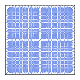
Figure 1.1. Modular inverses: $X=600$, $N(X)=109500$.

By (1.3), the average spacing between two points in ${\mathcal{S}}(X)$ is about $1/X$, so most optimistically one might hope to say something about the distribution of points in sets of volume a little larger than $1/X^{2}$. Clearly, for smaller sets we cannot expect any reasonable statistics. However, already for boxes of volume $1/X$ some irregularities occur because under the hyperbola $\{(x,y)\in[0,1)^{2}:\leavevmode\nobreak\ xy<1/X\}$ the only points in ${\mathcal{S}}(X)$ are

(1.7) $$(x,y)=(1/c,1/c),\qquad\sqrt{X}<c\leq X.$$

It follows that

• the box $[0,1]\times[0,1/(2X)]$ contains no point from ${\mathcal{S}}(X)$;

• the box $[2/\sqrt{X},3/\sqrt{X}]\times[0.2/\sqrt{X},0.25/\sqrt{X}]$ contains no point from ${\mathcal{S}}(X)$;

• the box $[0,1/\sqrt{X}]\times[0,1/\sqrt{X}]$ contains exactly the $(1+o(1))X$ points (1.7) while by (1.3) the expected value is only $(3/\pi^{2}+o(1))X$.

Similar phenomena occur at other rational points with small denominators.

From this discussion we conclude the following:

• The smallest distance between two points in ${\mathcal{S}}(X)$ is of size $1/X^{2}$, namely between the points

  $$(1/[X],1/[X])\quad\text{and}\quad(1/([X]-1),1/([X]-1)).$$

• There are discs of radius $r\gg 1/\sqrt{X}$ without points in ${\mathcal{S}}(X)$.

1.3. Discrepancy

1.3.1. General definitions

An important quantity when studying the distribution of a finite set $S$ in some ambient space ${\mathcal{T}}$ is the discrepancy. Let ${\mathcal{A}}$ be a set of measurable subsets of ${\mathcal{T}}$. Then the discrepancy $\Delta(S,{\mathcal{A}})$ of $S$ with respect to ${\mathcal{A}}$ is

$$\Delta(S,{\mathcal{A}})=\underset{A\in{\mathcal{A}}}{\sup}\left|\frac{\#(S\cap A)}{\#S}-\mu(A)\right|.$$

If $S={\mathcal{S}}(X)$, we write $\Delta(X,{\mathcal{A}})$ instead of $\Delta({\mathcal{S}}(X),{\mathcal{A}})$ for notational simplicity.

Typical choices for ${\mathcal{A}}$ are the subset of boxes or the subset of balls or the subset of convex sets of ${\mathcal{T}}$. With this in mind let ${\mathcal{B}}$ be the set of boxes

(1.8) $$B=[\xi,\xi+\alpha]\times[\zeta,\zeta+\beta]\subseteq\left({\mathbb{R}}/{\mathbb{Z}}\right)^{2}$$

with $0\leq\alpha,\beta<1$, let ${\mathcal{D}}$ be the set of (injective) discs

(1.9) $$D=\{\bm{\xi}:\leavevmode\nobreak\ \|\bm{\xi}-\bm{\omega}\|<R\}\subseteq\left({\mathbb{R}}/{\mathbb{Z}}\right)^{2}$$

for $0\leq R<1/2$, and let ${\mathcal{C}}$ the set of convex subsets in

$$\mathrm{U}=[0,1)^{2},$$

which we identify with $\left({\mathbb{R}}/{\mathbb{Z}}\right)^{2}$. The discrepancy with respect to convex sets is often called isotropic discrepancy. We refer to [11, 23] for historical background on isotropic discrepancy.

In the framework of empirical processes indexed by sets, one would expect that the discrepancy of random point sets with respect to any reasonable class of test sets ${\mathcal{A}}$ satisfies the law of iterated logarithm, in particular

(1.10) $$\limsup_{\#S\rightarrow\infty}\left(\Delta(S,{\mathcal{A}})\frac{\sqrt{\#S}}{\sqrt{2\log\log\#S}}\right)=\frac{1}{2}\quad\text{almost surely}.$$

In particular this holds for the isotropic discrepancy of random point sets in $\left({\mathbb{R}}/{\mathbb{Z}}\right)^{2}$; cf. Philipp [28, Section 3].

Available techniques, however, are very sensitive to the class of test sets. For instance, by a special (and somewhat crude) form of the result of Schmidt [31, Theorem 2], we have

(1.11) $$\Delta(X,{\mathcal{C}})\ll\Delta(X,{\mathcal{B}})^{1/2}.$$

(see also [23, Chapter 2, Theorem 1.6]).

1.3.2. Lower bounds

From the end of Section 1.2 we conclude

(1.12) $$\Delta(X,{\mathcal{B}})\gg 1/X\qquad\mbox{and}\qquad\Delta(X,{\mathcal{D}})\gg 1/X.$$

A slightly sharper lower bound can be obtained for $\Delta(X,{\mathcal{C}})$.

Theorem 1.3.

We have

$$\Delta(X,{\mathcal{C}})\gg\frac{\log X}{X}.$$

Proof.

We observe that there are $O(X)$ points from ${\mathcal{S}}(X)$ under the hyperbola $\{(x,y)\in\mathrm{U}^{2}:\leavevmode\nobreak\ xy<1/X\}$. Therefore, the convex domain $\left\{(x,y)\in\mathrm{U}^{2}:\leavevmode\nobreak\ xy\geq 1/X\right\}$ contains $N(X)+O(X)$ points from ${\mathcal{S}}(X)$, while its area is $1-X^{-1}\log X+O\left(X^{-1}\right)$. We conclude that

$$\Delta(X,{\mathcal{C}})\geq\left|\frac{N(X)+O(X)}{N(X)}-1+\frac{\log X+O(1)}{X}\right|=\frac{\log X+O(1)}{X},$$

which in fact is a little stronger than the claimed bound. ∎

Remark 1.4.

We emphasize that the lower bound in Theorem 1.3 is slightly larger than what we would expect with probability one from a random point set by (1.10). In particular, the set ${\mathcal{S}}(X)$ has some arithmetic structures that, at least on a small scale, lead to deviations from randomness. We refer again to Figure 1.1 whose distinctive cellular structure appears to be shaped by underlying arithmetic properties; the cells sit between lines with rational coordinates with small denominators. See also [4] and [13] for such deviations in slightly different arithmetic contexts.

1.3.3. Upper bounds

The bound (1.11) indicates that our techniques to analyze the discrepancy are quite sensitive to the choice of ${\mathcal{A}}$, which becomes in particular apparent if Fourier-analytic methods are applied: in this case the bounds depend on regularity properties of the Fourier transform of the characteristic functions of $A\in{\mathcal{A}}$. The Fourier transform of boxes is in the $\ell^{1+\varepsilon}$-space for any fixed $\varepsilon>0$, which leads to fairly strong bounds. The Fourier transform of two-dimensional balls is only in the $\ell^{4/3+\varepsilon}$-space; cf. [16, Equations (2.3) and (2.6)]), so one may expect slightly weaker bounds in this case. For general convex sets we have much less control on the Fourier transform of the corresponding characteristic functions, and we study the isotropic discrepancy by an approximation argument to be described later.

Theorem 1.5.

We have

$$\Delta(X,{\mathcal{B}})\leq X^{-5/6+o(1)},$$

as $X\to\infty$.

The exponent $-5/6$ in Theorem 1.5 is an artefact of sharp cut-off $c\leq X$ in the definition (1.2) of ${\mathcal{S}}(X)$. If we study a “weighted discrepancy”, which includes a smooth weight $W(c/X)$, our argument gives the essentially best possible bound $\Delta_{\text{smooth}}(X,{\mathcal{B}})\leq X^{-1+o(1)}$. The same bound would follow also for sharp cut-offs from the modified Selberg–Linnik conjecture (1.6), which we reiterate is out of reach with current technology.

For small boxes we can refine Theorem 1.5 using techniques of Barton, Montgomery and Vaaler [2] (see Lemma 2.2 below) which appear to be less known than they deserve.

Theorem 1.6.

For a box $B$ as in (1.8) such that

(1.13) $$\mu(B)>X^{-1}$$

we have

$$\left|\frac{\#(B\cap{\mathcal{S}}(X))}{N(X)}-\mu(B)\right|\leq\mu(B)^{2/3}X^{-1/3+o(1)},$$

as $X\to\infty$.

Theorem 1.6 improves Theorem 1.5 for $\mu(B)<X^{-3/4+\varepsilon}$, while for large boxes $B$, Theorem 1.5 is more precise.

The condition (1.13) is introduced so that our argument reaches its maximal strength. Our argument continues to work beyond the restrictions (1.13) and still produces nontrivial results. On the other hand, as we saw above, general statements about boxes of volume below $1/X$ are only of restricted relevance.

Combining our Theorem 1.1 with the ideas of Humphries [16] we derive the following bound for the distribution in discs.

Theorem 1.7.

For a disc $D$ as in (1.9) of radius $R<1/2$ we have

$$\left|\frac{\#(D\cap{\mathcal{S}}(X))}{N(X)}-\pi R^{2}\right|\leq(X^{-1}+R^{2/3}X^{-2/3})X^{o(1)},$$

as $X\to\infty$.

The term $R^{2/3}X^{-2/3}$ in the bound of Theorem 1.7 is less than the main term $\pi R^{2}$ as long as $R>X^{-1/2+o(1)}$. We see from Theorem 1.7 that

$$\Delta(X,{\mathcal{D}})\leq X^{-2/3+o(1)}.$$

Turning to the isotropic discrepancy, from (1.11) and Theorem 1.5 we obtain the baseline bound $\Delta(X,{\mathcal{C}})\leq X^{-5/12+o(1)},$ as $X\to\infty$. Using the approach of [19, 20, 35], which in turn exploits some ideas of Schmidt [31, Theorem 2], we establish a stronger bound.

Theorem 1.8.

We have

$$\Delta(X,{\mathcal{C}})\leq X^{-11/24+o(1)},$$

as $X\to\infty$.

2. Preliminaries

2.1. Notation and conventions

For a finite set ${\mathcal{S}}$, we use $\#{\mathcal{S}}$ to denote its cardinality. As usual, the equivalent notations

$$U=O(V)\quad\Longleftrightarrow\quad U\ll V\quad\Longleftrightarrow\quad V\gg U$$

all mean that $|U|\leq CV$ for some positive constant $C$, which, unless indicated otherwise, is absolute. We also write $U=V^{o(1)}$ if, for any given $\varepsilon>0$, there exist $c(\varepsilon)>0$ such that $|U|\leq c(\varepsilon)V^{\varepsilon}$. Furthermore, for two quantities $U$ and $V$, depending on $X,M,N$, we use the notation

$$U\preccurlyeq V\quad\Longleftrightarrow\quad U\ll V(MNX)^{o(1)}.$$

2.2. Point distribution in boxes and exponential sums

For the sake of completeness, we present the auxiliary results in full generality for $d$-dimensional finite sets $S$ in the set ${\mathcal{B}}$ of $d$-dimensional boxes

(2.1) $$B=[\xi_{1},\xi_{1}+\alpha_{1}]\times\ldots\times[\xi_{d},\xi_{d}+\alpha_{d}]\subseteq\left({\mathbb{R}}/{\mathbb{Z}}\right)^{d},$$

of volume $\mu\left(B\right)=\alpha_{1}\cdots\alpha_{d}$. For our application we only need the case $d=2$.

One of the basic tools used to study uniformity of distribution is the celebrated Koksma–Szüsz inequality [22, 37] (see also [11, Theorem 1.21]), which generalises the Erdős–Turán inequality to general dimensions. Like the Erdős–Turán inequality, the Koksma–Szüsz inequality links the discrepancy of a sequence of points to certain exponential sums.

In this section, all implied constants may depend only on the dimension $d$.

Lemma 2.1.

For any integer $M\geq 1$, we have

$$\Delta(S,{\mathcal{B}})\ll\frac{1}{M}+\frac{1}{\#S}\sum_{\begin{subarray}{c}\mathbf{m}\in\mathbb{Z}^{d}\\ 0<\|\mathbf{m}\|\leq M\end{subarray}}\frac{1}{r(\mathbf{m})}\left|\sum_{s\in S}{{e}}{(\langle\mathbf{m},s\rangle)}\right|,$$

where $\langle\mathbf{m},s\rangle$ denotes the inner product in ${\mathbb{R}}^{d}$,

$$\|\mathbf{m}\|=\max_{j=1,\ldots,d}\left|m_{j}\right|\qquad\mbox{and}\qquad r(\mathbf{m})=\prod_{j=1}^{d}\left(\left|m_{j}\right|+1\right).$$

Next we formulate [2, Theorems 1 and 3] which give upper and lower bounds for $\#(S\cap B)$ for individual boxes $B$. To simplify the exposition, we present these bounds without explicit constants and with some other simplifying assumptions.

Lemma 2.2.

Let $S\subseteq\left({\mathbb{R}}/{\mathbb{Z}}\right)^{d}$ be a finite set and let $B$ be a box as in (2.1). Assume that $L_{i}\in{\mathbb{N}}$ satisfies $\alpha_{i}L_{i}\geq 2$ for $i=1,\ldots,d$. Then

$$\#(S\cap B)=\mu\left(B\right)\#S\left(1+O(\max(E,E^{2})\right)$$

where

$$E=\sum_{i=1}^{d}\alpha_{i}^{-1}L_{i}^{-1}+\frac{1}{\#S}\sum_{\begin{subarray}{c}\mathbf{m}\in{\mathcal{L}}\\ \mathbf{m}\neq\mathbf{0}\end{subarray}}\left|\sum_{s\in S}{{e}}\left(\langle\mathbf{m},s\rangle\right)\right|,$$

in which the sum is taken over all non-zero integer vectors $\mathbf{m}$ in the box ${\mathcal{L}}=[-L_{1},L_{1}]\times\cdots\times[-L_{d},L_{d}]$.

Proof.

We first consider the case when there are no points of $S$ on the boundary of $B$, and where

(2.2) $$\alpha_{i}L_{i}\in{\mathbb{N}},\qquad i=1,\ldots,d,$$

to make it closer to the setting of [2, Theorems 1 and 3].

We merely explain deviations from the setting of [2, Theorems 1 and 3]. First we replaced $L_{i}+1$ with $L_{i}$, which means we just add more terms over which we average absolute values of the exponential sums in $E$. Now the lower bound

$$\#(S\cap B)\geq\mu\left(B\right)\#S\left(1+O(E)\right)$$

follows from [2, Theorem 1].

To derive the upper bound for $\#(S\cap B)$ we note that we can assume $\alpha_{i}^{-1}L_{i}^{-1}<1/2$, $i=1,\ldots,d$, as otherwise the result is trivial. Hence, we have the condition [2, Equation (1.10)] with

$$\delta=\prod_{i=1}^{d}(1+\alpha_{i}^{-1}L_{i}^{-1})-1\ll\sum_{i=1}^{d}\alpha_{i}^{-1}L_{i}^{-1}$$

and the bound

$$\#(S\cap B)\leq\mu\left(B\right)\#S\left(1+O(E)\right)$$

follows from [2, Theorem 3]. Hence, under the condition (2.2) we have

(2.3) $$\#(S\cap B)\leq\mu\left(B\right)\#S\left(1+O(E)\right).$$

To drop the condition (2.2), we use a simple approximation argument. We want to construct sets $B^{-}\subseteq B\subseteq B^{+}$ approximating $B$ and satisfying the integrality conditions as in (2.2). We do this as follows: Choose an integer $2\leq b_{i}\leq L_{i}$ such that

$$\frac{b_{i}}{L_{i}}\leq\alpha_{i}<\frac{b_{i}+1}{L_{i}},$$

and define

$$\alpha_{i}^{-}=\frac{b_{i}-1}{L_{i}},\qquad\mbox{and}\qquad\alpha_{i}^{+}=\min\left\{\frac{b_{i}+2}{L_{i}},1\right\}.$$

Then we let

$$B^{\pm}=[\xi_{1}^{\pm},\xi_{1}^{\pm}+\alpha_{1}^{\pm}]\times\ldots\times[\xi_{d}^{\pm},\xi_{d}^{\pm}+\alpha_{d}^{\pm}],$$

where $\xi_{i}^{-}\geq\xi_{i}$, $\xi_{i}^{+}\leq\xi_{i}$ are chosen such that $|\xi_{i}-\xi_{i}^{\pm}|\leq(2L_{i})^{-1}$ and such that the boundary of $B^{\pm}$ contains no points from $S$. Since we only need to avoid finitely many points this is surely possible. Then $B^{-}\subseteq B\subseteq B^{+}$ and the boxes $B^{\pm}$ both satisfy the integrality conditions as in (2.2), with the integers $L_{1},\ldots,L_{d}$. Also, we have $|\alpha_{i}^{+}-\alpha_{i}^{-}|\leq 3/L_{i}$, so

$$|B^{\pm}| =\prod_{i=1}^{d}\left(\alpha_{i}+O(L_{i}^{-1})\right)=\mu\left(B\right)\prod_{i=1}^{d}\left(1+O\left(\frac{1}{\alpha_{i}L_{i}}\right)\right)$$

$$=\mu\left(B\right)\left(1+O\left(\sum_{i=1}^{d}\alpha_{i}^{-1}L_{i}^{-1}\right)\right)=\mu\left(B\right)\left(1+O\left(E\right)\right).$$

Furthermore,

$$\sum_{i=1}^{d}\frac{1}{\alpha_{i}^{\pm}L_{i}}\leq 2\sum_{i=1}^{d}\frac{1}{\alpha_{i}L_{i}},$$

so defining the corresponding quantity $E^{\pm}$ for the approximate boxes $B^{\pm}$, we have $E^{\pm}=O(E)$. Clearly,

$$\#(S\cap B^{-})\leq\#(S\cap B)\leq\#(S\cap B^{+}).$$

Since (2.3) gives

$$\#(S\cap B^{\pm})=|B^{\pm}|\#S\left(1+O(E^{\pm})\right)=\mu\left(B\right)\#S\left(1+O(E)\right)^{2}$$

we get the result. ∎

Remark 2.3.

Clearly, for $E\leq 1$, which is certainly the most interesting case, the error term in the bound of Lemma 2.2 simplifies as $O(E)$. However, it is conceivable that in some scenarios we have $E>1$, in which case it may still be used as an upper bound (rather than a genuine asymptotic formula).

2.3. Point distribution in discs and exponential sums

For the following connection between the number elements of a finite sequence $S\subseteq\left({\mathbb{R}}/{\mathbb{Z}}\right)^{2}$ in a given disc and exponential sums (similar to Lemmas 2.1 and 2.2) we follow Humphries [16], which is formulated for the specific case of the set (1.1), however at the cost of just typographical changes it can be extended to arbitrary sets $S$. Let

$$J_{1}(x)=\sum_{k=0}^{\infty}\frac{(-1)^{l}}{k!(k+1)!2^{2k+1}}x^{2k+1}$$

be the usual Bessel function of index 1. We recall the bound

(2.4) $$J_{1}(x)\ll\min\{x,x^{-1/2}\},$$

which follows from [15, Equation 8.451.1] if $x$ is large enough, and for small $x$ follows directly from the definition.

The following result is essentially a generalised version of [16, Equation (3.1)].

Lemma 2.4.

Let $S\subseteq\left({\mathbb{R}}/{\mathbb{Z}}\right)^{2}$ be a finite set and let $D$ be a disc as in (1.9). Assume that $0<\rho\leq R/2$. Then

$$\pi(R-\rho)^{2}\#S+E_{-}\leq\#(S\cap D)\leq\pi(R+\rho)^{2}\#S+E_{+}$$

where $E_{\pm}$ is given by

$$\frac{R}{\rho}\sum_{\mathbf{u}\in{\mathbb{Z}}^{2}\setminus(0,0)}\frac{J_{1}\left(2\pi(R\pm\rho)\|\mathbf{u}\|_{2}\right)J_{1}\left(2\pi\rho\|\mathbf{u}\|_{2}\right)}{\|\mathbf{u}\|_{2}^{2}}{{e}}\left(-\langle\mathbf{u},\bm{\omega}\rangle\right)\sum_{s\in S}{{e}}\left(\langle\mathbf{u},s\rangle\right)$$

for $\|\mathbf{u}\|_{2}=\sqrt{u_{1}^{2}+u_{2}^{2}}$.

3. Some geometric arguments

3.1. Approximation of well-shaped sets by a union of squares

The following definitions and constructions work in any dimension and are adapted from [31, Section 3] and [20, Section 2]. However, for simplicity we restrict ourselves to dimension $2$.

Let $\|\mathbf{v}\|_{2}$ denote the Euclidean norm of $\mathbf{v}\in{\mathbb{R}}^{2}$, and define the distance between $\mathbf{u}\in{\mathbb{R}}^{2}$ and any $\Omega\subseteq{\mathbb{R}}^{2}$ to be

$$\operatorname{dist}(\mathbf{u},\Omega)=\inf_{\mathbf{w}\in\Omega}\|\mathbf{u}-\mathbf{w}\|_{2}.$$

Let

$$\mathrm{B}=\{\mathbf{v}\in{\mathbb{R}}^{2}:\leavevmode\nobreak\ \|\mathbf{v}\|_{2}\leq 1\}\qquad\mbox{and}\qquad\mathrm{U}=[0,1)^{2}$$

be the closed unit ball and the half-open unit square, respectively. Consider a subset $\Omega\subseteq\mathrm{U}$. For any $\varepsilon>0$ we define the $\varepsilon$-extended set $\Omega_{\varepsilon}$, and the $\varepsilon$-restricted set $\Omega_{-\varepsilon}$ by

$$\Omega_{\varepsilon}=\{\mathbf{u}\in\mathrm{U}:\leavevmode\nobreak\ \operatorname{dist}(\mathbf{u},\Omega)<\varepsilon\},$$

$$\Omega_{-\varepsilon}=\{\mathbf{u}\in\Omega:\leavevmode\nobreak\ \operatorname{dist}(\mathbf{u},\mathrm{U}\backslash\Omega)\geq\varepsilon\}.$$

We then define the sets

$$\Omega_{\varepsilon}^{+}=\Omega_{\varepsilon}\backslash\Omega=\{\mathbf{u}\in\mathrm{U}\backslash\Omega:\leavevmode\nobreak\ \operatorname{dist}(\mathbf{u},\Omega)<\varepsilon\},$$

$$\Omega_{\varepsilon}^{-}=\Omega\backslash\Omega_{-\varepsilon}=\{\mathbf{u}\in\Omega:\leavevmode\nobreak\ \operatorname{dist}(\mathbf{u},\mathrm{U}\backslash\Omega)<\varepsilon\}.$$

The Lebesgue measure of these sets, $\mu(\Omega_{\varepsilon}^{\pm})$, quantifies how much $\Omega$ has been extended or restricted by $\Omega_{\pm\varepsilon}$, respectively. For a given $\eta>0$ we say that a set $\Omega\subseteq\mathrm{U}$ is $\eta$-well-shaped if for all $\varepsilon>0$ we have

$$\mu\left(\Omega_{\varepsilon}^{\pm}\right)\leq\eta\varepsilon.$$

There is another subset of $\Omega$ which is useful. This is defined by

$$\widetilde{\Omega}_{-\varepsilon}=\{\mathbf{u}\in\Omega:\leavevmode\nobreak\ \mathbf{u}+\varepsilon\mathrm{B}\subseteq\Omega\}.$$

One shows that

(3.1) $$\widetilde{\Omega}_{-\varepsilon}\subseteq\Omega_{-\varepsilon}\subseteq\widetilde{\Omega}_{-\varepsilon_{0}}\quad\textrm{ if }0<\varepsilon_{0}<\varepsilon.$$

We now explain how to approximate a well-shaped set $\Omega$ by a union of squares: Fix irrational $\alpha,\beta\in{\mathbb{R}}\backslash{\mathbb{Q}}$. For positive $k$, let ${\mathcal{Q}}(k)$ be the set of squares $\Gamma$ of the form

$$\Gamma_{u,v,k}=\left[\alpha+\frac{u}{k},\alpha+\frac{u+1}{k}\right]\times\left[\beta+\frac{v}{k},\beta+\frac{v+1}{k}\right]\subseteq{\mathbb{R}}^{2},$$

where $u,v\in{\mathbb{Z}}$. The role of the irrationality condition is to ensure that a rational point is always in the interior of the squares in ${\mathcal{Q}}(k)$ and therefore in particular in precisely one square. Furthermore, let

$${\mathcal{Q}}_{\Omega}(k)=\{\Gamma\in{\mathcal{Q}}(k):\leavevmode\nobreak\ \Gamma\subseteq\Omega\}$$

be the set of squares in ${\mathcal{Q}}(k)$ that are contained in $\Omega$. We claim that for any $\varepsilon>\sqrt{2}/k$ we have

(3.2) $$\Omega_{-\varepsilon}\subseteq\widetilde{\Omega}_{-\frac{\sqrt{2}}{k}}\subseteq\bigcup_{\Gamma\in{\mathcal{Q}}_{\Omega}(k)}\Gamma\subseteq\Omega.$$

The first inclusion follows from (3.1). To see that the second inclusion holds, let $\mathbf{x}\in\widetilde{\Omega}_{-\frac{\sqrt{2}}{k}}$, and choose $u_{0},v_{0}\in{\mathbb{Z}}$ such that $\mathbf{x}\in\Gamma_{k,u_{0},v_{0}}$. For $\mathbf{y}\in\Gamma_{k,u_{0},v_{0}}$ we have

$$\|\mathbf{x}-\mathbf{y}\|_{2}\leq\frac{\sqrt{2}}{k},$$

that is, $\mathbf{y}\in\mathbf{x}+\sqrt{2}k^{-1}\mathrm{B}$, so $\mathbf{y}\in\Omega$ since $\mathbf{x}\in\widetilde{\Omega}_{-\sqrt{2}/k}$. This proves that $\Gamma_{k,u_{0},v_{0}}\subseteq\Omega$ so $\Gamma_{k,u_{0},v_{0}}\in{\mathcal{Q}}_{\Omega}(k)$ which shows the second inclusion in (3.2). The third inclusion is clear from the definition of ${\mathcal{Q}}_{\Omega}(k)$.

From (3.2) we find, since $\mu(\Gamma)=k^{-2}$ for $\Gamma\in{\mathcal{Q}}(k)$, that if $\Omega$ is $\eta$-well-shaped, then for any $\delta>0$ we have

(3.3) $$-\eta\frac{(\sqrt{2}+\delta)}{k}+\mu(\Omega)\leq k^{-2}\#{\mathcal{Q}}_{\Omega}(k)\leq\mu(\Omega)$$

and by letting $\delta$ tend to zero the same holds also for $\delta=0$. We now describe how to pack an $\eta$-well-shaped set $\Omega$ with smaller and smaller squares: Let ${\mathcal{B}}_{1}={\mathcal{Q}}_{\Omega}(2)$ and for $i=2,3,\ldots$, let ${\mathcal{B}}_{i}$ be the set of squares $\Gamma\in{\mathcal{Q}}_{\Omega}(2^{i})$ that are not contained in any square from ${\mathcal{Q}}_{\Omega}(2^{i-1})$.

Figure 3.1. $\Omega$ and ${\mathcal{B}}(i)$ in $\mathrm{U}$ for $i\leq 6$

We note that

(3.4) $$\bigcup_{\Gamma\in{\mathcal{Q}}_{\Omega}(2^{n})}\Gamma=\bigcup_{i=1}^{n}\bigcup_{\Gamma\in{\mathcal{B}}_{i}}\Gamma.$$

Using this and (3.2) we see that if $\Omega$ is $\eta$-well-shaped then

$$2^{-2n}\#{\mathcal{B}}_{n}+2^{-2(n-1)}\#{\mathcal{Q}}_{\Omega}(2^{n-1})\leq\mu(\Omega)$$

and combining this with (3.3) we see that

(3.5) $$\#{\mathcal{B}}_{n}\leq\eta 2^{n+3/2}.$$

Using again (3.4) and (3.2) we see also, that if $\Omega$ is $\eta$-well-shaped then

(3.6) $$0\leq\mu(\Omega)-\sum_{i=1}^{n}\sum_{\Gamma\in{\mathcal{B}}_{i}}\mu(\Gamma)\leq\eta 2^{-n+1/2}.$$

3.2. Approximations of convex sets

We now assume that $\Omega\subseteq\mathrm{U}$ is convex. In this case the closure $\overline{\Omega}$, interior $\Omega^{\circ}$, restrictions and extensions $\Omega_{\pm\varepsilon}$, $\widetilde{\Omega}_{-\varepsilon}$ are all convex.

Also recall that the boundary of a convex set has measure zero, see [26, Theorem 1].

Lemma 3.1.

A convex set $\Omega\subseteq\mathrm{U}$ is $(4+\pi)$-well-shaped.

Proof.

A slight variant of this is stated without proof by Schmidt [31, Lemma 1]. We prove it for convex polygons and leave the approximation of general convex sets by convex polygons to the reader (compare [36, Lemma 2.2]). In fact for our application to the isotropic discrepancy it is enough to study only convex polygons, see [23, Chapter 2, Theorem 1.5].

Since $\Omega_{\varepsilon}^{\pm}\subseteq\mathrm{U}$ we have $\mu(\Omega_{\varepsilon}^{\pm})\leq 1\leq(4+\pi)\varepsilon$ if $\varepsilon>1$, so we assume that $\varepsilon\leq 1$.

Given a convex polygon ${\mathcal{P}}$ we can attach a closed rectangle of width $\varepsilon$ to the outside and inside of each side of the polygon.

Figure 3.2. Convex polygon ${\mathcal{P}}$, ${\mathcal{P}}$ with inner rectangles, ${\mathcal{P}}$ with outer rectangles and circular sectors.

For the inside rectangles, convexity of ${\mathcal{P}}$ implies that these overlap and their union covers $\Omega_{\varepsilon}^{-}$.

For the outside we also add a circular sector of radius $\varepsilon$ to each corner of the polygon connecting the two sides of the attached outer rectangles. The restriction to $\mathrm{U}$ of the union of the outer rectangles and the angular sectors covers $\Omega_{\varepsilon}^{+}$. By convexity of ${\mathcal{P}}$ the union of the circular sectors is precisely a full circle of radius $\varepsilon$.

Let $\ell({\mathcal{P}})$ be the length of the perimeter. The above considerations implies that

$$\mu({\mathcal{P}}_{\varepsilon}^{+})\leq\ell({\mathcal{P}})\varepsilon+\pi\varepsilon^{2}\leq\left(\ell({\mathcal{P}})+\pi\right)\varepsilon,$$

$$\mu({\mathcal{P}}_{\varepsilon}^{-})\leq\ell({\mathcal{P}})\varepsilon.$$

Since for convex sets $\Omega_{1}$, $\Omega_{2}$ with $\Omega_{1}\subseteq\Omega_{2}$ we have $\ell(\Omega_{1})\leq\ell(\Omega_{2})$ (see [36]) we can bound $\ell({\mathcal{P}})$ by the length of the perimeter of the largest convex set in $\mathrm{U}$, which is $\mathrm{U}$ itself. Since $\mathrm{U}$ has perimeter length $\ell(\mathrm{U})=4$ and we have assumed $\varepsilon\leq 1$ we find that $\mu(\Omega_{\varepsilon}^{\pm})\leq(4+\pi)\varepsilon$ which gives the result in the case of convex polygons. ∎

4. Bounding the sums of Kloosterman sums

4.1. Preliminary reduction

Using the trivial identity

$$S(m,n;c)=S(-m,-n;c)$$

and partial summation, we see that Theorem 1.1 can be derived from analyzing the following sums of normalised Kloosterman sums:

$$\mathscr{K}^{\pm}(M,N;X)=\sum_{M\leq m<2M}\sum_{N\leq n<2N}\left|\sum_{X\leq c<2X}\frac{1}{c}S(m,\pm n,c)\right|.$$

Proposition 4.1.

We have

$$\mathscr{K}^{\pm}(M,N;X)\preccurlyeq MN+(MN)^{2/3}X^{1/6}.$$

We prove Proposition 4.1 in Section 4.4 after establishing several auxiliary results.

4.2. Analysis

Throughout this section, we always write $s\in{\mathbb{C}}$ as $s=\sigma+it$ with $\sigma,t\in{\mathbb{R}}$. Furthermore, all implied constants in the symbol ‘$\ll$’ may depend on $\sigma$ (but not on $t$), on some constants $A$, $B$ and $C$, on the integer $j$ and on $\varepsilon>0$, wherever applicable.

For $0<\Delta\leq 1/4$, let $W_{\Delta}$ be a smooth function on ${\mathbb{R}}_{>0}={\mathbb{R}}\cap(0,\infty)$with $W_{\Delta}=1$ on $[1,2]$, $\text{supp}(W_{\Delta})\subseteq[1-\Delta,2+\Delta]$ and such that $\|W^{(j)}\|_{\infty}\ll\Delta^{-j}$ for all $j\in{\mathbb{N}}\cup\{0\}$ (we recall that the implied constant may depend on $j$). One shows, using integration by parts and elementary estimates, that the Mellin transform

(4.1) $$\widehat{W}_{\Delta}(s)=\int_{0}^{\infty}W_{\Delta}(x)x^{s}\frac{dx}{x}$$

of $W_{\Delta}$ is entire and satisfies

(4.2) $$\widehat{W}_{\Delta}(s)\ll\frac{1}{1+|s|}\left(1+|s|\Delta\right)^{-A}$$

for every $A>0$. The key point is that $\widehat{W}_{\Delta}$ has almost uniformly bounded $L^{1}$-norm on fixed vertical strips.

Let

(4.3) $${\mathcal{S}}^{+}=i{\mathbb{R}}\cup\left({\mathbb{N}}-\tfrac{1}{2}\right)\qquad\mbox{and}\qquad{\mathcal{S}}^{-}=i{\mathbb{R}}.$$

For $\varpi\in{\mathcal{S}}^{\pm}$ we define

$${\mathcal{J}}^{\pm}_{\varpi}(x)=\frac{J^{\pm}_{2\varpi}(x)-J^{\pm}_{-2\varpi}(x)}{\sin(\pi\cdot\varpi)},$$

where $J^{+}=J$ is the Bessel-$J$-function, and $J^{-}=I$ is the Bessel-$I$-function. Note that for $\varpi=k-1/2\in{\mathbb{N}}-\tfrac{1}{2}$, we have

$${\mathcal{J}}^{+}_{\varpi}(x)=2(-1)^{k+1}J_{2k-1}(x),$$

and for $\varpi=it\in i{\mathbb{R}}$ we have

$${\mathcal{J}}^{-}_{\varpi}(x)=-\frac{4}{\pi}K_{2it}(x)\cosh(\pi t).$$

We now record the Mellin transforms $\widehat{{\mathcal{J}}}_{\varpi}^{\pm}$ of ${\mathcal{J}}^{\pm}_{\varpi}$ (see, for instance, [15, Equations 6.561.14 and 6.561.16] and also [5, Equation (4.7)])

$$\widehat{{\mathcal{J}}}^{+}_{\varpi}(s)=\begin{cases}\displaystyle{-\frac{2^{s}}{\pi}\Gamma\left(\frac{s}{2}+it\right)\Gamma\left(\frac{s}{2}-it\right)\cos\left(\pi s/2\right)},&\varpi=it,\\ \displaystyle{(-1)^{k+1}2^{s}\frac{\Gamma\left(k-\frac{1}{2}+\frac{s}{2}\right)}{\Gamma\left(k+\frac{1}{2}-\frac{s}{2}\right)}},&\varpi=k-\frac{1}{2},\end{cases}$$

and

$$\widehat{{\mathcal{J}}}^{-}_{\varpi}(s)=-\frac{2^{s}}{\pi}\Gamma\left(\frac{s}{2}+it\right)\Gamma\left(\frac{s}{2}-it\right)\cosh(\pi t),\qquad\varpi=it.$$

For a smooth function with compact support on ${\mathbb{R}}_{>0}$ and $\varpi\in{\mathcal{S}}$ we define

(4.4) $$\widecheck{V}^{\pm}(\varpi)=\int_{0}^{\infty}V(x){\mathcal{J}}^{\pm}_{\varpi}(x)\frac{dx}{x}.$$

Lemma 4.2.

Let $r\in{\mathbb{R}}$, $Z>0$, $\varpi\in{\mathcal{S}}^{\pm}$ and $V$ be a fixed smooth function with compact support in ${\mathbb{R}}_{>0}$. Let

$${\mathcal{I}}^{\pm}(r,\varpi,Z)=\int_{0}^{\infty}V\left(\frac{x}{Z}\right)x^{ir}{\mathcal{J}}^{\pm}_{\varpi}(x)\frac{dx}{x}.$$

Then, for any constant $A>0$,

• if $\varpi=it\in i{\mathbb{R}}$, then

  $${\mathcal{I}}^{\pm} \left(r,it,Z\right)$$

  $$\ll\frac{1}{\left(\left(1+\left||r|-2|t|\right|\right)\left(1+|r|+2|t|\right)\right)^{1/2}}\left(1+\frac{1+\left||r|-2|t|\right|}{1+\frac{Z^{2}}{1+|r|+2|t|}}\right)^{-A};$$

• if $\varpi=k-\tfrac{1}{2}\in{\mathbb{N}}-\tfrac{1}{2}$, then

  $${\mathcal{I}}^{+}\left(r,k-\tfrac{1}{2},Z\right)\ll\frac{1}{k}\left(1+\frac{k}{1+Z}\right)^{-A}.$$

Proof.

By Mellin inversion we have

$${\mathcal{I}}^{\pm}(r,\varpi,Z)=\int_{\sigma+i{\mathbb{R}}}\widehat{{\mathcal{J}}}^{\pm}_{\varpi}(s)\widehat{V}(ir-s)Z^{ir-s}\frac{ds}{2\pi i}$$

for $\sigma>0$. Note that $\widehat{V}$ is entire and rapidly decaying on vertical lines.

In the case $\varpi=k-\tfrac{1}{2}$ we shift the contour to $\sigma=0$ to obtain the bound

$${\mathcal{I}}^{+}(r,k-\tfrac{1}{2},Z) \ll\int_{{\mathbb{R}}}\left|\frac{\Gamma(k-\frac{1}{2}+\frac{i\tau}{2})}{\Gamma(k+\frac{1}{2}-\frac{i\tau}{2})}\right|\left(1+|\tau-r|\right)^{-10}d\tau$$

$$\ll\frac{1}{k}\int_{{\mathbb{R}}}(1+|\tau-r|)^{-10}d\tau\ll\frac{1}{k}.$$

Let $A>0$. If $k\leq A/2+1$, there is nothing else to show. Otherwise, we shift the contour to $\sigma=-A$ without crossing poles, using a bound similar to (4.2), we obtain

$${\mathcal{I}}^{+}\left(r,k-\tfrac{1}{2},Z\right) \ll Z^{A}\int_{{\mathbb{R}}}\left|\frac{\Gamma(k-\frac{1+A}{2}+\frac{i\tau}{2})}{\Gamma(k+\frac{1+A}{2}-\frac{i\tau}{2})}\right|(1+|\tau-r|)^{-10}d\tau$$

$$\ll Z^{A}k^{-1-A}.$$

This completes the proof in the case $\varpi=k-\tfrac{1}{2}$.

In the case $\varpi=it$ we shift the contour to $\sigma=-C\not\in\{0,-2,-4,\ldots\}$ with $C>-1/2$. Then, for any $B>0$, using a bound similar to (4.2) and trivial bounds on $\cos\left(\pi s/2\right)$ and $\cosh(\pi t)$, we see that the corresponding integral $\mathfrak{I}$ along the vertical line $\operatorname{Re}s=-C$ is bounded by

$$\mathfrak{I} \ll Z^{C}\int_{{\mathbb{R}}}\Gamma\left(-\frac{C}{2}+i\left(\frac{\tau}{2}+t\right)\right)\Gamma\left(-\frac{C}{2}+i\left(\frac{\tau}{2}-t\right)\right)$$

$$\qquad\qquad\qquad\qquad\qquad\qquad\times\left(e^{\frac{1}{2}\pi|\tau|}+e^{\pi|t|}\right)\left(1+|\tau-r|\right)^{-B}d\tau$$

$$\quad\ll Z^{C}\int_{{\mathbb{R}}}\left((1+|\tau-2t|)(1+|\tau+2t|)\right)^{-(C+1)/2}(1+|\tau-r|)^{-B}d\tau,$$

where we have used the Stirling asymptotics on the Gamma functions. Since $(1+|\tau\pm 2t|)(1+|\tau-r|)\geq(1+|r\pm 2t|)$, we can further estimate this as

(4.5) $$\begin{split}\mathfrak{I}&\ll Z^{C}((1+|r-2t|)(1+|r+2t|)^{-(C+1)/2}\int_{{\mathbb{R}}}(1+|\tau-r|)^{-(B-C-1)}d\tau\\ &\ll\left(\frac{Z^{2}}{(1+|r-2t|)(1+|r+2t|)}\right)^{C/2}\frac{1}{((1+|r-2t|)(1+|r+2t|))^{1/2}},\end{split}$$

provided that $B\geq C+3$, say.

If $C>0$, then for any $B>0$ we also pick up residues coming from the poles of the Gamma factors. These are bounded by

$$\mathfrak{R} \ll\sum_{\pm}\sum_{n=0}^{[C/2]}\frac{Z^{2n}}{(1+|t|)^{n+1/2}}(1+|r\pm 2t|)^{-B}$$

$$\ll\sum_{\pm}\frac{(1+|r\pm 2t|)^{-B}}{(1+|t|)^{1/2}}\left(1+\frac{Z^{C}}{(1+|t|)^{C/2}}\right).$$

It is easily seen that $(1+4|t|)(1+|r\pm 2t|)\geq(1+|r\mp 2t|)$, so that we have

$$\mathfrak{R} \ll\sum_{\pm}\frac{(1+|r\pm 2t|)^{-(B-\frac{C+1}{2})}}{(1+|r\mp 2t|)^{1/2}}\left(1+\frac{Z^{C}}{(1+|r\mp 2t|)^{C/2}}\right)$$

$$=\sum_{\pm}\frac{(1+|r\pm 2t|)^{-(B-1-\frac{C}{2})}}{((1+|r-2t|)(1+|r+2t|))^{1/2}}\left(1+\frac{Z^{C}}{(1+|r\mp 2t|)^{C/2}}\right).$$

Assuming that $B-1-C/2\geq C/2$ and noting that $\{|r+2t|,|r-2t|\}=\{\left||r|-2|t|\right|,|r|+2|t|\}$, this is yields

$$\mathfrak{R} \ll\frac{1}{((1+|r-2t|)(1+|r+2t|))^{1/2}}$$

$$\qquad\times\left((1+\left||r|-2|t|\right|)^{-D}+\left(\frac{Z^{2}}{(1+||r|-2|t||)(1+|r|+2|t|)}\right)^{D}\right),$$

with $D=C/2$ which then simplifies as

(4.6) $$\mathfrak{R}\ll\frac{1}{((1+|r-2t|)(1+|r+2t|))^{1/2}}\left(\frac{1+\left||r|-2|t|\right|}{1+\frac{Z^{2}}{1+|r|+2|t|}}\right)^{-D}.$$

Thus we write

$${\mathcal{I}}^{\pm}\left(r,it,Z\right)\leq|\mathfrak{I}|+|\mathfrak{R}|$$

and apply (4.5) and (4.6) with $C=2A$, and thus $D=A$ (observe that (4.6) dominates (4.5)), and we apply (4.5) with $C=-1/4$, say (in which case (4.6) is void) to obtain a slightly stronger result than claimed. This completes the proof in the case $\varpi=it$. ∎

4.3. The Kuznetsov formula and the large sieve

We now state the Kuznetsov formula in an abstract form with the large sieve incorporated. Recall the definitions (4.3) and (4.4).

Lemma 4.3.

Let $m,n\in{\mathbb{N}}$ and $V$ a smooth function with compact support on ${\mathbb{R}}_{>0}$. Then there exists a measure $d\mu(\varpi)$ on ${\mathcal{S}}^{\pm}$ and real numbers $\rho_{\varpi}(n),\rho_{\varpi}(m)$ such that

$$\sum_{c=1}^{\infty}\frac{1}{c}S(m,\pm n,c)V\left(4\pi\frac{\sqrt{mn}}{c}\right)=\int_{{\mathcal{S}}^{\pm}}\rho_{\varpi}(m)\rho_{\varpi}(n)\widecheck{V}^{\pm}(\varpi)d\mu(\varpi),$$

where the Hecke relations

(4.7) $$\rho_{\varphi}(m)\rho_{\varpi}(n)=\rho_{\varpi}(1)\sum_{d\mid(m,n)}\rho_{\varpi}\left(\frac{mn}{d^{2}}\right)$$

hold and for any $T,N\geq 1$ and $1\leq H\leq T$, and any sequence $\bm{\alpha}=\left(\alpha(n)\right)_{n=1}^{N}\subseteq{\mathbb{C}}$ we have

$$\int_{T-H\leq|\varpi|\leq T}\left|\sum_{n\leq N}\rho_{\varpi}(n)\alpha(n)\right|^{2}d\mu(\varpi)\ll\left(TH+N\right)^{1+\varepsilon}\|\bm{\alpha}\|_{2}^{2},$$

where $\|\bm{\alpha}\|_{2}$ is the $\ell^{2}$-norm of $\bm{\alpha}$.

The Kuznetsov formula is stated in [17, Theorem 16.5 and 16.6]. The measure $d\mu(\varpi)$ has a discrete part (holomorphic and non-holomorphic cusp forms) and a continuous part (Eisenstein series). Note that for the group $\operatorname{SL}_{2}({\mathbb{Z}})$ there are no exceptional eigenvalues.

The large sieve inequality for $H=T$ is a famous result of Deshouillers and Iwaniec [8], the hybrid form for general $H$ can be found in [18, Theorem 1.1] in the non-holomorphic case. The proof (cf. [18, Equation (3.1)]) shows that it holds automatically for the continuous spectrum. The holomorphic case is similar, and can be found, for instance, in [25].

We quickly derive the following “dual” version of the large sieve.

Lemma 4.4.

In the notation of Lemma 4.3, for any measurable function $f:{\mathcal{S}}\rightarrow{\mathbb{C}}$ we have

$$\sum_{n\leq N}\left|\int_{T-H\leq|\varpi|\leq T}\rho_{\varpi}(n)f(\varpi)d\mu(\varpi)\right|^{2}\ll\left(TH+N\right)^{1+\varepsilon}\int_{T-H\leq|\varpi|\leq T}|f(\varpi)|^{2}d\mu(\varpi).$$

Proof.

Let

$${\mathcal{L}}=\sum_{n\leq N}\left|\int_{T-H\leq|\varpi|\leq T}\rho_{\varpi}(n)f(\varpi)d\mu(\varpi)\right|^{2}=\int_{T-H\leq|\varpi|\leq T}f(\varpi)\sum_{n\leq N}\rho_{\varpi}(n)\alpha_{n}\,d\mu(\varpi),$$

where

$$\alpha_{n}=\int_{t-H\leq|\sigma|\leq T}\overline{f(\sigma)}\rho_{\sigma}(n)\,d\mu(\sigma).$$

By the Cauchy-Schwarz inequality and the large sieve inequality of Lemma 4.3, we obtain

$${\mathcal{L}}^{2}\ll\int_{T-H\leq|\varpi|\leq T}|f(\varpi)|^{2}d\mu(\varpi)\,\cdot\,(TH+N)^{1+\varepsilon}\sum_{n\leq N}|\alpha_{n}|^{2}$$

and since

$$\sum_{n\leq N}|\alpha_{n}|^{2}={\mathcal{L}},$$

the claim now follows. ∎

The next estimate follows immediately from Lemma 4.4 using the function $\varpi\mapsto f(\varpi)\rho_{\omega}(1)$, followed by Lemma 4.3 with $N=1$.

Corollary 4.5.

Let $N,T\geq 1$, $F\geq 0$ and $1\leq H\leq T$. Let $f:{\mathcal{S}}\rightarrow{\mathbb{C}}$ be a measurable function with $|f(\varpi)|\leq F$ for $T-H\leq|\varpi|\leq T$. Then

$$\sum_{n\leq N}\left|\int_{T-H\leq|\varpi|\leq T}\rho_{\varpi}(n)\rho_{\varpi}(1)f(\varpi)d\mu(\varpi)\right|^{2}\ll F^{2}TH\left(TH+N\right)^{1+\varepsilon}.$$

4.4. Proof of Proposition 4.1

We define

$$V_{m,n,\Delta}(x)=W_{\Delta}\left(x\frac{X}{4\pi\sqrt{mn}}\right),$$

where $W_{\Delta}$ is as in (4.2) and the surrounding discussion, and we write

$$\mathscr{K}^{\pm}_{\ast}(M,N;X)=\sum_{M\leq m<2M}\sum_{N\leq n<2N}\left|\sum_{c}\frac{1}{c}S(m,\pm n,c)V_{m,n,\Delta}\left(4\pi\frac{\sqrt{mn}}{c}\right)\right|.$$

We assume generally that $\Delta\geq(MNX)^{-100}$. By the Weil bound (1.5) it is easy to see that

(4.8) $$\begin{split}\mathscr{K}^{\pm}&(M,N;X)-\mathscr{K}^{\pm}_{\ast}(M,N;X)\\ &\preccurlyeq\sum_{M\leq m<2M}\sum_{N\leq n<2N}\gcd(m,n)^{1/2}\Delta X^{1/2}\preccurlyeq MN\Delta X^{1/2}.\end{split}$$

We proceed to estimate $\mathscr{K}^{\pm}_{\ast}(M,N;X)$. To this end, let

$$V(x)=W\left(x\frac{X}{4\pi\sqrt{MN}}\right),$$

where $W$ is a fixed smooth function with support in $[1/100,100]$ and $W(x)=1$ on $[1/50,50]$. We insert this as a redundant factor and write

$$\mathscr{K}^{\pm}_{\ast} (M,N;X)$$

$$=\sum_{M\leq m<2M}\sum_{N\leq n<2N}\left|\sum_{c=1}^{\infty}\frac{1}{c}S(m,\pm n,c)V_{m,n,\Delta}\left(4\pi\frac{\sqrt{mn}}{c}\right)V\left(4\pi\frac{\sqrt{mn}}{c}\right)\right|.$$

The inner sum is in shape to apply the Kuznetzov formula given by Lemma 4.3, along with the Hecke relations (4.7), and we obtain

$$\mathscr{K}^{\pm}_{\ast} (M,N;X)$$

$$\leq\sum_{M\leq m<2M}\sum_{N\leq n<2N}\sum_{d\mid\gcd(m,n)}\left|\int_{{\mathcal{S}}^{\pm}}\rho_{\varpi}(1)\rho_{\varpi}\left(\frac{mn}{d^{2}}\right)\widecheck{(V_{m,n,\Delta}V)}^{\pm}(\varpi)d\mu(\varpi)\right|.$$

We denote

$$U(r,\varpi)^{\pm}=\int_{0}^{\infty}V(x)x^{ir}{\mathcal{J}}^{\pm}_{\varpi}(x)\frac{dx}{x}$$

and Mellin-invert $V_{m,n,\Delta}$, getting

$$\mathscr{K}^{\pm}_{\ast}(M,N;X)$$

$$\ll\sum_{M\leq m<2M}\sum_{N\leq n<2N}\sum_{d\mid\gcd(m,n)}\int_{{\mathbb{R}}}\frac{(1+|r|\Delta)^{-10}}{1+|r|}\left|\int_{{\mathcal{S}}^{\pm}}\rho_{\varpi}(1)\rho_{\varpi}\left(\frac{mn}{d^{2}}\right)U(r,\varpi)^{\pm}d\mu(\varpi)\right|dr$$

$$\leq\sum_{d\leq 2\min\{M,N\}}\sum_{K_{d}\leq\kappa\leq 4K_{d}}\tau(\kappa)\int_{{\mathbb{R}}}\frac{(1+|r|\Delta)^{-10}}{1+|r|}\left|\int_{{\mathcal{S}}^{\pm}}\rho_{\varpi}(1)\rho_{\varpi}(\kappa)U(r,\varpi)^{\pm}d\mu(\varpi)\right|dr$$

where $K_{d}=MN/d^{2}$. We split the set ${\mathcal{S}}^{\pm}$ into countably many pieces

$${\mathcal{S}}^{\pm}=\bigcup_{j=1}^{\infty}{\mathcal{S}}^{\pm}_{j}$$

according to the size of $\varpi$, to be described in a moment. By the Cauchy-Schwarz inequality, we obtain

(4.9) $$\mathscr{K}^{\pm}_{\ast}(M,N;X)\preccurlyeq\sum_{d\leq 2\min\{M,N\}}K_{d}^{1/2}\int_{{\mathbb{R}}}\frac{(1+|r|\Delta)^{-10}}{1+|r|}\Sigma_{d}^{\pm}(r)dr,$$

where

$$\Sigma_{d}^{\pm}(r)=\sum_{j=1}^{\infty}\left(\sum_{K_{d}\leq\kappa\leq 4K_{d}}\left|\int_{{\mathcal{S}}^{\pm}_{j}}\rho_{\varpi}(1)\rho_{\varpi}(\kappa)U(r,\varpi)^{\pm}d\mu(\varpi)\right|^{2}\right)^{1/2}.$$

The innermost $\kappa$-sum is in shape for an application of Corollary 4.5. The integral transform $U(r,\varpi)^{\pm}$ has been estimated in Lemma 4.2, and accordingly we distinguish the cases

$$\varpi=k-\tfrac{1}{2}\in{\mathbb{N}}-\tfrac{1}{2}\qquad\mbox{and}\qquad\varpi=it\in i{\mathbb{R}}.$$

We start with the case $\varpi=k-\tfrac{1}{2}$ and split into dyadic ranges $T_{\nu}\leq k<2T_{\nu}$, where $T_{\nu}=2^{\nu}$, $\nu=0,1,\ldots$, Using Lemma 4.2 with $A=10$ and $Z=\sqrt{MN}/X$ and Corollary 4.5 with $T/2=H=T_{\nu}$ and

$$F\ll\frac{1}{T_{\nu}}\frac{1}{(1+T_{\nu}/(\sqrt{MN}/X))^{10}},$$

we bound, up to $(TMN)^{o(1)}$, this portion of $\Sigma_{d}^{+}(r)$ by

$$\sum_{\nu=0}^{\infty}\left(\frac{1}{T_{\nu}^{2}}\left(1+\frac{T_{\nu}}{\sqrt{MN}/X}\right)^{-20}T_{\nu}^{2}(T_{\nu}^{2}+K_{d})\right)^{1/2}\preccurlyeq\left(\frac{\sqrt{MN}}{X}+\sqrt{MN}\right)\ll\sqrt{MN}.$$

Next we consider the case $\varpi=it\in i{\mathbb{R}}$ using again Lemma 4.2 with $Z=\sqrt{MN}/X$. We split into smaller windows $H_{\nu}\leq 1+\left||r|-2|t|\right|<2H_{\nu}$ where

$$H_{\nu}=2^{\nu}\qquad\mbox{and}\qquad T_{\nu}=H_{\nu}+|r|,\qquad\nu=0,1,\ldots.$$

One shows that in this region we have

$$t\leq T_{\nu}\qquad\mbox{and}\qquad 1/(1+|r|+|2t|)\leq 2/T_{\nu}$$

and that the set of $t$ satisfying these conditions is contained in the union of at most 4 windows of size at most $H_{\nu}$. With $Z=\sqrt{MN}/X$ and

$$F\ll\frac{1}{(T_{v}H_{v})^{1/2}}\left(1+\frac{H_{\nu}}{1+2Z^{2}/T_{\nu}}\right)^{-10}$$

we bound as before (and again up to $(TMN)^{o(1)}$) this portion of $\Sigma_{d}^{\pm}(r)$ by

$$\sum_{\nu=0}^{\infty} \left(\frac{1}{T_{\nu}H_{\nu}}\left(1+\frac{H_{\nu}}{1+Z^{2}/T_{\nu}}\right)^{-20}T_{\nu}H_{\nu}(T_{\nu}H_{\nu}+K_{d})\right)^{1/2}$$

$$\ll\sum_{\nu=0}^{\infty}\left(1+\frac{H_{\nu}}{1+Z^{2}/(H_{\nu}+|r|)}\right)^{-10}\left((H_{\nu}+|r|)H_{\nu}+MN\right)^{1/2}$$

$$\preccurlyeq\left(1+|r|^{1/2+\varepsilon}+Z+(MN)^{1/2}\right)\ll\left(1+|r|^{1/2+\varepsilon}+(MN)^{1/2}\right).$$

We substitute the previous two bounds back into (4.9) getting

$$\mathscr{K}^{\pm}_{\ast}(M,N;X) \preccurlyeq(MN)^{1/2}\int_{{\mathbb{R}}}\frac{\left(1+|r|\Delta\right)^{-10}}{1+|r|}(1+|r|^{1/2+\varepsilon}+(MN)^{1/2})dr$$

$$\preccurlyeq MN+(MN)^{1/2}\Delta^{-1/2}.$$

Together with (4.8) we finally obtain

$$\mathscr{K}^{\pm}(M,N;X)\preccurlyeq MN+MN\Delta X^{1/2}+\frac{\sqrt{MN}}{\Delta^{1/2}}\\ \ll MN+(MN)^{2/3}X^{1/6}$$

upon choosing $\Delta=(MNX)^{-1/3}$, which balances the two last terms. This finishes the proof of Proposition 4.1 and thus of Theorem 1.1.

5. Bounding the uniformity of distribution measures

5.1. Proof of Theorem 1.5

From (1.3) and Lemma 2.1 we see, using a dyadic decomposition, that for any integer $1\leq\ell\ll\log X$ we have

(5.1) $$\Delta(X,{\mathcal{B}})\ll 2^{-\ell}+\frac{1}{X^{2}}\left(S_{*}+S_{0}\right),$$

where

$$S_{*}=\sum_{i,j=0}^{\ell}{\mathcal{K}}(2^{i},2^{j},X)2^{-i-j}\qquad\mbox{and}\qquad S_{0}=\sum_{i=0}^{\ell}\sum_{2^{i}\leq m<2^{i+1}}\left|\sum_{1\leq c\leq X}S(0,m;c)\right|2^{-i}.$$

By Theorem 1.1 and Remark 1.2 we have

$$\Delta(X,{\mathcal{B}})\preccurlyeq 2^{-\ell}+X^{-2}(\ell^{2}X+X^{7/6}).$$

Taking $\ell=\left\lceil\log X/\log 2\right\rceil$ in (5.1) we conclude the proof of Theorem 1.5.

5.2. Proof of Theorem 1.6

We choose two parameters $M,N\in\mathbb{N}$ such that

(5.2) $$\alpha M,\beta N\geq 2,$$

where $\alpha$ and $\beta$ are the side lengths of the box $B$ as in (1.8).

It follows from Theorem 1.1 (and Remark 1.2), equation (1.3) and Lemma 2.2 that

$$\#(B\cap{\mathcal{S}}(X))=\mu\left(B\right)N(X)\left(1+O(E)\right),$$

where

(5.3) $$E\preccurlyeq\alpha^{-1}M^{-1}+\beta^{-1}N^{-1}+MNX^{-1}+(MN)^{2/3}X^{-5/6}.$$

We balance the first two terms and choose $N=\left\lceil\alpha\beta^{-1}M\right\rceil$. We observe that to satisfy (5.2) we now only need to request $\alpha M\geq 2$.

We can certainly assume that $M,N\leq X^{2}$ as otherwise the result is trivial. Hence we see from (5.3) that

$$\Delta\preccurlyeq\alpha^{-1}M^{-1}+\alpha\beta^{-1}M^{2}X^{-1}+\left(\alpha\beta^{-1}\right)^{2/3}M^{4/3}X^{-5/6}.$$

Clearly the above expression minimises at one of the two values of $M$ balancing the first and either the second or the third term. That is, at

$$M_{1}=\left\lceil 2\alpha^{-2/3}\beta^{1/3}X^{1/3}\right\rceil,$$

or at

$$M_{2}=\left\lceil 2\alpha^{-5/7}\beta^{2/7}X^{5/14}\right\rceil.$$

Choosing $M=M_{1}$ leads to the bound

$$\Delta \preccurlyeq\alpha^{-1}M_{1}^{-1}+\left(\alpha\beta^{-1}\right)^{2/3}M_{1}^{4/3}X^{-5/6}$$

$$\ll\mu\left(B\right)^{-1/3}X^{-1/3}+\mu\left(B\right)^{-2/9}X^{-7/18}.$$

We easily verify that for $\mu\left(B\right)\leq 1\leq X$ the first term dominates the second, which finishes the proof of Theorem 1.6.

5.3. Proof of Theorem 1.7

Using Lemma 2.4 and the bound (2.4), we conclude that for any positive $0<\rho\leq R<1/2$ we have

(5.4) $$\left|\#(D\cap{\mathcal{S}}(X))-\pi R^{2}N(X)\right|\ll R\rho N(X)+E_{1}+E_{2}+E_{3},$$

where

$$E_{1}=R^{2}\sum_{\begin{subarray}{c}(m,n)\in{\mathbb{Z}}^{2}\\ 0<m^{2}+n^{2}\leq 1/R^{2}\end{subarray}}\left|\sum_{1\leq c\leq X}S(m,n;c)\right|,$$

$$E_{2}=R^{1/2}\sum_{\begin{subarray}{c}(m,n)\in{\mathbb{Z}}^{2}\\ 1/R^{2}<m^{2}+n^{2}\leq 1/\rho^{2}\end{subarray}}\frac{1}{\left(m^{2}+n^{2}\right)^{3/4}}\left|\sum_{1\leq c\leq X}S(m,n;c)\right|,$$

$$E_{3}=\frac{R^{1/2}}{\rho^{3/2}}\sum_{\begin{subarray}{c}(m,n)\in{\mathbb{Z}}^{2}\\ 1/\rho^{2}<m^{2}+n^{2}\end{subarray}}\frac{1}{\left(m^{2}+n^{2}\right)^{3/2}}\left|\sum_{1\leq c\leq X}S(m,n;c)\right|.$$

We cover the range of summation in each of the above sums by overlapping dyadic intervals with $M\leq|m|\leq 2M$ and $N\leq|n|\leq 2N$, where non-zero values of $M$ and $N$ run through powers of $2$, and we can always assume $M\geq N$.

For $N=0$ we use Remark 1.2 (which gives a negligible contribution to each of the error terms $E_{i}$, $i=1,2,3$ and we do not discuss it below). For $N\geq 1$ use Theorem 1.1, and in fact sometimes it is convenient to use the bound in a weaker form

$${\mathcal{K}}(M,N;X)\leq\left(\left(M^{2}+N^{2}\right)X+\left(M^{2}+N^{2}\right)^{2/3}X^{7/6}\right)(MNX)^{o(1)}.$$

Hence, for $N\geq 1$ each of such sums over dyadic intervals, which are relevant to $E_{1}$, can be estimated as $\left(R^{-2}X+R^{-4/3}X^{7/6}\right)X^{o(1)}$ (where we have also recalled that $R^{-1}\leq X$). Then we immediately derive

(5.5) $$E_{1}\preccurlyeq X+R^{2/3}X^{7/6}.$$

For $E_{2}$, dyadic sums (as before with $N\geq 1$) can be estimated as

$$\frac{{\mathcal{K}}(M,N;X)}{\left(M^{2}+N^{2}\right)^{3/4}} \preccurlyeq\left(M^{2}+N^{2}\right)^{1/4}X+\left(M^{2}+N^{2}\right)^{-1/12}X^{7/6}$$

$$\ll\rho^{-1/2}X+R^{-1/6}X^{7/6}$$

(provided that $\rho\gg X^{-100}$, say). Therefore, together with the contribution from sums with $N=0$, we obtain

(5.6) $$E_{2}\preccurlyeq R^{1/2}\rho^{-1/2}X+R^{2/3}X^{7/6}.$$

For $E_{3}$, we use the full power of Theorem 1.1 and thus for $M\geq N$ the dyadic sums (again with $N\geq 1$) can be estimated as

$$\frac{{\mathcal{K}}(M,N;X)}{\left(M^{2}+N^{2}\right)^{3/2}} \leq M^{-3}\left(MNX+(MN)^{2/3}X^{7/6}\right)(MNX)^{o(1)}$$

$$\leq\left(M^{2}NX+M^{-7/3}N^{2/3}X^{7/6}\right)(MNX)^{o(1)}.$$

Since $M$ and $N$ both run over powers of $2$ with $2M^{2}\geq M^{2}+N^{2}\geq\rho^{-2}$, summing over geometric progressions, we obtain

(5.7) $$E_{3}\preccurlyeq R^{1/2}{\rho^{-3/2}}\left(\rho X+\rho^{5/3}X^{7/6}\right)=R^{1/2}\rho^{-1/2}X+R^{1/2}\rho^{1/6}X^{7/6}.$$

We see that the term $X$ in (5.5) is dominated by $R^{1/2}\rho^{-1/2}X$ in (5.6), and the term $R^{1/2}\rho^{1/6}X^{7/6}$ in (5.7) is dominated by $R^{2/3}X^{7/6}$ in (5.6). Hence substituting (5.5), (5.6) and (5.7) in (5.4), we obtain

$$\#\left(D\cap{\mathcal{S}}(X)\right)-\pi R^{2}N(X)\preccurlyeq R\rho X^{2}+R^{2/3}X^{7/6}+R^{1/2}\rho^{-1/2}X.$$

We now choose

$$\rho=\frac{1}{2}\min(R,R^{-1/3}X^{-2/3})$$

getting

$$\#\left(D\cap{\mathcal{S}}(X)\right)-\pi R^{2}N(X)\preccurlyeq R^{2/3}X^{4/3}+X$$

as desired.

5.4. Proof of Theorem 1.8

Recall that we say that a set $C\subseteq\left({\mathbb{R}}/{\mathbb{Z}}\right)^{2}$ is convex if there exist a convex set $\Omega\subseteq\mathrm{U}=[0,1)^{2}$ such that $\Omega\bmod{\mathbb{Z}}^{2}=C$. Similarly, given $\eta>0$, we say that $\Delta$ is $\eta$-well-shaped if there exist an $\eta$-well-shaped $\Omega\subseteq\mathrm{U}$ as defined in Section 3.1 satisfying $\Omega\bmod{\mathbb{Z}}^{2}=\Delta$.

For the proof of Theorem 1.8 it is technically easier to establish a more general result for the discrepancy

$$\Delta_{\eta}(X)=\sup_{S,\leavevmode\nobreak\ \eta\text{-well-shaped}}\left|\frac{\#(S\cap{\mathcal{S}}(X))}{N(X)}-\mu(S)\right|$$

with respect to $\eta$-well-shaped sets $S\subseteq\left({\mathbb{R}}/{\mathbb{Z}}\right)^{2}$. This is indeed a more general result since, by Lemma 3.1, any convex set in $\left({\mathbb{R}}/{\mathbb{Z}}\right)^{2}$ is $(4+\pi)$-well-shaped so $\Delta(X,{\mathcal{C}})\leq\Delta_{4+\pi}(X)$.

We show that

(5.8) $$\Delta_{\eta}(X)\preccurlyeq\eta X^{-11/24},$$

uniformly over $\eta$. Clearly if $\eta$ is fixed (like in the above scenario relevant to bounding $\Delta(X,{\mathcal{C}})$), the bound (5.8) simplifies as $\Delta_{\eta}(X)\preccurlyeq X^{-11/24}$. However, for completeness and keeping in mind that there could be other applications to $\eta$-well-shaped sets where $\eta$ may depend on $X$, we derive the result in full generality.

To prove (5.8) we note that for $\Omega\subseteq\mathrm{U}$ we have, by definition, that $(\mathrm{U}\backslash\Omega)_{\varepsilon}^{\pm}=\Omega_{\varepsilon}^{\mp}$, using the notation from Section 3.1. It follows that the complement of an $\eta$-well-shaped set $S\subseteq\left({\mathbb{R}}/{\mathbb{Z}}\right)^{2}$ is again an $\eta$-well-shaped set. We therefore conclude, using $\#(S^{c}\cap{\mathcal{S}}(X))=N(X)-\#(S\cap{\mathcal{S}}(X))$, that in order to establish Theorem 1.8 it is enough to prove a lower bound

(5.9) $$\#(S\cap{\mathcal{S}}(X))\geq\mu(S)N(X)+O\left(\eta X^{37/24+o(1)}\right)$$

for such sets.

We start by approximating an $\eta$-well-shaped set $S$ by boxes in ${\mathcal{B}}_{i}$ as described in Section 3.1, cf.  in particular (3.4). From the third inclusion in (3.2) combined with the fact that rational points are in at most in one of the boxes $B_{i}$ we see that

$$\#(S\cap{\mathcal{S}}(X))\geq\sum_{i=1}^{M}\sum_{\Gamma\in{\mathcal{B}}_{i}}\#(\Gamma\cap{\mathcal{S}}(X)).$$

Here we interpret $\Gamma$ as having been mapped to $\left({\mathbb{R}}/{\mathbb{Z}}\right)^{2}$. We want to apply Theorem 1.5 to the larger of these boxes, and Theorem 1.6 to the smaller ones. We first assume $M\leq\log X/(2\log(2))$ such that ${\mathcal{B}}_{M}$ contains boxes that are allowed in Theorem 1.6. We then choose another positive parameter $L\leq M$ and apply Theorem 1.5 to squares $\Gamma\in{\mathcal{B}}_{i}$ with $i\leq L$ and Theorem 1.6 otherwise. In this way we derive

(5.10) $$\#(S\cap{\mathcal{S}}(X))\geq N(X)\sum_{i=1}^{M}\sum_{\Gamma\in{\mathcal{B}}_{i}}\mu(\Gamma)+O\left(RX^{2+o(1)}\right),$$

where

$$R=\sum_{i\leq L}\#{\mathcal{B}}_{i}X^{-5/6}+\sum_{L<i\leq M}\#{\mathcal{B}}_{i}\left(2^{-2i}\right)^{2/3}X^{-1/3}.$$

Recalling the bound (3.5) on $\#{\mathcal{B}}_{i}$, we see that

(5.11) $$R\ll\eta(2^{L}X^{-5/6}+2^{-L/3}X^{-1/3})$$

Furthermore, by (3.6) we have

(5.12) $$\sum_{i=1}^{M}\sum_{\Gamma\in{\mathcal{B}}_{i}}\mu(\Gamma)=\mu(S)+O\left(\eta 2^{-M}\right).$$

Putting these estimates together in (5.10) we find

$$\#(S\cap{\mathcal{S}}(X))\geq N(X)\mu(S)+O(\eta X^{2+o(1)}(2^{L}X^{-5/6}+2^{{-L/3}}X^{-1/3}+2^{-M})).$$

We balance the two first terms and choose

$$L=\left\lfloor\frac{3\log X}{8\log 2}\right\rfloor.$$

Then these two terms are of order $X^{37/24+o(1)}$. Choosing $M$ to satisfy

$$\frac{11\log X}{24\log 2}\leq M\leq\frac{\log X}{2\log 2},$$

we see with this choice $L<M$ and $X^{2}/2^{M}$ is bounded by $X^{37/24+o(1)}$. This gives the desired lower bound (5.9), and therefore concludes the proof of (5.8).

References

• [1] S. Baier, ‘Multiplicative inverses in short intervals’, Int. J. Number Theory 9 (2013), 877–884.
• [2] J. T. Barton, H. L. Montgomery and J. D. Vaaler, ‘Note on a Diophantine inequality in several variables’, Proc. Amer. Math. Soc. 129 (2001), 337–345.
• [3] S. Bettin and V. Chandee, ‘Trilinear forms with Kloosterman fractions’, Adv. Math. 328 (2018), 1234–1262.
• [4] V. Blomer, J. Bourgain, M. Radziwill and Z. Rudnick, ‘Small gaps in the spectrum of the rectangular billiard], Ann. Sci. Ecole Norm. Sup. 50 (2017), 1283–1300
• [5] V. Blomer and J. Buttcane, ‘On the subconvexity problem for $L$-functions on $\operatorname{GL}(3)$’, Ann. Sci. Ecole Norm. Sup. 53 (2020), 1441–1500.
• [6] T. D. Browning and A. Haynes, ‘Incomplete Kloosterman sums and multiplicative inverses in short intervals’, Int. J. Number Theory 9 (2013), 481–486.
• [7] T. H. Chan, ‘Shortest distance in modular hyperbola and least quadratic non-residue’, Mathematika 62 (2016), 860–865.
• [8] J.-M. Deshouillers and H. Iwaniec. ‘Kloosterman sums and Fourier coefficients of cusp forms’, Invent. Math. 70, (1982/83), 219–288.
• [9] E. I. Dinaburg and Y. G. Sinai, ‘The statistics of the solutions of the integer equation $ax-by=\pm 1$’, Funct. Anal. Appl. 24 (1990), 165–171.
• [10] D. Dolgopyat, ‘On the distribution of the minimal solution of a linear Diophantine equation with random coefficients’, Funct. Anal. Appl. 28 (1994), 168–177.
• [11] M. Drmota and R. F. Tichy, Sequences, discrepancies and applications, Springer-Verlag, Berlin, 1997.
• [12] A. Fujii, ‘On a problem of Dinaburg and Sinai’, Proc. Japan Acad. Sci., Ser.A 68 (1992), 198–203.
• [13] M. Z. Garaev and I. E. Shparlinski, ‘On the distribution of modular inverses from short intervals’, Mathematika 69 (2023), 1183–1194.
• [14] A. Good, Local analysis of Selberg’s trace formula, Lecture Notes in Math., Vol. 1040, Berlin, Springer-Verlag, 1983.
• [15] I. S. Gradshteyn and I. M. Ryzhik, Table of integrals, series, and products, Academic Press, 2000.
• [16] P. Humphries, ‘Distributing points on the torus via modular inverses’, Quart J. Math. 73 (2022), 1–16.
• [17] H. Iwaniec and E. Kowalski, Analytic number theory, Amer. Math. Soc., Providence, RI, 2004.
• [18] M. Jutila, ‘On the spectral large sieve inequalities’, Funct. Approx. 28 (2000), 7–18.
• [19] B. Kerr, ‘Solutions to polynomial congruences in well shaped sets’, Bull. Aust. Math. Soc. 88 (2013), 435–447.
• [20] B. Kerr and I. E. Shparlinski, ‘On the distribution of values and zeros of polynomial systems over arbitrary sets’, J. Number Theory 133 (2013), 2863–2873.
• [21] E. M. Kiral, ‘Opposite-sign Kloosterman sum zeta function’, Mathematika 62 (2016), 406–429.
• [22] J. F. Koksma, ‘Some theorems on Diophantine inequalities’, Math. Centrum Scriptum no. 5, Amsterdam, 1950.
• [23] L. Kuipers and H. Niederreiter, Uniform distribution of sequences, Wiley-Intersci., New York-London-Sydney, 1974.
• [24] N. V. Kuznetsov, ‘The Petersson conjecture for cusp forms of weight zero and the Linnik conjecture. Sums of Kloosterman sums’, Math. USSR-Sb. 39 (1981), 299–342 (translated from Matemat. Sbornik 111(153) (1980), 334–383).
• [25] J. Lam, ‘A local large sieve inequality for cusp forms’, J. Théorie Nombres Bordeaux 26 (2014), 757–787.
• [26] R. Lang, ‘A note on the measurability of convex sets’, Archiv Math. 47 (1986), 90–92.
• [27] H.-Q. Liu, ’On Euler’s function’, Proc. Royal Soc. Edinburgh, Sec. A. Math. 146 (2016), 769–775.
• [28] W. Philipp, ‘Empirical distribution functions and uniform distribution mod 1’, Diophantine Approx. and Its Appl., Academic Press, New York–London, 1973, 211–234.
• [29] G. J. Rieger, ‘Über die Gleichung $ad-bc=1$ und Gleichverteilung’, Math. Nachr. 162 (1993), 139–143.
• [30] P. Sarnak and J. Tsimerman, ‘On Linnik and Selberg’s conjectures about sums of Kloosterman sums’, Algebra, Arithmetic, and Geometry, Vol. II: In Honor of Yu. I. Manin, Progress in Math. 270., Boston, Birkhäuser, 2009.
• [31] W. Schmidt, ‘Irregularities of distribution. IX’, Acta Arith. 27 (1975), 385–396.
• [32] A. Selberg, ’Equidistribution in discrete groups and the spectral theory of automorphic forms’, available at http://Publications.IAS.Edu/Selberg/Section/2491, 1977, 25 pages.
• [33] I. E. Shparlinski, ‘On the distribution of solutions to linear equations’, Glasnik Math. 44 (2009), 7–10.
• [34] I. E. Shparlinski, ‘Modular hyperbolas’, Jpn. J. Math. 7 (2012), 235–294.
• [35] I. E. Shparlinski, ‘On the distribution of solutions to polynomial congruences’, Archiv Math. 99 (2012), 345–351.
• [36] G. Stefani, ‘On the monotonicity of perimeter of convex bodies’, J. Convex Analysis 25 (2018), 93–102.
• [37] P. Szüsz, ‘On a problem in the theory of uniform distribution’, Comptes Rendus Premier Congrès Hongrois, Budapest, 1952, 461–472 (in Hungarian).
• [38] A. V. Ustinov, ‘On points of the modular hyperbola under the graph of a linear function’, Math. Notes 97 (2015), 284–288 (translated from Matem. Zametki 97 (2015), 296–301).
• [39] A. Walfisz, ‘Weylsche Exponentialsummen in der neueren Zahlentheorie’, Leipzig: B.G. Teubner, 1963.