From memorization to generalization: a theoretical framework for diffusion-based generative models
Abstract
Diffusion-based generative models demonstrate a transition from memorizing the training dataset to a non-memorization regime as the size of the training set increases. Here, we begin by introducing a mathematically precise definition of this transition in terms of a relative distance: the model is said to be in the non-memorization/‘generalization’ regime if the generated distribution is almost surely far from the probability distribution associated with a Gaussian kernel approximation to the training dataset, relative to the sampling distribution. Then, we develop an analytically tractable diffusion model and establish a lower bound on Kullback–Leibler divergence between generated and sampling distribution. The model also features the transition, according to our definition in terms of the relative distance, when the training data is sampled from an isotropic Gaussian distribution. Further, our study reveals that this transition occurs when the individual distance between the generated and underlying sampling distribution begins to decrease with the addition of more training samples. This is to be contrasted with an alternative scenario, where the model’s memorization performance degrades, but generalization performance doesn’t improve. We also provide empirical evidence indicating that realistic diffusion models exhibit the same alignment of scales.
1 Introduction
In recent years, generative artificial intelligence has made tremendous advancements—be it image, audio, video, or text domains—on an unprecedented scale.222For a discussion of possible impact of machine learning in theoretical sciences see [1, 2]. Diffusion models [3, 4, 5] are among the most successful frameworks, serving as the foundation for prominent content generation tools such as DALL-E [6], Stable Diffusion [7], Imagen [8], Sora [9] and numerous others. However, the factors that contribute to the strong generalization capabilities of diffusion models, as well as the conditions under which they perform optimally, remain open.
In this paper, we will focus on a particular generalization behavior that diffusion models exhibit. Empirical observations show that for a small number of training samples, diffusion models memorize the training data [10, 11]. As the training dataset size increases, they transition from memorizing data to a regime where it can generate new samples [12]. What is the nature of this memorization to non-memorization transition?
In this paper, we take steps toward a better understanding of this phenomenon. Specifically, we provide a mathematically precise definition of the transition in terms of relative distances between the training and generated distribution, denoted as , and the distance between the original underlying distribution and generated distribution, denoted as . We say that the diffusion model is in a non-memorization/‘generalization’ regime if the probability of is very close to unity implying that the generated distribution exhibits greater proximity to the original underlying distribution relative to the training dataset.333Note that our definition does not guarantee if generalization error decreases or increases during the transition that is marked by a change in relative distance .
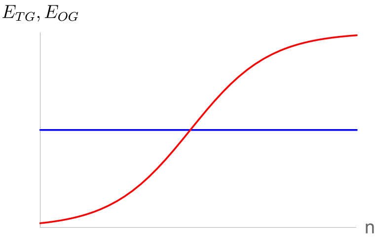
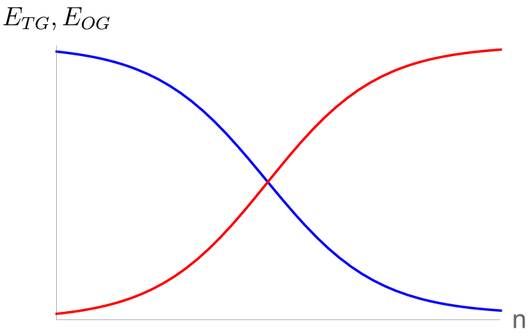
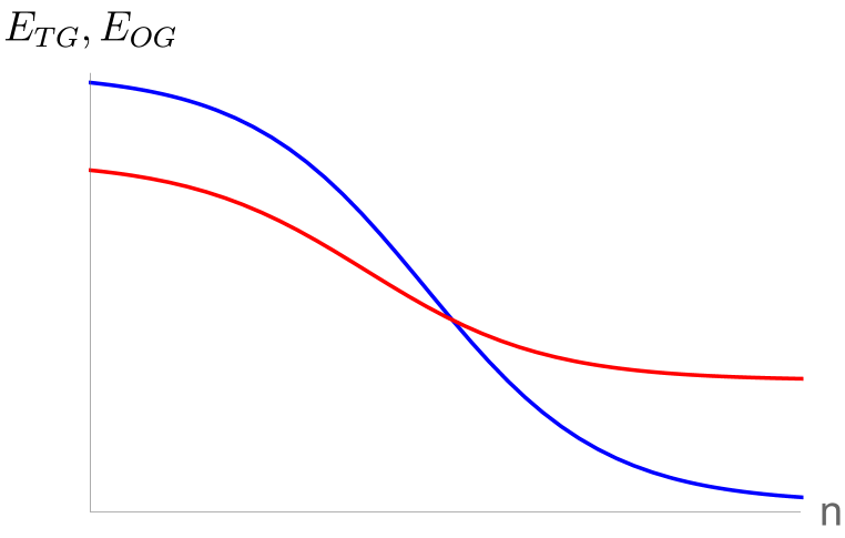
On the onset of memorization to non-memorization transition individually might show very different behaviors as shown in Fig. 1. For example scenario (a) indicates that the model is failing to memorize because of a faster increase in compared to with the increase of train dataset size . However in this case the model does not learn to generalize well because remains almost constant during the transition. The scenarios in (b) and (c) present other possibilities. Empirically, we rule out the possibility (b) in a realistic diffusion model. In this paper, we show that for a diffusion model scenario (c) is the appropriate description, i.e., memorization to non-memorization transition happens on the onset of decrease in .
1.1 Our contributions
Our main contributions to this paper are as follows:
-
1.
Given a finite number of samples from a probability distribution, the true distribution can be approximated by a -distance optimal Gaussian kernel. We observe that in the context of higher dimensional statistics, the variance of the kernel coincides with the mixing time for the samples under Ornstein-Uhlenbeck forward diffusion process.
-
2.
Using the observation above, we formulate a new, mathematically precise metric for characterizing the memorization to non-memorization transition.
-
3.
We present an analytically tractable diffusion model and establish a lower bound on Kullback–Leibler divergence between generated and sampling distribution.
-
4.
We show that the model features a transition from memorization to non-memorization, as measured by the aforementioned metric. As the size of the training dataset increases, the memorization to non-memorization transition in the model introduced above occurs at the same scale as the onset of a fall phase in the generalization error .
-
5.
We hypothesize that the alignment of memorization-to-non-memorization transition and onset of decay of generalization error is a generic property of diffusion models. We test this hypothesis on a realistic U-Net-based non-linear diffusion model.
The code to reproduce the results in this paper is available at [13].
1.2 Related works
The idea of diffusion-based generative models originated in the pioneering work of [3]. Subsequently, diffusion models are made scalable for real-world image generation [4, 5, 14, 15]. The quality of the generated distribution was further enhanced through guided diffusion at the cost of reduced diversity [16, 17, 18, 19, 20].
In a compelling study, [12] has demonstrated that as the train dataset size increases diffusion models make a transition from memorizing the train dataset of facial images to a non-memorization regime where two diffusion models of identical architecture can produce similar-looking new faces even when trained on disjoint sampling sets. [21] has given a precise definition of the memorization capacity of a diffusion model. However when the model is not memorizing, to what extent it is actually generalizing and sampling from the underlying distribution is an open question that we study in this paper.
Recent advancements toward achieving that objective have been made in [22, 23, 24, 25]. [24] has studied the evolution of the Gaussian mixture model in forward diffusion process from the point of view of the random energy model and analytically established various important time scales in asymptotically large dimensions with exponentially large number of samples . On the other hand, [23] has studied the reverse diffusion process of a finite number of samples . In this limit, it is shown that the mean of the underlying distribution can be recovered with a trained two-layer denoiser with one hidden neuron and a skip connection up to a square error that scales as . A similar upper bound on the square error is noted previously by [22]. Very recently [25] has provided a probabilistic upper bound of order on the square Frobenius error in recovering the variance of the underlying distribution of a diffusion model with a strong inductive bias for sufficiently large train dataset . It is not known how tight the upper bound is in the regime of memorization/non-memorization or when the bound is saturated.
2 Foundations of diffusion-driven generative models
2.1 Review of score-based generative process
In this section, we review basic notions of diffusion-based generative models. In particular, we examine an exactly solvable stochastic differential equation (SDE), emphasizing various analytically known data size scales that will be of relevance in subsequent discussions.
The Itô SDE under consideration is known as the Ornstein-Uhlenbeck Langevin dynamics and is expressed by:
| (2.1) |
The score function associated with the stochastic process will be denoted as (see Appendix A for details of notation and conventions)
| (2.2) |
The probability density satisfies the transport equation (see (A.3) in Appendix A)
| (2.3) | ||||
The dimension of the data is defined to be given by . The time evolution of the probability distribution is exactly solvable and given by
| (2.4) |
Suppose we know the probability density exactly. One way to sample from it would be to use the knowledge of the exact score function in the reverse diffusion process (see (A.10) in Appendix A), i.e,
| (2.5) |
starting from a late time distribution (it is assumed that we know how to sample from ).
In the domain of generative AI, we don’t know the exact functional form of . However we have access to a finite number of samples from it and the goal of a diffusion model is to generate more data points from the unknown probability density . Traditional likelihood maximization techniques would assume a trial density function and try to adjust so that likelihood for obtaining known samples is maximized. In this process determination of the normalization of is computationally expensive as it requires multi-dimensional integration (typically it is required for each step of the optimization procedure for ). Score based stochastic method mentioned above is an alternative [3, 4, 5]. This requires estimating the score function from known samples - it can be obtained by minimizing Fisher divergence [26] (see (A.8) in Appendix A for more details) using techniques such as the kernel method [27] or denoising score matching [28].
2.2 Mixing time-scale is optimal
In this subsection, we present our first contribution: given samples from a distribution , the mixing time—defined as the minimum diffusion time after which two points exert significant mutual influence—corresponds to the optimal variance of a non-parametric Gaussian density estimator. We now proceed to explain this point in detail.
Our goal is to compare the training probability distribution 444Not to be confused with . inferred based on samples from , original distribution inferred from samples from the same and the generated distribution obtained from a diffusion-based generative model (see later sections for more detailed discussion). Before we give a precise definition of etc. we note certain basic facts about the diffusion process based on a finite number of samples. Given samples can be approximated by the Dirac delta distribution
| (2.6) |
However the expression of in terms of the Dirac delta function above is singular, rendering traditional metrics of probability divergence, such as Kullback-Leibler divergence, inapplicable. One way to de-singularize it would be to consider where is the lowest time when the contribution from various data points starts getting mixed. The time evolution of the probability distribution under Ornstein-Uhlenbeck diffusion process can be obtained by plugging (2.6) into (2.4)
| (2.7) |
To formalize the definition of we consider for some and decompose into parts as follows
| (2.8) |
It can be shown that in the limit with fixed, and is an increasing function of such that for , and at , . When , one can explicitly calculate using ideas from random energy model [29] to be given by [24]
| (2.9) |
In the second equality, we have further expanded the expression above in the limit of large and kept only the leading order term. With these ideas in mind we define the train distribution to be given by555In situations where of the underlying distribution is unknown, we can replace them with empirical values to define the probability density.
| (2.10) |
On a separate line of work, [30, 31, 32] has minimized the expectation value of over when is given by for large at fixed to obtain the following formula for the optimal
| (2.11) |
To go to the second equality we have taken large. Due to the order of limits, this calculation is valid only for large that does not scale with .
We observe that the first term in (2.11) matches precisely with the expression of as calculated above in (2.9). This shows that the region when both the analytical formula for mixing time of diffusion process and that of the optimal standard deviation of the Gaussian kernel is valid, they coincide with each other making the mixing time -distance optimal.
2.3 Late time distribution is Gaussian
We turn to argue that, at sufficiently late times in the forward diffusion process, it is reasonable to approximate given in (2.7) by a Gaussian distribution. Specifically, at these late times—when —it becomes convenient to expand the expression of as follows
| (2.12) | ||||
As all the eigenvalues of are positive. This continues to be the case as long as , where is a dynamical property of the distribution [24]. We will interpret this as follows: for , we can reliably approximate by a suitable Gaussian distribution. In the next section, we use this idea to propose a linear diffusion model.
3 A linear diffusion model
In this section, we define and study a linear denoiser diffusion model. First, we sample from the underlying distribution and add noise to it to obtain noisy samples . Here is a large enough time scale and is a free hyperparameter that controls the amount of noise added 666This corresponds to scaling the noise term in (2.1) by a factor of .. For simplicity, we add the entire noise in one step in contrast to the multi-step process of realistic diffusion models.
The diffusion model/denoiser, trained on the data above, as input takes a noisy sample and generates a clean sample . In this paper, we consider a linear model
as prototype denoiser for analytical tractability. The parameters are solution to the standard linear regression problem of predicting given and given by
| (3.1) |
Here are dimensional matrices whose -th row is respectively.
To generate samples from the trained diffusion model we first draw from , motivated by the fact that late time distribution can be reliably approximated by a Gaussian distribution, with
| (3.2) |
and then use the diffusion model to predict corresponding . The generated probability distribution for a given set is
| (3.3) |
The generated probability distribution as defined above is a random variable conditioned on which itself is a random variable. We consider its expectation value by further sampling and as mentioned above. For more details on the sampling procedure mentioned here see Appendix B.
3.1 Decay of generalization error
The decay of generalization error of the generated distribution to the underlying distribution is measured by the Hellinger distance
| (3.4) | ||||
The smaller the value of the closer the generated distribution is to the original one.
For simplicity we sample from an isotropic Gaussian distribution . We have plotted the expectation value of in Fig. 3. We notice that with the increase of the train data size, there is a domain of convergence marked by a decay of with a higher slope beyond a critical value.
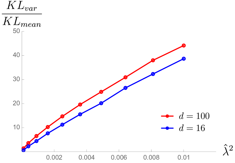
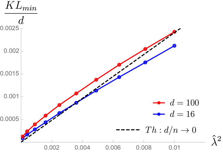
The distance between the generated and the underlying distribution can be also measured in terms of Kullback–Leibler divergence. In Appendix B we provide theoretical analysis when and establish
| (3.5) |
Where the contributions are related to the difference between generated and the underlying distribution in mean and variance. We numerically show in figure 2 (a) that in the regime of interest making the inequality above an approximate equality. Further in fixed, we prove is an increasing function of (see (B.17) for more details). Moreover in Appendix B we show that in this domain the minimum value of scales as . These are confirmed by numerical experiments presented in figure 2 (b).
3.2 Memorization to non-memorization transition
In this subsection, we define and analyze a rigorous metric for memorization to non-memorization transition. For this purpose consider the pairwise distance between probability distributions 777Another possibility is to consider the Wasserstein distance. The simplest version of the Wasserstein distance between the original and generated dataset would require generating samples from the diffusion model and then order computations to find the optimal permutation of the points for computing the distance. This is an extremely computationally expensive technique and we would not pursue it in this paper.
| (3.6) |
We say the model is generalizing well if the generated data distribution is closer to the original dataset compared to the train data, more concretely it is defined by the condition . is a random variable due to randomness in the training data. The diffusion model is considered to be memorizing the training data when the probability that , i.e., is much smaller than unity. Conversely, the model is in the non-memorization regime when . For the linear diffusion model, the pairwise distance between probability distributions is easily calculated to be given by
| (3.7) | ||||
For given we calculate as
| (3.8) |
By performing several simulations over the training set we have plotted the average value of the probability of in Fig. 4.
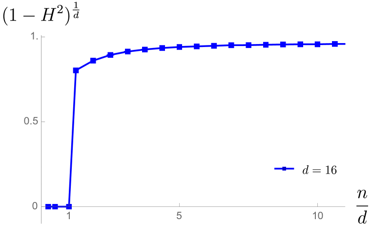
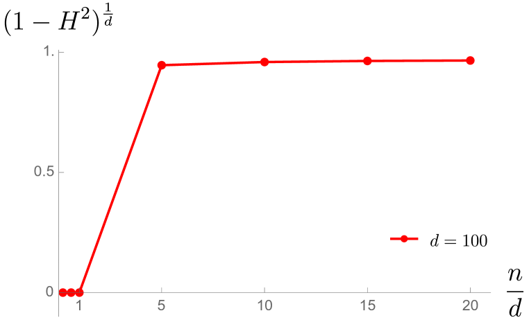
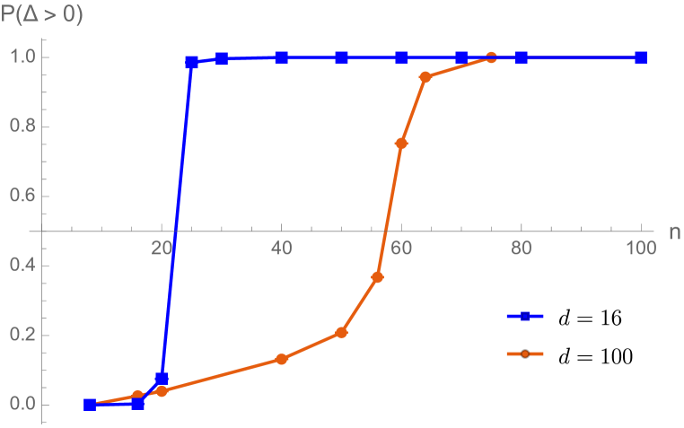
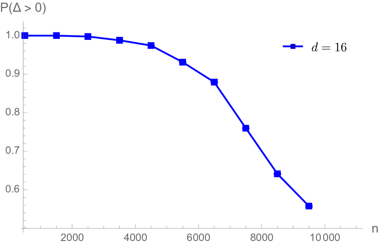
The important regions for are the following:
-
•
: As we increase , probability of increases sharply from zero to one. We call this memorization to non-memorization transition. See Fig. 4 for more details.
-
•
: In this domain saturates near unity at as shown in Fig. 4. From Fig. 3 we see that near , we enter at the regime of convergence where the Hellinger distance between the original and generated distribution decreases relatively faster. This shows the initiation of non-memorization (i.e., ) takes place on the onset of decay of generalization error.
-
•
: In this domain decreases and eventually reaches the value . See Fig. 4 for further details. This is because the distinction between the train and the original dataset disappears in this limit.
4 Non-linear diffusion model
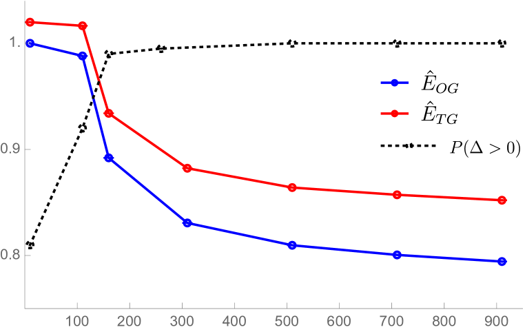
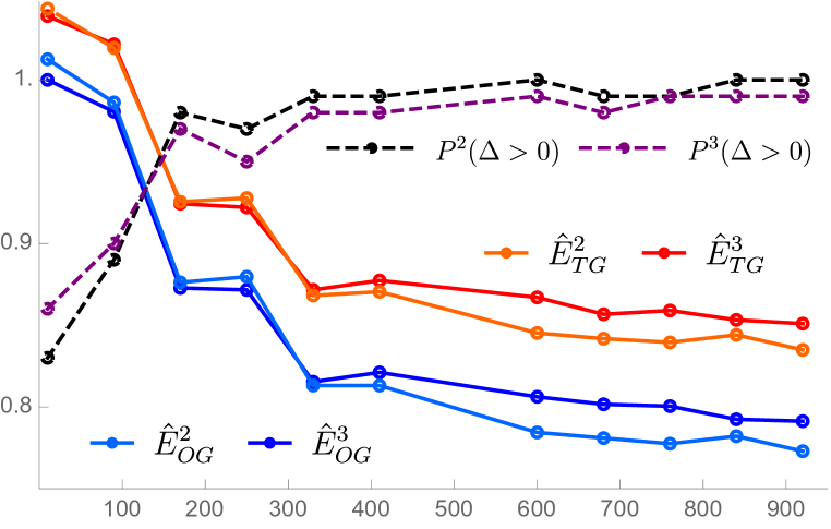
Following the results of the linear diffusion model, we hypothesize that memorization to non-memorization transition happens in the generic diffusion model on the onset of decay in generalization error. In this section, we test our hypothesis on more realistic models. We use the PyTorch-based implementation of the algorithm in [5] as the diffusion model for the experiments in this section.888The computational might be further optimized with the energy-conserving descent method [33]. The denoiser has the structure of U-Net [34] with additional residual connections consisting of positional encoding of the image and attention layers [35, 36, 37]. The generated distribution from the non-linear diffusion model is not necessarily Gaussian, and we face difficulty in evaluating the higher dimensional integration in our measure of distance. For this purpose, we use the following simplified metric, which gives an advantage in terms of computational expense
| (4.1) |
Where we have defined element-wise probability density function Similar definition applies to and . The decay of generalization error and generalization metric for an isotropic Gaussian dataset is plotted in Fig. 5. We see that memorization to non-memorization transition takes places exactly on the onset of a fall phase of the generalization error .
5 Conclusion
In this paper we have defined a mathematically precise metric for memorization to non-memorization transition. We have further constructed a linear diffusion model and analytically established a bound on generalization error that features an interesting scaling law with respect to training dataset size. The model shows the memorization to non-memorization transition, based on the aforementioned metric, aligns with the onset of decay of generalization error. Finally, we have shown that this alignment phenomenon is generic and occurs in realistic non-linear diffusion models.
Furthermore, the proposed metric for memorization to non-memorization transition might be employed to systematically select optimal hyperparameters for model training. Specifically, for a given training set, one can plot the curve of versus across various hyperparameter configurations. The model that transitions to non-memorization at a smaller dataset size may be regarded as the more efficient one (counter-play with the visual quality of the images is also interesting to study). We leave a thorough investigation of these questions to future work.
6 Acknowledgements
I.H. is grateful to Cengiz Pehlevan for mentioning the question, initial collaboration, and several insightful discussions throughout the project. I.H. would like to thank Alexander Atanasov, Hugo Cui, Sab Sainathan, Binxu Wang, and Jacob Zavatone-Veth for useful discussions. The numerical calculations presented in this paper are performed on the clusters of the Kempner Institute for the Study of Natural and Artificial Intelligence at Harvard University and Harvard John A. Paulson School Of Engineering And Applied Sciences. I. H. is supported by U.S. Department of Energy grant DE-SC0009999 and funds from the University of California.
References
- [1] M.R. Douglas, Machine learning as a tool in theoretical science, Nature Reviews Physics 4 (2022) 145.
- [2] M.R. Douglas, Large Language Models, arXiv e-prints (2023) arXiv:2307.05782 [2307.05782].
- [3] J. Sohl-Dickstein, E.A. Weiss, N. Maheswaranathan and S. Ganguli, Deep unsupervised learning using nonequilibrium thermodynamics, 2015.
- [4] Y. Song and S. Ermon, Generative modeling by estimating gradients of the data distribution, Advances in neural information processing systems 32 (2019) .
- [5] J. Ho, A. Jain and P. Abbeel, Denoising diffusion probabilistic models, 2020.
- [6] A. Ramesh, P. Dhariwal, A. Nichol, C. Chu and M. Chen, Hierarchical text-conditional image generation with clip latents, 2022.
- [7] R. Rombach, A. Blattmann, D. Lorenz, P. Esser and B. Ommer, High-resolution image synthesis with latent diffusion models, 2022.
- [8] C. Saharia, W. Chan, S. Saxena, L. Li, J. Whang, E. Denton et al., Photorealistic text-to-image diffusion models with deep language understanding, 2022.
- [9] OpenAI, Sora, 2024, https://openai.com/index/sora/.
- [10] G. Somepalli, V. Singla, M. Goldblum, J. Geiping and T. Goldstein, Diffusion art or digital forgery? investigating data replication in diffusion models, 2022.
- [11] N. Carlini, J. Hayes, M. Nasr, M. Jagielski, V. Sehwag, F. Tramèr et al., Extracting training data from diffusion models, 2023.
- [12] Z. Kadkhodaie, F. Guth, E.P. Simoncelli and S. Mallat, Generalization in diffusion models arises from geometry-adaptive harmonic representation, arXiv preprint arXiv:2310.02557 (2023) .
- [13] I. Halder, A theoretical framework for diffusion-based generative models, 2024, https://github.com/I-Halder/a-theoretical-framework-for-diffusion-based-generative-models/.
- [14] Z. Kadkhodaie and E.P. Simoncelli, Solving linear inverse problems using the prior implicit in a denoiser, in NeurIPS 2020 Workshop on Deep Learning and Inverse Problems, 2020, https://openreview.net/forum?id=RLN7K4U3UST.
- [15] J. Song, C. Meng and S. Ermon, Denoising diffusion implicit models, in International Conference on Learning Representations, 2021, https://openreview.net/forum?id=St1giarCHLP.
- [16] P. Dhariwal and A. Nichol, Diffusion models beat gans on image synthesis, 2021.
- [17] J. Ho and T. Salimans, Classifier-free diffusion guidance, 2022.
- [18] Y. Wu, M. Chen, Z. Li, M. Wang and Y. Wei, Theoretical insights for diffusion guidance: A case study for gaussian mixture models, 2024.
- [19] A. Bradley and P. Nakkiran, Classifier-free guidance is a predictor-corrector, 2024.
- [20] M. Chidambaram, K. Gatmiry, S. Chen, H. Lee and J. Lu, What does guidance do? a fine-grained analysis in a simple setting, 2024.
- [21] T. Yoon, J.Y. Choi, S. Kwon and E.K. Ryu, Diffusion probabilistic models generalize when they fail to memorize, in ICML 2023 Workshop on Structured Probabilistic Inference & Generative Modeling, 2023, https://openreview.net/forum?id=shciCbSk9h.
- [22] K. Shah, S. Chen and A. Klivans, Learning mixtures of gaussians using the ddpm objective, 2023.
- [23] H. Cui, F. Krzakala, E. Vanden-Eijnden and L. Zdeborova, Analysis of learning a flow-based generative model from limited sample complexity, in The Twelfth International Conference on Learning Representations, 2024, https://openreview.net/forum?id=ndCJeysCPe.
- [24] G. Biroli, T. Bonnaire, V. de Bortoli and M. Mézard, Dynamical regimes of diffusion models, 2024.
- [25] P. Wang, H. Zhang, Z. Zhang, S. Chen, Y. Ma and Q. Qu, Diffusion models learn low-dimensional distributions via subspace clustering, 2024.
- [26] A. Hyvärinen, Estimation of non-normalized statistical models by score matching, Journal of Machine Learning Research 6 (2005) 695.
- [27] B. Sriperumbudur, K. Fukumizu, A. Gretton, A. Hyvärinen and R. Kumar, Density estimation in infinite dimensional exponential families, 2017.
- [28] P. Vincent, A connection between score matching and denoising autoencoders, Neural Computation 23 (2011) 1661.
- [29] D. Gross and M. Mezard, The simplest spin glass, Nuclear Physics B 240 (1984) 431.
- [30] M. Rosenblatt, Remarks on Some Nonparametric Estimates of a Density Function, The Annals of Mathematical Statistics 27 (1956) 832 .
- [31] V.A. Epanechnikov, Non-parametric estimation of a multivariate probability density, Theory of Probability & Its Applications 14 (1969) 153 [https://doi.org/10.1137/1114019].
- [32] P.J. Bickel and M. Rosenblatt, On Some Global Measures of the Deviations of Density Function Estimates, The Annals of Statistics 1 (1973) 1071 .
- [33] G.B. De Luca and E. Silverstein, Born-infeld (BI) for AI: Energy-conserving descent (ECD) for optimization, in Proceedings of the 39th International Conference on Machine Learning, K. Chaudhuri, S. Jegelka, L. Song, C. Szepesvari, G. Niu and S. Sabato, eds., vol. 162 of Proceedings of Machine Learning Research, pp. 4918–4936, PMLR, 17–23 Jul, 2022, https://proceedings.mlr.press/v162/de-luca22a.html.
- [34] O. Ronneberger, P. Fischer and T. Brox, U-net: Convolutional networks for biomedical image segmentation, 2015.
- [35] A. Dosovitskiy, L. Beyer, A. Kolesnikov, D. Weissenborn, X. Zhai, T. Unterthiner et al., An image is worth 16x16 words: Transformers for image recognition at scale, in International Conference on Learning Representations, 2021, https://openreview.net/forum?id=YicbFdNTTy.
- [36] Z. Tu, H. Talebi, H. Zhang, F. Yang, P. Milanfar, A. Bovik et al., Maxvit: Multi-axis vision transformer, in European conference on computer vision, pp. 459–479, Springer, 2022.
- [37] W. Peebles and S. Xie, Scalable diffusion models with transformers, in Proceedings of the IEEE/CVF International Conference on Computer Vision, pp. 4195–4205, 2023.
- [38] M.S. Albergo, N.M. Boffi and E. Vanden-Eijnden, Stochastic interpolants: A unifying framework for flows and diffusions, 2023.
- [39] Y. Song, J. Sohl-Dickstein, D.P. Kingma, A. Kumar, S. Ermon and B. Poole, Score-based generative modeling through stochastic differential equations, 2021.
- [40] A. Atanasov, J.A. Zavatone-Veth and C. Pehlevan, Scaling and renormalization in high-dimensional regression, 2024.
- [41] A. Jacot, F. Gabriel and C. Hongler, Neural tangent kernel: Convergence and generalization in neural networks, 2020.
- [42] J. Lee, L. Xiao, S. Schoenholz, Y. Bahri, R. Novak, J. Sohl-Dickstein et al., Wide neural networks of any depth evolve as linear models under gradient descent, Advances in neural information processing systems 32 (2019) .
- [43] J. Lee, L. Xiao, S. Schoenholz, Y. Bahri, R. Novak, J. Sohl-Dickstein et al., Wide neural networks of any depth evolve as linear models under gradient descent, Advances in neural information processing systems 32 (2019) .
- [44] B. Bordelon, A. Canatar and C. Pehlevan, Spectrum dependent learning curves in kernel regression and wide neural networks, 2021.
- [45] A. Canatar, B. Bordelon and C. Pehlevan, Spectral bias and task-model alignment explain generalization in kernel regression and infinitely wide neural networks, Nature Communications 12 (2021) .
- [46] A. Atanasov, B. Bordelon, S. Sainathan and C. Pehlevan, The onset of variance-limited behavior for networks in the lazy and rich regimes, in The Eleventh International Conference on Learning Representations, 2023, https://openreview.net/forum?id=JLINxPOVTh7.
- [47] D.A. Roberts, S. Yaida and B. Hanin, The principles of deep learning theory, vol. 46, Cambridge University Press Cambridge, MA, USA (2022).
- [48] M. Demirtas, J. Halverson, A. Maiti, M.D. Schwartz and K. Stoner, Neural network field theories: non-gaussianity, actions, and locality, Machine Learning: Science and Technology 5 (2024) 015002.
- [49] S. Mei, A. Montanari and P.-M. Nguyen, A mean field view of the landscape of two-layer neural networks, Proceedings of the National Academy of Sciences 115 (2018) .
- [50] G. Yang and E.J. Hu, Tensor programs iv: Feature learning in infinite-width neural networks, in Proceedings of the 38th International Conference on Machine Learning, M. Meila and T. Zhang, eds., vol. 139 of Proceedings of Machine Learning Research, pp. 11727–11737, PMLR, 18–24 Jul, 2021, https://proceedings.mlr.press/v139/yang21c.html.
- [51] B. Bordelon and C. Pehlevan, Self-consistent dynamical field theory of kernel evolution in wide neural networks, Advances in Neural Information Processing Systems 35 (2022) 32240.
- [52] B. Bordelon and C. Pehlevan, Dynamics of finite width kernel and prediction fluctuations in mean field neural networks, Advances in Neural Information Processing Systems 36 (2024) .
Appendix A Connection between ODE and SDE based generative models
In this Appendix we review the connection between stochastic interpolant [38] and stochastic differential equation [39] based generative models. Given two probability density functions , one can construct a stochastic interpolant between and as follows
| (A.1) |
where the function satisfies
| (A.2) | |||||
for some positive constant . Here are drawn independently from a probability measure , and standard normal distribution . The probability distribution of the process satisfies the transport equation999Here we are using the notation .
| (A.3) |
where we defined the velocity101010The expectation is taken independently over and Here is normalized Gaussian distribution of appropriate dimension with vanishing mean and variance.
| (A.4) |
One can estimate the velocity field by minimizing
| (A.5) |
It’s useful to introduce the score function for the probability distribution for making the connection to the stochastic differential equation
| (A.6) |
It can be estimated by minimizing
| (A.7) |
The score function also can be obtained by minimizing the following alternative objective function known as the Fisher divergence
| (A.8) | ||||
To obtain the second line we have ignored the boundary term. Note that for the purpose of minimization the last term is a constant and hence it plays no role hence Fisher divergence can be minimized from a set of samples drawn from easily even if the explicit form of is not known [26]. However, the estimation of is computationally expensive and in practice one uses denoising score matching for estimating the score function [28].
It is easy to put eq. (A.3) into Fokker-Planck-Kolmogorov form
| (A.9) | ||||
For an arbitrary function . From this, we can read off the Itô SDE as follows111111Here represents a standard Wiener process, i.e., is a zero-mean Gaussian stochastic process that satisfies .
| (A.10) | ||||
The first equation is solved forward in time from the initial data and the second one is solved backward in time from the final data . One can recover the probability distribution from the SDE using Feynman–Kac formulae121212A class of exactly solvable models are given by (Ornstein-Uhlenbeck dynamics discussed in the main text is a special case of this equation) (A.11) Where are two positive functions satisfying .
| (A.12) | ||||
Appendix B Generalization error from deterministic equivalence
Consider the scenario when the underlying distribution is Gaussian . The linear denoiser is trained to solve the following linear regression problem
| (B.1) | ||||
The optimal value of the weights that minimizes the standard square loss are given by
| (B.2) |
Here are dimensional matrices whose -th row is respectively (e.g. etc.). Once trained the diffusion model generates data from , .
KL divergence between two PDF is given by
| (B.3) | ||||
We choose to correspond to the underlying distribution and corresponds to the generated distribution. This simplifies the formula above to
| (B.4) |
We define , it follows that
| (B.5) | ||||
Plugging this back in the expression of we get
| (B.6) | ||||
For the difference in mean we get
| (B.7) | ||||
Here we have defined , and special vector such that . It follows that
| (B.8) | ||||
Analytic tractability and various approximations
From (B.6) and (B.7) we see that the generated distribution remains close to the original underlying distribution if both and remain small. To this end, we will find the two following limits useful:
(a) early time approximation is given by with . In this limit and .
(b) late time approximation with . In this limit and . Further taking makes small.
In both these cases we can approximate
| (B.9) |
Plugging this back into the expression of KL divergence (B.4) we get , where
| (B.10) |
First, we focus on
| (B.11) | ||||
We define . We introduce a regulator ridge that we take very small at the end of the calculation. In the limit when keeping fixed we have
| (B.12) | ||||
For the first equality, we used that are independent random variables and the expectation value of vanishes. For the second equality we used that . Next, we used the theory of deterministic equivalence. In particular, we have used , which is valid in the under-parameterized regime (see [40] and references therein for more details on this).
Now we turn to simplify the higher-order terms. We will use the method of deterministic equivalence as shown above without explicitly showing all the steps of regularization.
| (B.13) | ||||
Now we simplify each of the terms one by one. The expression in the first line takes the following form
| (B.14) | ||||
The second line simplifies to
| (B.15) | ||||
The last line takes the following form
| (B.16) | ||||
Putting all the results together we get
| (B.17) | ||||
If we further consider the late time approximation we see that to the leading order due to the last term. Also note that is an increasing function of .
Our analytical calculation in this appendix can be easily generalized to the region of smaller values of train dataset size compared to the dimension of the data distribution, perhaps with the addition of a ridge parameter. Other possibilities include studying a (stack of) wide neural network in the kernel approximation regime [41, 42, 43, 44, 45, 46, 47, 48] or in mean field regime [49, 50, 51, 52] instead of a linear diffusion model.