Integrating Dual Prototypes for Task-Wise Adaption in Pre-Trained Model-Based Class-Incremental Learning

Abstract

Class-incremental learning (CIL) aims to acquire new classes while conserving historical knowledge incrementally. Despite existing pre-trained model (PTM) based methods performing excellently in CIL, it is better to fine-tune them on downstream incremental tasks with massive patterns unknown to PTMs. However, using task streams for fine-tuning could lead to catastrophic forgetting that will erase the knowledge in PTMs. This paper proposes the Dual Prototype network for Task-wise Adaption (DPTA) of PTM-based CIL. For each incremental learning task, a task-wise adapter module is built to fine-tune the PTM, where the center-adapt loss forces the representation to be more centrally clustered and class separable. The dual prototype network improves the prediction process by enabling test-time adapter selection, where the raw prototypes deduce several possible task indexes of test samples to select suitable adapter modules for PTM, and the augmented prototypes that could separate highly correlated classes are utilized to determine the final result. Experiments on several benchmark datasets demonstrate the state-of-the-art performance of DPTA. The code will be open-sourced after the paper is published.

1 Introduction

With the rapid developments of deep learning, deep models have achieved remarkable performances in many scenarios [4, 5, 23, 15, 53, 54]. These models generally use independently and identically distributed (i.i.d.) samples for training. However, in the real world, data could come in stream form [11] with various distributions. If deep learning models are trained with non-i.i.d data streams, their previously acquired knowledge could be erased by the data with new distributions, known as the catastrophic forgetting [10]. Therefore, there is an urgent need for a stable and incremental learner in real-world applications.

Among many types [7] of incremental learning (also known as continual learning), class-incremental learning (CIL) receives the most attention [64] as it is more relevant to real-world scenarios [43]. CIL builds a model to continually learn new classes from data streams. Previous representative works for CIL were generally based on sample replay, [32, 25], regularization [28] and distillation [33]. These methods require additional replay samples and more trainable parameters to perform excellently. Recently, Pre-Trained Model (PTM)-based methods [62] have achieved milestone gains in CIL since they utilize a robust PTM with strong generalizability pre-trained on large-scale corpus [31] or image datasets [2, 8]. These algorithms freeze the weights of PTM during CIL training, so that the knowledge acquired from previous pre-training is preserved, thus effectively avoiding catastrophic forgetting.

Despite surpassing previous approaches, massive patterns in downstream incremental tasks are unexposed to PTMs during pre-training. Most existing PTM-based methods calculate the similarities [3] between test samples and class prototypes built from PTM-extracted sample representations for classification. If the PTM is not adequately adapted to downstream tasks, some prototypes could be highly correlated [29], resulting in a close similarity between test samples and these prototypes. Worse still, the number of highly correlated prototypes could continually rise in the CIL process and significantly reduce the classification performance. However, as tasks arrive as streams in CIL, it is impractical to leverage all training samples for fine-tuning. Meanwhile, utilizing task streams to train the PTM sequentially could cause catastrophic forgetting again.

Recently, some approaches [61, 37, 63] suggest the task adaption strategy for PTM-based methods, which assigns several free-loading and lightweight fine-tuning modules for incremental tasks, such as prompt [47], scale & shift [22], adapter [14], or Visual Prompt Tuning (VPT) [16], then load the appropriate module trained in the corresponding task for PTM to extract representations. However, as task indexes are only known in the training phase of CIL, these modules cannot be wisely selected. Previous methods must design a complex process for query matching [47], combination [37] or ensemble [63].

To tackle the above issues, we present the Dual Prototype network for Task-wise Adaption (DPTA) of PTM-based CIL in this paper. Similar to other task adaption methods, an adapter is created for PTM’s adaption on each downstream task. We notice that the top-K prediction with prototypes could maintain a high accuracy during the CIL process, which can be considered reliable information for selecting suitable adapters. Accordingly, we propose the Dual Prototype Network, which uses a two-step prediction method, decomposing the problem into a high-accuracy top-K prediction sub-problem and a $K$-class classification sub-problem. Specifically, a set of raw prototypes is built with the original PTM to predict the sample’s top-K possible labels, from which the sample’s related task indexes can be deduced, so adapters can be task-wise selected accordingly. The set of augmented prototypes is built with task-adapted PTM and utilized together with task-wise adapters to predict the label of test samples. Meanwhile, to avoid the arising of highly correlated augmented prototypes, we use a center-adapt loss for fine-tuning to make extracted representations gathered toward class centers while increasing inter-class distances in feature space. The main contributions of our work are summarized as follows:

• We improve the task-wise adaption of PTM-based CIL by introducing top-K degradation, degrade the classification problem into a $K$-class classification sub-problem and accurately select related task-wise adapters.

• We propose the Dual Prototype Network (DPN), where the raw prototypes predict each sample’s top-K class labels and augmented prototypes predict the top-1 class label. We also improve the training of task-wise adapters with the center-adapt loss, making the augmented prototypes more class-distinctive and centrally clustered.

• Extensive experiments on multiple incremental datasets with advanced methods show that our method can achieve state-of-the-art performance. In addition, we analyze how to enhance the accuracy of DPTA.

2 Related works

2.1 Class-Incremental Learning and Previous Methods

In CIL, the model will durably absorb new class knowledge from training task streams in the training phase and correctly predict the samples without their task indexes in the test phase. Previous CIL methods can be generally divided into the following types: Replay-based methods [33, 26, 6, 24] deposit typical samples into a buffer, which is called in subsequent training to recover old class knowledge. Regularization-based methods [28, 1, 56] protect the knowledge obtained on the old task by adding regularization to limit the model parameters updating on the new task. Distillation-based methods [32, 36, 39, 58] retain the knowledge of the previous task through knowledge distillation between the old and new model. Parameter isolation methods [25, 34, 49] set different parameters for the model with each task to prevent forgetting. These methods typically require longer training of a large neural network, and some must store representative samples for replay, which presents challenges in training time and memory space.

2.2 Class-Incremental Learning with Pre-Trained Models

With the strong generalization ability of pre-trained models, they have been introduced to CIL for robust representation extraction. SimpleCIL [61] demonstrates that excellent CIL classification accuracy can be achieved by only building prototypes with raw PTMs. RanPAC [27] reveals that using the random projection for PTM outputs could form a more separative representation space. The initial idea to adapt the PTM to downstream tasks is first-task adaption in ADAM [61], which only fine-tunes the model on the first task to obtain enhanced performance than using the original PTM. But the gain is sometimes limited especially when samples from different tasks are poorly correlated. A series of prompt-based works [47, 44, 46, 37] have emerged by establishing a prompt pool to accommodate numerous prompts trained on task streams, where selecting the appropriate prompt for test samples poses a significant challenge in such methods. L2P [47] designs a key-query matching strategy to obtain fit prompts, DualPrompt [46] adds prompts to different layers and decouples them into expert and common groups. CODA-Prompt [37] introduces the attention mechanism on prompt building and creates a weighted combination of prompts. In addition, EASE [63] proved experimentally that the prototype of one class can be calculated by linearly integrating the remaining classes’ prototypes, thereby suggesting a subspace expansion and ensemble process with all task-adapted modules.

3 Preliminaries

In this section, we propose a brief introduction to PTM-based class-incremental learning and the strengths and weaknesses of prototype classification.

3.1 Class-Incremental Learning with PTMs

In the CIL scenario, a learning system will continually learn from streaming training data, which consists of many new classes in each incremental learning task. The system is required to make correct predictions without extra information, like the task index of test samples [43]. Assume that there are $T$ tasks, their training sets are denoted as $D_{1},D_{2},\cdots,D_{t}$, where $D_{t}=\{(\boldsymbol{x_{i}},y_{i})\}_{i=1}^{n_{t}}$ is the $t$-th training set that has $n_{t}$ samples and $D_{1},D_{2},\cdots,D_{t}$ are non-i.i.d. In the $t$-th task, only $D_{t}$ can be accessed for training. The learning system is trained to obtain an optimal model $f^{*}(\boldsymbol{x}):\mathcal{X}\xrightarrow{}\mathcal{Y}$ that minimizes the expected risk for all classes in $D_{1}\cup\cdots\cup D_{t}$.

$$f^{*}(\boldsymbol{x})=\underset{f\in\mathcal{H}}{\arg\min}\mathop{\mathbb{E}}\nolimits_{(\boldsymbol{x},y)\in D_{1}\cup\cdots\cup D_{t}}[\mathbb{I}(f(\boldsymbol{x})\neq y)].$$ (1)

where $\mathbb{I}$ is the indicator function and $\mathcal{H}$ denotes the hypothesis space of model $f$.

An advanced and effective methodology [62] for CIL is to utilize pre-trained models (e.g. Vision Transformer [9] in image classification) to extract the representation of samples. The decision model of PTM-based methods can be expressed as $f(\boldsymbol{x})=W^{\mathrm{T}}\phi(\boldsymbol{x})$, where the $\phi(\cdot):\mathbb{R}^{d}\xrightarrow{}\mathbb{R}^{h}$ is the PTM feature extractor, and $W$ is a customized classifier to separate representations extracted by PTM. Since the PTM acquires rich relevant knowledge from the pre-training, the extracted representation has both generalizability and adaptivity [61]. Meanwhile, weights of the PTM feature extractor are frozen during incremental learning, which also effectively prevents catastrophic forgetting.

3.2 Nearest Class Mean Classifier in CIL

The fully connected layer with softmax activation function is [19] is commonly used for classification in deep networks, but the continuously increasing number of classes in CIL makes it ineffective. A widely used classifier in CIL is the prototype-based Nearest Class Mean (NCM) [50]. Upon the arrival of one class training data, the representations are extracted by an encoder model like PTM, and the prototype for this class is calculated as the mean value of representations. Suppose there are $M_{k}$ training samples in class $k$, $y_{i}$ is the label of sample $\boldsymbol{x_{i}}$. The prototype for class $k$ is denoted as $\boldsymbol{p_{k}}$, which can be calculated in the following form:

$$\boldsymbol{p_{k}}=\frac{1}{M_{k}}\sum_{j=1}^{M_{k}}\mathbb{I}(y_{i}=k)\phi(\boldsymbol{x_{i}}).$$ (2)

In the test phase, the similarity between samples and each existing prototype is computed. The commonly used similarity measure is cosine similarity [52], denoted as $Sim(\boldsymbol{x},\boldsymbol{y})_{\cos}$ in this paper.

Assuming that there are $N$ classes in $D_{1},D_{2},\cdots,D_{t}$, the prediction $\hat{y}_{i}$ of the test sample $x_{i}$ can be written as:

$$\hat{y}_{i}=\underset{k=1,2,...N}{\arg\max}(Sim(\phi(\boldsymbol{x_{i}}),\boldsymbol{p_{k}})_{\cos}).$$ (3)

Since the mean value greatly compresses the information and only reflects limited class features, there might be some highly correlated prototypes in the feature space [27], which have a close distance and a higher correlation coefficient. The class separability of these prototypes is generally poor because the test sample’s similarities to these prototypes are very close. Even if catastrophic forgetting is mitigated by PTM, the number of similar prototypes will rise gradually, markedly decreasing the classification accuracy.

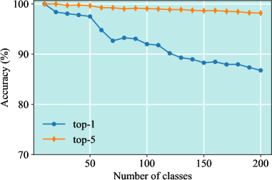
Figure 1: The accuracy of NCM top-1 and top-5 predictions in the CUB-200 datasets, where the accuracy of the top-5 group ranged from 98% to 100%. The prototypes were built with a pre-trained VIT-B/16-IN21K without fine-tuning.

Although the NCM has the above limitations, we found that the top-K possible labels of the test sample, i.e., the K nearest prototypes to the test sample representation, can be more accurately predicted by prototypes constructed from the original PTM. Figure 1 shows that top-5 accuracy decreases much slower than top-1, which indicates that the number of highly correlated prototypes is limited. Therefore, we can select top-K labels of the sample that are hard to distinguish and then use more effective strategies for this new $K$-class classification problem. We refer to this concept as top-K degradation for CIL. The original classification problem is decomposed into a smaller sub-problem through top-K degradation. Moreover, top-K labels also serve as the evidence for selecting task adapters at test time, we will discuss this in the next section.

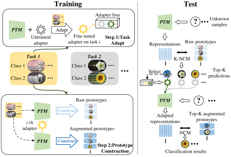
Figure 2: Illustration of DPTA. Left: Training. When a new task $i$ arrives, we fine-tune and save the $i$-$th$ task-wise adapter, then use the raw PTM and adapted PTM to construct two prototypes of all classes in the $i$-$th$ task. Right: Test. The top-K label of the sample is predicted using the raw prototypes to select several tuned adapters. Then use augmented prototypes to predict the exact label of the sample.

4 Methodology

As discussed above, relying on freezing PTMs and prototypes cannot effectively separate some classes in downstream tasks, but fine-tuning PTMs incrementally will lead to catastrophic forgetting. Therefore, as shown in Figure 2, we assign an adapter module to each task and try to make the augmented prototypes extracted by the adapted PTM conducive to prototype classification. In the testing phase, we adopt a two-step inference method: first, the underlying task index of the test sample is deduced from the known information; then, appropriate task-wise adapters are loaded and the classification result is calculated from augmented prototypes.

In the following subsections, we first introduce task-wise adaption and center-adapt loss, by which we improve the separability of the fine-tuned PTM representation designed for prototypes; then provide the dual prototype network, the classifier for DPTA; finally, we describe the test process of the proposed DPTA at the end of this section.

4.1 Task-wise Adaption with Center-Adapt Loss

We select the adapter [14] as the PTM fine-tuning module as it has excellent performance with fewer trainable parameters. An adapter adds a lightweight bottleneck module in each Transformer encoder block, where each bottleneck module consists of a down-projection layer $W_{dp}\in\mathbb{R}^{h\times r}$, an up-projection layer $W_{up}\in\mathbb{R}^{r\times h}$, and a nonlinear activation function (set to the ReLU [20]). Adapter units map inputs by adding the residual term as:

$$\boldsymbol{z^{\prime}_{i}}=\boldsymbol{z_{i}}+ReLU(\boldsymbol{z_{i}}W_{dp})W_{up},$$ (4)

where $\boldsymbol{z_{i}}$ and $\boldsymbol{z^{\prime}_{i}}$ are feature vectors of input and output respectively.

The underlying reason for highly correlated prototypes is that the original PTM could extract poorly discriminated representations of some classes in downstream tasks without adaption (Figure 3). To enhance the effect of task adaption, we propose the center-adapt loss to fine-tune the PTM with adapters. Since prototypes are the centers of sample representations of their respective classes, if the sample representations of each class are spatially clustered like a hypersphere and gathered towards its center, more accurate results can be obtained using the prototype. Specifically, it can be achieved by utilizing the Center Loss (CL) [48] to train the model, denoted as the following forms:

$$\mathcal{L}_{C}=\frac{1}{2}\sum_{i=1}^{M}||\boldsymbol{x_{i}}-\boldsymbol{c_{y_{i}}}||^{2}_{2},$$ (5)

where the $\boldsymbol{c_{y_{i}}}$ is the center of sample representations in class $i$. CL minimizes the distance of each sample in the mini-batch from the center of the corresponding classes, where all the centers $\boldsymbol{c_{y_{i}}}$ are dynamically updated with training. Still, the main goal of fine-tuning is to improve the class separability of the PTM representation, so the center-adapt loss is a weighted combination of cross-entropy (CE) loss [59] and CL, which can be written in the following form:

$$\mathcal{L}_{CA}=\mathcal{L}_{CE}+\lambda\mathcal{L}_{C},$$ (6)

where $\lambda$ is a constant weighting factor for the CL.

When the training set $D_{i}$ of task $i$ arrives, we create a temporary linear output layer for computing the CE loss and remove it when the next task arrives. The task adaption is performed on the $D_{i}$, i.e. updating the specific adapter’s parameters with the frozen PTM and linear layer by center-adapt loss. After the task adaption, the parameters of adapter $i$ are frozen.

Fine-tuning the PTM using lightweight modules can be viewed as projecting the extracted representation into a feature subspace. With the center-adapt loss, the sample representations in subspace (Figure 3) are more conducive to prototype classification since they will be clustered towards the center with a lower intra-class distance by CL and have a higher inter-class distance by CE loss. Moreover, as those off-task samples (light blue ‘x’ markers in Figure 3) are not involved in the particular task adaption process, their representations in the subspace will lie significantly farther from all class centers compared with on-task samples belonging to their respective classes. For example, if there are $m$ classes on task $t_{n}$, $\forall\boldsymbol{x_{i}}\notin$ $t_{n}$ and $\forall\boldsymbol{x_{j}}\in$ class $k=1,2...,m$ in task $t_{n}$, as the spatial distance and cosine similarity have a strong negative correlation, then it generally has:

$$Sim(\phi^{A_{t_{n}}}(\boldsymbol{x_{i}}),\boldsymbol{p^{aug}_{k}})_{\cos}<Sim(\phi^{A_{t_{n}}}(\boldsymbol{x_{j}}),\boldsymbol{p^{aug}_{k}})_{\cos},$$ (7)

where the $\phi^{A_{t_{n}}}$ is the PTM loaded with the adapter corresponding to task $t_{n}$, and $\boldsymbol{p^{aug}_{k}}$ is the augmented prototype of class $k$ constructed with the adapted PTM.

Meanwhile, if sample $\boldsymbol{x_{j}}$ uses the PTM with wrong adapters $t\neq t_{n}$ for feature extraction (gray ‘v’ markers in Figure 3), it will be projected into another subspace far away from on-task class centers. Similarly, it has:

$$Sim(\phi^{A_{t}\neq A_{t_{n}}}(\boldsymbol{x_{j}}),\boldsymbol{p^{aug}_{k}})_{\cos}<Sim(\phi^{A_{t_{n}}}(\boldsymbol{x_{j}}),\boldsymbol{p^{aug}_{k}})_{\cos},$$ (8)

The two cases $\phi^{A_{t_{n}}}(\boldsymbol{x_{i}})$ and $\phi^{A_{t}\neq A_{t_{n}}}(\boldsymbol{x_{j}})$ are considered as outliers for $\boldsymbol{p^{aug}_{k}}$ in subspace $t_{n}$, which suggests that augmented prototypes could separate sample representations from the PTM that loads the wrong adapter.

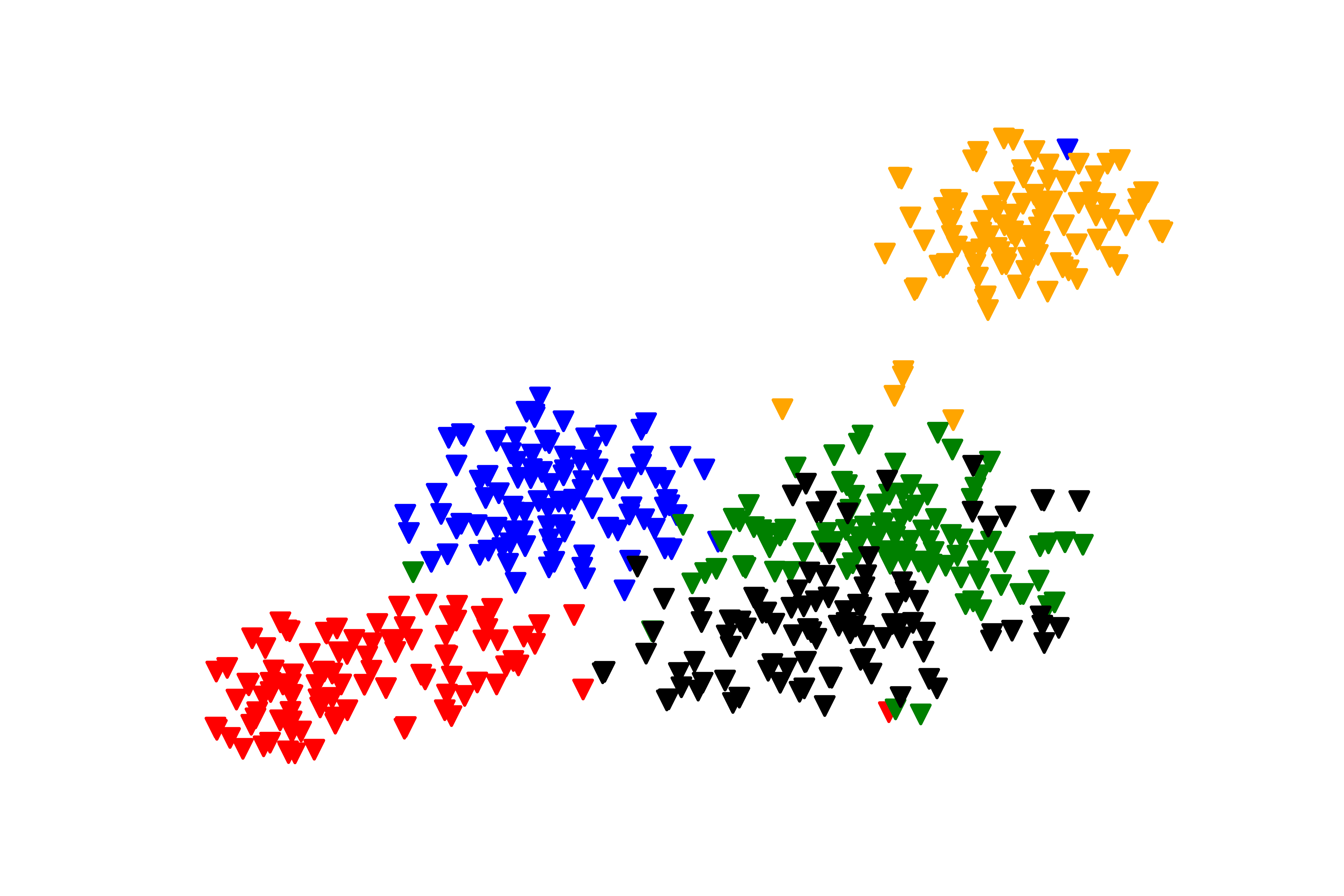
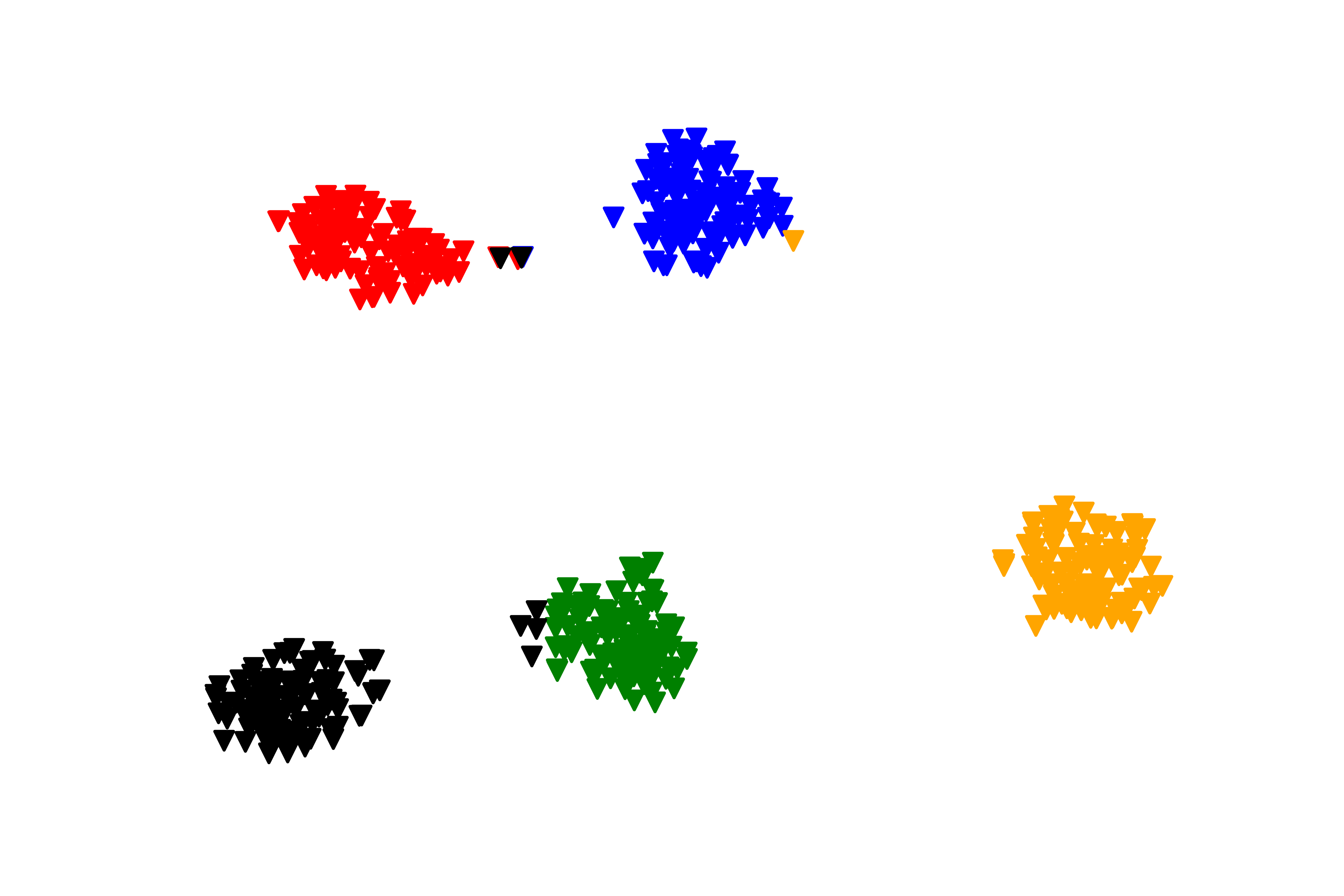
[On-task samples w/o adaption] [All samples w/o adaption]
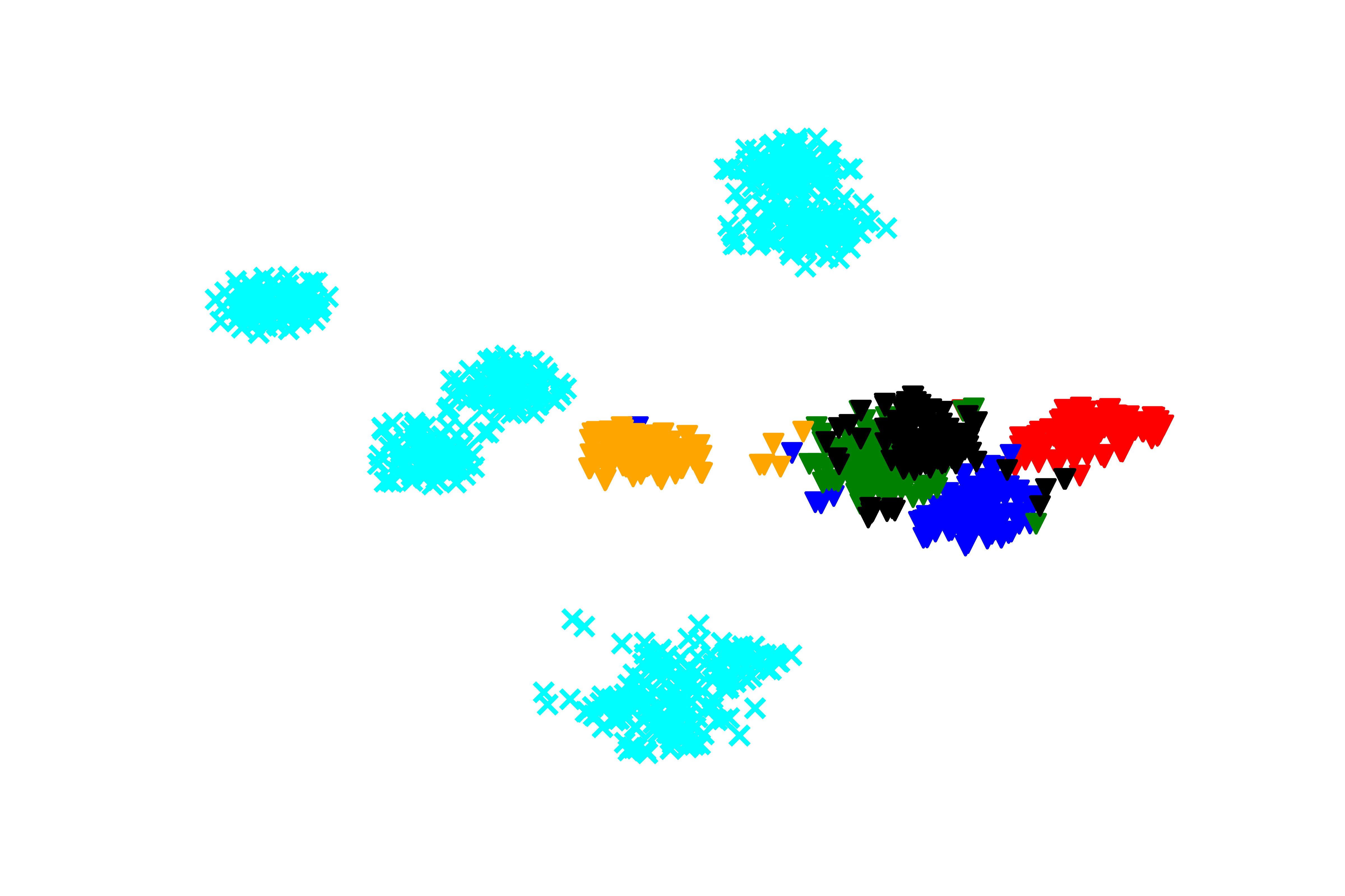
[On-task samples in subspace] [All samples in subspace]

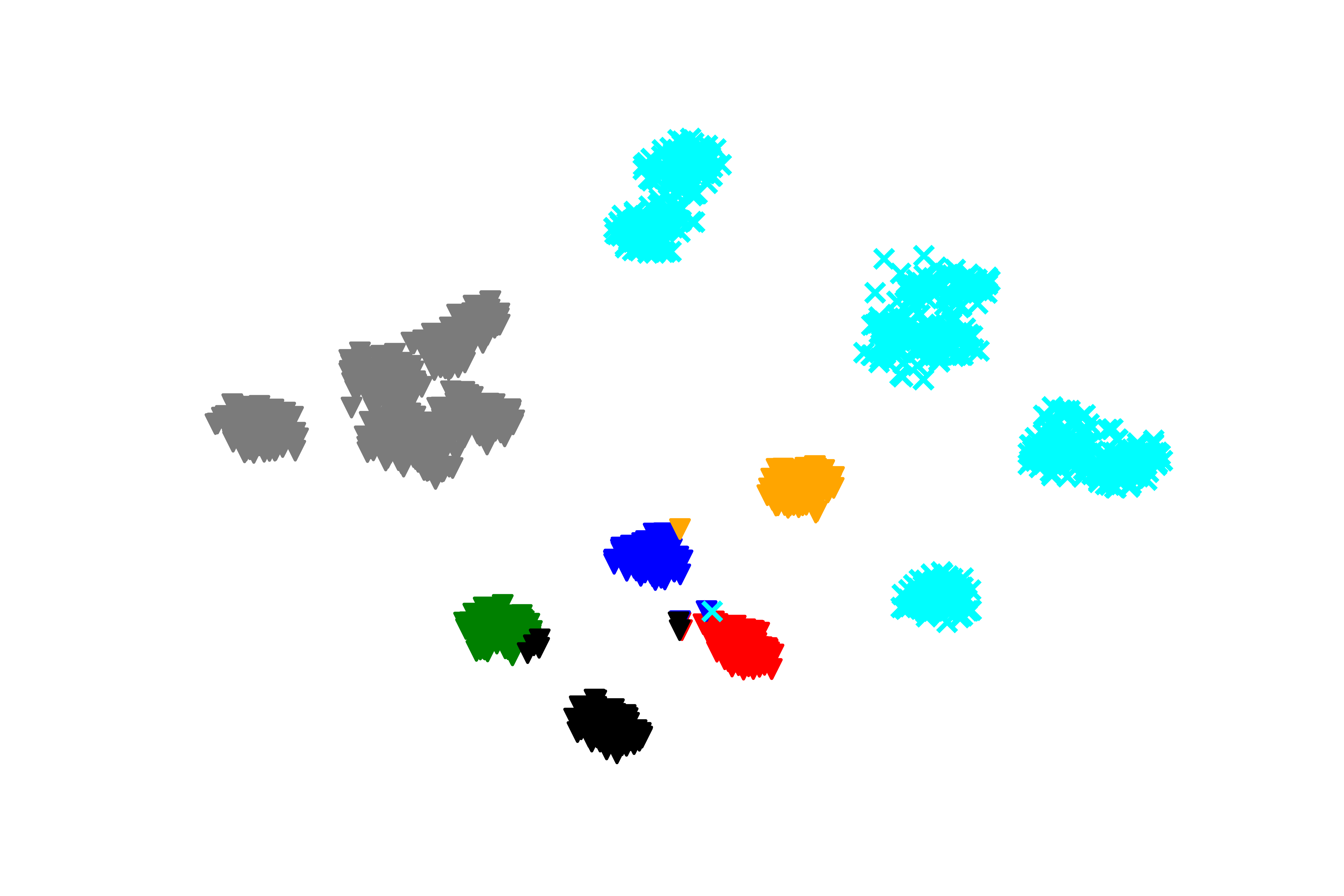
Figure 3: t-SNE [40] visualizations of original feature space and task-adapted subspace $t_{n}$ trained with center-adapt loss, where samples come from a subset of the VTAB dataset.

4.2 Dual Prototype Network

Based on top-K degradation, we propose the Dual Prototype Network (DPN) that has two prototypes for each class in the dataset to replace the previous single prototype set.

The first prototype set is named raw prototypes as built through Eq.(2) without task-wise adaption, which is used to predict top-K possible labels for test samples and obtain extra salutary information from top-K labels. For example, up to $K$ possible task indexes of the sample can be obtained if the correspondence between labels and task indexes is preserved in the training phase.

The second prototype set named augmented prototypes predicts the top-1 label with extra information from the top-K predictions. We build augmented prototypes using the mean value of representation extracted by the adapted PTM, denoted in the following form:

$$\boldsymbol{p^{aug}_{k}}=\frac{1}{M_{k}}\sum_{j=1}^{M}\mathbb{I}(y_{j}=k)\phi^{A_{t_{k}}}(\boldsymbol{x_{j}}).$$ (9)

After the task adaption training with $D_{i}$, the raw prototypes and augmented prototypes of the classes are computed using Eq.(2) and Eq.(9) respectively. After completing the training of $n$ tasks, we obtain $n$ adapters, $\sum_{i=1}^{n}N_{i}$ raw prototypes and augmented prototypes respectively, where $N_{i}$ denotes the number of classes in $i$-th task.

4.3 Prediction process of DPTA

DPTA is a combination of DPN and task-wise adapters. The prediction process of DPTA can be divided into two steps. Suppose $(\boldsymbol{x_{i}},y_{i})$ are the feature and the label of a sample, $f(\boldsymbol{x_{i}}):\mathcal{X}\xrightarrow{}\mathcal{Y}$ denotes the prediction of DPN. First, raw prototypes are utilized to predict the top-K class labels as follows:

$$Y^{topK}_{i}=\underset{k=1,2,...N}{K\text{-}\arg\max}(Sim(\phi(\boldsymbol{x_{i}}),\boldsymbol{p^{raw}_{k}})_{\cos}),$$ (10)

then the corresponding task IDs are obtained based on the top-K labels. If the preset $K$ exceeds the number of raw prototypes $n$, it can be temporarily set to $n$ until sufficient raw prototypes are attained.

With the accurate top-K labels and corresponding task IDs from raw prototypes, it is only necessary to select the adapters with given task IDs to PTM and calculate the cosine similarities between the test sample’s adapted representations and augmented prototypes corresponding to the top-K classes, rather than comparing with all augmented prototypes, thereby greatly reducing the computation time without losing accuracy. Several selected adapters are loaded for the PTM according to the task IDs to output representations of the test sample. The cosine similarity is calculated between task-adapted representations and top-K augmented prototypes, and the index of the nearest augmented prototype is the predicted label $\hat{y}_{i}$ for the test sample $\boldsymbol{x_{i}}$. It can be denoted as the following form:

$$\hat{y}_{i}=\underset{k\in Y^{topK}_{i}}{\arg\max}(Sim(\phi^{A_{t(k)}}(\boldsymbol{x_{i}}),\boldsymbol{p^{aug}_{k}})_{\cos}),$$ (11)

where the $t(k)$ denotes the task ID of the class $k$.

Assuming that the sample $\boldsymbol{x_{i}}$ comes from task $t_{i}$. From the conclusion in Eq.(7),(8), $\phi^{A_{t(k)}}(\boldsymbol{x_{i}})$ extracted by all $\phi^{A_{t(k)}}\neq\phi^{A_{t_{i}}}$ will be considered as outliers with a lower similarity, thus all the class $k$ that $t(k)\neq t_{i}$ are eliminated generally. Meanwhile, the classes on task $t_{i}$ are easier to separate after the task adaption. Therefore, indistinguishable classes from highly correlated raw prototypes are more likely to be correctly classified by augmented prototypes.

Making correct predictions by the DPN requires that both prototype sets give accurate results, since their inference are based on similarity maximization, their predictions are generally not independent. Therefore, from the conditional probability formula [35], the expected performance boundary of DPN can be written in the following form:

$$\underset{\boldsymbol{x_{i}}\in\mathcal{X},y_{i}\in\mathcal{Y}}{\mathbb{E}}[\mathbb{I}(y_{i}=f(\boldsymbol{x_{i}}))]= \mathbb{E}[\mathbb{I}(y_{i}=\hat{y}_{i})|\mathbb{I}(y_{i}\in Y^{topK}_{i})]$$

$$*\mathbb{E}[\mathbb{I}(y_{i}\in Y^{topK}_{i})].$$ (12)

Eq.(4.3) indicates that the DPN’s performance can be improved by enhancing the prediction accuracy of two prototypes separately. According to Figure 1, the Top-K label set can be precisely obtained by PTMs without fine-tuning. Therefore, the augmented prototype set is the core of DPN. It must contain far richer information than raw prototypes, otherwise it will degenerate into one prototype set case. When all predictions from augmented prototypes are correct, the DPN will reach the upper bound of expected performance, i.e., the top-K prediction accuracy.

Table 1: Average accuracy $\overline{A}$ and final accuracy $A_{F}$ results on six benchmark datasets, where the best results achieved on all benchmarks are in bold. All methods used here are exemplar-free methods in which no replay samples are required.

Methods	CIFAR		CARS		CUB		ImageNet-A		ImageNet-R		VTAB
	$\overline{A}$	$A_{F}$	$\overline{A}$	$A_{F}$	$\overline{A}$	$A_{F}$	$\overline{A}$	$A_{F}$	$\overline{A}$	$A_{F}$	$\overline{A}$	$A_{F}$
Finetune	63.51	52.10	42.12	40.64	67.84	54.59	46.42	42.20	48.56	47.28	50.72	49.65
LWF	46.39	41.02	56.33	46.94	49.93	34.02	38.75	26.94	42.99	36.64	40.49	27.63
SDC	68.45	64.02	61.58	52.12	71.63	67.36	29.23	27.72	53.18	50.05	48.03	26.21
ESN	87.15	80.37	46.32	42.25	65.70	63.11	44.56	31.44	62.53	57.23	81.54	62.12
L2P	85.95	79.96	47.95	43.21	67.07	56.26	47.12	38.49	69.51	64.34	77.10	77.05
DualPrompt	87.89	81.17	52.72	47.62	77.43	66.58	53.75	41.64	67.45	62.31	83.23	81.20
CODA-Prompt	89.15	81.94	55.95	48.27	84.02	73.38	53.56	42.92	68.52	63.25	83.95	83.01
SimpleCIL	87.57	81.26	65.54	54.78	92.15	86.72	59.77	48.91	62.55	54.52	86.01	84.43
ADAM(Adapter)	90.55	85.10	66.76	56.25	92.16	86.73	60.49	49.75	72.32	64.37	86.04	84.46
ADAM(VPT-S)	90.52	85.21	66.76	56.25	91.99	86.50	59.43	47.62	71.93	63.52	87.25	85.37
EASE	92.45	87.05	76.45	64.22	92.23	86.80	65.35	55.04	81.73	76.17	93.62	93.54
DPTA(ours)	92.70	88.51	79.46	68.28	92.56	87.23	68.77	58.08	84.79	78.29	94.44	93.73

5 Experiments

In this section, we conduct extensive experiments on six benchmark datasets, including a comparison with state-of-the-art methods in 5.2 and an ablation study to prove the effectiveness of DPTA in 5.3. In addition, we analyzed why the core of DPTA are augmented prototypes in 5.4. Extra experiments are proposed in the supplementary.

5.1 Implementation Details

Dataset and split. The commonly used PTM in most CIL methods is ViT-B/16-IN21K [9]. Considering it was pre-trained on the ImageNet 21K dataset, we chose six datasets that have large domain gaps with ImageNet for CIL benchmarks, including CIFAR-100 [18], CUB-200 [41], ImageNet-A-200 [13], ImageNet-R-200 [12], CARS-196 [17] and VTAB-50 [57], where the number following the dataset is the total number of classes included. Following the ‘B/Base-m, Inc-n’ rule proposed by Zhou et al. [61], We slice each of the above six datasets into CIFAR B0 Inc10, CUB B0 Inc10, ImageNet-A B0 Inc20, ImageNet-R B0 Inc 20, Cars B16 Inc 20 and VTAB B0 Inc10 for experiment similar to [63], where $m$ is the number of classes in the first incremental task, and $n$ represents that of every remain stage. $m=0$ indicates classes in the dataset are equally divided to each task. For a fair comparison, we ensure that the training and test datasets are identical for all methods.
Comparison with state-of-the-art. Several baselines or state-of-the-art (SOTA) methods are selected for comparison in this paper, including LWF [21], SDC [55], ESN [45], L2P [47], Dual-Prompt [46], CODA-Prompt [37], SimpleCIL [61], ADAM [61], and EASE[63]. We also report the result that finetunes the PTM sequentially (Finetune). All methods that include PTM use ViT-B/16-IN21K to ensure fairness.
Programming and parameters. We run experiments on NVIDIA A4000 with PyTorch 2.4.1 [30]. DPTA is programmed based on the Pilot [38], an easy-to-use toolbox for PTM-based CIL. The parameter settings of the other methods were taken from the recommended values in the corresponding papers or Pilot. The settings of some subordinate parameters in DPTA like learning rate, optimizer, and batch size are manually set in each experiment, where the learning rate uses cosine annealing. For DPTA’s specific parameters, the $K$ value takes five in all benchmarks. The loss function’s combined weight $\lambda$ is generally set to 0.0001 and will be higher on some datasets. For all methods, referring to the Pilot’s setup [38], we fix the random seed to 1993 in the training and testing phases to ensure fairness and reproducible results. The details of the experimental settings can be found in the supplementary material.
Evaluation metrics. Following the benchmark protocol setting proposed by Rebuffi et al. [32], we use $A_{b}$ to denote the $b$-stage accuracy on the test set that includes all known classes after trained with $D_{1},D_{2},\cdots,D_{b}$, $\overline{A}=\frac{1}{T}\sum_{b=1}^{T}A_{b}$ is average stage accuracy over $T$ tasks, and $A_{F}$ is the final accuracy on the test set that includes all classes. We use two metrics $\overline{A}$ and $A_{F}$ to evaluate the model performance, which reflects the model’s dynamic learning capacity and final generalization ability respectively.

5.2 Benchmark Comparison

This subsection compares the proposed DPTA with SOTA or baseline methods on the six datasets above, where the results are reported in Table 1. DPTA achieves the highest classification accuracy on all six datasets, outperforming all the previous SOTA or baseline methods significantly. Comparison with ADAM, L2P, Dualprompt, and CODA-prompt demonstrates the effectiveness of DPTA’s task-wise adaptation over the first-task adaption and prompt-based matching or combination. Meanwhile, DPTA exceeds the most recent method EASE by up to 4%, which demonstrates that selecting proper adapters could achieve better results than linearly integrating them.

Moreover, we compare the DPTA with several milestone baseline methods that require replay samples (Exemplars), including the iCaRL [32], DER [51], FOSTER [42], and MEMO [60]. These methods are implemented with the same ViT-B/16-IN21K PTM as DPTA, where exemplars are taken as 20 samples per class, as shown in Table 2. The results indicate that DPTA could still have a competitive performance without exemplars and reach the optimal accuracy in these methods.

Table 2: Comparison to SOTA replay-based methods. Those methods are trained with the same ViT-B/16-IN21K PTM.

Methods	CIFAR		ImageNet-A		ImageNet-R
	$\overline{A}$	$A_{F}$	$\overline{A}$	$A_{F}$	$\overline{A}$	$A_{F}$
iCaRL	82.36	73.67	29.13	16.15	72.35	60.54
DER	86.11	77.52	33.72	22.13	80.36	74.26
FOSTER	89.76	84.54	34.55	23.34	81.24	74.43
MEMO	84.33	75.56	36.54	24.43	74.12	66.45
DPTA(ours)	92.70	88.51	68.77	58.08	84.79	78.29

In addition, we investigate the trainable parameters of different methods. The proportion of trainable parameters to model parameters and the $A_{F}$ accuracy on ImageNet-R B80 Inc40 are reported in Figure 4. It is illustrated that the number of trainable parameters in DPTA equals the SOTA method EASE and requires the approximal scale (0.1%-1%) as these prompt-based methods.

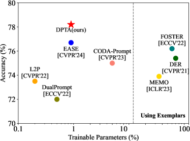
Figure 4: Trainable parameter comparison of different methods on ImageNet-R B80 Inc40. All of these methods utilize the ViT-B/16-IN21K as PTM.

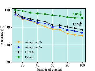
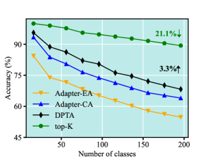
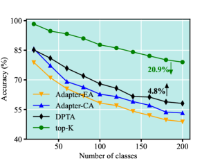
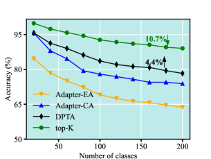
[CIFAR] [CARS] [CUB]
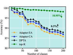
[ImageNet-A] [ImageNet-R] [VTAB]

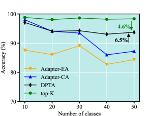
Figure 5: Ablation study results on six benchmark datasets, where the green annotation indicates the decrease in the final accuracy $A_{F}$ of DPTA over top-K prediction, and the black annotation denotes the improvement of DPTA over Adapter-CA.

5.3 Ablation Study

An ablation study is proposed in this subsection to investigate the effectiveness of the DPTA’s components on the six benchmarks above. The accuracy $A_{b}$ of the control group is reported in Figure 5, where the Adapter-CA uses the center-adapt loss of Eq.(6) and fine-tune the PTM with first-task adaption to assess the effectiveness of DPN. Adapter-EA uses the CE loss to fine-tune the PTM with first-task adaption, which is used to evaluate whether the center-adapt loss can improve classification accuracy. In addition, we provide top-K prediction accuracies to evaluate whether DPTA reaches its upper bound on performance. The results indicate that the accuracy of DPTA is significantly higher than group Adapter-CA, proving the effectiveness of DPN. Meanwhile, the comparison between the Adapter-CA and Adapter-EA groups illustrates that center-adapt loss can enhance the performance of prototype NCM classification.

5.4 Further Analysis of DPTA in Accuracy

[] []

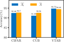
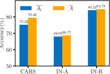
Figure 6: The $\overline{A_{t}}$ and $\overline{A}$ results on six datasets, where IN-A and IN-R denote the ImageNet-A and ImageNet-R datasets.

Even obtaining the SOTA performance, results in Figure 5 show that the accuracy of DPTA is far from the top-K prediction, which reveals the prediction of augmented prototypes has errors according to Eq.(4.3). To explore the causes, we counted each fine-tuning accuracy $A_{t}$ on the test set of task $t$ and the average $\overline{A_{t}}$, which is reported in Figure 6 along with $\overline{A}$. As illustrated, the gap between $\overline{A_{t}}$ and $\overline{A}$ is small, indicating that the augmented prototypes’ error mainly comes from the limited task adaption. Specifically, several on-task samples in the subspace are hard to separate, and even fine-tuning the PTM by adapters with center-adapt loss is not enough. For example, in Figure 3, a few black samples are mixed in the green clusters. At this point, increasing the number of top-K may not improve accuracy either. It is only necessary to ensure the accuracy of top-K labels is significantly higher than $\overline{A_{t}}$, and improving the performance of DPTA should focus on the augmented prototype construction, such as utilizing better fine-tuning modules and loss functions. In the supplementary material, we present additional experiments with respect to hyper-parameter K and provide several tricks dedicated to DPTA that may help boost its performance.

6 Conclusion

In real-world applications, we expect machine learning models to learn from streaming data without forgetting. This paper proposes the dual prototype network with task-wise adaption (DPTA) for pre-trained model-based class-incremental learning. We train task-wise adapters for PTM using the center-adapt loss, to make the representation extracted by PTM more class discriminative. The appropriate adapters for each test sample are selected through raw prototypes, and a better prediction is made through task-wise augmented prototypes. Various experiments have proven DPTA’s excellent performance. However, the accuracy of DPTA is still far from its upper bound. Our future work will focus on improving the $K$-class classification accuracy using augmented prototypes.

References

- Ahn et al. [2019] Hongjoon Ahn, Sungmin Cha, Donggyu Lee, and Taesup Moon. Uncertainty-based continual learning with adaptive regularization. Advances in neural information processing systems, 32, 2019.
- Barbu et al. [2019] Andrei Barbu, David Mayo, Julian Alverio, William Luo, Christopher Wang, Dan Gutfreund, Josh Tenenbaum, and Boris Katz. Objectnet: A large-scale bias-controlled dataset for pushing the limits of object recognition models. Advances in neural information processing systems, 32, 2019.
- Bezdek and Kuncheva [2001] James C Bezdek and Ludmila I Kuncheva. Nearest prototype classifier designs: An experimental study. International journal of Intelligent systems, 16(12):1445–1473, 2001.
- Chen et al. [2021] Shuo Chen, Gang Niu, Chen Gong, Jun Li, Jian Yang, and Masashi Sugiyama. Large-margin contrastive learning with distance polarization regularizer. In International Conference on Machine Learning, pages 1673–1683. PMLR, 2021.
- Chen et al. [2022] Shuo Chen, Chen Gong, Jun Li, Jian Yang, Gang Niu, and Masashi Sugiyama. Learning contrastive embedding in low-dimensional space. Advances in Neural Information Processing Systems, 35:6345–6357, 2022.
- De Lange and Tuytelaars [2021] Matthias De Lange and Tinne Tuytelaars. Continual prototype evolution: Learning online from non-stationary data streams. In Proceedings of the IEEE/CVF international conference on computer vision, pages 8250–8259, 2021.
- De Lange et al. [2021] Matthias De Lange, Rahaf Aljundi, Marc Masana, Sarah Parisot, Xu Jia, Aleš Leonardis, Gregory Slabaugh, and Tinne Tuytelaars. A continual learning survey: Defying forgetting in classification tasks. IEEE transactions on pattern analysis and machine intelligence, 44(7):3366–3385, 2021.
- Deng et al. [2009] Jia Deng, Wei Dong, Richard Socher, Li-Jia Li, Kai Li, and Li Fei-Fei. Imagenet: A large-scale hierarchical image database. In 2009 IEEE conference on computer vision and pattern recognition, pages 248–255. Ieee, 2009.
- Dosovitskiy [2020] Alexey Dosovitskiy. An image is worth 16x16 words: Transformers for image recognition at scale. arXiv preprint arXiv:2010.11929, 2020.
- French [1999] Robert M French. Catastrophic forgetting in connectionist networks. Trends in cognitive sciences, 3(4):128–135, 1999.
- Gomes et al. [2017] Heitor Murilo Gomes, Jean Paul Barddal, Fabrício Enembreck, and Albert Bifet. A survey on ensemble learning for data stream classification. ACM Computing Surveys (CSUR), 50(2):1–36, 2017.
- Hendrycks et al. [2021a] Dan Hendrycks, Steven Basart, Norman Mu, Saurav Kadavath, Frank Wang, Evan Dorundo, Rahul Desai, Tyler Zhu, Samyak Parajuli, Mike Guo, et al. The many faces of robustness: A critical analysis of out-of-distribution generalization. In Proceedings of the IEEE/CVF international conference on computer vision, pages 8340–8349, 2021a.
- Hendrycks et al. [2021b] Dan Hendrycks, Kevin Zhao, Steven Basart, Jacob Steinhardt, and Dawn Song. Natural adversarial examples. In Proceedings of the IEEE/CVF conference on computer vision and pattern recognition, pages 15262–15271, 2021b.
- Houlsby et al. [2019] Neil Houlsby, Andrei Giurgiu, Stanislaw Jastrzebski, Bruna Morrone, Quentin De Laroussilhe, Andrea Gesmundo, Mona Attariyan, and Sylvain Gelly. Parameter-efficient transfer learning for nlp. In International conference on machine learning, pages 2790–2799. PMLR, 2019.
- Jaimes and Sebe [2007] Alejandro Jaimes and Nicu Sebe. Multimodal human–computer interaction: A survey. Computer vision and image understanding, 108(1-2):116–134, 2007.
- Jia et al. [2022] Menglin Jia, Luming Tang, Bor-Chun Chen, Claire Cardie, Serge Belongie, Bharath Hariharan, and Ser-Nam Lim. Visual prompt tuning. In European Conference on Computer Vision, pages 709–727. Springer, 2022.
- Kramberger and Potočnik [2020] Tin Kramberger and Božidar Potočnik. Lsun-stanford car dataset: enhancing large-scale car image datasets using deep learning for usage in gan training. Applied Sciences, 10(14):4913, 2020.
- Krizhevsky et al. [2009] Alex Krizhevsky, Geoffrey Hinton, et al. Learning multiple layers of features from tiny images. Technical report, 2009.
- Krizhevsky et al. [2012] Alex Krizhevsky, Ilya Sutskever, and Geoffrey E Hinton. Imagenet classification with deep convolutional neural networks. Advances in neural information processing systems, 25, 2012.
- Li and Yuan [2017] Yuanzhi Li and Yang Yuan. Convergence analysis of two-layer neural networks with relu activation. Advances in neural information processing systems, 30, 2017.
- Li and Hoiem [2017] Zhizhong Li and Derek Hoiem. Learning without forgetting. IEEE transactions on pattern analysis and machine intelligence, 40(12):2935–2947, 2017.
- Lian et al. [2022] Dongze Lian, Daquan Zhou, Jiashi Feng, and Xinchao Wang. Scaling & shifting your features: A new baseline for efficient model tuning. Advances in Neural Information Processing Systems, 35:109–123, 2022.
- Liu et al. [2015] Ziwei Liu, Ping Luo, Xiaogang Wang, and Xiaoou Tang. Deep learning face attributes in the wild. In Proceedings of the IEEE international conference on computer vision, pages 3730–3738, 2015.
- Lopez-Paz and Ranzato [2017] David Lopez-Paz and Marc’Aurelio Ranzato. Gradient episodic memory for continual learning. Advances in neural information processing systems, 30, 2017.
- Mallya et al. [2018] Arun Mallya, Dillon Davis, and Svetlana Lazebnik. Piggyback: Adapting a single network to multiple tasks by learning to mask weights. In Proceedings of the European conference on computer vision (ECCV), pages 67–82, 2018.
- Masana et al. [2022] Marc Masana, Xialei Liu, Bartłomiej Twardowski, Mikel Menta, Andrew D Bagdanov, and Joost Van De Weijer. Class-incremental learning: survey and performance evaluation on image classification. IEEE Transactions on Pattern Analysis and Machine Intelligence, 45(5):5513–5533, 2022.
- McDonnell et al. [2024] Mark D McDonnell, Dong Gong, Amin Parvaneh, Ehsan Abbasnejad, and Anton van den Hengel. Ranpac: Random projections and pre-trained models for continual learning. Advances in Neural Information Processing Systems, 36, 2024.
- Nguyen et al. [2017] Cuong V Nguyen, Yingzhen Li, Thang D Bui, and Richard E Turner. Variational continual learning. arXiv preprint arXiv:1710.10628, 2017.
- Panos et al. [2023] Aristeidis Panos, Yuriko Kobe, Daniel Olmeda Reino, Rahaf Aljundi, and Richard E Turner. First session adaptation: A strong replay-free baseline for class-incremental learning. In Proceedings of the IEEE/CVF International Conference on Computer Vision, pages 18820–18830, 2023.
- Paszke et al. [2019] Adam Paszke, Sam Gross, Francisco Massa, Adam Lerer, James Bradbury, Gregory Chanan, Trevor Killeen, Zeming Lin, Natalia Gimelshein, Luca Antiga, et al. Pytorch: An imperative style, high-performance deep learning library. Advances in neural information processing systems, 32, 2019.
- Radford et al. [2021] Alec Radford, Jong Wook Kim, Chris Hallacy, Aditya Ramesh, Gabriel Goh, Sandhini Agarwal, Girish Sastry, Amanda Askell, Pamela Mishkin, Jack Clark, et al. Learning transferable visual models from natural language supervision. In International conference on machine learning, pages 8748–8763. PMLR, 2021.
- Rebuffi et al. [2017] Sylvestre-Alvise Rebuffi, Alexander Kolesnikov, Georg Sperl, and Christoph H Lampert. icarl: Incremental classifier and representation learning. In Proceedings of the IEEE conference on Computer Vision and Pattern Recognition, pages 2001–2010, 2017.
- Rolnick et al. [2019] David Rolnick, Arun Ahuja, Jonathan Schwarz, Timothy Lillicrap, and Gregory Wayne. Experience replay for continual learning. Advances in neural information processing systems, 32, 2019.
- Serra et al. [2018] Joan Serra, Didac Suris, Marius Miron, and Alexandros Karatzoglou. Overcoming catastrophic forgetting with hard attention to the task. In International conference on machine learning, pages 4548–4557. PMLR, 2018.
- Shafer [1985] Glenn Shafer. Conditional probability. International Statistical Review/Revue Internationale de Statistique, pages 261–275, 1985.
- Simon et al. [2021] Christian Simon, Piotr Koniusz, and Mehrtash Harandi. On learning the geodesic path for incremental learning. In Proceedings of the IEEE/CVF conference on Computer Vision and Pattern Recognition, pages 1591–1600, 2021.
- Smith et al. [2023] James Seale Smith, Leonid Karlinsky, Vyshnavi Gutta, Paola Cascante-Bonilla, Donghyun Kim, Assaf Arbelle, Rameswar Panda, Rogerio Feris, and Zsolt Kira. Coda-prompt: Continual decomposed attention-based prompting for rehearsal-free continual learning. In Proceedings of the IEEE/CVF Conference on Computer Vision and Pattern Recognition, pages 11909–11919, 2023.
- Sun et al. [2023] Hai-Long Sun, Da-Wei Zhou, Han-Jia Ye, and De-Chuan Zhan. Pilot: A pre-trained model-based continual learning toolbox. arXiv preprint arXiv:2309.07117, 2023.
- Tao et al. [2020] Xiaoyu Tao, Xinyuan Chang, Xiaopeng Hong, Xing Wei, and Yihong Gong. Topology-preserving class-incremental learning. In Computer Vision–ECCV 2020: 16th European Conference, Glasgow, UK, August 23–28, 2020, Proceedings, Part XIX 16, pages 254–270. Springer, 2020.
- Van der Maaten and Hinton [2008] Laurens Van der Maaten and Geoffrey Hinton. Visualizing data using t-sne. Journal of machine learning research, 9(11), 2008.
- Wah et al. [2011] Catherine Wah, Steve Branson, Peter Welinder, Pietro Perona, and Serge Belongie. The caltech-ucsd birds-200-2011 dataset. Technical Report CNS-TR-2011-001, 2011.
- Wang et al. [2022a] Fu-Yun Wang, Da-Wei Zhou, Han-Jia Ye, and De-Chuan Zhan. Foster: Feature boosting and compression for class-incremental learning. In European conference on computer vision, pages 398–414. Springer, 2022a.
- Wang et al. [2024] Liyuan Wang, Xingxing Zhang, Hang Su, and Jun Zhu. A comprehensive survey of continual learning: theory, method and application. IEEE Transactions on Pattern Analysis and Machine Intelligence, 2024.
- Wang et al. [2022b] Yabin Wang, Zhiwu Huang, and Xiaopeng Hong. S-prompts learning with pre-trained transformers: An occam’s razor for domain incremental learning. Advances in Neural Information Processing Systems, 35:5682–5695, 2022b.
- Wang et al. [2023] Yabin Wang, Zhiheng Ma, Zhiwu Huang, Yaowei Wang, Zhou Su, and Xiaopeng Hong. Isolation and impartial aggregation: A paradigm of incremental learning without interference. In Proceedings of the AAAI Conference on Artificial Intelligence, pages 10209–10217, 2023.
- Wang et al. [2022c] Zifeng Wang, Zizhao Zhang, Sayna Ebrahimi, Ruoxi Sun, Han Zhang, Chen-Yu Lee, Xiaoqi Ren, Guolong Su, Vincent Perot, Jennifer Dy, et al. Dualprompt: Complementary prompting for rehearsal-free continual learning. In European Conference on Computer Vision, pages 631–648. Springer, 2022c.
- Wang et al. [2022d] Zifeng Wang, Zizhao Zhang, Chen-Yu Lee, Han Zhang, Ruoxi Sun, Xiaoqi Ren, Guolong Su, Vincent Perot, Jennifer Dy, and Tomas Pfister. Learning to prompt for continual learning. In Proceedings of the IEEE/CVF conference on computer vision and pattern recognition, pages 139–149, 2022d.
- Wen et al. [2016] Yandong Wen, Kaipeng Zhang, Zhifeng Li, and Yu Qiao. A discriminative feature learning approach for deep face recognition. In Computer vision–ECCV 2016: 14th European conference, amsterdam, the netherlands, October 11–14, 2016, proceedings, part VII 14, pages 499–515. Springer, 2016.
- Xu and Zhu [2018] Ju Xu and Zhanxing Zhu. Reinforced continual learning. Advances in neural information processing systems, 31, 2018.
- Xu et al. [2020] Wenjia Xu, Yongqin Xian, Jiuniu Wang, Bernt Schiele, and Zeynep Akata. Attribute prototype network for zero-shot learning. Advances in Neural Information Processing Systems, 33:21969–21980, 2020.
- Yan et al. [2021] Shipeng Yan, Jiangwei Xie, and Xuming He. Der: Dynamically expandable representation for class incremental learning. In Proceedings of the IEEE/CVF conference on computer vision and pattern recognition, pages 3014–3023, 2021.
- Yang et al. [2018] Hong-Ming Yang, Xu-Yao Zhang, Fei Yin, and Cheng-Lin Liu. Robust classification with convolutional prototype learning. In Proceedings of the IEEE conference on computer vision and pattern recognition, pages 3474–3482, 2018.
- Yang et al. [2002] Ming-Hsuan Yang, David J Kriegman, and Narendra Ahuja. Detecting faces in images: A survey. IEEE Transactions on pattern analysis and machine intelligence, 24(1):34–58, 2002.
- Ye et al. [2019] Han-Jia Ye, De-Chuan Zhan, Nan Li, and Yuan Jiang. Learning multiple local metrics: Global consideration helps. IEEE transactions on pattern analysis and machine intelligence, 42(7):1698–1712, 2019.
- Yu et al. [2020] Lu Yu, Bartlomiej Twardowski, Xialei Liu, Luis Herranz, Kai Wang, Yongmei Cheng, Shangling Jui, and Joost van de Weijer. Semantic drift compensation for class-incremental learning. In Proceedings of the IEEE/CVF conference on computer vision and pattern recognition, pages 6982–6991, 2020.
- Zeno et al. [2018] Chen Zeno, Itay Golan, Elad Hoffer, and Daniel Soudry. Task agnostic continual learning using online variational bayes. arXiv preprint arXiv:1803.10123, 2018.
- Zhai et al. [2019] Xiaohua Zhai, Joan Puigcerver, Alexander Kolesnikov, Pierre Ruyssen, Carlos Riquelme, Mario Lucic, Josip Djolonga, Andre Susano Pinto, Maxim Neumann, Alexey Dosovitskiy, et al. A large-scale study of representation learning with the visual task adaptation benchmark. arXiv preprint arXiv:1910.04867, 2019.
- Zhang et al. [2020] Junting Zhang, Jie Zhang, Shalini Ghosh, Dawei Li, Serafettin Tasci, Larry Heck, Heming Zhang, and C-C Jay Kuo. Class-incremental learning via deep model consolidation. In Proceedings of the IEEE/CVF winter conference on applications of computer vision, pages 1131–1140, 2020.
- Zhang and Sabuncu [2018] Zhilu Zhang and Mert Sabuncu. Generalized cross entropy loss for training deep neural networks with noisy labels. Advances in neural information processing systems, 31, 2018.
- Zhou et al. [2022] Da-Wei Zhou, Qi-Wei Wang, Han-Jia Ye, and De-Chuan Zhan. A model or 603 exemplars: Towards memory-efficient class-incremental learning. arXiv preprint arXiv:2205.13218, 2022.
- Zhou et al. [2024a] Da-Wei Zhou, Zi-Wen Cai, Han-Jia Ye, De-Chuan Zhan, and Ziwei Liu. Revisiting class-incremental learning with pre-trained models: Generalizability and adaptivity are all you need. International Journal of Computer Vision, pages 1–21, 2024a.
- Zhou et al. [2024b] Da-Wei Zhou, Hai-Long Sun, Jingyi Ning, Han-Jia Ye, and De-Chuan Zhan. Continual learning with pre-trained models: A survey. arXiv preprint arXiv:2401.16386, 2024b.
- Zhou et al. [2024c] Da-Wei Zhou, Hai-Long Sun, Han-Jia Ye, and De-Chuan Zhan. Expandable subspace ensemble for pre-trained model-based class-incremental learning. In Proceedings of the IEEE/CVF Conference on Computer Vision and Pattern Recognition, pages 23554–23564, 2024c.
- Zhou et al. [2024d] Da-Wei Zhou, Qi-Wei Wang, Zhi-Hong Qi, Han-Jia Ye, De-Chuan Zhan, and Ziwei Liu. Class-incremental learning: A survey. IEEE Transactions on Pattern Analysis and Machine Intelligence, 2024d.