Constraining symmetron fields with a levitated optomechanical system

Abstract

The symmetron, one of the light scalar fields introduced by dark energy theories, is thought to modify the gravitational force when it couples to matter. However, detecting the symmetron field is challenging due to its screening behavior in the high-density environment of traditional measurements. In this paper, we propose a scheme to set constraints on the parameters of the symmetron with a levitated optomechanical system, in which a nanosphere serves as a testing mass coupled to an optical cavity. By measuring the frequency shift of the probe transmission spectrum, we can establish constraints for our scheme by calculating the symmetron-induced influence. These refined constraints improve by 1 to 3 orders of magnitude compared to current force-based detection methods, which offer new opportunities for the dark energy detection.

1 Introduction

Observations on the cosmic scale have indicated an accelerating expansion of our universe, but a convincing explanation of this phenomenon remains elusive[1, 2, 3]. A critical issue is that there is a discrepancy between different measurements of Hubble constant $H_{0}$ [4, 5, 6, 7]. The Planck satellite gives the value $H_{0}=(67.8\pm 0.5)$km/s$\cdot$Mpc[8] while the SH0ES team result indicates $H_{0}=(73.0\pm 1.0)$km/s$\cdot$Mpc[9]. Common explanations include simply systematic errors, underdensity-area-induced expansion acceleration[10, 11] and new physics beyond the standard model[12, 13]. However, the first explanation fails because the disagreement is sufficiently large across different statistical approaches [14, 15] and the second one is ruled out by observations[16]. The most popular answer seems to be dark energy, where the acceleration of expansion is explained within the framework of the scalar field[17]. Additionally, high energy physics theories suggest that the coupling between the scalar field and matter results in the so-called fifth force beyond the four fundamental forces, which leads to the modification of the gravitational force [18].

Considering the fact that the scalar fields evade the search in local environment, there must be a screening mechanism to shield them from laboratory detection[19]. Several types of screening mechanism have been proposed, including the chameleon[20, 21], the symmetron[22, 23], K-mouflage[24] and Vainshtein[25]. Among what is discussed above, the former two share a unified description but different Lagrangians. They both mediate long-range forces in low density areas. But in high density areas, the mass of the chameleon increases and the mediated force become short-range[20], while the symmetron develops nonlinearity that results in its decoupling from matter[26]. In contrast, the latter two are mainly determined by the steep field gradients of the scalar field and the second derivative of the field, respectively[27, 28, 29].

Here, we focus on the symmetron model. To be specific, the symmetron model relies on the vacuum expectation value of a scalar field , which undergoes a $\mathbb{Z}_{2}$ symmetry breaking transition as the local matter density decreases from a critical value[30, 31, 32]. In contrast, when the matter density is large, the effective field potential has only one minimum and remains zero. There have been several tests and related analyses of constraints on the symmetron field, including satellite-based tests[33] , torsion pendulum experiments[34, 35], Casimir-force detection[36, 37, 29], neutron tests[38, 39] and atomic interferometry[20, 40]. With the results of the mentioned tests, the physically plausible parameter space has been covered by considering different constraints[30, 41].

In this paper, we propose a scheme aimed for probing the symmetron-force gradient with an optically trapped nanosphere for future experiments. The article is organized as follows: In Sec. 2, we present the theoretical model, including a brief introduction of symmetron field as well as a solution considering the screening mechanism. We also derive the relation between the symmetron force gradient and the force-induced frequency shift via quantum optics theory. In Sec. 3, we determine the minimum measurable frequency shift, considering the spectroscopic performance and dominant noise processes. Additionally, we establish the constraints on symmetron through the aforementioned calculation and demonstrate an improvement of 3 to 1 orders of magnitude for $\mu$ in the range $10^{-1}$eV to $10^{-4}$eV. In Sec. 4, we summarize the paper and discuss potential future research directions.

2 Model and theory

2.1 The cavity optomechanical system

Our scheme is based on a system shown in Fig. 1, composed of a fused silica sphere trapped in an optical cavity with resonance frequency $\omega_{cav}$. we utilized a pump light field with frequency $\omega_{p}$ and a weak probe field with frequency $\omega_{s}$[42, 43, 44]. Generally, we have the Hamiltonian of the entire system in a rotating frame given by [45, 46]

$$H=\hbar\Delta_{p}c^{\dagger}c+\hbar\omega_{n}a^{\dagger}a-\hbar gc^{\dagger}c(a^{\dagger}+a)-i\hbar\Omega_{p}(c-c^{\dagger})-i\hbar\Omega_{s}(ce^{i\delta t}-c^{\dagger}e^{-i\delta t}),$$ (2.1)

where $\Delta_{p}=\omega_{cav}-\omega_{p}$ is pump-cavity detuning which we set to $\Delta_{p}=0$ for the this paper; $c(c^{\dagger})$ and $a(a^{\dagger})$ denote the annihilation (creation) operator of the cavity and the bosonic annihilation (creation) operator of the quantum harmonic oscillator; the interaction term $H_{\text{int}}=\hbar gc^{\dagger}c(a+a^{\dagger})$ describes the coupling between the cavity and the oscillation of the trapped particle with the coupling strength $g$; $\delta=\omega_{s}-\omega_{p}$ is the probe-pump detuning; $\Omega_{p}$ and $\Omega_{s}$ are the Rabi frequency for the pump field and the probe field in the cavity respectively, which are proportional to $\sqrt{P_{p}}$ and $\sqrt{P_{s}}$. Here $P_{p}$ and $P_{s}$ are the power of the pump field and the probe field.

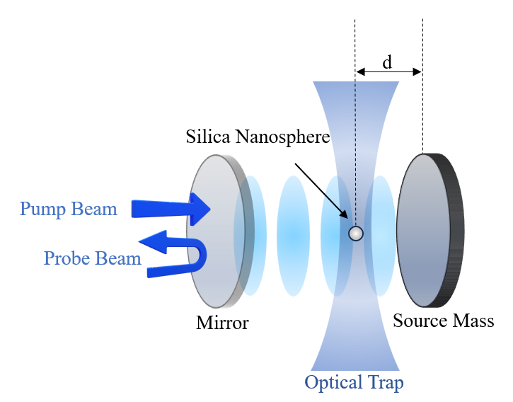
Figure 1: The schematic diagram of our system which consists of an optically trapped fused silica nanosphere driven by a pump beam and a weak probe laser, with radius $R=100$nm and density $\rho_{sphere}=2.2\times 10^{3}$kg$/m^{3}$. The system includes a transflective mirror as well as another mirror served as source mass. The sphere is cooled in the cavity and positioned at a distance $d$ from the source mass surface.

Moreover, the system measures the force gradient with the optomechanical setup as follows: When under a uniform force, the nanosphere experiences a harmonic trapping potential with spring constant $k$ defined by $\omega_{n}=\sqrt{k/m}$, where $\omega_{n}$ is the resonance frequency. However, when it experiences a non-vanishing force gradient, the spring constant is modified to $k^{\prime}=k+\partial F/\partial x$, leading to a change of frequency

$$\omega^{\prime}_{n}\approx\sqrt{\frac{k}{m}\left(1+\frac{\partial F/\partial x}{k}\right)}.$$ (2.2)

Given $\omega_{n}\approx\omega^{\prime}_{n}$,we have

$$\frac{\partial F/\partial x}{2k}\approx\frac{\omega^{\prime}_{n}}{\omega_{n}}-1,$$ (2.3)

and the relation between the frequency shift $\Delta\omega$ and the force gradient $\frac{\partial F}{\partial x}$ is

$$\frac{\partial F}{\partial x}=\frac{2k\Delta\omega}{\omega_{n}}.$$ (2.4)

Then we define the operator $N=a+a^{\dagger}$, which is related to the position of the quantum oscillator. Using the Heisenberg equation and the communication relations that $[c,c^{\dagger}]=1$ and $[a,a^{\dagger}]=1$, we have the evolution of $c$ and $N$ described by the quantum Langevin equations with additional damping terms:

$$\frac{dc}{dt}=-(i\Delta_{p}+\kappa)c+igNc+\Omega_{p}+\Omega_{s}e^{-i\omega t}+\sqrt{\kappa_{ex}}\hat{a}_{in}+\sqrt{\kappa_{0}}\hat{f}_{in},$$ (2.5)

$$\frac{d^{2}N}{dt^{2}}+\gamma_{n}\frac{dN}{dt}+\omega_{n}^{2}N=2\omega_{n}gc^{\dagger}c+\hat{\xi},$$ (2.6)

here $\kappa=\kappa_{0}+\kappa_{\text{ex}}$ and $\gamma_{n}$ are the energy damping rate of the cavity and the damping rates of the vibrational mode of the nanosphere, respectively. $\hat{a}_{\text{in}}(t)$ is the Langevin noise operator, which has mean value of $\langle\hat{a}_{\text{in}}(t)\rangle=0$ with correlation function written as $\langle\hat{a}_{\text{in}}(t)\hat{a}_{\text{in}}(t_{0})\rangle\sim\delta(t-t_{0})$. And $\hat{f}$ has similar form of correlators as those for $\hat{a}_{\text{in}}$. The operator $\hat{\xi}$ stands for the effects of the thermal bath from the non-Markovian stochastic process and the Brownian. It also has a zero mean value with correlation function is given by[46, 47]

$$\left\langle\hat{\xi(t)^{\dagger}}\hat{\xi(t^{\prime})}\right\rangle=\frac{\gamma_{n}}{\omega_{n}}\int\frac{d\omega}{2\pi}\omega e^{-i\omega(t-t^{\prime})}\left[1+\coth\left(\frac{\hbar\omega}{2k_{B}T}\right)\right],$$ (2.7)

where $k_{B}$ is the Boltzmann’s constant and $T$ is the effective resonator temperature. Each Heisenberg operator can be separated into its steady-state and fluctuation part:

$$c=c_{0}+\delta c,$$ (2.8)

$$N=N_{0}+\delta N.$$ (2.9)

Then we can get the steady-state solutions of Eqs. (2.5) and (2.6) as

$$c_{0}=\frac{\Omega_{p}}{(i\Delta_{pu}+\kappa)-igN},$$ (2.10)

$$N_{0}=\frac{2g|c|^{2}}{\omega_{n}}.$$ (2.11)

Taking Eqs. (2.10)and (2.11) into the Langevin equations, one can get the linearized Langevin equations by dropping the noise terms and nonlinear terms since we choose a weak driving field.

$$\langle\delta\dot{c}\rangle=-\kappa\langle\delta c\rangle+ig(N_{0}\langle\delta c\rangle+c_{0}\langle\delta N\rangle)+\Omega_{p}+\Omega_{s}e^{-i\delta t},$$ (2.12)

$$\langle\delta\ddot{N}\rangle+\gamma_{n}\langle\delta\dot{N}\rangle+\omega^{2}_{n}\langle\delta N\rangle=2\omega_{n}gc^{2}_{0}.$$ (2.13)

To solve these equations, we introduce the following ansatz[48]:

$$\langle\delta c\rangle=c_{+}e^{-i\delta t}+c_{-}e^{i\delta t},$$ (2.14)

$$\langle\delta N\rangle=N_{+}e^{-i\delta t}+N_{-}e^{i\delta t}.$$ (2.15)

By substituting these expressions into the Eqs. (2.5) and (2.6), we obtain the solutions of interest:

$$c_{+}=\frac{\Omega_{s}[B(E-P)+G\omega_{0}]}{B(E^{2}-P^{2})+2PG\omega_{0}},$$ (2.16)

$$\Omega^{2}_{p}=\omega_{0}(\kappa^{2}+(\Delta_{p}-g^{2}\omega_{0}/\omega_{n})^{2}).$$ (2.17)

The parameters in the above equations are given as follows:$E=\kappa-i\delta$, $P=i\Delta p-igN_{0}$, $B=-\delta^{2}-i\gamma_{n}\delta+\omega_{n}^{2}$, $G=2ig^{2}\omega_{n}$, $N_{0}=2g|c_{0}|^{2}/\omega_{n}$, and $\omega_{0}=|c_{0}|^{2}$ can be resolved by Eq. (2.17). Here $c_{+}$ is a parameter analogous to the linear optical susceptibility. Its real part and imaginary part exhibit absorptive and dispersive behavior, which can be observed by detecting the transmission spectrum of the probe field.

To calculate the transmission of the probe field, we first calculate the mean value of output field by using the input-output relation

$$c_{\text{out}}(t)=c_{\text{in}}(t)-\sqrt{2\kappa}c(t),$$ (2.18)

where $c_{\text{in}}$ and $c_{\text{out}}$ are the input and output operators; thus, we can obtain the expectation value of the output field as[49]:

$$\langle c_{out}(t)\rangle=(\frac{\Omega_{p}}{\sqrt{2\kappa}}-\sqrt{2\kappa}c_{0})e^{-i\omega_{p}t}+(\frac{\Omega_{s}}{\sqrt{2\kappa}}-\sqrt{2\kappa}c_{+})e^{-i(\omega_{p}+\delta)t}-\sqrt{2\kappa}c_{-}e^{-i(\omega_{p}-\delta)t}.$$ (2.19)

Focus on the component with frequency $\omega_{p}+\delta=\omega_{s}$, we deduce the transmission of the probe field, defined as the ratio of the output field and input field at the probe frequency:

$$\mathcal{T}(\omega_{s})=\frac{\Omega_{s}/\sqrt{2\kappa}-\sqrt{2\kappa}c_{+}}{\Omega_{s}/\sqrt{2\kappa}}.$$ (2.20)

2.2 The symmetron force

First of all, we have the Lagrangian density of the symmetron field in natural unit($c=\hbar=1$)

$$\mathcal{L}=-\frac{1}{2}(\partial\phi)^{2}-\frac{1}{2}(\frac{\rho}{M^{2}}-\mu^{2})\phi^{2}-\frac{1}{4}\lambda\phi^{4}-\frac{\mu^{4}}{4\lambda}.$$ (2.21)

The parameters in the above equation have the following meanings: $\mu$, serves as the tachyonic mass; $\lambda$ is a dimensionless self-coupling constant; and $M$ is a parameter characterizing the coupling strength to matter with the dimension of mass. Considering the interaction with background matter of density $\rho$, we get a $\mathbb{Z}_{2}$ symmetry breaking potential as

$$V_{eff}(\phi)=\frac{1}{2}(\frac{\rho}{M^{2}}-\mu^{2})\phi^{2}+\frac{1}{4}\lambda\phi^{4}+\frac{\mu^{4}}{4\lambda}.$$ (2.22)

It’s obvious that there is only one minimum of the effective potential at $\phi=0$ when the background matter density is higher than the critical value $\rho_{\text{crit}}=\mu^{2}M^{2}$. In contrast, as the matter density decreases to 0, the minima of the effective potential split into two values at $\phi_{\text{min}}=\pm{v}$ with $v=\mu/\sqrt{\lambda}$. According to the nature of symmetron field that it has two minima for effective potential, a unique phenomenon occurs which is not present in other chameleon models. if the Compton wavelength is smaller than the size of the vacuum cavity, it would be possible for the symmetron field to form a domain wall during the process pumping out the air from the cavity[30]. It is because that the field appears to emerge at either minimum with the equal probability. Here, we only consider the positive value, and then we can get the equation of motion and the force which a test matter $m_{test}$ in the symmetron field experiences with Eq. (2.22)

$$\vec{\nabla}^{2}\phi=(\frac{\rho}{M^{2}}-\mu^{2})\phi+\lambda\phi^{3},$$ (2.23)

$$F=-\frac{m_{test}}{M^{2}}\phi\vec{\nabla}\phi.$$ (2.24)

To solve the equation of motion , we consider a monotonically rising field towards the vacuum expectation value as follows(see refs. [50, 51, 52] for detailed treatment):

$$\phi(x)=v\tanh(\frac{\mu x}{\sqrt{2}}),$$ (2.25)

where $x$ is the distance from the surface of the plate to the center of the sphere.

In our scheme, we utilize a sphere-plate system, in which we should consider the so-called screening factor $\lambda_{sphere}$ for the nanosphere we use here.The screening factor characterizes the behavior of the symmetron field when the matter is sufficiently large or dense that $\rho\geq\mu^{2}M^{2}$. In that case, the interaction is proportional to only a small fraction $\lambda_{sphere}\ll 1$ of the whole matter. So the Eq. (2.24) is modified by replacing $m_{test}$ with $\lambda_{sphere}m_{test}$ [53]

$$F=-\frac{\lambda_{sphere}m_{test}}{M^{2}}\phi\vec{\nabla}\phi.$$ (2.26)

where we introduce the screening factor for a sphere with radius $R$ as[29]

$$\lambda_{sphere}\approx min(\frac{3M^{2}}{\rho R^{2}},1).$$ (2.27)

The above form of $\lambda$ allows the force to have a non-vanishing prefactor at the limit when $\lambda_{sphere}\rightarrow 0$ as

$$\frac{\lambda_{sphere}m_{sphere}}{M^{2}}=4\pi R.$$ (2.28)

Take Eqs. (2.25) and (2.28) into Eq.( 2.26), the symmetron force and its gradient can be written as

$$F=-\frac{4\pi v^{2}\mu R}{\sqrt{2}}\tanh(\frac{\mu x}{\sqrt{2}})\operatorname{sech}^{2}(\frac{\mu x}{\sqrt{2}}),$$ (2.29)

$$\frac{\partial F}{\partial x}=\frac{2\pi\mu^{4}R}{\lambda}\left(3\tanh^{2}\frac{\mu x}{\sqrt{2}}-1\right)\operatorname{sech}^{2}\left(\frac{\mu x}{\sqrt{2}}\right).$$ (2.30)

It should be emphasized that the density of the sphere and mirrors is sufficiently large, so the symmetron field is zero everywhere inside these objects. Therefore, we focus only on the nonvanishing field in the vacuum.

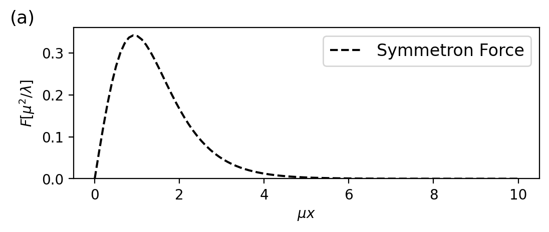
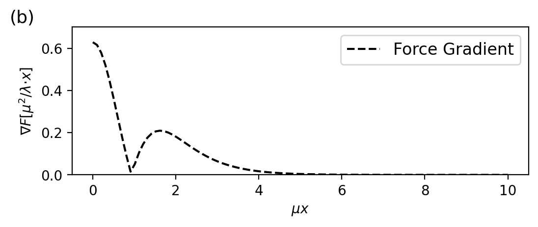
Figure 2: The symmetron force (a) and the force gradient(b) plotted as functions of the distance from the plate to the sphere. To be convenient, we choose $\mu^{2}/\lambda$ and $\mu^{2}/\lambda\cdot x$ as dimension, respectively. The criteria of small ball is $\mu R\ll 1$, by which we can ignore influence of sphere on the symmetron field from the plate. Here, we choose $\mu R$=0.1 to give an example of the symmetron mechanism.

In Fig. 2, we plot the symmetron force and its force gradient as functions of the distance from the plate to the sphere. It can be found that the force approaches zero as the sphere get closer to the plate. This phenomena is in good agreement with the quadratic coupling of the symmetron to matter. A sensitive force gradient detection would be achieved if we trap the sphere in a relatively closed location, since the value of gradient would be higher.

3 Numerical results

3.1 The detection of the frequency shift

In this section, we aim to present practical parameters and numerical results for the predicted cavity detection. Initially, we set the pump-cavity detuning $\Delta_{p}=\omega_{cav}-\omega_{p}=0$ for convenience. For the optical setup, we choose the trapping laser beam at the power P=0.17W with the wavelength $\lambda_{\text{{laser}}}=1064$nm injected into a cavity [54]. The pump beam is set to a power P=13nW at the frequency $\omega_{p}=2\pi\times 4.77$GHz [55].The cavity in our scheme is chosen to have an optical quality factor $Q\sim 10^{10}$ [56] with cavity amplitude decay rate $\kappa=2\pi\times 215$kHz [57]. Two mirrors of the cavity are considered to be separated by a distance L=2mm, with the mirror served as source mass being flat while the radius of curvature for the other mirror is $R_{\text{mirror}}=10\mu$m in reference to settings in ref. [58]. With the above parameters, the mode volume $V_{c}=1.09\times 10^{-13}$m³ can be calculated via $V_{c}\approx\pi Lw_{0}^{2}/4$, where $w_{0}$ is the waist for the fundamental mode. In addition, we can derive the coupling strength $g\sim 0.41$kHz with the following formula[59]

$$g=\frac{3}{4}\frac{V_{sphere}}{V_{c}}\frac{\epsilon-1}{\epsilon+2}\omega_{cav},$$ (3.1)

where $\epsilon=3.75$ is the relative permittivity for fused silica and $V_{sphere}=4.2\times 10^{-21}$m³ . Then we can derive the Rabi frequency for pump laser as $\Omega_{p}\approx 2\pi$MHz considering a power density $\approx 10$mW/cm² [60]. To achieve the mechanical damping rate, we choose a typical oscillator system with $\omega_{n}=2\pi\times 125$ kHz along the coupling direction [56], leading to a gas-induced decay damping rate $\Gamma_{n}\approx 7.98\times 10^{-7}$Hz decided by

$$\Gamma_{n}=\frac{16p}{\pi\bar{v}_{gas}R\rho_{sphere}},$$ (3.2)

where p=10^-10mbar is the gas pressure of vacuum cavity and mean velocity of gas is given by $\bar{v}_{gas}=\sqrt{k_{B}T/m_{gas}}\approx 290m/s$ [59, 58]. This allows the system to have a longer lifetime for potential operation, and this helps to ignore the effect of frequency drifts during measurement.

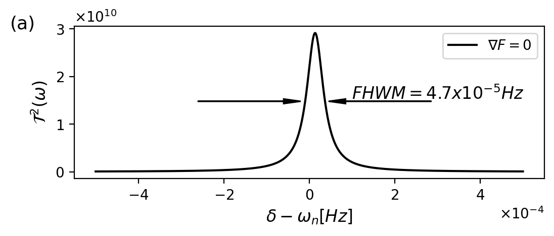
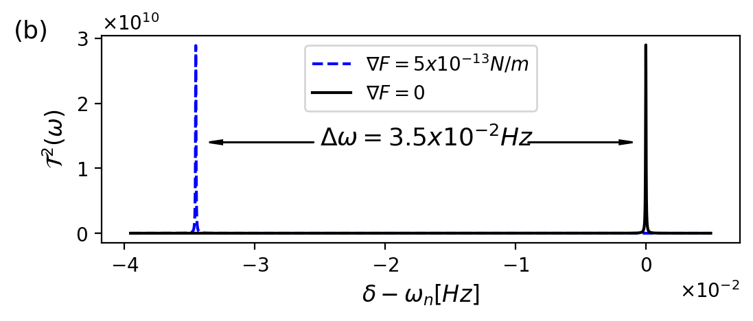
Figure 3: Transmission $\mathcal{T}^{2}{(\omega)}$ of the probe field as a function of $\delta-\omega_{n}$. (a) A sharp peak can be found at $\delta-\omega_{n}$ without the presence of external force gradient. Additionally, the FWHM=4.7$\times 10^{-5}$Hz is marked, representing the minimum distinguishable frequency discrepancy. (b) A frequency shift of $3.5\times 10^{-2}$Hz is observed from the black line(before) to the blue line(after) with a gradient of $5\times 10^{-13}$ N/m as an example.

To determine the ability of detection of our system, we should first investigate the probe spectrum through Eq. (2.20). Shown in Fig. 3, the peak is located at the original frequency $\delta=\omega_{n}$ in the condition that there is no the fifth-force gradient($\nabla F=0$). The resolution of the system depends on the full width at half maximum (FWHM) of the oscillation peak, which in our scheme can be measured as 4.7$\times 10^{-5}$Hz. Fig. 3 shows the impact of a nonzero force gradient on the spectrum. For instance, in the presence of a force gradient$\nabla F=5\times 10^{-13}$N/m, a frequency shift of $\Delta\omega=3.5\times 10^{-2}$Hz can be observed, which indicates that the effect of force gradient leads to a decrease of the resonance frequency. The relation between the frequency shift and force gradient is given by Eq. (2.4), by which we can derive the detection limit of our system is

$$\nabla F_{\text{min}}=\Delta\omega_{\text{FWHM}}\frac{2k}{\omega_{n}}=6.80\times 10^{-16}N/m,$$ (3.3)

with $m_{eff}=9.2\times 10^{-18}$kg and $k=m_{eff}\omega_{n}^{2}=5.68\times 10^{-6}$N/m.

To get the precise minimum measurable frequency shift, we have to consider the physical noise during the detection process. Firstly, the fundamental limit of thermomechanical noise should be considered, originating from the thermally driven random motion of the realistic mechanical system. The noise is related to the measurement by its spectral density $S(\omega)$ and measurable bandwidth $\Delta f$[61]. For a one-dimensional harmonic oscillator in our system, the spectral density of displacement $S_{x}(\omega)$ is given by[62]

$$S_{x}(\omega)=\frac{S_{F}(\omega)}{m_{eff}^{2}((\omega^{2}-\omega_{n}^{2})^{2}+\omega^{2}\omega_{n}^{2}/Q^{2})}.$$ (3.4)

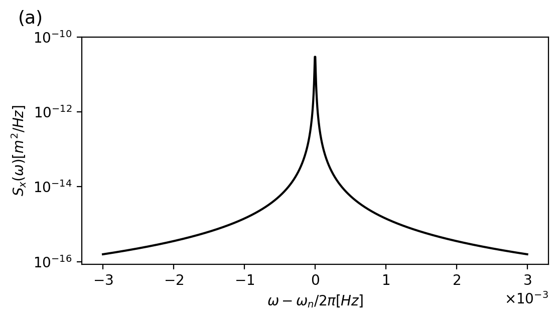
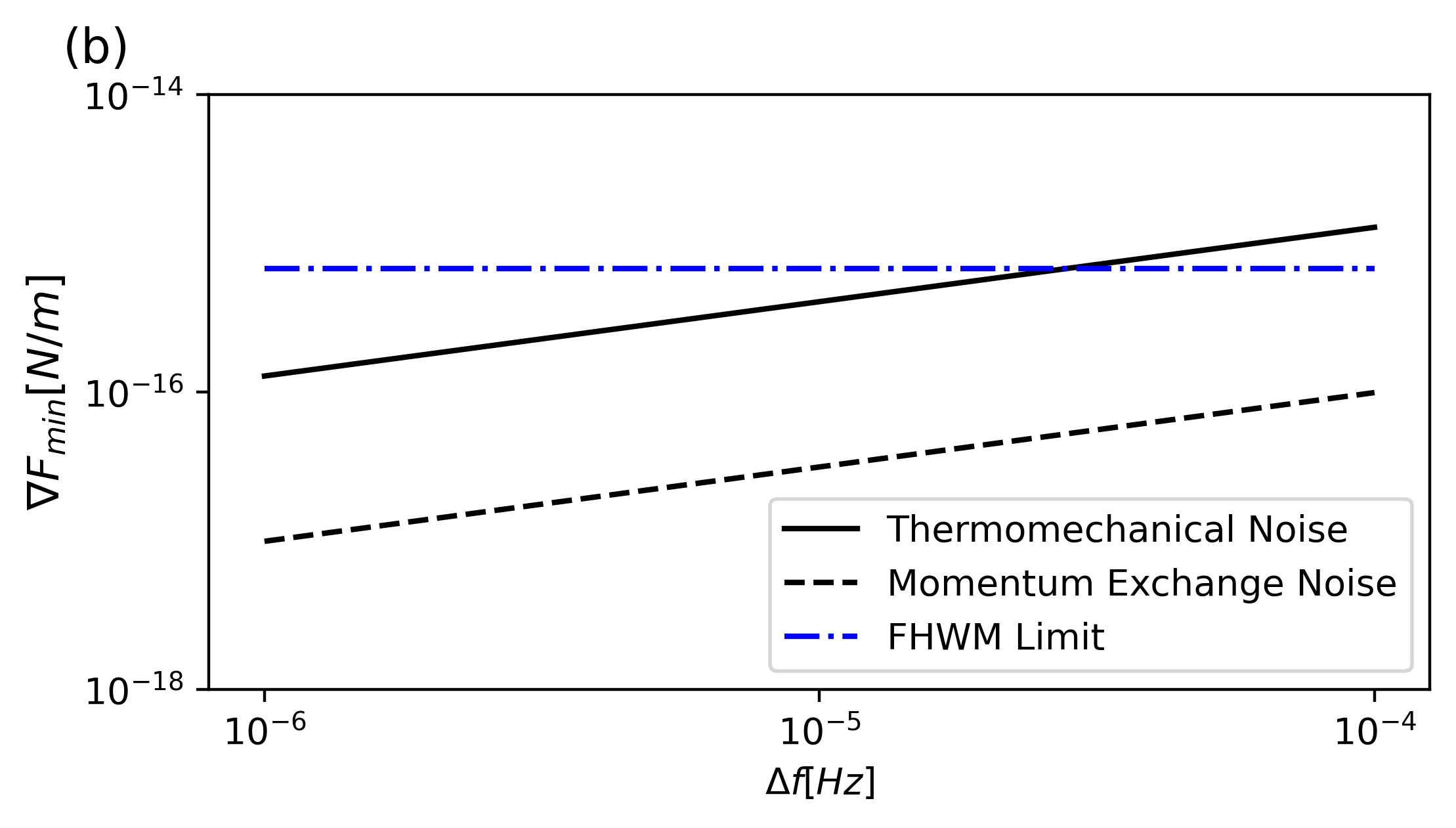
Figure 4: (a) The power spectral density of thermomechanical fluctuations as the function of the detuning to resonator frequency $\omega_{n}$. (b) Sensitivity limits due to thermomechanical fluctuations and momentum exchange noise compared to the detection limit from FWHM. The elimination of the momentum exchange noise is considered under the condition $p=10^{-10}$mbar. With the main noise limit staying below the detection result, we can ignore their influence on the system safely.

The force spectral density here is given as $S_{F}(\omega)=4m_{eff}\omega_{n}k_{B}T/Q$ with $k_{B}=1.38\times 10^{-23}$J/K as the Boltzmann’s constant and $T=293$K as the room temperature. In Fig.4, we illustrate the power spectral density of thermomechanical fluctuations to the frequency. Since $\Delta f$ is in relation to the characteristic response time $\tau=Q/2\omega$ by $\Delta f\approx 1/2\pi\tau$, we can make an estimate that the maximum measurable bandwidth $\Delta f\approx 10^{-5}$Hz. The limited minimum frequency shift can be calculated by integrating the spectral density of the frequency fluctuations $S_{\omega}(\omega)=(\omega_{n}/2Q)^{2}\cdot(S_{x}(\omega)/\langle x^{2}_{\text{rms}}\rangle)$ through the area in $\omega_{n}\pm\pi\Delta f$[63, 64]. Finally, we get

$$\Delta\omega_{n}\approx\sqrt{\frac{k_{B}T\Delta f}{m_{eff}\omega_{n}\langle x_{\text{rms}}\rangle^{2}Q}},$$ (3.5)

here $\langle x_{\text{rms}}\rangle=\sqrt{k_{B}T/m_{eff}\omega_{n}^{2}}$ represents the root-mean-square (rms) amplitude of a trapped nanosphere at thermal equilibrium.

Besides the thermomechanical noise, the momentum exchange noise from the interaction between gas molecules and resonator is another attractive noise source. According to the discussion in ref. [62], we derive the spectral density $S_{x}(\omega)$ here with a similar form to the case of thermomechanical noise

$$S_{x}(\omega)=\frac{S_{F}(\omega)}{m_{eff}^{2}((\omega^{2}-\omega_{n}^{2})^{2}+\omega^{2}\omega_{n}^{2}/Q_{gas}^{2})}.$$ (3.6)

The quality factor considering gas dissipation is defined as $Q_{gas}=m_{eff}\omega_{n}v/pA$, with $v=\sqrt{k_{B}T/m}$ is the thermal velocity of the gas molecules, $p$ the gas pressure, and $A=4\pi R^{2}$ the surface area of the nanosphere. $\Delta\omega$ can be calculated in the same way to Eq. (3.5). And it can be found in the equation that $\Delta\omega$ is proportional to the pressure $p$, indicating we can obtain higher sensitivity at higher vacuum level.

According to Eqs. (2.4) and (3.5), we have the expression of $\nabla F$ in this section as follows

$$\nabla F=\sqrt{\frac{4k_{B}T\omega_{n}m_{eff}\Delta f}{\langle x_{rms}\rangle^{2}Q}}.$$ (3.7)

To be specific, we plot $\nabla F$ as a function $\Delta f$ in the Fig. 4, showing the limit of different source of noise. Note that the limit of the dominant thermomechanical noise$\nabla F\sim 10^{-16}$N/m is lower than that of the FWHM calculation, allowing us to ignore the impact of this part of noise on the system. As for the exchange momentum noise, it is expected to be much lower in high-vacuum operation, resulting in an insignificant source of noise.

3.2 Constraints on symmetron fields

Ideally, one can place constraints on the parameters of the symmetron force with the results in Sec. 3.1 and Eq. (2.30). Before further discussing the symmetron force constraints, it is essential to consider the window of feasible $\mu$ value given by the dimension of the sphere-plate system. The upper bound of $\mu$ is related to the length of the cavity L along the resonant direction, considering the fact that only when $\mu\geq L^{-1}$ can the symmetron field have non-vanishing value in the cavity[65, 35]. For the lower bound of $\mu$, it should meet the condition that $\mu R\ll 1$[29], otherwise the reaction of the sphere on the plate-induced symmetron field will be non-negligible. Recall the system we use in Fig. 1, the radius of the sphere is $R_{sphere}$=100nm and the dimension of vacuum chamber is L=2mm. Consequently, we can only set constraints of other parameters of the symmetron force within the regime $10^{-1}$eV $\sim 10^{-4}$eV.

With the definite range values of $\mu$, we can establish the constraints on the self-coupling constant M and $\lambda$ for the next step. Firstly, we turn to the relation of parameter M and $\mu$, considering the limit of background matter density. To ensure the calculation in Sec. 2.2 remain valid, the critical density $\rho_{crit}=\mu^{2}M^{2}$ should satisfy:

$$\rho_{vac}<\mu^{2}M^{2}<\rho_{sphere}.$$ (3.8)

In the condition of this paper, the bounds are $\rho_{vac}\approx 10$eV and $\rho_{sphere}\approx 10^{18}$eV in natural units, corresponding to the density of air under $10^{-10}$mbar at room temperature and the density of fused silica.

Additionally, to meet the condition that the sphere and the plate are strongly screened, $\lambda_{sphere}\ll 1$ is required. According to the form $\lambda_{sphere}=3M^{2}/\rho R^{2}$ from Eq. (2.27), the constraint is written as

$$\frac{3M^{2}}{\rho_{sphere}R^{2}}<1.$$ (3.9)

Figure 5: Constraints of $M$ and $\mu$ derived from Eqs. (3.8) and (3.9).The horizontal line refers to the requirement that the sphere is strongly screened from Eq. (2.27).The slanted lines align with the condition that the symmetron field have non-zero value only in the vacuum cavity considering Eq. (2.22). Otherwise the spontaneous symmetry breaking will occur inside the matter, or the field will stay zero for whole system, rendering the calculation to be irrelevant.

With Eqs. (3.8) and (3.9), we illustrate the constraints in Fig. 5. The horizontal line corresponds to the result in Eq. (3.9), while the other two lines refer to the limits on M imposed through Eq. (3.8).And the center area filled with dark blue is the constraint we obtain.

The final step toward a complete constraint of symmetron force is to determine the range of $\lambda$. The forecast constraint on $\lambda$ is connected to our optomechanical detection by Eq. (2.30). Notice that a higher force gradient $\nabla F$ indicate a smaller value of $\lambda$ for fixed $\mu$ and M. Thus, one can rule out the values of $\lambda$ which lead to a higher $\nabla F$ than the limit obtained in Eq. (3.3). Besides, $\lambda>0$ is necessary to make the symmetron mechanism to work.

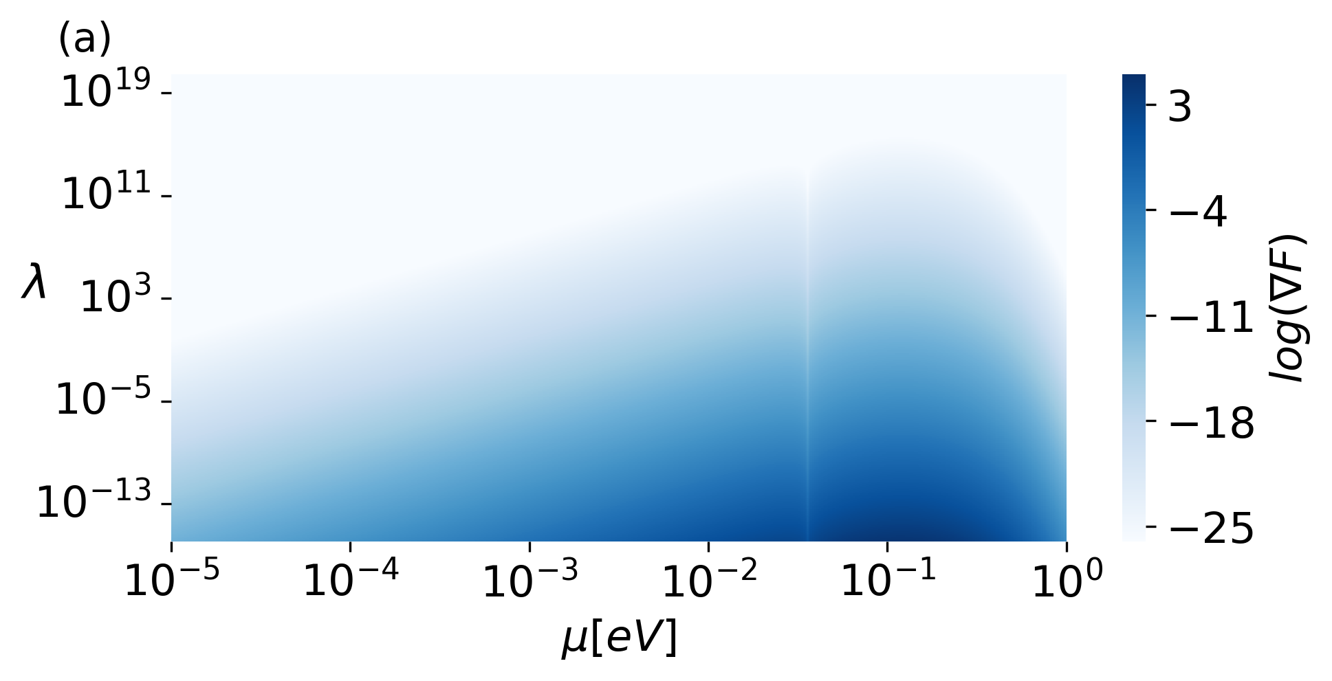
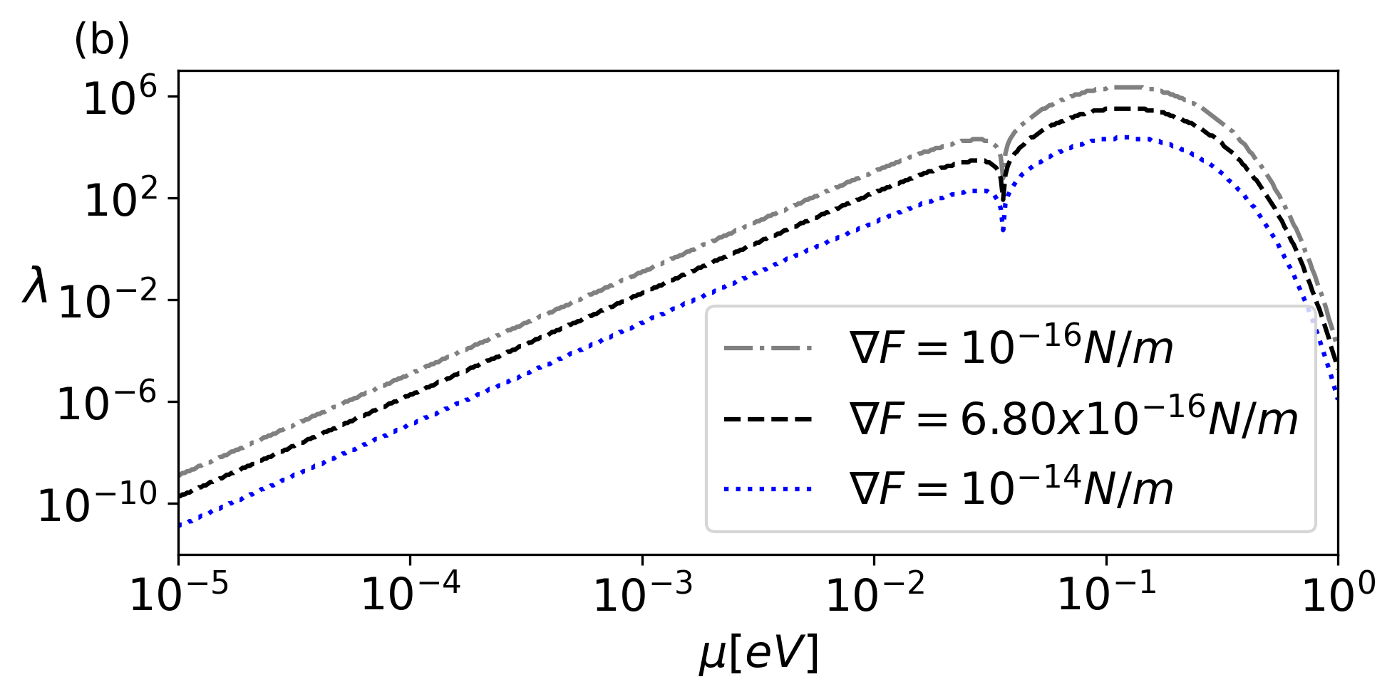
Figure 6: (a) Symmetron-induced force gradient as the function of $\mu$ and $\lambda$, with the detect sphere of R=100nm located at d=5$\mu$m from the surface of source mass. (b) Forecast constraints on symmetron parameters $\mu$ and $\lambda$ according to the minimum $\nabla F$ in Sec. 3.1. The three curves correspond to three bounds given by different sensitivities of $\nabla F=10^{-16}N/m,6.80\times 10^{-16}N/m,10^{-14}N/m$ from the top to the bottom. Recall that the value of $\lambda$ which indicates larger $\nabla F$ than the result in Eq. (3.3) will be ruled out. Namely, the area under the bound given by the black dashed line will be excluded.

In Fig. 6, we illustrate the value of force gradient $\nabla F$ with different values of M and $\mu$. Considering the data points obtained, a curve indicating the result achieved with optomechanical detection is plotted in Fig. 6. The value of $\lambda$ under the curve will be ruled out. It should be emphasized that the parameter discussed are constrainable only in range $10^{-1}$eV $\sim 10^{-4}$eV. Consequently, we can finally establish a comprehensive area of parameters to exclude with the discussion in Sec. 3.2.

In Fig. 7, we plot the constraints with discrete value of $\mu$. Our work is highlighted in dark blue while other constraints are filled with light blue, including an unperformed Casimir-force design[29], atom interferometry[66], torsion balance[35], and ultracold bouncing neutron experiments[38]. Our hypothetical scheme is particularly effective for high value of $\mu$, which is found to exclude larger area compared to other methods. One can see that torsion balance method provides extra bounds in $M>10$Gev regime and atom interferometry gives strong constraints for $\mu=10^{-4}$eV, which are largely complementary to the force-based detection results such as this work and the Casimir-force experiment. Additionally, the area $M\sim 1$Gev is well constrained by the bouncing neutrons experiment, which has the potential to expand its constraint up to $\mu\sim$eV. Similar to our method, the Casimir-force constraints are provided through the minimum different force $\delta F$ of the symmetron field in a vacuum chamber at two locations[67]. This method shows a good ability to cover an extended range of $\sim$ 7 orders of magnitude. Taking all the constraints together into account, we can find that a substantial area in parameter space has been excluded.

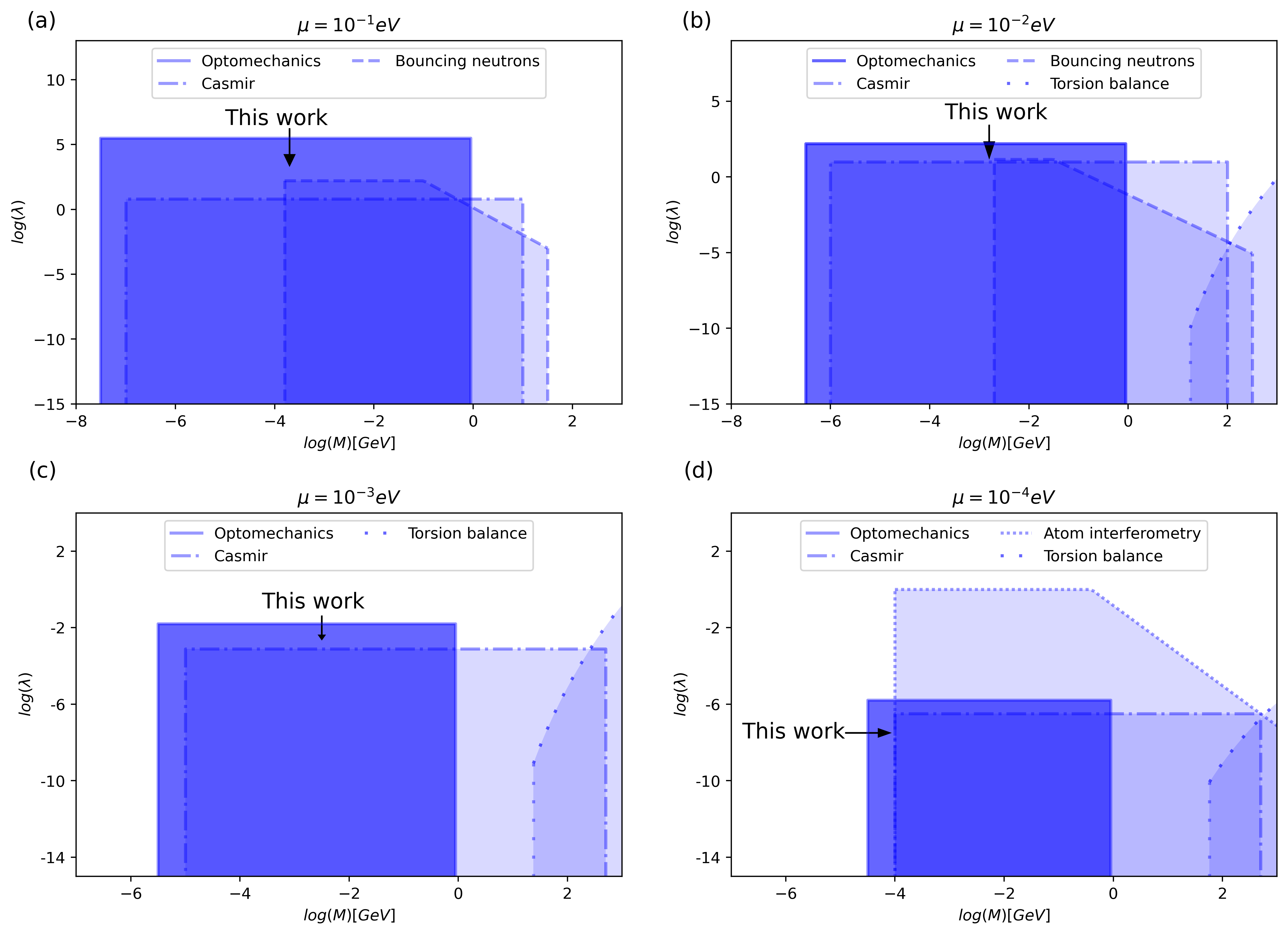
Figure 7: Symmetron constraints from our hypothetical experiment scheme with other bounds in Casimir-force design, atom interferometry, torsion balance, and ultracold bouncing neutron measurements reproduced from refs. [29, 66, 35, 38] respectively. The excluded area of our method is based on the result in Figs. 5 and 6 in range of $10^{-1}$eV $\sim 10^{-4}$eV, and shown within four discrete values $\mu=10^{-1}eV,10^{-2}eV,10^{-3}eV,10^{-4}eV$.

4 Conclusion

In this paper, an optomechanical method is developed to set constraints on the symmetron force. In a system consisting a dense but small sphere and a relatively large plate, we demonstrate the behavior of the symmetron field with the screening mechanism. Via the theory of quantum optics, we derive the solution of the transmission spectrum and the function of associated noise in detection process. Further, the relation between symmetron-force-induced frequency shift and the optical measurable parameters is established, which leads to the minimum detectable force gradient. Based on results of the hypothetical experiment in our scheme, we deduce constraints on the symmetron force parameters, which make significant progress particularly for $\mu=0.1$eV of 3 orders of magnitude. Besides, there is still some work to do for future experiments and numerical simulation. With high-finesse cavities with larger volume and the method of cavity-assisted cooling [68, 69, 70, 71], hyperfine spectrum and more sensitive detection can be achieved. More precise numerical relaxation techniques can be introduced in force calculations, which can be found in refs[41, 72]. And approximations for complex geometries could be helpful for more reliable constraints[73, 74]. With the progress of experimental technology, we believe that there will be more actual optomechanics-based detection devices in the near future.

References

- [1] P. Brax, What makes the universe accelerate? a review on what dark energy could be and how to test it, Reports on Progress in Physics 81 (2017) 016902.
- [2] A.G. Riess, A.V. Filippenko, P. Challis et al., Observational evidence from supernovae for an accelerating universe and a cosmological constant, The Astronomical Journal 116 (1998) 1009.
- [3] B.P. Schmidt, N.B. Suntzeff, M.M. Phillips et al., The high-z supernova search: Measuring cosmic deceleration and global curvature of the universe using type ia supernovae, The Astrophysical Journal 507 (1998) 46.
- [4] H. Desmond, B. Jain and J. Sakstein, Local resolution of the hubble tension: The impact of screened fifth forces on the cosmic distance ladder, Phys. Rev. D 100 (2019) 043537.
- [5] L. Lombriser, On the cosmological constant problem, Physics Letters B 797 (2019) 134804.
- [6] H.E.S. Velten, R.F. vom Marttens and W. Zimdahl, Aspects of the cosmological “coincidence problem”, The European Physical Journal C 74 (2014) .
- [7] J. Solà, Cosmological constant and vacuum energy: old and new ideas, Journal of Physics: Conference Series 453 (2013) 012015.
- [8] Planck Collaboration, Aghanim, N., Akrami, Y. et al., Planck 2018 results - vi. cosmological parameters (corrigendum), A & A 652 (2021) C4.
- [9] A.G. Riess, W. Yuan, L.M. Macri et al., A comprehensive measurement of the local value of the hubble constant with 1 km/s·mpc uncertainty from the hubble space telescope and the sh0es team, The Astrophysical Journal Letters 934 (2022) L7.
- [10] Böhringer, Hans, Chon, Gayoung and Collins, Chris A., Observational evidence for a local underdensity in the universe and its effect on the measurement of the hubble constant, A& A 633 (2020) A19.
- [11] J.H.W. Wong, T. Shanks, N. Metcalfe and J.R. Whitbourn, The local hole: a galaxy underdensity covering 90 percent of sky to 200Mpc, Monthly Notices of the Royal Astronomical Society 511 (2022) 5742.
- [12] N. Schöneberg, G.F. Abellán, A.P. Sánchez et al., The H0 olympics: A fair ranking of proposed models, Physics Reports 984 (2022) 1.
- [13] M.S. Safronova, D. Budker, D. DeMille et al., Search for new physics with atoms and molecules, Rev. Mod. Phys. 90 (2018) 025008.
- [14] S.M. Feeney, D.J. Mortlock and N. Dalmasso, Clarifying the Hubble constant tension with a Bayesian hierarchical model of the local distance ladder, Monthly Notices of the Royal Astronomical Society 476 (2018) 3861.
- [15] W. Cardona, M. Kunz and V. Pettorino, Determining h0 with bayesian hyper-parameters, Journal of Cosmology and Astroparticle Physics 2017 (2017) 056.
- [16] D. Camarena, V. Marra, Z. Sakr et al., The Copernican principle in light of the latest cosmological data, Monthly Notices of the Royal Astronomical Society 509 (2021) 1291.
- [17] E.J. COPELAND, M. SAMI and S. TSUJIKAWA, Dynamics of dark energy, International Journal of Modern Physics D 15 (2006) 1753.
- [18] M. Högås and E. Mörtsell, Hubble tension and fifth forces, Phys. Rev. D 108 (2023) 124050.
- [19] A. Joyce, B. Jain, J. Khoury and M. Trodden, Beyond the cosmological standard model, Physics Reports 568 (2015) 1.
- [20] C. Burrage, E.J. Copeland and E. Hinds, Probing dark energy with atom interferometry, Journal of Cosmology and Astroparticle Physics 2015 (2015) 042.
- [21] S. Qvarfort, D. Rätzel and S. Stopyra, Constraining modified gravity with quantum optomechanics, New Journal of Physics 24 (2022) 033009.
- [22] P. Brax, A.-C. Davis, B. Li et al., Unified description of screened modified gravity, Phys. Rev. D 86 (2012) 044015.
- [23] K. Hinterbichler, J. Khoury, A. Levy et al., Symmetron cosmology, Phys. Rev. D 84 (2011) 103521.
- [24] P. Brax and P. Valageas, -mouflage cosmology: The background evolution, Phys. Rev. D 90 (2014) 023507.
- [25] A. Vainshtein, To the problem of nonvanishing gravitation mass, Physics Letters B 39 (1972) 393.
- [26] L. Ogden, K. Brown, H. Mathur and K. Rovelli, Electrostatic analogy for symmetron gravity, Phys. Rev. D 96 (2017) 124029.
- [27] E. Babichev, C. Deffayet and R. Ziour, k-MOUFLAGE Gravity, International Journal of Modern Physics D 18 (2009) 2147.
- [28] A. Nicolis, R. Rattazzi and E. Trincherini, Galileon as a local modification of gravity, Phys. Rev. D 79 (2009) 064036.
- [29] B. Elder, V. Vardanyan, Y. Akrami et al., Classical symmetron force in casimir experiments, Phys. Rev. D 101 (2020) 064065.
- [30] C. Burrage, A. Kuribayashi-Coleman, J. Stevenson et al., Constraining symmetron fields with atom interferometry, Journal of Cosmology and Astroparticle Physics 2016 (2016) 041.
- [31] P. Brax, Screening mechanisms in modified gravity, Classical and Quantum Gravity 30 (2013) 214005.
- [32] M. Pietroni, Dark energy condensation, Phys. Rev. D 72 (2005) 043535.
- [33] The Euclid Theory Working Group, L. Amendola, S. Appleby, A. Avgoustidis, D. Bacon, T. Baker et al., Cosmology and fundamental physics with the euclid satellite, Living Reviews in Relativity 21 (2018) .
- [34] D.J. Kapner, T.S. Cook, E.G. Adelberger et al., Tests of the gravitational inverse-square law below the dark-energy length scale, Phys. Rev. Lett. 98 (2007) 021101.
- [35] A. Upadhye, Symmetron dark energy in laboratory experiments, Phys. Rev. Lett. 110 (2013) 031301.
- [36] R.S. Decca, D. López, E. Fischbach et al., Tests of new physics from precise measurements of the casimir pressure between two gold-coated plates, Phys. Rev. D 75 (2007) 077101.
- [37] S.K. Lamoreaux, Demonstration of the casimir force in the 0.6 to range, Phys. Rev. Lett. 78 (1997) 5.
- [38] G. Cronenberg, P. Brax, H. Filter et al., Acoustic rabi oscillations between gravitational quantum states and impact on symmetron dark energy, Nature Physics 14 (2018) .
- [39] H. Fischer, C. Käding, H. Lemmel et al., Search for dark energy with neutron interferometry, Progress of Theoretical and Experimental Physics 2024 (2024) .
- [40] P. Brax and A.-C. Davis, Atomic interferometry test of dark energy, Phys. Rev. D 94 (2016) 104069.
- [41] M. Jaffe, P. Haslinger, V. Xu et al., Testing sub-gravitational forces on atoms from a miniature, in-vacuum source mass, Nature Physics 13 (2016) .
- [42] L. Chen, J. Liu and K.-D. Zhu, Constraining the axion-nucleon coupling and non-newtonian gravity with a levitated optomechanical device, Phys. Rev. D 106 (2022) 095007.
- [43] A.A. Geraci, S.B. Papp and J. Kitching, Short-range force detection using optically cooled levitated microspheres, Phys. Rev. Lett. 105 (2010) 101101.
- [44] J. Liu and K.-D. Zhu, Nanogravity gradiometer based on a sharp optical nonlinearity in a levitated particle optomechanical system, Phys. Rev. D 95 (2017) 044014.
- [45] C. Genes, D. Vitali, P. Tombesi et al., Ground-state cooling of a micromechanical oscillator: Comparing cold damping and cavity-assisted cooling schemes, Phys. Rev. A 77 (2008) 033804.
- [46] V. Giovannetti and D. Vitali, Phase-noise measurement in a cavity with a movable mirror undergoing quantum brownian motion, Phys. Rev. A 63 (2001) 023812.
- [47] C. Gardiner and P. Zoller, Quantum Noise: A Handbook of Markovian and Non-Markovian Quantum Stochastic Methods with Applications to Quantum Optics, Springer Series in Synergetics, Springer (2004).
- [48] R. Boyd and D. Prato, Nonlinear Optics, Elsevier Science (2008).
- [49] W. Bowen and G. Milburn, Quantum Optomechanics, CRC Press (2015).
- [50] P. Brax and M. Pitschmann, Exact solutions to nonlinear symmetron theory: One- and two-mirror systems, Phys. Rev. D 97 (2018) 064015.
- [51] C. Burrage, B. Elder and P. Millington, Particle level screening of scalar forces in dimensions, Phys. Rev. D 99 (2019) 024045.
- [52] L. Hui, A. Nicolis and C.W. Stubbs, Equivalence principle implications of modified gravity models, Phys. Rev. D 80 (2009) 104002.
- [53] K. Hinterbichler and J. Khoury, Screening long-range forces through local symmetry restoration, Phys. Rev. Lett. 104 (2010) 231301.
- [54] U. Delić, D. Grass, M. Reisenbauer et al., Levitated cavity optomechanics in high vacuum, Quantum Science and Technology 5 (2020) 025006.
- [55] Z. Jiang, Z. Wu, W. Yang et al., Numerical simulations on narrow-linewidth photonic microwave generation based on a qd laser simultaneously subject to optical injection and optical feedback, Appl. Opt. 59 (2020) 2935.
- [56] J. Gieseler, L. Novotny and R. Quidant, Thermal nonlinearities in a nanomechanical oscillator, Nature Physics (2013) .
- [57] S. Groeblacher, K. Hammerer, M. Vanner et al., Observation of strong coupling between a micromechanical resonator and an optical cavity field, Nature 460 (2009) 724.
- [58] D. Hunger, T. Steinmetz, Y. Colombe et al., A fiber fabry–perot cavity with high finesse, New Journal of Physics 12 (2010) 065038.
- [59] D.E. Chang, C.A. Regal, S.B. Papp et al., Cavity opto-mechanics using an optically levitated nanosphere, Proceedings of the National Academy of Sciences 107 (2010) 1005.
- [60] P. Berman and V. Malinovsky, Principles of Laser Spectroscopy and Quantum Optics, Princeton University Press (2011).
- [61] H. Mori, Statistical-Mechanical Theory of Kinetic Equations: Kinetic Equations for Dense Gases and Liquids, Progress of Theoretical Physics 49 (1973) 1516.
- [62] K.L. Ekinci, Y.T. Yang and M.L. Roukes, Ultimate limits to inertial mass sensing based upon nanoelectromechanical systems, Journal of Applied Physics 95 (2004) 2682.
- [63] A.N. Cleland and M.L. Roukes, Noise processes in nanomechanical resonators, Journal of Applied Physics 92 (2002) 2758.
- [64] W. Robins and I. of Electrical Engineers, Phase Noise in Signal Sources: Theory and Applications, IEE telecommunications series, P. Peregrinus (1984).
- [65] P. Brax and A.-C. Davis, Casimir, gravitational, and neutron tests of dark energy, Phys. Rev. D 91 (2015) 063503.
- [66] D.O. Sabulsky, I. Dutta, E.A. Hinds et al., Experiment to detect dark energy forces using atom interferometry, Phys. Rev. Lett. 123 (2019) 061102.
- [67] Y.-J. Chen, W.K. Tham, D.E. Krause et al., Stronger limits on hypothetical yukawa interactions in the 30–8000 nm range, Phys. Rev. Lett. 116 (2016) 221102.
- [68] Y.-C. Liu, R.-S. Liu, C.-H. Dong et al., Cooling mechanical resonators to the quantum ground state from room temperature, Phys. Rev. A 91 (2015) 013824.
- [69] M. Hosseini, Y. Duan, K.M. Beck et al., Cavity cooling of many atoms, Phys. Rev. Lett. 118 (2017) 183601.
- [70] Particle Data Group collaboration, Review of particle physics, Phys. Rev. D 98 (2018) 030001.
- [71] C.J. Hood, H.J. Kimble and J. Ye, Characterization of high-finesse mirrors: Loss, phase shifts, and mode structure in an optical cavity, Phys. Rev. A 64 (2001) 033804.
- [72] B. Elder, J. Khoury, P. Haslinger et al., Chameleon dark energy and atom interferometry, Phys. Rev. D 94 (2016) 044051.
- [73] P. Brax, C. van de Bruck, A.-C. Davis et al., Detecting chameleons through casimir force measurements, Phys. Rev. D 76 (2007) 124034.
- [74] D.E. Krause, R.S. Decca, D. López et al., Experimental investigation of the casimir force beyond the proximity-force approximation, Phys. Rev. Lett. 98 (2007) 050403.