Analytic Continuation by Feature Learning
Abstract
Analytic continuation aims to reconstruct real-time spectral functions from imaginary-time Green’s functions; however, this process is notoriously ill-posed and challenging to solve. We propose a novel neural network architecture, named the Feature Learning Network (FL-net), to enhance the prediction accuracy of spectral functions, achieving an improvement of at least over traditional methods, such as the Maximum Entropy Method (MEM), and previous neural network approaches. Furthermore, we develop an analytical method to evaluate the robustness of the proposed network. Using this method, we demonstrate that increasing the hidden dimensionality of FL-net, while leading to lower loss, results in decreased robustness. Overall, our model provides valuable insights into effectively addressing the complex challenges associated with analytic continuation.
I Introduction
Imaginary-time Green’s functions, which can be directly obtained from quantum Monte Carlo simulations, are fundamental in characterizing many-body systemsGull et al. (2010); Georges et al. (1996). However, to understand the real-time dynamics and corresponding spectral functions, analytic continuation is required to extract spectral densities and real-time responses from these imaginary-time dataJarrell and Gubernatis (1996); Schollwoeck (2010).
Mathematically, analytic continuation involves solving a Fredholm integral equation of the first kind to reconstruct the spectral density on the real axis from the Green’s function defined on the imaginary axisJarrell and Gubernatis (1996); Gubernatis et al. (1991). The relationship between these quantities can be expressed by the following integral equationMahan (2000); Kabanikhin (2011):
| (1) |
where is the Green’s function at Matsubara frequency , and is the spectral density to be determined. The ill-conditioned kernel makes the inverse problem highly sensitive to small errors in the input data, which leads to significant variations in the resulting spectral density. Due to this sensitivity, analytic continuation is classified as an ill-posed problem, with solutions that are often non-unique and susceptible to noise. Willoughby (1979). The key challenge is to obtain stable and reliable solutions. Bryan (1990).
Several approaches have been developed to address this challenge. NevanlinnaFei et al. (2021) and Padé approximationsKiss (2019); Vidberg and Serene (1977); Weh et al. (2020) provide efficient rational function approximations, while methods like singular value decomposition (SVD)Gunnarsson et al. (2010) and Tikhonov regularizationHansen (1992); Ghanem and Koch (2023a) mitigate noise but increase computational complexity. The maximum entropy method (MEM)Skilling (1989); Bergeron and Tremblay (2016); Ghanem and Koch (2023b); Rumetshofer et al. (2019); Reymbaut et al. (2015) is popular for smoothing noisy data but struggles with resolving sharp peaks and coherent excitationsFournier et al. (2020).
Recently, neural networks have been explored as a promising method for mapping imaginary-time Green’s functions to real-time spectral functions. By directly learning a mapping from to using a given dataset, neural networks can outperform traditional methods such as MEMFournier et al. (2020); Yao et al. (2022); Huang and Yang (2022); Hendry and Feiguin (2019). However, the trained networks often perform poorly when dealing with multi-peak or sharp-peak spectra and struggle under significant noiseRakin et al. (2019). Moreover, previous studies have lacked comprehensive analyses of the robustness of these networks, which limits their broader adoption.
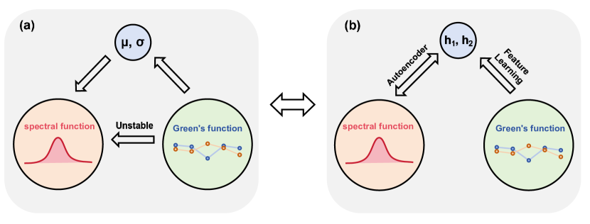
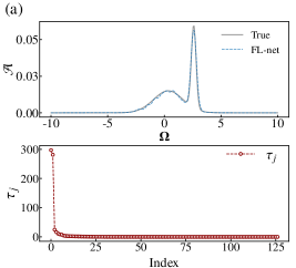
In this paper, we propose a new network architecture that significantly improves the accuracy of spectral function prediction and provides a thorough analysis of its robustness. Our new architecture is founded on a simple observation: the spectral function can always be captured by a few features such as the width, the weight or the position of the peaks. In this sense, although or is a high dimensional vector, they can be parameterized by a few features for specific kind of systems. As an instance shown in Fig. 1(a), in single-peak Gaussian spectra, both and are uniquely determined by the mean and the variance of the Gaussian. Hence, though direct mapping from to is sensitive to the noise in , another pass from to to can be more stable. For general data set without any prior knowledge about the features of the spectrum, as shown in Fig. 1(b), similar strategy can be applied by first learning the underlying feature of the data set by an auto-encoder and then training a network that map to those features.
The rest of this paper is organized as follows. In Section II, we introduce the design principles of the proposed network architecture and describe the training process, highlighting how the spectral function’s key characteristics are leveraged to construct an effective model. In Section III, we examine the impact of hidden feature dimensionality on model performance through experimental studies and evaluate the effectiveness of different approaches across various datasets. In Section IV, we propose a method utilizing singular value decomposition (SVD) to analyze the robustness of FL-net and compare its robustness across different hidden dimensionalities. Finally, in Section V, we summarize our findings and propose potential directions for future research.
II Network structure
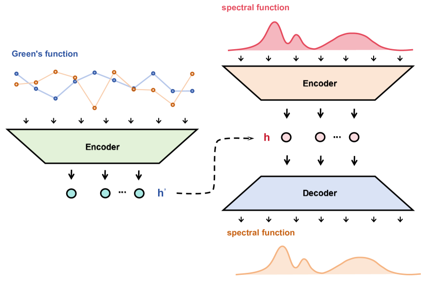
We propose the Feature Learning Network (FL-net), as illustrated in Fig. 2, based on the described methodology. To prepare and as input and output for the neural network, we discretize into a dimensional vector and implement a cutoff on the order of Matsubara frequency for . To be clear, each input data of the spectral function is a vector in the formApp :
| (2) |
The Matsubara Green’s function is considered, which is defined at Matsubara frequencies for , where is the inverse temperature, with and denoting Boltzmann’s constant and temperature, respectively. At each Matsubara frequency, can be decomposed into its real and imaginary parts: . The vector is formed by arranging these components sequentially:
| (3) | ||||
The training process consisting of three main steps:
First, the auto-encoder consists of two mappings: the encoder and the decoder , where both and are discrete approximations of the ideal mappings. The latent vector
| (4) |
with adjustable dimension , represents the statistical features extracted from . We consider a dataset containing samples, indexed by . The loss function used to train the auto-encoder is:
| (5) |
where and denote the true and predicted spectral functions for the -th sample, respectively, and represents the norm.
Next, we train an encoder performs the approximate mapping , where is an approximation of the latent feature . The loss function used for training is:
| (6) |
Finally, we retrain the mapping , completing the transformation App . By targeting the latent feature space , FL-net incorporates prior knowledge of the spectral function’s peak structures and characteristic distributions.
The network is optimized using the Adam optimizer Kingma and Ba (2014). To balance the influence of each dataset and render the loss dimensionless, we normalize the mean squared error (MSE) by the average variance of the true values. The normalized loss function is defined as:
| (7) |
where , and represents the variance of the true values of the -th component across the dataset. This normalization mitigates the effect of varying data scales, allowing consistent evaluation across datasets. We use the normalized loss function for all subsequent model evaluations to ensure fair comparisons across datasets.
The code is available for reproduction and further exploration.111GitHub repository: https://github.com/Order-inz/Analytic-Continuation-by-Feature-Learning.
III Hidden Feature and Model Performance
We evaluate the performance of FL-net on a dataset of synthetic spectral functions, each generated as a summation of Gaussian distributions:
| (8) |
where each peak is characterized by a mean , a standard deviation , and . The parameters and are uniformly generated within their respective ranges. The weight coefficients satisfy the normalization condition: . Using this method, we generate 100,000 spectral functions. The corresponding Green’s functions are obtained from the linear mapping described in Eq. (1).
We first consider a simple dataset which is consist of single peak Gaussian (). By setting the hidden dimension of FL-net to 2, we obtain a considerably small prediction loss on the test set as . Interestingly, when we use the prior knowledge of Gaussian spectral by setting network mapping process as App , the prediction loss instead increased to , suggesting that the FL-net has found a more suitable expression for the hidden variable. However, in this single peak Gaussian case, we find the hidden variable compressed by FL-net is actually equivalent to by numerically computing the Jacobian matrix :
| (9) |
As an example, the Jacobian matrix evaluated at and is given by: , which is a full rank matrix, indicating that the hidden features are locally equivalent to and .
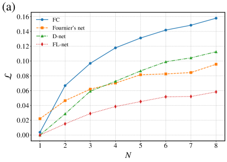
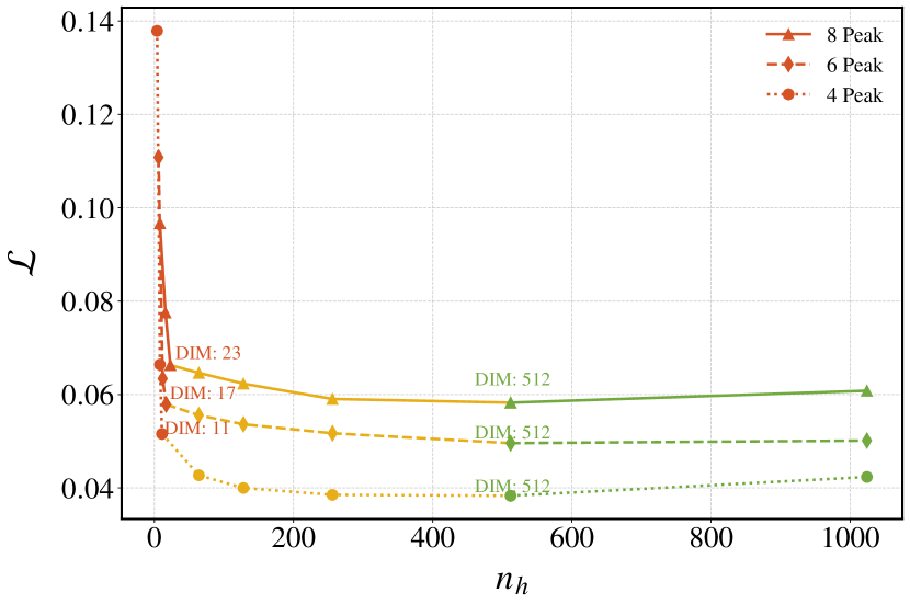
For a more general dataset with multi-peak spectra, we begin by investigating how the dimension of the hidden variable affects the performance of FL-net. As shown in Fig.3, increasing leads to a rapid decrease in of test data until approaches — the number of independent free parameters in our synthetic data. When exceeds , the network’s loss continues to decrease at a slower rate, yielding only marginal gains. However, further increasing beyond 512 results in an increase in the loss. This performance degradation can be attributed to data sparsity in high-dimensional spaces, which leads to model overfitting and consequently reduces its generalization ability Glorot et al. (2011). Based on these observations, we will henceforth set , striking an optimal balance between performance and computational efficiency.
To verify the effectiveness of the FL-net structure, we introduce a reference network (D-net) with a comparable number of parameters but without utilizing the feature as the intermediate layerApp . As illustrated in Fig. 4(a), we compare the performance of FL-net and D-net across datasets with varying peak numbers . This comparison clearly shows that incorporating hidden features significantly enhances the accuracy of analytic continuation. Furthermore, we also evaluated FL-net’s performance against networks from previous literatureFournier et al. (2020)(Fournier’s net) and simple fully connected networks (FC net). The results consistently demonstrated FL-net’s superiority in the task of analytic continuation.
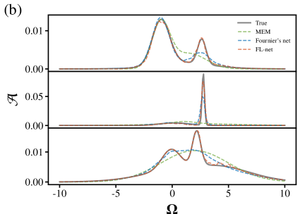
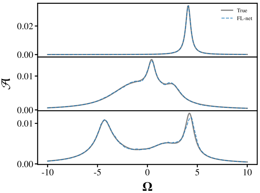
We compare the predictions of FL-net, Fournier’s net, and the Maximum Entropy Method (MEM) with the ground truth for randomly selected samples, as illustrated in Fig.4(b). In the case of double peaks, both MEM and Fournier’s net struggle to capture the characteristics of the second peak accurately. For sharp spectra, MEM tends to produce overly smooth results, failing to capture prominent features. As spectral complexity increases, such as in multi-peak scenarios, neither MEM nor Fournier’s net adequately captures the complex details. In contrast, FL-net consistently reproduces results closely matching the true spectra, demonstrating superior accuracy in handling complex spectral structures. The strong generalization ability of FL-net on Gaussian datasets suggests its potential for broader applications, including Lorentzian spectra App .
IV Robustness Analysis
To examine the robustness of the trained FL-net, we consider the relationship between a small perturbation in the input imaginary-time Green’s function and the corresponding change in the output spectral function , which can be expressed as:
| (10) |
where the matrix can be naturally obtained from the gradient of the trained neural network. The structure of can be further analyzed by the singular value decomposition (SVD) :
| (11) |
where and are orthogonal matrices. The matrix is an orthogonal matrix:
| (12) |
where each is a column vector given by:
| (13) |
Here, represents the -th eigenmode of in response to noise in . In addition, contains the right singular vectors . The diagonal matrix contains the singular values , which quantify the magnitude of ’s response to perturbations in . We assume the noise is totally random, hence the property of the response is determined by and .
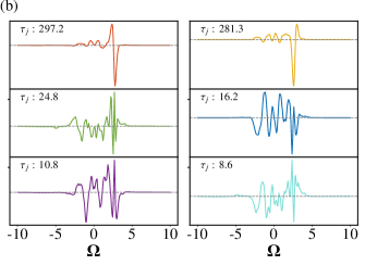
The distribution of for a fixed is shown in Fig.5(a), it appears that there are two modes with significantly larger strength than the remaining ones. However, by further analyzing the pattern of for large , as illustrated in Fig.5(b), we find their amplitudes are mainly concentrated at the peak locations of the original spectrum . In fact, the significant overlap between and distributions implies that perturbations in the direction only cause small disturbance to . The magnitude of this disturbance is given by the following equationApp :
| (14) |
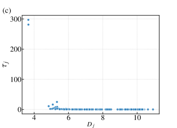
which is the logarithm of the Fisher information along direction. In Fig 5(c), we plot the singular values of each mode against their corresponding . It is observed that the two modes with the largest are captured by the smallest , while the rest modes with small have very large . Notice that represents the overall amplification of the corresponding mode . Therefore, the noise sensitivity of each mode should be
| (15) |
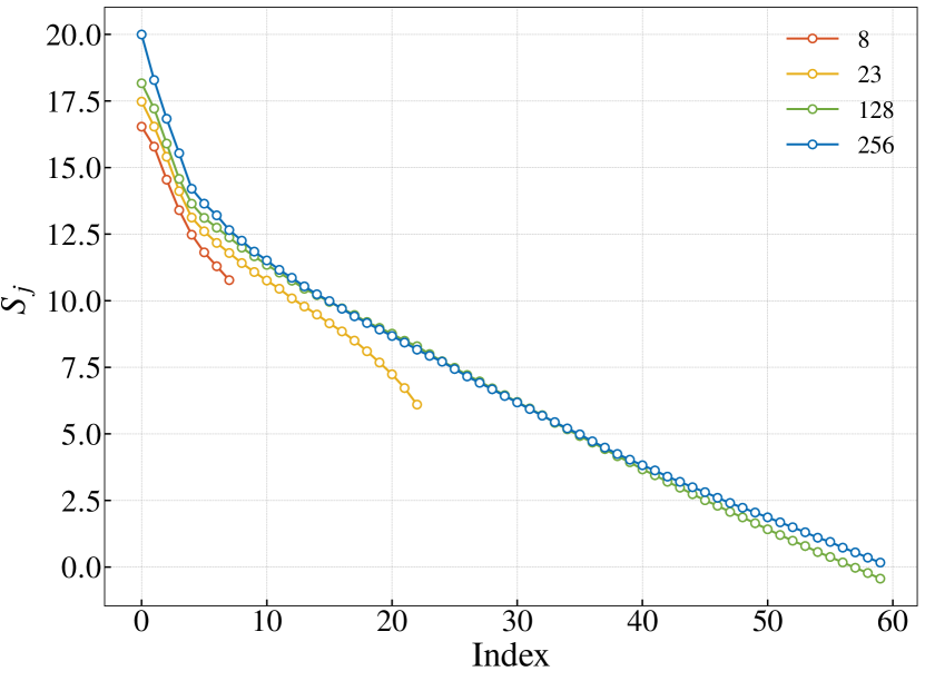
To generally evaluate the robustness of FL-net under different hidden feature dimensions , we conducted experiments based on a 1-to-8 peak mixed sample dataset and averaged the values across the dataset. As shown in Fig. 6, for networks with lower dimensions, we present the values corresponding to the intermediate hidden layer features; for networks with higher dimensions, we show the top 60 largest values. The analysis results indicate that as increases, decreases, whereas the sensitivity of the network to noise increases.
V Conclusions
In this study, we introduce a novel neural network architecture, the Feature Learning Network (FL-net), designed to learn key statistical properties and essential modes for reconstructing spectral functions. Our results demonstrate that FL-net significantly outperforms previous methods in terms of prediction accuracy. Furthermore, we develop an analytical method to evaluate the robustness of the network. Our analysis reveals that, although increasing the latent feature dimensionality can reduce prediction loss, it may also compromise robustness.
FL-net leverages feature learning to capture the core statistical attributes of spectral functions, providing a new approach for applying machine learning to ill-posed inverse problems. This mechanism has the potential to advance both theoretical understanding and practical applications across a variety of domains. In conclusion, FL-net not only achieves substantial improvements in tackling the analytic continuation problem but also establishes a foundation for applying similar approaches to other complex inverse problems in physics.
VI Acknowledgement
We thank Juan Yao for inspiring discussion. This work is supported by the National Natural Science Foundation of China (NSFC) under Grant Nos. 12204352 (CW).
Appendix A Maximum Entropy Method (MEM)
The classical Maximum Entropy Method is formulated within the framework of Bayesian statistics, as described by Bayes’ theorem:
| (16) |
where represents the imaginary-time Green’s function obtained through quantum Monte Carlo simulations, and is the target spectral function. By maximizing , we obtain the spectral function that best aligns with the data, while adhering to the prior information encoded in the default model.
In this context, , where quantifies the deviation between the reconstructed and measured Green’s functions, defined as:
| (17) |
where is the transformation matrix mapping the spectral function to the Green’s function , and is the covariance matrix representing the uncertainties in the data.
The prior probability is given by , where is the entropy term of the spectral function, defined as:
| (18) |
where is the default model, representing prior knowledge about the spectral function.
Thus, maximizing the objective function provides the optimal solution for the spectral function . Once the optimization process converges, the resulting spectral function can be validated against experimental data to assess its reliability.
Appendix B The details of FL-net, D-net
We discretize the training data for the FL-net by sampling the spectral function and the Green’s function as follows: For , we sample 256 evenly spaced points over the range ], forming a 256-dimensional vector:
| (19) |
For , we sample at Matsubara frequencies with , obtaining 64 sample points. We separate the complex values into real and imaginary parts and arrange them sequentially to form a 128-dimensional vector:
| (20) |
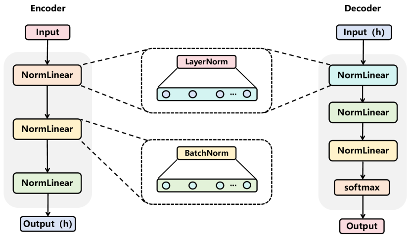
The network architecture consists of two encoders and one decoder. The encoders for and share the same structure to ensure consistent latent feature distributions (see Fig. 7). Each encoder primarily uses NormedLinear modules, which include either batch normalization or layer normalization for normalization, and linear layers for feature mapping. The decoder incorporates a softmax layer after the last encoder layer to normalize the predicted spectral function.
For the encoder of the imaginary-time Green’s function , the NormedLinear modules utilize batch normalization, which is well-suited for handling Green’s functions. In contrast, the encoder for the spectral function employs layer normalization. Layer normalization is preferred for because it efficiently manages variations across individual inputs, unlike batch normalization, which may struggle with such variability. By normalizing across layer dimensions and acting on different features within a single sample, layer normalization is more appropriate for analyzing the spectral functionVaswani et al. (2017); Jiang et al. (2021).
All layers use the Exponential Linear Unit (ELU) activation function, which maintains non-zero gradients for negative inputs, outperforming ReLU in our experimentsClevert et al. (2015).
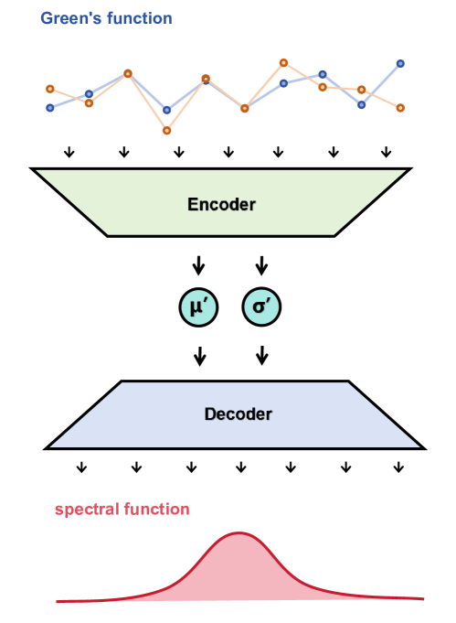
In the spectral feature learning process, the network trains the encoder by using the Green’s function to directly learn the spectral parameters and , and then uses the encoder to generate new parameters and to reconstruct the spectral function . The goal is to establish a mapping from , as illustrated in Fig. 8.
In the D-net, the encoder for is directly linked to the decoder for , establishing a direct mapping . In contrast to the FL-net, which uses an intermediate latent space to capture spectral features, the D-net bypasses this intermediate feature learning. This direct approach enables a clear comparison to assess the effectiveness of the FL-net’s feature learning structure.
Appendix C Results of Lorentzian Visualization
To evaluate the generalizability of the network, we generated Lorentzian-style spectra. The spectral function is defined as:
| (21) |
where represents the peak position, and is the half-width at half-maximum.
| Method | MEM | FC | Fournier net | Dent | FL-net |
| loss | 0.1984 | 0.0465 | 0.0244 | 0.0296 | 0.0163 |
Table reftab compares the prediction loss for five different methods on Lorentzian spectra. Our network consistently achieves the lowest loss. As illustrated in Fig. 9, FL-net demonstrates even greater accuracy in predicting Lorentzian spectra compared to Gaussian spectra.
Appendix D Details of and
Considering that the same perturbation may affect different modes differently, it is essential to analyze the sensitivity of each mode to noise. For this purpose, the output distribution is denoted as , which changes to after a perturbation. To quantify the difference between the distributions before and after the perturbation, we employ the Kullback-Leibler (KL) divergence:
| (22) |
To analyze the response of the KL divergence to a small perturbation , we perform a Taylor expansion. Since is small and , the first-order term vanishes, leaving the main contribution from the second-order term:
| (23) |
The perturbation can be expanded in terms of the right singular vectors : , where are the projection coefficients. Substituting this into , and noting that , we obtain:
| (24) |
where . Thus, we have:
| (25) |
To simplify the analysis and focus on the contribution of individual modes, we assume that cross terms can be neglected. This assumption is reasonable if the left singular vectors are approximately orthogonal under the weighting . This allows us to isolate the contributions of each mode to the KL divergence. Under this assumption, substituting the expression for into the second-order term of the KL divergence, we obtain:
| (26) |
In the expression for , the term represents the intrinsic sensitivity of each mode to noise, while indicates the amplification factor of noise in different modes. To measure the inherent sensitivity of each mode, we assume that the coefficients are equal.
This assumption allows us to compare the inherent sensitivities of the modes under uniform perturbation. Therefore, we define the inherent noise sensitivity of the -th mode as:
| (27) |
To analyze the impact of perturbations on the final output, we consider the amplification effect of the term. Thus, we define the total sensitivity of the -th mode as:
| (28) |
References
- Gull et al. (2010) E. Gull, A. J. Millis, A. I. Lichtenstein, A. N. Rubtsov, M. Troyer, and P. Werner, Reviews of Modern Physics 83, 349 (2010).
- Georges et al. (1996) A. Georges, G. Kotliar, W. Krauth, and M. J. Rozenberg, Reviews of Modern Physics 68, 13 (1996).
- Jarrell and Gubernatis (1996) M. Jarrell and J. Gubernatis, Physics Reports 269, 133 (1996).
- Schollwoeck (2010) U. Schollwoeck, Annals of Physics 326, 96 (2010).
- Gubernatis et al. (1991) J. E. Gubernatis, M. Jarrell, R. N. Silver, and D. S. Sivia, Phys. Rev. B 44, 6011 (1991).
- Mahan (2000) G. D. Mahan, Many-Particle Physics, 3rd ed., Physics of Solids and Liquids (Springer New York, NY, 2000).
- Kabanikhin (2011) S. I. Kabanikhin, Inverse and Ill-posed Problems (De Gruyter, Berlin, Boston, 2011).
- Willoughby (1979) R. A. Willoughby, SIAM Rev. 21, 266–267 (1979).
- Bryan (1990) R. K. Bryan, European Biophysics Journal 18, 165 (1990).
- Fei et al. (2021) J. Fei, C.-N. Yeh, and E. Gull, Phys. Rev. Lett. 126, 056402 (2021).
- Kiss (2019) A. Kiss, Phys. Rev. B 100, 214417 (2019).
- Vidberg and Serene (1977) H. J. Vidberg and J. W. Serene, Journal of Low Temperature Physics 29, 179 (1977).
- Weh et al. (2020) A. Weh, J. Otsuki, H. Schnait, H. G. Evertz, U. Eckern, A. I. Lichtenstein, and L. Chioncel, Phys. Rev. Res. 2, 043263 (2020).
- Gunnarsson et al. (2010) O. Gunnarsson, M. W. Haverkort, and G. Sangiovanni, Phys. Rev. B 82, 165125 (2010).
- Hansen (1992) P. C. Hansen, SIAM Rev. 34, 561 (1992).
- Ghanem and Koch (2023a) K. Ghanem and E. Koch, Phys. Rev. B 107, 085129 (2023a).
- Skilling (1989) J. Skilling, Classic maximum entropy, in Maximum Entropy and Bayesian Methods: Cambridge, England, 1988, edited by J. Skilling (Springer Netherlands, Dordrecht, 1989) pp. 45–52.
- Bergeron and Tremblay (2016) D. Bergeron and A.-M. S. Tremblay, Phys. Rev. E 94, 023303 (2016).
- Ghanem and Koch (2023b) K. Ghanem and E. Koch, Phys. Rev. B 108, L201107 (2023b).
- Rumetshofer et al. (2019) M. Rumetshofer, D. Bauernfeind, and W. von der Linden, Phys. Rev. B 100, 075137 (2019).
- Reymbaut et al. (2015) A. Reymbaut, D. Bergeron, and A.-M. S. Tremblay, Phys. Rev. B 92, 060509 (2015).
- Fournier et al. (2020) R. Fournier, L. Wang, O. V. Yazyev, and Q. Wu, Phys. Rev. Lett. 124, 056401 (2020).
- Yao et al. (2022) J. Yao, C. Wang, Z. Yao, and H. Zhai, Machine Learning: Science and Technology 3, 025010 (2022).
- Huang and Yang (2022) D. Huang and Y.-f. Yang, Phys. Rev. B 105, 075112 (2022).
- Hendry and Feiguin (2019) D. Hendry and A. E. Feiguin, Phys. Rev. B 100, 245123 (2019).
- Rakin et al. (2019) A. S. Rakin, Z. He, L. Yang, Y. Wang, L. Wang, and D. Fan, ArXiv abs/1905.13074 (2019).
- (27) Appendix, see appendix for detailed information on encoder/decoder architectures, training dataset generation, model comparisons, FL-net performance on Lorentzian spectra, and noise sensitivity analysis.
- Kingma and Ba (2014) D. P. Kingma and J. Ba, CoRR abs/1412.6980 (2014).
- Glorot et al. (2011) X. Glorot, A. Bordes, and Y. Bengio, in International Conference on Artificial Intelligence and Statistics (2011).
- Vaswani et al. (2017) A. Vaswani, N. Shazeer, N. Parmar, J. Uszkoreit, L. Jones, A. N. Gomez, L. Kaiser, and I. Polosukhin, in Proceedings of the 31st International Conference on Neural Information Processing Systems, NIPS’17 (Curran Associates Inc., Red Hook, NY, USA, 2017) p. 6000–6010.
- Jiang et al. (2021) W. Jiang, X. Li, H. Hu, Q. Lu, and B. Liu, IEEE Access 9, 69700 (2021).
- Clevert et al. (2015) D.-A. Clevert, T. Unterthiner, and S. Hochreiter, arXiv: Learning (2015).