1

Quantifying information stored in synaptic connections rather than in firing patterns of neural networks

Summary

A cornerstone of our understanding of both biological and artificial neural networks is that they store information in the strengths of connections among the constituent neurons. However, in contrast to the well-established theory for quantifying information encoded by the firing patterns of neural networks, little is known about quantifying information encoded by its synaptic connections. Here, we develop a theoretical framework using continuous Hopfield networks as an exemplar for associative neural networks, and data that follow mixtures of broadly applicable multivariate log-normal distributions. Specifically, we analytically derive the Shannon mutual information between the data and singletons, pairs, triplets, quadruplets, and arbitrary n-tuples of synaptic connections within the network. Our framework corroborates well-established insights about storage capacity of, and distributed coding by, neural firing patterns. Strikingly, it discovers synergistic interactions among synapses, revealing that the information encoded jointly by all the synapses exceeds the ’sum of its parts’. Taken together, this study introduces an interpretable framework for quantitatively understanding information storage in neural networks, one that illustrates the duality of synaptic connectivity and neural population activity in learning and memory.

1 Introduction

The study of neural networks through the lens of information theory has a long and rich history [1, 2, 3, 4]. The analyses therein have focused typically on measuring information encoded by the firing patterns of neurons, both in biological [5, 6] and artificial neural networks [7, 8]. By contrast, the study of neural networks through the lens of learning and memory posits that information is inherently stored in the synaptic connections, with neural activity patterns serving as a manifestation of the underlying changes in connectivity. This concept was notably articulated by Hebb [9], in his seminal theory of memory and learning, where he described a progression from synaptic modifications to the formation of cell assemblies, and eventually to the development of ”phase sequences” connected by neural activity over time. Building on this perspective, subsequent research has demonstrated that connectivity encodes essential information about the world through mechanisms such as changes in synaptic strength [10], the formation of wiring motifs [11, 12], and the emergence of synaptic ensemble patterns in learning [13, 14] and working memory [15, 16, 17].

The theoretical analysis of information stored in synaptic connections, however, remains largely under-explored. A few studies in the field of machine learning have invoked the concept of ’information in weights’ for the purpose of regularization during the training of neural networks. They have done so, typically, by introducing noise into weights [18, 19]. However, these analyses primarily provide an upper bound on the information stored in connections, which, while useful for practical applications in network training, do not directly address the question of how much information is actually encoded in the connections. Moreover, for the sake of theoretical simplicity, these approaches often assume that individual connections are probabilistically independent, thereby neglecting the inherently collective coding nature of synaptic ensembles.

An alternative line of research, focused on associative neural networks such as Hopfield networks [20], first estimates the network’s overall storage capacity based on retrievable patterns in neural firing activities, and then derives the ’information per synapse’ by dividing the capacity by the total number of connections [21, 22, 23]. However, this approach continues to rely on firing activity to infer synaptic coding, therefore still fundamentally adopting a firing pattern perspective. Moreover, division by the synapse count oversimplifies the contributions of individual connections - by assuming uniform efficacy across synapses and by failing to account for the diverse roles that different connections may play in information coding. Importantly, the collective coding of information by synaptic ensembles remains unaddressed.

One major hurdle in computing the information stored in synaptic weights has been the complex and opaque relationship between data and weight values in both biological and artificial neural networks, in contrast to the more explicit mapping between data and neural firing activities. Another, is the potential analytical intractability in computing Shannon mutual information for general probabilistic distributions due to its integral form. Consequently, a theoretical analysis of information encoded in ensembles of connections, as opposed to ensembles of cells, has remained a largely open question.

In this study, we propose a foundational framework for synaptic coding based on the mutual information between synaptic connections in a continuous Hopfield network, and data patterns assumed to follow a mixture of log-normal distributions without loss of generality. The accessibility of the weight values of Hopfield networks, and the tractability of the selected distribution forms allow us to derive analytical expressions for the information encoded by individual as well as arbitrarily sized ensembles of synaptic connections, ranging from pairs and triplets to larger n-tuples. These analytical solutions validate established insights about distributed coding and storage capacity from the traditional perspective of network firing patterns. Additionally, they reveal intriguing new insights about information synergy among synaptic connections in neural networks. Overall, this research fills an important gap in the field by introducing a theoretical framework for characterizing information storage in neural networks, and highlights the dual significance of synaptic connectivity and neural population activity in neural coding.

2 Analytical framework: Information stored in synaptic connections

We begin by considering $N$ independent $d$-dimensional random variables, denoted as $\{\mathbf{x}^{1},\dots,\mathbf{x}^{N}\}$, which represent the real-world distributions of $N$ distinct patterns. Each of these random variables is assumed to follow a multivariate log-normal distribution. Formally, this is expressed as:

$$\ln(\mathbf{x}^{k})\sim\mathcal{N}(\mathbf{\mu}^{k},\Sigma^{k}),\qquad\mathbf{x}^{k}\perp\mathbf{x}^{l},\forall k\neq l$$ (1)

where $\mathbf{\mu}^{k}$ is a $d$-dimensional vector representing the mean of the $k^{\text{th}}$ pattern in the logarithmic domain, and $\Sigma^{k}$ is the associated $d\times d$ covariance matrix. We posit that this hypothesis can be generalized to a broader class of unimodal distributions without significantly impacting the results of the subsequent analysis. For a more detailed discussion on this point, please refer to the Discussion section.

In our neural network model, we employ the continuous version of the Hopfield network [24], utilizing the Hebbian learning rule. Specifically, the connectivity matrix is of dyadic form with continuous real values, where the synaptic connection from neuron $i$ to neuron $j$ is given by $w_{ij}=\sum_{k=1}^{N}\mathbf{x}^{k}_{i}\mathbf{x}^{k}_{j}$.

Unlike the traditional approach of studying the continuous firing dynamics of neurons to understand pattern retrieval, we focus instead on the Shannon mutual information between the connectivity and the data patterns. This focus is facilitated by the existence of a closed-form expression for the weights in the Hopfield network, which is not typically available in artificial neural networks (ANNs). This allows us to derive an approximate closed-form solution, forming the foundation for the subsequent analysis.

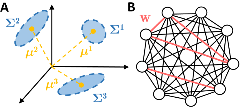
Figure 1: Model setup. (A) Real-world distribution modelled as several independent patterns following multivariate log-normal distribution. (B) Continuous Hopfield network with an example synaptic ensemble $\mathbf{w}$ (red) composed of four connections.

2.1 Coding of one synaptic connection

For a given pattern $\mathbf{x}^{k}$, the vector $\ln\mathbf{x}^{k}$ follows a multivariate Gaussian distribution. Consequently, its $i^{\mathrm{th}}$ component also follows a Gaussian distribution, denoted as $\ln\mathbf{x}^{k}_{i}\sim\mathcal{N}(\mathbf{\mu}^{k}_{i},(\sigma^{k}_{i})^{2})$, where the mean $\mathbf{\mu}^{k}_{i}$ is the $i^{\mathrm{th}}$ component of $\mathbf{\mu}^{k}$, and the variance $(\sigma^{k}_{i})^{2}$ is the $i^{\mathrm{th}}$ diagonal element of the covariance matrix $\Sigma^{k}$. Similarly, the sum of the $i^{\mathrm{th}}$ and $j^{\mathrm{th}}$ components follows a Gaussian distribution of the form:

$$\ln(\mathbf{x}^{k}_{i})+\ln(\mathbf{x}^{k}_{j})=\ln(\mathbf{x}^{k}_{i}\mathbf{x}^{k}_{j})\sim\mathcal{N}(\mathbf{\mu}^{k}_{i}+\mathbf{\mu}^{k}_{j},(\sigma^{k}_{i})^{2}+(\sigma^{k}_{j})^{2}+2\sigma^{k}_{ij}),$$ (2)

where $\sigma^{k}_{ij}$ represents the $(i,j)$ element of the covariance matrix $\Sigma^{k}$. Therefore, the random variable $\mathbf{x}^{k}_{i}\mathbf{x}^{k}_{j}$ also follows a log-normal distribution. The synaptic connection $w_{ij}=\sum_{k=1}^{N}\mathbf{x}^{k}_{i}\mathbf{x}^{k}_{j}$ is thus the sum of multiple independent log-normally distributed variables.

Fortunately, the problem of approximating the sum of log-normal variables has been extensively studied in the engineering field due to the prevalence of such noise in communication systems. One of the most well-established methods is the Fenton-Wilkinson approximation [25], which approximates the sum of log-normals with a new log-normal variable using a moment-matching method. We apply this approach to derive the distribution for a single synaptic connection. This leads to the following proposition:

Proposition 1.1. For $N$ independent log-normally distributed patterns $\{\mathbf{x}^{1},...,\mathbf{x}^{N}\}$, the distribution of the synaptic connection $w_{ij}=\sum_{k=1}^{N}\mathbf{x}^{k}_{i}\mathbf{x}^{k}_{j}$ in the Hopfield network can be approximately described using a new log-normal distribution:

$$p(w_{ij})\approx\frac{1}{w_{ij}\sigma_{w}\sqrt{2\pi}}\exp\left(-\frac{(\ln w_{ij}-\mu_{w})^{2}}{2\sigma_{w}^{2}}\right)$$ (3)

where the parameters $\mu_{w}$ and $\sigma_{w}^{2}$ are:

$$\mu_{w}=\ln M_{1}-\frac{1}{2}\ln(1+\frac{M_{2}}{M_{1}^{\ 2}}),\quad\sigma_{w}^{2}=\ln(1+\frac{M_{2}}{M_{1}^{\ 2}})$$ (4)

with $M_{1}$ and $M_{2}$ defined as:

$$M_{1}:=\sum_{k=1}^{N}\exp\left(\mathbf{\mu}^{k}_{i}+\mathbf{\mu}^{k}_{j}+\frac{1}{2}\left[(\sigma^{k}_{i})^{2}+(\sigma^{k}_{j})^{2}+2\sigma^{k}_{ij}\right]\right)$$ (5)

$$M_{2}:=\sum_{k=1}^{N}\left[\exp\left((\sigma^{k}_{i})^{2}+(\sigma^{k}_{j})^{2}+2\sigma^{k}_{ij}\right)-1\right]\exp\left(2(\mathbf{\mu}^{k}_{i}+\mathbf{\mu}^{k}_{j})+(\sigma^{k}_{i})^{2}+(\sigma^{k}_{j})^{2}+2\sigma^{k}_{ij}\right)$$ (6)

This provides us with the closed-form expression for $p(w_{ij})$. Furthermore, deriving the mutual information $MI(w_{ij};\mathbf{x}^{l})$ requires the conditional distribution $p(w_{ij}|\mathbf{x}^{l})$. Given the independence of the $N$ terms in a given weight, i.e., $\mathbf{x}^{k}_{i}\mathbf{x}^{k}_{j}\perp\mathbf{x}^{l}_{i}\mathbf{x}^{l}_{j}\ \forall k\neq l$, the distributions $p(w_{ij}|\mathbf{x}^{l})$ and $p\left(\sum_{k\neq l}^{N}\mathbf{x}^{k}_{i}\mathbf{x}^{k}_{j}\right)$ are isomorphic in the sense that the latter is a shifted version of the former by a constant $-\mathbf{x}^{l}_{i}\mathbf{x}^{l}_{j}$. Consequently, we can derive the probability distribution for $\sum_{k\neq l}^{N}\mathbf{x}^{k}_{i}\mathbf{x}^{k}_{j}$ instead, and the same derivation steps for $w_{ij}=\sum_{k}^{N}\mathbf{x}^{k}_{i}\mathbf{x}^{k}_{j}$ would apply. We denote this distribution by:

$$\ln w_{ij/l}:=\ln\left(\sum_{k\neq l}^{N}\mathbf{x}^{k}_{i}\mathbf{x}^{k}_{j}\right)\sim\mathcal{N}\left(\mu_{w/l},(\sigma_{w/l})^{2}\right),$$ (7)

where the parameters $\mu_{w/l}$ and $(\sigma_{w/l})^{2}$ have the same form as in Equation 4, with the $l^{\mathrm{th}}$ term removed from the summation in Equations 5 and 6.

With both $p(w_{ij})$ and $p(w_{ij}|\mathbf{x}^{l})$ known, we can obtain the analytical expression for the mutual information:

Proposition 1.2. The mutual information between a synaptic connection and a pattern is given by:

$$MI(w_{ij};\mathbf{x}^{l})=\left(\mu_{w}-\mu_{w/l}\right)+\left(\ln\sigma_{w}-\ln\sigma_{w/l}\right),$$ (8)

with the units in nats.

2.2 Coding for a pair of connections

Different synaptic connections within a neural network interact with each other and may influence coding beyond the information contained in a single connection. To study the collective coding paradigm of these connections, we focus on the mutual information between data and the joint activity of two connections, $MI(\mathbf{w};\mathbf{x}^{l})$, where $\mathbf{w}=(w_{ij},w_{mn})^{T}$. This analysis requires knowledge of the distributions $p(\mathbf{w})$ and $p(\mathbf{w}|\mathbf{x}^{l})$.

From the derivation in the single connection case, we obtain the marginals for each weight, which are given by:

$$\ln w_{ij}\sim\mathcal{N}\left(\mu_{w_{ij}},(\sigma_{w_{ij}})^{2}\right),\quad\ln w_{mn}\sim\mathcal{N}\left(\mu_{w_{mn}},(\sigma_{w_{mn}})^{2}\right),$$ (9)

where a new layer of subscripts ($ij,mn$) is added to $\mu_{w}$ and $\sigma_{w}$ from Equation 4 to distinguish the two different weights. This implies that the marginal distributions of the vector $\ln\mathbf{w}=(\ln w_{ij},\ln w_{mn})^{T}$ both follow a Gaussian distribution. Given the constraints provided by the marginals, we approximate the joint distribution for $\ln\mathbf{w}$ with a 2-dimensional Gaussian distribution. We express it as:

$$\ln\mathbf{w}=\begin{pmatrix}\ln w_{ij}\\ \ln w_{mn}\end{pmatrix}\sim\mathcal{N}(\mu_{\mathbf{w}}=\begin{pmatrix}\mu_{w_{ij}}\\ \mu_{w_{mn}}\end{pmatrix},\Sigma_{\mathbf{w}}=\begin{pmatrix}\sigma_{w_{ij}}^{2}&\sigma_{w_{ij,mn}}\\ \sigma_{w_{mn,ij}}&\sigma_{w_{mn}}^{2}\end{pmatrix}).$$ (10)

The only remaining unknown in this equation is $\sigma_{w_{ij,mn}}$, which represents the covariance between $\ln w_{ij}$ and $\ln w_{mn}$. The expression for this covariance is presented in the following proposition:

Proposition 2.1. For a pair of synaptic connections $(w_{ij},w_{mn})^{T}$ following a 2-dimensional log-normal distribution, the covariance between $\ln w_{ij}$ and $\ln w_{mn}$ is:

$$\sigma_{w_{ij,mn}}=\ln(1\;+$$

$$\frac{\sum_{k=1}^{N}\exp\left(\sum_{\phi}^{\{i,j,m,n\}}\mu^{k}_{\phi}+\frac{1}{2}\sum_{\phi}^{\{i,j,m,n\}}(\sigma^{k}_{\phi})^{2}+\sum_{\phi}^{\{ij,mn\}}\sigma^{k}_{\phi}\right)\left[\exp\left(\sum_{\phi}^{\{i,j\}\times\{m,n\}}\sigma^{k}_{\phi}\right)-1\right]}{\sum_{k,l=1}^{N}\exp\left(\sum_{\phi}^{\{i,j\}}\mu^{k}_{\phi}+\sum_{\phi}^{\{m,n\}}\mu^{l}_{\phi}+\frac{1}{2}\sum_{\phi}^{\{i,j\}}(\sigma^{k}_{\phi})^{2}+\frac{1}{2}\sum_{\phi}^{\{m,n\}}(\sigma^{l}_{\phi})^{2}+\sigma_{ij}^{k}+\sigma_{mn}^{l}\right)})$$ (11)

with the summation notation meaning:

$$\sum_{\phi}^{\{ij,mn\}}\sigma^{k}_{\phi}=\sigma^{k}_{ij}+\sigma^{k}_{mn}\;,\sum_{\phi}^{\{i,j\}\times\{m,n\}}\sigma^{k}_{\phi}=\sigma^{k}_{im}+\sigma^{k}_{in}+\sigma^{k}_{jm}+\sigma^{k}_{jn}$$ (12)

These derivations show how the distribution $p(\mathbf{w})$ can be approximated by a 2-dimensional log-normal distribution with derived parameter values. The next step is to study $p(\mathbf{w}|\mathbf{x}^{l})$. Similar to the single connection scenario, $p(\mathbf{w}|\mathbf{x}^{l})$ and $p\left(\sum_{k\neq l}^{N}\mathbf{x}^{k}_{i}\mathbf{x}^{k}_{j},\sum_{k\neq l}^{N}\mathbf{x}^{k}_{m}\mathbf{x}^{k}_{n}\right)$ are isomorphic distributions, with their domains shifted. Therefore, the same steps used to derive $p(\mathbf{w})$ apply here, leading to the following distribution:

$$\ln\mathbf{w}_{/l}:=\begin{pmatrix}\ln w_{ij/l}\\ \ln w_{mn/l}\end{pmatrix}\sim\mathcal{N}(\mu_{\mathbf{w}/l}=\begin{pmatrix}\mu_{w_{ij}/l}\\ \mu_{w_{mn}/l}\end{pmatrix},\Sigma_{\mathbf{w}/l}=\begin{pmatrix}\sigma_{w_{ij}/l}^{2}&\sigma_{w_{ij,mn/l}}\\ \sigma_{w_{mn,ij/l}}&\sigma_{w_{mn}/l}^{2}\end{pmatrix}),$$ (13)

where the parameters with $/l$ are equal to their original corresponding parameters, with the terms related to $\mathbf{x}^{l}$ removed from the summation. For a more detailed expression, please refer to the Methods section.

Given $p(\mathbf{w})$ and $p(\mathbf{w}|\mathbf{x}^{l})$, we can then calculate the mutual information encoded in any pair of synaptic connections and a data pattern, as stated in the following proposition:

Proposition 2.2. The mutual information between a pair of connections $\mathbf{w}=(w_{ij},w_{mn})^{T}$ and a data pattern $\mathbf{x}^{l}$ is given by:

$$MI(\mathbf{w};\mathbf{x}^{l})=(\mu_{w_{ij}}+\mu_{w_{mn}}-\mu_{w_{ij}/l}-\mu_{w_{mn}/l})+\frac{1}{2}\ln|\Sigma_{\mathbf{w}}|-\frac{1}{2}\ln|\Sigma_{\mathbf{w}/l}|,$$ (14)

where $|\Sigma_{\mathbf{w}}|$ denotes the determinant of the matrix $\Sigma_{\mathbf{w}}$. The information is expressed in nats.

2.3 Information in an ensemble of multiple synaptic connections

The next step is to extend the analysis to the case of information encoded jointly in an ensemble of $n$ synaptic connections, denoted as $\mathbf{w}=(w_{ij(1)},w_{ij(2)},\dots,w_{ij(n)})^{T}$. Here, the set $\{ij(1),ij(2),\dots,ij(n)\}$ represents the indices for the $n$ synaptic weights. For example, $w_{ij(k)}$ refers to the connection between neuron $i(k)$ and neuron $j(k)$. The mutual information encoded by any $n$ connections about the data, $MI(\mathbf{w};\mathbf{x}^{l})$, can be derived using a similar approach as before. Since all marginals for $\ln\mathbf{w}$ are normally distributed, we approximate the distribution as an $n$-dimensional log-normal distribution, leading to:

$$\ln\mathbf{w}=\begin{pmatrix}\ln w_{ij(1)}\\ \vdots\\ \ln w_{ij(n)}\end{pmatrix}\sim\mathcal{N}(\mu_{\mathbf{w}}=\begin{pmatrix}\mu_{w_{ij(1)}}\\ \vdots\\ \mu_{w_{ij(n)}}\end{pmatrix},\Sigma_{\mathbf{w}}=\begin{pmatrix}\sigma_{w_{ij(1)}}^{2}&\sigma_{w_{ij(1),ij(2)}}&\ldots&\sigma_{w_{ij(1),ij(n)}}\\ \sigma_{w_{ij(2),ij(1)}}&\sigma_{w_{ij(2)}}^{2}&\ldots&\sigma_{w_{ij(2),ij(n)}}\\ \vdots&\vdots&\ddots&\vdots\\ \sigma_{w_{ij(n),ij(1)}}&\sigma_{w_{ij(n),ij(2)}}&\ldots&\sigma_{w_{ij(n)}}^{2}\end{pmatrix})$$ (15)

This expression represents $p(\mathbf{w})$ as an $n$-dimensional log-normal distribution. The parameters $\mu_{\mathbf{w}}$ and the diagonal elements of $\Sigma_{\mathbf{w}}$ follow the form given in Equation 4, while the off-diagonal elements of $\Sigma_{\mathbf{w}}$ follow Equation 11, specifically:

$$\sigma_{w_{ij(r),ij(s)}}=\ln(1\;+$$

$$\frac{\sum_{k=1}^{N}\exp\left(\sum_{m}^{\{r,s\}}\left[\sum_{\phi}^{\{i(m),j(m)\}}\mu^{k}_{\phi}+\frac{1}{2}(\sigma^{k}_{\phi})^{2}\right]+\sigma^{k}_{ij(m)}\right)\left[\exp\left(\sum_{\phi}^{\{i(r),j(r)\}\times\{i(s),j(s)\}}\sigma^{k}_{\phi}\right)-1\right]}{\sum_{k,l=1}^{N}\exp\left(\left[\sum_{\phi}^{\{i(r),j(r)\}}\mu^{k}_{\phi}+\frac{1}{2}(\sigma^{k}_{\phi})^{2}\right]+\;\left[\sum_{\phi}^{\{i(s),j(s)\}}\mu^{l}_{\phi}+\frac{1}{2}(\sigma^{l}_{\phi})^{2}\right]+\sigma_{ij(r)}^{k}+\sigma_{ij(s)}^{l}\right)})$$ (16)

To obtain $p(\mathbf{w}|\mathbf{x}^{l})$, as in the single and double connection scenarios, we focus on its isomorphic distribution $p(\mathbf{w}_{/l})$, which is also log-normally distributed. The parameters with $/l$ are simply the original parameters with the summation terms related to $\mathbf{x}^{l}$ excluded:

$$\ln\mathbf{w}_{/l}=\begin{pmatrix}\ln w_{ij(1)/l}\\ \vdots\\ \ln w_{ij(n)/l}\end{pmatrix}\sim\mathcal{N}(\mu_{\mathbf{w}/l}=\begin{pmatrix}\mu_{w_{ij(1)}/l}\\ \vdots\\ \mu_{w_{ij(n)}/l}\end{pmatrix},\Sigma_{\mathbf{w}/l}=\begin{pmatrix}\sigma_{w_{ij(1)}/l}^{2}&\ldots&\sigma_{w_{ij(1),ij(n)}/l}\\ \vdots&\ddots&\vdots\\ \sigma_{w_{ij(n),ij(1)}/l}&\ldots&\sigma_{w_{ij(n)}/l}^{2}\end{pmatrix})$$ (17)

Finally, with $p(\mathbf{w})$ and $p(\mathbf{w}|\mathbf{x}^{l})$, we can derive the analytical expression for the information jointly encoded in multiple synaptic connections about a pattern:

Proposition 3. The mutual information between the joint activity of $n$ synaptic connections $\mathbf{w}=(w_{ij(1)},w_{ij(2)},...,w_{ij(n)})^{T}$ and a data pattern $\mathbf{x}^{l}$ is:

$$MI(\mathbf{w};\mathbf{x}^{l})=\sum_{k=1}^{n}\left(\mu_{w_{ij(k)}}-\mu_{w_{ij(k)}/l}\right)+\frac{1}{2}\ln|\Sigma_{\mathbf{w}}|-\frac{1}{2}\ln|\Sigma_{\mathbf{w}/l}|$$ (18)

3 Results

After obtaining the analytical solution for the information encoded in synaptic connections, we performed a series of exploratory analyses to see if any interesting patterns emerged. We began with simple, special cases where most parameters were fixed, then progressed to more general cases involving multiple variable parameters.

From our derivation, we observe that the mutual information (MI) between an ensemble of synaptic connections $\mathbf{w}=(w_{ij(1)},...,w_{ij(n)})^{T}$ and a data pattern $\mathbf{x}^{l}$ , denoted $MI(\mathbf{w};\mathbf{x}^{l})$, depends on the distribution properties of each data pattern, specifically their means and covariance matrices, as well as the set of connections selected for $\mathbf{w}$. This is because, given the fixed relationship $w_{ij}=\sum_{k}\mathbf{x}^{k}_{i}\mathbf{x}^{k}_{j}$ in a Hopfield network, the distribution of $\mathbf{w}$ can be determined from the distribution of data patterns. Notably, we found that the information encoded in any given ensemble does not depend on the dimensionality of the data pattern, $d$, which also represents the size of the Hopfield network. This is because each weight $w_{ij}=\sum_{k}\mathbf{x}^{k}_{i}\mathbf{x}^{k}_{j}$ involves only the two corresponding components $i$ and $j$, with the other components having no effect. As a result, the parameter $d$ does not appear in the expression for mutual information. Therefore, we fix $d=20$ in all subsequent analyses and simulations, though the same results should hold for larger $d$ values.

We conducted three sets of simulations, varying both the distribution of data patterns and the number of synaptic connections in the ensemble, each with increasingly higher degrees of freedom. While mutual information (MI) in the theoretical section is measured in nats for mathematical elegance, in the following simulation and analysis sections, MI is expressed in bits to provide a more intuitive understanding of the quantity of information.

First Simulation Set: Here, all patterns shared the same covariance matrix, with only the mean values of the distributions differing. The covariance matrices were exchangeable, with diagonal elements set to $\tilde{\sigma}^{2}$ and off-diagonal elements to $\tilde{\rho}\tilde{\sigma}^{2}$. We studied how the mutual information between a given set of synaptic connections and a data pattern varied with respect to parameters such as $\tilde{\rho},\tilde{\sigma}$, the number of data patterns, and the number of connections, using an example set of synaptic connections and pattern mean values.

Second Simulation Set: In this case, the patterns still shared the same covariance matrix, but we relaxed the assumption of exchangeability by introducing a more general case involving a stochastic matrix $\mathbf{A}$, where $\mathbf{A}^{T}\mathbf{A}/d$ was added to the covariance structure. Additionally, the pattern means and synaptic connections were sampled stochastically, leading to varying mutual information values. We visualized these changes using scatter plots and performed regression analysis to identify the factors affecting mutual information.

Third Simulation Set: In this final set, the patterns were allowed to have different covariance matrices. To avoid bias in the covariance matrix generation, we constructed random covariance matrices by generating random eigenvalues and random orthogonal matrices. As in the second set, other parameters were sampled stochastically. We again used scatter plots and regression analysis to examine the results.

For more detailed information regarding the simulation procedures, please refer to the Materials and Methods section.

3.1 Information about each pattern decreases as the total number of patterns increases

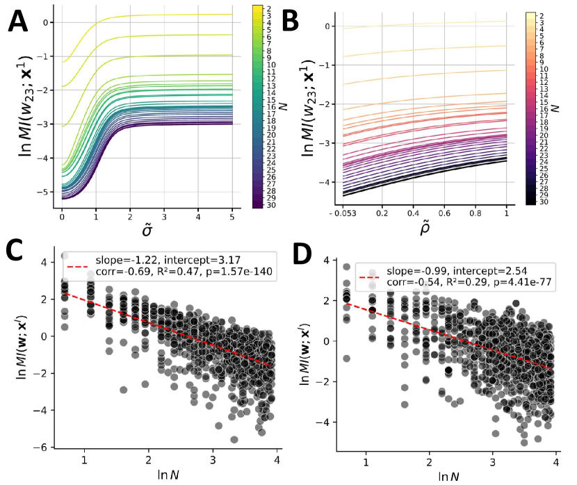
Figure 2: Information and the number of data patterns. For each $N$, the curves show how the information encoded in a single example weight varies with (A) $\tilde{\sigma}$ and (B) $\tilde{\rho}$. As $N$ increases, the overall curves shift downward, indicating a decrease in the total information encoded. This decreasing trend is significant for randomly sampled distribution configurations with (C) the same covariance matrix and (D) different covariance matrices.

The results from the first simulation set show how the information encoded in a single synaptic connection, specifically $MI(\mathbf{x}^{1};w_{23})$, changes as a function of $\tilde{\sigma}$ when $\tilde{\rho}=0$ (Fig. 2A) and as a function of $\tilde{\rho}$ when $\tilde{\sigma}=1$ (Fig. 3A). Curves for varying numbers of data patterns (ranging from 2 to 30) are plotted together for comparison. As shown in Figs. 1A and 1B, the information encoded in a single connection—represented here by $MI(\mathbf{x}^{1};w_{23})$—increases with both $\tilde{\sigma}$ and $\tilde{\rho}$.

A plausible explanation is that $\tilde{\sigma}$ represents the spread or width of the distribution, and a wider distribution typically corresponds to higher entropy in the data patterns, thus providing more content for the network to encode. Meanwhile, $\tilde{\rho}$ reflects the internal structure of the data; data with more structure tends to be easier for the network to store, assuming the same level of entropy. However, as the number of data patterns increases from 2 to 30, $MI(\mathbf{x}^{1};w_{23})$ decreases, as evidenced by the downward shift of the curve on a logarithmic scale. This suggests that the information stored in each individual connection about a single data pattern decreases as the total number of patterns to be stored in the neural network increases, rather than remaining constant.

This pattern of decrease is also evident in the second (Fig. 2C) and third (Fig. 2D) simulation sets, where the covariance matrix is not restricted to be exchangeable, and the synaptic ensemble may stochastically include more than one connection. In these cases, we compute the information $MI(\mathbf{w};\mathbf{x}^{l})$, where $\mathbf{w}$ is an ensemble of $n$ randomly selected weights, and $n$ itself is also random. $\mathbf{x}^{l}$ represents a pattern randomly chosen from all $N$ patterns. Each point in the scatter plots corresponds to an $MI$ value generated from a single sampling of all parameters.

In Fig. 2C, where the covariance matrices are identical across patterns, we observe a significant negative correlation between $MI(\mathbf{w};\mathbf{x}^{l})$ and $N$, with a correlation coefficient of -0.69 ($p=1.57\times 10^{-140}$, $R^{2}=0.47$). This trend holds in Fig. 2D, where the covariance matrices differ between patterns, with a correlation coefficient of -0.54 ($p=4.41\times 10^{-77}$, $R^{2}=0.29$). Furthermore, by examining the slope of the linear relationship between $\ln(MI(\mathbf{w};\mathbf{x}^{l}))$ and $\ln(N)$, we find that $MI(\mathbf{w};\mathbf{x}^{l})$ follows an approximate $N^{-1.2}$ scaling in Fig. 2C and $N^{-1.0}$ in Fig. 2D.

3.2 Relation between the number of synaptic connections and information in an ensemble

Next, we examine how mutual information changes in relation to the number of synaptic connections, rather than the number of data patterns. For the analysis based on the first simulation set, the number of data patterns is fixed at $N=10$. Results are shown in Fig. 3A for varying $\tilde{\sigma}$ ($\tilde{\rho}=0$) and Fig. 3B for varying $\tilde{\rho}$ ($\tilde{\sigma}=1$). The mutual information between the joint activity of an example synaptic ensemble and a data pattern, $MI(\mathbf{w};\mathbf{x}^{1})$, is plotted. Similar to the case with a single synaptic connection, the trend of increasing $MI(\mathbf{w};\mathbf{x}^{1})$ with $\tilde{\sigma}$ and $\tilde{\rho}$ holds true for an ensemble of synaptic connections. Additionally, as shown by the curves in different colors in Figs. 2A and 2B, the information in the ensemble increases with the number of connections, $n$. This result is expected since adding more variables should not decrease the total information.

However, in Fig. 3B, for ensembles with five or more connections, we observe that the curves may abruptly rise, producing NaN or infinite values when the correlation $\tilde{\rho}$ becomes large. As a result, we did not plot the curve beyond the point where the first NaN or infinite value appears. This issue stems from an approximation made in assuming that $\mathbf{w}$ follows a multivariate log-normal distribution. The estimated covariance matrix $\Sigma_{\mathbf{w}}$ may deviate from positive definiteness as the data pattern distributions approach singularity with increasing correlation among components. This can cause the determinant of $\Sigma_{\mathbf{w}}$ to approach zero or become negative, which prevents the computation of mutual information because it involves the term $\ln|\Sigma_{\mathbf{w}}|$. To address this, we applied an extrapolation method to fill in the missing values, preventing bias in the distribution caused by these gaps. Details on the extrapolation method can be found in the Materials and Methods section.

The results from simulation set two (Fig. 3C) and simulation set three (Fig. 3D) provide further quantitative insights into the relationship between $MI(\mathbf{w};\mathbf{x}^{l})$, where $\mathbf{w}$, $l$, and the data pattern distributions are all randomly sampled. In both cases, a significant positive relationship is observed, with correlation coefficients of 0.61 ($p=2.35\times 10^{-104}$, $R^{2}=0.38$) for Fig. 3C and 0.59 ($p=9.10\times 10^{-97}$, $R^{2}=0.35$) for Fig. 3D.

Moreover, the slope of the linear regression shows consistent results across both analyses, indicating a relationship of $MI(\mathbf{w};\mathbf{x}^{l})\sim n^{1.1}$. This suggests a general equation linking the amount of encoded information to the size of any ensemble of synaptic connections. In a special case where the synaptic ensemble includes the full connectivity of a Hopfield network with $d$ neurons, we note that $MI\sim d^{2.2}$, which follows directly from the fact that the number of connections $n\sim d^{2}$. Since the dimension of the data pattern is $d$, and successfully storing a pattern would require a proportional amount of information, the total information needed for successful memorization should scale with $d$. From this, we can estimate that the number of patterns a Hopfield network can store, based on the synaptic connections, should follow $P\sim d^{1.2}$, where $P$ denotes the number of stored patterns.

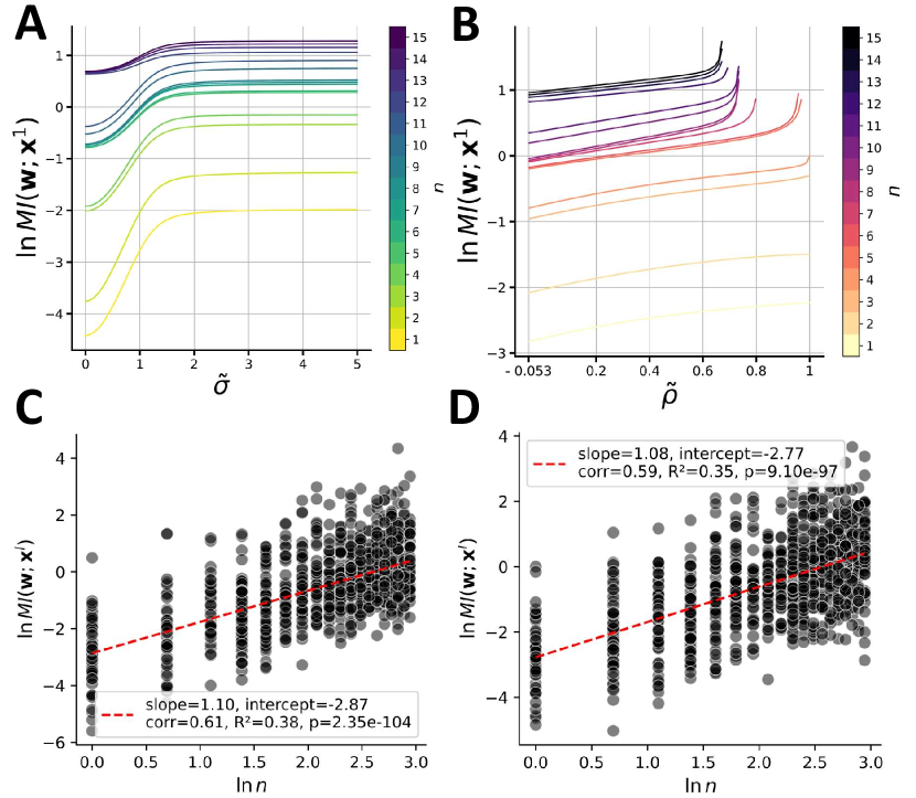
Figure 3: Information and the number of synaptic connections in an ensemble. For each $n$, the curves show how the information encoded in an example ensemble varies with (A) $\tilde{\sigma}$ and (B) $\tilde{\rho}$. As $n$ increases, the overall curves shift upward, indicating an increase in the total information encoded. This increasing trend also holds significant for randomly sampled distribution configurations with (C) the same covariance matrix and (D) different covariance matrices.

3.3 Information contributed per connection increases with the synaptic ensemble size

In the previous sections, we analyzed the information encoded by a single synaptic connection, $MI(w;\mathbf{x}^{l})$, and by an ensemble of synaptic connections, $MI(\mathbf{w},\mathbf{x}^{l})$. However, an intriguing question arises: how does the information encoded by a single connection on its own compare to its contribution as part of a larger ensemble? To address this, we approximated the contribution of a single connection within an ensemble as $MI(\mathbf{w},\mathbf{x}^{l})/n$, where $n$ is the size of the ensemble. This comparison sheds light on how individual connections behave differently when functioning independently versus as part of a collective.

Using data from simulation set three, which reflects the most general distribution, we computed the relationship between $\ln(MI(\mathbf{w},\mathbf{x}^{l})/n)$ and $n$. As shown in the histogram in Figure 4B, $\ln(MI(\mathbf{w},\mathbf{x}^{l})/n)$ follows a Gaussian-like distribution, which shifts toward higher values as $n$ increases. This indicates a notable change in the distribution, as evidenced by significant differences between $n=1$ and $n=4$ ($p=5.7\times 10^{-5}$, two-sided t-test) and between $n=4$ and $n=16$ ($p=8.5\times 10^{-5}$, two-sided t-test).

To further explore this relationship, we plotted the mean and standard deviation of $\ln(MI(\mathbf{w},\mathbf{x}^{l})/n)$ for each value of $n$, and performed a linear regression analysis. As shown in Figure 4A, there is a significant positive correlation between the mean and $n$ (correlation coefficient = 0.70, $p=8.55\times 10^{-4},R^{2}=0.49$). Similarly, there is a significant negative correlation between the standard deviation and $n$ (correlation coefficient = -0.62, $p=4.69\times 10^{-3},R^{2}=0.38$). These findings suggest that the information contributed per synaptic connection increases with ensemble size, while the variability of this contribution decreases for larger ensembles.

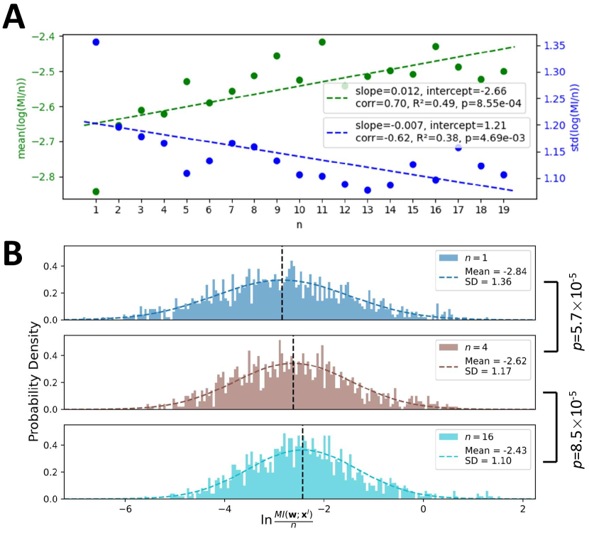
Figure 4: Information contributed per synaptic connection as a function of ensemble size. (A) The relationship between $n$ and the mean (green, left axis) as well as standard deviation (blue, right axis) of $\ln(MI/n)$. (B) Histograms showing the distribution of $\ln(MI/n)$ for $n=1,4,9,16$.

4 Discussion

In this study, we adopted a less conventional and under-explored perspective on neural coding, focusing on the information encoded in synaptic weights rather than in neuronal firing activities. As an initial step in this direction, our objective was to derive an analytical solution for the mutual information encoded in ensembles of synaptic connections. This allows us to compute the information directly from the expression, eliminating the need for extensive numerical simulations typically required for estimating mutual information. Using a continuous Hopfield network and assuming a log-normal distribution, we successfully derived a closed-form expression. Although this formulation may initially seem complex, we believe it might represent the simplest possible analytical solution for this problem. With this expression, we conducted three sets of simulations, revealing interesting insights into distributed coding, network capacity, and information synergy, which are discussed in detail in the following sections. Overall, we propose that our work provides a framework for analyzing neural information through the lens of synaptic connections, offering a complementary perspective to the traditional focus on firing activities.

4.1 Distributed coding in synaptic weights

We have demonstrated that the mutual information about a data pattern, whether stored in a single synaptic weight, $MI(w_{ij};\mathbf{x}^{1})$, or an ensemble of synaptic weights, $MI(\mathbf{w};\mathbf{x}^{l})$, decreases as the number of stored patterns $N$ increases. This suggests that introducing new patterns for storage reduces the capacity of synaptic connections to retain information about previously stored patterns. In other words, each synaptic connection allocates part of its storage capacity to every new pattern, resulting in a scenario where each connection simultaneously encodes partial information about all stored patterns. This is in contrast to a potential alternative where certain synapses would specialize in encoding specific patterns while others specialize in different ones. Our findings align with the well-known paradigm of distributed coding in the brain, where diverse types of information—such as memory [26], sensory inputs [27], or motor actions [28]—are encoded collectively across groups of neurons. Notably, our analysis provides support for this phenomenon from the perspective of synaptic connections within neural networks.

4.2 Capacity Analysis for the Hopfield Network

Our work has also examined the capacity of the Hopfield network based on the information stored within synaptic ensembles. In this study, we employed the continuous version of the Hopfield network, where both data patterns and weights can take values across a continuous range. Unlike the well-studied discrete version, where the network’s capacity has been extensively explored, little attention has been given to the continuous case. [29] suggested that, for the continuous version, capacity becomes theoretically infinite due to the infinite entropy of continuous random variables. However, we have demonstrated that the mutual information between a continuous weight and a continuous pattern is finite, offering a new perspective on this problem. By assuming that each component or ”digit” in a pattern requires the same amount of information, we found that the number of stored patterns follows a slightly superlinear relationship with the size of the Hopfield network, i.e., $P\sim d^{1.2}$. This is analogous to previous work on the discrete Hopfield network, such as $P\sim 0.14d$ [30] or $P\leq d$ [29]. These results suggest that similar storage laws might apply to the continuous version of the Hopfield network.

The discrepancy between our finding of $P\sim d^{1.2}$ and the previously reported $P\sim d$ can be attributed to fundamentally different approaches in deriving storage capacity. In traditional methods, capacity is evaluated by calculating the number of patterns that can be successfully retrieved based on the dynamics of neuron firing activity. In contrast, our method focuses on the patterns directly stored in the connectivity. In other words, the distinction lies in comparing patterns encoded in the synaptic weights with those that can be retrieved through neural dynamics. Given that the information flow in the learning paradigm of the Hopfield network can be conceptualized as a Markov chain, where data pass through connectivity before being retrieved by dynamics, the data processing inequality suggests that the mutual information between the data and connections should exceed that of the retrieval dynamics. Thus, we believe that the observed superlinear capacity result reflects the information loss in the retrieval phase.

Additionally, our approach offers a more general perspective by revealing the relationship between information and synaptic ensemble size, $MI\sim n^{1.1}$. Unlike traditional studies that focus on storage capacity in the full $d\times d$ Hopfield network, our method applies to any selected connection ensemble within the network, including different motifs. This generalization provides a framework for future investigations into neural information coding. Traditional approaches face limitations when subsets of connections within a $d\times d$ network fail to cover all components of a pattern, complicating the definition of successful pattern retrieval. Thus, we believe that our method offers a complementary viewpoint that addresses gaps in traditional approaches.

4.3 Synergy among synaptic connections

We have demonstrated that the connections in a network can jointly encode more information than the sum of individual synaptic connections, i.e., $\mathbb{E}[MI(\mathbf{w};\mathbf{x}^{l})]>n\mathbb{E}[MI(w;\mathbf{x}^{l})]$. This phenomenon, where the whole is greater than the sum of its parts, is known as information synergy. Synergy has been a longstanding topic in neuroscience, with evidence of its existence in the coding of systems such as neurons [31, 32] and brain regions [33]. However, our approach provides novel evidence of synergy at the level of synaptic connections.

Synergy in neural coding arises due to interactions among components of the system. These interactions can occur at various levels: pairwise, triplet, quadruplet, or even higher-order interactions. Classical studies of synergistic coding in neurons often focus on the role of correlations between spikes, which represent second-order interactions. More recent work has explored third-order interactions, introducing concepts such as triplet correlations [34]. By deriving closed-form expressions for Shannon mutual information, our work offers a straightforward way to analyze higher-order interactions by calculating $MI(\mathbf{w};\mathbf{x}^{l})/n$, the contribution of a single connection to the encoding of the ensemble. In our simulations, we estimated interactions ranging from second to nineteenth order using this value and observed a significant increasing trend as the number of connections $n$ grew. This suggests that synergistic effects extend at least to the 19th order, indicating that further insights may await discovery at higher orders.

Nevertheless, it remains unclear whether this synergistic scenario will continue indefinitely as interaction orders increase. Some studies suggest that synergistic effects dominate only at smaller neural populations, typically involving fewer than 200 neurons, while coding becomes increasingly redundant at larger scales [35]. Indeed, our analysis did not reach the scale of $n>40,000$ synaptic connections due to computational limitations. Additionally, the linear regression results in Figure 4A suggest a relationship of $MI\sim ne^{0.012n}$, which would imply an exponentially growing storage capacity as the ensemble size increases. This outcome would sharply contrast with established results for Hopfield networks. Therefore, we expect that the linear trend seen in Figure 4A will eventually plateau or saturate as $n$ becomes large.

This observation leads to an intriguing question: what is the optimal size for neurons or synaptic connections to maximize synergy? Identifying this ”most synergistic” size may point to a fundamental unit of neural coding and is a promising direction for future research.

4.4 Assumptions and considerations

We employed the continuous Hopfield network with Hebbian-like connectivity for its mathematical tractability. More commonly used architectures, such as multi-layer fully connected networks or recurrent neural networks, were not covered in this study. Additionally, biological neural networks possess greater complexity than that captured by the Hopfield network model. Despite these constraints, the Hopfield network remains a valuable model due to its foundational role in associative memory and neural information storage. Indeed, it has been successfully applied to various brain regions, including the hippocampus [36, 37], prefrontal cortex [38], primary visual cortex [39], and olfactory bulb [40], suggesting that insights from this model may apply more generally. Consequently, our framework represents an important step forward in characterizing information storage in synaptic connections.

The assumption of log-normal distributions for the data may appear restrictive at first glance, as it implies positivity in the data. However, Shannon mutual information is invariant under smooth, bijective transformations such as translation and scaling [41], allowing negative values to be incorporated into the data without altering the mutual information. As long as the true underlying distribution can be smoothly transformed to a log-normal form, our analysis holds. Consequently, our results are plausibly robust for any unimodal, skewed distribution with long tails, as these are the key properties that remain intact under such transformations. For more general unimodal distributions, our approach should still provide a reasonable approximation through the construction of a minimally skewed log-normal distribution. Furthermore, it is well established that many forms of natural data, such as images [42], sounds [43], and language [44], exhibit unimodality, skewness, and long tails. These characteristics suggest that our framework offers broadly applicable insights into how synaptic connections encode information, beyond the specific assumptions of the model.

5 Methods

5.1 Parameter setup for simulation

In this section, we provide a detailed explanation of the three sets of simulations used in our analyses:

First Simulation Set: We generated $N$ distributions for all data patterns, $\{\mathbf{x}^{1},\dots,\mathbf{x}^{N}\}$, where each pattern is a $d$-dimensional random variable following an independent distribution $\ln(\mathbf{x}^{k})\sim\mathcal{N}(\mathbf{\mu}^{k},\Sigma^{k})$. The dimension $d=20$. The parameters $\{\mu^{1},\dots,\mu^{N}\}$ were sampled such that each component was drawn from a uniform distribution between -1 and 1. The covariance matrices were identical for all patterns and modeled as exchangeable:

$$\Sigma^{1}=\Sigma^{2}=...=\Sigma^{N}=\begin{pmatrix}\tilde{\sigma}^{2}&\tilde{\rho}\tilde{\sigma}^{2}&\ldots&\tilde{\rho}\tilde{\sigma}^{2}\\ \tilde{\rho}\tilde{\sigma}^{2}&\tilde{\sigma}^{2}&\ldots&\tilde{\rho}\tilde{\sigma}^{2}\\ \vdots&\vdots&\ddots&\vdots\\ \tilde{\rho}\tilde{\sigma}^{2}&\tilde{\rho}\tilde{\sigma}^{2}&\ldots&\tilde{\sigma}^{2}\end{pmatrix}.$$

We varied the parameters across different analyses. In Figure 2A, we set $\tilde{\rho}=0$ and varied the values of $N$ and $\tilde{\sigma}$, calculating the corresponding $MI(\mathbf{x}^{1};w_{23})$. In Figure 2B, $\tilde{\sigma}=1$ while $N$ and $\tilde{\rho}$ were varied, and $MI(\mathbf{x}^{1};w_{23})$ was computed. Note that the covariance matrix’s semi-definiteness requires $\frac{-1}{d-1}\leq\tilde{\rho}\leq 1$. In Figure 3A, we set $N=10$, $\tilde{\rho}=0$, and varied the size $n$ of the synaptic ensemble $\mathbf{w}$, incrementing by adding random new connections step by step while varying $\tilde{\sigma}$. The corresponding $MI(\mathbf{x}^{1};\mathbf{w})$ was computed. In Figure 3B, with $N=10$, $\tilde{\sigma}=1$, and $n$ varied similarly, $\tilde{\rho}$ was altered within $\frac{-1}{d-1}\leq\tilde{\rho}\leq 1$, and $MI(\mathbf{x}^{1};\mathbf{w})$ was computed.

Second Simulation Set: In this set, instead of varying parameters to plot curves, all distribution parameters were sampled randomly. The objective was to sample multiple distribution-information tuples, i.e., $\left(\{\mathbf{x}^{1},\dots,\mathbf{x}^{N}\},\mathbf{w},MI(\mathbf{w};\mathbf{x}^{l})\right)$, and analyze potential relationships between $MI$ and distribution parameters based on these samples. The dimension was set to $d=20$, and the number of patterns $N$ was randomly selected from 2 to 50 with equal probability. The parameters $\{\mu^{1},\dots,\mu^{N}\}$ were sampled from a uniform distribution between -1 and 1 for each component. The covariance matrices were identical for all patterns but more general than the previous set:

$$\Sigma^{1}=\Sigma^{2}=...=\Sigma^{N}=\mathbf{A}^{T}\mathbf{A}/d+\begin{pmatrix}\tilde{\sigma}^{2}&\tilde{\rho}\tilde{\sigma}^{2}&\ldots&\tilde{\rho}\tilde{\sigma}^{2}\\ \tilde{\rho}\tilde{\sigma}^{2}&\tilde{\sigma}^{2}&\ldots&\tilde{\rho}\tilde{\sigma}^{2}\\ \vdots&\vdots&\ddots&\vdots\\ \tilde{\rho}\tilde{\sigma}^{2}&\tilde{\rho}\tilde{\sigma}^{2}&\ldots&\tilde{\sigma}^{2}\end{pmatrix}.$$

Here, $\tilde{\sigma}$ was drawn from the absolute values of a standard normal distribution, and $\tilde{\rho}$ was sampled from a uniform distribution in the range $[\frac{-1}{d-1},1]$. The matrix $\mathbf{A}$ is stochastic, with each element sampled from a standard normal distribution. Both components, $\mathbf{A}^{T}\mathbf{A}/d$ and the exchangeable covariance matrix, are positive semi-definite, ensuring that their sum is a valid covariance matrix. The introduction of $\mathbf{A}^{T}\mathbf{A}/d$ adds degrees of freedom, but it tends to produce matrices with larger diagonal elements, potentially neglecting distributions with highly correlated components. In contrast, the original exchangeable matrix can capture high correlations between components due to its structure, but it lacks sufficient degrees of freedom to account for more complex variability in the data. By combining these two components, the resulting covariance matrix strikes a balance: the exchangeable matrix preserves the ability to model correlations, while the addition of $\mathbf{A}^{T}\mathbf{A}/d$ introduces more flexibility, allowing the matrix to capture a wider range of data patterns. This combination mitigates the limitations of both approaches, providing a richer and more balanced representation of the underlying data distributions. The $1/d$ scaling factor was designed to prevent either component from dominating.

Using this setup, we generated 1000 samples of $\left(\{\mathbf{x}^{1},\dots,\mathbf{x}^{N}\},\mathbf{w},MI(\mathbf{w};\mathbf{x}^{l})\right)$. When $MI(\mathbf{w};\mathbf{x}^{l})$ was invalid (e.g., NaN or infinite), an extrapolation method was used (see Section 5.2). For Figure 2C, we analyzed the regression between $MI$ and $N$. For Figure 3C, we analyzed the regression between $MI$ and $n$.

Third Simulation Set: The third set of simulations follows a similar approach to the second, where we sampled numerous distribution-information tuples $\left(\{\mathbf{x}^{1},\dots,\mathbf{x}^{N}\},\mathbf{w},MI(\mathbf{w};\mathbf{x}^{l})\right)$. The dimension was set to $d=20$, and the number of patterns $N$ was randomly selected from 2 to 50 with equal probability. The parameters $\{\mu^{1},\dots,\mu^{N}\}$ were sampled from a uniform distribution between -1 and 1 for each component. The key difference is that the covariance matrices varied across patterns:

$$\Sigma^{k}=\mathbf{Q}\mathbf{\Lambda}\mathbf{Q}^{T}+r\mathbf{1}\mathbf{1}^{T}.$$

Here, $\mathbf{Q}$ is a random orthogonal matrix generated via QR decomposition of a matrix whose elements were drawn from a standard normal distribution, and $\mathbf{\Lambda}$ is a diagonal matrix with random positive eigenvalues sampled from a normal distribution (mean 0.01, standard deviation 1.2). The scalar factor $r$ was sampled from a uniform distribution in the range [0, 1.44]. Similar to the second simulation set, by combining these two elements, we were able to capture both the flexibility offered by $\mathbf{Q}\mathbf{\Lambda}\mathbf{Q}^{T}$ and the structure in $\mathbf{1}\mathbf{1}^{T}$ needed to model strong correlations across components.

We initially generated 1000 samples. In Figure 2D, we analyzed the regression between $MI$ and $N$, while in Figure 3D, the regression was between $MI$ and $n$. Additionally, 20,000 samples were generated for the analysis of $MI/n$ in Figure 4. For all cases, we applied the extrapolation method to handle any invalid $MI$ values.

5.2 Extrapolation method for simulation

For the dataset of samples $\left(\{\mathbf{x}^{1},\dots,\mathbf{x}^{N}\},\mathbf{w},MI(\mathbf{w};\mathbf{x}^{l})\right)$, when the mutual information value in a sample is invalid—when it results in NaN or infinity due to approximation errors—we apply an extrapolation technique. This involves identifying another sample most similar to the current one and using its MI value as an extrapolated substitute.

To measure similarity between samples, we calculate the Euclidean distance based on six key features of $\left(\{\mathbf{x}^{1},\dots,\mathbf{x}^{N}\},\mathbf{w}\right)$, which capture the most prominent characteristics of each sample. The six features are:

1. Number of data patterns ($N$);

2. Size of the synaptic ensemble ($n$);

3. Pattern centroid dispersion ($q_{1}=\sum_{k}(\mu^{k}-\frac{1}{N}\sum_{i}{\mu^{i}})^{2}$), which reflects the spread of the pattern centroids;

4. Average determinant of covariance matrices ($q_{2}=\frac{1}{N}\sum_{k}|\Sigma^{k}|$), representing the overall breadth of the pattern distributions;

5. Average ratio of the largest to smallest eigenvalues ($q_{3}=\frac{1}{N}\sum_{k}(\lambda^{k}_{\mathrm{max}}/\lambda^{k}_{\mathrm{min}})$), which reflects the degree of data ”stretching” or elongation;

6. Correlation ratio ($q_{4}=\frac{1}{N}\frac{\sum_{i\neq j}|\Sigma^{k}_{ij}|}{\sum_{i=j}|\Sigma^{k}_{ij}|}$), representing the average ratio between the sum of off-diagonal elements and diagonal elements, which indicates the correlation structure of the pattern distributions.

Before computing the similarity between samples, we normalize these six features— $(N,n,q_{1},q_{2},q_{3},q_{4})$—to account for differences in their inherent scales. This normalization ensures that each feature contributes equally to the distance calculation. In the datasets used for our analyses, approximately 1% of the samples were generated using this extrapolation method.

5.3 Proofs for propositions

Proposition 1.1. For $N$ independent log-normally distributed patterns $\{\mathbf{x}^{1},...,\mathbf{x}^{N}\}$, the distribution of the synaptic connection $w_{ij}=\sum_{k=1}^{N}\mathbf{x}^{k}_{i}\mathbf{x}^{k}_{j}$ in the Hopfield network can be approximately described using a new log-normal distribution:

$$p(w_{ij})\approx\frac{1}{w_{ij}\sigma_{w}\sqrt{2\pi}}\exp\left(-\frac{(\ln w_{ij}-\mu_{w})^{2}}{2\sigma_{w}^{2}}\right)$$

Proof. It has been shown that any product $\mathbf{x}^{k}_{i}\mathbf{x}^{k}_{j}$ follows a log-normal distribution because the product of log-normal variables also follows a log-normal distribution:

$$\ln(\mathbf{x}^{k}_{i}\mathbf{x}^{k}_{j})\sim\mathcal{N}(\mathbf{\mu}^{k}_{i}+\mathbf{\mu}^{k}_{j},(\sigma^{k}_{i})^{2}+(\sigma^{k}_{j})^{2}+2\sigma^{k}_{ij}),$$

Therefore, studying the distribution of $w_{ij}$ is equivalent to studying the distribution of a random variable that is the sum of several independent log-normal random variables. Using Fenton-Wilkinson method, we can approximates $p(w_{ij})$ by a new log-normal distribution $p(\hat{w}_{ij})$ whose first and second moments match those of $p(w_{ij})$. That is,

$$p(\hat{w}_{ij}) \approx p(w_{ij})$$

$$\ln(\hat{w}_{ij}) \sim\mathcal{N}\left(\mu_{w},(\sigma_{w})^{2}\right)$$

$$\mathbb{E}[\hat{w}_{ij}]=\mathbb{E}[w_{ij}], \;\mathrm{Var}[\hat{w}_{ij}]=\mathrm{Var}[w_{ij}]$$

Since the expressions for the mean and variance of any log-normal variable are:

$$\mathbb{E}[\hat{w}_{ij}]=e^{\mu_{w}+\frac{1}{2}\sigma_{w}^{2}}, \quad\mathrm{Var}[\hat{w}_{ij}]=[e^{\sigma_{w}^{2}}-1]e^{2\mu_{w}+\sigma_{w}^{2}}$$

the parameters $\mu_{w}$ and $\sigma^{2}_{w}$ can be expressed as functions of $\mathbb{E}[w_{ij}]$ and $\mathrm{Var}[w_{ij}]$. For ease of notation, we will use $M_{1}:=\mathbb{E}[w_{ij}]$ and $M_{2}:=\mathrm{Var}[w_{ij}]$ to refer to the first and second moments, respectively. This leads to the following expressions:

$$\mu_{w} =\ln M_{1}-\frac{1}{2}\ln(1+\frac{M_{2}}{M_{1}^{\ 2}})$$

$$\sigma_{w}^{2} =\ln(1+\frac{M_{2}}{M_{1}^{\ 2}})$$

The values for $M_{1}$ and $M_{2}$ can be derived based on their definitions:

$$M_{1} =\mathbb{E}[\sum_{k=1}^{N}\mathbf{x}^{k}_{i}\mathbf{x}^{k}_{j}]=\sum_{k=1}^{N}\mathbb{E}[\mathbf{x}^{k}_{i}\mathbf{x}^{k}_{j}]$$

$$=\sum_{k=1}^{N}\exp\left(\mathbf{\mu}^{k}_{i}+\mathbf{\mu}^{k}_{j}+\frac{1}{2}\left[(\sigma^{k}_{i})^{2}+(\sigma^{k}_{j})^{2}+2\sigma^{k}_{ij}\right]\right)$$

$$M_{2} =\mathrm{Var}[\sum_{k=1}^{N}\mathbf{x}^{k}_{i}\mathbf{x}^{k}_{j}]=\sum_{k=1}^{N}\mathrm{Var}[\mathbf{x}^{k}_{i}\mathbf{x}^{k}_{j}]$$

$$=\sum_{k=1}^{N}\left[\exp\left((\sigma^{k}_{i})^{2}+(\sigma^{k}_{j})^{2}+2\sigma^{k}_{ij}\right)-1\right]\exp\left(2(\mathbf{\mu}^{k}_{i}+\mathbf{\mu}^{k}_{j})+(\sigma^{k}_{i})^{2}+(\sigma^{k}_{j})^{2}+2\sigma^{k}_{ij}\right)$$

where we used the assumption of independence among patterns and the standard expressions for the mean and variance of a log-normal distribution. $\square$

Proposition 1.2. The mutual information between a synaptic connection and a pattern is given by:

$$MI(w_{ij};\mathbf{x}^{l})=\left(\mu_{w}-\mu_{w/l}\right)+\left(\ln\sigma_{w}-\ln\sigma_{w/l}\right),$$

with the units in nats.

Proof. We can calculate the mutual information $MI(w_{ij};\mathbf{x}^{l})$ as the difference of differential entropies $h(w_{ij})-h(w_{ij}|\mathbf{x}^{l})$, which leads to:

$$MI(w_{ij};\mathbf{x}^{l})=h(w_{ij})-h(w_{ij}|\mathbf{x}^{l})$$

$$=h(w_{ij})+\iint p(\mathbf{x}^{l})p(w_{ij}|\mathbf{x}^{l})\,\mathrm{log}\ p(w_{ij}|\mathbf{x}^{l})\,\mathrm{d}w_{ij}\mathrm{d}\mathbf{x}^{l}$$

$$=h(w_{ij})+\int p(\mathbf{x}^{l})\left(\int p(w_{ij}|\mathbf{x}^{l})\,\mathrm{log}\ p(w_{ij}|\mathbf{x}^{l})\,\mathrm{d}w_{ij}\right)\mathrm{d}\mathbf{x}^{l}$$

$$=h(w_{ij})-\int p(\mathbf{x}^{l})h(\sum_{k\neq l}^{N}\mathbf{x}^{k}_{i}\mathbf{x}^{k}_{j})\mathrm{d}\mathbf{x}^{l}$$

$$=h(w_{ij})-h(\sum_{k\neq l}^{N}\mathbf{x}^{k}_{i}\mathbf{x}^{k}_{j})$$

In the second-to-last step, we use the fact that $p(w_{ij}|\mathbf{x}^{l})$ and $p(\sum_{k\neq l}^{N}\mathbf{x}^{k}_{i}\mathbf{x}^{k}_{j})$ are shifted versions of each other, thus having the same differential entropy. The derivation of the distribution $p(\sum_{k\neq l}^{N}\mathbf{x}^{k}_{i}\mathbf{x}^{k}_{j})$ is identical to that of $p(w_{ij})$ , and we explicitly write the result here for clarity:

$$\ln\left(\sum_{k\neq l}^{N}\mathbf{x}^{k}_{i}\mathbf{x}^{k}_{j}\right)\sim\mathcal{N}\left(\mu_{w/l},(\sigma_{w/l})^{2}\right)$$

$$\mu_{w/l}=\ln M_{1/l}-\frac{1}{2}\ln(1+\frac{M_{2/l}}{M_{1/l}^{\ 2}})$$

$$\sigma_{w/l}^{2}=\ln(1+\frac{M_{2/l}}{M_{1/l}^{\ 2}})$$

$$M_{1/l}=\sum_{k\neq l}^{N}\exp\left(\mathbf{\mu}^{k}_{i}+\mathbf{\mu}^{k}_{j}+\frac{1}{2}\left[(\sigma^{k}_{i})^{2}+(\sigma^{k}_{j})^{2}+2\sigma^{k}_{ij}\right]\right)$$

$$M_{2/l}=\sum_{k=1}^{N}\left[\exp\left((\sigma^{k}_{i})^{2}+(\sigma^{k}_{j})^{2}+2\sigma^{k}_{ij}\right)-1\right]\times$$

$$\qquad\exp\left(2(\mathbf{\mu}^{k}_{i}+\mathbf{\mu}^{k}_{j})+(\sigma^{k}_{i})^{2}+(\sigma^{k}_{j})^{2}+2\sigma^{k}_{ij}\right)$$

The mutual information is therefore the difference between the differential entropies of two log-normal variables. Since the differential entropy for any log-normal variable is given by:

$$h(w_{ij})=\ln(\sqrt{2\pi}\sigma_{w}e^{\mu_{w}+\frac{1}{2}})$$

we obtain the expression for mutual information:

$$MI(w_{ij};\mathbf{x}^{l}) =\ln(\sqrt{2\pi}\sigma_{w}e^{\mu_{w}+\frac{1}{2}})-\ln(\sqrt{2\pi}\sigma_{w/l}e^{\mu_{w/l}+\frac{1}{2}})$$

$$=\left(\mu_{w}-\mu_{w/l}\right)+\left(\ln\sigma_{w}-\ln\sigma_{w/l}\right)$$

$\square$

Proposition 2.1. For a pair of synaptic connections $(w_{ij},w_{mn})^{T}$ following a 2-dimensional log-normal distribution, the covariance between $\ln w_{ij}$ and $\ln w_{mn}$ is:

$$\sigma_{w_{ij,mn}}=\ln(1\;+$$

$$\frac{\sum_{k=1}^{N}\exp\left(\sum_{\phi}^{\{i,j,m,n\}}\mu^{k}_{\phi}+\frac{1}{2}\sum_{\phi}^{\{i,j,m,n\}}(\sigma^{k}_{\phi})^{2}+\sum_{\phi}^{\{ij,mn\}}\sigma^{k}_{\phi}\right)\left[\exp\left(\sum_{\phi}^{\{i,j\}\times\{m,n\}}\sigma^{k}_{\phi}\right)-1\right]}{\sum_{k,l=1}^{N}\exp\left(\sum_{\phi}^{\{i,j\}}\mu^{k}_{\phi}+\sum_{\phi}^{\{m,n\}}\mu^{l}_{\phi}+\frac{1}{2}\sum_{\phi}^{\{i,j\}}(\sigma^{k}_{\phi})^{2}+\frac{1}{2}\sum_{\phi}^{\{m,n\}}(\sigma^{l}_{\phi})^{2}+\sigma_{ij}^{k}+\sigma_{mn}^{l}\right)})$$

Proof. For a 2-dimensional log-normal random variable:

$$\ln\mathbf{w}=\begin{pmatrix}\ln w_{ij}\\ \ln w_{mn}\end{pmatrix}\sim\mathcal{N}(\mu_{\mathbf{w}}=\begin{pmatrix}\mu_{w_{ij}}\\ \mu_{w_{mn}}\end{pmatrix},\Sigma_{\mathbf{w}}=\begin{pmatrix}\sigma_{w_{ij}}^{2}&\sigma_{w_{ij,mn}}\\ \sigma_{w_{mn,ij}}&\sigma_{w_{mn}}^{2}\end{pmatrix}),$$

it is known that the covariance between its two components, $\mathrm{Cov}[w_{ij},w_{mn}]$, and the covariance between the log of its two components, $\sigma_{w_{ij,mn}}$, are related by the following equation:

$$\mathrm{Cov}[w_{ij},w_{mn}]=\left[\exp(\sigma_{w_{ij,mn}})-1\right]\exp\left(\mu_{w_{ij}}+\mu_{w_{mn}}+\frac{1}{2}(\sigma_{w_{ij}}^{2}+\sigma_{w_{mn}}^{2})\right).$$

Given that the values for $\mu_{w_{ij}},\mu_{w_{mn}},\sigma_{w_{ij}}^{2},$ and $\sigma_{w_{mn}}^{2}$ have all been derived, the problem reduces to finding $\mathrm{Cov}[w_{ij},w_{mn}]$. Based on its definition, we have:

$$\mathrm{Cov}[w_{ij},w_{mn}]=\mathbb{E}[w_{ij}w_{mn}]-\mathbb{E}[w_{ij}]\mathbb{E}[w_{mn}]$$

$$=\mathbb{E}\left[(\sum_{k=1}^{N}\mathbf{x}^{k}_{i}\mathbf{x}^{k}_{j})(\sum_{l=1}^{N}\mathbf{x}^{l}_{m}\mathbf{x}^{l}_{n})\right]-\mathbb{E}\left[\sum_{k=1}^{N}\mathbf{x}^{k}_{i}\mathbf{x}^{k}_{j}\right]\mathbb{E}\left[\sum_{l=1}^{N}\mathbf{x}^{l}_{m}\mathbf{x}^{l}_{n}\right]$$

$$=\sum_{k,l=1}^{N}\mathbb{E}\left[\mathbf{x}^{k}_{i}\mathbf{x}^{k}_{j}\mathbf{x}^{l}_{m}\mathbf{x}^{l}_{n}\right]-\sum_{k=1}^{N}\mathbb{E}\left[\mathbf{x}^{k}_{i}\mathbf{x}^{k}_{j}\right]\sum_{l=1}^{N}\mathbb{E}\left[\mathbf{x}^{l}_{i}\mathbf{x}^{l}_{j}\right]$$

$$=\left(\sum_{k\neq l\,\,k,l=1}^{N}\mathbb{E}\left[\mathbf{x}^{k}_{i}\mathbf{x}^{k}_{j}\mathbf{x}^{l}_{m}\mathbf{x}^{l}_{n}\right]+\sum_{k=1}^{N}\mathbb{E}\left[\mathbf{x}^{k}_{i}\mathbf{x}^{k}_{j}\mathbf{x}^{k}_{m}\mathbf{x}^{k}_{n}\right]\right)-\sum_{k,l=1}^{N}\mathbb{E}\left[\mathbf{x}^{k}_{i}\mathbf{x}^{k}_{j}\right]\mathbb{E}\left[\mathbf{x}^{l}_{i}\mathbf{x}^{l}_{j}\right]$$

$$=\sum_{k\neq l\,\,k,l=1}^{N}\mathbb{E}\left[\mathbf{x}^{k}_{i}\mathbf{x}^{k}_{j}\right]\mathbb{E}\left[\mathbf{x}^{l}_{m}\mathbf{x}^{l}_{n}\right]+\sum_{k=1}^{N}\mathbb{E}\left[\mathbf{x}^{k}_{i}\mathbf{x}^{k}_{j}\mathbf{x}^{k}_{m}\mathbf{x}^{k}_{n}\right]-\sum_{k,l=1}^{N}\mathbb{E}\left[\mathbf{x}^{k}_{i}\mathbf{x}^{k}_{j}\right]\mathbb{E}\left[\mathbf{x}^{l}_{i}\mathbf{x}^{l}_{j}\right]$$

$$=\sum_{k=1}^{N}\left(\mathbb{E}\left[\mathbf{x}^{k}_{i}\mathbf{x}^{k}_{j}\mathbf{x}^{k}_{m}\mathbf{x}^{k}_{n}\right]-\mathbb{E}\left[\mathbf{x}^{k}_{i}\mathbf{x}^{k}_{j}\right]\mathbb{E}\left[\mathbf{x}^{k}_{m}\mathbf{x}^{k}_{n}\right]\right).$$

The second-to-last step uses the independence condition between different patterns.

To derive $\mathbb{E}\left[\mathbf{x}^{k}_{i}\mathbf{x}^{k}_{j}\mathbf{x}^{k}_{m}\mathbf{x}^{k}_{n}\right]$, recall that $\mathbf{x}^{k}_{i},\mathbf{x}^{k}_{j},\mathbf{x}^{k}_{m},\mathbf{x}^{k}_{n}$ are four components of the same multivariate log-normal distributed variable $\mathbf{x}^{k}$. Thus, the product $\mathbf{x}^{k}_{i}\mathbf{x}^{k}_{j}\mathbf{x}^{k}_{m}\mathbf{x}^{k}_{n}$ should also follow a log-normal distribution. Therefore,

$$\ln(\mathbf{x}^{k}_{i}\mathbf{x}^{k}_{j}\mathbf{x}^{k}_{m}\mathbf{x}^{k}_{n})\sim\mathcal{N}\left(\sum_{\phi}^{\{i,j,m,n\}}\mu^{k}_{\phi}\,,\sum_{\phi}^{\{i,j,m,n\}}(\sigma^{k}_{\phi})^{2}+\sum_{\phi}^{\{ij,mn\}}2\sigma^{k}_{\phi}+\sum_{\phi}^{\{i,j\}\times\{m,n\}}2\sigma^{k}_{\phi}\right),$$

where the summations are defined as follows:

$$\sum_{\phi}^{\{i,j,m,n\}}\mu^{k}_{\phi}=\mu^{k}_{i}+\mu^{k}_{j}+\mu^{k}_{m}+\mu^{k}_{n},$$

$$\sum_{\phi}^{\{i,j,m,n\}}(\sigma^{k}_{\phi})^{2}=(\sigma^{k}_{i})^{2}+(\sigma^{k}_{j})^{2}+(\sigma^{k}_{m})^{2}+(\sigma^{k}_{n})^{2},$$

$$\sum_{\phi}^{\{ij,mn\}}2\sigma^{k}_{\phi}=2\sigma^{k}_{ij}+2\sigma^{k}_{mn}\;,\sum_{\phi}^{\{i,j\}\times\{m,n\}}2\sigma^{k}_{\phi}=2\sigma^{k}_{im}+2\sigma^{k}_{in}+2\sigma^{k}_{jm}+2\sigma^{k}_{jn}.$$

Consequently, the mean of this log-normal distribution is given by:

$$\mathbb{E}\left[\mathbf{x}^{k}_{i}\mathbf{x}^{k}_{j}\mathbf{x}^{k}_{m}\mathbf{x}^{k}_{n}\right]=\exp\left(\sum_{\phi}^{\{i,j,m,n\}}\mu^{k}_{\phi}+\frac{1}{2}\sum_{\phi}^{\{i,j,m,n\}}(\sigma^{k}_{\phi})^{2}+\sum_{\phi}^{\{ij,mn\}}\sigma^{k}_{\phi}+\sum_{\phi}^{\{i,j\}\times\{m,n\}}\sigma^{k}_{\phi}\right).$$

Given that $\mathbb{E}\left[\mathbf{x}^{k}_{i}\mathbf{x}^{k}_{j}\right]$ and $\mathbb{E}\left[\mathbf{x}^{k}_{m}\mathbf{x}^{k}_{n}\right]$ have been derived in a previous section, we can combine these resultss to obtain the covariance for a pair of weights:

$$\mathrm{Cov}[w_{ij},w_{mn}]= \sum_{k=1}^{N}\exp\left(\sum_{\phi}^{\{i,j,m,n\}}\mu^{k}_{\phi}+\frac{1}{2}\sum_{\phi}^{\{i,j,m,n\}}(\sigma^{k}_{\phi})^{2}+\sum_{\phi}^{\{ij,mn\}}\sigma^{k}_{\phi}\right)\times$$

$$\left[\exp\left(\sum_{\phi}^{\{i,j\}\times\{m,n\}}\sigma^{k}_{\phi}\right)-1\right].$$

Given $\mathrm{Cov}[w_{ij},w_{mn}]$, we thus have the expression for $\sigma_{w_{ij,mn}}$:

$$\sigma_{w_{ij,mn}}=\ln(1\;+$$

$$\frac{\sum_{k=1}^{N}\exp\left(\sum_{\phi}^{\{i,j,m,n\}}\mu^{k}_{\phi}+\frac{1}{2}\sum_{\phi}^{\{i,j,m,n\}}(\sigma^{k}_{\phi})^{2}+\sum_{\phi}^{\{ij,mn\}}\sigma^{k}_{\phi}\right)\left[\exp\left(\sum_{\phi}^{\{i,j\}\times\{m,n\}}\sigma^{k}_{\phi}\right)-1\right]}{\sum_{k,l=1}^{N}\exp\left(\sum_{\phi}^{\{i,j\}}\mu^{k}_{\phi}+\sum_{\phi}^{\{m,n\}}\mu^{l}_{\phi}+\frac{1}{2}\sum_{\phi}^{\{i,j\}}(\sigma^{k}_{\phi})^{2}+\frac{1}{2}\sum_{\phi}^{\{m,n\}}(\sigma^{l}_{\phi})^{2}+\sigma_{ij}^{k}+\sigma_{mn}^{l}\right)}).$$

$\square$

Proposition 2.2. The mutual information between a pair of connections $\mathbf{w}=(w_{ij},w_{mn})^{T}$ and a data pattern $\mathbf{x}^{l}$ is given by:

$$MI(\mathbf{w};\mathbf{x}^{l})=(\mu_{w_{ij}}+\mu_{w_{mn}}-\mu_{w_{ij}/l}-\mu_{w_{mn}/l})+\frac{1}{2}\ln|\Sigma_{\mathbf{w}}|-\frac{1}{2}\ln|\Sigma_{\mathbf{w}/l}|,$$

where $|\Sigma_{\mathbf{w}}|$ denotes the determinant of the matrix $\Sigma_{\mathbf{w}}$. The information is expressed in nats.

Proof. Given a 2-dimensional log-normal variable $\ln\mathbf{w}\sim\mathcal{N}(\mu_{\mathbf{w}},\Sigma_{\mathbf{w}})$, we can express the differential entropy (in nats) as follows:

$$h(\mathbf{w})=\frac{1}{2}\ln\left((2\pi e)^{2}|\Sigma_{\mathbf{w}}|\right)+\mu_{w_{ij}}+\mu_{w_{mn}},$$

where $|\Sigma_{\mathbf{w}}|$ is the determinant of the covariance matrix.

For $h(\mathbf{w}|\mathbf{x}^{l})$, since $p(\mathbf{w}|\mathbf{x}^{l})$ is a shifted version of $p(\sum_{k\neq l}^{N}\mathbf{x}^{k}_{i}\mathbf{x}^{k}_{j},\;\sum_{k\neq l}^{N}\mathbf{x}^{k}_{m}\mathbf{x}^{k}_{n})$ , we can compute its differential entropy using the same logic in the proof of Proposition 1.2. Because $\mathbf{w}_{/l}=(\sum_{k\neq l}^{N}\mathbf{x}^{k}_{i}\mathbf{x}^{k}_{j},\;\sum_{k\neq l}^{N}\mathbf{x}^{k}_{m}\mathbf{x}^{k}_{n})^{T}$ is also a 2-dimensional log-normal variable, we have:

$$h(\mathbf{w}|\mathbf{x}^{l})=h(\mathbf{w}_{/l})=\frac{1}{2}\ln\left((2\pi e)^{2}|\Sigma_{\mathbf{w}/l}|\right)+\mu_{w_{ij}/l}+\mu_{w_{mn}/l}.$$

The values for $\mu_{w_{ij}/l},\mu_{w_{mn}/l},$ and the diagonal elements of the covariance matrix $\sigma_{w_{ij}/l}^{2},\sigma_{w_{mn}/l}^{2}$ are provided in the proof of Proposition 1.2. For the off-diagonal element, $\sigma_{w_{ij,mn}/l}$, we reference Proposition 2.1 but provide the explicit formula here for clarity:

$$\sigma_{w_{ij,mn}/l}=\ln(1\;+$$

$$\frac{\sum_{k\neq l}^{N}\exp\left(\sum_{\phi}^{\{i,j,m,n\}}\mu^{k}_{\phi}+\frac{1}{2}\sum_{\phi}^{\{i,j,m,n\}}(\sigma^{k}_{\phi})^{2}+\sum_{\phi}^{\{ij,mn\}}\sigma^{k}_{\phi}\right)\left[\exp\left(\sum_{\phi}^{\{i,j\}\times\{m,n\}}\sigma^{k}_{\phi}\right)-1\right]}{\sum_{k,g\neq l}^{N}\exp\left(\sum_{\phi}^{\{i,j\}}\mu^{k}_{\phi}+\sum_{\phi}^{\{m,n\}}\mu^{g}_{\phi}+\frac{1}{2}\sum_{\phi}^{\{i,j\}}(\sigma^{k}_{\phi})^{2}+\frac{1}{2}\sum_{\phi}^{\{m,n\}}(\sigma^{g}_{\phi})^{2}+\sigma_{ij}^{k}+\sigma_{mn}^{g}\right)}).$$

With $h(\mathbf{w})$ and $h(\mathbf{w}|\mathbf{x}^{l})$ computed, we can now obtain the mutual information between any pair of synaptic interconnections and a data pattern:

$$MI(\mathbf{w};\mathbf{x}^{l})=(\mu_{w_{ij}}+\mu_{w_{mn}}-\mu_{w_{ij}/l}-\mu_{w_{mn}/l})+\frac{1}{2}\ln|\Sigma_{\mathbf{w}}|-\frac{1}{2}\ln|\Sigma_{\mathbf{w}/l}|.$$

$\square$

Proposition 3. The mutual information between the joint activity of $n$ synaptic connections $\mathbf{w}=(w_{ij(1)},w_{ij(2)},...,w_{ij(n)})^{T}$ and a data pattern $\mathbf{x}^{l}$ is:

$$MI(\mathbf{w};\mathbf{x}^{l})=\sum_{k=1}^{n}\left(\mu_{w_{ij(k)}}-\mu_{w_{ij(k)}/l}\right)+\frac{1}{2}\ln|\Sigma_{\mathbf{w}}|-\frac{1}{2}\ln|\Sigma_{\mathbf{w}/l}|$$

Proof. For an $n$-dimensional log-normal variable, its differential entropy is given by:

$$h(\mathbf{w})=\frac{1}{2}\ln\left((2\pi e)^{n}|\Sigma_{\mathbf{w}}|\right)+\sum_{k=1}^{n}\mu_{w_{ij(k)}}.$$

Meanwhile, the conditional differential entropy is:

$$h(\mathbf{w}|\mathbf{x}^{l})=h(\mathbf{w}_{/l})=\frac{1}{2}\ln\left((2\pi e)^{n}|\Sigma_{\mathbf{w}/l}|\right)+\sum_{k=1}^{n}\mu_{w_{ij(k)}/l}.$$

Consequently, the information stored in an ensemble of synaptic connections is:

$$MI(\mathbf{w};\mathbf{x}^{l})=\sum_{k=1}^{n}\left(\mu_{w_{ij(k)}}-\mu_{w_{ij(k)}/l}\right)+\frac{1}{2}\ln|\Sigma_{\mathbf{w}}|-\frac{1}{2}\ln|\Sigma_{\mathbf{w}/l}|.$$

$\square$

Competing Interests

The author declare no competing interests.

Author Contributions

Conceptualization: X.F. and S.P.M.; Theoretical construction: X.F.; Formal analysis: X.F.; Funding acquisition: S.P.M.; Supervision: S.P.M.; Visualization: X.F. and S.P.M.; Writing and Editing: X.F. and S.P.M.

References

- [1] Borst, A. & Theunissen, F. E. Information theory and neural coding. Nature neuroscience 2, 947–957 (1999).
- [2] Quian Quiroga, R. & Panzeri, S. Extracting information from neuronal populations: information theory and decoding approaches. Nature Reviews Neuroscience 10, 173–185 (2009).
- [3] Dimitrov, A. G., Lazar, A. A. & Victor, J. D. Information theory in neuroscience. Journal of computational neuroscience 30, 1–5 (2011).
- [4] Timme, N. M. & Lapish, C. A tutorial for information theory in neuroscience. eneuro 5 (2018).
- [5] Bialek, W. & Rieke, F. Reliability and information transmission in spiking neurons. Trends in neurosciences 15, 428–434 (1992).
- [6] Palmer, S. E., Marre, O., Berry, M. J. & Bialek, W. Predictive information in a sensory population. Proceedings of the National Academy of Sciences 112, 6908–6913 (2015).
- [7] Linsker, R. Self-organization in a perceptual network. Computer 21, 105–117 (1988).
- [8] Tishby, N. & Zaslavsky, N. Deep learning and the information bottleneck principle, 1–5 (IEEE, 2015).
- [9] Hebb, D. O. The organization of behavior: A neuropsychological theory (Wiley, New York, 1949).
- [10] Lamprecht, R. & LeDoux, J. Structural plasticity and memory. Nature Reviews Neuroscience 5, 45–54 (2004).
- [11] Sporns, O. & Kötter, R. Motifs in brain networks. PLoS biology 2, e369 (2004).
- [12] Battiston, F., Nicosia, V., Chavez, M. & Latora, V. Multilayer motif analysis of brain networks. Chaos: An Interdisciplinary Journal of Nonlinear Science 27 (2017).
- [13] Baeg, E. H. et al. Learning-induced enduring changes in functional connectivity among prefrontal cortical neurons. Journal of Neuroscience 27, 909–918 (2007).
- [14] Bassett, D. S. et al. Dynamic reconfiguration of human brain networks during learning. Proceedings of the National Academy of Sciences 108, 7641–7646 (2011).
- [15] Mongillo, G., Barak, O. & Tsodyks, M. Synaptic theory of working memory. Science 319, 1543–1546 (2008).
- [16] Stokes, M. G. ‘activity-silent’working memory in prefrontal cortex: a dynamic coding framework. Trends in cognitive sciences 19, 394–405 (2015).
- [17] Panichello, M. F. et al. Intermittent rate coding and cue-specific ensembles support working memory. Nature 1–8 (2024).
- [18] Hinton, G. E. & Van Camp, D. Keeping the neural networks simple by minimizing the description length of the weights, 5–13 (1993).
- [19] Achille, A. & Soatto, S. On the emergence of invariance and disentangling in deep representations. arXiv preprint arXiv:1706.01350 125, 14 (2017).
- [20] Knoblauch, A., Palm, G. & Sommer, F. T. Memory capacities for synaptic and structural plasticity. Neural Computation 22, 289–341 (2010).
- [21] Willshaw, D. J., Buneman, O. P. & Longuet-Higgins, H. C. Non-holographic associative memory. Nature 222, 960–962 (1969).
- [22] Nadal, J.-P. Associative memory: on the (puzzling) sparse coding limit. Journal of Physics A: Mathematical and General 24, 1093 (1991).
- [23] Bosch, H. & Kurfess, F. J. Information storage capacity of incompletely connected associative memories. Neural Networks 11, 869–876 (1998).
- [24] Hopfield, J. J. Neurons with graded response have collective computational properties like those of two-state neurons. Proceedings of the national academy of sciences 81, 3088–3092 (1984).
- [25] Fenton, L. The sum of log-normal probability distributions in scatter transmission systems. IRE Transactions on communications systems 8, 57–67 (1960).
- [26] Rissman, J. & Wagner, A. D. Distributed representations in memory: insights from functional brain imaging. Annual review of psychology 63, 101–128 (2012).
- [27] Stecker, G. C. & Middlebrooks, J. C. Distributed coding of sound locations in the auditory cortex. Biological cybernetics 89, 341–349 (2003).
- [28] Steinmetz, N. A., Zatka-Haas, P., Carandini, M. & Harris, K. D. Distributed coding of choice, action and engagement across the mouse brain. Nature 576, 266–273 (2019).
- [29] Abu-Mostafa, Y. & Jacques, J. S. Information capacity of the hopfield model. IEEE Transactions on Information Theory 31, 461–464 (1985).
- [30] Amit, D. J., Gutfreund, H. & Sompolinsky, H. Storing infinite numbers of patterns in a spin-glass model of neural networks. Physical Review Letters 55, 1530 (1985).
- [31] Panzeri, S., Schultz, S. R., Treves, A. & Rolls, E. T. Correlations and the encoding of information in the nervous system. Proceedings of the Royal Society of London. Series B: Biological Sciences 266, 1001–1012 (1999).
- [32] Schneidman, E., Bialek, W. & Berry, M. J. Synergy, redundancy, and independence in population codes. Journal of Neuroscience 23, 11539–11553 (2003).
- [33] Luppi, A. I. et al. A synergistic core for human brain evolution and cognition. Nature Neuroscience 25, 771–782 (2022).
- [34] Cayco-Gajic, N. A., Zylberberg, J. & Shea-Brown, E. Triplet correlations among similarly tuned cells impact population coding. Frontiers in computational neuroscience 9, 57 (2015).
- [35] Kafashan, M. et al. Scaling of sensory information in large neural populations shows signatures of information-limiting correlations. Nature communications 12, 473 (2021).
- [36] Sun, W., Advani, M., Spruston, N., Saxe, A. & Fitzgerald, J. E. Organizing memories for generalization in complementary learning systems. Nature neuroscience 26, 1438–1448 (2023).
- [37] Kang, L. & Toyoizumi, T. Distinguishing examples while building concepts in hippocampal and artificial networks. Nature Communications 15, 647 (2024).
- [38] Durstewitz, D., Seamans, J. K. & Sejnowski, T. J. Neurocomputational models of working memory. Nature neuroscience 3, 1184–1191 (2000).
- [39] Dong, D. W. & Hopfield, J. J. Dynamic properties of neural networks with adapting synapses. Network: Computation in Neural Systems 3, 267 (1992).
- [40] Hopfield, J. Olfactory computation and object perception. Proceedings of the National Academy of Sciences 88, 6462–6466 (1991).
- [41] Kraskov, A., Stögbauer, H. & Grassberger, P. Estimating mutual information. Physical Review E—Statistical, Nonlinear, and Soft Matter Physics 69, 066138 (2004).
- [42] Huang, J. & Mumford, D. Statistics of natural images and models, Vol. 1, 541–547 (IEEE, 1999).
- [43] Voss RFClarke, J. 1/f noise’in music and speech. Nature 258, 317318 (1975).
- [44] Piantadosi, S. T. Zipf’s word frequency law in natural language: A critical review and future directions. Psychonomic bulletin & review 21, 1112–1130 (2014).