Anytime Acceleration of Gradient Descent

Abstract

This work investigates stepsize-based acceleration of gradient descent with anytime convergence guarantees. For smooth (non-strongly) convex optimization, we propose a stepsize schedule that allows gradient descent to achieve convergence guarantees of $O(T^{-1.03})$ for any stopping time $T$, where the stepsize schedule is predetermined without prior knowledge of the stopping time. This result provides an affirmative answer to a COLT open problem (Kornowski and Shamir,, 2024) regarding whether stepsize-based acceleration can yield anytime convergence rates of $o(T^{-1})$. We further extend our theory to yield anytime convergence guarantees of $\exp(-\Omega(T/\kappa^{0.97}))$ for smooth and strongly convex optimization, with $\kappa$ being the condition number.

1 Introduction

Consider the standard problem of smooth convex optimization:

$$\mathop{\text{minimize}}\limits_{\bm{x}\in\mathbb{R}^{d}}~{}~{}f(\bm{x}),$$ (1)

where $f:\mathbb{R}^{d}\rightarrow\mathbb{R}$ is smooth and convex (but not necessarily strongly convex). We assume without loss of generality that $f(\cdot)$ is 1-smooth (i.e., $\nabla f(\cdot)$ is 1-Lipschitz). In addition, we denote by $\bm{x}^{*}$ a minimizer of (1), and set $f^{*}=f(\bm{x}^{*})$. Our focal point is the classical gradient descent (GD) algorithm:

$$\bm{x}_{t+1}=\bm{x}_{t}-\alpha_{t}\nabla f(\bm{x}_{t}),\qquad t\in\mathbb{N},$$ (2)

where $\alpha_{t}>0$ stands for the stepsize at iteration $t$, and $\bm{x}_{0}$ denotes the initialization.

Textbook gradient descent theory typically recommends a constant stepsize schedule $\alpha_{t}\equiv\alpha\in(0,2)$, which ensures monotonicity of the objective value and guarantees that $f(\bm{x}_{T})-f^{*}\leq O(1/T)$ for any stopping time $T$ (Nesterov et al.,, 2018). Somewhat surprisingly, a recent strand of work (Teboulle and Vaisbourd,, 2023; Altschuler and Parrilo, 2023b, ; Altschuler and Parrilo, 2023a, ; Altschuler,, 2018; Grimmer,, 2024; Grimmer et al.,, 2023; Rotaru et al.,, 2024; Grimmer et al., 2024a, ) uncovered that adopting a time-varying stepsize schedule with occasional long steps can provably accelerate GD, achieving a convergence rate as fast as (Altschuler and Parrilo, 2023b, ; Grimmer et al., 2024a, )

$$f(\bm{x}_{T})-f^{*}\leq O\big{(}T^{-\log_{2}\rho}\big{)}\quad\text{if }T=2^{k}-1\text{ for some }k\in\mathbb{N}_{+},$$ (3)

where $\rho\coloneqq 1+\sqrt{2}$ and $\log_{2}\rho\approx 1.2716$. As a concrete example, this stepsize-based acceleration (3) is achievable via the so-called silver stepsize schedule (Altschuler and Parrilo, 2023b, ), which is constructed recursively and incorporates some large stepsizes far exceeding $2$.

While occasional huge steps suffice in speeding up GD, the convergence guarantees (3) proven by Altschuler and Parrilo, 2023b ; Grimmer et al., (2023) only hold for exponentially increasing stopping times (i.e., $T=2^{k}-1$ for $k\in\mathbb{N}_{+}$). Given the non-monotonicity of $f(\bm{x}_{t})$ in $t$ due to the adoption of long steps, the intermediate points (i.e., those not corresponding to $t=2^{k}-1$) might incur significant sub-optimality gaps. In fact, it has been shown by Kornowski and Shamir, (2024, Corollary 4) that the silver stepsize schedule cannot even guarantee $f(\bm{x}_{t})-f^{*}\rightarrow 0$ at intermediate iterations.

To remedy this issue, Grimmer et al., 2024b ; Zhang and Jiang, (2024) proposed improved stepsize construction strategies that achieve $f(\bm{x}_{T})-f^{*}\leq O(T^{-\log_{2}\rho})$ for a prescribed stopping time $T$. One limitation of this approach is that it requires the stopping time $T$ to be known in advance, as the stepsize schedule is designed based on the specific value of $T$. In practice, however, there is no shortage of applications where the stopping time is not predetermined and might vary during the execution of the algorithm. This gives rise to the following natural question, posed by Kornowski and Shamir, (2024) at COLT 2024 as an open problem:

• Question: Is there a stepsize schedule $\{\alpha_{t}\}_{t=1}^{\infty}$ that allows GD to achieve $f(\bm{x}_{T})-f^{*}\leq o(1/T)$ for any stopping time $T\in\mathbb{N}$, where $\{\alpha_{t}\}_{t=1}^{\infty}$ is constructed without prior knowledge of $T$?

In other words, this open problem asks whether it is feasible to achieve anytime convergence guarantees for GD that improve upon the textbook rate $O(1/T)$.

Overview of our results.

In this work, we answer the above-mentioned open problem affirmatively. Our main finding is summarized below.

Theorem 1.

There exists a stepsize schedule $\{\alpha_{t}\}_{t=1}^{\infty}$, generated without knowing the stopping time, such that the gradient descent iterates (2) obey

$$f(\bm{x}_{T})-f^{*}\leq O\bigg{(}\frac{\|\bm{x}_{1}-\bm{x}^{*}\|^{2}}{T^{\vartheta}}\bigg{)}\qquad\text{with }\vartheta=\frac{7+\log_{2}\rho}{8}>1.03$$ (4)

for an arbitrary stopping time $T\geq 1$.

To the best of our knowledge, our result provides the first stepsize schedule that provably accelerates gradient descent in an anytime fashion. The proposed stepsize schedule is inspired by, and constructed recursively based upon, the stepsize concatenation strategy recently proposed by Zhang and Jiang, (2024) (see also Grimmer et al., 2024b ). While description of the precise stepsize schedule is postponed to Section 3.1, we immediately single out two features of our design: (i) the aggregate stepsize up to any time $t$ is at least $\Omega(t^{1+\epsilon})$ for some constant $\epsilon>0$, which often implies fast convergence; (2) it is guaranteed that the spikiness ratio is well-controlled in the sense that $\frac{\alpha_{t}}{\sum_{i=1}^{t-1}\alpha_{i}}=o(t^{-\frac{1}{2}-\delta})$ for any $t>0$, with some constant $\delta>0$, which implies rapid convergence at those steps with spiky stepsizes.

Other related work.

In addition to the most relevant work described above, we mention in passing several other papers on gradient descent acceleration. Drori and Teboulle, (2014) proposed the performance estimation problem (PEP) to identify tighter bounds on the worst-case GD performance under constant stepsize schedules. Taylor et al., (2017) put forward closed-form necessary and sufficient conditions for smooth (strongly) convex interpolation, offering a finite representation of these functions. Das Gupta et al., (2024) attempted to find the best possible worst-case convergence rate by solving the PEP via a branch-and-bound method. To improve the pre-constant in the $O(1/T)$ convergence rate, Teboulle and Vaisbourd, (2023) proposed a dynamic bounded stepsize schedule, and Grimmer, (2024) considered the periodic stepsize schedule. Both methods achieve highly non-trivial constant improvements. Additionally, Rotaru et al., (2024) studied the worst-case convergence rate for constant stepsize schedules for smooth non-convex functions, and established better convergence rates for weakly convex problems. There have also been a series of papers (Altschuler,, 2018; Daccache et al.,, 2019; Eloi and Glineur,, 2022) that computed the exact worst-case performance of GD for some fixed small iteration $t$. Noteworthily, most of the previous work focused on improving the worst-case convergence guarantees for a given stopping time $T$, instead of pursuing acceleration in an any-time fashion.

Paper organization.

Section 2 introduces some basics about GD, as well as useful results from Zhang and Jiang, (2024) concerning the so-called “primitive stepsize schedule.” Construction of the proposed stepsize schedule and the proof of Theorem 1 provided in Section 3. In Section 4, we further extend our result to accommodate smooth and strongly convex optimization.

Notation.

We also introduce a couple of notation to be used throughout. Denote by $\bm{1}$ the all-one vector with compatible dimension. Set

$$f_{i}=f(\bm{x}_{i})\qquad\text{and}\qquad\bm{g}_{i}=\nabla f(\bm{x}_{i})$$ (5)

for each iteration $i$. For a given stepsize schedule $\{\alpha_{t}\}_{t\geq 1}$, we set

$$A_{n}\coloneqq\sum_{i=1}^{n-1}\alpha_{i}\qquad\text{and}\qquad C_{n}\coloneqq\frac{A_{n}(A_{n}+1)}{2}$$ (6)

for any integer $n\geq 2$, where in the notation of $A_{n}$ and $C_{n}$, we suppress the dependence on $\{\alpha_{t}\}_{t\geq 1}$ as long as it is clear from the context. Additionally, for an infinite sequence $\bm{r}=[r_{j}]_{j=1}^{\infty}$, we define

$$A_{n}(\bm{r})=\sum_{i=1}^{n-1}r_{i}\qquad\text{and}\qquad C_{n}(\bm{r})=\frac{A_{n}(\bm{r})(A_{n}(\bm{r})+1)}{2}.$$ (7)

In addition, we often use $\bm{\alpha}_{\ell:k}$ to indicate the stepsize subsequence $[\alpha_{\ell},\dots,\alpha_{k}]^{\top}$, and let $\alpha_{i}(\bm{s})$ denote the $i$-th stepsize in a stepsize sequence $\bm{s}$.

2 Preliminaries

Basic inequalities for smooth convex functions.

Let us gather a set of elementary inequalities for a 1-smooth convex function $f(\cdot)$:

$$f_{i}-f^{*}-\langle\bm{g}_{i},\bm{x}_{i}-\bm{x}^{*}\rangle+\frac{1}{2}\|\bm{g}_{i}\|^{2} \leq 0,$$ (8a)

$$f^{*}-f_{i}+\frac{1}{2}\|\bm{g}_{i}\|^{2} \leq 0,$$ (8b)

$$f_{i}-f_{j}-\langle\bm{g}_{i},\bm{x}_{i}-\bm{x}_{j}\rangle+\frac{1}{2}\|\bm{g}_{i}-\bm{g}_{j}\|^{2} \leq 0,$$ (8c)

$$f_{j}-f_{i}-\langle\bm{g}_{j},\bm{x}_{j}-\bm{x}_{i}\rangle+\frac{1}{2}\|\bm{g}_{i}-\bm{g}_{j}\|^{2} \leq 0,$$ (8d)

and for any $$\bm{x} \alpha>0$$ and ,

$$f\big{(}\bm{x}-\alpha\nabla f(\bm{x})\big{)}-f(\bm{x})$$

$$\qquad\leq\alpha\big{\langle}\nabla f\big{(}\bm{x}-\alpha\nabla f(\bm{x})\big{)},\nabla f(\bm{x})\big{\rangle}-\frac{1}{2}\big{\|}\nabla f(\bm{x})-\nabla f\big{(}\bm{x}-\alpha\nabla f(\bm{x})\big{)}\big{\|}^{2}.$$ (8e)

See, e.g., Beck, (2017) or Zhang and Jiang, (2024, Section 2.1) for proofs of these well-known facts. In addition, given that $$\alpha\langle\bm{a},\bm{b}\rangle=\alpha\|\bm{b}\|^{2}+\alpha\langle\bm{a}-\bm{b},\bm{b}\rangle\leq\alpha\|\bm{b}\|^{2}+\frac{\alpha^{2}}{2}\|\bm{b}\|^{2}+\frac{1}{2}\|\bm{a}-\bm{b}\|^{2}$$ (a consequence of the Cauchy-Schwarz inequality), we can further upper bound (8e) by

$$f\big{(}\bm{x}-\alpha\nabla f(\bm{x})\big{)}-f(\bm{x}) \leq\frac{\alpha^{2}+2\alpha}{2}\|\nabla f(\bm{x})\|^{2}\qquad\forall\alpha>0\text{ and }\bm{x}.$$ (8f)

Primitive stepsize schedule and concatenation.

Next, we formalize the notion of “primitive stepsize schedule” as introduced in Zhang and Jiang, (2024, Definition 3).

Definition 2 (Primitive stepsize schedule).

A stepsize schedule $\bm{\alpha}_{1:k-1}=[\alpha_{1},\dots,\alpha_{k-1}]\in\mathbb{R}_{+}^{k-1}$ is said to be primitive if

$$A_{k}(f_{k}-f^{*})+C_{k}\|\bm{g}_{k}\|^{2}+\frac{1}{2}\|\bm{x}_{k}-\bm{x}^{*}\|^{2}$$

$$\quad\leq\frac{1}{2}\|\bm{x}_{1}-\bm{x}^{*}\|^{2}+\sum_{i=1}^{k-1}\alpha_{i}\left(f_{i}-f^{*}-\langle\bm{g}_{i},\bm{x}_{i}-\bm{x}^{*}\rangle+\frac{1}{2}\|\bm{g}_{i}\|^{2}\right)$$ (9a)

$$\quad\leq\frac{1}{2}\|\bm{x}_{1}-\bm{x}^{*}\|^{2},$$ (9b)

where we recall the definition of $A_{k}$ and $C_{k}$ in (6).

When $k=1$, (9a) holds trivially, which means that the null sequence is a primitive stepsize schedule . As it turns out, two primitive stepsize schedules can be concatenated to form a longer primitive sequence, which forms the basis for the convergence guarantees in Zhang and Jiang, (2024). The following lemma, derived by Zhang and Jiang, (2024), makes precise this key property; for completeness, we provide a proof in Appendix B.1.

Lemma 3.

(Zhang and Jiang, (2024, Theorem 3.1)) Consider a stepsize schedule $\{\alpha_{t}\}_{t\geq 1}$. Suppose that both $\bm{\alpha}_{1:\ell-1}=[\alpha_{1},\dots,\alpha_{\ell-1}]^{\top}$ and $\bm{\alpha}_{\ell+1:k-1}=[\alpha_{\ell+1},\dots,\alpha_{k-1}]^{\top}$ are primitive. Define the following function

$$\varphi(x,y)\coloneqq\frac{-(x+y)+\sqrt{(x+y+2)^{2}+4(x+1)(y+1)}}{2}.$$ (10)

Then, $\bm{\alpha}_{1:k-1}=[\alpha_{1},\dots,\alpha_{k-1}]$ is also primitive if

$$\alpha_{\ell}=\varphi\big{(}\bm{1}^{\top}\bm{\alpha}_{1:\ell-1},\bm{1}^{\top}\bm{\alpha}_{\ell+1:k-1}\big{)}.$$

With Lemma 3 in mind, we find it convenient to introduce the concatenation function as follows: for any two nonnegative vectors $\bm{s}$ and $\bm{r}$, define

$$\mathsf{concat}(\bm{s},\bm{r})\coloneqq\big{[}\bm{s}^{\top},\varphi(\bm{1}^{\top}\bm{s},\bm{1}^{\top}\bm{r}),\bm{r}^{\top}\big{]}^{\top}.$$ (11)

As an immediate consequence, if we have available a collection of basic primitive sequences — denoted by $\{\bm{s}_{i}\}_{i\geq 1}$, then we can concatenate them as follows:

$$\widehat{\bm{s}}_{0} =[\,],$$ (12a)

$$\widehat{\bm{s}}_{i} \leftarrow\mathsf{concat}(\widehat{\bm{s}}_{i-1},\bm{s}_{i}),\qquad i=1,2,\dots$$ (12b)

$$\widehat{\bm{s}} \leftarrow\lim_{i\rightarrow\infty}\widehat{\bm{s}}_{i}.$$ (12c)

The resulting $\widehat{\bm{s}}$ is well-defined and primitive, as asserted by the following lemma.

Lemma 4.

Suppose that each $\bm{s}_{i}$ ($i\geq 1$) is primitive. Then each $\widehat{\bm{s}}_{i}$ ($i\geq 1$) is primitive, and the infinite sequence $\widehat{\bm{s}}$ is well-defined and primitive.

Proof.

For each $i\geq 1$, $\widehat{\bm{s}}_{i-1}$ is always a prefix of $\mathsf{concat}(\widehat{\bm{s}}_{i-1},\bm{s}_{i})=\widehat{\bm{s}}_{i}$. As a result, for any $n\geq 1$, the $n$-th element of $\lim_{i\to\infty}\widehat{\bm{s}}_{i}$ exists, and hence $\widehat{\bm{s}}$ is well-defined.

Additionally, note that the null $\widehat{\bm{s}}_{0}$ is primitive. Assuming that $\widehat{\bm{s}}_{i-1}$ is primitive for some $i\geq 1$, we see from Lemma 3 that $\widehat{\bm{s}}_{i}=\mathsf{concat}(\widehat{\bm{s}}_{i-1},\bm{s}_{i})$ is also primitive. Therefore, an induction argument shows that $\widehat{\bm{s}}_{i}$ is primitive for every $i\geq 1$, and so is $\widehat{\bm{s}}$. ∎

Silver stepsize schedule.

We now introduce the silver stepsize schedule proposed by (Altschuler and Parrilo, 2023b, ).

Definition 5 (Silver stepsize schedule).

Let $\overline{\bm{s}}_{0}=[\,]$ be the null sequence, and set $\overline{\bm{s}}_{i}=\mathsf{concat}(\overline{\bm{s}}_{i-1},\overline{\bm{s}}_{i-1})$ for each $i\geq 1$. Then $\overline{\bm{s}}_{i}$ is said to be the $i$-th order silver stepsize schedule, with the (limiting) silver stepsize schedule given by $\overline{\bm{s}}\coloneqq\lim_{i\to\infty}\overline{\bm{s}}_{i}$.

Given that $\overline{\bm{s}}_{i}$ is always a prefix of $\overline{\bm{s}}_{i+1}=\mathsf{concat}(\overline{\bm{s}}_{i},\overline{\bm{s}}_{i})$ for each $i\geq 0$, the limiting $\lim_{i\to\infty}\overline{\bm{s}}_{i}$ exists and hence $\overline{\bm{s}}$ is well-defined. Moreover, we single out the following properties about the silver stepsize schedule.

Lemma 6.

For each $i\geq 1$, $\overline{\bm{s}}_{i}$ is a primitive sequence with length $2^{i}-1$. Moreover, it holds that

$$\bm{1}^{\top}\overline{\bm{s}}_{i}=\rho^{i}-1,\qquad i=0,1,\dots$$ (13)

where we recall that $\rho=\sqrt{2}+1$.

Proof.

First of all, Lemma 3 tells us that $\overline{\bm{s}}_{k+1}=\mathsf{concat}(\overline{\bm{s}}_{k},\overline{\bm{s}}_{k})$ is primitive as long as $\overline{\bm{s}}_{k}$ is primitive. Given that $\overline{\bm{s}}_{0}=[\,]$ is also primitive, we can prove by induction that $\overline{\bm{s}}_{i}$ is primitive for every $i\geq 1$.

Next, we prove (13) by induction. To begin with, the claim (13) is trivial for $i=0$. Now assuming that (13) holds for $k$, we have

$$\bm{1}^{\top}\overline{\bm{s}}_{k+1} =2(\bm{1}^{\top}\overline{\bm{s}}_{i})+\varphi(\bm{1}^{\top}\overline{\bm{s}}_{k},\bm{1}^{\top}\overline{\bm{s}}_{k})$$

$$=2(\rho^{k}-1)+\big{\{}(\sqrt{2}-1)(\rho^{k}-1)+\sqrt{2}\big{\}}$$

$$=\rho(\rho^{k}-1)+\sqrt{2}=\rho^{k+1}-1,$$ (14)

which justifies (13) for $i+1$. This establishes (13) by induction. ∎

3 Analysis

3.1 Construction of our stepsize schedule

Armed with the silver stepsize schedules $\{\overline{\bm{s}}_{j}\}_{j\geq 0}$ introduced in Definition 5 — which serve as basic primitive sequences — we can readily present the proposed stepsize schedule.

Take $c=7$, and set

$$k_{0}=M_{0}=0,\qquad k_{i}=2^{ci},\qquad\text{and}\qquad M_{i}=\sum_{j=1}^{i}k_{i},\qquad i=1,2,\dots$$ (15)

With these parameters in place, our construction proceeds as follows:

• For each $j\geq 1$, set $\bm{s}_{i}=\overline{\bm{s}}_{j}$ for every $i$ obeying $M_{j-1}<i\leq M_{j}$, where $\overline{\bm{s}}_{j}$ denotes the $j$-th order silver stepsize schedule in Definition 5. In other words, we repeat $\overline{\bm{s}}_{j}$ for $k_{j}$ times for each $j\geq 1$, with $k_{j}$ exponentially increasing in $j$.

• Generate the infinite stepsize sequence $\widehat{\bm{s}}$ through the concatenation procedure in (12).

Throughout the rest of the paper, we denote by $t_{i}$ the length of the $i$-th order subsequence $\widehat{\bm{s}}_{i}$, as constructed in (12).

We immediately single out an important property of the constructed stepsize schedule $\widehat{\bm{s}}$. The proof is postponed to Appendix A.

Lemma 7.

For any $t\geq 1$, it holds that

$$A_{t+1}(\widehat{\bm{s}})\geq\frac{1}{36}t^{\frac{c+\log_{2}{\rho}}{c+1}},$$ (16)

where $A_{t}(\widehat{\bm{s}})$ is defined in (7). Moreover, letting $o_{t}$ denote the integer obeying $\sum_{j=1}^{o_{t}-1}k_{j}2^{j}<t\leq\sum_{j=1}^{o_{t}}k_{j}2^{j}$, one has

$$2^{o_{t}}\leq 2t^{\frac{1}{c+1}}.$$ (17)

3.2 A glimpse of high-level ideas

Let us take a moment to briefly point out two key aspects underlying our design and analysis of the stepsize schedule.

Stepsize concatenation via suitable join steps.

As proven recently by Zhang and Jiang, (2024); Grimmer et al., 2024b , certain desirable stepsize schedules with different lengths can be concatenated — with a properly chosen join stepsize — into a longer stepsize schedule while ensuring fast convergence at the last step, which motivates our design. To be more concrete, a desirable stepsize schedule of this kind is the primitive stepsize schedule, and it has been shown that a primitive stepsize schedule with length $t$ enjoys the convergence rate of $O\big{(}\frac{1}{\sum_{i:i<t}\alpha_{i}}\big{)}$ at the last step (Zhang and Jiang,, 2024). As a result, if we recursively prolong the stepsize schedule by concatenating the current one with another primitive stepsize schedule, then the $O\big{(}\frac{1}{\sum_{i<t}\alpha_{i}}\big{)}$ convergence rate continues to hold at the last step. Notably, every concatenation operation requires inserting a join stepsize in the middle, which we illustrate in Figure 1. As it turns out, there is a trade-off between the aggregate stepsize $\sum_{i:i<t}\alpha_{i}$ and the number of join steps, making it crucial to choose a proper number of join steps. Fortunately, there exists some simple stepsize schedule with $\Omega(t^{1-\epsilon_{1}})$ join steps and an aggregate stepsize $\Omega(t^{1+\epsilon_{2}})$ for some proper constants $\epsilon_{1},\epsilon_{2}>0$, which enables a convergence rate of $o(t^{-1})$ at each join step.

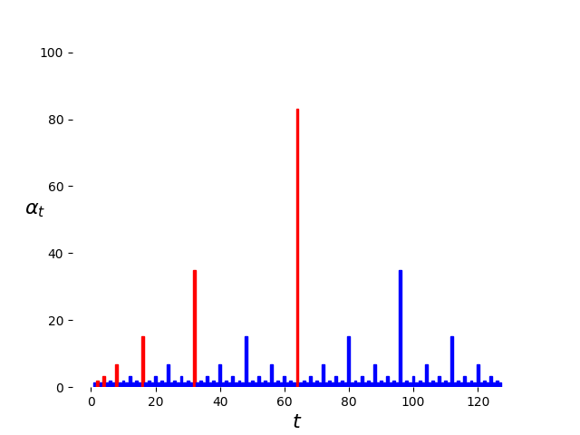
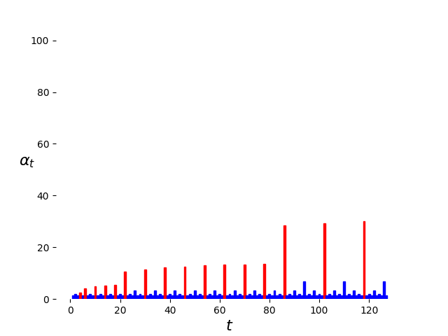
Figure 1: Left: the first 128 steps of the silver stepsize schedule; Right: the first 128 steps of our stepsize schedule (with parameter $c$ adjusted for better illustration). The red bars indicate the positions of the join steps. The number of join steps in the first $t$ steps of the silver stepsize schedule is $\left\lfloor\log_{2}t\right\rfloor$, whereas in our schedule, this number is roughly $\Omega(t^{7/8})$.

Controlling the norm of gradients.

While the above-mentioned concatenation strategy guarantees fast convergence at each join step, we still need to examine the convergence properties at intermediate steps (i.e., the ones between two adjacent join steps). Consider, for concreteness, iteration $\ell$, and denote by $n_{\ell}$ the closest join iteration below $\ell$; see Figure 2 for an illustration. A common strategy to bound the difference $f_{\ell}-f_{n_{\ell}}$ of the associated objective values is to control the norm of the weighted gradients $\alpha_{i}^{2}\|\bm{g}_{i}\|^{2}$ for every $i\in[n_{\ell},\ell]$, which arises from the smoothness and convexity of $f$. A key part of our analysis thus boils down to bounding each $\alpha^{2}_{i}\|\bm{g}_{i}\|^{2}$ using the corresponding weighted gradient at the join step $n_{\ell}$, for which the silver stepsize schedule enjoys some favorable property that enables effective control of $\alpha^{2}_{i}\|\bm{g}_{i}\|^{2}$ in this manner.

Figure 2: An illustration of our analysis strategy to bound $f_{\ell}-f^{*}$ for an intermediate step $\ell$. Here, the yellow point indicates the initial step, whereas the red points indicate the join steps. Here, $n_{\ell}$ indicates the largest join step below $\ell$.

3.3 Key lemmas

Before proceeding to the proof of our main theorem, we single out a couple of key lemmas concerning the primitive stepsize schedule — and in particular, the silver stepsize schedule — that play an important role in our subsequent analysis.

The first lemma below singles out an important property of a primitive stepsize schedules, to be specified by (18).

Lemma 8.

Suppose $\bm{s}=\bm{\alpha}_{1:k-1}$ is a primitive stepsize schedule. Then for any fixed $\bm{x}_{0}$ with gradient $\bm{g}_{0}$, it holds that

$$A_{k}(f_{k}-f_{0})+\frac{1}{2}\|\bm{x}_{k}-\bm{x}_{0}\|^{2}+C_{k}\|\bm{g}_{k}\|^{2}\leq\frac{1}{2}\|\bm{x}_{1}-\bm{x}_{0}\|^{2}+\sum_{i=1}^{k-1}\alpha_{i}\langle\bm{g}_{i},\bm{g}_{0}\rangle-\frac{A_{k}}{2}\|\bm{g}_{0}\|^{2}.$$ (18)

Proof.

From Definition 2 of the primitive stepsize schedule, we obtain

$$A_{k}(f_{k}-f^{*})+C_{k}\|\bm{g}_{k}\|^{2}+\frac{1}{2}\|\bm{x}_{k}-\bm{x}^{*}\|^{2}$$

$$\leq\quad\frac{1}{2}\|\bm{x}_{1}-\bm{x}^{*}\|^{2}+\sum_{i=1}^{k-1}\alpha_{i}\left(f_{i}-f^{*}-\left\langle\bm{g}_{i},\bm{x}_{i}-\bm{x}^{*}\right\rangle+\frac{1}{2}\|\bm{g}_{i}\|^{2}\right).$$ (19)

Also, the basic properties about smooth convex functions (cf. (8)) give

$$\sum_{i=1}^{k-1}\alpha_{i}\left(f_{i}-f_{0}-\left\langle\bm{g}_{i},\bm{x}_{i}-\bm{x}_{0}\right\rangle+\frac{1}{2}\|\bm{g}_{i}-\bm{g}_{0}\|^{2}\right)\leq 0,$$ (20)

which further implies that

$$\sum_{i=1}^{k-1}\alpha_{i}\left(f_{i}-f^{*}-\left\langle\bm{g}_{i},\bm{x}_{i}-\bm{x}^{*}\right\rangle+\frac{1}{2}\|\bm{g}_{i}\|^{2}\right)$$

$$\leq\sum_{i=1}^{k-1}\alpha_{i}\left(f_{i}-f^{*}-\left\langle\bm{g}_{i},\bm{x}_{i}-\bm{x}^{*}\right\rangle+\frac{1}{2}\|\bm{g}_{i}\|^{2}\right)-\sum_{i=1}^{k-1}\alpha_{i}\left(f_{i}-f_{0}-\left\langle\bm{g}_{i},\bm{x}_{i}-\bm{x}_{0}\right\rangle+\frac{1}{2}\|\bm{g}_{i}-\bm{g}_{0}\|^{2}\right)$$

$$=\sum_{i=1}^{k-1}\alpha_{i}\left(f_{0}-f^{*}-\left\langle\bm{g}_{i},\bm{x}_{0}-\bm{x}^{*}\right\rangle+\left\langle\bm{g}_{i},\bm{g}_{0}\right\rangle-\frac{1}{2}\|\bm{g}_{0}\|^{2}\right).$$ (21)

Substituting (21) into (19) and using the fact that $\sum_{i=1}^{k-1}\alpha_{i}\bm{g}_{i}=\bm{x}_{1}-\bm{x}_{k}$, we can derive

$$A_{k}(f_{k}-f^{*})+C_{k}\|\bm{g}_{k}\|^{2}+\frac{1}{2}\|\bm{x}_{k}-\bm{x}^{*}\|^{2}$$

$$\leq\frac{1}{2}\|\bm{x}_{1}-\bm{x}^{*}\|^{2}+\sum_{i=1}^{k-1}\alpha_{i}\left(f_{0}-f^{*}-\left\langle\bm{g}_{i},\bm{x}_{0}-\bm{x}^{*}\right\rangle+\left\langle\bm{g}_{i},\bm{g}_{0}\right\rangle-\frac{1}{2}\|\bm{g}_{0}\|^{2}\right)$$

$$=\frac{1}{2}\|\bm{x}_{1}-\bm{x}^{*}\|^{2}+A_{k}(f_{0}-f^{*})-\sum_{i=1}^{k-1}\alpha_{i}\left\langle\bm{g}_{i},\bm{x}_{0}-\bm{x}^{*}\right\rangle+\sum_{i=1}^{k-1}\alpha_{i}\left\langle\bm{g}_{i},\bm{g}_{0}\right\rangle-\frac{A_{k}}{2}\|\bm{g}_{0}\|^{2}$$

$$=\frac{1}{2}\|\bm{x}_{1}-\bm{x}^{*}\|^{2}+A_{k}(f_{0}-f^{*})-\left\langle\bm{x}_{1}-\bm{x}_{k},\bm{x}_{0}-\bm{x}^{*}\right\rangle+\sum_{i=1}^{k-1}\alpha_{i}\left\langle\bm{g}_{i},\bm{g}_{0}\right\rangle-\frac{A_{k}}{2}\|\bm{g}_{0}\|^{2}.$$ (22)

To continue, we make the observation that

$$\frac{1}{2}\|\bm{x}_{1}-\bm{x}^{*}\|^{2}-\frac{1}{2}\|\bm{x}_{k}-\bm{x}^{*}\|^{2}-\left\langle\bm{x}_{1}-\bm{x}_{k},\bm{x}_{0}-\bm{x}^{*}\right\rangle =\frac{1}{2}\|\bm{x}_{1}\|^{2}-\frac{1}{2}\|\bm{x}_{k}\|^{2}-\left\langle\bm{x}_{1},\bm{x}_{0}\right\rangle+\left\langle\bm{x}_{k},\bm{x}_{0}\right\rangle$$

$$=\frac{1}{2}\|\bm{x}_{1}-\bm{x}_{0}\|^{2}-\frac{1}{2}\|\bm{x}_{k}-\bm{x}_{0}\|^{2},$$

which combined with (22) yields

$$A_{k}(f_{k}-f_{0})+C_{k}\|\bm{g}_{k}\|^{2}+\frac{1}{2}\|\bm{x}_{k}-\bm{x}^{*}\|^{2}\leq\frac{1}{2}\|\bm{x}_{1}-\bm{x}_{0}\|^{2}+\sum_{i=1}^{k-1}\alpha_{i}\left\langle\bm{g}_{i},\bm{g}_{0}\right\rangle-\frac{A_{k}}{2}\|\bm{g}_{0}\|^{2}$$

as claimed. ∎

Furthermore, the result in Lemma 8 allows us to control the gradient norm at the last step, provided that a primitive stepsize schedule is adopted.

Lemma 9.

Assume $\bm{s}=\bm{\alpha}_{1:k-1}$ is a primitive stepsize schedule. Assume $\bm{x}_{1}=\bm{x}_{0}-\alpha_{0}\bm{g}_{0}$. Then one has

$$C_{k}\|\bm{g}_{k}\|^{2}\leq\left(\frac{\alpha_{0}^{2}}{2}+\frac{(A_{k}+1)^{2}}{2}-\alpha_{0}-\frac{A_{k}}{2}\right)\|\bm{g}_{0}\|^{2}.$$ (23)

Proof.

Because $\bm{\alpha}_{1:k-1}$ is a primitive stepsize schedule, it follows from Lemma 8 that

$$A_{k}(f_{k}-f_{0})+\frac{1}{2}\|\bm{x}_{k}-\bm{x}_{0}\|^{2}+C_{k}\|\bm{g}_{k}\|^{2}\leq\frac{1}{2}\|\bm{x}_{1}-\bm{x}_{0}\|^{2}+\sum_{i=1}^{k-1}\alpha_{i}\left\langle\bm{g}_{i},\bm{g}_{0}\right\rangle-\frac{A_{k}}{2}\|\bm{g}_{0}\|^{2}.$$

We also make note of the following basic facts:

$$\bm{x}_{1} =\bm{x}_{0}-\alpha_{0}\bm{g}_{0};$$ (24a)

$$\sum_{i=1}^{k-1}\alpha_{i}\bm{g}_{i} =\bm{x}_{1}-\bm{x}_{k}=\bm{x}_{0}-\bm{x}_{k}-\alpha_{0}\bm{g}_{0};$$ (24b)

$$f_{0}-f_{k} \leq\left\langle\bm{g}_{0},\bm{x}_{0}-\bm{x}_{k}\right\rangle-\frac{1}{2}\|\bm{g}_{0}-\bm{g}_{k}\|^{2};$$ (24c)

$$(A_{k}+1)\left\langle\bm{g}_{0},\bm{x}_{0}-\bm{x}_{k}\right\rangle \leq\frac{1}{2}\|\bm{x}_{k}-\bm{x}_{0}\|^{2}+\frac{(A_{k}+1)^{2}}{2}\|\bm{g}_{0}\|^{2}.$$ (24d)

Putting the above inequalities together, we arrive at

$$C_{k}\|\bm{g}_{k}\|^{2}\leq\left(\frac{\alpha_{0}^{2}}{2}+\frac{(A_{k}+1)^{2}}{2}-\alpha_{0}-\frac{A_{k}}{2}\right)\|\bm{g}_{0}\|^{2}$$ (25)

as claimed. ∎

Additionally, the following lemma enables effective control of the gradient norms in all intermediate steps.

Lemma 10.

Fix $i\geq 1$ and $\alpha\geq 0$, and let $k=2^{i}$. Denote by $\overline{\bm{s}}_{i}=[\alpha_{1},\dots,\alpha_{k-1}]^{\top}$ the first $k-1$ stepsizes of the $i$-th order silver stepsize schedule $\overline{\bm{s}}_{i}$. Fix $\bm{x}_{0}$, set $\alpha_{0}=\alpha$, and let $\bm{x}_{1}=\bm{x}_{0}-\alpha_{0}\bm{g}_{0}$. If $\alpha\geq\max\{(\sqrt{2}-1)A_{k},1\}$, then one has

$$\alpha_{\ell}^{2}\|\bm{g}_{\ell}\|^{2} \leq 16^{i}\alpha^{2}\|\bm{g}_{0}\|^{2}$$ (26a)

$$f_{\ell}-f_{0} \leq\frac{3}{2}\cdot(32^{i}\alpha^{2}\|\bm{g}_{0}\|^{2})$$ (26b)

for any $1\leq\ell\leq k-1$.

Proof.

We shall prove the first claim of this lemma by induction. Regarding the base case with $i=1$, from the fact that $\bm{x}_{1}=\bm{x}_{0}-\alpha\bm{g}_{0}$ and $\alpha_{1}=\sqrt{2}$. The convexity and 1-smoothness of $f$ give

$$\|\bm{g}_{1}-\bm{g}_{0}\|^{2}\leq\langle\bm{g}_{0}-\bm{g}_{1},\bm{x}_{0}-\bm{x}_{1}\rangle=\alpha\langle\bm{g}_{0}-\bm{g}_{1},\bm{g}_{0}\rangle.$$

Rearrange terms to yield

$$\|\bm{g}_{1}\|^{2} \leq(\alpha-1)\|\bm{g}_{0}\|^{2}-(\alpha-2)\langle\bm{g}_{0},\bm{g}_{1}\rangle\leq(\alpha-1)\|\bm{g}_{0}\|^{2}+\frac{(\alpha-2)^{2}}{2}\|\bm{g}_{0}\|^{2}+\frac{1}{2}\|\bm{g}_{1}\|^{2}$$

$$\qquad\Longrightarrow\qquad\|\bm{g}_{1}\|^{2}\leq\big{(}(\alpha-2)^{2}+2\alpha-2\big{)}\|\bm{g}_{0}\|^{2}\leq 16\alpha^{2}\|\bm{g}_{0}\|^{2}.$$

Next, assume the claim (26a) holds for $i-1$ for some $i\geq 2$, then it suffices to prove it for $\ell\geq 2^{i-1}$. Let $\ell^{*}=2^{i-1}$. Because $\overline{\bm{s}}_{i-1}=\bm{\alpha}_{1:\ell^{*}-1}$ is a primitive stepsize schedule, it follows from Lemma 9 that

$$C_{\ell^{*}}\|\bm{g}_{\ell^{*}}\|^{2}\leq\left(\frac{\alpha^{2}}{2}+\frac{(A_{\ell^{*}}+1)^{2}}{2}-\alpha-\frac{A_{\ell^{*}}}{2}\right)\|\bm{g}_{0}\|^{2}.$$ (27)

Recall that $\alpha_{\ell^{*}}=\varphi(A_{\ell^{*}},A_{\ell^{*}})=(\sqrt{2}-1)A_{\ell^{*}}+\sqrt{2}$ and $A_{\ell^{*}}\geq\sqrt{2}$ (a consequence of Lemma 7). Recognizing that $\frac{\alpha_{\ell^{*}}}{A_{\ell^{*}}}=\frac{(\sqrt{2}-1)A_{\ell^{*}}+\sqrt{2}}{A_{\ell^{*}}}\leq\sqrt{2}$, $C_{\ell^{*}}=\frac{A_{\ell}^{*}(A_{\ell}^{*}+1)}{2}$ and $\alpha\geq\min\{(\sqrt{2}-1)A_{k},1\}$, we can deduce that

$$\alpha^{2}_{\ell^{*}}\|\bm{g}_{\ell^{*}}\|^{2} =\frac{\alpha_{\ell^{*}}^{2}}{C_{\ell^{*}}}\cdot C_{\ell^{*}}\|\bm{g}_{\ell^{*}}\|^{2}$$

$$\leq 2\frac{\alpha^{2}_{\ell^{*}}}{A_{\ell^{*}}(A_{\ell^{*}}+1)}\cdot\left(\frac{1}{2}+\frac{A_{\ell^{*}}^{2}+A_{\ell^{*}}}{2\alpha^{2}}\right)\alpha^{2}\|\bm{g}_{0}\|^{2}$$

$$\leq\left(2+\frac{\alpha_{\ell^{*}}^{2}}{\alpha^{2}}\right)\alpha^{2}\|\bm{g}_{0}\|^{2}$$ (28)

$$=\left(2+\frac{\alpha_{\ell^{*}}^{2}}{A_{\ell^{*}}^{2}}\cdot\frac{A_{\ell^{*}}^{2}}{\alpha^{2}}\right)\alpha^{2}\|\bm{g}_{0}\|^{2}$$

$$\leq\big{(}2+(2+\sqrt{2})^{2}\big{)}\alpha^{2}\|\bm{g}_{0}\|^{2}$$

$$\leq 16\alpha^{2}\|\bm{g}_{0}\|^{2}.$$

Applying induction over the $(i-1)$-th order silver stepsize schedule $\bm{\alpha}_{2^{i-1}+1:2^{i}-1}$ with $\alpha=\alpha_{2^{i-1}}=(\sqrt{2}-1)A_{\ell^{*}}+\sqrt{2}\geq\min\{(\sqrt{2}-1)A_{\ell^{*}},1\}$, we can show that

$$\alpha_{\ell}^{2}\bm{g}_{\ell}^{2}\leq 16^{i-1}\alpha_{\ell^{*}}^{2}\|\bm{g}_{\ell^{*}}\|^{2}\leq 16^{i}\alpha^{2}\|\bm{g}_{0}\|^{2},\qquad\ell\in[2^{i-1},2^{i}-1].$$ (29)

We now turn to the second claim of this lemma. From (8f) and the fact that each stepsize in $\overline{\bm{s}}_{i}$ is at least $1$ for all $i\geq 1$ — which holds since $\varphi(x,y)>1$ for all $x,y\geq 0$ — we see that

$$f_{\ell}-f_{0} =\sum_{j=0}^{\ell-1}(f_{j+1}-f_{j})\leq\sum_{j=0}^{\ell-1}\frac{\alpha_{j}^{2}+2\alpha_{j}}{2}\|\bm{g}_{i}\|^{2}$$

$$\leq\frac{3}{2}\left(\sum_{j=0}^{\ell-1}\alpha_{i}^{2}\|\bm{g}_{i}\|^{2}\right)\leq\frac{3}{2}\cdot\big{(}32^{i}\alpha^{2}\|\bm{g}_{0}\|^{2}\big{)},$$

which concludes the proof. ∎

3.4 Proof of Theorem 1

We are now positioned to prove our main result in Theorem 1, based on the stepsize schedule $\widehat{\bm{s}}=[\alpha_{i}]_{i=1}^{\infty}$ constructed in Section 3.1. Let us remind the readers of several notation below.

• $t_{i}$: the length of the $i$-th subsequence $\widehat{\bm{s}}_{i}=[\alpha_{1},\dots,\alpha_{t_{i}}]^{\top}$ (see Section 3.1), corresponding to the first $t_{i}$ stepsizes in $\widehat{\bm{s}}$. .

• $o_{t}$: the integer such that $\sum_{j=1}^{o_{t}-1}k_{j}2^{j}<t\leq\sum_{j=1}^{o_{t}}k_{j}2^{j}$. Clearly, the length of the $(i+1)$-th subsequence (including the $(t_{i}+1)$-th step) is $2^{o_{t_{i}+1}}$, and $t_{i+1}=t_{i}+2^{o_{t_{i}+1}}$.

• $A_{t}$ and $C_{t}$: $A_{t}=\sum_{i=1}^{t-1}\alpha_{i}$ and $C_{t}=\frac{A_{t}(A_{t}+1)}{2}$, where we suppress the dependency on $\widehat{\bm{s}}$ for notational convenience.

• $\alpha_{j}(\overline{s}_{i})$: the $j$-th stepsize in the sequence $\overline{\bm{s}}_{i}$.

It is also worth noting that Lemma 7 gives

$$2^{o_{t_{i}+1}}\leq 2\cdot 2^{o_{t_{i}}}\leq 4t_{i}^{\frac{1}{c+1}}.$$ (30)

Consider any $i\geq 1$. In view of Lemma 4, we know that $\widehat{\bm{s}}_{i}$ is primitive. Given that $\{\bm{x}_{j}\}_{j=1}^{t_{i}+1}$ is the GD trajectory with stepsize schedule $\widehat{\bm{s}}_{i}$, we see from Definition 2 of the primitive stepsize schedule that

$$A_{t_{i}+1}(f_{t_{i}+1}-f^{*})+C_{t_{i}+1}\|\bm{g}_{t_{i}+1}\|^{2}+\frac{1}{2}\|\bm{x}_{t_{i}+1}-\bm{x}^{*}\|^{2}\leq\frac{1}{2}\|\bm{x}_{1}-\bm{x}^{*}\|^{2},$$

which immediately implies that

$$f_{t_{i}+1}-f^{*} \leq\frac{\|\bm{x}_{1}-\bm{x}^{*}\|^{2}}{A_{t_{i}+1}};$$ (31a)

$$\|\bm{g}_{t_{i}+1}\|^{2} \leq\frac{\|\bm{x}_{1}-\bm{x}^{*}\|^{2}}{2C_{t_{i}+1}}\leq\frac{\|\bm{x}_{1}-\bm{x}^{*}\|^{2}}{A_{t_{i}+1}^{2}}.$$ (31b)

Additionally, by construction we have $\alpha_{t_{i}+1}=\varphi(x,y)$ due to the concatenation operation, where

$$x =\sum_{j=1}^{t_{i}}\alpha_{j}\geq\frac{1}{36}t_{i}^{\frac{c+\log_{2}{\rho}}{c+1}}\qquad\qquad\quad\qquad;$$

$$y =\sum_{j=t_{i}+2}^{t_{i+1}}\alpha_{j}=\sum_{j=1}^{2^{o_{t_{i}+1}}-1}\alpha_{j}(\overline{\bm{s}}_{o_{t_{i}+1}})=\rho^{o_{t_{i}+1}}-1\leq 2\cdot t_{i}^{\frac{\log_{2}{\rho}}{c+1}}.$$

Here, both of the inequalities above arise from Lemma 7. It is also easy to observe that $x\geq y$. It then follows that

$$\alpha_{t_{i}+1}=\varphi(x,y) =\frac{-(x+y)+\sqrt{(x+y+2)^{2}+4(x+1)(y+1)}}{2}$$

$$=\frac{4(xy+2x+2y+2)}{2(x+y+\sqrt{(x+y+2)^{2}+4(x+1)(y+1)})}$$

$$\leq\frac{xy+2x+2y+2}{x+y+2}$$

$$\leq y+2$$

$$=\rho^{o_{t_{i}+1}}+1.$$

Moreover, recognizing that

$$\frac{\partial\varphi(x,y)}{\partial x}=\frac{1}{2}\left(-1+\frac{x+3y+4}{\sqrt{x^{2}+(6y+8)x+8y+8}}\right)\geq 0$$

for all $(x,y)\geq 0$, we immediately obtain

$$\alpha_{t_{i}+1}=\varphi(x,y) \geq\varphi(y,y)=(\sqrt{2}-1)y+\sqrt{2}.$$

Invoking (31b) and Lemma 10 over the $(i+1)$-th sub-sequence with $\alpha=\alpha_{t_{i}+1}\geq(\sqrt{2}-1)y+\sqrt{2}$, we can show that: for any $\ell$ obeying $t_{i}+1<\ell\leq t_{i+1}$,

$$f_{\ell}-f_{t_{i}+1} \overset{\mathrm{(i)}}{\leq}\frac{3}{2}\cdot(\ell-t_{i}-1)\cdot O\left(\max_{t_{i}+1\leq j\leq\ell}\alpha_{j}^{2}\|\bm{g}_{j}\|^{2}\right)$$

$$\overset{\mathrm{(ii)}}{\leq}2^{o_{t_{i}+1}}\cdot O\left(16^{o_{t_{i}+1}}\alpha_{t_{i}+1}^{2}\|\bm{g}_{t_{i}+1}\|^{2}\right)$$

$$\overset{\mathrm{(iii)}}{\leq}O\left(32^{o_{t_{i}+1}}\frac{\alpha_{t_{i}+1}^{2}}{A^{2}_{t_{i}+1}}\|\bm{x}_{1}-\bm{x}^{*}\|^{2}\right)$$

$$\overset{\mathrm{(iv)}}{\leq}O\left(\frac{\|\bm{x}_{1}-\bm{x}^{*}\|^{2}\cdot t_{i}^{\frac{5+2\log_{2}\rho}{c+1}}}{t_{i}^{\frac{2(c+\log_{2}\rho)}{c+1}}}\right)$$

$$=O\left(\frac{\|\bm{x}_{1}-\bm{x}^{*}\|^{2}}{\ell^{\frac{2(c+\log_{2}\rho)-5-2\log_{2}\rho}{c+1}}}\right)$$

$$\leq O\left(\frac{\|\bm{x}_{1}-\bm{x}^{*}\|^{2}}{\ell^{\frac{c+\log_{2}\rho}{c+1}}}\right).$$

Here, (i) is valid since, according to (8f) and the fact that $\alpha_{j}\geq 1$ (as $\varphi(x^{\prime},y^{\prime})\geq 1$ for any $x^{\prime},y^{\prime}>0$),

$$f_{\ell}-f_{t_{i}+1}=\sum_{j=t_{i}+1}^{\ell-1}\big{(}f_{j+1}-f_{j}\big{)}\leq\sum_{j=t_{i}+1}^{\ell-1}\frac{\alpha_{j}^{2}+2\alpha_{j}}{2}\|\bm{g}_{j}\|^{2}\leq\sum_{j=t_{i}+1}^{\ell-1}\frac{3\alpha_{j}^{2}}{2}\|\bm{g}_{j}\|^{2};$$

(ii) arises from Lemma 10; (iii) is a consequence of (31b); and (iv) invokes Lemma 7, inequality (30), as well as the property that $\alpha_{t_{i}+1}\leq\rho^{o_{t_{i}+1}}+3=O(\rho^{o_{t_{i}+1}})$. This taken together with (31a) further results in

$$f_{\ell}-f^{*} =f_{\ell}-f_{t_{i}+1}+\big{(}f_{t_{i}+1}-f^{*}\big{)}$$

$$\leq O\left(\frac{\|\bm{x}_{1}-\bm{x}^{*}\|^{2}}{\ell^{\frac{c+\log_{2}\rho}{c+1}}}+\frac{\|\bm{x}_{1}-\bm{x}^{*}\|^{2}}{A_{t_{i}+1}}\right)=O\left(\frac{\|\bm{x}_{1}-\bm{x}^{*}\|^{2}}{\ell^{\frac{c+\log_{2}\rho}{c+1}}}\right).$$

Consequently, we have shown that, for any $\ell\in\cup_{i\geq 1}(t_{i},t_{i+1}]=[3,\infty)$,

$$f_{\ell}-f^{*}\leq O\left(\frac{\|\bm{x}_{1}-\bm{x}^{*}\|^{2}}{A_{t_{i}+1}}+\frac{\|\bm{x}_{1}-\bm{x}^{*}\|^{2}}{\ell^{\frac{c+\log_{2}\rho}{c+1}}}\right)=O\left(\frac{\|\bm{x}_{1}-\bm{x}^{*}\|^{2}}{\ell^{\frac{c+\log_{2}\rho}{c+1}}}\right).$$

When $\ell<3$, it is easily seen that

$$f_{1}-f^{*} \leq\frac{\|\bm{x}_{1}-\bm{x}^{*}\|^{2}}{2}\qquad\text{and}$$

$$f_{2}-f^{*} \leq f_{1}-f^{*}+\frac{\alpha_{1}^{2}+2\alpha_{1}}{2}\|\bm{g}_{1}\|^{2}\leq(1+\alpha_{1}^{2}+2\alpha_{1})(f_{1}-f^{*})\leq\frac{9\|\bm{x}_{1}-\bm{x}^{*}\|^{2}}{2},$$

where we have made use of (8f). We have thus completed the proof by recalling that $c=7$.

4 Extension to smooth and strongly convex problems

In this section, we further extend our result to accommodate smooth and strongly convex optimization; that is, we assume that the objective function $f$ in (1) is $1$-smooth and $\mu$-strongly convex for some strong convexity parameter $\mu\in(0,1]$. Here and throughout, we denote by $\kappa=1/\mu$ the condition number. Our result, which guarantees acceleration of standard GD theory (i.e., $\exp(-\Theta(T/\kappa))$ in an anytime manner, is stated as follows.

Theorem 11.

There is a stepsize schedule $\{\alpha_{t}\}_{t=1}^{\infty}$, generated without knowing the stopping time, such that the gradient descent iterates (2) obey

$$f(\bm{x}_{T})-f^{*}\leq O\left(\exp\left(-\frac{CT}{\kappa^{\varsigma}}\right)\|\bm{x}_{1}-\bm{x}^{*}\|^{2}\right),$$ (32)

where $\varsigma=1/\vartheta=\frac{8}{7+\log_{2}\rho}<0.97$, and $C>0$ is some numerical constant. Here, $T$ denotes an arbitrary stopping time that is unknown a priori.

Proof of Theorem 11.

Recall our construction of $\widehat{\bm{s}}$ in the proof of Theorem 1 (see Section 3.1). According to Theorem 1, there exists a universal constant $C_{0}>0$ such that running GD with the stepsize schedule $\widehat{\bm{s}}$ achieves

$$f(\bm{x}_{t})-f^{*}\leq\frac{C_{0}\|\bm{x}_{1}-\bm{x}^{*}\|^{2}}{t^{\vartheta}}.$$

Let us begin by constructing a stepsize schedule tailored to the $\mu$-strongly convex problem. Take $\tau=\tau(\mu)$ to be the smallest integer such that $A_{\tau+1}(\widehat{\bm{s}})\geq\frac{4C_{0}}{\mu}=4C_{0}\kappa$. Lemma 7 tells us that

$$\frac{1}{36}\tau^{\vartheta}=\frac{1}{36}\tau^{\frac{c+\log_{2}\rho}{c+1}}\leq A_{\tau}(\widehat{\bm{s}})\leq 4C_{0}\kappa,$$ (33)

which implies that

$$\tau\leq 144C_{0}\kappa^{\frac{1}{\vartheta}}=144C_{0}\kappa^{\varsigma}.$$

Now, let $\widetilde{\bm{s}}=\bm{\alpha}_{1:\tau}(\widehat{\bm{s}})$ (i.e., the first $\tau$ stepsizes in $\widehat{\bm{s}}$), and set $\widetilde{\bm{s}}^{*}$ to be the infinite stepsize schedule $[\widetilde{\bm{s}}^{\top},\widetilde{\bm{s}}^{\top},\ldots]^{\top}$; that is, $\alpha_{i\tau+j}(\widetilde{\bm{s}}^{*})=\alpha_{j}(\widetilde{\bm{s}})=\alpha_{j}(\widehat{\bm{s}})$ for any $i\geq 0$ and $1\leq j\leq\tau$.

Next, we would like to show that the claimed result (32) holds with the stepsize schedule $\widehat{\bm{s}}^{*}$. In view of Theorem 1, we know that

$$f_{j}-f^{*} \leq\frac{C_{0}\|\bm{x}_{1}-\bm{x}^{*}\|^{2}}{j^{\vartheta}}\leq 55C_{0}\exp\left(-\frac{j}{36C_{0}\kappa^{\varsigma}}\right)\cdot\|\bm{x}_{1}-\bm{x}^{*}\|^{2}\qquad\text{for all }1\leq j\leq\tau;$$ (34)

$$f_{\tau+1}-f^{*} \leq\frac{C_{0}\|\bm{x}_{1}-\bm{x}^{*}\|^{2}}{\tau^{\theta}}=\frac{\|\bm{x}_{1}-\bm{x}^{*}\|^{2}}{144\kappa^{\varsigma\cdot\vartheta}}=\frac{\|\bm{x}_{1}-\bm{x}^{*}\|^{2}}{144\kappa}=\frac{\mu\|\bm{x}_{1}-\bm{x}^{*}\|^{2}}{144},$$ (35)

where we have invoked (33). Observing that $f_{\tau+1}-f^{*}\geq\frac{\mu\|\bm{x}_{\tau+1}-\bm{x}^{*}\|^{2}}{2}$ due to $\mu$-strong convexity, we have

$$\|\bm{x}_{\tau+1}-\bm{x}^{*}\|^{2}\leq\frac{1}{72}\|\bm{x}_{1}-\bm{x}^{*}\|^{2}.$$

Invoking similar arguments reveals that: for any $i\geq 1$ and $1\leq j\leq\tau$, one has

$$\frac{\mu}{2}\|\bm{x}_{i\tau+1}-\bm{x}^{*}\|^{2}\leq f_{i\tau+1}-f^{*}\leq\frac{\mu\|\bm{x}_{(i-1)\tau+1}-\bm{x}^{*}\|^{2}}{4}$$

$$\text{and}\qquad f_{i\tau+j}-f^{*}\leq\frac{C_{0}\|\bm{x}_{i\tau+1}-\bm{x}^{*}\|^{2}}{j^{\vartheta}}\leq C_{0}\|\bm{x}_{i\tau+1}-\bm{x}^{*}\|^{2}.$$

As a result, we can deduce that

$$\|\bm{x}_{i\tau+1}-\bm{x}^{*}\|^{2} \leq\frac{1}{2}\|\bm{x}_{(i-1)\tau+1}-\bm{x}^{*}\|^{2}$$

$$\leq\left(\frac{1}{2}\right)^{i}\|\bm{x}_{1}-\bm{x}^{*}\|^{2}$$

$$\leq\exp\left(-\log 2\cdot\frac{i\tau+1}{2\tau}\right)\|\bm{x}_{1}-\bm{x}^{*}\|^{2}$$

$$\leq\exp\left(-\frac{i\tau+1}{576C_{0}\kappa^{\varsigma}}\right)\|\bm{x}_{1}-\bm{x}^{*}\|^{2},$$

and as a result,

$$f_{i\tau+j}-f^{*}\leq C_{0}\|\bm{x}_{i\tau+1}-\bm{x}^{*}\|^{2}\leq C_{0}\exp\left(-\frac{i\tau+1}{576C_{0}\kappa^{\varsigma}}\right)\|\bm{x}_{1}-\bm{x}^{*}\|^{2}\leq C_{0}\exp\left(-\frac{i\tau+j}{1152C_{0}\kappa^{\varsigma}}\right)\|\bm{x}_{1}-\bm{x}^{*}\|^{2}.$$ (36)

To finish up, combine (34) and (36) to arrive at

$$f_{T}-f^{*}\leq 55C_{0}\exp\left(-\frac{CT}{\kappa^{\varsigma}}\right)\cdot\|\bm{x}_{1}-\bm{x}^{*}\|^{2}\qquad\text{for any }T\geq 1,$$

where $C=\frac{1}{1152C_{0}}$. This concludes the proof. ∎

Appendix A Proof of Lemma 7

First, let us look at the case with $o_{t}=1$, for which we have $t\leq 2k_{1}=2^{c+1}$. Given that $\varphi(x,y)>1$ for all $x,y\geq 0$, we can easily verify that

$$A_{t+1}(\widehat{\bm{s}})\geq t\geq\frac{1}{36}t^{\frac{c+\log_{2}\rho}{c+1}}.$$

It is also easily seen that $2^{o_{t}}=2\leq 2t^{\frac{1}{c+1}}.$

Now, let us turn to the case where $o_{t}\geq 2$. Let $m\in[1,k_{o_{t}}]$ be the integer such that $\sum_{j=1}^{o_{t}-1}k_{j}2^{j}+(m-1)\cdot 2^{o_{t}}<t\leq\sum_{j=1}^{o_{t}-1}k_{j}2^{j}+m\cdot 2^{o_{t}}$. By definition, we have

$$t \leq\sum_{j=1}^{o_{t}-1}k_{j}2^{j}+m2^{o_{t}}\leq 2\cdot 2^{(c+1)(o_{t}-1)}+m2^{o_{t}};$$

$$A_{t+1}(\widehat{\bm{s}}) \geq\sum_{j=1}^{o_{t}-1}(\rho^{j}-1)\cdot k_{j}+(m-1)(\rho^{o_{t}}-1)\geq\frac{1}{2}\cdot 2^{(c+\log_{2}\rho)(o_{t}-1)}+\frac{m-1}{2}\rho^{o_{t}},$$

where the second line invokes Lemma 6.

• If $m2^{o_{t}}\leq 2^{(c+1)(o_{t}-1)}$, then we have $t\leq 3\cdot 2^{(c+1)(o_{t}-1)}$, which means that $A_{t+1}(\widehat{\bm{s}})\geq\frac{1}{2}\cdot 2^{(c+\log_{2}\rho)(o_{t}-1)}\geq\frac{1}{18}t^{\frac{c+\log_{2}\rho}{c+1}}$.

• If $m2^{o_{t}}>2^{(c+1)(o_{t}-1)}$ — i.e, $2^{o_{t}c}\geq m>2^{o_{t}c-c-1}\geq 1$ — then one has

  $$t^{\frac{c+\log_{2}\rho}{c+1}}<9(m2^{o_{t}})^{\frac{c+\log_{2}\rho}{c+1}}\leq 9\cdot m\rho^{o_{t}}\leq 36\cdot\frac{m-1}{2}\rho^{o_{t}}\leq 36A_{t+1}(\widehat{\bm{s}}).$$

Putting these two cases together establishes the claim (16).

Regarding the second claim, in the case where $o_{t}\geq 2$, we have

$$t\geq\sum_{j=1}^{o_{t}-1}k_{j}2^{j}=\sum_{j=1}^{o_{t}-1}2^{(c+1)j}\geq 2^{(c+1)(o_{t}-1)},$$ (37)

thus indicating that $2t^{\frac{1}{c+1}}\geq 2^{o_{t}}$.

Appendix B Proof of preliminary facts from Zhang and Jiang, (2024)

B.1 Proof of Lemma 3

As mentioned previously, this lemma was established by Zhang and Jiang, (2024). We present the proof for completeness.

To begin with, we single out the following lemma, originally established by Zhang and Jiang, (2024, Lemma 3.1), that plays a key role in the proof of Lemma 3. We shall provide a proof in Appendix B.2.

Lemma 12.

(Zhang and Jiang, (2024, Lemma 3.1)) Assume that $\bm{\alpha}_{1:\ell-1}$ is primitive. For any $\alpha\in[1,A_{\ell}+2)$, if we set $\alpha_{0}=\alpha$, then it holds that

$$f_{0}-f_{\ell}\geq\frac{A_{\ell}+3\alpha-2\alpha^{2}}{2(A_{\ell}+2-\alpha)}\|\bm{g}_{0}\|^{2}+\frac{2A_{\ell}^{2}+3A_{\ell}+\alpha}{2(A_{\ell}+2-\alpha)}\|\bm{g}_{\ell}\|^{2}.$$

Next, in view of the definition of the primitive stepsize schedule (cf. Definition 2), we can easily see that

$$x(f_{\ell}-f^{*})+\frac{x(x+1)}{2}\|\bm{g}_{\ell}\|^{2}+\frac{1}{2}\|\bm{x}_{\ell}-\bm{x}^{*}\|^{2} \leq\frac{1}{2}\|\bm{x}_{1}-\bm{x}^{*}\|^{2}+\sum_{i=1}^{\ell-1}\alpha_{i}\left(f_{i}-f^{*}-\langle\bm{g}_{i},\bm{x}_{i}-\bm{x}^{*}\rangle+\frac{1}{2}\|\bm{g}_{i}\|^{2}\right),$$

$$y(f_{k}-f^{*})+\frac{y(y+1)}{2}\|\bm{g}_{k}\|^{2}+\frac{1}{2}\|\bm{x}_{k}-\bm{x}^{*}\|^{2} \leq\frac{1}{2}\|\bm{x}_{\ell+1}-\bm{x}^{*}\|^{2}+\sum_{i=\ell+1}^{k-1}\alpha_{i}\left(f_{i}-f^{*}-\langle\bm{g}_{i},\bm{x}_{i}-\bm{x}^{*}\rangle+\frac{1}{2}\|\bm{g}_{i}\|^{2}\right),$$

where we take $x=A_{\ell}$ and $y=A_{k}-A_{\ell+1}$ for notational simplicity. Given that

$$z\coloneqq x+y+\alpha=A_{\ell}+(A_{k}-A_{\ell+1})+\alpha_{\ell}=A_{k},$$

Lemma 12 tells us that

$$(x+\alpha)(f_{k}-f_{\ell})\leq-\frac{(x+\alpha)(y+3\alpha-2\alpha^{2})}{2(y+2-\alpha)}\|\bm{g}_{\ell}\|^{2}-\frac{(x+\alpha)(2y^{2}+3y+\alpha)}{2(y+2-\alpha)}\|\bm{g}_{k}\|^{2}.$$ (38)

Adding the above three inequalities and utilizing $z=x+y+\alpha$ yield

$$L_{1}+L_{2}+L_{3}+L_{4}\leq R_{1}+R_{2}+R_{3}+R_{4},$$ (39)

where

$$L_{1} =z(f_{k}-f^{*})+\frac{z(z+1)}{2}\|\bm{g}_{k}\|^{2}+\frac{1}{2}\|\bm{x}_{k}-\bm{x}^{*}\|^{2}=A_{k}(f_{k}-f^{*})+C_{k}\|\bm{g}_{k}\|^{2}+\frac{1}{2}\|\bm{x}_{k}-\bm{x}^{*}\|^{2};$$

$$L_{2} =-\alpha(f_{\ell}-f^{*})+\frac{1}{2}\|\bm{x}_{\ell}-\bm{x}^{*}\|^{2};$$

$$L_{3} =\frac{x(x+1)}{2}\|\bm{g}_{\ell}\|^{2};$$

$$L_{4} =\frac{y(y+1)-z(z+1)}{2}\|\bm{g}_{k}\|^{2};$$

$$R_{1} =\frac{1}{2}\|\bm{x}_{1}-\bm{x}^{*}\|^{2}+\sum_{i=1}^{k-1}\alpha_{i}\bigg{(}f_{i}-f^{*}-\langle\bm{g}_{i},\bm{x}_{i}-\bm{x}^{*}\rangle+\frac{1}{2}\|\bm{g}_{i}\|^{2}\bigg{)};$$

$$R_{2} =\frac{1}{2}\|\bm{x}_{\ell+1}-\bm{x}^{*}\|^{2}-\alpha\big{(}f_{\ell}-f^{*}-\langle\bm{g}_{\ell},\bm{x}_{\ell}-\bm{x}^{*}\rangle\big{)}-\frac{1}{2}\alpha^{2}\|\bm{g}_{\ell}\|^{2};$$

$$R_{3} =\left(-\frac{\alpha}{2}+\frac{\alpha^{2}}{2}-\frac{(x+\alpha)(y+3\alpha-2\alpha^{2})}{(y+2-\alpha)}\right)\|\bm{g}_{\ell}\|^{2};$$

$$R_{4} =-\frac{(x+\alpha)(2y^{2}+3y+\alpha)}{y+2-\alpha}\|\bm{g}_{k}\|^{2}.$$

We now proceed to simplify (39). Firstly, it is readily seen that

$$L_{2}-R_{2} =\frac{1}{2}\|\bm{x}_{\ell}-\bm{x}^{*}\|^{2}-\frac{1}{2}\|\bm{x}_{\ell+1}-\bm{x}^{*}\|^{2}-\alpha\langle\bm{g}_{\ell},\bm{x}_{\ell}-\bm{x}^{*}\rangle+\frac{1}{2}\alpha^{2}\|\bm{g}_{\ell}\|^{2}$$

$$=\frac{1}{2}\|\bm{x}_{\ell}-\bm{x}^{*}\|^{2}-\frac{1}{2}\|\bm{x}_{\ell}-\bm{x}^{*}-\alpha\bm{g}_{\ell}\|^{2}-\alpha\langle\bm{g}_{\ell},\bm{x}_{\ell}-\bm{x}^{*}\rangle+\frac{1}{2}\alpha^{2}\|\bm{g}_{\ell}\|^{2}$$

$$=0.$$

Secondly, recalling our specific choice $\alpha=\varphi(x,y)=\frac{-(x+y)+\sqrt{(x+y+2)^{2}+4(x+1)(y+1)}}{2}$, we can easily verify that

$$\alpha^{2}+(x+y)\alpha-(xy+2x+2y+2)=0.$$

This allows one to demonstrate that

$$L_{3}-R_{3} =\left(\frac{x(x+1)}{2}+\frac{\alpha}{2}-\frac{\alpha^{2}}{2}+\frac{(x+\alpha)(y+3\alpha-2\alpha^{2})}{2(y+2-\alpha)}\right)\|\bm{g}_{\ell}\|^{2}=0;$$

$$L_{4}-R_{4} =\left(\frac{y(y+1)-z(z+1)}{2}+\frac{(x+\alpha)(2y^{2}+3y+\alpha)}{y+2-\alpha}\right)\|\bm{g}_{k}\|^{2}=0.$$

Substitution into (39) then results in $L_{1}\leq R_{1},$ namely,

$$A_{k}(f_{k}-f^{*})+C_{k}\|\bm{g}_{k}\|^{2}+\frac{1}{2}\|\bm{x}_{k}-\bm{x}^{*}\|^{2} \leq\frac{1}{2}\|\bm{x}_{1}-\bm{x}^{*}\|^{2}+\sum_{i=1}^{k-1}\alpha_{i}\left(f_{i}-f^{*}-\langle\bm{g}_{i},\bm{x}_{i}-\bm{x}^{*}\rangle+\frac{1}{2}\|\bm{g}_{i}\|^{2}\right),$$

$$\leq\frac{1}{2}\|\bm{x}_{1}-\bm{x}^{*}\|^{2},$$ (40)

where the last inequality comes from (8a). This completes the proof.

B.2 Proof of Lemma 12

Once again, this lemma has been proven in Zhang and Jiang, (2024, Lemma 3.1), and we present the proof for completeness.

According to the definition of the primitive stepsize schedule, we have

$$A_{\ell}(f_{\ell}-f^{*})+C_{\ell}\|\bm{g}_{\ell}\|^{2}+\frac{1}{2}\|\bm{x}_{\ell}-\bm{x}^{*}\|^{2}\leq\frac{1}{2}\|\bm{x}_{1}-\bm{x}^{*}\|^{2}+\sum_{i=1}^{\ell-1}\alpha_{i}\left(f_{i}-f^{*}-\langle\bm{g}_{i},\bm{x}_{i}-\bm{x}^{*}\rangle)+\frac{1}{2}\|\bm{g}_{i}\|^{2}\right).$$ (41)

Recall from the basic properties (8) that

$$f_{i}-f_{\ell}\leq\langle\bm{g}_{i},\bm{x}_{i}-\bm{x}_{\ell}\rangle-\frac{1}{2}\|\bm{g}_{i}-\bm{g}_{\ell}\|^{2},$$

$$f_{i}-f_{0}\leq\langle\bm{g}_{i},\bm{x}_{i}-\bm{x}_{0}\rangle-\frac{1}{2}\|\bm{g}_{i}-\bm{g}_{0}\|^{2},$$

which allow us to derive

$$f_{i}-f^{*}-\langle\bm{g}_{i},\bm{x}_{i}-\bm{x}^{*}\rangle+\frac{1}{2}\|\bm{g}_{i}\|^{2}$$

$$\qquad\leq f_{\ell}-f^{*}-\langle\bm{g}_{i},\bm{x}_{\ell}-\bm{x}_{i}+\bm{x}_{i}-\bm{x}^{*}\rangle+\frac{1}{2}\|\bm{g}_{i}\|^{2}-\frac{1}{2}\|\bm{g}_{i}-\bm{g}_{\ell}\|^{2}$$

$$\qquad=f_{\ell}-f^{*}-\langle\bm{g}_{i},\bm{x}_{\ell}-\bm{x}^{*}\rangle+\langle\bm{g}_{i},\bm{g}_{\ell}\rangle-\frac{1}{2}\|\bm{g}_{\ell}\|^{2},$$

and similarly,

$$f_{i}-f^{*}-\langle\bm{g}_{i},\bm{x}_{i}-\bm{x}^{*}\rangle+\frac{1}{2}\|\bm{g}_{i}\|^{2}$$

$$\qquad\leq f_{0}-f^{*}-\langle\bm{g}_{i},\bm{x}_{0}-\bm{x}^{*}\rangle+\langle\bm{g}_{i},\bm{g}_{0}\rangle-\frac{1}{2}\|\bm{g}_{0}\|^{2}.$$

As a result, we can take advantage of these properties to deduce that

$$\sum_{i=1}^{\ell-1}\alpha_{i}\left(f_{i}-f^{*}-\langle\bm{g}_{i},\bm{x}_{i}-\bm{x}^{*}\rangle+\frac{1}{2}\|\bm{g}_{i}\|^{2}\right)$$

$$\quad\leq A_{\ell}(f_{\ell}-f^{*})-\sum_{i=1}^{\ell}\alpha_{i}\langle\bm{g}_{i},\bm{x}_{\ell}-\bm{x}^{*}\rangle+\sum_{i=1}^{\ell-1}\alpha_{i}\langle\bm{g}_{i},\bm{g}_{\ell}\rangle-\frac{A_{\ell}}{2}\|\bm{g}_{\ell}\|^{2}$$

$$\quad=A_{\ell}(f_{\ell}-f^{*})-\langle\bm{x}_{1}-\bm{x}_{\ell},\bm{x}_{\ell}-\bm{x}^{*}\rangle+\langle\bm{x}_{1}-\bm{x}_{\ell},\bm{g}_{\ell}\rangle-\frac{A_{\ell}}{2}\|\bm{g}_{\ell}\|^{2},$$ (42a)

and similarly,

$$\sum_{i=1}^{\ell-1}\alpha_{i}\left(f_{i}-f^{*}-\langle\bm{g}_{i},\bm{x}_{i}-\bm{x}^{*}\rangle+\frac{1}{2}\|\bm{g}_{i}\|^{2}\right)$$

$$\quad\leq A_{\ell}(f_{0}-f^{*})-\langle\bm{x}_{1}-\bm{x}_{\ell},\bm{x}_{0}-\bm{x}^{*}\rangle+\langle\bm{x}_{1}-\bm{x}_{\ell},\bm{g}_{0}\rangle-\frac{A_{\ell}}{2}\|\bm{g}_{0}\|^{2}.$$ (42b)

Combine (42a) and (42b) to arrive at

$$\sum_{i=1}^{\ell-1}\alpha_{i}\bigg{(}f_{i}-f^{*}-\langle\bm{g}_{i},\bm{x}_{i}-\bm{x}^{*}\rangle+\frac{1}{2}\|\bm{g}_{i}\|^{2}\bigg{)}$$

$$\leq\frac{1}{2}\left(A_{\ell}(f_{0}+f_{\ell}-2f^{*})-\langle\bm{x}_{1}-\bm{x}_{\ell},\bm{x}_{0}+\bm{x}_{\ell}-2\bm{x}^{*}\rangle+\langle\bm{x}_{1}-\bm{x}_{\ell},\bm{g}_{0}+\bm{g}_{\ell}\rangle-\frac{A_{\ell}}{2}\|\bm{g}_{\ell}\|^{2}-\frac{A_{\ell}}{2}\|\bm{g}_{0}\|^{2}\right)$$

$$=\frac{A_{\ell}}{2}\left(f_{0}+f_{\ell}-2f^{*}-\frac{\|\bm{g}_{\ell}\|^{2}}{2}-\frac{\|\bm{g}_{0}\|^{2}}{2}\right)$$

$$\qquad\qquad-\frac{1}{2}\langle\bm{x}_{1}-\bm{x}_{\ell},\bm{x}_{1}+\alpha\bm{g}_{0}+\bm{x}_{\ell}-2\bm{x}^{*}\rangle+\frac{1}{2}\langle\bm{x}_{0}-\bm{x}_{\ell},\bm{g}_{0}+\bm{g}_{\ell}\rangle-\frac{1}{2}\alpha\big{(}\langle\bm{g}_{0},\bm{g}_{\ell}\rangle+\|\bm{g}_{0}\|^{2}\big{)}$$

$$=\frac{A_{\ell}}{2}\left(f_{0}+f_{\ell}-2f^{*}-\frac{\|\bm{g}_{\ell}\|^{2}}{2}-\frac{\|\bm{g}_{0}\|^{2}}{2}\right)$$

$$\qquad\qquad-\frac{1}{2}\langle\bm{x}_{1}-\bm{x}_{\ell},\bm{x}_{1}+\bm{x}_{\ell}-2\bm{x}^{*}\rangle-\frac{1}{2}\alpha\langle\bm{g}_{0},\bm{x}_{1}-\bm{x}_{\ell}\rangle+\frac{1}{2}\langle\bm{x}_{0}-\bm{x}_{\ell},\bm{g}_{0}+\bm{g}_{\ell}\rangle-\frac{1}{2}\alpha\big{(}\langle\bm{g}_{0},\bm{g}_{\ell}\rangle+\|\bm{g}_{0}\|^{2}\big{)}$$

$$=\frac{A_{\ell}}{2}\left(f_{0}+f_{\ell}-2f^{*}-\frac{\|\bm{g}_{\ell}\|^{2}}{2}-\frac{\|\bm{g}_{0}\|^{2}}{2}\right)$$

$$\qquad\qquad-\frac{1}{2}\big{(}\|\bm{x}_{1}-\bm{x}^{*}\|^{2}-\|\bm{x}_{\ell}-\bm{x}^{*}\|^{2}\big{)}-\frac{1}{2}\alpha\langle\bm{g}_{0},\bm{x}_{1}-\bm{x}_{\ell}\rangle+\frac{1}{2}\langle\bm{x}_{0}-\bm{x}_{\ell},\bm{g}_{0}+\bm{g}_{\ell}\rangle-\frac{1}{2}\alpha\big{(}\langle\bm{g}_{0},\bm{g}_{\ell}\rangle+\|\bm{g}_{0}\|^{2}\big{)}.$$

Adding this inequality and (41), we further reach

$$A_{\ell}(f_{\ell}-f^{*})+C_{\ell}\|\bm{g}_{\ell}\|^{2}$$

$$\leq\frac{1}{2}A_{\ell}\left(f_{0}+f_{\ell}-2f^{*}-\frac{\|\bm{g}_{\ell}\|^{2}}{2}-\frac{\|\bm{g}_{0}\|^{2}}{2}\right)-\frac{1}{2}\alpha\langle\bm{g}_{0},\bm{x}_{1}-\bm{x}_{\ell}\rangle+\frac{1}{2}\langle\bm{x}_{0}-\bm{x}_{\ell},\bm{g}_{0}+\bm{g}_{\ell}\rangle-\frac{1}{2}\alpha\big{(}\langle\bm{g}_{0},\bm{g}_{\ell}\rangle+\|\bm{g}_{0}\|^{2}\big{)}.$$

Rearrange terms to arrive at

$$A_{\ell}(f_{0}-f_{\ell})$$

$$\geq 2C_{\ell}\|\bm{g}_{\ell}\|^{2}+\frac{1}{2}A_{\ell}(\|\bm{g}_{\ell}\|^{2}+\|\bm{g}_{0}\|^{2})+\alpha\langle\bm{g}_{0},\bm{x}_{1}-\bm{x}_{\ell}\rangle-\langle\bm{x}_{0}-\bm{x}_{\ell},\bm{g}_{0}+\bm{g}_{\ell}\rangle+\alpha\langle\bm{g}_{0},\bm{g}_{\ell}\rangle+\alpha\|\bm{g}_{0}\|^{2}$$

$$=2C_{\ell}\|\bm{g}_{\ell}\|^{2}+\frac{1}{2}A_{\ell}(\|\bm{g}_{\ell}\|^{2}+\|\bm{g}_{0}\|^{2})+\alpha\langle\bm{g}_{0},\bm{x}_{0}-\alpha\bm{g}_{0}-\bm{x}_{\ell}\rangle-\langle\bm{x}_{0}-\bm{x}_{\ell},\bm{g}_{0}+\bm{g}_{\ell}\rangle+\alpha\langle\bm{g}_{0},\bm{g}_{\ell}\rangle+\alpha\|\bm{g}_{0}\|^{2}$$

$$=2C_{\ell}\|\bm{g}_{\ell}\|^{2}+\frac{1}{2}A_{\ell}(\|\bm{g}_{\ell}\|^{2}+\|\bm{g}_{0}\|^{2})+\alpha\langle\bm{g}_{0},\bm{x}_{0}-\bm{x}_{\ell}\rangle-\langle\bm{x}_{0}-\bm{x}_{\ell},\bm{g}_{0}+\bm{g}_{\ell}\rangle+\alpha\langle\bm{g}_{0},\bm{g}_{\ell}\rangle+\alpha\|\bm{g}_{0}\|^{2}-\alpha^{2}\|\bm{g}_{0}\|^{2}$$

$$=2C_{\ell}\|\bm{g}_{\ell}\|^{2}+\frac{1}{2}A_{\ell}(\|\bm{g}_{\ell}\|^{2}+\|\bm{g}_{0}\|^{2})+\langle\bm{x}_{0}-\bm{x}_{\ell},(\alpha-1)\bm{g}_{0}-\bm{g}_{\ell}\rangle+\alpha\langle\bm{g}_{0},\bm{g}_{\ell}\rangle+\alpha\|\bm{g}_{0}\|^{2}-\alpha^{2}\|\bm{g}_{0}\|^{2}.$$ (43)

The next step is to bound the term $\langle\bm{x}_{0}-\bm{x}_{\ell},(\alpha-1)\bm{g}_{0}-\bm{g}_{\ell}\rangle+\alpha\langle\bm{g}_{0},\bm{g}_{\ell}\rangle$. Towards this, we recall from (8) that

$$(\alpha-1)(f_{0}-f_{\ell}) \leq(\alpha-1)\langle\bm{g}_{0},\bm{x}_{0}-\bm{x}_{\ell}\rangle-\frac{\alpha-1}{2}\|\bm{g}_{0}-\bm{g}_{\ell}\|^{2};$$

$$f_{\ell}-f_{0} \leq-\langle\bm{g}_{\ell},\bm{x}_{0}-\bm{x}_{\ell}\rangle-\frac{1}{2}\|\bm{g}_{0}-\bm{g}_{\ell}\|^{2}.$$

Adding the preceding two inequalities gives

$$(\alpha-2)(f_{0}-f_{\ell}) \leq\langle\bm{x}_{0}-\bm{x}_{\ell},(\alpha-1)\bm{g}_{0}-\bm{g}_{\ell}\rangle-\frac{\alpha}{2}\|\bm{g}_{0}-\bm{g}_{\ell}\|^{2}$$

$$=\langle\bm{x}_{0}-\bm{x}_{\ell},(\alpha-1)\bm{g}_{0}-\bm{g}_{\ell}\rangle-\frac{\alpha}{2}(\|\bm{g}_{0}\|^{2}+\|\bm{g}_{\ell}\|^{2})+\alpha\langle\bm{g}_{0},\bm{g}_{\ell}\rangle,$$

thus indicating that

$$\langle\bm{x}_{0}-\bm{x}_{\ell},(\alpha-1)\bm{g}_{0}-\bm{g}_{\ell}\rangle+\alpha\langle\bm{g}_{0},\bm{g}_{\ell}\rangle \geq(\alpha-2)(f_{0}-f_{\ell})+\frac{\alpha}{2}(\|\bm{g}_{0}\|^{2}+\|\bm{g}_{\ell}\|^{2}).$$ (44)

Substitution into (43) then leads to

$$A_{\ell}(f_{0}-f_{\ell})\geq 2C_{\ell}\|\bm{g}_{\ell}\|^{2}+\frac{1}{2}A_{\ell}(\|\bm{g}_{\ell}\|^{2}+\|\bm{g}_{0}\|^{2})+(\alpha-2)(f_{0}-f_{\ell})+\frac{\alpha}{2}(\|\bm{g}_{0}\|^{2}+\|\bm{g}_{\ell}\|^{2})+\alpha\|\bm{g}_{0}\|^{2}-\alpha^{2}\|\bm{g}_{0}\|^{2}.$$

Rearranging terms and using $C_{\ell}=\frac{A_{\ell}(A_{\ell}+1)}{2}$, we are left with

$$(A_{\ell}+2-\alpha)(f_{0}-f_{\ell})\geq\left(A_{\ell}^{2}+\frac{3A_{\ell}}{2}+\frac{\alpha}{2}\right)\|\bm{g}_{\ell}\|^{2}+\left(\frac{A_{\ell}}{2}+\frac{\alpha}{2}+\alpha-\alpha^{2}\right)\|\bm{g}_{0}\|^{2}.$$ (45)

Dividing both sides of the above display by $(A_{\ell}+2-\alpha)$, we conclude the proof.

References

- Altschuler, (2018) Altschuler, J. (2018). Greed, hedging, and acceleration in convex optimization. PhD thesis, Massachusetts Institute of Technology.
- (2) Altschuler, J. M. and Parrilo, P. A. (2023a). Acceleration by stepsize hedging i: Multi-step descent and the silver stepsize schedule. arXiv preprint arXiv:2309.07879.
- (3) Altschuler, J. M. and Parrilo, P. A. (2023b). Acceleration by stepsize hedging ii: Silver stepsize schedule for smooth convex optimization. arXiv preprint arXiv:2309.16530.
- Beck, (2017) Beck, A. (2017). First-order methods in optimization. SIAM.
- Daccache et al., (2019) Daccache, A., Glineur, F., and Hendrickx, J. (2019). Performance estimation of the gradient method with fixed arbitrary step sizes. PhD thesis, Master’s thesis, Université Catholique de Louvain.
- Das Gupta et al., (2024) Das Gupta, S., Van Parys, B. P., and Ryu, E. K. (2024). Branch-and-bound performance estimation programming: A unified methodology for constructing optimal optimization methods. Mathematical Programming, 204(1):567–639.
- Drori and Teboulle, (2014) Drori, Y. and Teboulle, M. (2014). Performance of first-order methods for smooth convex minimization: a novel approach. Mathematical Programming, 145(1):451–482.
- Eloi and Glineur, (2022) Eloi, D. and Glineur, F. (2022). Worst-case functions for the gradient method with fixed variable step sizes. PhD thesis, Master’s thesis, Université Catholique de Louvain.
- Grimmer, (2024) Grimmer, B. (2024). Provably faster gradient descent via long steps. SIAM Journal on Optimization, 34(3):2588–2608.
- Grimmer et al., (2023) Grimmer, B., Shu, K., and Wang, A. L. (2023). Accelerated gradient descent via long steps. arXiv preprint arXiv:2309.09961.
- (11) Grimmer, B., Shu, K., and Wang, A. L. (2024a). Accelerated objective gap and gradient norm convergence for gradient descent via long steps. arXiv preprint arXiv:2403.14045.
- (12) Grimmer, B., Shu, K., and Wang, A. L. (2024b). Composing optimized stepsize schedules for gradient descent. arXiv preprint arXiv:2410.16249.
- Kornowski and Shamir, (2024) Kornowski, G. and Shamir, O. (2024). Open problem: Anytime convergence rate of gradient descent. In Conference on Learning Theory, volume 247, pages 5335–5339.
- Nesterov et al., (2018) Nesterov, Y. et al. (2018). Lectures on convex optimization, volume 137. Springer.
- Rotaru et al., (2024) Rotaru, T., Glineur, F., and Patrinos, P. (2024). Exact worst-case convergence rates of gradient descent: a complete analysis for all constant stepsizes over nonconvex and convex functions. arXiv preprint arXiv:2406.17506.
- Taylor et al., (2017) Taylor, A. B., Hendrickx, J. M., and Glineur, F. (2017). Smooth strongly convex interpolation and exact worst-case performance of first-order methods. Mathematical Programming, 161:307–345.
- Teboulle and Vaisbourd, (2023) Teboulle, M. and Vaisbourd, Y. (2023). An elementary approach to tight worst case complexity analysis of gradient based methods. Mathematical Programming, 201(1):63–96.
- Zhang and Jiang, (2024) Zhang, Z. and Jiang, R. (2024). Accelerated gradient descent by concatenation of stepsize schedules. arXiv preprint arXiv:2410.12395.