Accelerated nested sampling with $\beta$-flows for gravitational waves

Abstract

There is an ever-growing need in the gravitational wave community for fast and reliable inference methods, accompanied by an informative error bar. Nested sampling satisfies the last two requirements, but its computational cost can become prohibitive when using the most accurate waveform models. In this paper, we demonstrate the acceleration of nested sampling using a technique called posterior repartitioning. This method leverages nested sampling’s unique ability to separate prior and likelihood contributions at the algorithmic level. Specifically, we define a ‘repartitioned prior’ informed by the posterior from a low-resolution run. To construct this repartitioned prior, we use a $\beta$-flow, a novel type of conditional normalizing flow designed to better learn deep tail probabilities. $\beta$-flows are trained on the entire nested sampling run and conditioned on an inverse temperature $\beta$. Applying our methods to simulated and real binary black hole mergers, we demonstrate how they can reduce the number of likelihood evaluations required for convergence by up to an order of magnitude, enabling faster model comparison and parameter estimation. Furthermore, we highlight the robustness of using $\beta$-flows over standard normalizing flows to accelerate nested sampling. Notably, $\beta$-flows successfully recover the same posteriors and evidences as traditional nested sampling, even in cases where standard normalizing flows fail.

1 Introduction

Nested sampling (NS) (Skilling, 2006) is a Bayesian inference tool widely used across the physical sciences, including in the analysis of gravitational wave data (Ashton et al., 2022; Thrane & Talbot, 2019; Veitch et al., 2015a; Ashton et al., 2019). Unlike many Bayesian inference algorithms that focus solely on approximating the posterior distribution from a given likelihood and prior, nested sampling first evaluates the Bayesian evidence. This evidence, obtained by evaluating an integral over the parameter space, is essential for model comparison and tension quantification. Samples from the normalized posterior can then be drawn as a byproduct of this calculation.

While the ability to compute evidences is a key advantage, nested sampling can be slower than alternative posterior samplers, such as Metropolis-Hastings (Metropolis et al., 1953; Hastings, 1970). This challenge is particularly pronounced in gravitational wave data analysis, where the use of high-fidelity waveform models or models incorporating additional physics can make likelihood evaluations prohibitively expensive. Consequently, reducing the wall-time for inference has been the focus of significant research efforts (Payne et al., 2019; Dax et al., 2021; Field et al., 2023).

Several methods have been proposed to accelerate the core NS algorithm (Petrosyan & Handley, 2022; Higson et al., 2018), with one promising solution being posterior repartitioning (PR) (Chen et al., 2018). Originally introduced to solve the problem of unrepresentative priors, this approach takes advantages of NS’s unique ability in distinguishing between the prior and the likelihood, by sampling from the prior, $\pi$, subject to the hard likelihood constraint, $\mathcal{L}$. Other techniques, such as Hamiltonian Monte Carlo (Duane et al., 1987; Neal, 2011) and Metropolis-Hastings, are only sensitive to the product of the two. PR works by redistributing parts of the likelihood into the prior that NS sees, thereby reducing the number of iterations of the algorithm required for convergence (Petrosyan & Handley, 2022). The main difficulty lies in defining the optimal prior for this purpose.

Normalizing flows (NFs) offer a promising approach to addressing this. These versatile generative modelling tools have been widely adopted in the scientific community for tasks ranging from performing efficient joint analyses (Bevins et al., 2022, 2023) to evaluating Bayesian statistics like the Kullback-Leibler divergence in a marginal framework (Bevins et al., 2023; Pochinda et al., 2023; Gessey-Jones et al., 2024), as region samplers in the nested sampling algorithm (Williams et al., 2021), as proposals for importance sampling and MCMC methods (Papamakarios & Murray, 2015; Paige & Wood, 2016; Matthews et al., 2022) and as a foundation for Simulation Based Inference (Fan et al., 2012; Papamakarios & Murray, 2016), among others.

Importantly, they can also be used to define non-trivial priors (Alsing & Handley, 2021; Bevins et al., 2023), making them ideal candidates for use as repartitioned priors in PR to speed up NS. Central to the success of this application of normalizing flows, and indeed of all the above applications, is the accuracy of the flow in representing the distribution it aims to learn. In this paper, we will demonstrate empirically that the accuracy of commonly used normalizing flow architectures is often poor in the tails of the distribution. We introduce $\beta-$flows, which are trained on the whole nested sampling run and conditioned on an inverse temperature $\beta$, analogous to the inverse temperature in statistical mechanics. Since NS has deep tails, $\beta$-flows are able to better learn the tails of target distributions. We show that replacing standard normalizing flows with $\beta$-flows can lead to improvements in the runtime and robustness of PR-accelerated NS.

In the following section, we lay out the necessary background. We then introduce $\beta$-flows and describe the methodology used in our analyses in Section 3, and present and discuss our results in Section 4. Finally, conclusions are presented in Section 5.

2 Background

Section 2.1 provides a brief overview of the key concepts of nested sampling and establishes notation. For a more detailed review, readers are directed to Skilling (2006) and Ashton et al. (2022) for general information on NS, and to Handley et al. (2015b) for specifics about PolyChord, the NS implementation used in this work. Sections 2.2 and 2.3 provide background on the runtime of NS and outline posterior repartitioning, introducing key aspects that extend beyond the standard nested sampling framework.

2.1 Nested sampling and Bayesian inference

The nested sampling algorithm, first proposed by Skilling (2006), is a technique whose primary goal is to calculate the evidence term in Bayes’ theorem. Given some model $\mathcal{M}$ and observed data $D$, Bayes’ theorem enables us to relate the posterior probability of a set of parameters $\theta$ to the likelihood, $\mathcal{L}$, of $D$ given $\theta$ and the prior probability, $\pi$, of $\theta$ given $\mathcal{M}$

$$P(\theta|D,\mathcal{M})=\frac{P(D|\theta,\mathcal{M})P(\theta|\mathcal{M})}{P(D|\mathcal{M})}=\frac{\mathcal{L}(D|\theta)\pi(\theta)}{\mathcal{Z}}.$$ (1)

In general, the evidence, $\mathcal{Z}$, is a many dimensional integral over the parameter space:

$$\mathcal{Z}=\int\mathcal{L}(\theta)\pi(\theta)d\theta.$$ (2)

The innovation of NS is in transforming this into a one dimensional problem, by defining the integral in terms of the fractional prior volume enclosed by a given iso-likelihood contour at $\mathcal{L}^{\ast}$ in the parameter space:

$$X(\mathcal{L}^{\ast})=\int_{\mathcal{L}>\mathcal{L}^{\ast}}\pi(\theta)d\theta.$$ (3)

In this way, the integral may be written as:

$$\mathcal{Z}=\int\mathcal{L}(X)dX.$$ (4)

The NS algorithm begins by populating the prior with a set ‘live points’. At each iteration $i$, the live point with the lowest likelihood is deleted, and a new live point is sampled from the prior with the constraint that its likelihood, $\mathcal{L}$, must be higher than that of the deleted point, $\mathcal{L}^{\ast}$. The algorithm terminates once some set stopping criterion is satisfied, at which point the evidence may be estimated as a weighted sum over the deleted, or ‘dead’, points; the weights correspond to the fractional prior volumes of the ‘shells’ enclosed between successive dead points, $w_{i}=\Delta X_{i}=X_{i-1}-X_{i}$.

$$\mathcal{Z}=\sum_{\textrm{dead points}}\mathcal{L}_{i}w_{i}.$$ (5)

The posterior weights of the dead points are given by

$$p_{i}=\frac{w_{i}\mathcal{L}_{i}}{\mathcal{Z}}.$$ (6)

Figure 1: Schematic of a nested sampling run. Each dead point defines an iso-likelihood contour in the parameter space (left), which then encloses a certain fractional prior volume (right). As the points compress towards the peak of the likelihood, they enclose smaller and smaller fractional volumes.

2.2 Runtime and acceleration of NS

The nested sampling algorithm typically terminates when the estimated evidence remaining in the live points is below some set fraction of the accumulated evidence so far. The total convergence time may be expressed as (Petrosyan & Handley, 2022):

$$T\propto T_{\mathcal{L}}\times f_{\textrm{sampler}}\times D_{\textrm{KL}}\times n_{\textrm{live}},$$ (7)

where $n_{\textrm{live}}$ is the number of live points, $T_{\mathcal{L}}$ is the time taken for a single likelihood evaluation, $f_{\textrm{sampler}}$ encapsulates the average number of calls to the likelihood function to choose a new live point, dependent on the sampler implementation, and $D_{\mathrm{KL}}$ is the Kullback-Liebler divergence, representing the amount of compression from prior to posterior. This is defined as:

$$\mathcal{D}_{\textrm{KL}}=\int\mathcal{P}(\theta)\textrm{ln}\frac{\mathcal{P}(\theta)}{\pi(\theta)}d\theta.$$ (8)

Historically in gravitational wave analyses, much of the efforts in bringing down the wall-time for inference has focused on the $T_{\mathcal{L}}$ term, which involves developing faster waveform models through various approximations (Khan et al., 2016; Pratten et al., 2021; Smith et al., 2016; Morrás et al., 2023; Vinciguerra et al., 2017; Krishna et al., 2023). Meanwhile, the nested sampling community has emphasized developing samplers which reduce the $f_{\textrm{sampler}}$ term (Handley et al., 2015b, a; Feroz & Hobson, 2008; Feroz et al., 2009; Mukherjee et al., 2006; Parkinson et al., 2006; Speagle, 2020; Higson, 2018; Buchner, 2021; Williams et al., 2021; Trassinelli, 2017; Baldock et al., 2017; Brewer et al., 2010; Veitch et al., 2015b; Corsaro & Ridder, 2015; Barbary, ; Trassinelli, 2019; Trassinelli & Ciccodicola, 2020; Veitch et al., 2024; Moss, 2020; Kester & Mueller, 2021; Albert, 2020). The aim of this paper is to accelerate NS by taking advantage of the runtime’s dependence on the KL divergence term.

The KL divergence is particularly important because it appears again in the uncertainty of the accumulated evidence. We may express the uncertainty in $\textrm{log}\mathcal{Z}$ as

$$\sigma_{\mathrm{log}\mathcal{Z}}\propto\sqrt{D_{\textrm{KL}}/n_{\textrm{live}}}.$$ (9)

For a fixed uncertainty $\sigma$, $n_{\mathrm{live}}$ is directly proportional to $D_{\mathrm{KL}}$: a lower KL divergence allows for fewer live points, further reducing the time to convergence without sacrificing precision. In this sense, the precision-normalized runtime of NS has a quadratic dependence on the KL divergence. Thus, an effective way to accelerate NS is to reduce the amount of compression from prior to posterior.

In practice, one way to achieve this is to first perform a low resolution pass of NS to identify roughly the region of the parameter space where the posterior lies. Then, a narrower box prior can be set in this region for high resolution pass. The tighter prior used in the second pass reduces the KL divergence between the prior and posterior. However, since the prior has changed, the evidence from the second pass will not be the desired evidence. For simple box priors, this can be corrected after the run by multiplying the second pass’s evidence by the ratio of the prior volumes to recover the original evidence. For more details and an application of this method, see, for example, Anstey et al. (2021).

This method can be further improved by training a normalizing flow (NF) on the rough posterior from the low resolution pass and using this as the new prior for the high resolution pass, instead of a simple box. NFs are generative models which transform a base distribution onto a more complex one by learning a series of invertible mappings between the two. For further details on normalizing flows, readers are referred to Kobyzev et al. (2021) for an introduction and review of the current methods, and to Bevins et al. (2022, 2023) for details on margarine, the python package used to train the normalizing flows in this work.

However, when using the output of trained flows as the new proposal, it is no longer trivial to correct the evidence exactly. Other techniques must be employed to address this issue.

2.3 Posterior repartitioning

Many sampling algorithms, such as Metropolis Hastings (Metropolis et al., 1953; Hastings, 1970) and Hamiltonian Monte Carlo (Duane et al., 1987; Neal, 2011), are sensitive only to the product of the likelihood and prior. Nested sampling on the other hand, in “sampling from the prior, $\pi$, subject to the hard likelihood constraint, $\mathcal{L}$”, uniquely distinguishes between the two (Petrosyan & Handley, 2022). Given that the evidence and posterior only depend on $\mathcal{L}\times\pi$, it follows that we are free to repartition the prior and likelihood that nested sampling sees in any way, as long as their product remains the same:

$$\tilde{\mathcal{L}}(\theta)\tilde{\pi}(\theta)=\mathcal{L}(\theta)\pi(\theta)$$ (10)

$$\implies\tilde{\mathcal{Z}}=\int\tilde{\mathcal{L}}(\theta)\tilde{\pi}(\theta)d\theta=\int\mathcal{L}(\theta)\pi(\theta)d\theta=\mathcal{Z};$$ (11)

$$\implies\tilde{\mathcal{P}}(\theta)=\frac{\tilde{\mathcal{L}}(\theta)\tilde{\pi}(\theta)}{\tilde{\mathcal{Z}}}=\frac{\mathcal{L}(\theta)\pi(\theta)}{\mathcal{Z}}=\mathcal{P}(\theta).$$ (12)

This concept of ‘posterior repartitioning’ (PR) was originally introduced by Chen et al. (2018, 2022) as a way to tackle problems where the prior may be unrepresentative. They pioneered a specific implementation of this called ‘power posterior repartitioning’ (PPR), where the original prior is raised to a power $\beta$, where $\beta$ is treated as a hyperparameter which is sampled over during the run. This new adaptive prior can then widen itself at runtime if the original prior was indeed unrepresentative. Although conceived for the purposes of robustness, the same fundamental ideas can be applied to speed up NS. As explained in Section 2.2, the inference time depends on the amount of compression between prior and posterior. Hence, moving portions of the likelihood into the nested sampling prior such that it is closer to the posterior means a smaller KL divergence and a faster run. Crucially, the product of the likelihood and prior remaining the same means we can get the correct evidences out in the first instance, bypassing the need to correct them by a prior volume factor as in Anstey et al. (2021). These techniques have been applied in Petrosyan & Handley (2022) to accelerate NS, although not with $\beta$-flows.

3 Methods

Putting the above pieces together, we can accelerate NS by running a low resolution pass first, training a NF on this and then using the NF as the prior for a second, higher resolution run. We also alter the likelihood for this second run, in accordance with PR, so that

$$\pi^{\ast} =\mathrm{NF}(\theta)$$ (13)

$$\mathcal{L}^{\ast} =\frac{\mathcal{L}(\theta)\pi(\theta)}{\mathrm{NF}(\theta)},$$ (14)

where $\mathrm{NF}(\theta)$ is the probability of $\theta$ predicted by the NF and $\mathcal{L}$ and $\pi$ represent the original likelihood and prior respectively.

We have found empirically that in many cases this method provides significant speedups compared with normal NS, with results that are in excellent agreement with the latter. Occasionally, however, the NF will learn a distribution which is narrower than the target ‘true’ posterior. In these instances, sampling from the NF can become very inefficient and, in extreme cases, may provide biased results. This is because the peaks of the repartitioned likelihood can lie ‘deep’ in the tails of the repartitioned prior. Even in more typical cases, the amount of acceleration provided by this method depends heavily on how well the flow has learned the posterior distribution provided by the low resolution pass of NS. For the number of dimensions that are involved in most gravitational wave problems, NFs can perform poorly at this density estimation task, especially in the tails of the distribution (see Figure 2). This can severely limit the acceleration produced by this method for many realistic GW use cases.

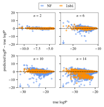
Figure 2: We evaluate the performance of normalizing flows on a mixture model, comprised of five Gaussians combined with unequal weights, as the number of dimensions increases. We generate samples from the mixture model in the full 14 dimensions using the package lsbi (Handley et al., 2023a, b) and drop the required number of columns to get samples in lower dimensions. We then train a normalizing flow using margarine on each set of samples, and compare the true log probability with the log probability predicted by the NF (blue). The black dashed line shows where the points would sit if the two perfectly matched. We also fit a five component Gaussian mixture model to each set of samples using lsbi and plot the log probability predictions of this too (orange). Since this model is in theory capable of fitting the distribution exactly, it could be taken to represent an upper bound on how well the task of density estimation can be performed in practice on this example. In lower dimensions, the NF performs well, albeit with slightly more scatter compared to the lsbi result. By $n=10$, however, the NF exhibits a significant decline in performance compared to the lsbi fit, with the most severe deterioration in the tails of the distribution. By $n=14$, both fits perform poorly. The arrows represent that there are points which lie outside the plot area. The full code to reproduce this plot, including details of how the mixture model was generated, can be found at Prathaban et al. (2024).

In this paper, we attempt to address these issues by replacing classic normalizing flows with what we christen $\beta$-flows.

3.1 $\beta$-flows and the connection with statistical mechanics

There is an analogy to be made between the nested sampling algorithm and statistical mechanics (Habeck, 2015). In particular, the Bayesian evidence may be related to the partition function, if we consider the parameters $\theta$ to describe the microstate of a system with potential energy equal to the negative log-likelihood. The density of states may be expressed as:

$$g(E)=\int\delta[E-E(\theta)]\pi(\theta)d\theta,$$ (15)

where the prior is interpreted as the distribution of all possible states. An isolikelihood contour at $\mathcal{L}^{\ast}$ then corresponds to an energy limit $\epsilon=-\textrm{log}(\mathcal{L}^{\ast})$. We can then see that the fractional prior volume, $X$, is simply the cumulative density of states, as a function of energy, rather than likelihood:

$$X(\epsilon)=\int_{E(\theta)<\epsilon}\pi(\theta)d\theta=\int_{-\infty}^{\epsilon}g(E)dE.$$ (16)

The partition function at inverse canonical temperature $\beta$ may be rewritten as:

$$Z(\beta) =\int e^{-\beta E}g(E)dE=\int e^{-\beta\times-\textrm{log}\mathcal{L}(\theta)}\pi(\theta)d\theta$$

$$=\int\mathcal{L}(\theta)^{\beta}\pi(\theta)d\theta=\int\mathcal{L}(X)^{\beta}dX$$ (17)

This inverse temperature ranges from $\beta=0$, corresponding to an integral over the prior, to $\beta=1$, recovering the Bayesian evidence integral from equation 4. Though nested sampling is not thermal, it can simulate any temperature (Skilling, 2006), meaning the partition function may be evaluated at any $\beta$ after the run (Figure 3).

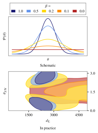
Figure 3: Nested sampling can emulate any temperature. The posterior has an inverse temperature of $\beta=1$ and the prior has an inverse temperature of $\beta=0$. In-between temperature represent intermediate distributions. This is illustrated first on a more straightforward case where the posterior is a Gaussian and the prior is uniform (top panel). As $\beta$ decreases from $1$ to $0$, the distribution widens. The bottom panel shows the two-dimensional $1\sigma$ contours recovered from a simulated binary black hole merger for the luminosity distance, $d_{L}$, and the zenith angle between the total angular momentum and the line of sight, $\theta_{\mathrm{JN}}$. The posterior samples are re-weighted according to equation 18 to generate the distributions at various temperatures. Between $\beta=0.1$ and $\beta=0.2$, the distribution begins to split into two modes; in the statistical mechanics analogy, this is akin to a phase transition at the critical temperature.

Generating samples at any inverse temperature involves modifying the posterior weights of the dead points from equation 6 to

$$p_{i}(\beta)=\frac{w_{i}\mathcal{L}_{i}^{\beta}}{\mathcal{Z}(\beta)}.$$ (18)

$\mathcal{Z}(\beta)$ is evaluated from equation 17. This functionality is provided by the package anesthetic (Handley, 2019). Typically, normalizing flows (NF) are trained only on the posterior samples, drawn from the $\beta=1$ distribution. As such, any information about the posterior and underlying likelihood functions encapsulated in the $\beta<1$ intermediate distributions are discarded. The idea of $\beta$-flows is to incorporate this additional tail information to better learn the posterior.

3.2 Training $\beta$-flows

The goal is to learn a target distribution $\mathcal{P}(\theta)$ conditioned on the inverse temperature $\beta$ for samples from a NS run. We use conditional normalizing flows to transform samples from the multivariate base distribution $z\sim\mathcal{N}(0,1)$ onto $\mathcal{P}(\theta|\beta)$, where $\theta$ are drawn from the low resolution nested sampling run, with weights given by equation 18. For any bijective transformation $f_{\phi}$, we can calculate the probability of a set of samples given $\beta$ by

$$P_{\phi}(\theta|\beta)=\mathcal{N}(f_{\phi}(\theta,\beta)|\mu=0,\sigma=1)\left|\frac{df_{\phi}(\theta,\beta)}{d\theta}\right|.$$ (19)

$\phi$ are the parameters of the neural network. We parameterize $f_{\phi}$ as a conditional masked auto-regressive (MAF) flow and train on a weighted reverse KL divergence (Bevins et al., 2023; Alsing & Handley, 2021):

$$\mathbb{L}=-\frac{1}{\sum p_{i}}\sum p_{i}(\beta)\textrm{log}P_{\phi}(\theta|\beta).$$ (20)

We give the network samples weighted by various sets of $p(\beta)$, where $\beta$ ranges from $0$ to $1$. The training data therefore consists of $\{\theta,p(\beta),\beta\}$, in contrast to normal NFs, where we train with $\{\theta,p(\beta=1)\}$.

As $\beta$ increases from $0$ to $1$, the KL divergence between the weighted dead points and the prior increases non-linearly. The maximum KL divergence occurs at $\beta=1$, but the most rapid change happens at low $\beta$.

$$\mathcal{D}_{\textrm{KL}}=\frac{1}{\sum_{i}p_{i}(\beta)}\sum_{i}p_{i}(\beta)\textrm{log}\frac{P(\theta|\beta)}{\pi(\theta)}.$$ (21)

As such, instead of building the training data from $\beta$ values drawn uniformly from $[0,1]$, we define a $\beta$ schedule such that the change in KL divergence between subsequent sets of weighted dead points is constant. We choose a fixed number of $\beta$ values we want to train on first, and then calculate the exact $\beta$s between $0$ and $1$ that give equally spaced KL divergences.

Once a $\beta$-flow has been trained on the samples from the low resolution first pass of NS, we then use this as a proposal for the high resolution pass. The flow can emulate not only the $\beta=1$ posterior, but also the intermediate distributions at any $0\leq\beta\leq 1$. We treat $\beta$ as a hyperparameter, similar to the approach in Chen et al. (2022) (though $\beta$ has a different meaning here), and sample over it during the high resolution run. Therefore, if the $\beta=1$ distribution is too narrow compared to the ‘true’ posterior, the proposal can widen itself adaptively at runtime. The repartitioned prior and likelihood functions become

$$\pi^{\ast} =P(\theta|\beta)$$ (22)

$$\mathcal{L}^{\ast} =\frac{\mathcal{L}(\theta)\pi(\theta)}{P(\theta|\beta)},$$ (23)

where this time the repartitioned prior and likelihood depend on $\beta$ (though the final evidences and posteriors will not).

4 Results and discussion

In the following section, we present the results of applying the methods described above applied to both a simulated black hole binary (BBH) signal and a real event from the third Gravitational-Wave Transient Catalogue (GWTC-3). For each analysis, we first perform a low resolution pass of NS using bilby (Ashton et al., 2019), with a slightly modified version (see Appendix A) of the built-in PolyChord sampler (Handley et al., 2015b, a). Next, we train both a standard normalizing flow using margarine (Bevins et al., 2022, 2023) and a $\beta$-flow, with code adapted from margarine, on the weighted posterior samples. Each of these trained flows respectively are then used as the repartitioned prior in a second pass of NS, where the likelihood is also repartitioned according to equation 14. In this second pass, we use the same number of live points as in the first pass to facilitate a direct comparison between methods. However, in typical applications, a higher resolution pass would be used at this stage. All runs employ the IMRPhenomXPHM waveform model (Pratten et al., 2021) and, unless otherwise specified, the standard BBH priors implemented in bilby. Plots are generated using anesthetic (Handley, 2019).

4.1 Injections

We first demonstrate the method on a simulated BBH merger injected into Gaussian noise. We assume a two-detector configuration and inject the signal with the IMRPhenomXPHM waveform model. The binary has chirp mass $\mathcal{M}=28$$M_{\odot}$ and mass ratio $q=0.8$. The spins are non-aligned, with an effective spin parameter $\chi_{\textrm{eff}}=0.27$ and it is located at a luminosity distance $d_{L}=2000$ Mpc. The network matched-filter signal-to-noise ratio (SNR) is $\rho_{mf}=14.8$ and we show the posterior distributions obtained for this signal from a standard nested sampling run in Figures 4 and 5.

For the first step of our method, we perform a low resolution NS run with $n_{\textrm{live}}=200$; this is a much lower number of live points than what is typically used in standard 15-parameter gravitational wave analyses, but is still high resolution enough to capture the main features and modes of the posterior. We then use the weighted samples from this to train both a NF and a $\beta$-flow. The relative performances are shown in Figure 6, where the predicted probabilities from the flows are compared to the posterior probabilities given by NS. Both flows exhibit a fairly large scatter about the target probabilities, typical for a 15-dimensional problem, but the $\beta$-flow performs noticeably better than the NF, particularly in the tails of the distribution.

Each flow is then used as the updated prior for a PR NS run, also with $n_{\textrm{live}}=200$, and the evidences and posteriors obtained from this run are compared to those from standard NS analyses with the same number of live points. Figure 7 shows the log evidence distributions obtained from each PR run and from the original low resolution pass of NS. The results are in excellent agreement, with the error bars on $\log\mathcal{Z}$ being tighter for both the PR runs compared to normal NS, despite using the same number of live points, as predicted by equation 9. We also compare the posteriors obtained from each method, which are plotted in Figures 4 and 5 and again show good agreement between the methods.

Table 1 outlines the relative acceleration provided by each flow compared to normal NS. For a fixed uncertainty in $\mathrm{log}\mathcal{Z}$, given that $n_{\textrm{live}}\propto D_{\mathrm{KL}}$, we may rewrite equation 7 as

$$T\propto T_{\mathcal{L}}\times f_{\textrm{sampler}}\times\mathcal{D}_{\textrm{KL}}^{2}.$$ (24)

Then, the precision-normalized acceleration of the PR run may be approximated as

$$\frac{T^{\textrm{normal NS}}}{T^{\textrm{PR NS}}}=\left(\frac{\mathcal{D}_{\mathrm{KL}}^{\textrm{normal NS}}}{\mathcal{D}_{\mathrm{KL}}^{\textrm{PR NS}}}\right)^{2}$$ (25)

Using PR in conjunction with a trained $\beta$-flow led to almost an order of magnitude improvement in the runtime (see Figure 8). In this instance, the NF performs similarly well to the $\beta$-flow, indicating that the NF has learned a wide enough distribution to avoid sampling inefficiencies in the PR run.

It is important to note at this stage that the quoted speedup factors are calculated purely based on the number of iterations that would be required for a precision-normalized PR run. It does not take into account the changes to $T_{\mathcal{L}}$, the time for a single likelihood evaluation, from including the flows in the likelihood. The $\beta$-flow took longer to evaluate than the NF we used. This also means that for analyses using a waveform model like IMRPhenomXPHM, $T_{\mathcal{L}}$ increases by such a factor that we do not recommend using $\beta$-flows in their current form in these cases. This point is addressed further in the conclusions, including a discussion of future work to speed up the evaluation of our $\beta$-flows, but for now, we intend for the methods presented in this paper to be used in analyses where the evaluation of the gravitational wave likelihood is of comparable cost to the evaluation of the $\beta$-flow. We also note that, strictly speaking, the speedup factors should include the time it takes to perform the original low resolution NS run, but in the typical case where the second pass of NS uses a much larger number of live points, this cost will not contribute significantly to the overall runtime.

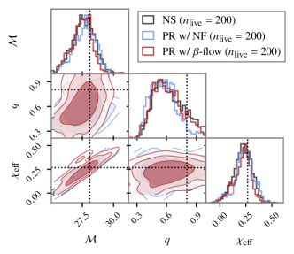
Figure 4: The posteriors obtained on some intrinsic parameters (chirp mass $\mathcal{M}$, mass ratio $q$ and effective spin parameter $\chi_{\mathrm{eff}}$) from standard NS are compared to those obtained using PR with normalizing flows or $\beta$-flows. The results are consistent, showing both the PR methods have managed to recover the same answers as normal NS.

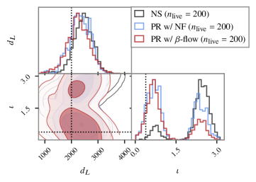
Figure 5: Similarly to 4, the posteriors on the extrinsic parameters, the luminosity distance and inclination, from the two methods are compared. Again, the results are comparable, with the PR NS methods able to achieve this with far fewer likelihood evaluations. The $\beta$-flow method gives less posterior weight in the second mode and more posterior weight in the first mode than the normal NS run, but this could occur from two separate normal NS runs too, due to the stochasticity of NS (Ormondroyd et al., 2024; Handley et al., 2015b). This stochasticity is quantified by the $\text{log}\mathcal{Z}$ error bars that PolyChord outputs for individual clusters.

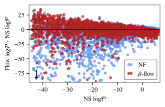
Figure 6: We compare how well both the typical normalizing flow (NF) and the $\beta$-flow (evaluated at $\beta=1$) have learned the rough posterior from the low resolution pass of NS. If the flows have learned the posterior perfectly, the points should lie on the black dashed line. The arrow indicates that there are points which lie below the axes. The $\beta$-flow predictions display much less scatter about this line, showing that the extra tail information from the NS temperature has indeed enabled the flow to learn the posterior better. Although the scatter on the NF seems large, this is an empirically typical performance on a 15-dimensional problem.

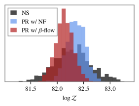
Figure 7: The $\log\mathcal{Z}$ estimates obtained from normal NS, posterior repartitioned NS with a normalizing flow, and posterior-repartitioned NS with a $\beta$-flow are compared. All of the runs are performed with $n_{\textrm{live}}=200$ for easier comparison. The estimates are all consistent with each other, but both the PR runs have smaller error bars, as expected.

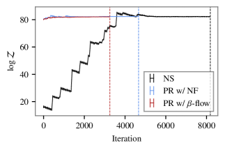
Figure 8: During a normal NS run, the evidence is accumulated as the live points compress towards the peak of the likelihood. The total evidence estimate for normal NS (black) becomes stable late into the run, only after the live points occupy a very small fraction of the prior volume. Because the updated prior for the posterior repartitioned runs is roughly the posterior from the low resolution pass of NS, most of the evidence has already been accumulated very early on in the run. We keep running until the total evidence estimates for the accelerated runs (blue and red) have stabilized. This happens much earlier than for normal NS, and the live points typically still occupy a significant fraction of the prior volume.

type	$n_{\textrm{live}}$	$N_{\textrm{iter}}$	$\sigma_{ln(Z)}$	speedup
normal NS	200	8186	0.352	-
PR NS w/ NF	200	4663	0.177	$\times 7$
PR NS w/ $\beta$-flow	200	3252	0.179	$\times 9$

Table 1: For the simulated event, results of the runs comparing normal NS to posterior-repartitioned NS (PR NS) are shown. $N_{i}ter$ is the total number of iterations, $i$, of the algorithm that were performed, and is proportional to the number of likelihood evaluations. Both the run using a typical normalizing flow and using a $\beta$-flow finish significantly sooner than normal NS. The final column shows the precision-normalized speedup, calculated by using equation 9 to work out how many live points we would need to run with in order to match the $\log\mathcal{Z}$ uncertainty of the normal NS run, and then scaling $N_{\textrm{iter}}$ proportionally.

4.2 Real Data

We demonstrate the above methods on the real event, GW191222_033537 (henceforth GW191222) from GWTC-3. As before, we perform a low resolution pass of NS on which we train both flows. This time, however, we use $350$ live points. The posterior for this event is more complex and has more multi-modality than the simulated example above, so we give the flows more samples to train on in order to give them a better chance of learning these features accurately.

As shown in Figure 9, once again the $\beta$-flow is able to learn the rough posterior from the NS run more accurately, and is better at predicting deep tail probabilities than the NF. However, both flows exhibit a wider spread than before at the highest log probability values, and there is a ‘tail’ of under-predictions for certain samples from the peak of the posterior. This is indicative of the fact that the full multi-modality of the NS posterior has not been captured by either flow, though the NF does perform significantly worse. This is key to understanding the final results.

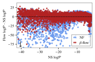
Figure 9: The $\beta$-flow once again performs better at predicting the log probability given by NS. This time, both flows have a larger spread at higher log probabilities and a ‘tail’ of points below the black dashed line. Again, the arrow indicates that there are points which lie below the axes. The NF heavily under-predicts the posterior probability of certain samples, which is indicative of the fact that it has failed to capture the multi-modality of the rough posterior.

To properly verify whether we have recovered the correct posteriors for this real event, we compare our posteriors from the accelerated methods to those from a higher resolution ($n_{\mathrm{live}}=2000$) standard NS run. Since the NF does not learn the multi-modality of the posterior well enough, it sets the proposal for the PR run such that certain modes are only included in the prior with very low probabilities. This leads to a biasing of the final posteriors, shown in Figures 10 and 11. The $\beta$-flow also doesn’t fully learn the multi-modality of the posterior, but since it acts as an adaptive prior at runtime, able to draw samples from the distribution at any inverse temperature, it does not completely cut off important regions of the parameter space in the same way the NF does. Looking at the posteriors in Figure 11, we can indeed see that the $\beta=1$ distribution was too narrow and excluded regions of the parameter space with non-negligible posterior weight. Otherwise, we would expect to see a roughly uniform posterior on $\beta$, but instead we see that $\beta=1$ has a low posterior probability.

The evidence calculated by PR NS using the NF also reflects this bias (Figure 12). The results are incompatible with those from normal NS, and is another sign that regions of the parameter space with significant posterior weight were missed due to the updated prior being too narrow. Once again, because the $\beta$-flow can emulate any temperature, it is robust to these issues and is able to give equally reliable results as for the simulated example, despite a poorer performance at the posterior density estimation.

Since the $\beta$-flow did not learn the posterior at $\beta=1$ as well as for the simulated case, the speedup given by using this flow as the updated prior was not as large (Figure 13). The exact acceleration provided by PR NS is very sensitive to the accuracy of the density estimation. However, the precision-normalized runtime was still twice as fast as for normal NS and, importantly, we demonstrate the robustness of this method in giving reliable evidences and posteriors, even when the density estimation is relatively poor quality. The worst case scenario of using PR NS with $\beta$-flows is that we get correct evidences and posteriors which take the same amount of time as normal NS (since for a very poor $\beta$-flow we would sample preferentially from the $\beta=0$ distribution, which is the original NS prior). The same cannot be said for PR NS with NFs, however, and the results in this section give an example where this method breaks down completely. For this reason, we recommend using $\beta$-flows in place of NFs when implementing posterior repartitioning.

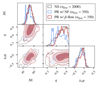
Figure 10: Unlike for the previous simulated signal, using the trained NF as the proposal for PR NS has led to biased results. The NF learned the posterior from the low resolution run poorly, and without the ability to widen itself at runtime, this has produced incorrect posteriors and evidence. The $\beta$-flow is robust to this issue as the proposal is over all values of $\beta$. This means that even if the learned flow is too narrow or has not learned the multi-modality sufficiently well, it can still adapt the proposal at runtime and, in the worst case scenario, samples will simply be drawn from the original prior ($\beta$=0). The posterior on $\beta$ can tell us how poor a proposal the $\beta=1$ learned distribution was.

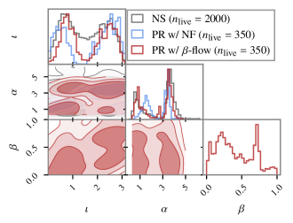
Figure 11: The multi-modality in the extrinsic parameters has caused a biasing effect for PR NS with the NF, since the NF did not learn all modes properly. The posterior on $\beta$, the inverse temperature, for the $\beta$-flow run is also included. If the flow learned the rough posterior well, we would expect to see a uniform posterior on $\beta$. The low posterior probability at $\beta=1$ indicates that the $\beta$-flow had to widen itself at runtime due to the $\beta=1$ distribution being unsuitable as a prior.

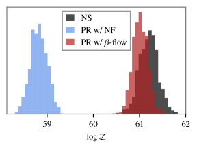
Figure 12: The NF learned the rough posterior from the low resolution run poorly, insufficiently capturing its multi-modality. This has led to a biasing of the final evidences and posteriors, since the proposal from the NF cannot widen itself like the $\beta$-flow can. The $\beta$-flow not only learned the distribution from the first pass of NS better, but also enabled an adaptive proposal at runtime, ensuring robustness against such biases.

type	$n_{\textrm{live}}$	$N_{\textrm{iter}}$	$\sigma_{ln(Z)}$	speedup
normal NS	350	10445	0.211	-
PR NS w/ $\beta$-flow	350	7995	0.171	$\times 2$

Table 2: Normal NS is compared to the PR NS method for real event GW191222. PR NS with the $\beta$-flow is twice as fast as normal NS for a precision-normalized run. This is a smaller speedup than for the simulated example, and this is driven by the fact that the $\beta$-flow was not able to learn the rough posterior from pass 1 as accurately. PR NS with the NF is not shown here; although it was also quicker than normal NS, it gave incorrect posteriors and evidences due to the biased proposal.

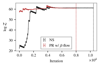
Figure 13: PR NS with the $\beta$-flow terminates before normal NS with the same number of live points. The precision-normalized speedup is less than for the simulated example, but is still a factor of two faster. We don’t show the equivalent line for the NF because it failed to correctly recover the evidence and posterior.

5 Conclusions

In this paper, we outline how posterior repartitioning using normalizing flows can accelerate nested sampling. While we demonstrate these methods with PolyChord, this is a general acceleration technique applicable to a variety of nested sampling algorithms, and does not inherently rely on machine learning to be effective. Bringing together previous work (Chen et al., 2018, 2022; Petrosyan & Handley, 2022; Bevins et al., 2022, 2023; Alsing & Handley, 2021), we demonstrate this method on realistic gravitational wave examples. However, there are a few drawbacks of using traditional normalizing flow architectures in posterior repartitioned nested sampling. Firstly, the amount of acceleration provided by PR NS is highly dependent on the success of the flow in learning the posterior distribution provided by the low resolution nested sampling run. In particular, the more successful the flow is at learning the deep tail probabilities, the sooner we can terminate the high resolution PR run. However, we empirically show that the accuracy of commonly used NF architectures is often poor in the tails of the target distribution, especially as the dimensionality increases. Furthermore, if the distribution learned by the flow is too narrow compared to the true posterior, this can lead to sampling inefficiencies, making the problem harder, and in the worst case scenario can give biased results. We show a real GW case where this occurs.

In order to mitigate these issues, we introduce $\beta$-flows, which are conditional normalizing flows trained on nested samples and conditioned on inverse temperature, $\beta$. $\beta$-flows are shown to be better at predicting deep tail probabilities than traditional normalizing flows, as they have access to intermediate distributions between prior and posterior during training, as opposed to just the posterior samples. Additionally, $\beta$-flows can emulate not just the target posterior distribution itself, which corresponds to $\beta=1$, but also any of these intermediate distributions. At runtime, we sample over different values of $\beta$, meaning that if the $\beta=1$ distribution learned by the flow is indeed too narrow, the repartitioned prior can adaptively widen itself at runtime to mitigate sampling inefficiencies and biases. For the same case on which normal normalizing flows fail, we show that replacing normalizing flows with $\beta$-flows fixes the problem and is thus robust against potential pitfalls.

One current disadvantage of $\beta$-flows is that, due to the flow having to store and call more biases and weights, they take significantly longer to evaluate than more typical normalizing flows. For evaluating the probability of a single sample, they take about $100$ms, $100$ times slower than the NF trained using margarine. This limitation could be ameliorated in a few ways. Firstly, the $\beta$-flow could be implemented in jax, which could significantly reduce this cost. Moreover, NFs and $\beta$-flows are designed to evaluate batches of samples at once, and so this cost does scale linearly with the number of samples. For a set of $10,000$ samples, the $\beta$-flows only take twice as long to evaluate them as for a single sample, and only take $4$ times as long as a flow using margarine. Therefore, if we could implement PR within a nested sampling algorithm which can properly make use of this property of normalizing flows, the cost to evaluate the $\beta$-flow would become negligible. Both of these are promising avenues for future work on this topic, and would make the methods presented in this paper suitable for a wider range of likelihoods. In their current form, they can still be worthwhile implementing in cases where the likelihood itself is of comparable computational cost to the flows.

Currently, the method requires nested samples from the exact likelihood we want to use in our final analysis in order to train the flows. Future work could involve adapting the methodology to enable the $\beta$-flow to learn an approximate distribution, perhaps from a cheaper waveform model, and then use this as a proposal for the high resolution run. This has synergies with likelihood reweighting (Payne et al., 2019) and tempered importance sampling (Saleh et al., 2024). $\beta$-flows also have a connection with continuous normalizing flows (CNFs) and diffusion models, where there is a natural user tunable parameter akin to $\beta$ (Tong et al., 2024). Future work could explore this link, and could explore using CNFs in conjunction with posterior repartitioning too.

Data Availability

All the data used in this analysis, including the relevant nested sampling dataframes, can be obtained from Prathaban et al. (2024). We include a notebook with all the code to reproduce the plots in this paper. We also include an example python file to show how to implement posterior repartitioning in bilby, with instructions on how to modify the bilby source code. The code we used for training the $\beta$-flows in this paper is publicly available and can be found at Bevins et al. (2024). The modified version of PolyChord used to perform these analyses will also be publicly released.

Appendix A Termination conditions for NS

Posterior repartitioned NS has slightly different properties to normal NS. This means that the usual termination condition that is used for the latter is too cautious for the former. Nested sampling compresses live points exponentially towards the peak of the likelihood function. As they close in on the peak, the likelihood values begin to saturate ($\mathcal{L}_{i}\rightarrow\mathcal{L}_{\textrm{peak}}$) and the fractional volumes become very small ($X_{i}\rightarrow 0$) (Keeton, 2011). As such, beyond a certain point there are diminishing returns for performing further iterations of the algorithm.

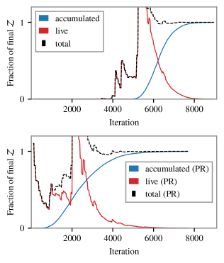
Figure 14: As described in Keeton (2011), the total evidence estimate varies throughout a typical NS run. In typical NS (top panel), the accumulated evidence before we reach the bulk of the posterior is very low, due to small likelihood values. When the live points enter the posterior bulk, this accumulated evidence steadily increases, until the likelihoods saturate and the fractional prior volume changes become negligible. The estimate of the evidence remaining in the live points is much more unstable, and is initially dominated by a single live point with the highest weight, $w_{i}\mathcal{L}_{i}$. It spikes and falls rapidly as a new live point is found which temporarily dominates the live evidence, and hence the total evidence estimate also changes. This total evidence estimate usually only becomes stable once the fractional evidence remaining in the live points is small, making this a robust proxy for the stopping criterion in normal NS. When doing posterior repartitioning, however, the total evidence estimate may stabilize before the live evidence fraction has fallen by the required amount (bottom panel). In these cases, the algorithm may continue for many more iterations without any additional benefit. Here, the usual termination condition is too cautious and should be framed directly in terms of the total evidence estimate instead.

At each iteration $k$, the estimated total evidence is the sum of the accumulated evidence and the estimated evidence remaining in the live points.

$$\mathcal{Z}_{\mathrm{tot}}=\mathcal{Z}_{\mathrm{dead}}+\mathcal{Z}_{\mathrm{live}}\approx\sum_{i=1}^{k}\mathcal{L}_{i}(X_{i-1}-X_{i})+\bar{\mathcal{L}}_{\textrm{live}}X_{k}.$$ (26)

$\bar{\mathcal{L}}_{\textrm{live}}$ represents the average likelihood of the live points at iteration $k$, and $X_{k}$ is the remaining fractional volume.

Figure 14 shows the evolution of each of these terms as a function of the iteration number. Initially, since the deleted points have not yet reached the bulk of the posterior, the total accumulated evidence is very small due to low likelihoods. Once the bulk of the posterior is reached, the accumulated evidence builds up rapidly as the likelihood increases, until the likelihood flattens out near the peak and the fractional volume changes become negligible. At this point, the accumulated evidence saturates.

The estimated live evidence is very unstable to begin with. It is usually dominated by a single live point which lies in the posterior, and rises sharply when a new live point is found which temporarily becomes the main contributor, falling again as the fractional prior volume decreases. Once the live points are completely contained within the bulk of the posterior, the estimated live evidence begins to fall smoothly, unless previously missed modes are found. The total evidence is also unstable at the beginning, dominated by the live evidence, but starts to become stable once we enter the posterior bulk. Ideally, we would terminate our run once this estimated total evidence has become completely stable and does not change significantly as we perform further iterations of the algorithm.

In most cases, a proxy for this is to stop when the estimated live evidence is some very small fraction of the total accumulated evidence, and this is the default termination condition in many popular NS implementations (Ashton et al., 2022). In the specific case of posterior repartitioning, however, this is perhaps too cautious a stopping criterion. In the extreme case where our trained flow has perfectly learned the posterior distribution, we could terminate our high resolution PR run almost immediately, since although performing further iterations of the algorithm would increase the accumulated evidence and decrease the live evidence, it would make no difference to the total evidence estimate. Even in the case where the flow has imperfectly learned the posterior, much of the discrepancy is likely to be in the tails of the distribution. As such, the total evidence estimate would still likely stabilize well before the live evidence fraction falls below the usual threshold (see e.g. Figure 8). As a result, in the above analyses we modified PolyChord to set the termination condition for the run in terms of the estimated total evidence directly, instead of the live evidence fraction. For normal NS, this resulted a very similar end point to the default condition for all the examples we ran.

References

- Albert (2020) Albert J. G., 2020, JAXNS: a high-performance nested sampling package based on JAX (arXiv:2012.15286), https://arxiv.org/abs/2012.15286
- Alsing & Handley (2021) Alsing J., Handley W., 2021, MNRAS, 505, L95
- Anstey et al. (2021) Anstey D., de Lera Acedo E., Handley W., 2021, Monthly Notices of the Royal Astronomical Society, 506, 2041
- Ashton et al. (2019) Ashton G., et al., 2019, Astrophys. J. Suppl., 241, 27
- Ashton et al. (2022) Ashton G., et al., 2022, Nature Reviews Methods Primers, 2, 39
- Baldock et al. (2017) Baldock R. J. N., Bernstein N., Salerno K. M., Pártay L. B., Csányi G., 2017, Physical Review E, 96
- (7) Barbary K., , nestle: Pure Python, MIT-licensed implementation of nested sampling algorithms for evaluating Bayesian evidence., https://github.com/kbarbary/nestle.git
- Bevins et al. (2022) Bevins H., Handley W., Lemos P., Sims P., de Lera Acedo E., Fialkov A., 2022, arXiv e-prints, p. arXiv:2207.11457
- Bevins et al. (2023) Bevins H. T. J., Handley W. J., Lemos P., Sims P. H., de Lera Acedo E., Fialkov A., Alsing J., 2023, MNRAS, 526, 4613
- Bevins et al. (2024) Bevins H., et al., 2024, beta-flows, https://github.com/htjb/beta-flows.git
- Brewer et al. (2010) Brewer B. J., Pártay L. B., Csányi G., 2010, Diffusive Nested Sampling (arXiv:0912.2380), https://arxiv.org/abs/0912.2380
- Buchner (2021) Buchner J., 2021, UltraNest – a robust, general purpose Bayesian inference engine (arXiv:2101.09604), https://arxiv.org/abs/2101.09604
- Chen et al. (2018) Chen X., Hobson M., Das S., Gelderblom P., 2018, Improving the efficiency and robustness of nested sampling using posterior repartitioning (arXiv:1803.06387), https://arxiv.org/abs/1803.06387
- Chen et al. (2022) Chen X., Feroz F., Hobson M., 2022, Bayesian posterior repartitioning for nested sampling (arXiv:1908.04655), https://arxiv.org/abs/1908.04655
- Corsaro & Ridder (2015) Corsaro E., Ridder J. D., 2015, EPJ Web of Conferences, 101, 06019
- Dax et al. (2021) Dax M., Green S. R., Gair J., Macke J. H., Buonanno A., Schölkopf B., 2021, Phys. Rev. Lett., 127, 241103
- Duane et al. (1987) Duane S., Kennedy A. D., Pendleton B. J., Roweth D., 1987, Physics letters B, 195, 216
- Fan et al. (2012) Fan Y., Nott D. J., Sisson S. A., 2012, arXiv e-prints, p. arXiv:1212.1479
- Feroz & Hobson (2008) Feroz F., Hobson M. P., 2008, Monthly Notices of the Royal Astronomical Society, 384, 449–463
- Feroz et al. (2009) Feroz F., Hobson M. P., Bridges M., 2009, Monthly Notices of the Royal Astronomical Society, 398, 1601–1614
- Field et al. (2023) Field S. E., et al., 2023, Physical Review D, 108, 123025
- Gessey-Jones et al. (2024) Gessey-Jones T., Pochinda S., Bevins H. T. J., Fialkov A., Handley W. J., de Lera Acedo E., Singh S., Barkana R., 2024, MNRAS, 529, 519
- Habeck (2015) Habeck M., 2015. pp 121–129, doi:10.1063/1.4905971
- Handley (2019) Handley W., 2019, Journal of Open Source Software, 4, 1414
- Handley et al. (2015a) Handley W. J., Hobson M. P., Lasenby A. N., 2015a, Monthly Notices of the Royal Astronomical Society: Letters, 450, L61–L65
- Handley et al. (2015b) Handley W. J., Hobson M. P., Lasenby A. N., 2015b, Monthly Notices of the Royal Astronomical Society, 453, 4385–4399
- Handley et al. (2023b) Handley W., et al., 2023b, lsbi, https://github.com/handley-lab/lsbi.git
- Handley et al. (2023a) Handley W., et al., 2023a, In preparation
- Hastings (1970) Hastings W. K., 1970, Biometrika, 57, 97
- Higson (2018) Higson E., 2018, Journal of Open Source Software, 3, 965
- Higson et al. (2018) Higson E., Handley W., Hobson M., Lasenby A., 2018, Statistics and Computing, 29, 891–913
- Keeton (2011) Keeton C. R., 2011, Monthly Notices of the Royal Astronomical Society, 414, 1418–1426
- Kester & Mueller (2021) Kester D., Mueller M., 2021, BayesicFitting, a PYTHON Toolbox for Bayesian Fitting and Evidence Calculation (arXiv:2109.11976), https://arxiv.org/abs/2109.11976
- Khan et al. (2016) Khan S., Husa S., Hannam M., Ohme F., Pürrer M., Forteza X. J., Bohé A., 2016, Physical Review D, 93
- Kobyzev et al. (2021) Kobyzev I., Prince S. J., Brubaker M. A., 2021, IEEE Transactions on Pattern Analysis and Machine Intelligence, 43, 3964–3979
- Krishna et al. (2023) Krishna K., Vijaykumar A., Ganguly A., Talbot C., Biscoveanu S., George R. N., Williams N., Zimmerman A., 2023, Accelerated parameter estimation in Bilby with relative binning (arXiv:2312.06009), https://arxiv.org/abs/2312.06009
- Matthews et al. (2022) Matthews A. G. D. G., Arbel M., Rezende D. J., Doucet A., 2022, arXiv e-prints, p. arXiv:2201.13117
- Metropolis et al. (1953) Metropolis N., Rosenbluth A. W., Rosenbluth M. N., Teller A. H., Teller E., 1953, Journal of Chemical Physics, 21, 1087
- Morrás et al. (2023) Morrás G., Nuño Siles J. F., García-Bellido J., 2023, Physical Review D, 108
- Moss (2020) Moss A., 2020, Monthly Notices of the Royal Astronomical Society, 496, 328–338
- Mukherjee et al. (2006) Mukherjee P., Parkinson D., Liddle A. R., 2006, The Astrophysical Journal, 638, L51–L54
- Neal (2011) Neal R. M., 2011, Handbook of Markov Chain Monte Carlo, 2, 2
- Ormondroyd et al. (2024) Ormondroyd A., et al., 2024, In preparation
- Paige & Wood (2016) Paige B., Wood F., 2016, arXiv e-prints, p. arXiv:1602.06701
- Papamakarios & Murray (2015) Papamakarios G., Murray I., 2015, Distilling intractable generative models
- Papamakarios & Murray (2016) Papamakarios G., Murray I., 2016, arXiv e-prints, p. arXiv:1605.06376
- Parkinson et al. (2006) Parkinson D., Mukherjee P., Liddle A. R., 2006, Physical Review D, 73
- Payne et al. (2019) Payne E., Talbot C., Thrane E., 2019, Physical Review D, 100
- Petrosyan & Handley (2022) Petrosyan A., Handley W., 2022, SuperNest: accelerated nested sampling applied to astrophysics and cosmology, doi:10.48550/arXiv.2212.01760
- Pochinda et al. (2023) Pochinda S., et al., 2023, arXiv e-prints, p. arXiv:2312.08095
- Prathaban et al. (2024) Prathaban M., Bevins H., Handley W., 2024, Accelerated nested sampling with -flows for gravitational waves, doi:10.5281/zenodo.14198699, https://doi.org/10.5281/zenodo.14198699
- Pratten et al. (2021) Pratten G., et al., 2021, Physical Review D, 103
- Saleh et al. (2024) Saleh B., Zimmerman A., Chen P., Ghattas O., 2024, Tempered Multifidelity Importance Sampling for Gravitational Wave Parameter Estimation (arXiv:2405.19407), https://arxiv.org/abs/2405.19407
- Skilling (2006) Skilling J., 2006, Bayesian Analysis, 1, 833
- Smith et al. (2016) Smith R., Field S. E., Blackburn K., Haster C.-J., Pürrer M., Raymond V., Schmidt P., 2016, Physical Review D, 94
- Speagle (2020) Speagle J. S., 2020, Monthly Notices of the Royal Astronomical Society, 493, 3132–3158
- Thrane & Talbot (2019) Thrane E., Talbot C., 2019, Publications of the Astronomical Society of Australia, 36
- Tong et al. (2024) Tong A., Fatras K., Malkin N., Huguet G., Zhang Y., Rector-Brooks J., Wolf G., Bengio Y., 2024, Improving and generalizing flow-based generative models with minibatch optimal transport (arXiv:2302.00482), https://arxiv.org/abs/2302.00482
- Trassinelli (2017) Trassinelli M., 2017, doi:10.1016/j.nimb.2017.05.030, 408, 301–312
- Trassinelli (2019) Trassinelli M., 2019, Proceedings, 33
- Trassinelli & Ciccodicola (2020) Trassinelli M., Ciccodicola P., 2020, Entropy, 22
- Veitch et al. (2015a) Veitch J., et al., 2015a, Physical Review D, 91
- Veitch et al. (2015b) Veitch J., et al., 2015b, Physical Review D, 91
- Veitch et al. (2024) Veitch J., et al., 2024, johnveitch/cpnest: v0.11.7, doi:10.5281/zenodo.12801702, https://doi.org/10.5281/zenodo.12801702
- Vinciguerra et al. (2017) Vinciguerra S., Veitch J., Mandel I., 2017, Classical and Quantum Gravity, 34, 115006
- Williams et al. (2021) Williams M. J., Veitch J., Messenger C., 2021, Phys. Rev. D, 103, 103006