Oscillatory instability and stability of stationary solutions in the parametrically driven, damped nonlinear Schrödinger equation

Abstract

We found two stationary solutions of the parametrically driven, damped nonlinear Schrödinger equation with nonlinear term proportional to $|\psi(x,t)|^{2\kappa}\psi(x,t)$ for positive values of $\kappa$. By linearizing the equation around these exact solutions, we derive the corresponding Sturm-Liouville problem. Our analysis reveals that one of the stationary solutions is unstable, while the stability of the other solution depends on the amplitude of the parametric force, damping coefficient, and nonlinearity parameter $\kappa$. An exceptional change of variables facilitates the computation of the stability diagram through numerical solutions of the eigenvalue problem as a specific parameter $\varepsilon$ varies within a bounded interval. For $\kappa<2$ , an oscillatory instability is predicted analytically and confirmed numerically. Our principal result establishes that for $\kappa\geq 2$, there exists a critical value of $\varepsilon$ beyond which the unstable soliton becomes stable, exhibiting oscillatory stability.

1 Introduction

The nonlinear Schrödinger (NLS) soliton under parametric excitation captures the dynamics of small-amplitude breathers of the easy-plane ferromagnet and the long Josephson junction under the influence of the parametric pumping and dissipation [1, 2]. Additionally, it accounts for various phenomena, including the repulsive behavior of the double-solitons observed in an oscillating water channel of finite length [3], the excited surface-waves solitons reported in Ref. [4, 5], and the non-propagating hydrodynamic soliton under confinement [6].

Constant and spatio-temporal parametric forces lead to moving NLS solitary waves which break the integrability of the NLS equation. In the former case, stable non-propagating and moving solitons coexist at low driving strengths, while strongly forced solitons are stable only at high speeds [7]. For time and space dependency of the force, the soliton can oscillate around a certain position; and two empirical stability criteria based on the collective coordinate approach have been applied to determine the regions of stability [8].

Time-dependent parametric pumping in the NLS equation facilitates the creation and annihilation of solitons [9], the existence of soliton bound states [10], models small-amplitude breathers of the parametrically driven, damped Landau-Lifshitz and sine-Gordon equations [2], and stabilizes the damped solitons [11, 1, 7]. Unlike the nonlinear Klein-Gordon equations [12, 13, 14], in which topological solitary waves exhibit robustness in the presence of damping, the nonlinear Schrödinger soliton is damped and eventually fades away under similar conditions. However, an additional parametric force $r\,e^{2it}\Psi^{\star}(x,t)$ with amplitude $r$ can compensate the dissipative effects $i\,\rho\,\Psi(x,t)$ with dissipation coefficient $\rho$ and stabilize the stationary solutions of the parametrically driven, damped nonlinear Schrödinger equation

$$i\Psi_{t}+\Psi_{xx}+2|\Psi|^{2\,\kappa}\Psi=re^{2it}\Psi^{\star}-i\rho\Psi.$$ (1)

Specifying $\kappa=1$, this perturbation even permits the existence of two exact stationary solutions [15]. Barashenkov, Bogdan and Korobov shown that one of these two solutions is unstable [1], while the other solution remains stable in a certain region of the plane $\rho$-$r$. The solution initially stable may become unstable due to a collision of two internal modes (mechanism of oscillatory instability [16]).

The aim of the current study is twofold: First, to extend the search for stationary solutions of Eq. (1) with arbitrary nonlinearity parameter $\kappa>0$. Second to conduct a stability analysis that explores the dependence on $\kappa$. The case $\kappa\geq 2$, where the NLS soliton is unstable in the absence of parametric forcing and dissipation, is of particular interest. This soliton was stabilized by incorporating an external potential with supersymmetry and parity-time symmetry [17]. Here, we show that it can be stabilized through the combined effect of damping and parametric force. The unstable soliton may become stable due to the resonance between two internal modes moving in the real axis (mechanism of oscillatory stability).

We found that Eq. (1) possesses two exact stationary solutions, denoted by $\Psi_{\pm}(x,t)$. Notably, the conditions for existence of $\Psi_{\pm}(x,t)$ are independent of $\kappa$. While both solutions share the same functional form, $\Psi_{-}(x,t)$ has a lower amplitude than $\Psi_{+}(x,t)$. We demonstrate that the former solution is always unstable owing to the presence of a positive real eigenvalue in the spectrum of the corresponding Sturm-Liouville problem, which is obtained from the linearization of Eq. (1) around $\Psi_{-}(x,t)$. Subsequently, we provide a parametrization that reduces the parameter space, enabling us to obtain the stability curve, $r(\rho)$, that separates the stable and unstable regions for each value of $\kappa$, including $\kappa\geq 2$.

The paper is organized as follows. In Sec. 2, from the continuity equations we derive the conditions for the existence of two stationary solutions of Eq. (1), and explicitly find them. Section 3 focuses on linear stability analysis by linearizing the considered NLS equation around its stationary solution and by obtaining the corresponding Sturm-Liouville problem. In Sec. 4, we numerically solve the eigenvalue problem and compute the stability curve $r(\rho)$, which delineates the boundary between the stable and unstable regions. In appendix A we prove that $\Psi_{-}(x,t)$ is unstable, while in appendix B we analytically demonstrate that $\Psi_{+}(x,t)$ exhibits oscillatory instability for $\kappa<2$ whenever  a complex quadruplet emerges. Finally, we summarize the main results and conclusions in Sec. 5.

2 Parametrically driven and damped NLS soliton for $\kappa>0$

The Eq. (1) can be derived by inserting the Lagrangian density

$$\mathcal{L}=i\frac{\Psi_{t}\Psi^{\star}-\Psi_{t}^{\star}\Psi}{2}-|\Psi_{x}|^{2}+\frac{2}{\kappa+1}|\Psi|^{2(\kappa+1)}-r\frac{e^{2ti}(\Psi^{\star})^{2}+e^{-2ti}\Psi^{2}}{2},$$ (2)

and the dissipation function

$$\mathcal{F}=-i\rho(\Psi_{t}\Psi^{\star}-\Psi_{t}^{\star}\Psi),$$ (3)

into the Euler-Lagrange equation, which has been generalized to include a dissipation term on the right-hand side [8].

Equation (1) for $\kappa=1$ has been derived from the Landau-Lifshitz equation, which describes the magnetization dynamics of ferromagnetic materials [1]. In this model the azimuthal angle of the unit vector of magnetization $\vec{m}$ is governed by the driven sine-Gordon equation, while a linear combination of the $y$ and $z$ components of $\vec{m}$ is directly related to the solution $\Psi(x,t)$ of Eq. (1).

The nonlinear parameter $\kappa$ and the parametric force explicitly modifies the energy density as follows

$$E =\int_{-\infty}^{+\infty}\left(|\Psi_{x}|^{2}-\frac{2}{\kappa+1}|\Psi|^{2(\kappa+1)}+r\frac{e^{2ti}(\Psi^{\star})^{2}+e^{-2ti}\Psi^{2}}{2}\right)\,dx.$$ (4)

From (4), it can be deduced that if the frequency of stationary solution is locked with the half of frequency of the parametric force such that $\Psi(x,t)\propto e^{i\,t}$, then its energy is constant. Indeed, by inserting the ansatz

$$\Psi(x,t) =\psi(x)e^{-\frac{i}{2}\,\theta(x)}e^{it}$$ (5)

into Eq. (4), it can be verified that the energy, as well as the momentum

$$P=\frac{i}{2}\int_{-\infty}^{+\infty}(\Psi\,\Psi_{x}^{\star}-\Psi^{\star}\,\Psi_{x})\,dx,$$ (6)

and the norm

$$N=\int_{-\infty}^{+\infty}|\Psi|^{2}\,dx$$ (7)

are time independent. This observation is counterintuitive since the time derivative of these quantities

$$\frac{dE}{dt} =\int_{-\infty}^{+\infty}\left\{\mathcal{F}+i\,r[e^{2ti}(\Psi^{\star})^{2}-e^{-2ti}\Psi^{2}]\right\}\,dx,$$ (8)

$$\frac{dP}{dt} =\int_{-\infty}^{+\infty}\left\{\rho\,i(\Psi^{\star}\,\Psi_{x}-\Psi\,\Psi_{x}^{\star})+r\,(e^{2ti}\Psi^{\star}\,\Psi_{x}^{\star}+e^{-2ti}\Psi\,\Psi_{x})\right\}\,dx,$$ (9)

$$\frac{dN}{dt} =\int_{-\infty}^{+\infty}\left\{-2\rho|\Psi|^{2}+i\,r[e^{-2ti}\Psi^{2}-e^{2ti}(\Psi^{\star})^{2}]\right\}\,dx,$$ (10)

are in general not zero due to the non-vanishing source terms in the continuity equations of the energy, the momentum, and the norm, respectively. However, by inserting the ansatz (5) for stationary solution into the r.h.s of Eqs. (8)–(10), it can be shown that all these integrals vanish whenever $\theta(x)=\Theta$ satisfies

$$\sin(\Theta) =\frac{\rho}{r}.$$ (11)

Therefore, either

$$\Theta=\Theta_{+} =\arcsin\left(\frac{\rho}{r}\right),$$ (12)

or

$$\Theta=\Theta_{-} =\pi-\arcsin\left(\frac{\rho}{r}\right).$$ (13)

In both cases, $\psi(x)$ satisfies the equation

$$\psi_{xx}-[1+r\cos(\Theta)]\psi+2\psi^{2\,\kappa+1}=0,$$ (14)

and its solution is given by

$$\psi_{\pm}(x)=B_{\pm}\sech^{1/\kappa}[\kappa\,\sqrt{\omega_{\pm}}\,x],\quad B_{\pm}=\left(\frac{\omega_{\pm}(\kappa+1)}{2}\right)^{1/2\,\kappa},$$ (15)

$\omega_{\pm}\equiv 1+r\cos(\Theta)=1\pm\sqrt{r^{2}-\rho^{2}}>0$, $r\geq\rho$. Since $\omega_{-}>0$, $\rho<r<\sqrt{1+\rho^{2}}$ for $\Psi_{-}(x,t)$. Therefore, the two stationary solutions of the parametrically driven, damped NLS Eq. (1) are

$$\Psi_{\pm}(x,t)=B_{\pm}\sech^{1/\kappa}[\kappa\sqrt{\omega_{\pm}}x]e^{i\,t-i\Theta_{\pm}/2}.$$ (16)

For the specific value of $\kappa=1$, this solution agrees with Eqs. (4)-(6) of Ref. [18]. Interestingly, the parameter $\kappa$ influences both the amplitude, and the width of the soliton. Specifically, as $\kappa$ decreases, the soliton becomes wider and taller. However, the two conditions for the existence of these solutions, namely that its frequency is locked to half the frequency of the parametric drive, and that its phase satisfies Eqs. (12)–(13), are independent of $\kappa$.

A direct stability analysis of this solution requires the variation of $\kappa$, $r$ and $\rho$. In the next section, we will provide a linear stability analysis using an exceptional change of variables [1], which simplifies the derivation of the curve $r(\rho)$ that separates stable and unstable regions for each value of $\kappa$.

3 Linear stability analysis

We linearize Eq. (1) around its stationary solution (16), by substituting $\Psi(x,t)=[\psi_{\pm}(x)+u(x,t)]e^{i\,t-i\Theta_{\pm}/2}$ into Eq.  (1). Here, $\psi_{\pm}(x)$ is given by Eq. (15), and the small perturbation $u(x,t)$ can be a complex function, satisfying

$$iu_{t}-u+u_{xx}+2\,(\kappa+1)\psi_{\pm}^{2\,\kappa}u+2\,\kappa\psi_{\pm}^{2\,\kappa}u^{\star}=re^{i\Theta_{\pm}}u^{\star}-i\rho u.$$ (17)

Therefore, the real and the complex parts of $u(x,t)=e^{-\rho\,t}\,[f(x,t)+i\,g(x,t)]$ satisfy

$$f_{t}-\rho f =\left(-\frac{d^{2}}{dx^{2}}-2\psi_{\pm}^{2\,\kappa}+1-r\,\cos(\Theta_{\pm})\right)\,g.$$ (18)

$$-g_{t}-\rho\,g =\left(-\frac{d^{2}}{dx^{2}}-2(2\,\kappa+1)\psi_{\pm}^{2\,\kappa}+1+r\,\cos(\Theta_{\pm})\right)\,f.$$ (19)

With this definition of $u(x,t)$ both equations are influenced by the damping in the same way. These equations can be rewritten as follows:

$$f_{T}-\widetilde{\rho}f =L_{0}\,g,$$ (20)

$$-g_{T}-\widetilde{\rho}\,g =L_{1}\,f,$$ (21)

where the operators $L_{0},L_{1}$ are defined as

$$L_{0} =-\frac{d^{2}}{dX^{2}}+1-\varepsilon_{\pm}-(2-\varepsilon_{\pm})\psi_{\pm}^{2\,\kappa},$$ (22)

$$L_{1} =-\frac{d^{2}}{dX^{2}}+1-(2-\varepsilon_{\pm})(2\,\kappa+1)\psi_{\pm}^{2\,\kappa},$$ (23)

and $X=\sqrt{\omega_{\pm}}x$, $T=\omega_{\pm}t$, $\varepsilon_{\pm}=2(1-1/\omega_{\pm})$, and $\widetilde{\rho}=\rho/\omega_{\pm}$. The term $(2-\varepsilon_{\pm})\psi_{\pm}^{2\,\kappa}=(\kappa+1)\,\sech^{2}(\kappa X)$. For $\kappa=1$ these operators agree with the studied ones in Ref. [1].

Notice that the function $\psi_{\pm}(X)$ satisfies

$$\psi_{XX}-\psi+(2-\varepsilon_{\pm})\psi^{2\,\kappa+1}=0,$$ (24)

with the parameters $\varepsilon_{-}\in(-\infty,0)$ and $\varepsilon_{+}\in[0,2)$, respectively. When $\varepsilon_{+}=0$, $r=\rho$, and the solution of this equation reduces to the soliton of the nonlinear Schrödinger equation with specific phase.

Lets consider first, the stability of $\Psi_{-}(x,t)$. This solution is always unstable as it is proven in the appendix A. Now, we analyze the stability of $\Psi_{+}(x,t)$ and seek the solution of Eqs. (20)–(21) by using the following ansatz [1]

$$f(X,T) =\exp(\nu T)\real[\exp(i\Omega T)f_{c}(X)],$$ (25)

$$g(X,T) =\exp(\nu T)\real[\exp(i\Omega T)g_{c}(X)],$$ (26)

where $\nu$ and $\Omega$ are real numbers and $f_{c}(X)=f_{r}(X)+i\,f_{i}(X)$ and $g_{c}(X)=g_{r}(X)+i\,g_{i}(X)$ can be complex functions non identically equal zero. As a consequence of the above ansatz, the soliton will be stable whenever $\nu\leq\widetilde{\rho}$. By inserting these expressions into Eqs. (20)–(21), and denoting $\lambda=\nu+i\Omega$, we obtain

$$L_{0}g_{c}(X) =(\lambda-\widetilde{\rho})f_{c}(X),$$ (27)

$$L_{1}f_{c}(X) =-(\lambda+\widetilde{\rho})g_{c}(X).$$ (28)

When $\lambda=\nu=\widetilde{\rho}$, the soliton is stable. For the case when $\lambda\neq\widetilde{\rho}$, by defining

$$\Lambda^{2} =\lambda^{2}-\widetilde{\rho}^{2},$$ (29)

$$\widetilde{g}_{c} =\sqrt{\frac{\lambda+\widetilde{\rho}}{\lambda-\widetilde{\rho}}}\,g_{c},$$ (30)

the system of Eqs. (27)–(28) becomes a dissipationless eigenvalue problem

$$L_{0}\widetilde{g}_{c} =\Lambda\,f_{c},$$ (31)

$$L_{1}f_{c} =-\Lambda\widetilde{g}_{c}.$$ (32)

where $\Lambda$ can be complex. It has several advantages related to:

1. Symmetry properties: The system described by Eqs. (31)–(32) is invariant under the transformations where $\{\Lambda,f_{c},\widetilde{g}_{c}\}$ are replaced by $\{\Lambda^{\star},f_{c}^{\star},\widetilde{g}_{c}^{\star}\}$. Therefore, if $\Lambda$ is an eigenvalue, $\Lambda^{\star}$ is also an eigenvalue. Additionally, the system is invariant under the transformations where $\{\Lambda,f_{c},\widetilde{g}_{c}\}$ are replaced by $\{-\Lambda,f_{c},-\widetilde{g}_{c}\}$. Therefore, if $\Lambda$ is an eigenvalue, $-\Lambda$ is also an eigenvalue. This implies that the complex eigenvalues $\{-\Lambda,\Lambda,-\Lambda^{\star},\Lambda^{\star}\}$, $\Lambda=\Lambda_{r}+i\Lambda_{i}$, with $\Lambda_{i}\Lambda_{r}\neq 0$, appear in quartets.

2. Continuum spectrum: As $x\to\pm\infty$, Eqs. (31)–(32) reduce to a system of two linear equations, with a non-trivial solution given by $f_{c}\propto\widetilde{g}_{c}\propto e^{i\,k\,x}$, for $\forall k\in\mathbb{R}$, if and only if $\Lambda=\Lambda_{c}(k)=\pm i\,\sqrt{(1+k^{2})\,(1+k^{2}-\varepsilon)}$, where, from now on, $\varepsilon=\varepsilon_{+}$. The continuum spectrum lies in the intervals $(-\infty,-i\,\sqrt{1-\varepsilon}]\cup[i\,\sqrt{1-\varepsilon},+\infty)$ independently of $\kappa$. Clearly, $\Psi_{+}(x,t)$, which exists for $\varepsilon<2$, could be stable only if $0\leq\varepsilon\leq 1$ (equivalently, $\rho\leq r\leq\sqrt{1+\rho^{2}}$). Otherwise, the soliton is unstable due to the continuum spectrum.

3. Stability Criterion: Setting $\Lambda=\Lambda_{r}+i\Lambda_{i}$ in Eq. (29) it follows that

   $$\nu^{2}=\frac{\Lambda_{r}^{2}-\Lambda_{i}^{2}+\widetilde{\rho}^{2}}{2}+\frac{\sqrt{(\Lambda_{r}^{2}-\Lambda_{i}^{2}+\widetilde{\rho}^{2})^{2}+4\,\Lambda_{r}^{2}\,\Lambda_{i}^{2}}}{2}.$$ (33)

   From (33), we see that for the soliton to be stable $\nu\leq\widetilde{\rho}$, therefore $\widetilde{\rho}$ and $\Lambda$ should satisfy the following condition

   $$\widetilde{\rho}^{2}\left(\Lambda_{i}^{2}-\Lambda_{r}^{2}\right)\geq\Lambda_{r}^{2}\Lambda_{i}^{2}.$$ (34)

   From this equation we deduce that a necessary condition for stability is $|\Lambda_{i}|>|\Lambda_{r}|$. In fact, if there exists a $\Lambda$ of the form $\Lambda=i\Lambda_{i}$, it will never produce instability in the system. However, if $\Lambda=\Lambda_{r}\neq 0$, then the soliton will be unstable.

4. The stability curve: Assume that for a given $\varepsilon$, a complex eigenvalue $\Lambda=\Lambda_{r}+i\,\Lambda_{i}$ appears, and, moreover, $\Lambda_{i}>\Lambda_{r}>0$. The threshold of instability against a local mode occurs when $\nu=\widetilde{\rho}$, which implies,

   $$\rho(\varepsilon) =\frac{2\,\nu}{2-\varepsilon}.$$ (35)

   where the relation $\widetilde{\rho}=\rho/\omega_{\pm}$ has been used.

   By inserting $\Lambda=\Lambda_{r}+i\,\Lambda_{i}$, $\lambda=\nu+i\Omega$, and $\nu=\widetilde{\rho}$ in the definition (29) we obtain

   $$\nu=\frac{\Lambda_{i}\,\Lambda_{r}}{\sqrt{\Lambda_{i}^{2}-\Lambda_{r}^{2}}},$$ (36)

   where $\Lambda_{i}>\Lambda_{r}$. The values of $\Lambda_{r}$ and $\Lambda_{i}$ depend on $\varepsilon$ and $\kappa$. From the definition of $\varepsilon$, the amplitude of the parametric force can be expressed as follows:

   $$r(\varepsilon)=\sqrt{\rho^{2}(\varepsilon)+\left(\frac{\varepsilon}{2-\varepsilon}\right)^{2}}.$$ (37)

   Finally, from Eqs. (35) and (37), we obtain

   $$r(\varepsilon) =\frac{\sqrt{\varepsilon^{2}+4\,\nu^{2}}}{2-\varepsilon}.$$ (38)

   The stability curve is formed by all the points $(\rho(\varepsilon),r(\varepsilon))$, where $\varepsilon_{c}\leq\varepsilon\leq 1$. Here, we denote $\varepsilon_{c}$ the critical value of $\varepsilon$ for which a complex eigenvalue with $|\Lambda_{i}|>|\Lambda_{r}|$ arises. Notice that this analysis holds for arbitrary $\kappa$.

4 Numerical simulations

In order to investigate the stability, first we numerically solve the discrete version of Eq. (24) by using the Newton-Raphson method up to the second or third iteration [19, 20]. Subsequently, we employ the so-called simplified Newton method, in which the Jacobian is fixed [21], also referred to as the fixed Newton method [22]. Our observations indicate that this method offers several advantages: i) it allows for increased accuracy in the numerical solution, achieving a tolerance of $10^{-12}$, ii) the Jacobian is computed only during the initial iterations, thus avoiding the division by an small number that arise when the Jacobian becomes singular and the Newton-Raphson method cannot longer be applied, iii) the numerical solution is consistently centered at zero, and iv) the method converges after few iterations when the exact stationary solution is used as an initial guess.

To discretize the second spatial derivative, a second-order central difference scheme is employed. Here, $X\in[-L,L]$, meaning that the nodes are located at $X_{j}=-L+j\,\Delta X$, $j=0,\cdots,N-1$, and $\Delta X=2\,L/(N-1)$. The numerical simulations were performed using $L=30,40,50$ and $N=501,801,1001$. Each of these choices ensures that the soliton width is much smaller than the length of the system, $2\,L$, allowing the solitary wave to effectively mimic the stationary solution of the infinite domain. Following this, we compute the solution of the eigenvalue problem defined by Eqs. (31)–(32) using the same discretization. In our numerical code [23, 20], we set $\varepsilon\in[0,1]$ and $0.25\leq\kappa\leq 3$. To proceed, we will analyze the cases where $\kappa<2$ and $\kappa\geq 2$ separately.

4.1 $\kappa<2$

It is observed that for fixed $\kappa<2$ and small $\varepsilon$, all eigenvalues are either close to zero (of order of $10^{-7}$, $10^{-8}$) or purely imaginary, implying the stability of the soliton (see the dotted region in Fig. 1). Fixing $\kappa$, there exists a value of $\varepsilon=\tilde{\varepsilon}$ for which a quadruplet of eigenvalues $\{\Lambda,-\Lambda,\Lambda^{\star},-\Lambda^{\star}\}$ ($\Lambda=\Lambda_{r}+i\Lambda_{i}$) emerges (black solid line in Fig. 1). In the appendix B for $\varepsilon>\widetilde{\varepsilon}$ we analytically prove that $|\Lambda_{i}|>|\Lambda_{r}|$ for $\kappa<2$, and, therefore, $\widetilde{\varepsilon}=\varepsilon_{c}$ This is numerically confirmed in Fig.  1, where the red dashed line ($\varepsilon_{c}(\kappa)$) is overimposed with the black solid line ($\tilde{\varepsilon}(\kappa)$).

In Fig. 2, the crucial eigenvalues are represented for two specific cases: $\kappa=0.5<1$ and $\kappa=1.5>1$. For $\varepsilon=0$, Fig. 2a) and 2d), the discrete spectrum contains a mode situated in the gap between the zero modes and the continuum spectrum. In the middle panels,  2b) and 2e), as $\varepsilon$ is increased ($\varepsilon<\varepsilon_{c}$), the absolute value of the discrete mode decreases, approaching that of a detached mode from zero. These two values can be observed in the vertical axis of the Fig. 2. Further increment of $\varepsilon$ beyond $\varepsilon_{c}$ leads to the appearance of a complex quadruplet [visible in Fig. 2c) and Fig. 2f)] following the collision of these two modes. This instability mechanism is analogous to the case of $\kappa=1$ [1], which lacks an internal mode when $\varepsilon=0$ [12, 13].

Upon the emergence of the quadruplet with $|\Lambda_{i}|>|\Lambda_{r}|$, $\rho(\varepsilon)$ and $r(\varepsilon)$ are computed using Eqs. (35), (36) and (38), respectively. These values correspond to the stability curve, which separates the stable and unstable regions. It is represented in Fig. 3 for various values of $\kappa$. These curves are traveled from the lower limit close to $r=\rho$ ($\varepsilon=0$) to the upper limit $r=\sqrt{1+\rho^{2}}$ ($\varepsilon=1$). In this way is defined the sense of traveling.

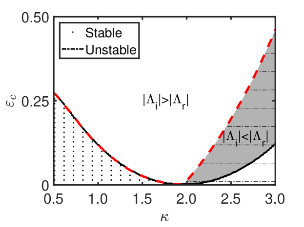
Figure 1: Critical value of $\varepsilon_{c}$ as a function of $\kappa$ is depicted with a red dashed line. In the region above this curve, the necessary condition for stability $|\Lambda_{i}|>|\Lambda_{r}|$ holds. Black solid line (overimposing with red dashed line for $\kappa<2$) represents the values of $\tilde{\varepsilon}$ versus $\kappa$ for which a quadruplet emerges. The dotted region is stable since $\Lambda_{r}=0$. In the dot-dashed region the necessary condition for stability is not satisfied and the solution is unstable. Parameters: $L=50$ and $N=501$.

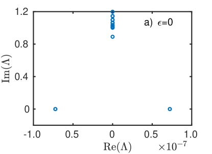
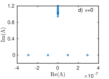
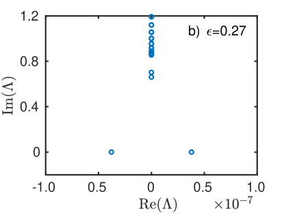
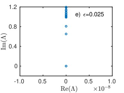
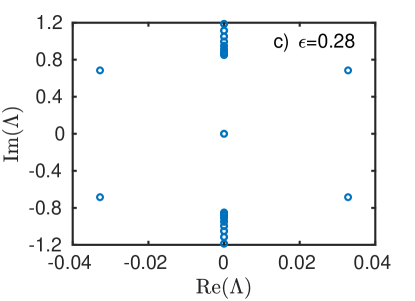
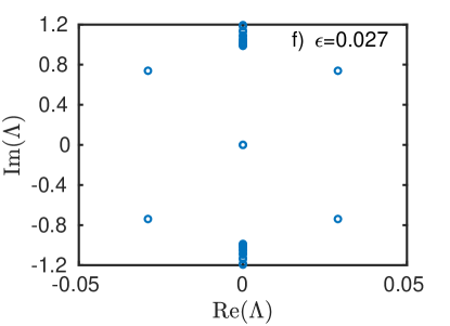
Figure 2: Crucial eigenvalues illustrating the emergence of complex quadruplet as $\varepsilon$ increases. Left-hand side panel: $\kappa=0.5$ ($\varepsilon_{c}=0.273$). For $\varepsilon=0$, the four eigenvalues near to zero are $(\pm 7.23\pm 8.62\,i)\times 10^{-8}$, which approach zero as $N$ increases. Right-hand side panel: $\kappa=1.5$ ($\varepsilon_{c}=0.0268$). Parameters: $L=50$ and $N=1001$.

For each value of $\kappa$, the soliton is stable for the parameters $(\rho,r)$ that lie in the region to the right-hand side of the traveled stability curve $r(\rho)$. Otherwise, it is unstable. These curves monotonically increase with the damping coefficient, except for some values of $\kappa<1$. For instance, for the case of $\kappa=0.5$ shown in Fig. 3 the monotonicity changes. The monotonicity of these curves is related to the motion of the quadruplet as $\varepsilon\geq\varepsilon_{c}$ is increased. In supplemental videos [24], a comparison of the quadruplet’s motion for $\kappa=1.5$ and $\kappa=0.5$ reveals that in the former case, the eigenvalues move apart as $\varepsilon$ is increased, and we move along the curve. In contrast, for $\kappa=0.5$, this behavior is initially observed; however, after a certain value of $\varepsilon$, the 4 eigenvalues begin to attract each other. The parameters used in the simulations depicted in the videos are $L=50$, $N=501$, and the Jacobian is computed only during the first iteration, since it becomes singular very quickly for $\kappa<1$.

Another interesting consequence of the change in monotonicity is the stabilization of the soliton as $r$ increases. Specifically, for $\kappa=0.5$, and a fixed damping coefficient $\rho=0.09$, we observe that for $r=0.27$ the soliton is unstable; however as the amplitude of the parametric force is increased to $r=0.4$, the soliton recovers its stability.

Stability diagrams in Fig. 3 show how the stability can be controlled by the nonlinearity parameter $\kappa$. Generally, it can be achieved by decreasing $\kappa$. Indeed, moving from region A to B, then to C, and finally to D, we find that on region A, the stationary solution is stable for $\kappa=0.5,1.0,1.5,1.75$. On region B, the solution is stable for $\kappa=0.5,1.0,1.5$ and unstable for $\kappa=1.75$. On region C, it is stable for $\kappa=0.5,1.0$ and unstable for $\kappa=1.5,1.75$. Finally, on region D, stability takes place when $\kappa=0.5$.

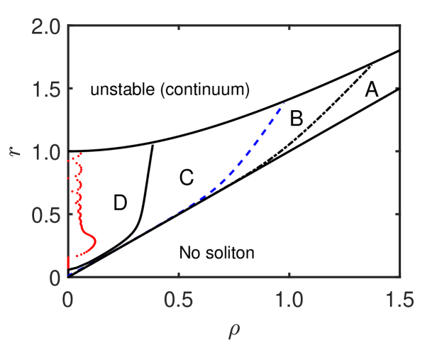
Figure 3: The stability curves, traveled from the lower to the upper boundaries as $\varepsilon$ increases ($\varepsilon_{c}\leq\varepsilon\leq 1$), are depicted for several values of $\kappa<2$: a red dotted line for $\kappa=0.5$, a black solid line for $\kappa=1$, a blue dashed line for $\kappa=1.5$, and a dot-dashed black line for $\kappa=1.75$. These curves are bounded below by $r=\rho$ and above by $r=\sqrt{1+\rho^{2}}$, both represented by black solid lines. For each value of $\kappa$, the soliton is stable when the point $(\rho,r)$ lie on the region to the right-hand side of the corresponding curve. Otherwise, it is deemed unstable. Parameters: $L=50$ and $N=501$.

4.2 $\kappa\geq 2$

For $\varepsilon=0$ we recover the NLS equation with nonlinearity parameter $\kappa$. It is well known that for $\kappa\geq 2$, the stationary NLS solution suffers a blowup of the wave amplitude and becomes unstable [25]. Here, we numerically investigate whether the additional parametric force and damping can stabilize $\Psi_{+}(x,t)$. We employ the same numerical schemes, and solve the discrete versions of Eq. (24) and eigenvalue problem (31)–(32), but now setting $2\leq\kappa\leq 3$.

Fixing $\kappa$, when $\varepsilon$ is increased, we numerically identify in the spectrum four eigenvalues of order $O(10^{-6})$, and other pair of real eigenvalues $\Lambda=\pm\Lambda_{r}$. Therefore, the solitary wave is unstable (see the dot-dashed region below the black solid line in Fig. 1). As $\varepsilon$ increases the real eigenvalues move to zero and two zero eigenvalues move toward them until they collapse and a complex quadruplet arises at $\varepsilon=\tilde{\varepsilon}$ (see the black solid line in Fig. 1). In Fig. 4, for $\kappa=2.5$, is represented the formation of complex quadruplet at $\varepsilon=\tilde{\varepsilon}$, where the dashed line bifurcates in two branches. In the interval $\tilde{\varepsilon}\leq\varepsilon<\varepsilon_{c}$ the solution remains unstable since $|\Lambda_{i}|<|\Lambda_{r}|$ (this condition holds for $\kappa\geq 2$ and defines the shadow and dot-dashed region represented between the black solid line and red dashed line in Fig. 1). For more details, see also a video in the supplementary material [24]. At $\varepsilon=\varepsilon_{c}\approx 0.2$, $\Lambda_{r}=\Lambda_{i}$ (see the intersection between the solid and dashed lines in Fig. 4). A further increment of $\varepsilon$ beyond $\varepsilon_{c}$ leads to the condition $|\Lambda_{i}|>|\Lambda_{r}|$ and to the stability curve. In Fig. 5 the stability curves for $\kappa=2$ and $\kappa=2.5$ are shown. Notice that the curve for $\kappa=2.5$ has two branches, and it is traveled from the lower branch to the upper branch. This indicates that the soliton is stable in the region between these two branches.

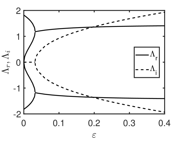
Figure 4: For $\kappa=2.5$, the real and imaginary parts of the eigenvalues which determine the soliton stability are represented as a function of $\varepsilon$. Parameters: $L=50$ and $N=501$.

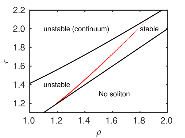
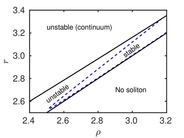
Figure 5: The stability curves are depicted for $\kappa=2$ (red dotted line in the upper panel) and $\kappa=2.5$ (blue dashed line in the lower panel). The curves are bounded below by $r=\rho$ and above by $r=\sqrt{1+\rho^{2}}$, both represented by black solid lines. For each value of $\kappa$, the soliton is stable when the point $(\rho,r)$ lies in the region to the right-hand side of the corresponding traveled curve. Otherwise, it is deemed unstable. Parameters: $L=50$ and $N=501$.

5 Summary

We have investigated the parametrically driven, damped nonlinear Schrödinger equation with an arbitrary nonlinearity parameter $\kappa>0$, focusing on the control of stability through nonlinearity. Two exact stationary solutions, $\Psi_{\pm}(x,t)$, were found. These solutions exist when their frequency is locked to half of the parametric force’s frequency. They are constrained by specific phase conditions, determined by the damping coefficient $\rho$ and by the amplitude $r$ of the parametric force. These conditions are independent of $\kappa$.

The linear stability of these waves was examined by linearizing the parametrically, driven NLS equation around $\Psi_{\pm}(x,t)$. This approach leads to a separation of variables, resulting in a Sturm-Liouville problem (SLP) that depends on the parameters $r$, $\rho$ and $\kappa$. Consequently, there are three ways to modify the spectrum of this problem and thus its stability: varying $r$, modifying $\rho$, and by adjusting the additional parameter $\kappa$.

The presence of these multiple parameters enriches the analysis while complicating the resolution of the problem. A special parametrization through $\varepsilon=\varepsilon_{\pm}$ provides an efficient and precise method for determining the stability. For $\Psi_{-}(x,t)$, where $\varepsilon_{-}\in(-\infty,0)$, we analytically demonstrate that the spectrum of SLP contains a real positive eigenvalue, indicating that the solution is unstable for all values of $\kappa$.

Conversely, for $\Psi_{+}(x,t)$, where $\varepsilon_{+}\in[0,1]$, the SLP is numerically solved. Our primary findings are as follows: i) for $0.25\leq\kappa<2$, there exists a critical value of $\varepsilon_{c}$ such that when $\varepsilon_{+}<\varepsilon_{c}$, the spectrum contains numerically close to zero and pure imaginary eigenvalues, indicating that the soliton is stable. For $\kappa=1$ the results obtained in Ref. [1] are recovered. ii) As $\varepsilon_{+}$ increases, the internal mode and a detached mode from zero move toward each other along the imaginary axis. At the critical value $\varepsilon_{+}=\varepsilon_{c}$, they collapse, leading to the formation of a quadruplet $\{\Lambda,-\Lambda,\Lambda^{\star},-\Lambda^{\star}\}$, $\Lambda=\Lambda_{r}+i\Lambda_{i}$ with a repulsion among their eigenvalues. iii) We demonstrate that $|\Lambda_{i}|>|\Lambda_{r}|$ when $\kappa<2$. As a consequence, is obtained a family of $\kappa$-stability curve, $r(\rho)$, which defines the boundary between the unstable and stable regions. This mechanism resembles the oscillatory instability observed when $\kappa=1$, where the role of the internal mode is taken over by a mode that has separated from the continuum spectrum [1]. iv) We investigate several cases in detail, specifically for $\kappa<1$, and $1<\kappa<2$. In the former case, the monotonicity of the curves $r(\rho)$ undergoes a change owing to the attraction of a complex quadruplet toward the continuum spectrum.

Additionally, we numerically assess the stability of $\Psi_{+}(x,t)$ for $2\leq\kappa\leq 3$. For $\varepsilon_{+}=0$, the soliton is unstable due to the presence of a pair of nonzero real eigenvalues in the spectrum, consistent with previous studies on amplitude blowup in the NLS equation [25]. As $\varepsilon_{+}$ increases, this pair of eigenvalues moves toward zero, while another pair moves away from zero toward them. The collision of these eigenvalues occurs in the real axis. Although a complex quadruplet emerges, the soliton remains unstable since $|\Lambda_{i}|\leq|\Lambda_{r}|$. Solely when $\varepsilon_{+}>\varepsilon_{c}$ and $|\Lambda_{i}|>|\Lambda_{r}|$ a stability region arises.

In conclusion, the parametric force stabilizes the damped soliton, even for $\kappa\geq 2$ where oscillatory stability is observed; however, it simultaneously breaks Galilean invariance, preventing the derivation of moving solitons from stationary solutions. Future work may focus on analyzing the existence and stability of moving solitons in the parametrically driven, damped nonlinear Schrödinger equation with arbitrary nonlinearity parameter.

Appendix A $\Psi_{-}(X)$ is unstable

Here we proof that $\Psi_{-}(X)$ given by Eq. (15) is always unstable solution regardless of the value of $\kappa>0$. In order to consider this solution we assume $\varepsilon=\varepsilon_{-}<0$. For $\kappa=1$ this was proved in Ref.[26]. We will need the following two propositions:

Proposition A1: For any $\varepsilon$ and $\kappa>0$, $L_{1}$ possesses a zero eigenvalue associated with the eigenfunction $\psi_{X}(X)$, which implies that $L_{1}$ also has always a negative eigenvalue associated to a nodeless eigenfunction, $\psi_{0}(X)$.

Proof: From Eqs. (23) and (24) follows that $L_{1}\psi_{X}=0$. This implies that $\psi_{X}(X)$ is an eigenfunction of $L_{1}$ associated to the zero eigenvalue. Since $L_{1}$ is a Sturm-Liouville operator, its eigenvalues are ordered in increasing magnitude (see e.g. Ref. [27, page 722]), corresponding to the number of nodes in their respective eigenfunctions. This implies that if $\psi_{X}(X)$ has one node, then there exists a nodeless eigenfunction, $\psi_{0}(X)$, associated to a negative eigenvalue. $\Box$

Proposition A2: $L_{0}$ is strictly positive defined for $\varepsilon<0$.

Proof: From Eq. (24) it follows that $L_{0}\psi=-\varepsilon\psi$. Because $\psi(X)$ is a nodeless function, their corresponding eigenvalue $-\varepsilon$ is the lowest one (see e.g. [27, page 722]). Since $\varepsilon<0$, then the lowest eigenvalue is positive, and then the others eigenvalues are also positive. Moreover, for the continuous spectrum of $L_{0}$, $\sigma_{c}(L_{0})\subset[\sqrt{1-\varepsilon},+\infty)$. Therefore, by Theorem 2.18 of [28], for $\varepsilon<0$, $L_{0}$ is strictly positive defined operator. $\Box$

Since the operator $L_{0}$ is positive definite (Proposition A2) and therefore invertible, then the system (31)–(32) can be rewritten as

$$L_{1}f_{c}=-\Lambda^{2}L_{0}^{-1}f_{c}.$$ (39)

Thus

$$\Lambda^{2}=-\frac{\langle f_{c}|L_{1}f_{c}\rangle}{\langle f_{c}|L_{0}^{-1}f_{c}\rangle}.$$ (40)

Let us now define the functional $\Sigma:H^{1}(\mathbb{C})\to\mathbb{R}$ as

$$\Sigma(\xi)=-\frac{\langle\xi|L_{1}\xi\rangle}{\langle\xi|L_{0}^{-1}\xi\rangle},$$ (41)

where $H^{1}(\mathbb{C}):=\{\xi\in L^{2}(\mathbb{C}),\partial\xi\in L^{2}(\mathbb{C})\}$, where $\partial$ denotes the weak derivative. Since $L_{0}$ is strictly positive definite, the denominator of the functional $\Sigma$ given in Eq. (41) does not vanished, and since $L_{0}$ and $L_{1}$ are hermitian operators, the functional is well defined.

Let $\Lambda_{0}^{2}$ be

$$\Lambda_{0}^{2}=\max_{\xi}\Sigma(\xi).$$ (42)

Taking into account that $\Sigma(\psi_{0}(X))>0$, where $\psi_{0}(X)$ is the fundamental eigenfunction of $L_{1}$ (Proposition A1), we obtain that $\Lambda_{0}^{2}>0$.

The next step is to verify if $\Lambda_{0}^{2}$ is an eigenvalue of Eq. (39). Let’s denote as $\xi_{0}$ the function where $\Sigma(\xi_{0})=\Lambda_{0}^{2}$, and choose $\alpha\in\mathbb{R}$ and $h\in H^{1}(\mathbb{C})$.

Since the functional $\Sigma$ attains its maximum at $\xi_{0}$, then we have that

$$0=\left.\frac{d}{d\alpha}\Sigma(\xi_{0}+\alpha h)\right|_{\alpha=0}=-\frac{\left(\langle h|L_{1}\xi_{0}\rangle+\langle\xi_{0}|L_{1}h\rangle\right)\langle\xi_{0}|L_{0}^{-1}\xi_{0}\rangle-\langle\xi_{0}|L_{1}\xi_{0}\rangle\left(\langle h|L_{0}^{-1}\xi_{0}\rangle+\langle\xi_{0}|L_{0}^{-1}h\rangle\right)}{\langle\xi_{0}|L_{0}^{-1}\xi_{0}\rangle^{2}},$$

and thus

$$0= \left(\langle h|L_{1}\xi_{0}\rangle+\langle\xi_{0}|L_{1}h\rangle\right)+\Lambda_{0}^{2}\left(\langle h|L_{0}^{-1}\xi_{0}\rangle+\langle\xi_{0}|L_{0}^{-1}h\rangle\right)$$

$$= \langle h|\left(L_{1}+\Lambda_{0}^{2}L_{0}^{-1}\right)\xi_{0}\rangle+\langle\xi_{0}|\left(L_{1}+\Lambda_{0}^{2}L_{0}^{-1}\right)h\rangle$$

$$= \langle h|\left(L_{1}+\Lambda_{0}^{2}L_{0}^{-1}\right)\xi_{0}\rangle+\langle h|\left(L_{1}+\Lambda_{0}^{2}L_{0}^{-1}\right)\xi_{0}\rangle^{*}=2\real\langle h|\left(L_{1}+\Lambda_{0}^{2}L_{0}^{-1}\right)\xi_{0}\rangle.$$

Because $h$ is any function in the space, we deduce that

$$\left(L_{1}+\Lambda_{0}^{2}L_{0}^{-1}\right)\xi_{0}=0,$$ (43)

which proofs that $\Lambda_{0}^{2}>0$ satisfies Eq. (39).

This implies that there exists $\Lambda_{0}\in\mathbb{R}^{+}$ in the spectrum of the system (31)–(32), and so we have that for $\varepsilon<0$, the solution $\psi_{-}(X)$ is always unstable.

Appendix B $|\Lambda_{i}|>|\Lambda_{r}|$ for $\kappa<2$

In the resolution of the eigenvalue problem corresponding to the stability analysis of $\Psi_{+}(x,t)$, when $\varepsilon\in[\tilde{\varepsilon},1]$, $\tilde{\varepsilon}>0$, appear four complex eigenvalues $\{\Lambda,-\Lambda,\Lambda^{\star},-\Lambda^{\star}\}$, being $\Lambda=\Lambda_{r}+i\Lambda_{i}$. Here, we will prove that if $\kappa<2$, then $|\Lambda_{i}|>|\Lambda_{r}|$. This implies that $\tilde{\varepsilon}=\varepsilon_{c}$ for $\kappa<2$, where $\varepsilon_{c}$ is the threshold value for the emergence of quadruplet.

Let us consider the operator $\widetilde{L}_{0}=L_{0}+\varepsilon$, where $L_{0}$ is defined by Eq. (22) and $\widetilde{L}_{0}$ satisfies

$$\widetilde{L}_{0}\psi=\left(L_{1}+2\kappa(2-\varepsilon)\psi^{2\kappa}\right)\psi=0.$$ (44)

Next, we will consider the following functions

$$f_{c}=\beta\psi+\bar{f},\qquad\widetilde{g}_{c}=\alpha\psi+\bar{g},$$ (45)

where both $\bar{g}$ and $\bar{f}$ are orthogonal to $\psi$, and $\alpha,\beta\in\mathbb{C}$. Inserting them into the system (31)–(32), we obtain

$$\widetilde{L}_{0}\bar{g}-\varepsilon\bar{g} =(\varepsilon\alpha+\beta\Lambda)\psi+\Lambda\bar{f},$$ (46)

$${L}_{1}\bar{f}+L_{1}\beta\psi =-\Lambda\alpha\psi-\Lambda\bar{g}.$$ (47)

Multiplying Eq. (46) by $\psi$ and integrating over $\mathbb{R}$ we get

$$\begin{split}\langle\psi|\widetilde{L}_{0}\bar{g}\rangle-\varepsilon\langle\psi|\bar{g}\rangle=(\varepsilon\alpha+\beta\Lambda)\langle\psi|\psi\rangle+\Lambda\langle\psi|\bar{f}\rangle,\end{split}$$ (48)

from where, taking into account that $\langle\psi|\widetilde{L}_{0}\bar{g}\rangle=\langle\widetilde{L}_{0}\psi|\bar{g}\rangle=0$, Eq. (44), as well as the orthogonality of $\bar{g}$ and $\bar{f}$ with respect to $\psi$, we find the relation $\varepsilon\alpha=-\beta\Lambda$. Using this relation the Eq. (46) becomes

$$\widetilde{L}_{0}\bar{g}-\varepsilon\bar{g} =\Lambda\bar{f}.$$ (49)

Now we multiply the Eq. (49) by $\bar{g}$ and integrate over $\mathbb{R}$ to get

$$\langle\bar{g}|\widetilde{L}_{0}\bar{g}\rangle-\varepsilon\innerproduct{\bar{g}}{\bar{g}}=\Lambda\innerproduct{\bar{g}}{\bar{f}}.$$ (50)

Since $\widetilde{L}_{0}$ is self-adjoint then $\langle\bar{g}|\widetilde{L}_{0}\bar{g}\rangle$ is real, therefore from (50) it follows that $\Lambda\innerproduct{\bar{g}}{\bar{f}}$ is also real, i.e., $(\Lambda\innerproduct{\bar{g}}{\bar{f}})^{\star}=\Lambda\innerproduct{\bar{g}}{\bar{f}}$. From the last condition and after some straightforward calculations we deduce that there exists $\gamma\in\mathbb{R}$ such that

$$\innerproduct{\bar{g}}{\bar{f}}=\gamma{\Lambda}^{\star}.$$ (51)

Now we multiply Eq. (47) by $\bar{f}$ and integrate over $\mathbb{R}$, to obtain

$$\langle\bar{f}|{L}_{1}\bar{f}\rangle+\beta\langle\bar{f}|L_{1}\psi\rangle =-\Lambda\langle\bar{f}|\bar{g}\rangle.$$ (52)

Taking the complex conjugation in the last equation and using relation (51) it transforms into

$$\langle\bar{f}|{L}_{1}\bar{f}\rangle+\beta^{\star}\langle\psi|L_{1}\bar{f}\rangle=-\gamma\left(\Lambda^{\star}\right)^{2}.$$ (53)

Next we multiply Eq. (47) by $\psi$ and integrate over $\mathbb{R}$ to get

$$\langle\psi|{L}_{1}\bar{f}\rangle+\beta\langle\psi|L_{1}\psi\rangle =-\Lambda\alpha\langle\psi|\psi\rangle.$$ (54)

Subtracting the Eq. (53) to the Eq. (54) multiplied by $\beta^{\star}$, and using that $\alpha=-\Lambda\beta/\varepsilon$, we obtain

$$\begin{split}\langle\bar{f}|{L}_{1}\bar{f}\rangle-|\beta|^{2}\langle\psi|L_{1}\psi\rangle=-\gamma\left(\Lambda^{\star}\right)^{2}-|\beta|^{2}\Lambda^{2}\frac{\langle\psi|\psi\rangle}{\varepsilon}.\end{split}$$ (55)

Since $L_{1}$ is self-adjoint, the left hand side of (55) is real. Therefore,

$$\begin{split}\imaginary\left(-\gamma\left(\Lambda^{\star}\right)^{2}-|\beta|^{2}\Lambda^{2}\frac{\langle\psi|\psi\rangle}{\varepsilon}\right)=0.\end{split}$$ (56)

Now, we notice that when the quadruplet is formed, $\Lambda_{i},\Lambda_{r}\neq 0$, then

$$\gamma=|\beta|^{2}\frac{\langle\psi|\psi\rangle}{\varepsilon}.$$ (57)

Substituting Eq. (57) into Eq. (55), yields

$$\begin{split}\langle\bar{f}|{L}_{1}\bar{f}\rangle-|\beta|^{2}\langle\psi|L_{1}\psi\rangle=\left(\Lambda_{i}^{2}-\Lambda_{r}^{2}\right)|\beta|^{2}\frac{\langle\psi|\psi\rangle}{\varepsilon}.\end{split}$$ (58)

We will show that, for $\beta\neq 0$, the left-hand side of (58) is positive, therefore, $\Lambda_{i}^{2}>\Lambda_{r}^{2}$. First, from Eq. (44) follows

$$\langle\psi|L_{1}\psi\rangle=-2\kappa(2-\varepsilon)\int_{\mathbb{R}}\psi^{2\kappa+2}\,dx<0.$$ (59)

Next we prove that $\langle\bar{f}|{L}_{1}\bar{f}\rangle\geq 0$. For doing that we use the following result (see Proposition 2.7 of Ref. [29, pag. 477]):

Proposition B1: $L_{1}$ verifies for $\kappa<2$ that

$$\inf_{\innerproduct{\xi}{\psi}=0}\innerproduct{\xi}{L_{1}\xi}=0.$$ (60)

In other words, for $\kappa<2$, $\innerproduct{\xi}{L_{1}\xi}\geq 0$ for all $\xi$ orthogonal to $\psi$, i.e., $L_{1}$ is positive definite in the subspace orthogonal to $\psi$. Combining this two results it follows that $\Lambda_{i}^{2}>\Lambda_{r}^{2}$ for any quadruplet obtained when $\kappa<2$, and therefore the dotted black line and the dashed red line in Fig. 1 are indeed identical for $\kappa<2$.

Finally, we show that necessarily $\beta\neq 0$. Indeed, if $\beta=0$, then, according to Eq. (58), $\langle\bar{f}|{L}_{1}\bar{f}\rangle=0$. Moreover, in this case $\alpha=0$, $\bar{f}=f_{c}$ and $\bar{g}=\widetilde{g}_{c}$. So the infimum in Eq. (60) is attained when $\xi=f_{c}$, therefore, for any $h$

$$0=\left.\frac{d}{d\alpha}\innerproduct{f_{c}+\alpha h}{L_{1}(f_{c}+\alpha h)}\right|_{\alpha=0}=2\real\innerproduct{h}{L_{1}f_{c}}.$$

Thus, $L_{1}f_{c}=0$. Using that the Eq. (47), for this case, reads $L_{1}f_{c}=-\Lambda\widetilde{g}_{c}$, it follows that $\widetilde{g}_{c}=0$, and Eq. (49) yields $f_{c}=0$, which is a contradiction.

Acknowledgments

We thanks Ricardo Carretero for sending us a preliminary version of Ref. [20] and Igor Barashenkov for drawing the Ref. [26] to our attention. F.C.N. acknowledges financial support through the Programa de Iniciación a la Investigación PI3 (IMUS) and hospitality at IMUS (University of Seville). R.A.N. was partially supported by PID2021-124332NB-C21 (FEDER(EU)/Ministerio de Ciencia e Innovación-Agencia Estatal de Investigación, Spain) and FQM-415 (Junta de Andalucía, Spain). N.R.Q. was partially supported by the Spanish projects PID2020-113390GB-I00 (MICIN), and FQM-415 (Junta de Andalucía, Spain).

References

- [1] I. V. Barashenkov, M. M. Bogdan, and V. I. Korobov. Stability Diagram of the Phase-Locked Solitons in the Parametrically Driven, Damped Nonlinear Schrödinger Equation. Europhys. Lett., 15:113, 1991.
- [2] M. Bondila, I. V. Barashenkov, and M. M. Bogdan. Topography of attractors of the parametrically driven nonlinear Schrödinger equation. Physica D, 87:314, 1995.
- [3] X. Wang and R. Wei. Interactions and motions of double-solitons with opposite polarity in a parametrically driven system. Phys. Lett. A, 227:55, 1997.
- [4] W. Wang, X. Wang, J. Wang, and R. Wei. Dynamical behavior of parametrically excited solitary waves in Faraday’s water trough experiment. Phys. Lett. A, 219:74, 1996.
- [5] X. Wang and R. Wei. Oscillatory patterns composed of the parametrically excited surface-wave solitons. Phys. Rev. E, 57:2405, 1998.
- [6] L. Gordillo and M. A. García-Ñustes. Dissipation-driven behavior of nonpropagating hydrodynamic solitons under confinement. Phys. Rev. Lett., 112:164101, 2014.
- [7] I. V. Barashenkov and E. V. Zemlyanaya and M. Bär. Traveling solitons in the parametrically driven nonlinear Schrödinger equation. Phys. Rev. E, 64:016603, 2001.
- [8] F. G. Mertens and N. R. Quintero. Empirical stability criteria for parametrically driven solitons of the nonlinear Schrödinger equation. J. Phys. A: Math. Gen., 53:315701, 2020.
- [9] X. Wang. Parametrically excited nonlinear waves and their localizations. Phys. D: Nonlinear Phenom., 154:337, 2001.
- [10] M. M. Bogdan and O. V. Charkina. Structure of soliton bound states in the parametrically driven and damped nonlinear systems. Low Temp. Phys., 48:1062, 2022.
- [11] J. M. Miles. Parametrically excited solitary waves. J. Fluid Mech, 148:451, 1984.
- [12] A. Scott. Nonlinear Science: Emergence and Dynamics of Coherent Structures, Oxford Texts in Applied and Engineering Mathematics, Vol. 8. Oxford University Press, 2003.
- [13] T. Dauxois and M. Peyrard. Physics of Solitons. Cambridge University Press, 2010.
- [14] A. Sánchez and A. R. Bishop. Collective coordinates and length-scale competition in spatially inhomogeneous soliton-bearing equations. SIAM Rev., 40:579, 1998.
- [15] M. M. Bogdan, A. M. Kosevich, and I. V. Manzhos. Stabilization of a magnetic soliton (bion) as a result of parametric excitation of one-dimensional ferromagnet. Fiz. Niz. Temp., 11:991, 1985.
- [16] N. V. Alexeeva, I. V. Barashenkov, and D. E. Pelinovsky. Nonlinearity, 12:103, 1999.
- [17] F. Cooper, A. Khare, A. Comech, B. Mihaila, J. F. Dawson, and A. Saxena. Stability of exact solutions of the nonlinear Schrödinger equation in an external potential having supersymmetry and parity-time symmetry. J. Phys. A: Math. Gen., 50:015301, 2016.
- [18] M. Bondila, I. V. Barashenkov, and M. M. Bogdan. Topography of attractors of the parametrically driven nonlinear Schrödinger Equation. Physica D, 87:314, 1995.
- [19] W. H. Press, S. A. Teukolsky, W. T. Vetterling, and B. P. Flannery. Numerical Recipes in FORTRAN: the Art of Scientific Computing. Cambridge: Cambridge University Press, 1992.
- [20] R. Carretero-González, D.J. Frantzeskakis, and P.G. Kevrekidis. Nonlinear Waves & Hamiltonian Systems: From One To Many Degrees of Freedom, From Discrete To Continuum. Oxford University Press, 2024.
- [21] J.M. Ortega and W.C. Rheinboldt. Chapter 7 - general iterative methods. In J.M. Ortega and W.C. Rheinboldt, editors, Iterative Solution of Nonlinear Equations in Several Variables, pages 181–239. Academic Press, 1970.
- [22] M. Y. Waziri, W. J. Leong, M. A. Hassan, and M. Monsi. An Efficient Solver for Systems of Nonlinear Equations with Singular Jacobian via Diagonal Updating. Appl. Math. Sci., 4:3403, 2010.
- [23] Matlab, The Language of Technical Computing. Math Works, Inc., Natick, MA, 2020.
- [24] See Supplemental Material for movies showing the evolution of crucial eigenvalues for as increases.
- [25] C. Sulem and C. L. Sulem. The Nonlinear Schrödinger Equation. New York: Springer, 1999.
- [26] I. V. Barashenkov, T. Zhanlav, and M. M. Bogdan. in Nonlinear World. IV International Workshop on Nonlinear and Turbulent Processes in Physics. World Scientific, Kiev, 9-22 October 1989, 1990.
- [27] P. M. Morse and H. Feshbach. Methods of Theoretical Physics, volume 1. McGraw-Hill, New York, 1953.
- [28] G. Teschl. Mathematical Methods in Quantum Mechanics: With Applications to Schrödinger Operators. Graduate Studies in Mathematics, 99. American Mathematical Society, Providence, R.I., 2009.
- [29] M. I. Weinstein. Modulational Stability of Ground States of Nonlinear Schrödinger Equations. SIAM J. Math. Anal., 16:472, 1985.