Could the neutrino emission of TXS 0506+056 come from the accretion flow of the supermassive black hole?

Abstract

High-energy neutrinos from the blazar TXS 0506+056 are usually thought to arise from the relativistic jet pointing to us. However, the composition of jets of active galactic nuclei (AGNs), whether they are baryon dominated or Poynting flux dominated, is largely unknown. In the latter case, no comic rays and neutrinos are expected from the AGN jets. In this work, we study whether the neutrino emission from TXS 0506+056 could be powered by the accretion flow of the supermassive black hole. Protons could be accelerated by magnetic reconnection or turbulence in the inner accretion flow. To explain the neutrino flare of TXS 0506+056 in the year of 2014-2015, a super-Eddington accretion is needed. During the steady state, a sub-Eddington accretion flow could power a steady neutrino emission that may explain the long-term neutrino flux from TXS 0506+056. We consider the neutrino production in both magnetically arrested accretion (MAD) flow and the standard and normal evolution (SANE) regime of accretion. In the MAD scenario, due to a high magnetic field, a large dissipation radius is required to avoid the cooling of protons due to the synchrotron emission.

1 Introduction

Active Galactic Nuclei (AGN) are prime candidate sources of the high-energy astrophysical neutrinos. In 2017, IceCube detected a high-energy neutrino event in the direction coincident with the blazar TXS 0506+056, which was found to be flaring at the gamma-ray band (IceCube Collaboration et al., 2018a). A follow-up analysis of archival IceCube neutrino data revealed an earlier outburst of neutrinos from the same source in 2014/2015 without an accompanying flare of gamma rays(IceCube Collaboration et al., 2018b). Later, an independent search for point-like sources in the northern hemisphere using ten years of IceCube data revealed that TXS 0506+056 is coincident with the second hottest-spot of the neutrino event excess (IceCube Collaboration et al., 2022). Since blazars are AGNs with relativistic jets pointing toward our line of sight, the Doppler effect remarkably boosts the flux of blazars received by us. Most of the previous studies ascribe the high-energy neutrino emission of TXS 0506+056 to relativistic protons accelerated in the jet, through either photopion production with the radiation of the jet itself and the external radiation of the surrounding environment (e.g. Murase et al., 2018; Keivani et al., 2018; Gao et al., 2019; Cerruti et al., 2019; Rodrigues et al., 2019; Xue et al., 2019; Zhang et al., 2020; Xue et al., 2021) , or proton-proton collisions with matter of the jet and cloud/star entering the jet (e.g. Sahakyan, 2018; Liu et al., 2019; Banik et al., 2020; Wang et al., 2022) .

IceCube Collaboration et al. (2022) reported an excess of neutrino events associated with NGC 1068, a nearby type-2 Seyfert galaxy , with a significance of 4.2$\sigma$. Seyfert galaxies are radio-quiet AGNs with much weaker jets compared to blazars. In NGC 1068, a supermassive black hole (SMBH) at the center is highly obscured by thick gas and dust (Gámez Rosas et al., 2022). X-ray studies have suggested that NGC 1068 is among the brightest AGNs in intrinsic X-rays (Bauer et al., 2015), which is generated through Comptonization of accretion-disk photons in hot plasma above the accretion disk, namely the coronae. Given the dense matter and the intense radiation in the environment, efficient neutrino production is expected if cosmic rays are accelerated at the proximity of the SMBH (Murase et al., 2020a; Inoue et al., 2020). Interestingly, the reported neutrino flux is higher than the GeV gamma-ray flux, implying that gamma-rays above 100 MeV are strongly attenuated by dense X-ray photons while neutrinos can escape.

A correlation between unabsorbed hard X-rays and neutrinos in radio-loud and radio-quiet AGN is suggested by Kun et al. (2024), raising the possibility of a common neutrino production mechanism involved in both types of AGNs. Since neutrino emission from radio-quiet Seyfert galaxies is unlikely related to their weak jets, a natural question arises as to whether neutrinos from blazars can be produced somewhere besides their powerful jets, such as from the proximity of the SMBH.

Hadronic interactions responsible for the neutrino production also generate gamma rays with comparable flux and energy spectra to that of neutrinos. If such interactions take place near the SMBH, where intense infrared-optical photons from the accretion disk and X-rays from the hot corona are present, pair production and subsequent electromagnetic cascade will reprocess the gamma rays into keV-MeV photons. The apparent underproduction of gamma-rays compared to neutrinos in Seyfert galaxies is naturally explained in such environments. A hint of strong gamma-absorption in neutrino sources is also observed in the diffuse neutrino flux (Murase et al., 2020b), pointing to the so-called "hidden" neutrino sources. Motivated by the above reasoning, in this paper, we investigate the possibility that the steady neutrino emission and the neutrino outburst of TXS 0506+056 are produced by the core region of the AGN. Indeed, there have been suggestions that particles may be accelerated in the accretion disk via magnetic reconnection and turbulence (e.g. Yuan et al., 2003; de Gouveia Dal Pino et al., 2010; Hoshino, 2013; Kunz et al., 2016; Ripperda et al., 2022; Kheirandish et al., 2021). If the SMBH has a fast-rotating magnetosphere, the centrifugal force may also serve as an efficient particle accelerator(Gangadhara & Lesch, 1997; Rieger & Aharonian, 2008).

The rest part of the paper is organized as follows. We introduce our model in Section 2 and show the results in Section 3. We discuss and summarize the results in Section 4.

2 Neutrinos from the AGN disk in TXS 0506+056 ?

The blazar TXS 0506+056 is the first individual neutrino source identified at $>3\sigma$ significance excess and $13\pm 5$ high-energy neutrino events was discovered in the period between September 2014 and March 2015. (IceCube Collaboration et al., 2018b). For this period, the neutrino integrated luminosity (per flavor) between 32 TeV and 4 PeV is estimated to be $L_{\nu_{\mu}}\sim 10^{47}\rm{erg~{}s^{-1}}$. The time-integrated analysis of the ten years of IceCube data revealed that TXS 0506+056 is coincident with the second hottest-spot of the neutrino event excess (IceCube Collaboration et al., 2022). A mean flux of $\sim 10^{-13}{\rm TeVcm^{-2}s^{-1}}$ is obtained (IceCube Collaboration et al., 2022), corresponding to a neutrino luminosity of $L_{\nu_{\mu}}\sim 5\times 10^{44}\rm{erg~{}s^{-1}}$.

The Eddington luminosity of the accretion disk in TXS 0506+056 is estimated to be

$$L_{\rm Edd}=4\times 10^{46}{\rm erg~{}s^{-1}}\left(\frac{M_{\rm BH}}{3\times 10^{8}M_{\odot}}\right),$$ (1)

where $M_{\rm BH}$ is the mass of the supermassive black hole. The Eddington accretion rate is defined as $\dot{M}_{\rm Edd}=L_{\rm Edd}/({\eta_{a}}c^{2})$, where $\eta_{a}=0.1$ (Yuan & Narayan, 2014) Assuming an efficiency $\epsilon_{\rm CR}$ for accretion power converted into cosmic rays, the cosmic ray luminosity is estimated to be

$$L_{\rm CR} =\epsilon_{\rm CR}\dot{M}c^{2}$$ (2)

$$=4\times 10^{46}{\rm erg~{}s^{-1}}\left(\frac{\epsilon_{\rm CR}}{0.1}\right)\left(\frac{\dot{m}}{1}\right)\left(\frac{M_{\rm BH}}{3\times 10^{8}M_{\odot}}\right).$$

where $\dot{m}=\dot{M}/\dot{M}_{\rm Edd}$ is the dimensionless accretion rate. Then the neutrino luminosity (per flavor) produced by cosmic rays via $pp$ or $p\gamma$ interaction is given by

$$L_{\rm\nu_{\mu}} =\frac{1}{8}f_{pp,p\gamma}L_{CR}$$ (3)

$$\sim 5\times 10^{45}{\rm erg~{}s^{-1}}\left(\frac{\epsilon_{\rm CR}}{0.1}\right)\left(\frac{\dot{m}}{1}\right)\left(\frac{M_{\rm BH}}{3\times 10^{8}M_{\odot}}\right).$$

Here $f_{pp,p\gamma}=t_{\rm loss}/t_{pp,p\gamma}$ is the efficiency of $pp$ and $p\gamma$ processes expressed in the ratio of the proton energy loss timescale and hadronic interaction timescale, which will be discuss in following sections. To explain the observed neutrino luminosity, we require

$$\dot{m}\sim 20f_{pp,p\gamma}^{-1}\left(\frac{\epsilon_{\rm CR}}{0.1}\right)^{-1}\left(\frac{M_{\rm BH}}{3\times 10^{8}M_{\odot}}\right)^{-1}\left(\frac{L_{\nu_{\mu}}}{10^{47}{\rm ergs^{-1}}}\right)^{-1}.$$ (4)

Therefore, to explain the neutrino flare during 2014-2015, a super-Eddington accretion rate is required. On the other hand, to explain the 10-year quasi-steady-state neutrino emission with a flux 2 orders of magnitude lower, a sub-Eddington accretion may be viable.

2.1 The process of proton acceleration and cooling within the core of TXS 0506+056

As we mentioned above, high-energy protons may be accelerated by magnetic reconnection, stochastic acceleration via MHD turbulence or electric potential gaps in the black hole magnetosphere. We here do not specify the detailed acceleration mechanism, but phenomenologically parameterize the particle acceleration timescale by

$$t_{\rm acc}\approx\frac{\eta r_{\rm L}}{c}$$ (5)

where the different mechanisms may be characterized by distinct parameter $\eta$, which could be understood as the particle acceleration efficiency. $r_{\rm L}=E/eB$ is the Larmor radius. The maximum energy of non-thermal proton is determined by the balance among particle acceleration, cooling, and escape processes in the core region. The escape term is common for all components. We consider diffusion and advection (infall to the BH) as the escape processes, whose timescales are estimated to be $t_{\rm diff}\approx R^{2}/D_{\rm R}$ and $t_{\rm fall}\approx R/V_{\rm R}$ respectively, where $D_{\rm R}=D_{\rm R}\approx\eta r_{\rm L}c/3$ is the diffusion coefficient and $\eta r_{\rm L}$ is the effective mean free path. The total escape time is given by $t_{\rm esc}^{-1}=t_{\rm diff}^{-1}+t_{\rm fall}^{-1}$.

For the cooling of cosmic ray protons, we consider inelastic collisions ($pp$), photomeson production ($p\gamma$), Bethe-Heitler pair production, and proton synchrotron radiation. The photon field includes the multi-temperature black-body emission from the accretion disk and hard X-ray emission from comptonized corona. The coronal spectrum can be modeled by a power law with an exponential cutoff. The photon index of TXS 0506+056, $\Gamma_{X}$, varies between 1.5 – 1.9 among observations (Acciari et al., 2022). The photon index is correlated with $\lambda_{\rm Edd}=L_{\rm bol}/L_{\rm Edd}\sim 0.24$ as $\Gamma_{X}\approx 0.167\times\rm{log}(\lambda_{\rm Edd})+2.0=1.89$ (Trakhtenbrot et al., 2019), and the cutoff energy is given by $\varepsilon_{\rm X,cut}\sim-74\rm{log}(\lambda_{Edd})+1.5\times 10keV=0.19MeV$ (Ricci et al., 2018). We use the average hard X-ray luminosity in 15–55 keV of $(9.0\pm 2.4)\times 10^{44}~{}\rm{erg~{}s^{-1}}$ to normalize the quasi-steady state X-ray component with sub-Eddington accretion (Kun et al., 2024). In the flare state characterized by an accretion rate two orders of magnitude higher, the bolometric luminosity would increase by a factor of 5-6 compared with that in the steady state (Huang et al., 2020).

For the radiation of the disk, we consider a multi-temperature blackbody emission with the maximum temperature near the central supermassive black hole $T_{\text{disk}}\approx 0.49(GM_{\rm BH}\dot{M}/(72\pi\sigma_{\text{SB}}R_{S}^{3}))^{1/4}K$ (Pringle, 1981). The temperature of the disk can be epressed as $T(R)\approx(R/R_{S})^{-3/4}$. Here, $M_{\rm BH}$ is the SMBH mass, $R_{S}=2GM_{\rm BH}/c^{2}$ is the Schwarzschild radius, and $\sigma_{\text{SB}}$ is the Stefan-Boltzmann constant. We can calculate the disk luminosity as

$$L_{\nu}=\frac{8\pi h\nu^{3}}{c^{2}}\int_{R_{S}}^{R}\frac{rdr}{e^{(h\nu/kT(R))}-1}.$$ (6)

The timescale of photomeson process ($p\gamma$) is $t_{p\gamma}\approx 1/(n_{\gamma}\sigma_{p\gamma}\kappa_{p\gamma}c)$, where ${\sigma}_{p\gamma}\approx 5\times 10^{-28}~{}\rm{cm}^{2}$ is the cross section for the photomeson process and $\kappa_{p\gamma}\sim 0.2$ is the inelasticity for $p\gamma$. The Bethe-Heitler energy loss rate is $t_{\rm B-H}\approx 1/(n_{\gamma}\hat{\sigma}_{\rm B-H}c)$, where $\hat{\sigma}_{\rm B-H}\sim 0.8\times 10^{-30}\rm{cm}^{-3}$ is the effective cross section for the Bethe-Heitler process (Murase et al., 2020b). The $pp$ cooling timescale is $t_{pp}\approx 1/(n_{p}{\sigma}_{pp}\kappa_{pp}c)$, where ${\sigma}_{pp}\simeq 4\times 10^{-26}\rm{cm}^{2}$ and $\kappa_{\rm pp}\approx 0.5$ are cross section and inelasticity for $pp$ process (Kelner et al., 2006). The proton synchrotron timescale is $t_{p,\rm{syn}}={6\pi m_{p}c}/({\gamma_{p}\sigma_{T}B^{2}})$. The total cooling rate can be given by $t_{\rm cool}^{-1}=t_{p\gamma}^{-1}+t_{pp}^{-1}+t_{\rm syn}^{-1}+t_{\rm B-H}^{-1}$, which is summation of all cooling rate. For high energy protons, the total energy loss rate is $t_{\rm loss}^{-1}=t_{\rm esc}^{-1}+t_{\rm cool}^{-1}$.

2.2 Proton spectrum

To obtain the non-thermal spectra for protons, we solve the transport equation

$$\frac{d}{dE_{p}}\left(-\frac{E_{p}}{t_{\text{cool}}}N_{p}\right)=\dot{N}_{\rm p,inj}-\frac{N_{p}}{t_{\text{esc}}},$$ (7)

where $N_{p}=dN/dE_{p}$, $\dot{N}_{p,\text{inj}}$ is the injection function, we consider the injection as a power-law distribution function with exponential cutoff

$$\dot{N}_{p,\text{inj}}=\dot{N}_{0}E_{p}^{-s_{\rm inj}}\exp\left(-\frac{\textit{E}_{{p}}}{\textit{E}_{\textit{p},\text{max}}}\right),$$ (8)

which can be normalized by

$$\int E_{p}\dot{N}_{E_{p},\text{inj}}dE_{p}=L_{\rm CR}.$$ (9)

Therefore, the steady energy distribution of protons can be obtained approximately by solving transport equation,

$$\frac{dN_{p}}{dE_{p}} =\frac{t_{\rm cool}}{E_{p}}\int^{\infty}_{E_{p}}dE\dot{N}_{E,\text{inj}}~{}\rm{exp}\left(-\int^{\textit{E}}_{\textit{E}_{p}}\frac{\textit{t}_{\text{cool}}\textit{d}\varepsilon_{p}}{\textit{t}_{\rm esc}\varepsilon_{p}}\right)$$ (10)

$$\approx\dot{N}_{E_{p},\text{inj}}~{}t_{\rm loss}$$

Therefore, we can derive the neutrino spectrum via $pp$ and $p\gamma$ process by using Kelner et al. (2006) and Kelner & Aharonian (2008). Here we consider the injected protron with spectrum index of $s_{\rm inj}=2$. The maximum energy will be discussed in the following sections.

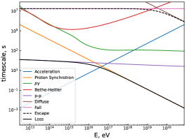
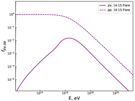
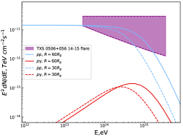
Figure 1: The panels, from left to right, show the various timescales, the efficiencies of $pp$ and $p\gamma$ interactions, and the neutrino spectrum in the MAD scenario. In panel (c), the observed neutrino spectrum of TXS 0506+056 during the 2014-2015 neutrino flare is also shown(IceCube Collaboration et al., 2018b). We adopt the parameter values of $M_{\rm BH}=3\times 10^{8}$, $\epsilon_{CR}=0.1$, $\epsilon=0.01$ and $\dot{m}=10$. In panel (a) and panel (b), the dissipation radius is set as $30R_{g}$, while in panel (c), two radius with $R=30R_{g}$ and $R=60R_{g}$ are assumed.

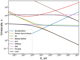
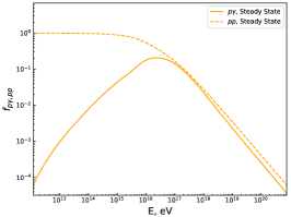
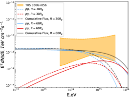
Figure 2: Same as Fig.1, but assuming $\dot{m}=0.1$ to explain the time-integrated neutrino emission of TXS 0506+056(IceCube Collaboration et al., 2022).

3 Neutrino emission from the accretion flow in the MAD and SANE scenarios

A magnetically arrested accretion disc (MAD, see Narayan et al. (2003a); Bisnovatyi-Kogan & Ruzmaikin (1974); Igumenshchev et al. (2003); Tchekhovskoy et al. (2014)) may be present in TXS 0506+056 since magnetohydrodynamical (MHD) simulations have shown that it can launch powerful jets (e.g. Tchekhovskoy et al. (2011)). In this situation, a large-scale poloidal magnetic field prevents gas from accreting continuously at a magnetospheric radius. Around the magnetospheric radius, the gas flow breaks up into a blob-like stream and moves inward by diffusing via magnetic interchanges through the magnetic field. We also consider the standard and normal evolution (SANE) regime of accretion, where the magnetic field that accumulates around the BH is relatively weak.

3.1 The MAD scenario

MADs dissipate their magnetic energies through plasma processes, such as magnetic reconnection (Ball et al., 2018; Ripperda et al., 2020), and nonthermal particles are efficiently accelerated by reconnection (Hoshino, 2012; Sironi & Spitkovsky, 2014; Werner et al., 2018) and/or turbulence (Lynn et al., 2014; Kimura et al., 2019).

In the MAD scenario, the proton number density in the accretion flow is $n_{\rm p,MAD}=\dot{M}/4\pi m_{p}RHV_{\rm R,MAD}$, where $V_{\rm R,MAD}=\epsilon V_{ff}$ is the radial velocity, $V_{\rm ff}=\sqrt{2GM_{\rm BH}/R}$ is free-fall velocity and $\epsilon\lesssim 0.01$ (Narayan et al., 2003b). Taking $H=R/2$, we have

$$n_{p,\rm{MAD}}\sim 7.3\times 10^{12}~{}\rm{cm}^{-3}$$ (11)

$$\left(\frac{\dot{m}}{10}\right)\left(\frac{0.01}{\epsilon}\right)\left(\frac{{M}_{\rm BH}}{3\times 10^{8}M_{\odot}}\right)^{1/2}\left(\frac{R}{30R_{g}}\right)^{-3/2}$$

Here we consider a dissipation site with a radius $R\sim 30-60R_{g}$ for the MAD scenario. For smaller $R$, the cooling of protons due to synchrotron emission would be too strong and the neutrino emission will be suppressed (as discussed later).

The magnetic field of MAD can be obtained by equating the magnetic energy density $B_{\rm MAD}^{2}/(8\pi)$ with the gravitational force per unit area of the radially accreting mass $GM_{\rm BH}m_{p}n_{\rm p,MAD}H/R^{2}$, which is given by

$$B_{\rm MAD}=\sqrt{\frac{2GM\dot{M}}{\epsilon V_{ff}R^{3}}}$$ (12)

$$\sim 6\times 10^{4}\,{\rm G}\left(\frac{M_{\rm BH}}{3\times 10^{8}M_{\odot}}\right)^{3/2}\left(\frac{\dot{m}}{10}\right)\left(\frac{0.01}{\epsilon}\right)\left(\frac{R}{30R_{g}}\right)^{-5/2}.$$

Then the acceleration timescale is given by

$$t_{\rm acc,MAD}\approx\frac{\eta r_{\rm L}}{c}$$ (13)

$$\simeq 55\,{\rm s}\left(\frac{E_{p}}{100\rm{PeV}}\right)\left(\frac{\eta}{300}\right)\left(\frac{B}{6\times 10^{4}~{}G}\right)^{-1}\,{\rm s},$$

The timescale of diffusion is $t_{\rm diff}\approx R^{2}/D_{\rm R}\sim 6.4\times 10^{9}rm{s}(R/30R_{g})^{2}(E_{p}/2\,{\rm PeV})^{-1}\,$s and the timescale of advection is $t_{\rm fall}\approx R/V_{\rm R}\simeq 1.7\times 10^{7}rm{s}(R/30R_{g})^{-1/2}(\epsilon/0.01)\,$s respectively. The $pp$ cooling timescale is

$$t_{pp,\rm{MAD}} \approx 1/n_{p}{\sigma}_{pp}\kappa_{pp}c$$ (14)

$$\sim 230s\left(\frac{\dot{m}}{10}\right)^{-1}\left(\frac{M}{3\times 10^{8}M_{\odot}}\right)^{1/2}\left(\frac{R}{30R_{g}}\right)^{-3/2}.$$

The proton synchrotron timescale is

$$t_{p,\rm{syn,MAD}} =\frac{6\pi m_{p}c}{\gamma_{p}\sigma_{T}B^{2}}\left(\frac{m_{p}}{m_{e}}\right)^{2}$$ (15)

$$\approx 12\,{\rm s}\left(\frac{E_{p}}{100\rm{PeV}}\right)^{-1}\left(\frac{B}{6\times 10^{4}~{}G}\right)^{-2}$$

In the $p\gamma$ process, the energy of high-energy protons and the energy of target photons is related by $E_{p}\varepsilon_{\gamma}\sim 0.15~{}\rm{GeV}^{2}$. Therefore, the energy of target photons is $\varepsilon_{\gamma}\sim 1.5~{}\rm{eV}$ for protons with $E_{p}\sim 100~{}\rm{PeV}$. The number density of target photons in accretion disk is $n_{\gamma}=L_{\rm disk}/4\pi R^{2}c\varepsilon_{0}\approx 3\times 10^{13}~{}\rm{cm}^{-3}(\textit{L}_{\rm disk}/4.7\times 10^{43}~{}erg~{}s^{-1})(\varepsilon_{\gamma}/1.5~{}eV)^{-1}(\textit{R}/30\textit{R}_{g})^{-2}$, where $L_{\rm disk}$ is the luminosity of the inner disk at 1.5 eV, which is obtained by Eq.6

Therefore, the timescale of photomeson process ($p\gamma$) can be estimated as

$$t_{p\gamma,\rm{MAD}}\approx 1/n_{\gamma}{\sigma}_{p\gamma}K_{p\gamma}c\simeq 10^{4}\,\rm{s}\left(\frac{n_{\gamma}}{3\times 10^{13}~{}\rm{cm}^{-3}}\right)^{-1},$$ (16)

The Bethe-Heitler timescale $t_{\rm B-H}$ is written in the same form of Eq.16 by replacing the cross section with $\hat{\sigma}_{\rm B-H}$, which is given by

$$t_{\rm B-H,\rm{MAD}}\approx 1/n_{\gamma}\hat{\sigma}_{\rm BH}c\simeq 1.4\times 10^{6}\,\rm{s}\left(\frac{n_{\gamma}}{3\times 10^{13}~{}\rm{cm}^{-3}}\right)^{-1}.$$ (17)

Comparing the estimated timescales in Eq. (16), Eq. (17), Eq. (14) and Eq. (15), we find that the proton synchrotron process dominates the cooling in the MAD scenario. By equating the acceleration timescale Eq.13 and the proton synchrotron timescale Eq.15, we can derive the maximum proton energy,

$$E_{p,\rm{max,MAD}}\approx 50\,\rm PeV\,\left(\frac{\dot{m}}{10}\right)^{-1/4}\left(\frac{\textit{R}}{30\textit{r}_{g}}\right)^{-5/8}$$ (18)

$$\left(\frac{M_{\rm BH}}{3\times 10^{8}M_{\odot}}\right)^{3/8}\left(\frac{\eta}{300}\right)^{-1/2}.$$

We show the various timescales in the panel (a) of Fig. 1 for $R=30~{}r_{g}$ and $R=60~{}r_{g}$ with super-Eddington accretion $\dot{m}=10$. We used strict expression of $p\gamma$ and Bethe-Heitler process when plotting the panels, given as

$$t^{-1}_{p\gamma,{\rm B-H}}=\frac{c}{2\gamma_{p}^{2}}\int_{\epsilon_{\text{th}}}^{\infty}\sigma(\bar{\epsilon})\kappa(\bar{\epsilon})\bar{\epsilon}\,d\bar{\epsilon}\int_{\bar{\epsilon}/2\gamma_{p}}^{\infty}\epsilon^{-2}\frac{dn}{d\epsilon}d\epsilon,$$ (19)

where $\gamma_{p}$ is Lorentz factors of protons, ${dn}/{d\epsilon}$ is the number density of seed photons, $\epsilon_{\text{th}}$ is the threshold energy of $p\gamma$ interaction, $\sigma$ is cross-section and $\kappa$ is inelasticity for $p\gamma$ and Bethe-Heitler process.

For protons energy below 100 TeV, $pp$ collision dominates the cooling process and $p\gamma$ is partly suppressed by the proton synchrotron emission in the energy range of 320 TeV to 32 PeV. From the above timescales, we can derive $pp$ and $p\gamma$ interaction efficiencies, which are shown in the panel (b) of Fig. 1. The efficiencies of $pp$ and $p\gamma$ process in the relevant proton energy range are roughly $f_{pp}\sim 0.9$ and $f_{p\gamma}\sim 0.01$ for typical parameter values, respectively. Hence, during the 2014-2015 period, the neutrinos from the core are predominantly produced by $pp$ collisions.

In panel (c) of Fig. 1, we show the neutrino spectrum in comparison with the observations by IceCube during the 2014-2015 neutrino flare period of TXS 0506+056. The solid line represents the neutrino spectrum for $R=60R_{g}$, whereas the dashed line represents the neutrino spectrum for $R=30R_{g}$. A smaller radius of the dissipation site leads to a larger magnetic field, thereby increasing the cooling of pions and protons and leading to a lower cutoff energy in the neutrino spectrum.

We also consider the steady-state neutrino emission of TXS 0506+056 in the MAD scenario, where a lower accretion rate is applicable. We consider a sub-Eddington accretion rate with $\dot{m}\sim 0.1$ for TXS 0506+056. The corresponding timescales, the $pp$ and $p\gamma$ efficiency, and the neutrino spectrum are shown in Fig. 2. We find that $pp$ process dominates the $p\gamma$ process and this scenario can explain the 10-year time-integrated neutrino emission observed by IceCube (IceCube Collaboration et al., 2022).

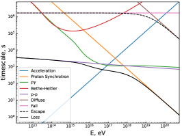
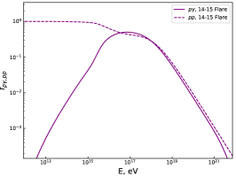
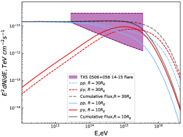
Figure 3: The panels, from left to right, show the various timescales, the efficiencies of $pp$ and $p\gamma$ interactions, and the neutrino spectrum in the SANE scenario. We adopt the parameters $M_{\rm BH}=3\times 10^{8}$, $\epsilon_{CR}=0.1$, $\alpha=0.3$, $\beta=10$ and $\dot{m}=10$. For panel (a) and panel (b), the dissipation radius is set as $30R_{g}$ and the plasma beta is set as $\beta=10$. In panel (c), the observed neutrino spectrum of TXS 0506+056 during the 2014-2015 neutrino flare is also shown and two radius with $R=10R_{g}$ and $R=30R_{g}$ are assumed.

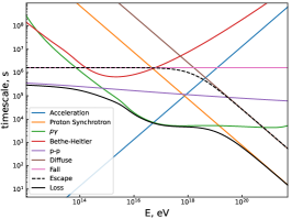
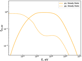
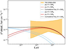
Figure 4: Same as Fig.3, but assuming $\dot{m}=0.1$ to explain the time-integrated neutrino emission of TXS 0506+056 (IceCube Collaboration et al., 2022).

3.2 The SANE scenario

In the SANE scenario, a lower magnetic field is expected in the accretion flow. We set the plasma $\beta$ as $\beta=10$ in the SANE scenario. The proton number density in the accretion flow is

$$n_{p,\rm{SANE}}\sim 2.7\times 10^{11}\rm{cm}^{-3}$$ (20)

$$\left(\frac{\dot{m}}{10}\right)\left(\frac{0.3}{\alpha}\right)\left(\frac{{M}_{\rm BH}}{3\times 10^{8}M_{\odot}}\right)^{1/2}\left(\frac{R}{30R_{g}}\right)^{-3/2},$$

where the radial velocity is $V_{\rm R,SANE}\approx\alpha V_{k}/2$ in the SANE scenario, $V_{k}=\sqrt{2GM/R}$ is Keplerian velocity and $\alpha\sim 0.3$ is the viscous parameter. Then the magnetic field is given by

$$B_{\rm SANE}=\sqrt{\frac{8\pi n_{\rm p,SANE}m_{p}C_{s}^{2}}{\beta}}\sim 2.5\times 10^{3}\rm{G}$$ (21)

$$\left(\frac{\dot{m}}{10}\right)^{1/2}\left(\frac{M_{\rm BH}}{3\times 10^{8}M_{\odot}}\right)^{3/4}\left(\frac{R}{30R_{g}}\right)^{-5/4}\left(\frac{\beta}{10}\right)^{-1/2}\left(\frac{\alpha}{0.3}\right)^{-1/2},$$

where $C_{s}\approx V_{k}/2$ is sound speed. The particle acceleration timescale is given by

$$t_{\rm acc,SANE}\simeq 1.3\times 10^{3}\,{\rm s}\left(\frac{E_{p}}{100\rm{PeV}}\right)\left(\frac{\eta}{300}\right)\left(\frac{B}{2.5\times 10^{3}~{}G}\right)^{-1}.$$ (22)

The timescale of diffusion is $t_{\rm diff}\approx R^{2}/D_{\rm R}\sim 2.6\times 10^{8}\rm{s}(R/30R_{g})^{2}(E_{p}/100~{}\rm{PeV})^{-1}$ and $t_{\rm fall}\approx R/V_{\rm R}\simeq 1.6\times 10^{6}rm{s}(R/30R_{g})^{-1/2}(\alpha/0.3)$ respectively. The cooling timescales of $pp$ collision and proton synchrotron emission are, respectively,

$$t_{pp,\rm{SANE}}\sim 6\times 10^{3}\,{\rm s}$$ (23)

$$\left(\frac{\dot{m}}{10}\right)^{-1}\left(\frac{\alpha}{0.3}\right)\left(\frac{{M}_{\rm BH}}{3\times 10^{8}M_{\odot}}\right)^{-1/2}\left(\frac{R}{30R_{g}}\right)^{3/2}$$

and

$$t_{p,\rm{syn,SANE}} \sim 7\times 10^{3}\,{\rm s}$$ (24)

$$\left(\frac{E_{p}}{100\rm{PeV}}\right)^{-1}\left(\frac{B}{2.5\times 10^{3}~{}G}\right)^{-2}.$$

For the photon field in the SANE scenario, the number density of target photons is estimated to be $n_{\gamma}=L_{\rm disk}/4\pi R^{2}c\varepsilon_{0}\approx 3\times 10^{13}~{}\rm{cm}^{-3}(\textit{L}_{\rm disk}/4.7\times 10^{43}~{}erg~{}s^{-1})(\varepsilon_{0}/1~{}eV)^{-1}(\textit{R}/30\textit{R}_{g})^{-2}$. Then the timescale of photomeson process ($p\gamma$) can be estimated as

$$t_{p\gamma,\rm{SANE}}\simeq 10^{4}\,{\rm s}\left(\frac{n_{\gamma}}{3\times 10^{13}~{}\rm{cm}^{-3}}\right)^{-1},$$ (25)

and the timescale of Bethe-Heitler is

$$t_{\rm B-H,SANE}\simeq 1.4\times 10^{6}\,{\rm s}\left(\frac{n_{\gamma}}{3\times 10^{13}~{}\rm{cm}^{-3}}\right)^{-1}..$$ (26)

From the above timescales, we find that in the SANE scenario, the $pp$ process is the dominant cooling mechanism for the highest energy protons under typical parameter values. By equating the acceleration timescale with the $pp$ cooling timescale, we obtain the maximum proton energy,

$$E_{p,\rm{max,SANE}}\approx 400\,{\rm PeV}$$ (27)

$$\left(\frac{\dot{m}}{10}\right)^{-1/2}\left(\frac{M_{\rm BH}}{3\times 10^{8}M_{\odot}}\right)^{1/4}\left(\frac{R}{30R_{g}}\right)^{1/4}\left(\frac{\beta}{10}\right)^{-1/2}$$

$$\left(\frac{\alpha}{0.3}\right)^{1/2}\left(\frac{\eta}{300}\right)^{-1}.$$

Different parameter values can alter the dominance of cooling effects. Once the $p\gamma$ process becomes the predominant mechanism for the proton cooling, the maximum energy is determined by equating the acceleration timescale with the $p\gamma$ timescale,

$$E_{p,\rm{max,SANE}}\approx 800\,{\rm PeV}$$ (28)

$$\left(\frac{\dot{m}}{10}\right)^{1/2}\left(\frac{M_{\rm BH}}{3\times 10^{8}M_{\odot}}\right)^{3/4}\left(\frac{R}{30R_{g}}\right)^{-5/4}\left(\frac{\beta}{10}\right)^{-1/2}$$

$$\left(\frac{\alpha}{0.3}\right)^{-1/2}\left(\frac{n_{\gamma}}{3\times 10^{13}~{}\rm{cm}^{-3}}\right)^{-1}\left(\frac{\eta}{300}\right)^{-1}.$$

The panel (a) of Fig.3 shows various timescales in the SANE scenario for an emission radius of $R=30R_{g}$. The low-energy segment is predominantly influenced by pp interactions, whereas the high-energy segment is partially dominated by both $p\gamma$ interactions and proton synchrotron emission. The efficiency for $pp$ and $p\gamma$ are shown in panel (b) of Fig.3, which gives $f_{\rm pp}\sim 1$ and $f_{p\gamma}\sim 0.6$ in the neutrino energy range where the respective cooling process is dominated. In panel (c) of Fig. 3, we show the neutrino spectrum in comparison with the observation data during the 2014-2015 neutrino flare period of TXS 0506+056. Owing to a reduced magnetic field in the SANE scenario, the size of the dissipation region could be considerably smaller without suffering from a strong cooling for protons. Therefore we consider two dissipation radii with $R=10R_{g}$ and $R=30R_{g}$. We find that $pp$ and $p\gamma$ processes contribute significantly to the neutrino flux at lower and higher energies, respectively.

Same as the MAD scenario, we also consider the steady-state neutrino emission of TXS 0506+056 assuming a low accretion rate $\dot{m}\sim 0.1$. The corresponding timescales, the $pp$ and $p\gamma$ efficiencies, and the neutrino spectrum are shown in Fig. 4. Due to a lower density in the accretion flow, the $pp$ efficiency becomes lower. As a result, the $p\gamma$ process is dominant in the neutrino production in the observed energy range by IceCube.

4 Summary and discussion

In this work, we study whether the neutrino emission from TXS 0506+056 could come from the accretion flow, instead of the usually discussed relativistic jet. We find that a super-Eddington accretion with $\dot{M}\sim 10\dot{M}_{\rm Edd}$ is needed to explain the neutrino outburst during 2014-2015. The accretion flow may also produce the long-term neutrino emission during the steady state, where the accretion drops to sub–Eddington rate. The accretion flow could be a MAD with highly magnetized plasma. Magnetic reconnections and/or plasma turbulence in the MAD may accelerate cosmic ray particles, which produce neutrinos via $pp$ and $p\gamma$ processes. Compared with the SANE accretion flow, the MAD has a higher magnetic field, which leads to stronger cooling of cosmic ray protons. As a result, a larger radius for the dissipation in the MAD scenario is needed to avoid this cooling effect. The size of the neutrino production site is still sufficiently compact so that the TeV-PeV gamma-rays accompanied the neutrinos are absorbed by the dense optical to X-ray photons in the AGN core region.

In a super-Eddington accretion flow, $pp$ interactions play a dominant role in producing neutrinos because of the high density of the accretion flow. This lead to a flat neutrino spectrum with a high-energy cutoff, which is different from the neutrino spectrum of neutrino emission produced in the $p\gamma$ process. This may explain the hard neutrino spectrum in TXS 0506+056 during 2014-2015, in contrast to the soft spectrum of neutrino emission of NGC 1068, which is thought to be produced by the $p\gamma$ process.

5 Acknowledgements

We would like to thank B. Theodore Zhang and Hoaning He for helpful discussions on the long-term neutrino flux from TXS 0506+056. This work is supported by the National Natural Science Foundation of China (grant Nos. 12333006 and 12121003).

Note added.— While we were finalizing this manuscript, we became aware of the work of Zathul et al. (2024) (arXiv:24.14598), which also propose that the neutrino emission from TXS 0506+056 could originate near its AGN core.

References

- Acciari et al. (2022) Acciari, V. A., Aniello, T., Ansoldi, S., et al. 2022, ApJ, 927, 197, doi: 10.3847/1538-4357/ac531d
- Ball et al. (2018) Ball, D., Özel, F., Psaltis, D., Chan, C.-K., & Sironi, L. 2018, ApJ, 853, 184, doi: 10.3847/1538-4357/aaa42f
- Banik et al. (2020) Banik, P., Bhadra, A., Pandey, M., & Majumdar, D. 2020, Phys. Rev. D, 101, 063024, doi: 10.1103/PhysRevD.101.063024
- Bauer et al. (2015) Bauer, F. E., Arévalo, P., Walton, D. J., et al. 2015, ApJ, 812, 116, doi: 10.1088/0004-637X/812/2/116
- Bisnovatyi-Kogan & Ruzmaikin (1974) Bisnovatyi-Kogan, G. S., & Ruzmaikin, A. A. 1974, Ap&SS, 28, 45, doi: 10.1007/BF00642237
- Cerruti et al. (2019) Cerruti, M., Zech, A., Boisson, C., et al. 2019, MNRAS, 483, L12, doi: 10.1093/mnrasl/sly210
- de Gouveia Dal Pino et al. (2010) de Gouveia Dal Pino, E. M., Piovezan, P. P., & Kadowaki, L. H. S. 2010, A&A, 518, A5, doi: 10.1051/0004-6361/200913462
- Gámez Rosas et al. (2022) Gámez Rosas, V., Isbell, J. W., Jaffe, W., et al. 2022, Nature, 602, 403, doi: 10.1038/s41586-021-04311-7
- Gangadhara & Lesch (1997) Gangadhara, R. T., & Lesch, H. 1997, A&A, 323, L45, doi: 10.48550/arXiv.astro-ph/9707182
- Gao et al. (2019) Gao, S., Fedynitch, A., Winter, W., & Pohl, M. 2019, Nature Astronomy, 3, 88, doi: 10.1038/s41550-018-0610-1
- Hoshino (2012) Hoshino, M. 2012, Phys. Rev. Lett., 108, 135003, doi: 10.1103/PhysRevLett.108.135003
- Hoshino (2013) —. 2013, ApJ, 773, 118, doi: 10.1088/0004-637X/773/2/118
- Huang et al. (2020) Huang, J., Luo, B., Du, P., et al. 2020, ApJ, 895, 114, doi: 10.3847/1538-4357/ab9019