Quantum Wave Simulation with Sources and Loss Functions
keywords:
Numerical modeling, Wave propagation, Tomography, Quantum computing, Quantum algorithms, Quantum simulationWe present a quantum algorithmic framework for simulating linear, anti-Hermitian (lossless) wave equations in heterogeneous, anisotropic, but time-independent media. This framework encompasses a broad class of wave equations, including the acoustic wave equation, Maxwell’s equations, and the elastic wave equation. Our formulation is compatible with standard numerical discretization schemes and allows for efficient implementation of source terms for diverse time- and space-dependent sources. Furthermore, we demonstrate that subspace energies can be extracted and wave fields compared through an -loss function, achieving optimal precision scaling with the number of samples taken. Additionally, we introduce techniques for incorporating boundary conditions and linear constraints that preserve the anti-Hermitian nature of the equations. Leveraging the Hamiltonian simulation algorithm, our framework achieves a quartic speed-up over classical solvers in 3D simulations, under conditions of sufficiently global measurements and compactly supported sources and initial conditions. We argue that this quartic speed-up is optimal for time domain solutions, as the Hamiltonian of the discretized wave equations has local couplings. In summary, our framework provides a versatile approach for simulating wave equations on quantum computers, offering substantial speed-ups over state-of-the-art classical methods.
1 Introduction
Wave-based inverse problems are prevalent in disciplines such as seismology [1, 2, 3, 4], medical imaging [5, 6, 7], non-destructive testing [8, 9, 10], and meta-material research [11, 12, 13, 14]. However, the advancement of these fields is fundamentally limited by the current state of computational resources. In particular, the resolution and uncertainty quantification within imaging problems remain heavily restricted by computational capacities [15, 16, 17, 18, 19, 20, 21].
Quantum Computers (QCs) offer promising runtime improvements for numerous computational problems [22, 23, 24, 25]. One of the most promising groups of quantum algorithms is Hamiltonian Simulation (HS) algorithms. HS provides a framework for simulating quantum systems, i.e., the evolution of the Schrödinger equation, with up to exponential runtime advantages over classical solvers [26, 27, 28, 29]. A quantum state represented by two-state quantum particles or qubits has a state space dimension of . Classical algorithms for simulating its evolution under a quantum Hamiltonian scale at least linearly with the state size and, hence, exponentially with the number of qubits . In contrast, under specific conditions utilizing HS algorithms, a Quantum Computer (QC) is capable of performing quantum simulations with logarithmic scaling, thereby achieving an exponential speed-up compared to all classical computers:
Theorem 1 (Optimal sparse Hamiltonian simulation, ad. [27] - Theorem 3).
A -sparse Hamiltonian H on qubits with matrix elements specified to bits of precision can be simulated for time-interval , error , and success probability at least with queries to an oracle that provides a description of and a factor additional quantum gates.
The apparent question is: Can HS algorithms be used to simulate classical wave equations with the same runtime advantages? A growing body of research has explored the potential of HS for classical wave propagation problems. These studies examine source-free wave equations in homogeneous media [30, 31] or wave equations in media with varying parameters [32, 33, 34]. Each of these studies is focusing on a specific numerical approach, predominantly employing Finite Difference (FD) methods. Additionally, recent research has investigated solutions to mass-spring models [35, 36] that yield exponential runtime advantages in certain settings, with particular types of source terms considered in [37], or wave simulation problems addressed through warped phase transformations [38, 39, 40].
In this work, we demonstrate that for loss-free wave equations, including the elastic, acoustic, and electromagnetic case, a natural quantum encoding can be employed (Section 2), which enables a direct measurement of the wave field energy. Furthermore, by introducing the quantum encoding in the continuous domain, we effectively decouple it from discretization requirements, thus rendering our framework compatible with any numerical method.
We proceed by introducing algorithms to measure -related norms and subspace energies for extracting information from the simulated wave field (Section 3). Additionally, we propose a method to map sources to initial conditions, allowing efficient initialization on the QC (Section 4). Our overall objective is to establish an end-to-end speedup encompassing source initialization, simulation, and final state measurement. Achieving this requires each component to function cohesively, thereby realizing an advantage over classical computation.
Our primary result demonstrates that for sources and initial conditions with compact support, and when the measured quantities of the final state have sufficiently global characteristics relative to the system size, the proposed algorithmic framework achieves a quartic speedup in the three-dimensional case compared to all classical wave equation solvers. We argue that this runtime-advantage is optimal for time domain solutions of wave equations because of local couplings (Section 5).
2 A Natural Quantum Encoding for Linear, Anisotropic, Heterogeneous but Lossless Wave Equations
We consider wave equations of the form
| (1) |
where the wave field is an element of a Hilbert space containing at least once-differentiable and square-integrable -dimensional vector fields and is the source term. For concreteness, we have chosen Dirichlet Boundary Conditions on the domain boundary , where is a diagonal projector which selects the elements of the wave field on which we impose homogeneous Dirichlet BCs.
The operator is defined as
| (2) |
where is any Hermitian (self-adjoint) and positive-definite operator, and is any anti-Hermitian (anti-self-adjoint) operator with respect to the inner product
| (3) |
where , denotes complex conjugation, and and are any two wave fields. The operator is therefore anti-Hermitian with respect to the inner product
| (4) |
where
| (5) |
As we will discuss shortly, the inner product in (4) gives rise to a notion of energy that can be estimated on a QC. The anti-Hermiticity of with respect to is formalized by showing that
| (6) |
using integration by parts and invoking the BCs [41, 34]. Quantum states are naturally normalized with respect to a norm induced by the “quantum inner product” depicted in (3). Therefore, mapping (1) to a Schrödinger equation amounts to transforming , such that is anti-Hermitian with respect to . Because is Hermitian and positive-definite, it has a unique square root , which is also Hermitian and positive-definite. Transforming (1) with and leads to
| (7) |
We ignore the source term here, as it can be incorporated into the initial conditions or handled separately, as we will show in Section 4. Clearly, because is anti-Hermitian with respect to , it follows that is also anti-Hermitian with respect to the same “quantum inner product”. Multiplying (7) by the imaginary unit , we obtain a Schrödinger equation in its usual form with the corresponding Hamiltonian
| (8) |
Finally, observe that
| (9) |
Therefore, if induces a norm related to the energy of the system, so does on the transformed states.
2.1 The Acoustic Wave Equation
For -dimensional acoustics, we have that , where is the scalar pressure field and is the velocity field. The respective operators are given by [42]
| (10) |
and
| (11) |
The inner product relates to the sound energy as
| (12) |
2.2 Maxwell’s Equations
For Maxwell’s equations in dimensions, the state vector is defined as , where represents the electric field and represents the magnetic field. The operator containing the material properties is given by [41, 43]
| (13) |
where is the dielectric permittivity tensor and is the magnetic permeability tensor. These tensors reduce to a single coefficient times the identity for isotropic materials. For the presented framework to be applicable, both must be positive definite and Hermitian, thereby specifying a generally anisotropic but transparent medium without any losses [44].
We can further identify the anti-Hermitian operator
| (14) |
where is the curl operator. Finally, the inner product induced norm, which is related to the electromagnetic energy, can be identified as
| (15) |
2.3 The Elastic Wave Equation
In the interest of clear notation, we consider the linear elastic wave equation in 3D. Here, the state vector is given by , where is the particle velocity field and denotes the six independent entries of the positive definite and symmetric stress tensor . The corresponding strain tensor can be represented as . This notation allows us to represent the constitutive relations in the Voigt notation [45] as
| (16) |
where is the compliance matrix; a positive definite and invertible matrix for regular elasticity (e.g., odd elasticity can not be covered with this formulation [46]). Note that has at most independent parameters [47]. We can now identify
| (17) |
To be specific, we further introduce the divergence operator that acts on the stress vector as
| (18) |
With these definitions, we can find
| (19) |
Note that appears symmetric, but it is not: integration by parts, which shifts the derivative in the inner product introduces a minus sign, implying that . The elastic energy is now computed as
| (20) |
To see that the second term is indeed the potential deformation energy, let be the elasticity tensor in the Voigt notation. Then it can be readily verified that .
2.4 Numerical Discretization and Boundary Conditions
Our framework is compatible with any discretization method, provided that the (anti-)Hermitian properties of the operators are preserved. We represent the numerical discretization of the wave field and operators to vectors and matrices as , , , and . The discretized equations of motion read
| (21) |
where and incorporate the BCs (Section C.3).
Preserving the symmetry properties of these operators when discretizing requires that is a Hermitian matrix and an anti-Hermitian matrix. In Appendix C we exemplify the symmetry-preserving discretization of the acoustic wave equation using finite differences with a staggered grid. We further show that this discretization naturally gives Neumann or Dirichlet BCs on a rectangular domain. Then, starting from the discretization from these particular BCs that respect the symmetries, we discuss in Appendix D how one can introduce a general class of BCs that can be mapped to linear constraints [48]. This includes homogeneous or inhomogeneous Dirichlet or Neumann BCs along non-rectangular domain boundaries.
Additionally, must be a diagonal or block-diagonal matrix, with block sizes that are independent of the overall system size; otherwise, becomes dense, and the initial quantum state will lack sparsity. For instance, certain finite element methods produce non-block-diagonal mass matrices. To avoid this issue, we recommend using spectral element methods with Gauss-Lobatto-Legendre integration, which results in diagonal mass matrices [1] or finite differences.
3 Estimating Subspace -norms and Energies
Reading the complete discrete wave field comes with exponential and, hence, prohibitive costs. Consequently, it is essential to perform computations with the simulated wave field directly on the QC, e.g., by evaluating loss functions. We show that it is possible to efficiently measure -norms of subspaces containing multiple superposed quantum states, and that this measurement achieves optimal precision scaling with the number of experiment evaluations:
Theorem 2 (Subspace -norm, Section A.2).
Let . Given a projector , which projects onto a subspace , where each and , and let there be a state preparation oracle that prepares the quantum state ; then, if either or , there exists a quantum algorithm that efficiently estimates the squared sum of on as
| (22) |
with probability at least within error , which makes calls to the oracle (along with its inverse and controlled versions).
We will now apply this result to compare two wave fields, such as a simulated and a target -transformed wave field and to measure subvolume energies (see Section 2). By setting , where is the simulated wave field and is a target or observed wave field which is only defined or known within subvolume , we can write
| (23) |
This corresponds to an estimate of the -distance between both fields on subspace . By setting we obtain
| (24) |
which estimates the energy of on . Theorem 2 can also be used to compute energies and -comparisons of a superposition of multiple wave fields, extending the work of [35] on measuring energies. These multi-state - and energy estimates are key components of the source implementation algorithm, which we will introduce in Section 4.
To compare the states in the standard basis, we utilize a weighted inner product which reverses the transformation with :
Corollary 3 (Weighted -norm).
Given Theorem 2, we can estimate a weighted -norm with calls to the oracle (along with its inverse and controlled versions), as
| (25) |
where is a weight vector consisting of all unique weights. The estimation is efficient if the number of unique weights satisfies , and if for every either or .
Applying this to the comparison between two wave fields we obtain
| (26) |
where is the number of unique weights in the diagonal matrix , i.e. unique material parameters, and is the subspace only containing grid points with material parameters . Here, we need to assume that is diagonal in , which holds true for the acoustic wave equation or the isotropic Maxwell’s equation.
Given an efficient quantum algorithm for a unitary basis transformation, comparisons can also be performed in bases other than the computational basis. This, for example, includes the spatial frequency domain, which can be efficiently accessed through the quantum Fourier transform.
4 Implementing Sources
Incorporating time-dependent sources into the HS of classical wave equations poses a significant challenge when aiming to maintain efficient runtime scaling. We consider source terms of the form
| (27) |
where represents the spatial distribution and the temporal function of the source. We address the case of point sources in space, i.e., , where is any vector.
Assuming that is a pulse function, whose support in time is compact and with a length either constant or inversely proportional to its the maximum frequency, we will show that we can classically map the source to sparse initial conditions with an implementation complexity of . This already covers many practically relevant source scenarios. We then extend our approach to a broader class of sources that lack compact support in time.
4.1 Single Pulse Source
Consider a single point-source defined by . Its implementation complexity is tied to the number of values that need to be initialized on the QC. We identify two optimal scenarios:
4.1.1 Fixed Source Duration
If the simulation domain grows while the source remains active over a fixed duration , the implementation complexity naturally stays . This is achieved by:
-
1.
Classically solving the forced wave equation over within a fixed volume around the source, sufficient to contain all emitted waves during this interval.
-
2.
Initializing the resulting sparse wave field on the QC.
Since the required initialization volume does not scale with , only a constant number of grid points needs to be initialized, ensuring complexity.
4.1.2 Increasing Grid Resolution
When refining the grid to simulate higher-frequency wave pulses, typically the source time function includes higher frequencies, resulting in a duration inversely proportional to the increased frequency bandwidth :
| (28) |
where is the support of the Fourier transform of . For example, increasing the grid resolution by a factor of 2 (i.e., halving the spatial grid spacing ) allows us to resolve higher spatial frequencies. If we scale the frequency bounds of as and with , then this results in at least a doubling of and thus halving . Consequently, the classically simulated volume decreases proportionally across all dimensions, and the number of initialized grid points remains constant, maintaining complexity.
4.2 Multiple Pulse Sources
We extend our analysis to sources composed of multiple contributions as defined in (27).
4.2.1 Synchronized Activation
If all sources are active over the same time interval, i.e., and for all , the previous approach applies directly. Each source can be classically simulated within its respective volume, and the resulting wave fields are initialized on the QC as a single initial condition. The runtime scaling remains provided that the number of sources does not scale with .
4.2.2 Asynchronous Activation
When activation times vary among different point sources, an additional step is required to synchronize them. Let for denote the initial conditions from classically simulating each source over their respective durations . The combined and energy-transformed initial state is given by
| (29) |
where
| (30) |
The initial quantum state then is
| (31) |
incorporating initial conditions at different global times. To synchronize these states to a common global time , we evolve the state using a time-dilating Hamiltonian :
| (32) |
where
| (33) |
This effectively time-dilates each component, aligning them to . Subsequently, the synchronized state is evolved under the multi-state wave equation Hamiltonian to the final simulation time :
| (34) |
Due to the linearity of the wave equation, the superposition of partial wave fields in corresponds to the solution of (21) at time . Consequently, we can estimate an -distance to a target field or subspace energies using Theorem 2. Since the addition operation is inherently non-unitary, it must be integrated within the measurement process. Furthermore, as the loss function is nonlinear, we cannot compute losses for individual sub-fields separately and then combine them classically to derive the joint loss; therefore, we have to rely on Theorem 2 to estimate the loss function.
This approach remains efficient under the conditions that (a) the number of point sources is independent of , and (b) each individual source meets the previously outlined constraints.
4.3 General Sources
Implementing an arbitrary source time function that lacks compact support in time is inefficient with the above approach, as it results in initial conditions lacking compact support in space, which are prohibitively expensive to compute classically and initialize on the QC. However, under certain regularity assumptions about the medium surrounding the source, we can exploit rotational symmetries in the wave fields during initialization. Specifically, initial conditions, which satisfy rotational covariance can be implemented efficiently:
Lemma 4 (Vector Field Initialization, Section B.4).
Let , where . Assume that is rotationally covariant around a point in the first dimensions and invariant in the remaining dimensions. Consider an isotropic radially symmetric grid centered at , discretized into points, where is the number of radial divisions. The grid points are specified by radial indices and angular indices . Define the quantum state
| (35) |
where is the component of at grid point , and ensures normalization. This state can be initialized with classical evaluations of and quantum gates, where the tilde hides polylogarithmic factors.
Examples for include the -dimensional acoustic pressure field (), the acoustic particle velocity field, the electric field, and the magnetic field (all ). The elastic case is not included, as there .
Assuming a non-vanishing volume of homogeneous and isotropic material up to radius around the point-source location we can use analytic Greens functions to map the source to symmetric initial conditions:
Theorem 5 (Source initialization, Appendix B).
Let be a compactly supported function, and let be a rotationally covariant Green’s function around in the first dimensions and invariant in the remaining dimensions; at least up to radius , which is constant and non-vanishing. Define the time convolution . Using an isotropic radially symmetric grid centered at with points, the discretized quantum state encoding of can be initialized with classical evaluations and quantum gates, where the tilde hides polylogarithmic factors.
As the homogeneous and isotropic volume around the source is assumed to be small this method employs windowing as detailed in Appendix B and necessitates a combination of wave fields in the read out process as discussed in Section 4.2.2. The presented approach also allows for contributions that are not point-sources, as long as their combined initial fields satisfy rotational covariance and if is contained in the homogeneous and isotropic volume. If is non-symmetric, it can in some cases be decomposed into symmetric parts, provided the number of parts does not scale with , thus preserving the algorithm’s overall scaling. For multiple general source contributions (27), a separate spherical grid is required for each source. Bounding the error introduced in the loss function estimation by this approach is left for future research.
5 Runtime Advantage
Given that the discretized Hamiltonian (8) is -sparse, i.e. it has at most nonzero values in each row and column, which is ensured when and are -sparse matrices, quantum simulation requires operations (Theorem 1). In principle this offers an exponential speed-up over classical solvers, which all scale at least with [49, 50, 51, 52, 53]. However, as we now show, the obtainable speed-up is usually only polynomial [35]. In wave-based problems, increasing grid points typically aims to (i) enlarge the physical domain or (ii) increase the simulated frequencies. For systems with local couplings, such as those resulting from discretizing the considered wave equations, enlarging the domain requires a longer simulation time for waves to reach the boundaries. Similarly, a finer discretization to simulate higher frequencies raises due to the reduced grid spacing. As per Theorem 1, the number of query calls to scales linearly with both and . Consequently, the quantum speed-up over classical algorithms becomes a polynomial factor dependent on the spatial dimension . Specifically, let represent the simulation time for the signal to reach the domain boundary in dimensions. For classical algorithms scaling linearly with , the overall runtime complexity is . In contrast, the HS algorithm has runtime , where the tilde hides logarithmic factors. Thus, we expect a quadratic speed-up in 1D, cubic in 2D, and quartic in 3D. In contrast, [35] demonstrate an exponential speed-up for oscillator models with purely non-local couplings, where the simulation time does not scale with the system size.
Additionally, the algorithm’s oracle imposes constraints: to preserve quantum speed-up, the information transferred to the QC must be of order . This limits the number of independent material parameters defining the propagation this order, necessitating functional or low-dimensional material representations.
6 Limitations
The limitations considered here are those that either impact the algorithmic runtime in terms of big- complexity, or which are fundamentally not implementable in this framework.
6.1 Loss function Globality in Space and Compactness in Time
We identify two limitations within the introduced loss function estimations:
(i) Estimating time-dependent loss functions (as described in, e.g., [54]): Currently, our algorithm estimates the loss at a single measurement time step. Computing time-dependent loss functions involves separate simulation experiments for each measurement time, with the overall loss metric computed across all steps using either Theorem 2 or classical post-processing. However, this approach becomes inefficient for long comparison/integration times, where the number of comparison time steps scales worse than . Non-destructive estimation of the loss function [55, 56] could provide a solution by preserving the state throughout the measurement operation, enabling iterative evolution and loss estimation of the wave field for multiple time points.
(ii) Globality of measurement quantities: A limitation of QC loss estimation via observable measurements is the requirement for sufficiently global measurement quantities. Suppose a state is measured in a subspace with only a small probability amplitude fraction compared to the entire quantum state. In that case, more samples are needed to estimate the norm accurately, as the expected value becomes vanishingly small. Ensuring the subspace size is large with respect to mitigates this issue.
6.2 Compactness of Source Terms
We identify three limitations:
(i) The number of sources in space must not scale worse than . For instance, it is inefficient to have a source everywhere on the surface of a 3D body.
(ii) Situations in which the number of initial conditions grows polynomially with must be avoided to prevent restricting the overall runtime. An example of this could be a continuously active source within a domain of increasing size and simulation time.
(iii) For a general source term a radial symmetric grid is required. This may be practically limiting as domains are often non-symmetric around the source location. Additionally, the introduced vector field initialization algorithm does not cover cases where the vector field dimension is larger than the spatial one.
6.3 Damping
A significant limitation of the presented framework is its inability to implement damping due to its non-unitary nature. However, damping in the context of HS has been recently studied, demonstrating that quantum speed-up can be preserved under certain conditions [57]. An alternative approach is to map a damped classical wave equation to an open quantum system. Simulating such systems on QCs is a recent research focus [58]. We believe that our work can eventually be combined with these approaches.
6.4 Time-Dependent Media
A final remark concerns time-dependent media, such as those in time-modulated meta-materials [e.g., 59, 60, 61]. In these cases, becomes time-dependent, implying that it no longer commutes with the time derivative. Consequently, a time-dependent symmetric problem is mapped to a time-dependent non-Hermitian Schrödinger equation, rendering the introduced framework inapplicable [62].
7 Code
We present an educational Git repository, where we implement all the presented methods and concepts for the acoustic wave equation and Maxwell’s equations. The numerical implementation is based on a staggered grid finite difference method as detailed in Appendix C. The repository can be found here.
8 Conclusions
In this work, we have demonstrated that we can efficiently simulate forced, linear, anti-Hermitian wave equations with arbitrary heterogeneous and anisotropic material properties within the HS framework. While the theoretical speed-up of this approach can be exponential, practical 3D applications are expected to see a quartic speed-up due to the scaling of the simulation time with the system size. This quartic speed-up is maintained throughout our algorithm if the state read-out is sufficiently global compared to the overall system size.
Our method is compatible with any numerical approach that respects the anti-Hermitian nature of the operator and results in a diagonal or block diagonal representation of the material properties. The introduced representation of the wave equations naturally leads to a quantum encoding that enables the measurement of energies in subspaces of the model with optimal precision scaling. Additionally, we have shown that the -distance of the final simulated wave field to a target or observed wave field can be measured with optimal precision scaling and that a broad class of source terms can be implemented efficiently.
Recent studies have indicated that HS could be feasible on noisy QCs, potentially preceding the advent of noise-free quantum hardware [63, 64]. Furthermore, new advances in quantum error correction hint that noise-free QCs might be realized soon [65]. These findings suggest that our proposed framework may have practical applications in the near future, thereby underscoring the importance of continued research in this field. Our future research will focus on oracle free and optimal encodings of the evolution Hamiltonian and the material transforms.
Acknowledgements.
We would like to thank Dr. Scott Keating for helpful discussions on the loss functions and Marion Dugué for insights on the source decompositions. Furthermore, we are thankful to Patrick Marty and Dr. Ines Ulrich for sharing insights on acoustic wave physics in the context of medical imaging and to Dr. Václav Hapla for initial brainstorming sessions.Grant Acknowledgment: C.B. was supported by the Swiss National Science Foundation through a Postdoc.Mobility Fellowship. Furthermore, we gratefully acknowledge the support provided by Google Quantum AI, which has significantly contributed to the advancement of this research.
Data statement: No data have been used for this research.
Code availability statement: All codes used in this work are available at
Author contribution statement: study conception: C. Bösch; sources: M. Schade and C. Bösch; loss functions and energy estimation: M. Schade and C. Bösch; acoustic FD implementation: G. Aloisi; general boundary conditions and constraints: G. Aloisi and C. Bösch; manuscript preparation: M. Schade, C. Bösch, G. Aloisi. All authors reviewed the results and approved the final version of the manuscript.
References
- [1] A. Fichtner, Full seismic waveform modelling and inversion. Springer Science & Business Media, 2010.
- [2] S. Cesca and F. Grigoli, “Full waveform seismological advances for microseismic monitoring,” Advances in Geophysics, vol. 56, pp. 169–228, 2015.
- [3] H. Igel, Computational seismology: a practical introduction. Oxford University Press, 2017.
- [4] S. J. Arrowsmith, D. T. Trugman, J. MacCarthy, K. J. Bergen, D. Lumley, and M. B. Magnani, “Big data seismology,” Reviews of Geophysics, vol. 60, no. 2, p. e2021RG000769, 2022.
- [5] R. G. Pratt, L. Huang, N. Duric, and P. Littrup, “Sound-speed and attenuation imaging of breast tissue using waveform tomography of transmission ultrasound data,” in Medical Imaging 2007: Physics of Medical Imaging, vol. 6510, pp. 1523–1534, SPIE, 2007.
- [6] H. Gemmeke and N. Ruiter, “3d ultrasound computer tomography for medical imaging,” Nuclear Instruments and Methods in Physics Research Section A: Accelerators, Spectrometers, Detectors and Associated Equipment, vol. 580, no. 2, pp. 1057–1065, 2007.
- [7] J. M. Sanches, A. F. Laine, and J. S. Suri, Ultrasound imaging. Springer, 2012.
- [8] S. O. Naffa, M. Goueygou, B. Piwakowski, and F. Buyle-Bodin, “Detection of chemical damage in concrete using ultrasound,” Ultrasonics, vol. 40, no. 1-8, pp. 247–251, 2002.
- [9] K. Kim and W. R. Wagner, “Non-invasive and non-destructive characterization of tissue engineered constructs using ultrasound imaging technologies: a review,” Annals of biomedical engineering, vol. 44, pp. 621–635, 2016.
- [10] A. Lopez, R. Bacelar, I. Pires, T. G. Santos, J. P. Sousa, and L. Quintino, “Non-destructive testing application of radiography and ultrasound for wire and arc additive manufacturing,” Additive Manufacturing, vol. 21, pp. 298–306, 2018.
- [11] M. P. Bendsoe and O. Sigmund, Topology optimization: theory, methods, and applications. Springer Science & Business Media, 2013.
- [12] R. E. Christiansen and O. Sigmund, “Inverse design in photonics by topology optimization: tutorial,” JOSA B, vol. 38, no. 2, pp. 496–509, 2021.
- [13] A. K. Sharma, M. Kosta, G. Shmuel, and O. Amir, “Gradient-based topology optimization of soft dielectrics as tunable phononic crystals,” Composite Structures, vol. 280, p. 114846, 2022.
- [14] G. Bordiga, E. Medina, S. Jafarzadeh, C. Boesch, R. P. Adams, V. Tournat, and K. Bertoldi, “Automated discovery of reprogrammable nonlinear dynamic metamaterials,” arXiv preprint arXiv:2403.08078, 2024.
- [15] Ö. Yilmaz, Seismic data analysis: Processing, inversion, and interpretation of seismic data. Society of exploration geophysicists, 2001.
- [16] A. Fichtner and J. Trampert, “Resolution analysis in full waveform inversion,” Geophysical Journal International, vol. 187, no. 3, pp. 1604–1624, 2011.
- [17] N. Rawlinson, A. Fichtner, M. Sambridge, and M. K. Young, “Seismic tomography and the assessment of uncertainty,” Advances in geophysics, vol. 55, pp. 1–76, 2014.
- [18] M. Betancourt, “A conceptual introduction to hamiltonian monte carlo,” arXiv preprint arXiv:1701.02434, 2017.
- [19] M. K. Sen and R. Biswas, “Transdimensional seismic inversion using the reversible jump hamiltonian monte carlo algorithm,” Geophysics, vol. 82, no. 3, pp. R119–R134, 2017.
- [20] A. Fichtner, A. Zunino, and L. Gebraad, “Hamiltonian monte carlo solution of tomographic inverse problems,” Geophysical Journal International, vol. 216, no. 2, pp. 1344–1363, 2019.
- [21] I. E. Ulrich, C. Boehm, A. Zunino, and A. Fichtner, “Analyzing resolution and model uncertainties for ultrasound computed tomography using hessian information,” in Medical Imaging 2022: Ultrasonic Imaging and Tomography, vol. 12038, pp. 48–60, SPIE, 2022.
- [22] M. A. Nielsen and I. L. Chuang, Quantum computation and quantum information. CUP, 2010.
- [23] A. Montanaro, “Quantum algorithms: An overview,” npj Quantum Information, vol. 2, no. 1, pp. 1–8, 2016.
- [24] M. Cerezo, A. Arrasmith, R. Babbush, S. C. Benjamin, S. Endo, K. Fujii, J. R. McClean, K. Mitarai, X. Yuan, L. Cincio, et al., “Variational quantum algorithms,” Nature Reviews Physics, vol. 3, no. 9, pp. 625–644, 2021.
- [25] J. M. Martyn, Z. M. Rossi, A. K. Tan, and I. L. Chuang, “Grand unification of quantum algorithms,” PRX Quantum, vol. 2, p. 040203, Dec 2021.
- [26] A. M. Childs and N. Wiebe, “Hamiltonian simulation using linear combinations of unitary operations,” arXiv preprint arXiv:1202.5822, 2012.
- [27] G. H. Low and I. L. Chuang, “Optimal hamiltonian simulation by quantum signal processing,” Physical Review Letters, vol. 118, no. 1, p. 010501, 2017.
- [28] G. H. Low and I. L. Chuang, “Hamiltonian simulation by qubitization,” Quantum, vol. 3, p. 163, 2019.
- [29] G. H. Low, Y. Su, Y. Tong, and M. C. Tran, “Complexity of implementing trotter steps,” PRX Quantum, vol. 4, no. 2, p. 020323, 2023.
- [30] P. C. Costa, S. Jordan, and A. Ostrander, “Quantum algorithm for simulating the wave equation,” Physical Review A, vol. 99, no. 1, p. 012323, 2019.
- [31] A. Suau, G. Staffelbach, and H. Calandra, “Practical quantum computing: Solving the wave equation using a quantum approach,” ACM Transactions on Quantum Computing, vol. 2, no. 1, pp. 1–35, 2021.
- [32] Y. Sato, R. Kondo, I. Hamamura, T. Onodera, and N. Yamamoto, “Hamiltonian simulation for time-evolving partial differential equation by scalable quantum circuits,” arXiv preprint arXiv:2402.18398, 2024.
- [33] Y. Sato, H. Tezuka, R. Kondo, and N. Yamamoto, “Quantum algorithm for partial differential equations of non-conservative systems with spatially varying parameters,” arXiv preprint arXiv:2407.05019, 2024.
- [34] M. Schade, C. Bösch, V. Hapla, and A. Fichtner, “A quantum computing concept for 1-D elastic wave simulation with exponential speedup,” Geophysical Journal International, vol. 238, pp. 321–333, 05 2024.
- [35] R. Babbush, D. W. Berry, R. Kothari, R. D. Somma, and N. Wiebe, “Exponential quantum speedup in simulating coupled classical oscillators,” Physical Review X, vol. 13, no. 4, p. 041041, 2023.
- [36] Y. Ito, Y. Tanaka, and K. Fujii, “How to map linear differential equations to schr”o dinger equations via carleman and koopman-von neumann embeddings for quantum algorithms,” arXiv preprint arXiv:2311.15628, 2023.
- [37] S. Danz, M. Berta, S. Schröder, P. Kienast, F. K. Wilhelm, and A. Ciani, “Calculating response functions of coupled oscillators using quantum phase estimation,” arXiv preprint arXiv:2405.08694, 2024.
- [38] S. Jin, N. Liu, and C. Ma, “Quantum simulation of maxwell’s equations via schröodingersation,” arXiv preprint arXiv:2308.08408, 2023.
- [39] S. Jin, N. Liu, and Y. Yu, “Quantum simulation of partial differential equations: Applications and detailed analysis,” Physical Review A, vol. 108, no. 3, p. 032603, 2023.
- [40] C. Ma, S. Jin, N. Liu, K. Wang, and L. Zhang, “Schr” odingerization based quantum circuits for maxwell’s equation with time-dependent source terms,” arXiv preprint arXiv:2411.10999, 2024.
- [41] S. G. Johnson, “Notes on the algebraic structure of wave equations,” Online at http://math. mit. edu/~ stevenj/18.369/wave-equations. pdf, 2007.
- [42] M. Kaltenbacher, Fundamental Equations of Acoustics, p. 12. Cham: Springer International Publishing, 2018.
- [43] D. J. Griffiths, Introduction to electrodynamics. Cambridge University Press, 2023.
- [44] S. G. Johnson and J. D. Joannopoulos, Photonic crystals: the road from theory to practice. Springer Science & Business Media, 2001.
- [45] W. Voigt, Lehrbuch der kristallphysik:(mit ausschluss der kristalloptik), vol. 34. BG Teubner, 1910.
- [46] C. Scheibner, A. Souslov, D. Banerjee, P. Surówka, W. T. Irvine, and V. Vitelli, “Odd elasticity,” Nature Physics, vol. 16, no. 4, pp. 475–480, 2020.
- [47] K. Aki and P. G. Richards, Quantitative Seismology, 2nd Ed. University Science Books, 2002.
- [48] J. Hoepffner, “Implementation of boundary conditions,” Software available at http://www. lmm. jussieu. fr/ hoepffner/boundarycondition. pdf, 2007.
- [49] L. Banjai and S. Sauter, “Rapid solution of the wave equation in unbounded domains,” SIAM Journal on Numerical Analysis, vol. 47, no. 1, pp. 227–249, 2009.
- [50] Z.-G. Qian and W. C. Chew, “Fast full-wave surface integral equation solver for multiscale structure modeling,” IEEE Transactions on Antennas and Propagation, vol. 57, no. 11, pp. 3594–3601, 2009.
- [51] J.-G. Wei, Z. Peng, and J.-F. Lee, “A fast direct matrix solver for surface integral equation methods for electromagnetic wave scattering from non-penetrable targets,” Radio Science, vol. 47, no. 05, pp. 1–9, 2012.
- [52] S. Omar and D. Jiao, “A linear complexity direct volume integral equation solver for full-wave 3-d circuit extraction in inhomogeneous materials,” IEEE Transactions on Microwave Theory and Techniques, vol. 63, no. 3, pp. 897–912, 2015.
- [53] F. Smith, S. Tsynkov, and E. Turkel, “Compact high order accurate schemes for the three dimensional wave equation,” Journal of Scientific Computing, vol. 81, pp. 1181–1209, 2019.
- [54] J. Virieux and S. Operto, “An overview of full-waveform inversion in exploration geophysics,” Geophysics, vol. 74, no. 6, pp. WCC1–WCC26, 2009.
- [55] A. W. Harrow and A. Y. Wei, “Adaptive quantum simulated annealing for bayesian inference and estimating partition functions,” in Proceedings of the Fourteenth Annual ACM-SIAM Symposium on Discrete Algorithms, pp. 193–212, SIAM, 2020.
- [56] P. Rall and B. Fuller, “Amplitude estimation from quantum signal processing,” Quantum, vol. 7, p. 937, 2023.
- [57] H. Krovi, “Quantum algorithms to simulate quadratic classical hamiltonians and optimal control,” arXiv preprint arXiv:2404.07303, 2024.
- [58] Z. Hu, R. Xia, and S. Kais, “A quantum algorithm for evolving open quantum dynamics on quantum computing devices,” Scientific reports, vol. 10, no. 1, p. 3301, 2020.
- [59] H. Nassar, H. Chen, A. Norris, and G. Huang, “Quantization of band tilting in modulated phononic crystals,” Physical Review B, vol. 97, no. 1, p. 014305, 2018.
- [60] H. Chen, L. Yao, H. Nassar, and G. Huang, “Mechanical quantum hall effect in time-modulated elastic materials,” Physical Review Applied, vol. 11, no. 4, p. 044029, 2019.
- [61] E. Galiffi, R. Tirole, S. Yin, H. Li, S. Vezzoli, P. A. Huidobro, M. G. Silveirinha, R. Sapienza, A. Alù, and J. B. Pendry, “Photonics of time-varying media,” Advanced Photonics, vol. 4, no. 1, pp. 014002–014002, 2022.
- [62] C. Bösch, A. Fichtner, and M. S. Garcia, “Differences between quantum and classical adiabatic evolution,” arXiv preprint arXiv:2309.08510, 2023.
- [63] Y. Kikuchi, C. Mc Keever, L. Coopmans, M. Lubasch, and M. Benedetti, “Realization of quantum signal processing on a noisy quantum computer,” npj Quantum Information, vol. 9, no. 1, p. 93, 2023.
- [64] L. Wright, C. M. Keever, J. T. First, R. Johnston, J. Tillay, S. Chaney, M. Rosenkranz, and M. Lubasch, “Noisy intermediate-scale quantum simulation of the one-dimensional wave equation,” arXiv preprint arXiv:2402.19247, 2024.
- [65] R. Acharya, L. Aghababaie-Beni, I. Aleiner, T. I. Andersen, M. Ansmann, F. Arute, K. Arya, A. Asfaw, N. Astrakhantsev, J. Atalaya, et al., “Quantum error correction below the surface code threshold,” arXiv preprint arXiv:2408.13687, 2024.
- [66] R. Iten, R. Colbeck, I. Kukuljan, J. Home, and M. Christandl, “Quantum circuits for isometries,” Physical Review A, vol. 93, no. 3, p. 032318, 2016.
- [67] Y. He, M.-X. Luo, E. Zhang, H.-K. Wang, and X.-F. Wang, “Decompositions of n-qubit toffoli gates with linear circuit complexity,” International Journal of Theoretical Physics, vol. 56, pp. 2350–2361, 2017.
- [68] B. Zindorf and S. Bose, “Efficient implementation of multi-controlled quantum gates,” arXiv preprint arXiv:2404.02279, 2024.
- [69] E. A. Martinez, T. Monz, D. Nigg, P. Schindler, and R. Blatt, “Compiling quantum algorithms for architectures with multi-qubit gates,” New Journal of Physics, vol. 18, no. 6, p. 063029, 2016.
- [70] N. Goel and J. Freericks, “Native multiqubit toffoli gates on ion trap quantum computers,” Quantum Science and Technology, vol. 6, no. 4, p. 044010, 2021.
- [71] Y. Kim, A. Morvan, L. B. Nguyen, R. K. Naik, C. Jünger, L. Chen, J. M. Kreikebaum, D. I. Santiago, and I. Siddiqi, “High-fidelity three-qubit i toffoli gate for fixed-frequency superconducting qubits,” Nature physics, vol. 18, no. 7, pp. 783–788, 2022.
- [72] E. Knill, G. Ortiz, and R. D. Somma, “Optimal quantum measurements of expectation values of observables,” Physical Review A, vol. 75, no. 1, p. 012328, 2007.
- [73] R. F. Graf, Modern dictionary of electronics. Elsevier, 1999.
- [74] N. Gleinig and T. Hoefler, “An efficient algorithm for sparse quantum state preparation,” in Proceedings: 58th Design Automation Conference, pp. 433–438, IEEG, 2021.
- [75] E. Malvetti, R. Iten, and R. Colbeck, “Quantum circuits for sparse isometries,” Quantum, vol. 5, p. 412, 2021.
- [76] T. M. de Veras, L. D. da Silva, and A. J. da Silva, “Double sparse quantum state preparation,” Quantum Information Processing, vol. 21, no. 6, p. 204, 2022.
- [77] X.-M. Zhang, T. Li, and X. Yuan, “Quantum state preparation with optimal circuit depth: Implementations and applications,” Physical Review Letters, vol. 129, no. 23, p. 230504, 2022.
- [78] R. Vale, T. M. D. Azevedo, I. C. Araújo, I. F. Araujo, and A. J. da Silva, “Circuit decomposition of multi-controlled special unitary single-qubit gates,” IEEE Transactions on Computer-Aided Design of Integrated Circuits and Systems, 2023.
- [79] J. Virieux, “Sh-wave propagation in heterogeneous media; velocity-stress finite-difference method,” Geophysics, vol. 49, pp. 1933–1942, 11 1984.
- [80] R. L. Higdon, “Absorbing boundary conditions for acoustic and elastic waves in stratified media,” Journal of Computational Physics, vol. 101, no. 2, pp. 386–418, 1992.
- [81] J.-P. Berenger, “Perfectly matched layer for the fdtd solution of wave-structure interaction problems,” IEEE Transactions on antennas and propagation, vol. 44, no. 1, pp. 110–117, 1996.
- [82] R. Clapp, “Reverse time migration with random boundaries: 79th annual international meeting, seg, expanded abstracts, 2809–2813,” Geophysics, vol. 47, 2009.
- [83] X. Shen and R. Clapp, “Random boundary condition for memory-efficient waveform inversion gradient computation: Geophysics, 80,” R351–R359, 2015.
Appendix A Estimating Loss Functions
Lemma 6 (Two-state subspace -norm, Section A.1).
Let . Given a projector , which projects onto a subspace , where each and , and let there be a state preparation oracle that prepares the quantum state ; then, if either or , there exists a quantum algorithm that efficiently estimates the -norm between and on as
| (36) |
with probability at least within error , which makes calls to the oracle (along with its inverse and controlled versions).
A.1 Proof of Lemma 6
Here we consider the problem of estimating the -norm between two vectors on a subspace defined through the projector , where each and . We will prove that the problem can be solved with probability at least within error by calls to a state preparation oracle (along with its inverse and controlled versions), which prepares a quantum state if either or .
The squared -norm on this subspace is defined as
| (37) |
By introducing , we can write equation (37) as an expected value estimation
| (38) |
where the Hermitian observable is given by
| (39) |
The observable can be recognized as a difference operator that estimates the -norm between and on the subspace up to normalization and can, in principle, be implemented on a QC with sub-optimal precision scaling [22].
To estimate with optimal precision scaling beyond the central limit, we will introduce an auxiliary qubit to double the state space dimension. In this augmented space we can find a unitary decomposable observable , whose expectation value with respect to the augmented state is equal to , such that
| (40) |
We first demonstrate that there exists a unitary initialization procedure for given an initialization oracle for and discuss the efficiency of its implementation. We then explicitly construct , which can be decomposed into commuting unitary observables independent of and . We conclude by analyzing the overall complexity of our algorithm.
To start, let us combine preparing and preparing into a single unitary, , that prepares as
| (41) |
where . We further define the unitary matrix constructed from and its complement subspace as
| (42) |
By adding one auxiliary qubit, which is left invariant during the application of , the target state can finally be obtained as
| (43) |
where
| (44) |
As is diagonal, can be recognized as a permutation matrix, which is decomposable into . Each can be implemented with one multi-controlled X-gate (MCX). As MCX gates can be synthesized with controlled-not (CNOT) gates with a circuit depth of using auxiliary qubits [66, 67, 68], the overall gate complexity when implementing is with a circuit depth of . Hence, if either or , the implementation of is guaranteed to be efficient.
As future QCs might allow for implementing hardware native MCX-gates, further reductions in gate complexity are possible [69, 70, 71]. Additionally, regular patterns in can be exploited to implement multiple at once. Even for large , this can allow for an efficient implementation of in some instances, e.g., for projections to the first half of the domain.
We now introduce the augmented observable
| (45) |
Using the definition of detailed in equation (43), it is easy to check that
| (46) |
The augmented observable is always - independent of the state dimension and the subspace - represented by the 4 Pauli matrices
| (47) |
where
| (48) |
and with coefficients , such that
| (49) |
Hence, we conclude that can be estimated as
| (50) |
As proven in [72], the measurement of the expected value of a quantum state with respect to an observable that is unitary using high-fidelity amplitude amplification techniques has optimal precision scaling with a query complexity of . As all Pauli observables are unitary and the number of Pauli observables that represent is independent of and , it follows that our algorithm has the same query complexity.
A.2 Proof of Theorem 2
Building on Lemma 6, we can estimate general -norms of arbitrary many sub-states. Consider a quantum state
| (51) |
with , where is the number of sub-states. We aim to estimate a squared -norm, , on a subspace defined by the projector , such that
| (52) |
It remains to generalise (see equation (42)) and (see equation (49)).
We extend by recognizing that it corresponds to the unitary matrix
| (53) |
which is then tensor-multiplied with a number of -gates depending on , such that
| (54) |
Similarly, the specific structure of lets us define the generalized observable as
| (55) |
where
| (56) |
In this context, equation (55) represents the half-domain measurement of through
| (57) |
and the dimension of each sub-state as , while equation (56) describes the summation of the sub-states.
The number of Pauli observables in equation (56) depends on , as . Therefore, the number of unitary observables that need to be estimated is . For verification, with , , and , we see that and , confirming that .
Appendix B General Source Initialization
By definition, an isotropic radiator is a point source, which radiates the same intensity of radiation in all directions [73]. Examples of isotropic radiators include acoustic pressure sources or some radial vector field sources. In this section, we first show that an isotropic radiator acting in a homogeneous and isotropic domain generates a wave field, which satisfies rotational covariance around the point source location (Section B.3). We then utilize that rotationally covariant scalar and vector fields can be efficiently initialized on QCs (Lemma 4). Finally, we show that this initialization is also efficient if the homogeneous and isotropic volume around the point source is limited to radius , as long as source activation time does not scale with the system size. This establishes a general implementation method for isotropic radiators, which does not impact the end-to-end runtime of the forward model, and which only demands material restrictions in a small volume around the source. The method extends beyond homogeneous materials and even beyond isotropic radiators as long as rotation covariance is satisfied.
B.1 Homogeneous and Isotropic Medium
For concreteness, here we choose the acoustic wave equation in . We consider a point source located at within a homogeneous and isotropic domain. This source is active for a finite duration and is characterized by a source-time function . The 3D acoustic free-space homogeneous Green’s function reads [3]
| (58) |
where denotes the Dirac delta function. Clearly, exhibits radial covariance, meaning that its scalar solution remains constant for any fixed radius .
Next, let us consider the particle velocity solution of the Green’s function in the same setting, where the particle velocity is denoted by . The relationship between the particle velocity and the pressure field in a source-free, homogeneous, and isotropic acoustic medium is given by
| (59) |
where is the density of the medium. Substituting the pressure Green’s function into the above equation, we obtain
| (60) |
where is the Heaviside step function. Taking the spatial gradient, we have
| (61) | ||||
| (62) |
where is the unit radial vector. Substituting back, the particle velocity becomes
| (63) |
Simplifying, the vectorial Green’s function for the particle velocity is
| (64) |
We see that the particle velocities also exhibit rotational covariance, with orientations radial to the point source at a fixed . Consequently, the resulting time convolutions , which describes the initial pressure field, and , which describes the initial particle velocity field, inherit the radial covariance and invariance properties, as established in Section B.3. As a result, we can initialize this wave field efficiently on a QC with Lemma 4. Note, that the particle velocity vectors have radial orientation and hence a single dimensional component of the vector contains all information needed for the construction of the full wave field. Hence, we obtain an initialization complexity of quantum gates in the general -dimensional case, which is independent of the vector dimension .
B.2 Homogeneous Isotropic Medium in a Volume of Radius
Finally, let us consider a setting, where the material around the point source is only homogeneous and isotropic up to a radius and where the source activation time is greater than the travel time of the wave in the homogeneous domain . Here, the wave leaves the homogeneous domain before the source terminates. Hence, the Green’s function solution to this system is usually no longer analytically derivable and it does not satisfy rotational covariance around the source location. In this context, the previously introduced source implementation method is no longer applicable in its simple form. However, as long as is not vanishing, we can extend the method to this setting, as we will now show.
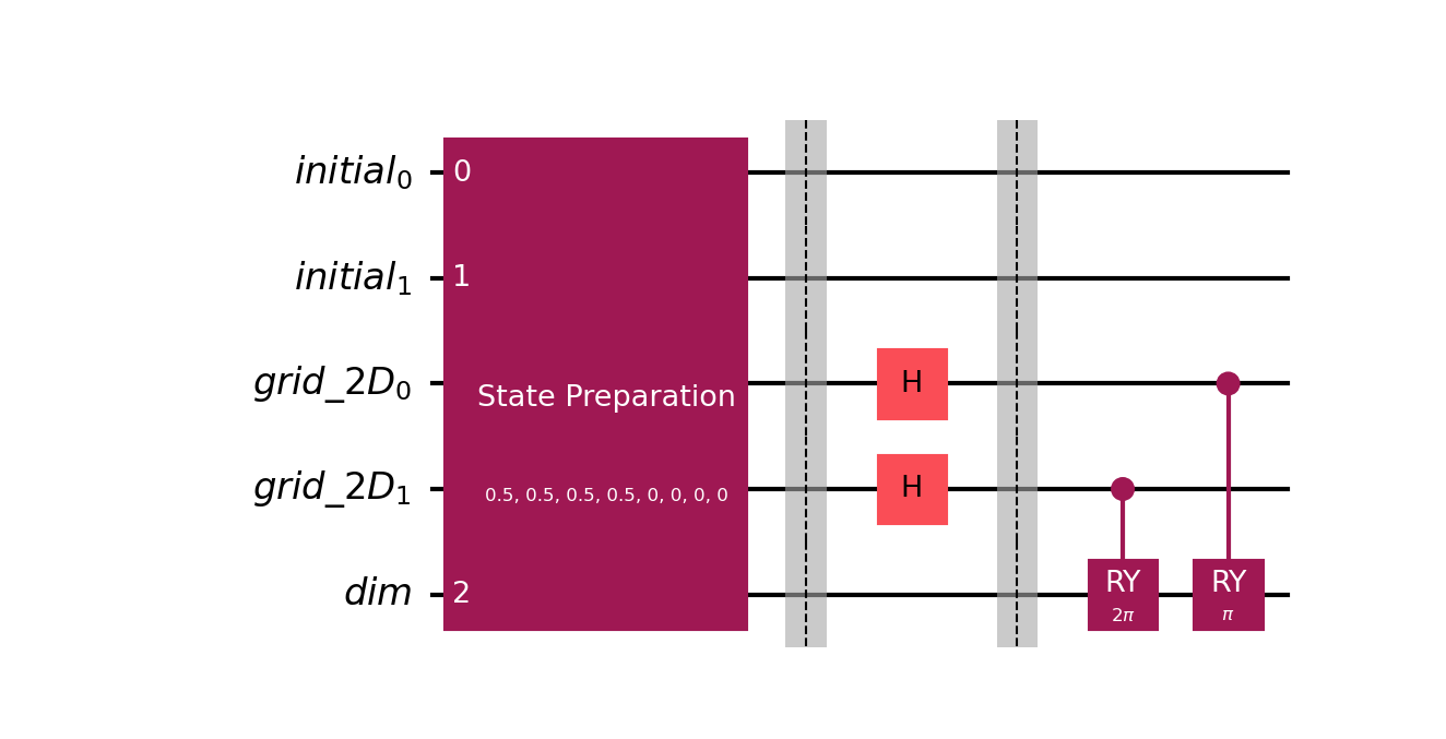
We will first discuss how the source can be decomposed, leading to multiple initial conditions. Then, we address the issue of evolving these initial conditions that start at different times, using a time-dilating Hamiltonian so that they all reach the same global time. Once all the initial conditions have reached the same time, they can be simulated in parallel under the same Hamiltonian with zero overhead toward the final time of simulation, . The entire workflow is depicted in Figure 1. Finally, Theorem 2 allows us to sum the individual wave fields to compare their superposition to a target state or to estimate subspace energies.
The point-source function can be split into windows by multiplication with time window functions , where is the time shift of the window. There exists multiple approaches of defining such that
| (65) |
is a sufficiently accurate approximation. Defining the window functions and time shifts in a way such that the initial condition in both and are smooth after multiplication is crucial for eliminating numerical dispersion effects in the subsequent HS. For the acoustic problem, this can be achieved with a symmetric double sigmoid function
| (66) |
where defines the steepness of the sigmoid functions. This function realizes overlapping windows that satisfy equation (65) with adaptable accuracy. In contrast to, e.g., box window functions (), sigmoid functions lead to smooth initial conditions. However, because the sigmoid functions do only converge to at the window boundary in the limit where , choosing a finite provides a trade-off between source approximation accuracy and smoothness of the sections. All source terms for (see equation (65)) can be recognized as individual sources that satisfy , meaning that for none of them, their wave leaves the homogeneous domain before it terminates.
We can now represent each in terms of initial conditions as
| (67) |
These initial conditions now individually satisfy rotational covariance around and can hence individually be implemented efficiently. The introduced method of Section 4.2 can now be used to synchronize them to the same global time and to estimate loss functions that superpose all wave fields, which is efficient if is independent of .
B.3 Covariance and Invariance Inheritance
Given the convolution defined by
| (68) |
we aim to show that inherits the rotational covariance and invariance properties of .
Rotational Covariance: Let , where acts on the first dimensions. Using the rotational covariance of and the linearity of convolution, we have
| (69) |
Thus, is rotationally covariant.
Invariance: For any , using the invariance of ,
| (70) |
Therefore, is invariant in the remaining dimensions. Combining both properties, we conclude that inherits the rotational covariance and invariance of .
B.4 Proof of Lemma 4
Our goal is to efficiently prepare the quantum state that encodes the vector field on an isotropic radially symmetric grid centered at .
Exploiting Rotational Covariance
Since is rotationally covariant around in the first dimensions and invariant in the remaining dimensions; that is, for any rotation that decomposes as , where and is the identity in , we have
| (71) |
Grid Construction
We discretize the space around into a grid as follows:
-
•
Radial Coordinates: The radial distance is discretized into divisions , where .
-
•
Angular Coordinates: Each angular coordinate is discretized into divisions, for .
-
•
Grid Points: Each grid point is specified by
(72) where is a unit vector determined by the angular indices .
-
•
Total Number of Points: (for .
Efficient State Preparation Strategy
We proceed with the following steps:
Step 1: Compute Reference Field Values
Select a reference direction, such as along the first coordinate axis, and compute for , where
| (73) |
and is the unit vector along the first coordinate axis. This requires classical evaluations of .
Step 2: Prepare Reference Quantum State
Step 3: Create Superposition Over Angular Indices
Apply Hadamard gates to the angular index qubits to create the equal superposition
| (75) |
Step 4: Apply Controlled Rotations
Our goal is to rotate the field components in to their correct orientations corresponding to each angular index .
This is achieved by applying a sequence of controlled rotations, where the rotation angles are determined by the angular indices , and the rotations are performed in the planes spanned by pairs of coordinate axes.
Specifically, we proceed as follows:
-
1.
Binary Representation of Angular Indices: Each angular coordinate is discretized into divisions and represented using qubits. For , the total number of angular qubits is .
-
2.
Rotation Decomposition: To rotate the initial vector to all possible directions , we decompose the rotation into a sequence of rotations. Specifically, we perform rotations in the -planes for :
(76) where is a rotation in the plane spanned by the and coordinates, parameterized by the angle determined by .
-
3.
Sequence of Controlled Rotations: For each plane , we apply controlled rotation gates , where indexes the bits in the binary representation of the angular coordinate . The rotation angles are defined as:
(77) so that the cumulative rotation angle , where is the bit of .
The controlled rotations are defined as:
(78) where is the qubit of the angular index corresponding to the rotation in the -plane. As the control qubits are in a state of equal superposition, all binary combinations of rotation angles are realized.
-
4.
Control and Target Qubits: The control qubits are the angular index qubits , and the target qubits are the field component qubits .
Gate Complexity
The total number of controlled rotation gates required is , since for each of the planes, we apply controlled rotations corresponding to the bits of the angular indices.
Since , the total number of controlled rotations is .
However, for a fixed spatial dimension the gate complexity of implementing these rotations [78] is dominated by the complexity of initializing , which requires quantum gates [74, 75, 76, 77].
Final State Preparation
After applying the sequence of controlled rotations, the state becomes
| (79) |
where we used the fact that due to the rotational covariance property. This is the desired state .
Practical Considerations
Applying requires implementing rotations with angles that decrease exponentially with the number of qubits used to represent the angular coordinates.
In practice, this poses challenges due to the finite precision of quantum gates.
Specifically, the minimal rotation angle scales inversely with the state size , resulting in a gate precision requirement that scales linearly with .
However, the precision requirement remains independent of .
This independence allows for the implementation of a larger total number of grid points without necessitating additional precision.
Numerical Implementation
We provide numerical implementations for the 2D and the 3D case in the supplements to the publication.
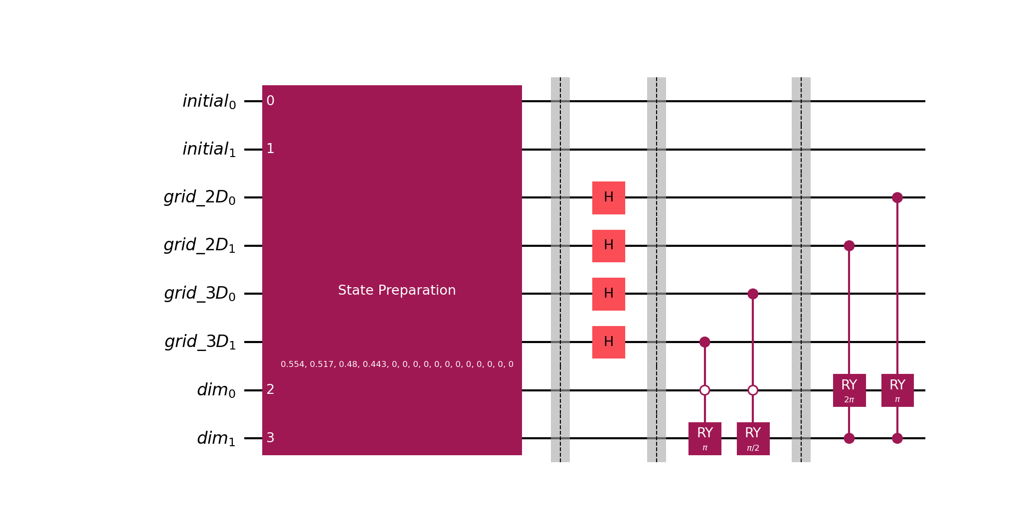
Figure 2 shows the quantum circuits for the 2D and 3D case that construct the radially symmetric vector field from a single ray.
Figure 3 shows the final output vector fields in 3D, where each vector element in the initialization ray points either in the -, -, or -direction.
Conclusion
By exploiting the rotational covariance of and the symmetry of the isotropic grid, we have shown that the quantum state can be initialized with classical evaluations of and quantum gates, where the tilde hides polylogarithmic factors.
This marks a polynomial improvement for a spatial dimension over the conventional initialization, which requires at least quantum gates if the number of auxiliary qubits used is kept constant [74, 75, 76, 77].
Appendix C Finite Difference Discretization for the Acoustic Wave equation
In this Appendix section, we discuss the discretization of the wave equation using the FD method on a uniform, rectangular, and staggered grid [79]. We show how to build a pair of discrete gradient and divergence operators to ensure that is anti-Hermitian (see Section 2). We also discuss the implementation of Dirichlet and Neumann BCs on arbitrary boundaries of the domain by employing the constraints reduction introduced in Appendix D.
Recall the acoustic wave equation in pressure-velocity formulation introduced in Section 2.1
The FD method aims to construct the mapping and by defining the discrete versions of the gradient and divergence operators that will be applied to the discretized pressure fields and respectively. The gradient and divergence operators are constructed independently of the BCs and follow from the definition of the FD operator used to approximate derivatives in space. Without loss of generality, we use the first-order accurate central-FD stencil to compute derivatives in the dimension
| (80) |
where is the canonical vector and is the grid step size in the direction. The gradient and divergence operators are then discretized accordingly, such that
| (81) | ||||
| (82) |
We now need to replace the continuous fields with their discretized counterparts by employing a staggered grid where the velocities are staggered in between pressure points. We introduce the set of numbers of grid points . Since the velocity is a vector field, we need to distinguish between velocities in different dimensions: we will use from now on to denote the velocity acting in the direction, such that where . Notice that this discretization imposes the discretized velocity field in the direction to have one less Degree of Freedom (DOF) in that direction. The pressure field is going to be discretized in DOF and the full velocity field in DOF.
C.1 2D Staggered Grid
We now demonstrate how the staggered grid is constructed in practice for the case, though the same procedure can be extended to the general -dimensional case.
In 2D, we have three fields: , , and , discretized on different grid points within a rectangular domain . Figure 4 provides a visual representation of the staggered grid used. Further details on its construction are described below.
We introduce the set of all grid points for the pressure field as follows
where , , , and . By staggering these points, we define the set of all grid points for the velocity field in the -direction and the -direction as
and
Notice that , , and .
The mappings from the linear indices of the discretized fields to the grid points are given by , , and . These mappings are constructed such that each index corresponds to one and only one grid point. For example, to map the pressure points, we introduce the Cartesian indices referring to the grid point at some position , and then linearize the Cartesian index using , so that . A similar linearization can be performed for the velocity mappings and .
We now have all the necessary components to explicitly formulate the semi-discretization of pressure and velocities
C.2 Discrete Gradient and Divergence Operators, and their Anti-Transpose Relationship
We construct the discretized gradient and divergence operators in 2D based on the first-order accurate central FD scheme introduced earlier. Generalization to FD schemes with higher orders of accuracy is straightforward since the symmetry of the FD operators is retained. Therefore, the results from this section remain unchanged when using higher-order schemes.
Let denote the row of the gradient operator . When taking the dot product of this row with the discretized pressure field , the FD approximation of a component of the gradient is computed for the semi-discrete equation concerning the discretized velocity field component . If refers to a discretized velocity component in the -direction (i.e., ), the -component of the gradient is computed; otherwise, the -component is computed.
This can be expressed by the following FD approximation
for all . Similarly, for the -component
for all .
For each equation (respectively, ), there will be only two non-zero coefficients in the row , specifically those associated with discretized pressure components matching (respectively, ). Here, represents the index of the discretized pressure component . These coefficients are (respectively, ).
With these observations, we can explicitly write each component of the gradient operator as follows
| (83) |
for all .
We can apply a similar procedure for the divergence operator using the FD approximation
resulting in
| (84) |
The anti-transpose property can be verified by showing that for all . This is easily checked by observing that the only difference in the definition of the operators and is the position of the mappings , (respectively, , ) in the conditions and (respectively, the conditions and ), which is the cause of sign flip of the components. This shows that the FD discretization using a uniform, rectangular, staggered grid produces a pair of gradient and divergence operators leading to an anti-Hermitian matrix .
C.3 Implementation of Boundary Conditions
The staggered grid described in the previous section naturally implements Neumann BCs, as the velocities in the direction perpendicular to the domain’s boundaries are assumed to be vanishing, i.e., for all , where is the normal vector at position on the boundary . A visual representation is shown in Figure 5(a), where the actual boundaries of the domain are depicted with a dashed line. To implement Dirichlet BCs, i.e., for all , constraints on pressure points with indices in the set must be added. Figure 5(b) provides a visual representation of these constraints. Using the method presented in Appendix D we can employ Dirichlet or Neumann BCs along arbitrary boundaries that align with the grid. An example for a rectangular grid with changing boundary conditions is displayed in Figure 5(c).
Since these added constraints result in a system where (see Appendix D), i.e., the unconstrained DOF do not appear in the constraint matrix , the modified matrices will be and , which are the original with some rows and columns removed corresponding to the newly constrained DOF.
Because the matrices and were Hermitian and anti-Hermitian by construction, respectively, the modified matrices and will remain Hermitian and anti-Hermitian, since deleting one row and column corresponding to the same index of a Hermitian (or anti-Hermitian) matrix results in a matrix that is still Hermitian (or anti-Hermitian).
Appendix D Generalizing Boundary Conditions to Linear Constraints
In Section C.3 we showed that in the acoustic case and for rectangular domains Neumann or Dirichlet BCs emerge naturally. In this section we introduce a general method to deal with BCs. The method operates directly on the discretized but general wave equation
| (85) |
where we aim to impose BCs as constraints. These constraints modify the wave equation and can introduce source terms. We assume that these constraints can be expressed in the following form:
| (86) |
where is the constraint matrix, is the number of constraints, represents the free (unconstrained) DOF, and represents the constrained DOF, which will be eliminated from the equations of motion. The vector is non-zero if the constraints are non-homogeneous. For example, in a 2D acoustic wave problem with FD discretization, homogeneous Dirichlet (Neumann) BCs along any boundary orthogonal to the or velocity components can be enforced by setting , and for all pressure (velocity) values on the boundary.
To incorporate the BCs (or constraints) into the wave equation, we follow the approach in [48]. We solve for the constrained DOF
| (87) |
Next, we rearrange the equations of motion to separate the free and constrained components
| (88) |
Rearranging the equations in this way preserves the Hermitian or anti-Hermitian nature of the matrices. Substituting (87) into the above equation and solving for the free DOF yields
| (89) |
where
| (90) |
and
| (91) |
For the constraints to be compatible with this approach, and must be Hermitian and anti-Hermitian, respectively. This condition is automatically satisfied when . In other cases, these conditions can be used to assess whether the constraints are implementable using a HS scheme, which relies on the Hermitian or anti-Hermitian properties of the matrices. The source term is given by
| (92) |
In general, this source cannot be implemented within our framework as the resulting wave field that needs to be initialized is neither radially symmetric nor populates a volume that is independent of . However, if is pulse-like and a point source in space, then the logic of Section 4.1 applies, giving rise to a quantum initialization that is independent on . Hence, certain boundary or displacement control problems can be implemented within the presented framework.
In summary, this scheme offers a practical approach to implementing BCs: First, discretize the equations, ensuring that the operators maintain the necessary Hermitian or anti-Hermitian properties, then introduce the BCs along the chosen boundaries as described.
Finally, absorbing boundaries or perfectly matched layers have played a crucial role in computational wave physics [80, 81, 1]. Due to their fundamentally non-energy conserving nature it is not straightforward to implement such BCs on a QC within the HS framework. However, they can approximately be implemented using random boundaries that diffuse the wavefield, thereby minimizing the energy that is back-scattered into the volume of interest [82, 83].