Wolfgang-Pauli-Strasse 27, 8093 Zürich, Switzerlandbbinstitutetext: Max Planck Institute for Gravitational Physics (AEI)
Am Mühlenberg 1, D-14476 Potsdam, Germany
Anomalous dimensions in the symmetric orbifold
Abstract
Recently, the anomalous conformal dimensions of the symmetric orbifold under the -cycle twisted sector deformation were calculated using the perturbed action of the supercharges. In particular, explicit and simple formulae for the dispersion relations of the torus magnons in the -cycle twisted sector were derived for large . In this paper we reproduce these results from a direct perturbed -point function calculation. In the process we also develop techniques (and a Mathematica code) that allows one to do these calculations for arbitrary quarter BPS states at finite .
1 Introduction
The symmetric orbifold of is dual to string theory on with one unit of NS-NS flux Gaberdiel:2018rqv ; Eberhardt:2018ouy ; Eberhardt:2019ywk . Recently, the perturbation that corresponds to switching on R-R flux in the dual AdS background was studied systematically in the symmetric orbifold Gaberdiel:2023lco , and the expected integrable structure of Babichenko:2009dk ; Hoare:2013lja ; Borsato:2013qpa ; Lloyd:2014bsa ; Frolov:2023pjw was recovered.
The analysis in Gaberdiel:2023lco was performed by determining the action of the supercharges on the various states to first order in perturbation theory, and then inferring the anomalous conformal dimensions from them. This approach generalised and refined previous calculations, see in particular Gava:2002xb ,111For other attempts to uncover the integrable structure underlying the symmetric orbifold see Lunin:2002fw ; Gomis:2002qi ; David:2008yk ; Pakman:2009zz ; Pakman:2009mi . and the structure that was found is very similar to the dynamical spin chain of SYM Beisert:2005tm , see Beisert:2010jr for a review. While this indirect method was very successful for SYM, it is quite delicate in the present context since in order for the integrable structure to emerge, it was not only necessary to consider the planar limit, but also a large charge limit . The latter is somewhat subtle since there are subleading terms (in ) in the action of the supercharges on the magnon states. These were systematically neglected in the analysis in Gaberdiel:2023lco , but they could, in principle, modify the answer for the anomalous dimensions.
In this paper we shall demonstrate that the approximation scheme of Gaberdiel:2023lco is indeed justified. More specifically, we shall determine the anomalous conformal dimensions by a direct second order perturbation theory calculation, and we find that this calculation reproduces nicely the predictions of Gaberdiel:2023lco . We should stress that while the second order perturbation theory does not make any approximations, it is much more involved, and can only be performed for relatively small values of .222Perturbative calculations of this kind had been studied before, see for example Keller:2019suk ; Benjamin:2021zkn ; Lima:2020boh ; Burrington:2012yq ; Guo:2022ifr ; Hughes:2023fot . On the other hand, the approach of Gaberdiel:2023lco defines a very efficient approximation scheme that allows one to read off the underlying integrable structure, something that would have been very difficult to extract from the full perturbation calculation.
1.1 The approach of Gaberdiel:2023lco
Let us be a bit more specific, and review the basic idea of the calculation in Gaberdiel:2023lco . We shall mainly concentrate on the -magnon states of the form
| (1.1) |
although we have also tested our results on other multi-magnon excitations. In the analysis of Gaberdiel:2023lco the action of a right-moving supercharge on this state was determined to first order in perturbation theory
| (1.2) |
where schematically accounts for the states that are not included in the first sum. One can check that the coefficients are suppressed as for large , and this motivated the limit prescription
| (1.3) |
Moreover, the then have a simple and suggestive form which can be formally continued to , thereby making contact with the integrability description of, for example, Lloyd:2014bsa . By considering the anti-commutator with the conjugate charge (for which a similar formula could be derived), the anomalous conformal dimension of (1.1) to second order in perturbation theory was then determined to be
| (1.4) |
1.2 The direct calculation
It is instructive to compare the above results to a direct determination of the anomalous dimension from calculating the perturbed -point function
| (1.5) |
where is the exactly marginal perturbing field,
| (1.6) |
and is the dimension BPS state (with spin up) in the 2-cycle twisted sector.
As indicated above, it is only the term proportional to that modifies the conformal dimension of , and it can be extracted as explained in Keller:2019suk . This calculation can be done directly using a suitable covering map, and we explain how this works in detail in Section 2 below. From that perspective one should then diagonalise the ‘anomalous dimension matrix’ , and one would expect that the anomalous conformal dimension of (1.4) should arise as the eigenvalue of the eigenstate that is a small deformation of .
As was explained in Benjamin:2021zkn , the two approaches are actually closely related to one another. In particular, the anomalous dimension matrix can be obtained from the different -point functions that appear in the analysis of eq. (1.2) via
| (1.7) |
where in each term the sum over accounts for all intermediate states of eq. (1.2), including the terms that are individually suppressed as . However, given that there are many intermediate states in the second sum of eq. (1.2), it is conceivable that these terms modify the result, and this is indeed what happens for the above matrix elements, see Section 2.2 below. In fact, by comparing the direct calculation of the left-hand-side with the different -point functions on the right-hand-side, we can explicitly determine which intermediate states contribute even at large , and we identify the additional intermediate states (beyond those that are accounted for by the first sum of eq. (1.2)) in Section 3.2. (The relevant states at large turn out to be certain -magnon states in the -cycle twisted sector.)
On the face of it, this seems to invalidate the approximation scheme of Section 1.1.333It would also indicate that the actual perturbation is not integrable since the additional intermediate states do not involve the same number of magnons. However, this conclusion is not correct: if we allow for arbitrary intermediate states in the anomalous dimension matrix as is automatic in the direct calculation of Section 2.1, it is inconsistent to restrict the external states to be only -magnon states of the form ! Thus if we want to determine the anomalous conformal dimensions from the direct mixing matrix, we need to diagonalise a much bigger matrix, that includes also -magnon states, etc. as external states. We find that, once this is done, the result reproduces nicely the prediction of eq. (1.4), see Section 2.3 below. This is the main result of our paper.
The relevant eigenstates of the anomalous mixing matrix involve in addition to the -magnon ‘head’ of the form (1.1), a ‘tail’ of - (and higher) magnon states. We also evaluate the supercharges on these eigenstates, and we find that, when restricted to the -magnon components, the action reduces to that of Gaberdiel:2023lco , see Section 3.4. Our analysis therefore demonstrates that the large approximation of Gaberdiel:2023lco captures the relevant algebraic structure (including the anomalous conformal dimensions) of the problem. At the same time, it is very efficient, and unlike the full calculation, see Section 2, one can extrapolate the answer to large .
We should mention that the full mixing matrix calculation is very complicated, and in order to do it efficiently, we had to write a Mathematica code that allows one to calculate the mixing matrix of in principle any two -BPS states to second order in perturbation theory. This code may also prove useful in other contexts, and we have therefore included it as an ancillary file to the arXiv submission.
The paper is organised as follows. In Section 2 we explain the ‘direct calculation’ of Section 1.2 in detail and show that the eigenvalues of the full problem reproduce the results of Gaberdiel:2023lco . The mixing matrix entries are reobtained in Section 3 from sums over intermediate states, i.e. as in eq. (1.7); in particular, this allows us to identify which intermediate states contribute to the mixing matrix for large . We also comment on the action of the supercharges on the eigenstates there, see Section 3.4. Our results are summarised in Section 4 and we give an outlook on future directions. There are two appendices to which some of the technical material has been relegated.
2 The four-point function calculation
In this section we outline the method of calculating the anomalous dimension using the direct method of Section 1.2.
2.1 The method of calculation
To order , the entries of the anomalous dimension matrix are given by Keller:2019suk
| (2.1) |
where is the perturbation in eq. (1.6), and our conventions are spelled out in Appendix A. This integral is regulated by cutting out disks around the insertions points. Using that the states we look at are -BPS, this can be further simplified by turning the surface integral into a contour integral:
| (2.2) |
Here, there are contours around the operator insertions at , and the operators in the correlator are BPS on the right,
| (2.3) |
The contour around can never contribute, by marginality of — this will be a consistency check on our calculations later.
2.1.1 The covering map
We will be interested in the anomalous dimension matrix, mixing states in the -twisted sector. The easiest way to calculate the relevant correlators is by using the covering map method Lunin:2000yv . For the situation at hand, the ramification profile is , and we only consider sphere coverings (since we are interested in the planar large limit). The covering map can then be described as
| (2.4) |
Here, we choose to parametrise the covering map by the position of the pole, , as was also done in Dei:2019iym for the special case . This has the advantage that the correlator will be single-valued in , making contour integration in principle straight-forward.
The covering map has the following properties. It is ramified at , with ramification indices , respectively. The ramification point unfixed by Möbius symmetry is
| (2.5) |
It maps onto the location of the perturbing field in the base space at
| (2.6) |
There are also quarter BPS states in the sector which can mix with our ‘in’ states. In order to calculate their matrix elements we thus also need the covering map with ramification profile ; this is given in Appendix B.2.
2.1.2 The anomalous dimension expressed through the covering map
Using the covering map, the calculation of the anomalous dimension in eq. (2.2) becomes444In the -contour integral, one needs to sum over all ‘diagrams’ contributing to the correlator, see Pakman:2009zz . Carrying out this sum corresponds to integrating over all of -space.
| (2.7) |
where the hat denotes the lift of the field to the covering surface. The contour of integration is around all of the , s.t. , which will be specified below.
The right-moving part of the correlator is the four-point function of (anti-)chiral primaries555We have made use of the freedom to shift the right-moving correlator by a constant to set the regular value at to zero for convenience.
| (2.8) |
where denotes the lift of the BPS state .
The main computational challenge, however, comes from the left-moving part of the correlator. Consider for example . The correlator can then be expressed as
| (2.9) |
The right-hand-side can now be computed using the Wick contractions of the free CFT on the covering surface. Once the contour integrals have been carried out, one is left with
| (2.10) |
where denotes the resulting correlator. We explain the details of one such sample calculation in Appendix B.1.
Let us close this section by describing the -contour integral in more detail. The relevant pre-images of are
| (2.11) |
These are the only pre-images of where the correlator can develop a singularity, as they correspond to . The superscript denotes the ‘channel’ of the intermediate fusion. The ‘’ stands for the case where the field which propagates in the middle is in the -twisted sector, the ‘’ stands for the case where it is in the -sector.
Additionally there are two pre-images of where the correlator can have a pole (corresponding to the diagrams where the twist-2 fields contract, ). They are
| (2.12) |
As mentioned before, however, there should not be any contribution from these ‘self-contractions’ of since the perturbation is exactly marginal. Confirming that this is indeed the case provides a non-trivial consistency check on our calculations.
2.2 Two-magnon external states
Armed with this formalism, one can then calculate for example the mixing of all the prototypical states, i.e. the anomalous dimension submatrix on the space
| (2.13) |
where the subscript refers to the fact that we are looking at 2-magnon excitations.
If we diagonalise this matrix, the mixing between different states is small and the eigenvalues are close to the diagonal elements. One observes that these do not approach the predicted spectrum eq. (1.4) for ; an essential difference is that the anomalous dimension for does not approach . In Fig. 1, the diagonal elements for are shown.
As explained above, the reason for this mismatch is that, if we include arbitrary intermediate states (as is automatic in this -point function calculation), we also need to consider the mixing matrix between arbitrary external states.
2.3 The full anomalous dimension matrix
In view of the above, we therefore have to consider arbitrary matrix elements, i.e. we cannot just evaluate the mixing matrix on the space from above. Instead we need to evaluate the mixing matrix on the space
| (2.14) |
where contains the states with magnon excitations. Additionally, there are states in the -twisted sector which can mix with as well, see Appendix B.2. Given that the perturbation preserves several charges, see Appendix A.1, only certain families of states can mix with the states in eq. (2.13), and we include in only those states for which this is possible. For example, the relevant four-magnon excitations on top of the BPS vacuum are
| (2.15) |
Because there is more freedom in how the are distributed over the component fields, one sees that the dimension of scales as , while , making the problem less tractable for large .666The dimension of scales as . However, at any finite , only the spaces up to and including are non-trivial. So while it is in principle possible to find the full mixing matrix, it quickly becomes unwieldy.
Calculating the anomalous dimension matrix when including these new states proceeds along the same lines as for the example in Appendix B.1. The details are more complicated, however: since there are also fermionic descendants, one needs additional types of contractions with many special cases, as the interaction with the spin-fields makes the fermionic correlators trickier than the bosonic ones. The full calculation thus quickly becomes overwhelming when written down by hand, and we have automated the process in Mathematica, allowing us to calculate any correlator of arbitrary external states. We have included the relevant Mathematica notebook as an ancillary file to the arXiv submission.
Since we are interested in relating our results to those of Gaberdiel:2023lco we will concentrate in the following on the eigenvalues associated to the two-magnon states . We select these by concentrating on the eigenstate of the full problem with maximal overlap , and we associate its eigenvalue to . We have carried out this calculation (including all external states) for small and extracted the spectrum this way. The states turn out to be low-lying in the spectrum. Furthermore, we find that one can obtain a good approximation to the eigenvalues by firstly restricting the mixing within the -twisted sector, and secondly by only including states with two or four magnon excitations, i.e. by projecting onto the space . This is sensible, as the mixing between and is suppressed by .
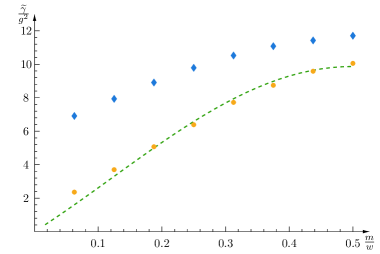
Using this approximation we can carry out the calculation for reasonably large , although much smaller than in Gaberdiel:2023lco . In Fig. 1, the result for is shown. One can see that at this intermediate value for , the spectrum is already very well described by the integrability dispersion relation in eq. (1.4). Explicitly, we find
| (2.16) |
where is some overall factor which can be absorbed by a rescaling of .
Let us stress how much more computationally expensive the full calculation is (relative to the approximation of Gaberdiel:2023lco ): to obtain the 8 points in Fig. 1, roughly 1500 states need to be taken into account. Each entry in the anomalous dimension matrix is computed by taking multiple analytic777In the computation, rational functions with large integer coefficients appear. Numerical computation becomes extremely unreliable, therefore the residues need to be taken analytically. residues, resulting in a large computational effort just to find the result for .
3 The three-point function calculation
In this section we explain how the calculation of the anomalous dimension matrix using four-point functions can be reproduced from three-point functions as in eq. (1.7). The reason to carry out this programme is three-fold. First of all, it allows us to determine which intermediate states effectively (i.e. in the large limit) contribute to the mixing matrix, see Section 3.2, and this then also informs what external states one should consider, see the discussion in Section 2.3 above. Secondly, it provides a highly non-trivial consistency check on the different calculations, see in particular Section 3.3. Thirdly, this algebraic calculation is directly comparable to Gaberdiel:2023lco , and we can gain a more microscopic understanding of why the analysis in Section 1.1 gives the correct result, see Section 3.4.
3.1 The method of calculation
As mentioned before, the anomalous dimension matrix on quarter BPS states can be decomposed into three-point functions where the supercharges act on the states Gava:2002xb ; Benjamin:2021zkn
| (3.1) |
and we specify below which states appear. The transitions in the expression above are a short-hand for the regulated three-point functions, appearing at first order in perturbation theory. For example,
| (3.2) |
where . Similarly,
| (3.3) |
We note that these correlators do not need to be integrated, and each of them can be calculated as explained in Gaberdiel:2023lco . In particular, we can lift the correlator to the covering surface where the fields are free and the calculation reduces to Wick contractions;888For the fermions, the spin field complicates things slightly. the relevant covering maps are
| (3.4) |
for transitions into the and -twisted sector, respectively.
The main difficulty of this method of calculation comes from the enumeration of the possible states and the calculation of a large number of correlation functions. We have automated this process with Mathematica.
3.2 Intermediate states
Let us explain how to identify the relevant intermediate states with the example of , where is one of the reference -magnon states in (1.1). We start by noting that must again be a -BPS state Keller:2019suk ; Benjamin:2021zkn . In addition, its dimension must be the same as that of , and we have the restrictions that come from the fact that the perturbation preserves various charges, see Appendix A.1 for more details. Given that the operator has right-moving R-charge and dimension , it maps into the -twisted sector.999 cannot map into the -twisted sector due to our choice of considering states whose right-moving part is the top BPS state in the -cycle twisted sector. Note that there is a ‘multi-trace’ BPS state with the correct charges in the -twisted sector, namely the state . However, transitions to this state are suppressed, and hence do not contribute in the planar (large ) limit. Furthermore, it is positively charged under the diagonal residual which rotates the bosons and is preserved by the perturbation (see Appendix A.1). This means that under we need to look at transitions to the states of the schematic form
| (3.5) |
where we have listed all the states with four or less magnon excitations. Only the first line describes the states considered in the original description of Gaberdiel:2023lco , but in general, transitions to all of these states are non-zero.
In addition to including these higher magnon states, one also needs to take into account that cannot only map into the -twisted sector, but also into the -twisted sector. This follows because we work with the top BPS state on the right, and in the -twisted sector there is a BPS state with charge , allowing the transition. However, the corresponding right-moving three-point function is actually suppressed with respect to the other transitions, see Appendix B.3.
3.3 Consistency checks
Once we take all possible intermediate states into account, we find that the three-point function calculation reproduces indeed exactly the four-point function calculation, as predicted by eq. (1.7). This is a highly non-trivial consistency check on both calculations.
We have carried out further consistency checks coming from the conservation of the algebra. For example we have confirmed that ; this is not trivially satisfied, but instead requires all possible intermediate states, once one includes some transitions beyond the -magnon sector. Another important identity is , which is also nontrivially satisfied and (indirectly) relates transitions to the -twisted sector to those to the -twisted sector. Finally, we have checked that , which requires the inclusion of transitions to multi-trace states.
3.4 Algebraic structure of the eigenstates
Given that the calculation of Gaberdiel:2023lco reproduces the correct anomalous conformal dimensions, one may expect that it also captures correctly the action of the supercharges, and this indeed turns out to be the case. In order to explain this, let us denote by the eigenstate associated to the two-magnon state , i.e. the eigenstate that has the largest overlap with . First, we find experimentally that each is annihilated by as well as ,101010To see this, one needs to take the mixing with the -twisted sector into account, which does not affect the spectrum. This additional complication is absent if one instead works with bosonic descendants of the bottom BPS state on the left, where one sees this property already when only looking at mixing in the -twisted sector. i.e. it sits in a short representation with respect to the superalgebra. As a consequence, the anomalous dimension of is simply given by
| (3.6) |
This is the basic algebraic structure also found in Gaberdiel:2023lco when applying the analysis to the states . Together with the matching of the anomalous dimensions shown in Fig. 1, this suggests that the full calculation is quantitatively controlled by the analysis of Gaberdiel:2023lco .
To find more evidence for this statement we explicitly study the action of on the eigenstate and compare it to the calculation in Gaberdiel:2023lco . Let us write the (normalised) eigenstate as
| (3.7) |
where is some numerical factor, and the ‘tail’ contains the other two-magnon states (with small coefficients), as well as higher magnon corrections. The operator maps this state into a linear combination of the form
| (3.8) |
The dominant transitions are to the states with and , for which the individual mode number of each magnon is approximately conserved.
Let us compare this to the calculation of Gaberdiel:2023lco , where at finite we only considered transitions from the schematic states of the form to those of the form . We can diagonalise the anomalous dimension matrix on this subspace, and obtain the naive ‘eigenstates’ which now only contain two-magnon states,
| (3.9) |
In this approach, the action of takes the form
| (3.10) |
where are the finite expressions from Gaberdiel:2023lco , and there is obviously no tail of multi-magnon states. We can now compare the coefficients to , and we find that there is very good quantitative agreement, already at small
| (3.11) |
More specifically, for and , the results are collected in Tab. 1.
| 1 | 0.32 | 0.31 |
|---|---|---|
| 2 | -0.04 | 0.01 |
| 3 | -0.01 | 0.00 |
| 4 | 0.01 | -0.01 |
| 5 | 0.07 | -0.02 |
| 6 | -0.77 | -0.76 |
Together with the fact that, see Fig. 1,
| (3.12) |
where is some -independent constant of proportionality (which can be absorbed in a rescaling of the coupling), and using the expression for the anomalous dimension as the norm of squared, see eqs. (3.6) and (3.11), one finds
| (3.13) |
Thus it follows that the complicated ‘tail’ only renormalises the ‘head’ of the state. This is the more microscopic reason why the limit of Section 1.1, see Gaberdiel:2023lco , captures the full analysis: it keeps track of the heads of the eigenstates from which one can read off the action of the supercharges, as well as the anomalous conformal dimensions. One would therefore expect that the corrections can be absorbed into a redefinition of the supercharges (and possibly also the magnon operators), so that they satisfy, in the large limit, the same relations as in (Gaberdiel:2023lco, , eqs. (5.24)). In particular, this would then make the integrable structure of the problem manifest.
4 Conclusions
In this paper we have studied in detail the perturbation in the symmetric product orbifold that is dual to turning on R-R flux in the background. We have mainly focused on one two-magnon reference state, see eq. (1.1), for which we have carried out the full calculation of the anomalous mixing matrix in the planar limit for twisted sectors up to , see Fig. 1. From this we have then extracted the dispersion relation for eigenstates associated to the two-magnon states, and we have shown that the spectrum reproduces (for large ) the one predicted in Gaberdiel:2023lco . Our analysis is therefore an independent consistency check of the results of Gaberdiel:2023lco , and in particular, justifies the large limit that was taken there. It also suggests that the limit of Gaberdiel:2023lco is naturally embedded in the full calculation, see the discussion in Section 3.4, and it would be interesting to explore this more systematically.
We have carried out the calculation of the anomalous dimensions in two ways, once by contour-integrating a four-point correlator, see Section 2, and once by summing over all possible three-point functions (OPE expansion), see Section 3. These calculations agree perfectly. Both methods can be applied to calculate the anomalous dimensions of any quarter BPS states in the planar limit of the orbifold, and may therefore also be useful in other contexts. (The relevant Mathematica notebooks are included as ancillary files in the arXiv submission.)
Acknowledgements
This paper is partially based on the Master thesis of one of us (F.L.). We thank Rajesh Gopakumar for initial collaboration and comments on a draft version of this paper, and Frank Coronado, Artyom Lisitsyn, Kiarash Naderi, and Vit Sriprachyakul for useful conversations. The work of BN is supported through a personal grant of MRG from the Swiss National Science Foundation. The work of the group at ETH is also supported in part by the Simons Foundation grant 994306 (Simons Collaboration on Confinement and QCD Strings), as well the NCCR SwissMAP that is also funded by the Swiss National Science Foundation.
Appendix A Conventions
We denote the left-moving four bosons and four fermions of the by , and , respectively. They satisfy the OPE relations
| (A.1) |
Right-movers are always denoted by a tilde. The (left-moving) generators are built out of these fields as
| (A.2) |
and
| (A.3) |
These fields generate the superconformal algebra, whose modes satisfy
| (A.4) |
as well as
| (A.5) |
and
| (A.6) |
The other (anti-)commutators vanish.
A.1 Conserved charges
The perturbation field is
| (A.7) |
where is the BPS state in the 2-cycle twisted sector (with spin up). This perturbation preserves the following charges:
-
•
The number of barred magnons. The bar charge acts as
(A.8) where stands for any free boson or fermion. This charge is conserved because all of the supercharges are neutral under ,
(A.9) -
•
The R-charge, i.e. the eigenvalue of , under which the fermions are charged
(A.10) -
•
There is a diagonal residual charge acting on the free bosons (and leaving the fermions invariant), which is also preserved by the perturbation. The residual left-moving charge is
(A.11) Then, the diagonal action, i.e. the simultaneous action on left- and right-movers, commutes with the perturbation
(A.12) In practice, since we look at quarter BPS states, this means that is preserved in the four-point function calculation. When calculating the anomalous dimension via three-point functions, we note that is positively charged under this symmetry, while is negatively charged. This restricts the possible intermediate states.
Appendix B Some calculational details
In this section we give some more details regarding the actual computation of the four- and three-point functions.
B.1 A -magnon matrix element
Here we show the basic method of the four-point calculation using covering maps. Let us consider the matrix element , where as before, see eq. (1.1)
| (B.1) |
are the normalised archetypal states. As discussed in Section 2.1.2, these matrix elements can be calculated on the covering surface, where they are contour integrals of the form
| (B.2) |
with
| (B.3) |
The factor will be given below, see eq. (B.1); it contains contributions coming from orbifold averaging, normalisation, and the right-moving part of the correlator. The correlator is a product of a bosonic and a fermionic correlator. The bosonic contribution is given by Wick contractions. Using the definition of the and the conventions in Appendix A, one finds
| (B.4) |
The fermionic part of the correlator can, for example, be calculated using a bosonisation of the fermions, see Appendix B.4. For the correlator at hand, it is independent of and . The matrix element is thus of the form
| (B.5) |
where
| (B.6) |
The factor in front of has a simple -dependence,
| (B.7) |
where the first factor in the first line is due to the normalisation of the states, and the second line is the right-moving contribution to the correlator.
The details of the function are more complicated, but its structure is straight-forward. As is given by Wick contractions, the integrated correlator is made up of building blocks where one contour-integrates functions of the form with factors of to some fractional power. These can be expressed explicitly in terms of (iterated) sums of rational functions in . An easy example is the case when an inserted at contracts with the perturbation at ,
| (B.8) |
This can be found by Taylor expanding around (where the function is single valued). The other building blocks can be expressed similarly.
B.2 The covering map
The states we consider in the -twisted sector are quarter BPS states of the form
| (B.9) |
Here stands for an arbitrary left-moving state, and we have explicitly written down the right-moving component , which is the top BPS state with charge and dimension . The perturbation mixes all states with the same charges; besides the states in the -twisted sector, there are also some in the -twisted sector of the form
| (B.10) |
Mixing between the different twisted sectors is small and turns out to only minimally affect the spectrum. However, for completeness we also consider this contribution. For the four-point function calculation, we thus also need the covering map for the correlators with ramification profile , with twist operators sitting at . It is given by
| (B.11) |
The ramification points of this map are , where
| (B.12) |
which corresponds to an insertion of the perturbation at in the base space. Integration over the position of the perturbation in the base space then corresponds to integrating over .111111There is an automorphism which leaves the covering map invariant. This needs to be taken into account with appropriate symmetry factors for the residues.
B.3 Twist-dependent normalisation factors
To obtain the correct weighting of three-point functions, one needs to take the right-moving BPS correlators into account. The relevant normalisation factors are
| (B.13) | ||||
All other relevant correlators can be obtained from these by conjugation.
There are also similar factors for the left-moving part of the correlator. Taking also the orbifold averaging factors, see Pakman:2009zz , into account, one obtains a factor for transitions into the twisted sector, and for transitions into the twisted sector.
B.4 Bosonisation and cocycle factors
When calculating the correlation functions on the covering surface, spin fields appear due to the twist-2 perturbation. One way to deal with this is by bosonising the fermions on the covering surface. Especially when matching between the four- and three-point function, it turns out that one needs to be careful about keeping track of the cocycle factors. We implement them in an algebraic way as follows.
We bosonise the fermions as
| (B.14) |
where , and the are cocycle factors. These factors satisfy the simple relations
| (B.15) |
The spin up BPS state in the 2-twisted sector is lifted to
| (B.16) |
while its hermitian conjugate is
| (B.17) |
These spin-field cocycles are related by
| (B.18) |
We further specify the relations
| (B.19) |
Together, this gives all the necessary relations to calculate the correlators on the covering surface with the correct statistics.
References
- (1) M.R. Gaberdiel, R. Gopakumar and B. Nairz, “Beyond the tensionless limit: integrability in the symmetric orbifold,” JHEP 06 (2024) 030 [arXiv:2312.13288 [hep-th]].
- (2) M.R. Gaberdiel and R. Gopakumar, “Tensionless string spectra on AdS3,” JHEP 1805 (2018) 085 [arXiv:1803.04423 [hep-th]].
- (3) L. Eberhardt, M.R. Gaberdiel and R. Gopakumar, “The Worldsheet Dual of the Symmetric Product CFT,” JHEP 04 (2019) 103 [arXiv:1812.01007 [hep-th]].
- (4) L. Eberhardt, M.R. Gaberdiel and R. Gopakumar, “Deriving the AdS3/CFT2 correspondence,” JHEP 02 (2020) 136 [arXiv:1911.00378 [hep-th]].
- (5) A. Babichenko, B. Stefanski, Jr. and K. Zarembo, “Integrability and the AdS3/CFT2 correspondence,” JHEP 03 (2010) 058 [arXiv:0912.1723 [hep-th]].
- (6) B. Hoare, A. Stepanchuk and A.A. Tseytlin, “Giant magnon solution and dispersion relation in string theory in AdS with mixed flux,” Nucl. Phys. B 879 (2014) 318-347 [arXiv:1311.1794 [hep-th]].
- (7) R. Borsato, O. Ohlsson Sax, A. Sfondrini, B. Stefański and A. Torrielli, “The all-loop integrable spin-chain for strings on AdS: the massive sector,” JHEP 08 (2013) 043 [arXiv:1303.5995 [hep-th]].
- (8) T. Lloyd, O. Ohlsson Sax, A. Sfondrini and B. Stefański, Jr., “The complete worldsheet S matrix of superstrings on AdS S T4 with mixed three-form flux,” Nucl. Phys. B 891 (2015) 570-612 [arXiv:1410.0866 [hep-th]].
- (9) S. Frolov and A. Sfondrini, “Comments on integrability in the symmetric orbifold,” JHEP 08 (2024) 179 [arXiv:2312.14114 [hep-th]].
- (10) E. Gava and K.S. Narain, “Proving the PP wave / CFT2 duality,” JHEP 12 (2002) 023 [hep-th/0208081].
- (11) O. Lunin and S.D. Mathur, “Rotating deformations of , the orbifold CFT and strings in the pp wave limit,” Nucl. Phys. B 642 (2002) 91-113 [hep-th/0206107].
- (12) J. Gomis, L. Motl and A. Strominger, “PP wave / CFT2 duality,” JHEP 11 (2002) 016 [hep-th/0206166].
- (13) J.R. David and B. Sahoo, “Giant magnons in the D1-D5 system,” JHEP 07 (2008) 033 [arXiv:0804.3267 [hep-th]].
- (14) A. Pakman, L. Rastelli and S.S. Razamat, “Diagrams for Symmetric Product Orbifolds,” JHEP 10 (2009) 034 [arXiv:0905.3448 [hep-th]].
- (15) A. Pakman, L. Rastelli and S.S. Razamat, “A Spin Chain for the Symmetric Product CFT2,” JHEP 05 (2010) 099 [arXiv:0912.0959 [hep-th]].
- (16) N. Beisert, “The dynamic S-matrix,” Adv. Theor. Math. Phys. 12 (2008) 945-979 [hep-th/0511082].
- (17) N. Beisert, C. Ahn, L.F. Alday, Z. Bajnok, J.M. Drummond, L. Freyhult, N. Gromov, R.A. Janik, V. Kazakov and T. Klose, et al. “Review of AdS/CFT Integrability: An Overview,” Lett. Math. Phys. 99 (2012) 3-32 [arXiv:1012.3982 [hep-th]].
- (18) C.A. Keller and I.G. Zadeh, “Lifting -BPS States on K and Mathieu Moonshine,” Commun. Math. Phys. 377 (2020) 225-257 [arXiv:1905.00035 [hep-th]].
- (19) N. Benjamin, C.A. Keller and I.G. Zadeh, “Lifting 1/4-BPS states in AdS S T4,” JHEP 10 (2021) 089 [arXiv:2107.00655 [hep-th]].
- (20) A.A. Lima, G.M. Sotkov and M. Stanishkov, “Microstate Renormalization in Deformed D1-D5 SCFT,” Phys. Lett. B 808 (2020) 135630 [arXiv:2005.06702 [hep-th]].
- (21) B.A. Burrington, A.W. Peet and I.G. Zadeh, “Operator mixing for string states in the D1-D5 CFT near the orbifold point,” Phys. Rev. D 87 (2013) no.10, 106001 [arXiv:1211.6699 [hep-th]].
- (22) B. Guo, M.R.R. Hughes, S.D. Mathur and M. Mehta, “Universal lifting in the D1-D5 CFT,” JHEP 10 (2022) 148 [arXiv:2208.07409 [hep-th]].
- (23) M.R.R. Hughes, S.D. Mathur and M. Mehta, “Lifting of superconformal descendants in the D1-D5 CFT,” JHEP 04 (2024) 129 [arXiv:2311.00052 [hep-th]].
- (24) O. Lunin and S.D. Mathur, “Correlation functions for orbifolds,” Commun. Math. Phys. 219 (2001) 399-442 [hep-th/0006196].
- (25) A. Dei and L. Eberhardt, “Correlators of the symmetric product orbifold,” JHEP 01 (2020) 108 [arXiv:1911.08485 [hep-th]].