Pseudo-scalar Higgs decay to three parton amplitudes at NNLO to higher orders in dimensional regulator

Abstract

We present for the first time the second-order corrections of pseudo-scalar($A$) Higgs decay to three parton to higher orders in the dimensional regulator. We compute the one and two-loop amplitudes for processes, $A\to ggg$ and $A\to q\bar{q}g$ in the effective theory framework. With suitable crossing of the external momenta, these calculations are well-suited for predicting the differential distribution of pseudo-scalar Higgs in association with a jet at hadron colliders, up to next-to-next-to-leading order (NNLO) in the strong coupling constant. These results expanded to higher orders in dimensional regulator will contribute to the full three loop cross section. We implement the finite pieces of the amplitudes in a numerical code which can be used with any Monte Carlo phase space generator.

I Introduction

The Higgs boson was discovered in 2012 at the Large Hadron Collider (LHC) at CERN, using the data collected during the Run-I phase of LHC Aad et al. (2012); Chatrchyan et al. (2012). Ever since its discovery, establishing its CP properties Aad et al. (2013); Khachatryan et al. (2015) as well as the measurement of its couplings to the Standard Model (SM) particles has gained significant importance at the collider experiments Aad et al. (2020); Sirunyan et al. (2020); Tumasyan et al. (2022). A study of these properties is vital in confirming that the observed scalar is the SM Higgs boson and in understanding the electroweak symmetry-breaking mechanism Higgs (1964a, b, 1966); Englert and Brout (1964); Guralnik et al. (1964) responsible for the generation of masses of fermions and gauge bosons.

In the SM, the dominant mode of the Higgs production channel is via gluon fusion channel, where the Higgs boson couples to massive top loops. The other important production channels include the Higgs-strahlung process Brein et al. (2013), Vector Boson Fusion process Rainwater and Zeppenfeld (1997); Rainwater et al. (1998), Higgs associated production processes Catani et al. (2023); Agarwal et al. (2024). In the gluon fusion channel (via triangular quark loop), in the exact theory one needs to consider all the heavy quark flavours whose coupling with the Higgs boson can not be neglected. However, the Leading Order (LO) predictions in the perturbative Quantum Chromodynamics (QCD) for the Higgs production in the gluon fusion channel suffer from large theory uncertainties necessitating the higher order QCD corrections to this process. The lowest order being already a loop-induced process, the computation of higher order corrections quickly become non-trivial. However, in the limit where the top mass is heavier than the Higgs boson mass ( $m_{t}\to\infty)$, one can use the effective theory (EFT) where the heavy quark degrees of freedom can be integrated out and the lowest order process in the gluon fusion process can be described in terms of an effective vertex coupling the Higgs boson to gluons. The higher order corrections thus in the EFT become an easier realization. The Next-to-Leading-Order (NLO) de Florian et al. (1999); Ravindran et al. (2002) corrections in the EFT in this gluon fusion channel are found to contribute by more than 100% Dawson (1991); Spira et al. (1995) of the LO and the corresponding theory uncertainties due to the unphysical renormalization and factorization scales were found to get reduced.These large QCD corrections indicate the necessity to go beyond NLO towards the computation of Next-to-Next-to-Leading Order (NNLO) predictions. These were computed in Harlander and Kilgore (2002); Anastasiou and Melnikov (2003); Ravindran et al. (2003) and are found to enhance the cross sections by an additional 60% and also found to stabilize the cross sections against the variation of unphysical scales in the calculation.

The error introduced in these EFT results because of neglecting the finite quark mass effects were estimated to be around 5% at NLO Graudenz et al. (1993); Spira et al. (1993, 1995); Kramer et al. (1998) and those at NNLO are about 0.62% Czakon et al. (2021). Owing to the importance of the SM Higgs boson, and with improved statistics in the experimental data, it has become essential to go beyond NNLO towards the computation of Next-to-Next-to-Next-to-Leading Order (N³LO) computation. Such a computation was possible in the context of EFT Anastasiou et al. (2015); Mistlberger (2018); Anastasiou et al. (2016); Chen et al. (2021), which gives additional 10% correction, thanks to the available gluon Form Factors (FFs), universal soft-collinear distribution Ahmed et al. (2014), and the mass factorization kernels Vogt et al. (2004); Moch et al. (2004).

The Higgs boson is the most sought-after particle in the SM. However, in spite of its discovery, the SM has many shortfalls, like the origin of neutrino mass, unification of the gauge couplings, and the observed relic abundance. Many New Physics (NP) scenarios were proposed in this direction to address these issues and are studied in the context of physics Beyond the SM (BSM). Such BSM scenarios like SupersymmetryHaber and Kane (1985), technicolor Lane (1993), and extra-dimensions Arkani-Hamed et al. (1998); Randall and Sundrum (1999) typically have further symmetries or new particle content, inevitably including the scalar sector as well. As a result, an experimental search for various BSM scenarios is going on both at the ATLAS and CMS detectors at the LHC. In the context of scalar sector, one such particle studied well is the pseudo-scalar particle in the Minimal Supersymmetric Standard Model (MSSM) Drees et al. (2004). In the MSSM, after the electroweak symmetry breaking, there are three neutral ($h,H,A$) and two charged Higgs ($H^{\pm}$) particles Fayet (1975, 1976, 1977); Dimopoulos and Georgi (1981); Sakai (1981); Inoue et al. (1982a, b, 1984). Out of these three neutral particles, $h,H$ are CP even scalars while $A$ is CP odd pseudo-scalar particle.

There have been long attempts to establish the CP properties of the discovered Higgs boson at the LHC, and all such efforts have clearly indicated that the observed Higgs boson is CP even Aad et al. (2020); Sirunyan et al. (2020); Tumasyan et al. (2022). However, the search for CP-odd scalar particles in the collider experiments is very crucial. One open and interesting possibility is that the observed Higgs boson could have a small mixture of this pseudo-scalar component. From the theory side, the production of the pseudo-scalar at the collider experiments takes place in gluon fusion channel, very much similar to the case of SM Higgs boson. The main difference being that the pseudo-scalar in the EFT has two different operators $O_{G}$ and $O_{J}$. Being gluon-fusion induced process, the higher order corrections (NLO, NNLO etc.) as well as the theory uncertainties due to $\mu_{R}$ and $\mu_{F}$ in the production of pseudo-scalar boson at the LHC are very much similar to those for the SM Higgs boson.

The NLO inclusive production of a pseudo-scalar Higgs boson has been computed in Kauffman and Schaffer (1994), while the NNLO corrections can be found in Harlander and Kilgore (2002); Anastasiou and Melnikov (2003). Efforts to include N³LO corrections for pseudo-scalar have been made in Ahmed et al. (2016a, b). The amplitudes for di-Higgs and di-pseudo-Higgs at NNLO also can be found in Ahmed et al. (2022); Bhattacharya et al. (2020). To probe further the properties of the (pseudo-)scalar boson and its couplings to the SM particles, it is necessary to study various differential distributions like transverse momentum Bozzi et al. (2006); Agarwal et al. (2018) and rapidity distributions Ravindran et al. (2024); Banerjee et al. (2018), along the lines of the CP even Higgs. For the Higgs transverse momentum distribution, the Higgs boson gets recoiled against the jets at the lowest order itself. The higher order corrections to such observable is non-trivial. The higher order corrections to process of Higgs + 1 jet have been computed up to NNLO in Chen et al. (2015); Boughezal et al. (2013, 2015a, 2015b); Caola et al. (2015); Chen et al. (2016); Campbell et al. (2019). The NLO corrections for pseudo-scalar Higgs in association with a jet can be found in de Florian et al. (1999); Ravindran et al. (2002); Field et al. (2003); Bernreuther et al. (2010), while the NNLO corrections for the same process have been recently presented in Kim and Williams (2024). Going beyond NNLO to these differential distributions, both for Higgs as well as pseudo-scalar Higgs boson cases, is highly non-trivial. However, attempts are ongoing to go beyond NNLO. One such important ingredient required at N³LO level is the underlying lower order virtual corrections expanded to higher powers in dimensional regulator $\epsilon$. For N³LO level computation, one needs the one loop results expanded to $\epsilon^{4}$, the two loop results expanded to $\epsilon^{2}$, and three loop level results expanded to $\epsilon^{0}$ level. In the context of Higgs + 1 jet, the two loop results expanded to $\epsilon^{2}$ have been recently computed in Gehrmann et al. (2023). It is essential to study the corresponding contributions for the production of pseudo-scalar Higgs boson + 1 jet at hadron colliders. In this article, we perform the two-loop computation for the pseudo-scalar decay to three partons and present the results expanded to $\epsilon^{2}$. This computation with appropriate crossing symmetry relations will give the required result for the pseudo-scalar + 1 jet. After checking the IR poles as predicted in Catani (1998), we further make a numerical study of the finite pieces by computing the coefficients of $\epsilon^{i}$ ($i\geq 0$) for both $A\to ggg$ and $A\to q\bar{q}g$ cases at one-loop as well as two-loop level in QCD. We implement the above mentioned finite pieces in FORTRAN-95 routines and discuss the subtleties associated with such numerical implementations.

Our paper is organized as follows: We present the theoretical framework and kinematics in section II, and III respectively. Calculation details are presented in section IV. We also present the IR and UV renormalization of the amplitudes in sections V and VI respectively. Then we present some numerical results of the amplitudes in section VII. Finally, we summarize our observations in section VIII.

II Theoretical details

A pseudo-scalar Higgs boson couples to heavy quarks through the Yukawa interaction. In the limit of infinite quark mass limit the resulting effective Lagrangian can be written as follows Chetyrkin et al. (1998):

$${\cal L}^{A}_{\rm eff}=\Phi^{A}(x)\Big{[}-\frac{1}{8}{C}_{G}O_{G}(x)-\frac{1}{2}{C}_{J}O_{J}(x)\Big{]}$$ (1)

where $\Phi^{A}$ being the the pseudo-scalar Higgs boson. $C_{G}$ and $C_{J}$ are Wilson coefficients that results after integrating the heavy top quark loop. In other words, they carry the heavy quark mass dependencies. The Wilson coefficients are computed Chetyrkin et al. (1998) by considering the vertex diagrams where the pseudo-scalar Higgs couples to the gluons or light quarks via top quark loops. While $C_{G}$ does not receive any QCD corrections beyond one loop, owing to Adler-Bardeen theorem Adler and Bardeen (1969), $C_{J}$ starts at second order in QCD perturbation theory. The Feynman diagrams for $A$ decay to 3 partons at leading order (LO) are given in Fig. 1.

Figure 1: Feynman diagram for $A$ decay to 3 partons at LO.

Denoting the strong coupling constant by $a_{s}=\frac{g_{s}^{2}}{16\pi^{2}}$, the expression for $C_{G}$ and $C_{J}$ are as follows Chetyrkin et al. (1998):

$$C_{G}=a_{s}C_{G}^{(1)}$$

$$C_{J}=\left(a_{s}C_{J}^{(1)}+a_{s}^{2}C_{J}^{(2)}+...\right)C_{G}$$ (2)

$$\text{with}~{}C_{G}^{(1)}=-2^{\frac{5}{4}}G_{F}^{\frac{1}{2}}\text{cot}\beta,~{}C_{J}^{(1)}=-C_{F}(\frac{3}{2}-3\ln\frac{\mu_{R}^{2}}{m_{t}^{2}}).$$

In the above equation, $\beta$ is the ratio of the vacuum expectation values of the two Higgs fields in the MSSM, $m_{t}$ is the top quark mass, $C_{F}$ is the SU(N) color and $G_{F}$ is the Fermi constant.

The operators, $O_{G}(x)$ and $O_{J}(x)$ in Eq. 1 are defined in terms of the Standard Model fermionic and gluonic fields as follows:

$$O_{G}(x) =G^{\mu\nu}_{a}\tilde{G}_{a,\mu\nu}\equiv\epsilon_{\mu\nu\rho\sigma}G^{\mu\nu}_{a}G^{\rho\sigma}_{a}\,,$$ (3)

$$O_{J}(x) =\partial_{\mu}\left(\bar{\psi}\gamma^{\mu}\gamma_{5}\psi\right)\,.$$ (4)

In above $G^{\mu\nu}$ is the gluonic field strength tensor and $\psi$ represents the light fermionic fields. The operator $O_{J}(x)$ being a chiral quantity, contains $\gamma_{5}$ and the Levi-Civita tensor $\varepsilon^{\mu\nu\rho\sigma}$, which are both four dimensional objects. These quantities are not well defined for $d\neq 4$ dimensions; thus it is essential to choose a proper definition of them. We shall follow the definition introduced by ’t Hooft and Veltman in the article ’t Hooft and Veltman (1972):

$$\gamma_{5}=i\frac{1}{4!}\varepsilon_{\nu_{1}\nu_{2}\nu_{3}\nu_{4}}\gamma^{\nu_{1}}\gamma^{\nu_{2}}\gamma^{\nu_{3}}\gamma^{\nu_{4}}\,.$$ (5)

The contraction of $\varepsilon_{\nu_{1}\nu_{2}\nu_{3}\nu_{4}}$ is as follows:

$$\varepsilon_{\mu_{1}\nu_{1}\rho_{1}\sigma_{1}}\,\varepsilon^{\mu_{2}\nu_{2}\rho_{2}\sigma_{2}}=\large{\left|\begin{array}[]{cccc}\delta_{\mu_{1}}^{\mu_{2}}&\delta_{\mu_{1}}^{\nu_{2}}&\delta_{\mu_{1}}^{\rho_{2}}&\delta_{\mu_{1}}^{\sigma_{2}}\\ \delta_{\nu_{1}}^{\mu_{2}}&\delta_{\nu_{1}}^{\nu_{2}}&\delta_{\nu_{1}}^{\rho_{2}}&\delta_{\nu_{1}}^{\sigma_{2}}\\ \delta_{\rho_{1}}^{\mu_{2}}&\delta_{\rho_{1}}^{\nu_{2}}&\delta_{\rho_{1}}^{\rho_{2}}&\delta_{\rho_{1}}^{\sigma_{2}}\\ \delta_{\sigma_{1}}^{\mu_{2}}&\delta_{\sigma_{1}}^{\nu_{2}}&\delta_{\sigma_{1}}^{\rho_{2}}&\delta_{\sigma_{1}}^{\sigma_{2}}\end{array}\right|}$$ (10)

We shall elaborate on $\gamma_{5}$ in the section V.

III Kinematics

We shall use the same notation as used in the article Banerjee et al. (2017). Considering the process:

$$A(q)\rightarrow B(p_{1})+C(p_{2})+D(p_{3})$$ (11)

for $\{B,C,D\}=\{g,g,g\}$ or $\{B,C,D\}=\{q,\bar{q},g\}$. The Mandelstam invariants are defined as:

$$s=(p_{1}+p_{2})^{2},t=(p_{1}+p_{3})^{2},u=(p_{2}+p_{3})^{2},q^{2}=Q^{2}.$$ (12)

Where $Q$ is the mass of pseudo-scalar Higgs boson and they satisfy the conservation relation:

$$s+t+u=Q^{2}$$ (13)

In this work, we will work with the dimensionless variables:

$$x=\frac{s}{Q^{2}},\,\,y=\frac{u}{Q^{2}},\,\,z=\frac{t}{Q^{2}}.$$ (14)

Our amplitudes are valid in the following kinematical regions of the decay phase space:

$$x=1-y-z,\,\,0\leq y\leq 1-z,\,\,0\leq z.$$ (15)

IV Calculational details

We closely follow the calculational procedure as outlined in Banerjee et al. (2017). We first generate the diagrams with QGRAF Nogueira (1993). Our next step is to construct the amplitudes from these diagrams. In order to facilitate the discussions let us introduce some notations for the amplitudes:

$$|\mathcal{A}_{f}\rangle=\sum_{\Lambda=G,J}C_{\Lambda}(a_{s})|\mathcal{M}^{\Lambda}_{f}\rangle$$ (16)

There are total four sub-amplitudes $|\mathcal{M}^{\Lambda}_{f}\rangle$. When $f=ggg$ we can have the sub-amplitude $|\mathcal{M}^{OG}_{ggg}\rangle$ and the corresponding Wilson coefficients is $C_{G}$. For the same final state, we can have the sub-amplitude $|\mathcal{M}^{OJ}_{ggg}\rangle$ and the corresponding Wilson coefficients is $C_{J}$. When $f=q\bar{q}g$, similarly we can construct two more sub-amplitudes. While for $f=ggg$, $|\mathcal{M}^{G}_{ggg}\rangle$ starts at ${\mathcal{O}}(g_{s})$, it is not true for $\Lambda=J$. However for $f=q\bar{q}g$ we have amplitides at ${\mathcal{O}}(g_{s})$ for $\Lambda=\{G,J\}$. As a next step we construct the quantity ${\cal S}_{f}=\langle\mathcal{A}_{f}|\mathcal{A}_{f}\rangle$, which we can use to express the results at the cross section level. In order to do so, we process the QGRAF output, perform the Dirac and SU(N) color manipulations with our in-house codes in FORM Ruijl et al. (2017). The result of these algebraic manipulations can be expressed in terms of thousands scalar Feynman integrals and some coefficients which depend on the Mandelstam invariants. With suitable momentum transformations, these huge number of Feynman integrals can be grouped under a minimal set of topologies. We perform these momentum shifts using the public package REDUZE2 Studerus (2010); von Manteuffel and Studerus (2012). For our current work, we have considered these minimal topologies to be the one presented in Gehrmann et al. (2023). It is to be noted that the topologies considered in Gehrmann et al. (2023)(henceforth we call them new) can be related to the ones in Gehrmann and Remiddi (2001a, b) (henceforth we call them old )via the transformations:

$$\text{Planar}_{\text{old}}\xrightarrow[]{{s\rightarrow u,u\rightarrow t,t\rightarrow s}}\text{Planar}_{\text{new }}$$ (17)

$$\text{Non planar${}_{1}$}_{\text{old}}\xrightarrow[]{{s\rightarrow t,u\rightarrow u,t\rightarrow s}}\text{Non planar}_{\text{new}}$$ (18)

$$\text{Non planar${}_{2}$}_{\text{old }}\xrightarrow[]{{s\rightarrow u,u\rightarrow t,t\rightarrow s}}\text{Non planar}_{\text{new}}$$ (19)

However, within each topology, we still have many Feynman integrals. Exploiting the linear relations that these Feynman integrals share among themselves, we can find a minimum number of integrals, which are called Master integrals(MIs), for each of the topologies considered above. We have generated these identities using the public package KIRA Klappert et al. (2021), which implements Laporta algorithm Laporta (2000), and uses integration by parts (IBP) Tkachov (1981); Chetyrkin and Tkachov (1981) and Lorentz invariance identities Gehrmann and Remiddi (2000). The number of MI at one loop is 7 while the same at two loop is 89. These integrals have been analytically computed in the recent work Gehrmann et al. (2023), where the authors have expressed the results, up to ${\mathcal{O}}(\epsilon^{2})$, in terms of Generalised Polylogarithms (GPLs). Here $\epsilon$ is the dimensional regularization parameter, which is used to regulate the ultraviolet (UV) and infrared (IR) divergences. We have used these MIs and obtained the unrenormalised amplitudes ${\cal S}_{ggg}$ and ${\cal S}_{q\bar{q}g}$. It is to be noted that in the work  Gehrmann and Remiddi (2001a, b) the results of the MIs, for the same topologies as in our current work, were presented up to ${\mathcal{O}}(\epsilon^{0})$, in terms of Harmonic Polylogarithms. While it is not entirely possible to relate the special functions appearing in  Gehrmann and Remiddi (2001a, b) to that of Gehrmann et al. (2023), some of them can be shown to be related. In the section  VI we shall present some of these identities.

It is to be noted that during the intermediate stages of the calculations, the size of the polynomials becomes enormous, which results in final file sizes of $\sim$ a few GB. We have simplified the IBP rules, using MultivariateApart Heller and von Manteuffel (2022) which helps to partial fraction the polynomials appearing in our computations. As a result, we could reduce the relevant file sizes to less than 100 MB. This would later on help to efficiently implement the amplitudes numerically.

For completion we present the relevant formulas for ${\cal S}_{ggg}$ and ${\cal S}_{q\bar{q}g}$ below:

$${\cal S}_{ggg}=a_{s}^{3}\left(C_{G}^{(1)}\right)^{2}\Bigg{[}{S}_{g}^{G,(0)}+a_{s}{S}_{g}^{G,(1)}$$ (20)

$$+a_{s}^{2}\Big{(}{S}_{g}^{G,(2)}+2C_{J}^{(1)}{S}_{g}^{GJ,(1)}\Big{)}\Bigg{]}$$ (21)

where

$${S}_{g}^{G,(0)} = \langle\mathcal{M}^{G,(0)}_{ggg}|\mathcal{M}^{G,(0)}_{ggg}\rangle\,,$$

$${S}_{g}^{G,(1)} = 2\langle\mathcal{M}^{G,(0)}_{ggg}|\mathcal{M}^{G,(1)}_{ggg}\rangle\,,$$

$${S}_{g}^{GJ,(1)} = \langle\mathcal{M}^{G,(0)}_{ggg}|\mathcal{M}^{J,(1)}_{ggg}\rangle\,,$$

$${S}_{g}^{G,(2)} = \langle\mathcal{M}^{G,(1)}_{ggg}|\mathcal{M}^{G,(1)}_{ggg}\rangle+2\langle\mathcal{M}^{G,(0)}_{ggg}|\mathcal{M}^{G,(2)}_{ggg}\rangle$$ (22)

where $\mathcal{M}^{G,(n)}_{ggg}$ is the matrix element at ${\mathcal{O}}(\alpha_{s}^{n})$. Similarly for $A\rightarrow q\overline{q}g$, we find

$${\cal S}_{q\bar{q}g}=a_{s}^{3}\left(C_{G}^{(1)}\right)^{2}\Bigg{[}{S}_{q}^{G,(0)}+a_{s}\Big{(}2{S}_{q}^{G,(1)}$$ (23)

$$+2C_{J}^{(1)}{S}_{q}^{JG,(0)}\Big{)}+a_{s}^{2}\Big{(}{S}_{q}^{G,(2)}+C_{J}^{(1)}{S}_{q}^{JG,(1)}$$

$$+\left(C_{J}^{(1)}\right)^{2}{S}_{q}^{J,(0)}+2C_{J}^{(2)}{S}_{q}^{JG,(0)}\Big{)}\Bigg{]}$$ (24)

where

$${S}_{q}^{G,(0)} = \langle\mathcal{M}^{G,(0)}_{q\bar{q}g}|\mathcal{M}^{G,(0)}_{q\bar{q}g}\rangle\,,$$

$${S}_{q}^{J,(0)} = \langle\mathcal{M}^{J,(0)}_{q\bar{q}g}|\mathcal{M}^{J,(0)}_{q\bar{q}g}\rangle\,,$$

$${S}_{q}^{G,(1)} = \langle\mathcal{M}^{G,(0)}_{q\bar{q}g}|\mathcal{M}^{G,(1)}_{q\bar{q}g}\rangle\,,$$

$${S}_{q}^{JG,(0)} = \langle\mathcal{M}^{J,(0)}_{q\bar{q}g}|\mathcal{M}^{G,(0)}_{q\bar{q}g}\rangle\,,$$

$${S}_{q}^{G,(2)} = \langle\mathcal{M}^{G,(1)}_{q\bar{q}g}|\mathcal{M}^{G,(1)}_{q\bar{q}g}\rangle+2\langle\mathcal{M}^{G,(0)}_{q\bar{q}g}|\mathcal{M}^{G,(2)}_{q\bar{q}g}\rangle\,,$$

$${S}_{q}^{JG,(1)} = 2\langle\mathcal{M}^{J,(1)}_{q\bar{q}g}|\mathcal{M}^{G,(0)}_{q\bar{q}g}\rangle+2\langle\mathcal{M}^{J,(0)}_{q\bar{q}g}|\mathcal{M}^{G,(1)}_{q\bar{q}g}\rangle\,.$$ (25)

In the next section we shall discuss their UV and IR renormalizations.

V UV renormalization

The unrenormalised matrix elements that we obtained in the last section have singularities which can be regulated by going to $d=4+\epsilon$ dimensions, where the singularities manifest themselves in inverse powers of $\epsilon$. These singularities are of UV and IR origin. This section is devoted to discussing the UV singularities, which are first regulated in dimensional regularization. Next we renormalise the coupling constant as well as that of the composite operators. As we shall see, the latter is a non-trivial task.

The coupling constant is renormalized multiplicatively by:

$${\hat{a}}_{s}S_{\epsilon}=\left(\frac{\mu^{2}}{\mu_{R}^{2}}\right)^{\epsilon/2}Z_{a_{s}}a_{s}$$ (26)

where $S_{\epsilon}={\rm exp}\left[(\gamma_{E}-\ln 4\pi)\epsilon/2\right]$ and

$$Z_{a_{s}} =1+a_{s}\left[\frac{2}{\epsilon}\beta_{0}\right]+a_{s}^{2}\left[\frac{4}{\epsilon^{2}}\beta_{0}^{2}+\frac{1}{\epsilon}\beta_{1}\right]$$ (27)

$\beta_{i}$ are the coefficients of the QCD $\beta$-functions Tarasov et al. (1980), given by

$$\beta_{0} ={11\over 3}C_{A}-{4\over 3}n_{f}T_{F}\,,$$

$$\beta_{1} ={34\over 3}C_{A}^{2}-4n_{f}C_{F}T_{F}-{20\over 3}n_{f}T_{F}C_{A}\,.$$ (28)

Next, we turn to renormalization of the composite operators, $O_{G}(x)$ and $O_{J}(x)$. Their renormalization is closely connected to the definition of $\gamma_{5}$ that we used earlier. The prescription of $\gamma_{5}$ used in Eq. 5 fails to satisfy Ward identities. In addition $\{\gamma_{\mu},\gamma_{5}\}\neq 0$ in $d$ dimensions. As a first step to overcome the problem, we need to define the axial singlet current correctly, which is as follows Larin (1993):

$$J_{\mu}^{5}=\bar{\psi}\gamma_{\mu}\gamma_{5}\psi$$ (29)

To get back the renormalization invariance of the singlet axial current, a finite renormalization should be performed Trueman (1979); Larin (1993), which we refer to as $Z_{5}^{s}$. Thus the renormalized axial singlet current reads as:

$$J_{\mu,R}^{5}=Z^{s}_{5}Z^{s}_{\overline{MS}}i\frac{1}{3!}\varepsilon^{\mu\nu_{1}\nu_{2}\nu_{3}}\bar{\psi}\gamma_{\nu_{1}}\gamma_{\nu_{2}}\gamma_{\nu_{3}}\psi$$ (30)

where $Z^{s}_{\overline{MS}}$ is the overall operator renormalization constant. The corresponding expression, computed using operator product expansion, till third order in the strong coupling constant can be found in Larin (1993); Zoller (2013). One of us in Ahmed et al. (2015) has calculated $Z^{s}_{\overline{MS}}$ by demanding the universality of the IR poles in form factor for decay of a pseudo-scalar Higgs to a quark-antiquark pair, or to two gluons. By demanding the operator relation of the axial anomaly, $Z^{s}_{5}$ was first determined upto ${\mathcal{O}}(\alpha_{s}^{2})$ in Larin (1993) which was verified later in Ahmed et al. (2015).

As a result the bare operator $\left[O_{J}\right]_{B}$ gets renormalised by

$$\left[O_{J}\right]_{R}=Z^{s}_{5}Z^{s}_{\overline{MS}}\left[O_{J}\right]_{B}\equiv Z_{JJ}\left[O_{J}\right]_{B}\,,$$ (31)

The bare operator $\left[O_{J}\right]_{B}$ mixes under renormalisation, and the formula to get the renormalised counterpart is as follows:

$$\left[O_{G}\right]_{R}=Z_{GG}\left[O_{G}\right]_{B}+Z_{GJ}\left[O_{J}\right]_{B}$$ (32)

The expressions for $Z_{JJ}$, $Z_{GG}$ and $Z_{GJ}$ were computed in Larin (1993); Zoller (2013), and was later found out by an independent calculation in the work Ahmed et al. (2015). Their expressions can be found in the Appendix B

VI IR regularisation

The UV renormalised amplitudes contain divergences coming from the IR sector, due to the presence of massless particles. For a $n$-loop amplitude, these singularities factorize in the color space in terms of the lower $n-1$ loop amplitudes. This factorization was first shown by Catani, in his work Catani (1998), where the IR singularities for a $n$-point 2 loop amplitude were predicted, and then encoded in terms of universal subtraction operators. However, the $1/\epsilon$ pole was not fully predicted in Catani (1998). The predictions of Catani were later shown in Sterman and Tejeda-Yeomans (2003) to be related to factorization and resummation properties of QCD amplitudes. Using soft-collinear effective theory, Becher and Neubert  Becher and Neubert (2009) generalised Catani’s predictions to arbitrary number of loops and legs, for SU(N) gauge theory. The authors in  Becher and Neubert (2009) conjectured that for any n-jet operator in soft-collinear effective theory the IR singularities can be factorized in a multiplicative renormalization factor, which is constructed out of cusp anomalous dimensions of Wilson loops with light like segments  Korchemskaya and Korchemsky (1992); Korchemsky and Radyushkin (1987).

We have checked that the IR poles that appear in our computation, at one and two loop level, are the same as the ones predicted in Catani (1998). For completion, we present the universal subtraction operators below:

$$|\mathcal{M}^{\Sigma,(1)}_{f}\rangle= 2\mathbf{I}^{(1)}_{f}(\epsilon)|\mathcal{M}^{\Sigma,(0)}_{f}\rangle+|\mathcal{M}^{\Sigma,(1)fin}_{f}\rangle$$

$$|\mathcal{M}^{\Sigma,(2)}_{f}\rangle= 4\mathbf{I}^{(2)}_{f}(\epsilon)|\mathcal{M}^{\Sigma,(0)}_{f}\rangle+2\mathbf{I}^{(1)}_{f}(\epsilon)|\mathcal{M}^{\Sigma,(1)}_{f}\rangle+$$ (33)

$$|\mathcal{M}^{\Sigma,(2)fin}_{f}\rangle\,,$$

where UV renormalised amplitudes are denoted by $|\mathcal{M}^{\Sigma,(n)}_{f}\rangle$ and

$$\mathbf{I}_{ggg}^{(1)}(\epsilon)=F_{p}\left(C_{A}\frac{4}{\epsilon^{2}}-\frac{\beta_{0}}{\epsilon}\right)\Bigg{[}\Big{(}-\frac{s}{\mu_{R}^{2}}\Big{)}^{\frac{\epsilon}{2}}+$$ (34)

$$\,\,\,\,\,\,\,\,\,\,\,\,\,\,\,\,\,\,\,\,\,\,\,\,\Big{(}-\frac{t}{\mu_{R}^{2}}\Big{)}^{\frac{\epsilon}{2}}+\Big{(}-\frac{u}{\mu_{R}^{2}}\Big{)}^{\frac{\epsilon}{2}}\Bigg{]}\,,$$

$$\mathbf{I}_{q\bar{q}g}^{(1)}(\epsilon)=F_{p}\Bigg{\{}\left(\frac{4}{\epsilon^{2}}-\frac{3}{\epsilon}\right)(C_{A}-2C_{F})\left[\left(-\frac{s}{\mu_{R}^{2}}\right)^{\frac{\epsilon}{2}}\right]$$

$$+\left(-\frac{4C_{A}}{\epsilon^{2}}+\frac{3C_{A}}{2\epsilon}+\frac{\beta_{0}}{2\epsilon}\right)\left[\left(-\frac{t}{\mu_{R}^{2}}\right)^{\frac{\epsilon}{2}}+\left(-\frac{u}{\mu_{R}^{2}}\right)^{\frac{\epsilon}{2}}\right]\Bigg{\}}\,,$$

$$\mathbf{I}_{f}^{(2)}(\epsilon)=-\frac{1}{2}\mathbf{I}^{(1)}_{f}(\epsilon)\left[\mathbf{I}^{(1)}_{f}(\epsilon)-\frac{2\beta_{0}}{\epsilon}\right]+$$ (35)

$$\,\,\,\,\,\,\,\,\,\,\,\,\,\,\,\,\,\,\,\,\,\,\,\,\frac{e^{\frac{\epsilon}{2}\gamma_{E}}\Gamma(1+\epsilon)}{\Gamma(1+\frac{\epsilon}{2})}\left[-\frac{\beta_{0}}{\epsilon}+K\right]\mathbf{I}_{f}^{(1)}(2\epsilon)+\mathbf{H}^{(2)}_{f}(\epsilon)$$

with

$$K= \left(\frac{67}{18}-\zeta_{2}\right)C_{A}-\frac{10}{9}T_{F}n_{f},~{}F_{p}=-\frac{1}{2}\frac{e^{-\frac{\epsilon}{2}\gamma_{E}}}{\Gamma(1+\frac{\epsilon}{2})}$$

$$\mathbf{H}^{(2)}_{ggg}(\epsilon)= \frac{3}{\epsilon}\Bigg{\{}C_{A}^{2}\left(-\frac{5}{24}-\frac{11}{48}\zeta_{2}-\frac{1}{4}\zeta_{3}\right)+$$ (36)

$$C_{A}n_{f}\left(\frac{29}{54}+\frac{1}{24}\zeta_{2}\right)-\frac{1}{4}C_{F}n_{f}-\frac{5}{54}n_{f}^{2}\Bigg{\}}\,,$$

$$\mathbf{H}^{(2)}_{q\bar{q}g}(\epsilon)= \frac{1}{\epsilon}\Bigg{\{}C_{A}^{2}\left(-\frac{5}{24}-\frac{11}{48}\zeta_{2}-\frac{1}{4}\zeta_{3}\right)$$ (37)

$$+C_{A}n_{f}\left(\frac{29}{54}+\frac{1}{24}\zeta_{2}\right)+C_{F}n_{f}\left(-\frac{1}{54}-\frac{1}{4}\zeta_{2}\right)$$

$$+C_{A}C_{F}\left(-\frac{245}{216}+\frac{23}{8}\zeta_{2}-\frac{13}{2}\zeta_{3}\right)+$$ (38)

$$C_{F}^{2}\left(\frac{3}{8}-3\zeta_{2}+6\zeta_{3}\right)-\frac{5}{54}n_{f}^{2}\Bigg{\}}.$$

We have checked the IR singular parts of ${\cal S}_{ggg}$ and ${\cal S}_{q\bar{q}g}$ to Catani’s prediction and have found perfect agreement. In addition, we also checked the IR poles and finite part of our result to our earlier computation  Banerjee et al. (2017), where the latter result was expressed in terms of Harmonic Polylogarithms. We have analytically checked the IR poles to the ones appearing in  Banerjee et al. (2017) and the corresponding transformations that were needed are:

$$H(0;y)\rightarrow G(0;y),H(0;z)\rightarrow G(0;z),$$ (39)

$$H(1;z)\rightarrow-G(1;z),H(1-z;y)\rightarrow-G(1-z;y),$$

$$H(z;y)\rightarrow G(-z;y),H(0,0;y)\rightarrow G(0,0;y),$$

$$H(0,0;z)\rightarrow G(0,0;z),H(0,1;z)\rightarrow-G(0,1;z),$$

$$H(0,1-z;y)\rightarrow-G(0,1-z;y),$$

$$H(1,0;y)\rightarrow-G(0;y)G(1;y)+G(0,1;y),$$

$$H(1,0;z)\rightarrow-G(0;z)G(1;z)+G(0,1;z),$$

$$H(0,0,1-z;y)\rightarrow-G(0,0,1-z;y),$$

$$H(1-z,0;y)\rightarrow-G(0;y)G(1-z;y)+G(0,1-z;y),$$

$$H(1-z,1-z;y)\rightarrow\frac{1}{2}G(1-z;y)^{2},$$

$$H(z,1-z;y)\rightarrow-G(-z,1-z;y),$$

$$H(1-z,z;y)\rightarrow G(1;z)G(-z;y)-(G(1;z)+$$

$$G(1-z;y))G(-z;y)+G(-z,1-z;y),$$

$$H(0,0,0;y)\rightarrow\frac{1}{6}G(0;y)^{3},H(0,0,0;z)\rightarrow\frac{1}{6}G(0;z)^{3},$$

$$H(0,0,1;y)\rightarrow-G(0,0,1;y),$$

$$H(0,0,1;z)\rightarrow-G(0,0,1;z),H(1,1;z)\rightarrow G(1,1;z),$$

$$H(0,1,0;y)\rightarrow-G(0;y)G(0,1;y)+2G(0,0;1,y),$$

$$H(0,1,0;z)\rightarrow-G(0;z)G(0,1;z)+2G(0,0,1;z),$$

$$H(0,1,1;z)\rightarrow-\zeta_{2}G(1;z)+\frac{1}{2}G(0;z)G(1;z)^{2}-$$

$$G(1;z)(-\zeta_{2}+G(1,0;z))+G(1,1,0;z),$$

$$H(0,1,1;y)\rightarrow-\zeta_{2}G(1;y)+\frac{1}{2}G(0;y)G(1;y)^{2}-$$

$$G(1;y)(-\zeta_{2}+G(1,0;y))+G(1,1,0;y),$$

$$H(0,1-z,0;y)\rightarrow-G(0,1-z,0;y),$$

$$H(1,0,0;y)\rightarrow-G(1,0,0;y),$$

$$H(1,0,0;z)\rightarrow-G(1,0,0;z),$$

$$H(1,0,1;z)\rightarrow G(1,0,1;z),H(1,1,0;z)\rightarrow G(1,1,0;z),$$

$$H(1,1,1;z)\rightarrow-G(1,1,1;z),$$

$$H(1-z,0,0;y)\rightarrow-G(1-z,0,0;y),$$

$$H(1-z,0,1-z;y)\rightarrow G(1-z,0,1-z;y),$$

$$H(1-z,1-z,0;y)\rightarrow G(1-z,1-z,0;y),$$

$$H(1-z,1-z,1-z;y)\rightarrow-G(1-z,1-z,1-z;y),$$

$$H(1-z,z,1-z;y)\rightarrow G(1-z;y)G(-z,1-z;y)-$$

$$2(\zeta_{2}G(1;z)-\zeta_{2}(G(1;z)+G(1-z;y))+$$

$$\frac{1}{2}G(1-z;y)^{2}(G(0;z)+G(-z;y))+G(1-z;y)$$

$$G(1,0;z)+G(0;z)G(1-z,1-z;y)-G(1-z;y)$$

$$(-\zeta_{2}+G(0;z)G(1-z;y)+G(1,0;z)+$$

$$G(1-z,-z;y))+G(1-z,1-z,-z;y)),$$

$$H(z,1-z,1-z;y)\rightarrow\zeta_{2}G(1;z)-\zeta_{2}(G(1;z)$$

$$+G(1-z;y))+\frac{1}{2}G(1-z;y)^{2}(G(0;z)+G(-z;y))$$

$$+G(1-z;y)G(1,0;z)+G(0;z)G(1-z,1-z;y)-$$

$$G(1-z;y)(-\zeta_{2}+G(0;z)G(1-z;y)+G(1,0;z)+$$

$$G(1-z,-z;y))+G(1-z,1-z,-z;y),$$

$$H(0,1-z,1-z;y)\rightarrow G(0,1-z,1-z;y).$$

We have used PolyLogTools Duhr and Dulat (2019) and various relations among HPL’s to generate these identities. The definitions of GPLs and HPLs are given in Appendix A. The finite part of our new result matches numerically to our earlier computation  Banerjee et al. (2017) for several phase space points. It is also to be noted that the finite part in  Banerjee et al. (2017) was recently confirmed in the article  Kim and Williams (2024). This validates our computational framework. In the next section, we discuss the numerical implementation of our results at ${\mathcal{O}}(\epsilon)$ and ${\mathcal{O}}(\epsilon^{2})$.

VII Numerical implementation

In this section, we discuss about the numerical implementation of our matrix elements. In order to achieve a fast numerical grid, we have simplified the two-loop analytical results, at each order in $\epsilon$, with our in-house routines in Mathematica. Thus we were able to get files containing analytical results of sizes $\sim$ 600 KB, 2.5 MB and 11 MB for ${\mathcal{O}}(\epsilon^{0})$, ${\mathcal{O}}(\epsilon)$ and ${\mathcal{O}}(\epsilon^{2})$ respectively. These analytical results will contribute to a full three-loop computation for the type of process under study. This means that our results need to be integrated over the allowed phase space regions, as desired by experimental searches, using the Monte Carlo technique. The allowed phase space region can be seen in Eq. 15. We have implemented the analytical results in a FORTRAN-95 code, which can be easily used with any phase space generator. As we shall see the implementation part is a non-trivial task.

In any Monte Carlo program, the matrix elements are numerically evaluated over the phase space regions until the desired accuracy is achieved. Of course, the number of phase space points needed depends on the accuracy demanded for phenomenological studies. It is thus essential to efficiently implement the huge analytical results, such that the time spent during the numerical runs in the computer algebra part is minimal. This means that the analytical results need to be simplified and then optimized in a way that helps to achieve the desired ease during numerical evaluations. It is known that compiler level optimizations can help to minimize program execution time. We have used the optimization routines implemented in FORM Kuipers et al. (2015) to proceed with our numerical implementations of the analytical results. It uses Horner schemes along with Monte-Carlo tree search Kuipers et al. (2013) to optimize the analytical results. It has multiple optimization settings from which a user can choose. At NLO we have optimized the results using the highest setting (O4) and present our results, in electronic form, up to ${\mathcal{O}}(\epsilon^{4})$. At NNLO, for $S_{ggg}$, at ${\mathcal{O}}(\epsilon^{0})$, the O4 optimization in FORM takes $\sim$ 20 min, O3 takes $\sim$ 1.5 hours and O2 takes $\sim$ 10 min. For $S_{q\bar{q}g}$ the ${\mathcal{O}}(\epsilon^{0})$ result takes $\sim$ 35 min to optimize, at O4 setting. At ${\mathcal{O}}(\epsilon)$ along with O4 optimization , $S_{ggg}$ takes $\sim$ 5 hours while $S_{q\bar{q}g}$ takes $\sim$ 4 hours to produce an optimized result. For ${\mathcal{O}}(\epsilon^{2})$ the analytical expression grows more in size. Also, the number of GPLs that arise in this order increases almost 4 times that of the previous order. In addition we get GPLs of higher weights, as compared to the previous orders. These factors complicate the optimization process. Finally, we got the optimized result (using O4) in $\sim$ 16 hours. After the optimizations, compiling all the two-loop Fortran files takes $\sim$ 10 min on a 3.2 GHz computer, with 32 CPUs and 64 GB RAM. All of the above optimization programs were run with the threaded version of FORM Tentyukov and Vermaseren (2010).

With the optimized results implemented in FORTRAN-95, we shall now discuss about our numerical implementation. To evaluate the GPLs we have used handyG Naterop et al. (2020). To see the behaviour of our matrix elements in different phase space regions, we consider the following cases:

$$\text{I}:0.1<y<1-z\,\,\&\&\,\,0.1<z<1$$

$$\text{II}:y\leq 10^{-4}\,\,\&\&\,\,z\leq 10^{-3}$$

At NLO, for $S_{ggg}$, the ${\mathcal{O}}(\epsilon^{0})$ and ${\mathcal{O}}(\epsilon^{1})$, matrix element takes $\sim$ 100 $\mu$s to run, per phase point. At ${\mathcal{O}}(\epsilon^{2})$, ${\mathcal{O}}(\epsilon^{3})$ and ${\mathcal{O}}(\epsilon^{4})$, the time this matrix element takes to run per phase space point are 1 ms, 100 ms and 1 s respectively. At NNLO, we present our findings in Table 1.

Matrix elements	$S_{ggg}$	$S_{q\bar{q}g}$
${\mathcal{O}}(\epsilon^{0})_{\text{I}}$	5 ms	5 ms
${\mathcal{O}}(\epsilon^{1})_{\text{I}}$	150 ms	170 ms
${\mathcal{O}}(\epsilon^{2})_{\text{I}}$	22.0 s	25.3 s
${\mathcal{O}}(\epsilon^{0})_{\text{II}}$	6 ms	6 ms
${\mathcal{O}}(\epsilon^{1})_{\text{II}}$	180 ms	200 ms
${\mathcal{O}}(\epsilon^{2})_{\text{II}}$	18.2 s	20.2 s

Table 1: Approximate CPU user-time needed to run the optimized matrix elements at two loop-level for one phase space point.

We observe that at NNLO, the time $S_{q\bar{q}g}$/$S_{ggg}$ takes to run per phase space point is the same for cases I and II. Also, the time of running, per phase space point, for $S_{q\bar{q}g}$ is almost the same as $S_{ggg}$. In addition, we notice that the time of execution of the matrix elements for ${\mathcal{O}}(\epsilon^{3})$, at NLO is almost the same as ${\mathcal{O}}(\epsilon^{1})$ at NNLO. However, the ${\mathcal{O}}(\epsilon^{2})$ result at NNLO takes $\sim$ 20 times more time to run per phase space point, compared to the ${\mathcal{O}}(\epsilon^{4})$ matrix elements at NLO. Finally, we provide all the numerical routines in the form of ancillary files.

In Fig. 2 - 7, we present the variation of the real part for the two-loop amplitudes at different orders in $\epsilon$. We also observe that the ${\mathcal{O}}(\epsilon^{2})$ contribution for $S_{ggg}$ is about 100 times large compared to $S_{q\bar{q}g}$.

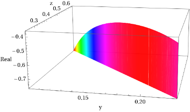
Figure 2: Real part of $\mathcal{O}(\epsilon^{0})_{\text{I}}$ for the process $S_{ggg}$

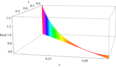
Figure 3: Real part of $\mathcal{O}(\epsilon^{1})_{\text{I}}$ for the process $S_{ggg}$

Figure 4: Real part of $\mathcal{O}(\epsilon^{2})_{\text{I}}$ for the process $S_{ggg}$

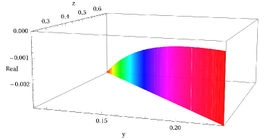
Figure 5: Real part of $\mathcal{O}(\epsilon^{0})_{\text{I}}$ for the process $S_{q\bar{q}g}$

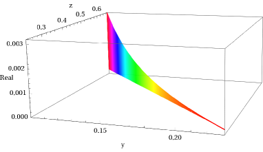
Figure 6: Real part of $\mathcal{O}(\epsilon^{1})_{\text{I}}$ for the process $S_{q\bar{q}g}$

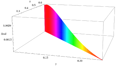
Figure 7: Real part of $\mathcal{O}(\epsilon^{2})_{\text{I}}$ for the process $S_{q\bar{q}g}$

VIII Summary

In this paper, we have analytically computed for the first time the matrix elements for the decay of a pseudo-scalar Higgs boson to $ggg$ and $q\bar{q}g$, which contribute beyond NNLO in QCD. Precisely we computed $\mathcal{O}(\epsilon^{3})$ and $\mathcal{O}(\epsilon^{4})$ at NLO and $\mathcal{O}(\epsilon^{1})$ and $\mathcal{O}(\epsilon^{2})$ amplitudes at NNLO, which contributes to a full three loop cross section for the processes under consideration. We have obtained these amplitudes by working in an effective theory with the heavy quark integrated out. The proper definition of $\gamma_{5}$ is essential in $d>4$ dimensions, and this fails to satisfy the Ward identity. In order to get back the renormalization invariance of the singlet axial current, a finite renormalization is needed. Using the renormalization constants $Z_{GG},Z_{GJ},Z_{JJ}$, we have obtained the $\mathcal{O}(\epsilon^{1})$ and $\mathcal{O}(\epsilon^{2})$ contributions at NNLO. We have checked our computation with the IR predictions from Catani Catani (1998), and found perfect agreement. In order to check our IR poles to the one from  Banerjee et al. (2017), we have analytically mapped the HPLs to GPLs, the resulting identities we have presented in our article. We have hugely simplified the analytical results with our in-house codes, which later helped for our numerical implementation. We have also checked our results at $\mathcal{O}(\epsilon^{0})$ with NNLO results calculated in Banerjee et al. (2017) and found perfect agreement. Keeping in mind that these amplitudes can form a part of some Monte Carlo codes, we have presented the numerical implementation of them, in FORTRAN-95 routines. In order to reduce the compilation time as well as to evaluate the amplitudes faster, we have optimised the results with FORM. The optimization of the matrix elements at different loops as well as different orders in $\epsilon$ presents different challenges, which we have discussed in detail in our article. We have discussed about our numerical implementation of the matrix elements, by evaluating them in different phase space regions. Our findings about the speed of evaluation per phase space points, beyond NNLO, are reported in Table 1. Finally, we provide the numerical implementations in FORTRAN-95 routines, which can be used with any Monte Carlo phase space generator. Our results will be important for the precise predictions of pseudo-scalar Higgs in association with a jet, beyond NNLO.

Appendix A

We recall here that the GPLs are defined as iterated integrals over the rational functions as,

$$G(l_{1},l_{2},...,l_{n};x)= \int_{0}^{x}\frac{dt}{t-l_{1}}~{}G(l_{2},...,l_{n};t),$$ (41)

$$G(\underbrace{0,0,..,0}_{n};x)= \frac{1}{n!}\text{ln}^{n}(x),~{}G(x)=1;$$ (42)

The definitions of the one and 2d-HPL for weight ($n$) one are:

$$H(1;y) = -\ln(1-y)\;,$$

$$H(0;y) = \ln y\;,$$

$$H(-1;y) = \ln(1+y)$$

$$H(1-z;y) = -\ln\left(1-\frac{y}{1-z}\right)\ ,$$

$$H(z;y) = \ln\left(\frac{y+z}{z}\right).$$ (43)

and the rational fractions for 1d-HPL

$$f(1;y)=\frac{1}{1-y}\;,f(0;y)=\frac{1}{y}\;,f(-1;y)=\frac{1}{1+y}\;,$$ (44)

For 2d-HPL, the rational fraction in terms of $y,z$

$$f(1-z;y)= \frac{1}{1-y-z}\;,~{}f(z;y)= \frac{1}{y+z}\;,$$ (45)

such that

$$\frac{\partial}{\partial y}H(a;y)=f(a;y),\;\\ \quad\mbox{with}\quad a=+1,0,-1,1-z,z.$$ (46)

For $n>1$:

$$H(0,\ldots,0;y) = \frac{1}{n!}\ln^{n}y\;,$$ (47)

$$H(a,\vec{b};y) = \int_{0}^{y}dtf(a;t)H(\vec{b};t)\;,$$ (48)

which satisfies the equation

$$\frac{\partial}{\partial y}H(a,\vec{b};y)=f(a;y)H(\vec{b};y)\;.$$ (49)

Appendix B

$$Z_{GG}= ~{}1+a_{s}\Bigg{[}\frac{1}{\epsilon}\Big{\{}\frac{22}{3}C_{A}-\frac{4}{3}n_{f}\Big{\}}\Bigg{]}+a_{s}^{2}\Bigg{[}\frac{1}{\epsilon^{2}}\Big{\{}\frac{484}{9}C_{A}^{2}-\frac{176}{9}C_{A}n_{f}+\frac{16}{9}n_{f}^{2}\Big{\}}+\frac{1}{\epsilon}\Big{\{}\frac{34}{3}C_{A}^{2}-\frac{10}{3}C_{A}n_{f}-2C_{F}n_{f}\Big{\}}\Bigg{]}$$ (50)

$$Z_{GJ}= ~{}a_{s}\Bigg{[}-\frac{24}{\epsilon}C_{F}\Bigg{]}+a_{s}^{2}\Bigg{[}\frac{1}{\epsilon^{2}}\Big{\{}-176C_{A}C_{F}+32C_{F}n_{f}\Big{\}}+\frac{1}{\epsilon}\Big{\{}-\frac{284}{3}C_{A}C_{F}+\frac{8}{3}C_{F}n_{f}+84C_{F}^{2}\Big{\}}\Bigg{]}$$ (51)

$$Z_{JJ}= ~{}1+a_{s}\Bigg{[}-4C_{F}\Bigg{]}+a_{s}^{2}\Bigg{[}\frac{1}{\epsilon}\Big{\{}\frac{44}{3}C_{A}C_{F}-\frac{10}{3}C_{F}n_{f}\Big{\}}-\frac{107}{9}C_{A}C_{F}+\frac{31}{18}C_{F}n_{f}+22C_{F}^{2}\Bigg{]}$$ (52)

References

- Aad et al. (2012) G. Aad et al. (ATLAS), Phys. Lett. B 716, 1 (2012), arXiv:1207.7214 [hep-ex] .
- Chatrchyan et al. (2012) S. Chatrchyan et al. (CMS), Phys. Lett. B 716, 30 (2012), arXiv:1207.7235 [hep-ex] .
- Aad et al. (2013) G. Aad et al. (ATLAS), Phys. Lett. B 726, 120 (2013), arXiv:1307.1432 [hep-ex] .
- Khachatryan et al. (2015) V. Khachatryan et al. (CMS), Phys. Rev. D 92, 012004 (2015), arXiv:1411.3441 [hep-ex] .
- Aad et al. (2020) G. Aad et al. (ATLAS), Eur. Phys. J. C 80, 957 (2020), [Erratum: Eur.Phys.J.C 81, 29 (2021), Erratum: Eur.Phys.J.C 81, 398 (2021)], arXiv:2004.03447 [hep-ex] .
- Sirunyan et al. (2020) A. M. Sirunyan et al. (CMS), Phys. Rev. Lett. 125, 061801 (2020), arXiv:2003.10866 [hep-ex] .
- Tumasyan et al. (2022) A. Tumasyan et al. (CMS), JHEP 06, 012 (2022), arXiv:2110.04836 [hep-ex] .
- Higgs (1964a) P. W. Higgs, Phys. Lett. 12, 132 (1964a).
- Higgs (1964b) P. W. Higgs, Phys. Rev. Lett. 13, 508 (1964b).
- Higgs (1966) P. W. Higgs, Phys. Rev. 145, 1156 (1966).
- Englert and Brout (1964) F. Englert and R. Brout, Phys. Rev. Lett. 13, 321 (1964).
- Guralnik et al. (1964) G. S. Guralnik, C. R. Hagen, and T. W. B. Kibble, Phys. Rev. Lett. 13, 585 (1964).
- Brein et al. (2013) O. Brein, R. V. Harlander, and T. J. E. Zirke, Comput. Phys. Commun. 184, 998 (2013), arXiv:1210.5347 [hep-ph] .
- Rainwater and Zeppenfeld (1997) D. L. Rainwater and D. Zeppenfeld, JHEP 12, 005 (1997), arXiv:hep-ph/9712271 .
- Rainwater et al. (1998) D. L. Rainwater, D. Zeppenfeld, and K. Hagiwara, Phys. Rev. D 59, 014037 (1998), arXiv:hep-ph/9808468 .
- Catani et al. (2023) S. Catani, S. Devoto, M. Grazzini, S. Kallweit, J. Mazzitelli, and C. Savoini, Phys. Rev. Lett. 130, 111902 (2023), arXiv:2210.07846 [hep-ph] .
- Agarwal et al. (2024) B. Agarwal, G. Heinrich, S. P. Jones, M. Kerner, S. Y. Klein, J. Lang, V. Magerya, and A. Olsson, JHEP 05, 013 (2024), [Erratum: JHEP 06, 142 (2024)], arXiv:2402.03301 [hep-ph] .
- de Florian et al. (1999) D. de Florian, M. Grazzini, and Z. Kunszt, Phys. Rev. Lett. 82, 5209 (1999), arXiv:hep-ph/9902483 .
- Ravindran et al. (2002) V. Ravindran, J. Smith, and W. L. Van Neerven, Nucl. Phys. B 634, 247 (2002), arXiv:hep-ph/0201114 .
- Dawson (1991) S. Dawson, Nucl. Phys. B 359, 283 (1991).
- Spira et al. (1995) M. Spira, A. Djouadi, D. Graudenz, and P. M. Zerwas, Nucl. Phys. B 453, 17 (1995), arXiv:hep-ph/9504378 .
- Harlander and Kilgore (2002) R. V. Harlander and W. B. Kilgore, JHEP 10, 017 (2002), arXiv:hep-ph/0208096 [hep-ph] .
- Anastasiou and Melnikov (2003) C. Anastasiou and K. Melnikov, Phys. Rev. D67, 037501 (2003), arXiv:hep-ph/0208115 [hep-ph] .
- Ravindran et al. (2003) V. Ravindran, J. Smith, and W. L. van Neerven, Nucl. Phys. B665, 325 (2003), arXiv:hep-ph/0302135 [hep-ph] .
- Graudenz et al. (1993) D. Graudenz, M. Spira, and P. M. Zerwas, Phys. Rev. Lett. 70, 1372 (1993).
- Spira et al. (1993) M. Spira, A. Djouadi, D. Graudenz, and P. M. Zerwas, Phys. Lett. B 318, 347 (1993).
- Kramer et al. (1998) M. Kramer, E. Laenen, and M. Spira, Nucl. Phys. B 511, 523 (1998), arXiv:hep-ph/9611272 .
- Czakon et al. (2021) M. Czakon, R. V. Harlander, J. Klappert, and M. Niggetiedt, Phys. Rev. Lett. 127, 162002 (2021), [Erratum: Phys.Rev.Lett. 131, 179901 (2023)], arXiv:2105.04436 [hep-ph] .
- Anastasiou et al. (2015) C. Anastasiou, C. Duhr, F. Dulat, F. Herzog, and B. Mistlberger, Phys. Rev. Lett. 114, 212001 (2015), arXiv:1503.06056 [hep-ph] .
- Mistlberger (2018) B. Mistlberger, JHEP 05, 028 (2018), arXiv:1802.00833 [hep-ph] .
- Anastasiou et al. (2016) C. Anastasiou, C. Duhr, F. Dulat, E. Furlan, T. Gehrmann, F. Herzog, A. Lazopoulos, and B. Mistlberger, JHEP 05, 058 (2016), arXiv:1602.00695 [hep-ph] .
- Chen et al. (2021) X. Chen, T. Gehrmann, E. W. N. Glover, A. Huss, B. Mistlberger, and A. Pelloni, Phys. Rev. Lett. 127, 072002 (2021), arXiv:2102.07607 [hep-ph] .
- Ahmed et al. (2014) T. Ahmed, M. Mahakhud, N. Rana, and V. Ravindran, Phys. Rev. Lett. 113, 112002 (2014), arXiv:1404.0366 [hep-ph] .
- Vogt et al. (2004) A. Vogt, S. Moch, and J. A. M. Vermaseren, Nucl. Phys. B691, 129 (2004), arXiv:hep-ph/0404111 [hep-ph] .
- Moch et al. (2004) S. Moch, J. A. M. Vermaseren, and A. Vogt, Nucl. Phys. B688, 101 (2004), arXiv:hep-ph/0403192 [hep-ph] .
- Haber and Kane (1985) H. E. Haber and G. L. Kane, Phys. Rept. 117, 75 (1985).
- Lane (1993) K. D. Lane, in Theoretical Advanced Study Institute (TASI 93) in Elementary Particle Physics: The Building Blocks of Creation - From Microfermius to Megaparsecs (1993) arXiv:hep-ph/9401324 .
- Arkani-Hamed et al. (1998) N. Arkani-Hamed, S. Dimopoulos, and G. R. Dvali, Phys. Lett. B 429, 263 (1998), arXiv:hep-ph/9803315 .
- Randall and Sundrum (1999) L. Randall and R. Sundrum, Phys. Rev. Lett. 83, 3370 (1999), arXiv:hep-ph/9905221 .
- Drees et al. (2004) M. Drees, R. Godbole, and P. Roy, Theory and Phenomenology of SParticles: an Account of Four-Dimensional N=1 Supersymmetry in High Energy Physics (2004).
- Fayet (1975) P. Fayet, Nucl. Phys. B 90, 104 (1975).
- Fayet (1976) P. Fayet, Phys. Lett. B 64, 159 (1976).
- Fayet (1977) P. Fayet, Phys. Lett. B 69, 489 (1977).
- Dimopoulos and Georgi (1981) S. Dimopoulos and H. Georgi, Nucl. Phys. B 193, 150 (1981).
- Sakai (1981) N. Sakai, Z. Phys. C 11, 153 (1981).
- Inoue et al. (1982a) K. Inoue, A. Kakuto, H. Komatsu, and S. Takeshita, Prog. Theor. Phys. 67, 1889 (1982a).
- Inoue et al. (1982b) K. Inoue, A. Kakuto, H. Komatsu, and S. Takeshita, Prog. Theor. Phys. 68, 927 (1982b), [Erratum: Prog.Theor.Phys. 70, 330 (1983)].
- Inoue et al. (1984) K. Inoue, A. Kakuto, H. Komatsu, and S. Takeshita, Prog. Theor. Phys. 71, 413 (1984).
- Kauffman and Schaffer (1994) R. P. Kauffman and W. Schaffer, Phys. Rev. D 49, 551 (1994), arXiv:hep-ph/9305279 .
- Ahmed et al. (2016a) T. Ahmed, M. C. Kumar, P. Mathews, N. Rana, and V. Ravindran, Eur. Phys. J. C 76, 355 (2016a), arXiv:1510.02235 [hep-ph] .
- Ahmed et al. (2016b) T. Ahmed, M. Bonvini, M. C. Kumar, P. Mathews, N. Rana, V. Ravindran, and L. Rottoli, Eur. Phys. J. C 76, 663 (2016b), arXiv:1606.00837 [hep-ph] .
- Ahmed et al. (2022) T. Ahmed, V. Ravindran, A. Sankar, and S. Tiwari, JHEP 01, 189 (2022), arXiv:2110.11476 [hep-ph] .
- Bhattacharya et al. (2020) A. Bhattacharya, M. Mahakhud, P. Mathews, and V. Ravindran, JHEP 02, 121 (2020), arXiv:1909.08993 [hep-ph] .
- Bozzi et al. (2006) G. Bozzi, S. Catani, D. de Florian, and M. Grazzini, Nucl. Phys. B 737, 73 (2006), arXiv:hep-ph/0508068 .
- Agarwal et al. (2018) N. Agarwal, P. Banerjee, G. Das, P. K. Dhani, A. Mukhopadhyay, V. Ravindran, and A. Tripathi, JHEP 12, 105 (2018), arXiv:1805.12553 [hep-ph] .
- Ravindran et al. (2024) V. Ravindran, A. Sankar, and S. Tiwari, Phys. Rev. D 110, 016019 (2024), arXiv:2309.14833 [hep-ph] .
- Banerjee et al. (2018) P. Banerjee, G. Das, P. K. Dhani, and V. Ravindran, Phys. Rev. D 97, 054024 (2018), arXiv:1708.05706 [hep-ph] .
- Chen et al. (2015) X. Chen, T. Gehrmann, E. W. N. Glover, and M. Jaquier, Phys. Lett. B740, 147 (2015), arXiv:1408.5325 [hep-ph] .
- Boughezal et al. (2013) R. Boughezal, F. Caola, K. Melnikov, F. Petriello, and M. Schulze, JHEP 06, 072 (2013), arXiv:1302.6216 [hep-ph] .
- Boughezal et al. (2015a) R. Boughezal, C. Focke, W. Giele, X. Liu, and F. Petriello, Phys. Lett. B 748, 5 (2015a), arXiv:1505.03893 [hep-ph] .
- Boughezal et al. (2015b) R. Boughezal, F. Caola, K. Melnikov, F. Petriello, and M. Schulze, Phys. Rev. Lett. 115, 082003 (2015b), arXiv:1504.07922 [hep-ph] .
- Caola et al. (2015) F. Caola, K. Melnikov, and M. Schulze, Phys. Rev. D 92, 074032 (2015), arXiv:1508.02684 [hep-ph] .
- Chen et al. (2016) X. Chen, J. Cruz-Martinez, T. Gehrmann, E. W. N. Glover, and M. Jaquier, JHEP 10, 066 (2016), arXiv:1607.08817 [hep-ph] .
- Campbell et al. (2019) J. M. Campbell, R. K. Ellis, and S. Seth, JHEP 10, 136 (2019), arXiv:1906.01020 [hep-ph] .
- Field et al. (2003) B. Field, J. Smith, M. E. Tejeda-Yeomans, and W. L. van Neerven, Phys. Lett. B 551, 137 (2003), arXiv:hep-ph/0210369 .
- Bernreuther et al. (2010) W. Bernreuther, P. Gonzalez, and M. Wiebusch, Eur. Phys. J. C 69, 31 (2010), arXiv:1003.5585 [hep-ph] .
- Kim and Williams (2024) Y. Kim and C. Williams, JHEP 08, 042 (2024), arXiv:2405.02210 [hep-ph] .
- Gehrmann et al. (2023) T. Gehrmann, P. Jakubčík, C. C. Mella, N. Syrrakos, and L. Tancredi, JHEP 04, 016 (2023), arXiv:2301.10849 [hep-ph] .
- Catani (1998) S. Catani, Phys. Lett. B427, 161 (1998), arXiv:hep-ph/9802439 [hep-ph] .
- Chetyrkin et al. (1998) K. G. Chetyrkin, B. A. Kniehl, M. Steinhauser, and W. A. Bardeen, Nucl. Phys. B535, 3 (1998), arXiv:hep-ph/9807241 [hep-ph] .
- Adler and Bardeen (1969) S. L. Adler and W. A. Bardeen, Phys. Rev. 182, 1517 (1969).
- ’t Hooft and Veltman (1972) G. ’t Hooft and M. J. G. Veltman, Nucl. Phys. B44, 189 (1972).
- Banerjee et al. (2017) P. Banerjee, P. K. Dhani, and V. Ravindran, JHEP 10, 067 (2017), arXiv:1708.02387 [hep-ph] .
- Nogueira (1993) P. Nogueira, J. Comput. Phys. 105, 279 (1993).
- Ruijl et al. (2017) B. Ruijl, T. Ueda, and J. Vermaseren, (2017), arXiv:1707.06453 [hep-ph] .
- Studerus (2010) C. Studerus, Comput. Phys. Commun. 181, 1293 (2010), arXiv:0912.2546 [physics.comp-ph] .
- von Manteuffel and Studerus (2012) A. von Manteuffel and C. Studerus, (2012), arXiv:1201.4330 [hep-ph] .
- Gehrmann and Remiddi (2001a) T. Gehrmann and E. Remiddi, Nucl. Phys. B 601, 287 (2001a), arXiv:hep-ph/0101124 .
- Gehrmann and Remiddi (2001b) T. Gehrmann and E. Remiddi, Nucl. Phys. B 601, 248 (2001b), arXiv:hep-ph/0008287 .
- Klappert et al. (2021) J. Klappert, F. Lange, P. Maierhöfer, and J. Usovitsch, Comput. Phys. Commun. 266, 108024 (2021), arXiv:2008.06494 [hep-ph] .
- Laporta (2000) S. Laporta, Int. J. Mod. Phys. A 15, 5087 (2000), arXiv:hep-ph/0102033 .
- Tkachov (1981) F. V. Tkachov, Phys. Lett. B100, 65 (1981).
- Chetyrkin and Tkachov (1981) K. G. Chetyrkin and F. V. Tkachov, Nucl. Phys. B192, 159 (1981).
- Gehrmann and Remiddi (2000) T. Gehrmann and E. Remiddi, Nucl. Phys. B580, 485 (2000), arXiv:hep-ph/9912329 [hep-ph] .
- Heller and von Manteuffel (2022) M. Heller and A. von Manteuffel, Comput. Phys. Commun. 271, 108174 (2022), arXiv:2101.08283 [cs.SC] .
- Tarasov et al. (1980) O. V. Tarasov, A. A. Vladimirov, and A. Yu. Zharkov, Phys. Lett. B93, 429 (1980).
- Larin (1993) S. A. Larin, Phys. Lett. B303, 113 (1993), arXiv:hep-ph/9302240 [hep-ph] .
- Trueman (1979) T. L. Trueman, Phys. Lett. B 88, 331 (1979).
- Zoller (2013) M. F. Zoller, JHEP 07, 040 (2013), arXiv:1304.2232 [hep-ph] .
- Ahmed et al. (2015) T. Ahmed, T. Gehrmann, P. Mathews, N. Rana, and V. Ravindran, JHEP 11, 169 (2015), arXiv:1510.01715 [hep-ph] .
- Sterman and Tejeda-Yeomans (2003) G. F. Sterman and M. E. Tejeda-Yeomans, Phys. Lett. B552, 48 (2003), arXiv:hep-ph/0210130 [hep-ph] .
- Becher and Neubert (2009) T. Becher and M. Neubert, Phys. Rev. Lett. 102, 162001 (2009), [Erratum: Phys. Rev. Lett.111,no.19,199905(2013)], arXiv:0901.0722 [hep-ph] .
- Korchemskaya and Korchemsky (1992) I. A. Korchemskaya and G. P. Korchemsky, Phys. Lett. B 287, 169 (1992).
- Korchemsky and Radyushkin (1987) G. P. Korchemsky and A. V. Radyushkin, Nucl. Phys. B 283, 342 (1987).
- Duhr and Dulat (2019) C. Duhr and F. Dulat, JHEP 08, 135 (2019), arXiv:1904.07279 [hep-th] .
- Kuipers et al. (2015) J. Kuipers, T. Ueda, and J. A. M. Vermaseren, Comput. Phys. Commun. 189, 1 (2015), arXiv:1310.7007 [cs.SC] .
- Kuipers et al. (2013) J. Kuipers, A. Plaat, J. A. M. Vermaseren, and H. J. van den Herik, Comput. Phys. Commun. 184, 2391 (2013), arXiv:1207.7079 [cs.SC] .
- Tentyukov and Vermaseren (2010) M. Tentyukov and J. A. M. Vermaseren, Comput. Phys. Commun. 181, 1419 (2010), arXiv:hep-ph/0702279 .
- Naterop et al. (2020) L. Naterop, A. Signer, and Y. Ulrich, Comput. Phys. Commun. 253, 107165 (2020), arXiv:1909.01656 [hep-ph] .