Outer-(ap)RAC Graphs
Abstract
An outer-RAC drawing of a graph is a straight-line drawing where all vertices are incident to the outer cell and all edge crossings occur at a right angle. If additionally, all crossing edges are either horizontal or vertical, we call the drawing outer-apRAC (ap for axis-parallel). A graph is outer-(ap)RAC if it admits an outer-(ap)RAC drawing. We investigate the class of outer-(ap)RAC graphs. We show that the outer-RAC graphs are a proper subset of the planar graphs with at most edges where is the number of vertices. This density bound is tight, even for outer-apRAC graphs. Moreover, we provide an SPQR-tree based linear-time algorithm which computes an outer-RAC drawing for every given series-parallel graph of maximum degree four. As a complementing result, we present planar graphs of maximum degree four and series-parallel graphs of maximum degree five that are not outer-RAC. Finally, for series-parallel graphs of maximum degree three we show how to compute an outer-apRAC drawing in linear time.
Keywords:
RAC, beyond planarity, density, series-parallel graphs1 Introduction
Crossings in graph drawings are well-known to impede readability. This fact was experimentally verified by Purchase [40] in 2000. Follow-up works showed that the topology and geometry of local crossing configurations are deciding factors in how large the impact of crossings on readability actually is. Crossings at larger crossing angles reduce readability to a lesser extent than those at smaller crossing angles [36, 37, 38]. These results gave rise to the research field graph drawing beyond planarity where graph drawings with specific requirements towards local crossing configurations have been considered. Substantial research has deepened our understanding of beyond-planar graphs; see [24, 35] for an overview.
In this paper, we consider right-angle-crossing drawings, or RAC drawings for short, which are straight-line drawings of graphs where every crossing occurs at a right angle. The RAC drawing model is directly motivated by empirical studies that gave rise to a deeper study of graph drawing beyond planarity [36, 37, 38]. Hence, it comes at no surprise, that RAC drawings have been thoroughly investigated. More precisely, a first theoretical study by Didimo et al. [23] established a linear edge density bound shortly after Huang’s initial eye tracking study [36]. In addition, they showed that every graph admits a RAC drawing with bends per edge [23] which was shown to be the tight number of bends by Arikushi et al. [7]. Subsequent works on RAC drawings considered edge density [1, 39, 44], area [28, 41], variants where edges are drawn as circular arcs [15], simultaneous RAC drawings [5, 11] and algorithms for restricted input graphs [2, 10, 16]. The complexity of the RAC drawing problem has first been shown to be NP-hard [6] and later to be -complete [42]; on the other hand, there are FPT algorithms parameterited by feedback edge number and by vertex cover number [14]. Recently, a variant of RAC drawings called axis-parallel RAC drawings, or apRAC drawings for short, was introduced, in which each crossing edge has slope [3]111Originally, the slopes where defined as and in [3]. We use the rotated version which will allow us to simplify our discussion in Section 5..
In beyond-planar graph drawing, a classical topic is to consider additional constraints for the drawings. One of these constraints is the outer drawing model where each vertex must be located on the outer cell of the drawing. Outer drawings may be utilized to visualize highly connected clusters in graphs [4, 32] which in real-world networks are often only sparsely connected to each other; see e.g. [29, 30]. Previous research has considered outer--planar [8, 12, 33, 34], outer-fanplanar [9, 13] and outer-confluent graphs [27]. Surprisingly however, the existing literature only considered outer-(ap)RAC drawings with additional constraints on the placement of vertices [18, 21] and for outer--planar graphs [17].
Our contribution.
We initiate the study of more general outer-(ap)RAC drawings in which vertices can be arbitrarily placed as long as they are incident to the outer cell. In the process, we prove that the outer-RAC graphs are a proper subfamily of the planar graphs in Section 3. Moreover, we show that certain planar graphs of low maximum degree do not admit outer-(ap)RAC drawings in Section 4. In contrast, we provide efficient outer-(ap)RAC drawing algorithms for series-parallel graphs of low maximum degree in Section 5. Finally, we conclude the paper with intriguing open questions.
2 Preliminaries
We assume familiarity with standard notation from graph theory, as found in [25] and basic graph drawing concepts, cf. [43]. In this paper, we consider all graphs to be simple. Let be a graph. A graph is said to be cubic, if all of its vertices have exactly degree . In a subcubic graph, every vertex has degree at most . The terms (sub)quartic are defined analogously for vertex degree . We call a drawing planar if in no two edges intersect except at a common endpoint. We say that a graph is planar if it admits a planar drawing. The connected regions of the plane in a planar drawing are called faces, the unbounded face is called outer face. A planar drawing in which each vertex is incident to the outer face is called outerplanar. If a graph admits an outerplanar drawing we call an outerplanar graph. In the weak dual graph of a planar drawing , each face except the outer face is represented by a vertex and faces are connected in if and only if and share an edge in . For an embedded outerplanar graph, the weak dual graph is a forest.
Similarly, the connected regions of the plane in a non-planar drawing are called cells and the unbounded cell is called outer cell. Consider a straight-line drawing , i.e., each edge is represented by a single segment. If in , all crossings occur at a right angle and all vertices are located on the outer cell, we call outer-RAC. If additionally, all crossing edges have slope , we call outer-apRAC. Moreover, we call a graph outer-(ap)RAC if it admits an outer-apRAC drawing.
An SPQR-tree of a graph describes a uniquely defined decomposition of according to its separation pairs [19, 20], which can be computed in linear time [31]. A node in is associated with a graph called the skeleton of which consists of virtual edges between the vertices of separation pairs in and at most one edge of . Each virtual edge corresponds to at least one path between its endpoints in . The pair of vertices separating the component represented by in are called the poles of . The vertices are connected by the parent virtual edge, which corresponds to a virtual edge in the parent of in . Based on the structure of its skeleton, a node is of one of four types:
-
•
S-node: forms a cycle of at least three virtual edges, including the parent virtual edge between and
-
•
P-node: is comprised of at least three parallel virtual edges between and one of which is the parent virtual edge
-
•
Q-node: contains the parent virtual edge and another edge between and , representing an actual edge in . If is the root of , the virtual edge of the skeleton instead corresponds to its unique child node .
-
•
R-node: is triconnected and contains the poles and . All its edges are virtual, the virtual edge between and is its parent virtual edge.
The SPQR-tree of a graph is by definition rooted at a -node. Moreover, all its leaves are -nodes. Also observe that two -nodes are never connected to each other and the same holds for two -nodes in . The subtree rooted at a node induces the so-called pertinent graph , which is a subgraph in obtained from merging the parent virtual edge in the skeleton of each node in the subtree of rooted at with the corresponding virtual edge in the skeleton of its respective parent node. A series-parallel graph, or short SP-graph, is a biconnected graph222In the literature there exists another recursive definition for series-parallel graphs [26]. However, one can obtain biconnectivity by a parallel composition with a single edge. whose SPQR-tree contains no -nodes. Since the skeleton of both P- and S-nodes are always planar, SP-graphs are always planar.
Lemma 1
Let be an SP-graph with vertices and let be its SQPR-tree rooted at any -node. Then, contains an -node such that all children of are -nodes.
Proof
If contains no -node the statement follows immediately. Otherwise, since all leaves of are -nodes, we find a -node by traversing top-down, such that the subtree of rooted at contains no other -node. By simplicity, has at most one -node child and hence at least one -node child whose children are all -nodes. ∎
We will make use of Lemma 1 to simplify the discussion of our algorithmic results in Section 5 as follows. Let be an -node such that all its children are -nodes in . We can now root at one of the -node children of , denoted as . After rerooting, we have that is the unique child of .
Corollary 1
Let be an SP-graph and be its SPQR-tree. can be rooted at a -node with unique child such that is an -node and at most one child of is a -node.
3 Topological Results
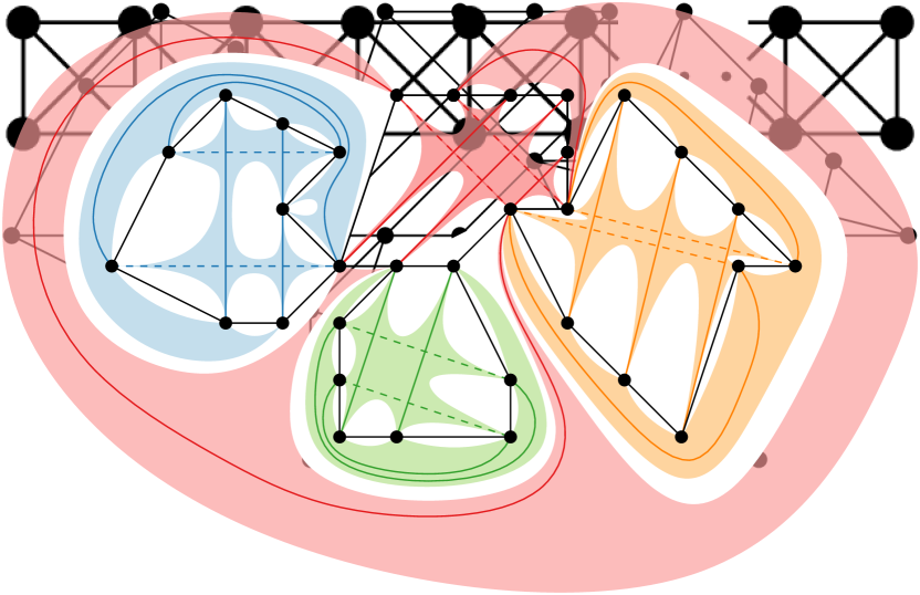
In this section, we provide some topological results. A useful tool for these results will be the notion of blocks of crossing edges in a given outer-RAC drawing of a graph . To this end, consider the crossing graph of which contains a vertex for each edge in and an edge if and only if and cross in . A block is any maximal connected vertex set in the transitive closure of ; see also Fig. 1. In particular, since in RAC drawings only edges drawn with perpendicular slopes cross, each block contains edges of only two perpendicular slopes. Thus, we can partition the edges of block obtaining slope sets with such that each pair of edges of for does not cross. Moreover, since we consider the outer-RAC setting, all endpoints of edges of the same block are located on the outer face. Since in addition, edges assigned to different blocks do not cross by definition, we can cover the interior of a RAC drawing with regions called outlines of blocks that contain all crossing edges as follows. Consider a block . Sort the endpoints of the edges in according to their occurrence in a clockwise cyclic walk along the outer face of and enumerate them by . Then, there necessarily exists a closed cycle , called the outline of , such that 1. is disjoint from the interior of (in other words, each point is either inside a bounded cell of or on the boundary of ), 2. does not cross any edges except at their endpoints, 3. contains all edges of but no other edge of , and 4. traverses in order. More precisely, when traversing along from to , one can follow the clockwise last333When considering the edges incident to in clockwise order starting from the direction in which we reach along coming from . edge of incident to up to its first crossing and then following the edge encountered up to its next crossing where we again follow the crossing edge; see also Fig. 1(a). Necessarily, due to the fact that the drawing is outer-RAC, a repeated application of this method will finish at .

Theorem 3.1
Let be an outer-RAC graph. Then is planar.
Proof
Consider any outer-RAC drawing of . We will describe how to obtain a planar drawing of . First, extend by all the outlines of blocks obtaining a drawing . By construction, is still bounded by the outer cycle which contains all vertices. Moreover, the outlines of blocks do not cross each other by construction. We now copy the interior of to the outside. Observe that in this copying operation we disregard the geometry but maintain the topology of the drawing. We now have two copies of each edge, each staying within its respective block outline either in the interior or the exterior of . For each block , consider now the slope sets and . We will remove the copies of in the interior of and the copies of in the exterior of . Since edges of the same slope set do not cross, we obtain a planar drawing of by removing the block outlines; see Fig. 1(b) for an illustration. ∎
One may wonder if in fact every planar graph is also outer-RAC. We will show that this is not the case by providing a density upper bound for outer-RAC graphs. As an intermediate step, we consider a special subclass of outer-RAC graphs. We call a graph bounded block graph if it can be partitioned into a Hamiltonian cycle and a set of edges and admits a bounded block drawing , that is, a drawing where 1. each edge of is drawn straight-line and crosses only at right angles, 2. forms the crossing-free outer boundary of and is not necessarily drawn straight-line, and 3. all edges of belong to a single block.
Lemma 2
Let be a bounded block graph with vertices. Then, has at most edges.
Proof
Let be a bounded block drawing of . The crossing edges of form a block that can be partitioned into two slope sets and . In addition, contains only the plane cycle which is topologically equivalent to the outline . We now consider for the subgraph of induced by the edges of and . Recall, that all edges of are parallel, i.e., is an embedded outerplanar subgraph of . We simplify obtaining by replacing each maximal path of edges of on the boundary of the same internal face by a single edge unless this creates a parallel edge with an edge of in which case we replace by a path of length . Hence, each internal face of contains exactly edges not belonging to . We claim that for each internal face of length , we can assign triangular faces. To this end, recall that the weak dual graph that has a vertex for each internal face and an edge between faces sharing an edge is in fact a forest. Since each edge of necessarily is part of two faces, has degree in . Moreover, each triangular face has only one edge of , i.e., degree in . Thus, such an assignment is possible in such a way that two triangular faces , remain unassigned. We now root at and count the number of vertices and edges in an in-order processing of .
At the root, we encounter vertices and edges. If we encounter another face , it shares vertices and edge with its parent. That is, if the face has length with , we find additional vertices and additional edges. Thus, writing for the number of faces of length , we obtain the number of vertices and edges of :
| (1) | ||||
| (2) |
The additive constants refer to faces and whereas in the sum expressions we add both the vertices of faces of length as well as the assigned triangular faces.
We can now transfer back to an accounting for graph by subdividing the edges replacing paths of non-crossed edges suitably. Each such subdivision creates another edge and another vertex. Writing for the number of such subdivisions and and for the number of vertices and edges of , respectively, we can refine (1) and (2) as follows:
| (3) | ||||
| (4) |
Now we compute the number of edges of . Necessarily, we have . Moreover, both and contain the outer cycle on vertices. Thus,
| (5) |
Theorem 3.2 ()
Let be an outer-RAC graph with vertices. Then, it has at most edges. Moreover, if has exactly edges, it can be decomposed into bounded blocks such that for 1. shares exactly one edge with the subgraph induced by , 2. is isomorphic to .
Proof (Sketch of Proof)
We investigate any outer-RAC drawing of . We first augment by inserting all outlines of blocks defined by and by triangulating the faces bounded only by crossing-free edges. We obtain a supergraph with an associated drawing , in which all crossing edges are straight-line. Then, we observe that can be obtained starting from a bounded block graph by an iterative procedure. In each step, we have a graph and obtain by merging with a new bounded block graph either at a single vertex or at an edge. Finally, we show inductively that in this procedure the upper bound on the number of edges holds. See Appendix 0.A for details. ∎
Theorem 3.2 already also describes a potential matching density lower bound. In fact, the existing literature already establishes that it is indeed outer-RAC. Namely, Dehkordi and Eades proved that every outer--planar graph is also outer-RAC [17] whereas Didimo [22] and Auer et al. [8] independently found a lower bound of edges for outer--planar graphs. Here we strengthen their result by explicitly noting that it generalizes to outer-apRAC.
Theorem 3.3 ([8, 17, 22])
There is an infinitely large family of outer-apRAC graphs with vertices and edges.


Proof
is clearly outer-apRAC, e.g., place the four vertices at coordinates , , and . Since the outer cycle of this drawing is square-shaped, we can form a chain of such ’s by identifying the left edge of a copy with the right edge of another one; see Fig. 2(a). In this drawing, only edges of slopes and cross and all vertices are on the outer face, i.e., it is outer-apRAC. ∎
Also note that the edge density bound differs from a tight bound of for circular RAC drawings, in which all vertices are constrained to lie on a circle [18].
4 Obstructions for Outer-RAC Graphs
Theorem 3.2 already provides examples of planar graphs that admit no outer-RAC drawings. In this section, we provide planar graphs that admit no outer-RAC drawing despite being of low enough density. To this end, we first observe that parallel short paths admit only a few specific topologies in outer-RAC drawings.
Lemma 3
Let be a graph consisting of two paths and with . Then, in any outer-RAC drawing , and are not self-intersecting and one of the following holds:
-
P2.1
, , and occur in this order along the outer cycle of . Moreover, and do not intersect.
-
P2.2
, , and occur in this order along the outer cycle of . Moreover, and intersect exactly once at edges and .
-
P2.3
, , and occur in this order along the outer cycle of . Moreover, and intersect exactly once at edges and .
Proof
First, observe that each of and cannot cross itself as and each contain only two straight-line edges that share an endpoint.
In the following, assume that we already have an outer-RAC drawing of . We investigate how can be added while maintaining that the drawing is outer-RAC. First, if and do not cross, we arrive at the configuration described in Case P2.1. Second, assume that and cross. Since the pairs of edges and share a common endpoint, they cannot cross each other. Hence, only edge pairs and may cross. If exactly one of these edge pairs cross, we arrive at one of Cases P2.2 and P2.3.
Hence, it remains to consider the case where and as well as and cross. Assume that this is possible. Since and cross, we have that , , and either occur in this order around the outer cycle of or in the reversed order , , and . We assume w.l.o.g. that the order is , , and . Now, observe that and are separated by at least one vertex in both orientations of the outer cycle of . Since must cross , adding it removes at least one vertex from the outer cycle (see Fig. 2(b)); a contradiction. ∎
For three such short paths, we obtain yet a different result:
Lemma 4
Let be a graph consisting of three paths , and with , and . Then, in any outer-RAC drawing , , and are not self-intersecting, two paths, say and , cross, whereas is crossing-free, and one of the following holds:
-
P3.1
, , , and occur in this order along the outer cycle of . Moreover, and intersect exactly once at edges and .
-
P3.2
, , , and occur in this order along the outer cycle of . Moreover, and intersect exactly once at edges and .
Moreover, if is subgraph of an outer-RAC graph , and are not crossed by any edge not belonging to .
Proof
Consider any outer-RAC drawing of . Using Lemma 3, we know that each pair of paths can only be realized in three different ways. First note that necessarily two paths must cross as otherwise and form a cycle that w.l.o.g. contains ; i.e., is not on the outer cycle.
Thus, w.l.o.g. and cross according to Case P2.2 of Lemma 3 (Case P2.3 is symmetric) and let denote the point where and cross. Assume for a contradiction that any edge not belonging to or crosses }. Note that may be part of or of a supergraph of . First, since is RAC, cannot cross at . Next, observe that and induce two triangular regions and which have a right angle at ; see Fig. 2(c). Moreover, all edges of and are entirely on the boundary of and . That is, if intersects an edge of or , it is partially located inside . In fact, the edge that intersects must cross twice as none of its endpoints can be located in as then it would not be on the outer face. However, because is triangular, it contains no two parallel bounding segments; a contradiction.
Theorem 4.1
There is a SP-graph of maximum degree that is not outer-RAC.
Proof
Consider the graph . It is a parallel composition of five paths of length , i.e., it is series-parallel. By Lemma 4, it follows directly that it cannot admit an outer-RAC drawing. ∎
Theorem 4.2
There is a planar triconnected graph of maximum degree that is not outer-RAC.
Proof
Consider the octahedral graph . It consists of a composed of four parallel short paths , , and and a cycle on . By Lemma 4, in any of the outer-RAC drawings of , w.l.o.g. we have that its vertices occur in the order along the outer cycle of . Since there is a cycle on present in , is adjacent to . Clearly, edge must cross the drawing of the as otherwise or cannot be on the outer cycle. But then, crosses which, by Lemma 4, is already crossed by edge ; a contradiction. ∎
In particular, Theorems 4.1 and 4.2 motivate us to study SP-graphs of maximum degree four. Namely, SP-graphs are exactly the planar graphs that contain no subdivision of triconnected graphs, whereas our counterexamples for SP-graphs are of maximum degree five. In Section 5, we will provide drawing algorithms for such graphs that draw the graph according to its SPQR-tree in a top-down fashion. In particular, for S-nodes, we will realize the skeleton without crossings. In Appendix 0.B, we show that this may not be guaranteed for maximum degree four SP-graphs if we restrict the drawings to be outer-apRAC.
5 Outer-RAC Drawings for Bounded Degree SP-Graphs
Theorem 5.1
Let be a biconnected SP-graph with maximum degree . An outer-apRAC drawing of can be computed in time.
Proof
Let be a subcubic biconnected SP-graph and be its SPQR-tree, hence contains no -nodes. In order to construct the outer-apRAC drawing of , we perform a top-down pre-order visit of and draw the skeleton of each visited node depending on its type. Let be the vertex currently processed. We draw the virtual edges of corresponding to child nodes of . In this process, we also place the poles of its children, and , . Also, when we draw the parent virtual edge corresponding to a node , we define a reserved region , in which we will draw the skeleton of (aside from and ) later. More precisely, is defined as the intersection of three half planes, one being the closed half plane left of a line through the poles and of with lying above , the second being the open half plane below a horizontal line through and the third being the open half plane above a horizontal line through ; see Fig. 3(a) for an illustration. Further, we maintain the following invariants:
-
I.1
Virtual edges in of an already processed node that correspond to a not yet processed child node of are drawn vertically.
-
I.2
Let be a not yet processed non--node whose parent node in has been processed. Then is free, i.e., it contains only the edge .
-
I.3
All crossing edges cross at right angles and have either slope or .
-
I.4
Every already drawn vertex is incident to the outer cell.


Initialization.
Observe that if contains no -node, is a cycle and therefore outerplanar and thus also outer-apRAC. Hence in the following, we can assume that contains at least one -node. We then root according to Corollary 1; see Fig. 3(b). Now, the root has as a child an -node which in turn has exactly one -node child . In , according to the skeleton of , we have that and the -node children of form a path connecting the poles of . As contains at least two edges ( and at least one -node child of ) we draw the path such that the poles of are vertically aligned as depicted in Fig. 3(c), maintaining I.1 for the virtual edge corresponding to . As there are no crossings and is drawn outside of , I.2, I.3 and I.4 are guaranteed.
Next, we show how to handle a non-root node in the top-down traversal of .
is a -node.
is a -node.
Since is subcubic, has exactly two child nodes in , where each is either of type or type . Moreover, according to I.1, is a vertical segment and is free according to I.2. While processing , we will partially draw the pertinent graph of each -node child and remove the drawn edges from its skeleton. The remaining edges of the respective -node child are then drawn in the recursive case. First, assume that has a single -node child and a -node child . Then the virtual edges and are -nodes, due to the maximum vertex degree. We delete and from and reassign the poles to and to . If the modified is empty, we simply draw and inside the free region . Otherwise, the edges and are then drawn as depicted in Fig. 4(a) within . Further, we add a virtual edge to which represents the modified node . The reserved region of is defined as and free as it is a subset of . For , the reference edge is which is already drawn vertically. Hence, we maintain I.1, I.2, I.3 and I.4.
Second, consider the case that has two -node children and . By the maximum vertex degree, the virtual edges in and incident to and correspond to -node children of and of . Further, let be the virtual edge in corresponding to , such that and . We remove the edges from and redefine the poles as and as . Similarly, we remove from such that and . Next, we draw the edges inside such that crosses while are drawn crossing-free. Moreover, is drawn at slope and at slope . If the skeleton of is not empty after its modification, we insert a vertical virtual edge for the remainder of and define the reserved region which is free as it is a subset of . Similarly, we add a vertical virtual edge if is non-empty and define its reserved region which again is free as it also is a subset of . See Fig. 4(b) for the construction. Otherwise, the crossing-free edges are drawn as shown in Fig. 4(c) inside . The inserted virtual edges and the respective reserved regions clearly fulfill I.1 and I.2, while all other drawn edges correspond to real edges in and are not considered in the subsequent processing of . The only crossing is the one of and , which maintains I.3. Due to this crossing, all vertices are incident to the outer cell, guaranteeing I.4.


is a -node.
consists of a path of virtual edges from to . and were already placed when processing the parent node in such that is a vertical segment by I.1. Let be the virtual edge corresponding to child node . We draw as equally sized, consecutive vertical lines between and , maintaining I.1 and I.4. It follows that which is free by I.2 is vertically divided into equally sized sub-regions; see Fig. 4(d). As the reserved regions only share common borders and are located inside , I.2 is guaranteed. As there are no crossings, I.3 is maintained.
Correctness.
For a parent virtual edge corresponding to a not yet drawn node , the endpoints are the poles . Thus, I.1 ensures that the reserved region is well defined. Further, I.2 guarantees that there is no overlap between different parts of the drawing, as the skeleton of each node is drawn within and each child of gets a free area that is part of as described above. Since reserved regions of sibling nodes do not overlap, all occurring crossings in are drawn explicitly in our algorithm and I.3 ensures that they are right-angled and have the same slope. Finally, all vertices in are incident to the outer face by I.4. As I.1 to I.4 are maintained, the resulting drawing is outer-apRAC.
Running time.
We construct in linear time due to [31]. As there are operations per node, the top-down visit is in , resulting in time. ∎
Using similar but more sophisticated techniques we prove in Appendix 0.C:
Theorem 5.2 ()
Let be a biconnected SP-graph with maximum degree . An outer-RAC drawing of can be computed in time.
6 Open Problems
We conjecture that all subcubic planar graphs and all subquartic SP-graphs are outer-apRAC. For the first conjecture, one needs to draw triconnected subcubic planar graphs whereas for the second one we need a technique for S-nodes that introduces crossings in certain cases. Also, we believe that a high vertex degree at any vertex is also an obstruction for outer-RAC; such a property may be useful for a full characterization. Moreover, an efficient recognition algorithm for general SP- or planar graphs is of interest as well as an area-efficient drawing algorithm for subquartic SP-graphs. To this end note that our drawing algorithms produce exponential-area drawings. Finally, Theorem 3.1 motivates to study outer-RAC drawings where edges have bends or are drawn with circular arcs [15]. To this end, also note that every graph is outer-apRAC with three bends per edge [23].
References
- [1] Angelini, P., Bekos, M.A., Förster, H., Kaufmann, M.: On RAC drawings of graphs with one bend per edge. Theor. Comput. Sci. 828-829, 42–54 (2020). https://doi.org/10.1016/J.TCS.2020.04.018, https://doi.org/10.1016/j.tcs.2020.04.018
- [2] Angelini, P., Bekos, M.A., Katheder, J., Kaufmann, M., Pfister, M.: RAC drawings of graphs with low degree. In: Szeider, S., Ganian, R., Silva, A. (eds.) 47th Int. Symp. on Mathematical Foundations of Computer Science, MFCS 2022. LIPIcs, vol. 241, pp. 11:1–11:15. Schloss Dagstuhl - Leibniz-Zentrum für Informatik (2022). https://doi.org/10.4230/LIPICS.MFCS.2022.11, https://doi.org/10.4230/LIPIcs.MFCS.2022.11
- [3] Angelini, P., Bekos, M.A., Katheder, J., Kaufmann, M., Pfister, M., Ueckerdt, T.: Axis-parallel right angle crossing graphs. In: Gørtz, I.L., Farach-Colton, M., Puglisi, S.J., Herman, G. (eds.) 31st Annual European Symposium on Algorithms, ESA 2023. LIPIcs, vol. 274, pp. 9:1–9:15. Schloss Dagstuhl - Leibniz-Zentrum für Informatik (2023). https://doi.org/10.4230/LIPICS.ESA.2023.9, https://doi.org/10.4230/LIPIcs.ESA.2023.9
- [4] Angori, L., Didimo, W., Montecchiani, F., Pagliuca, D., Tappini, A.: Hybrid graph visualizations with chordlink: Algorithms, experiments, and applications. IEEE Trans. Vis. Comput. Graph. 28(2), 1288–1300 (2022). https://doi.org/10.1109/TVCG.2020.3016055, https://doi.org/10.1109/TVCG.2020.3016055
- [5] Argyriou, E.N., Bekos, M.A., Kaufmann, M., Symvonis, A.: Geometric RAC simultaneous drawings of graphs. J. Graph Algorithms Appl. 17(1), 11–34 (2013). https://doi.org/10.7155/JGAA.00282, https://doi.org/10.7155/jgaa.00282
- [6] Argyriou, E.N., Bekos, M.A., Symvonis, A.: The straight-line RAC drawing problem is NP-hard. J. Graph Algorithms Appl. 16(2), 569–597 (2012). https://doi.org/10.7155/JGAA.00274, https://doi.org/10.7155/jgaa.00274
- [7] Arikushi, K., Fulek, R., Keszegh, B., Moric, F., Tóth, C.D.: Graphs that admit right angle crossing drawings. Comput. Geom. 45(4), 169–177 (2012). https://doi.org/10.1016/J.COMGEO.2011.11.008, https://doi.org/10.1016/j.comgeo.2011.11.008
- [8] Auer, C., Bachmaier, C., Brandenburg, F.J., Gleißner, A., Hanauer, K., Neuwirth, D., Reislhuber, J.: Outer 1-planar graphs. Algorithmica 74(4), 1293–1320 (2016). https://doi.org/10.1007/S00453-015-0002-1, https://doi.org/10.1007/s00453-015-0002-1
- [9] Bekos, M.A., Cornelsen, S., Grilli, L., Hong, S., Kaufmann, M.: On the recognition of fan-planar and maximal outer-fan-planar graphs. Algorithmica 79(2), 401–427 (2017). https://doi.org/10.1007/S00453-016-0200-5, https://doi.org/10.1007/s00453-016-0200-5
- [10] Bekos, M.A., Didimo, W., Liotta, G., Mehrabi, S., Montecchiani, F.: On RAC drawings of 1-planar graphs. Theor. Comput. Sci. 689, 48–57 (2017). https://doi.org/10.1016/J.TCS.2017.05.039, https://doi.org/10.1016/j.tcs.2017.05.039
- [11] Bekos, M.A., van Dijk, T.C., Kindermann, P., Wolff, A.: Simultaneous drawing of planar graphs with right-angle crossings and few bends. J. Graph Algorithms Appl. 20(1), 133–158 (2016). https://doi.org/10.7155/JGAA.00388, https://doi.org/10.7155/jgaa.00388
- [12] Biedl, T.: Drawing outer-1-planar graphs revisited. J. Graph Algorithms Appl. 26(1), 59–73 (2022). https://doi.org/10.7155/JGAA.00581, https://doi.org/10.7155/jgaa.00581
- [13] Binucci, C., Di Giacomo, E., Didimo, W., Montecchiani, F., Patrignani, M., Symvonis, A., Tollis, I.G.: Fan-planarity: Properties and complexity. Theor. Comput. Sci. 589, 76–86 (2015). https://doi.org/10.1016/J.TCS.2015.04.020, https://doi.org/10.1016/j.tcs.2015.04.020
- [14] Brand, C., Ganian, R., Röder, S., Schager, F.: Fixed-parameter algorithms for computing RAC drawings of graphs. In: Bekos, M.A., Chimani, M. (eds.) 31st Int. Symp. on Graph Drawing and Network Visualization, GD 2023. Lecture Notes in Computer Science, vol. 14466, pp. 66–81. Springer (2023). https://doi.org/10.1007/978-3-031-49275-4_5, https://doi.org/10.1007/978-3-031-49275-4_5
- [15] Chaplick, S., Förster, H., Kryven, M., Wolff, A.: Drawing graphs with circular arcs and right-angle crossings. In: Albers, S. (ed.) 17th Scandinavian Symposium and Workshops on Algorithm Theory, SWAT 2020. LIPIcs, vol. 162, pp. 21:1–21:14. Schloss Dagstuhl - Leibniz-Zentrum für Informatik (2020). https://doi.org/10.4230/LIPICS.SWAT.2020.21, https://doi.org/10.4230/LIPIcs.SWAT.2020.21
- [16] Chaplick, S., Lipp, F., Wolff, A., Zink, J.: Compact drawings of 1-planar graphs with right-angle crossings and few bends. Comput. Geom. 84, 50–68 (2019). https://doi.org/10.1016/J.COMGEO.2019.07.006, https://doi.org/10.1016/j.comgeo.2019.07.006
- [17] Dehkordi, H.R., Eades, P.: Every outer-1-plane graph has a right angle crossing drawing. Int. J. Comput. Geom. Appl. 22(6), 543–558 (2012). https://doi.org/10.1142/S021819591250015X, https://doi.org/10.1142/S021819591250015X
- [18] Dehkordi, H.R., Eades, P., Hong, S., Nguyen, Q.H.: Circular right-angle crossing drawings in linear time. Theor. Comput. Sci. 639, 26–41 (2016). https://doi.org/10.1016/J.TCS.2016.05.017, https://doi.org/10.1016/j.tcs.2016.05.017
- [19] Di Battista, G., Tamassia, R.: On-line maintenance of triconnected components with SPQR-trees. Algorithmica 15(4), 302–318 (1996). https://doi.org/10.1007/BF01961541, https://doi.org/10.1007/BF01961541
- [20] Di Battista, G., Tamassia, R.: On-line planarity testing. SIAM J. Comput. 25(5), 956–997 (1996). https://doi.org/10.1137/S0097539794280736, https://doi.org/10.1137/S0097539794280736
- [21] Di Giacomo, E., Didimo, W., Eades, P., Liotta, G.: 2-layer right angle crossing drawings. Algorithmica 68(4), 954–997 (2014). https://doi.org/10.1007/S00453-012-9706-7, https://doi.org/10.1007/s00453-012-9706-7
- [22] Didimo, W.: Density of straight-line 1-planar graph drawings. Inf. Process. Lett. 113(7), 236–240 (2013). https://doi.org/10.1016/J.IPL.2013.01.013, https://doi.org/10.1016/j.ipl.2013.01.013
- [23] Didimo, W., Eades, P., Liotta, G.: Drawing graphs with right angle crossings. Theor. Comput. Sci. 412(39), 5156–5166 (2011). https://doi.org/10.1016/J.TCS.2011.05.025, https://doi.org/10.1016/j.tcs.2011.05.025
- [24] Didimo, W., Liotta, G., Montecchiani, F.: A survey on graph drawing beyond planarity. ACM Comput. Surv. 52(1), 4:1–4:37 (2019). https://doi.org/10.1145/3301281, https://doi.org/10.1145/3301281
- [25] Diestel, R.: Graph Theory, 5th Edition, Graduate texts in mathematics, vol. 173. Springer (2012)
- [26] Eppstein, D.: Parallel recognition of series-parallel graphs. Inf. Comput. 98(1), 41–55 (1992). https://doi.org/10.1016/0890-5401(92)90041-D, https://doi.org/10.1016/0890-5401(92)90041-D
- [27] Förster, H., Ganian, R., Klute, F., Nöllenburg, M.: On strict (outer-)confluent graphs. J. Graph Algorithms Appl. 25(1), 481–512 (2021). https://doi.org/10.7155/JGAA.00568, https://doi.org/10.7155/jgaa.00568
- [28] Förster, H., Kaufmann, M.: On compact RAC drawings. In: Grandoni, F., Herman, G., Sanders, P. (eds.) 28th Annual European Symposium on Algorithms, ESA 2020. LIPIcs, vol. 173, pp. 53:1–53:21. Schloss Dagstuhl - Leibniz-Zentrum für Informatik (2020). https://doi.org/10.4230/LIPICS.ESA.2020.53, https://doi.org/10.4230/LIPIcs.ESA.2020.53
- [29] Fortunato, S.: Community detection in graphs. Physics Reports 486(3), 75–174 (2010). https://doi.org/https://doi.org/10.1016/j.physrep.2009.11.002, https://www.sciencedirect.com/science/article/pii/S0370157309002841
- [30] Girvan, M., Newman, M.E.J.: Community structure in social and biological networks. Proceedings of the National Academy of Sciences 99(12), 7821–7826 (2002). https://doi.org/10.1073/pnas.122653799, https://www.pnas.org/doi/abs/10.1073/pnas.122653799
- [31] Gutwenger, C., Mutzel, P.: A linear time implementation of SPQR-trees. In: Marks, J. (ed.) 8th Int. Symp. on Graph Drawing, GD 2000. Lecture Notes in Computer Science, vol. 1984, pp. 77–90. Springer (2000). https://doi.org/10.1007/3-540-44541-2_8, https://doi.org/10.1007/3-540-44541-2_8
- [32] Henry, N., Fekete, J., McGuffin, M.J.: Nodetrix: a hybrid visualization of social networks. IEEE Trans. Vis. Comput. Graph. 13(6), 1302–1309 (2007). https://doi.org/10.1109/TVCG.2007.70582, https://doi.org/10.1109/TVCG.2007.70582
- [33] Hong, S., Eades, P., Katoh, N., Liotta, G., Schweitzer, P., Suzuki, Y.: A linear-time algorithm for testing outer-1-planarity. Algorithmica 72(4), 1033–1054 (2015). https://doi.org/10.1007/S00453-014-9890-8, https://doi.org/10.1007/s00453-014-9890-8
- [34] Hong, S., Nagamochi, H.: Testing full outer-2-planarity in linear time. In: Mayr, E.W. (ed.) 41st Int. Workshop on Graph-Theoretic Concepts in Computer Science, WG 2015. Lecture Notes in Computer Science, vol. 9224, pp. 406–421. Springer (2015). https://doi.org/10.1007/978-3-662-53174-7_29, https://doi.org/10.1007/978-3-662-53174-7_29
- [35] Hong, S., Tokuyama, T. (eds.): Beyond Planar Graphs, Communications of NII Shonan Meetings. Springer (2020). https://doi.org/10.1007/978-981-15-6533-5, https://doi.org/10.1007/978-981-15-6533-5
- [36] Huang, W.: Using eye tracking to investigate graph layout effects. In: Hong, S., Ma, K. (eds.) APVIS 2007, 6th International Asia-Pacific Symposium on Visualization 2007. pp. 97–100. IEEE Computer Society (2007). https://doi.org/10.1109/APVIS.2007.329282, https://doi.org/10.1109/APVIS.2007.329282
- [37] Huang, W., Eades, P., Hong, S.: Larger crossing angles make graphs easier to read. J. Vis. Lang. Comput. 25(4), 452–465 (2014). https://doi.org/10.1016/J.JVLC.2014.03.001, https://doi.org/10.1016/j.jvlc.2014.03.001
- [38] Huang, W., Hong, S., Eades, P.: Effects of crossing angles. In: IEEE VGTC Pacific Visualization Symposium 2008, PacificVis 2008. pp. 41–46. IEEE Computer Society (2008). https://doi.org/10.1109/PACIFICVIS.2008.4475457, https://doi.org/10.1109/PACIFICVIS.2008.4475457
- [39] Kaufmann, M., Klemz, B., Knorr, K., Reddy, M.M., Schröder, F., Ueckerdt, T.: The density formula: One lemma to bound them all. CoRR abs/2311.06193 (2023). https://doi.org/10.48550/ARXIV.2311.06193, https://doi.org/10.48550/arXiv.2311.06193
- [40] Purchase, H.C.: Effective information visualisation: a study of graph drawing aesthetics and algorithms. Interact. Comput. 13(2), 147–162 (2000). https://doi.org/10.1016/S0953-5438(00)00032-1, https://doi.org/10.1016/S0953-5438(00)00032-1
- [41] Rahmati, Z., Emami, F.: RAC drawings in subcubic area. Inf. Process. Lett. 159-160, 105945 (2020). https://doi.org/10.1016/J.IPL.2020.105945, https://doi.org/10.1016/j.ipl.2020.105945
- [42] Schaefer, M.: RAC-drawability is -complete and related results. J. Graph Algorithms Appl. 27(9), 803–841 (2023). https://doi.org/10.7155/JGAA.00646, https://doi.org/10.7155/jgaa.00646
- [43] Tamassia, R. (ed.): Handbook on Graph Drawing and Visualization. Chapman and Hall/CRC (2013), https://www.crcpress.com/Handbook-of-Graph-Drawing-and-Visualization/Tamassia/9781584884125
- [44] Tóth, C.D.: On RAC drawings of graphs with two bends per edge. In: Bekos, M.A., Chimani, M. (eds.) 31st Int. Symp. on Graph Drawing and Network Visualization, GD 2023. Lecture Notes in Computer Science, vol. 14465, pp. 69–77. Springer (2023). https://doi.org/10.1007/978-3-031-49272-3_5, https://doi.org/10.1007/978-3-031-49272-3_5
Appendix 0.A Proof of Theorem 3.2
See 3.2
Proof
Consider any outer-RAC drawing of . We assume w.l.o.g. that is connected, otherwise, we can connect the single components in a treelike structure by adding edges. We extend by all the outlines of blocks and then triangulate all faces bounded by crossing-free edges to obtain a drawing of a supergraph of where outlines are interpreted as cycles of edges. This may introduce parallel edges and self-loops. We will show now that the cycle formed by two parallel edges and is necessarily empty of other edges and vertices, i.e., we can remove or from . To this end, note that at least one of and , say must be part of an outline boundary. Assume for a contradiction that for some block . Since , we have that is crossed by an edge of such that occur in this order along the outer boundary of . Since is located inside , it must cross , a contradiction. Thus, we have and for two distinct blocks . Now, assume for a contradiction that the bounded region bounded by the cycle formed by and was not empty. Since and are crossing-free, must contain at least one block with all of its endpoints, a contradiction to the fact that is outer-RAC. By the same argument, we can argue that self-loops are empty and hence we can remove them. This guarantees that at most two blocks and share an outline edge.
We prove that even has the required edge density. Note that still has the property that edges cross only at right angles. Moreover, each block is bounded by a cycle of plane edges that might be drawn non-straight-line. Hence, each block together with its outline induces a bounded block subgraph. Moreover, we call faces bounded by only crossing-free edges trivial bounded blocks and we call single edges on the outer cycle degenerate bounded blocks. Finally, we call bounded blocks that are neither trivial nor degenerate proper. Since the outer cycle still contains all vertices, we conclude that we can find a sequence of bounded blocks , such that starting from we can construct by inserting in order such that shares either one edge or one vertex with one of the previous bounded blocks for . Note that we can assume w.l.o.g. that is degenerate.
For block , let and denote its number of vertices and its number of edges, respectively. If is trivial, we have . If is degenerate, we have and . Finally, if is proper, we have by Lemma 2. Now, let denote the subgraph of consisting of subgraphs . Let and denote the difference in the number of vertices and edges of and , respectively. We distinguish five cases:
-
1.
If is degenerate, it shares a single vertex with , .
-
2.
If is trivial and shares a single vertex with , .
-
3.
If is trivial and shares a single edge with , .
-
4.
If is proper and shares a single vertex with , .
-
5.
If is proper and shares a single edge with , .
Let denote the number of times we insert a proper block and let denote the number of times we insert a trivial or degenerate block. Let and denote the number of vertices and edges of the -th proper block inserted, respectively, and let and denote the corresponding values for the -th trivial or degenerate block. If we insert the -th proper block, by the above analysis, we have , if we insert the -th trivial or degenerate block, we have . We can now sum up the number of vertices and edges of :
| (6) | ||||
| (7) |
Since each proper block has at least vertices and the initial degenerate block has vertices,
| (8) |
Appendix 0.B Required Crossings in Skeletons of S-nodes in Outer-apRAC Drawings


We define the graph family called linked ’s. For every , there is a graph . More precisely, consists of graphs isomorphic to — i.e., consists of the three paths , and — as well as links, that is, edges for (indices taken modulo ); see Fig. 5(a) for an illustration of . In particular, in the SPQR-tree decomposition contains a node whose skeleton is the cycle . First, observe the following; see Fig. 5(b):
Observation 1
For , admits an outer-RAC drawing where the skeleton of is crossing-free.
On the other hand, if we require an outer-apRAC drawing, may be non-planar.
Theorem 0.B.1 ()
If , in any outer-apRAC drawing of , the skeleton of has crossings. Further, for , admits an outer-apRAC drawing.
Proof
For the first part of the theorem, assume for a contradiction, that and that there exists an outer-apRAC drawing of where has no crossings. In the following discussion, all indices are taken modulo . By Lemma 4, the topology of each subgraph is uniquely defined. That is, along the outer cycle, is separated from and by vertices and . We first claim the following:
Claim 1
cannot be crossed by any edge except for and .
Proof
Assume for a contradiction that such an edge existed. Clearly, both its endpoints must be located on the outer face. Thus, must cross at least twice. By Lemma 4, it can only cross edges incident to . However, these share an endpoint and thus are not parallel; a contradiction. ∎
Next, we show the following:
Claim 2
Either crosses or that crosses .
Proof
Assume for a contradiction that this was not the case. First, assume that crosses and that crosses . Then, in order to preserve ’s visibility to the outer cycle, we also must have that crosses ; a contradiction as now must cross two edges incident to at a right angle. Thus, we must have that neither crosses nor that crosses . In this scenario, by 1, the path between and via and encloses at least one vertex of ; a contradiction. ∎
Next, we prove that consecutive links have distinct slopes.
Claim 3
The angle formed by and inside the outer cycle is less than .
Proof
W.l.o.g. assume that crosses the path (the case where crosses is symmetric by 2). Let denote the crossing between and and denote the crossing between and and . Consider the quadrangle . Since and form an angle of in , the angles at and must be convex. This is only possible, if and are parallel. Then, must be drawn in the wedge between and outside of by 2; i.e., it is not parallel to . Since the drawing of the skeleton of is crossing-free, the convex angle is inside the outer cycle. ∎
We are now ready to prove the first statement of the theorem. Since every subgraph is incident to a link involved in crossings by 2, at least links are crossing. By 3, each consecutive pair of crossing links along the skeleton of must have different rotation in a cyclic walk along the skeleton of . Since there are only four such rotations for links in apRAC, we arrive at a contradiction.
For the second part of the statement consider the following drawing algorithm. We first draw recursively as follows in such a way, that each vertex is represented by a point with the cycle forming an interior angle of at or by a vertical segment forming an interior angle of with the cycle at . A -cycle consists of two vertices represented by vertical segments and two horizontal edges, i.e., the interior angle at each vertex is . Recursively, if we draw a -cycle, we first draw a -cycle. Then, if there is a vertex with an interior angle of which is drawn as a vertical segment, we replace it by two vertices drawn as points and a vertical edge connecting them. Otherwise, we pick any vertex represented by a point. We remove and extend the two edges meeting at so to form a proper crossing. Then, we insert a vertex represented by a point at the end of the vertical edge and a vertex represented by a vertical segment at the end of the horizontal edge and connect and with a horizontal edge; see Fig. 5(c) for a -cycle drawn this way. In the resulting representation, each edge will correspond to one of the links and each vertex to one of the . We now replace each vertex by a as exemplified in Fig. 5(d). The theorem follows. ∎
Finally, we remark that there also exist SP-graphs of higher degree that admit outer-RAC drawings; see e.g. Fig. 5(e).
Appendix 0.C Outer-RAC Drawings of Subquartic SP-Graphs
See 5.2
Proof
Let be a subquartic SP-graph and its SPQR-tree. It follows that contains no -nodes and -nodes have either two or three children. We construct the outer-RAC drawing again in a top-down fashion, traversing pre-order from a root node that we select using Corollary 1. When processing a node in , we draw the virtual edges in , thus the parent virtual edge is already drawn when processing a node . As a result, if we process , its poles and have already been assigned positions fixing the drawing of the parent virtual edge and we mostly draw the remainder of the skeleton of in a reserved region around . The definition of region is more involved compared to Theorem 5.1 and depends on the type of and the number of its children. Moreover, similar as in Theorem 5.1, -nodes will be partially drawn when processing their parent node. In addition, in some cases we additionally make use of an empty region that is not part of the outer face but can be traversed by an edge of the skeleton of .


We define and . Let be the circle whose diameter is the parent virtual edge of . Moreover, let be a circle concentric with but with the radius being larger than . To this end, note that is not a constant throughout the algorithm, instead we choose a suitable value when determining and in our algorithm. Observe that according to Thales’s theorem, we can position a crossing between one edge incident to and one incident to anywhere on to ensure it is right-angled. The endpoints of the crossing edges can then be positioned inside . Observe that as long as there is some free space on , we can always find a suitable to insert such two crossing edges; see Fig. 6. The reserved region is a part of delimited by the edge (included) and two rays and emanating from and (both excluded), respectively; see Fig. 6. Moreover, we further restrict by intersection with two open halfplanes and so to avoid overlaps with other reserved regions; see see Fig. 6 for an example where one halfplane restricts and the other does not. We do not have any strict requirements on the slopes of and or on and aside from the fact that must contain a segment of the boundary of .


In addition, for some of the nodes we will define which may have one of two shapes. Note that if , we also have that in both cases. If is triangle-shaped, it is a triangle defined by edge (excluded), ray (excluded) and a ray perpendicular to emanating from (sometimes included, sometimes excluded); see Fig. 7(a). Note that this requires that the angle between and inside is acute. Moreover, can be trapezoid-shaped. In this scenario, is a trapezoid defined by and the edge between the nodes of the parent of which is parallel to (all boundaries are excluded); see Fig. 7(b). Observe that in this scenario, the angles inside at and are not necessarily acute. We are now ready to define the invariants of our algorithm:
-
I.1
Let be a not yet processed non--node whose parent node in has been processed already. The reserved region is part of the outer cell.
-
I.2
Let and be two not yet processed non--nodes. Then, .
-
I.3
Let be a not yet processed -node with three children. Then, is triangle-shaped, does not contain any already drawn edges and the segment of between and is part of . Moreover, the edge incident to in the parent component is aligned with .
-
I.4
Let be a not yet processed -node for which one -node child has already been drawn. Then, is triangle-shaped, does not contain any already drawn edges and is not part of . Moreover, is incident to an edge that is drawn as part of and belongs to a sibling node of . Finally, the drawn -node child is incident to and its contained edge is aligned with .
-
I.5
Let be a not yet processed -node for which two -node children have already been drawn. Then, is trapezoid-shaped and does not contain any already drawn edges. Moreover, the drawn -node children are and where is the parent node of . The edges contained in the drawn -node children are aligned with the boundary of .
-
I.6
All crossings are right-angled.
-
I.7
Every already drawn vertex is incident to the outer cell.
Correctness.
For a virtual edge corresponding to a not yet drawn node of , I.1 ensures that the reserved region has access to the outer face. Further, I.2 guarantees that there is no overlap between different parts of the drawing, as the skeleton of each node is drawn within and each child of will be assigned new areas and . In the drawing we will make use of I.3 to I.5 as discussed below. All occurring crossings in are drawn explicitly and I.6 ensures that they are right-angled. Finally, all vertices in are incident to the outer face by I.7. Thus, if I.1 to I.7 are maintained, the resulting drawing is outer-RAC.
Initialization.
Observe that if contains no -node, is a cycle and therefore outerplanar and thus also outer-RAC. Hence in the following, we can assume that contains at least one -node. Then we root according to Corollary 1. Now, the root has as a child a -node which in turn has exactly one -node child . In , according to the skeleton of , we have that and the -node children of form a path connecting the poles of . As contains at least two edges ( and at least one -node child of ) we draw the path such that the poles of are vertically aligned and that the angle at is acute as depicted in Fig. 8. Clearly, we have that I.1 and I.2 hold for . As there are no crossings and the drawing is outer plane, I.6, and I.7 are guaranteed. Finally, since the drawing of the cycle is empty, we maintain I.3 for whereas I.4 and I.5 are trivially fulfilled. This concludes the base case of the algorithm.
is a -node.
The single edge in which corresponds to an edge in is simply drawn as a segment between the already positioned endpoints and coinciding with the already drawn parent virtual edge of .


is a -node with one -node child.
Due to simplicity, can only have one -node child. Thus, let be the -node child and be the -node child of . Further, let and be the edges in incident to the vertices coinciding with the poles of . We partially draw , by placing and . Then, we remove and from and define and as the new poles of . By I.1, there is a region inside that is part of the outer cell. Within , we place and close to the intersection of with such that is parallel to ; see Fig. 9(a). Moreover, in this process, we ensure that is entirely contained within . This guarantees I.1 and I.2. Moreover, since and are parallel, we yield I.5. Finally, no new crossings are created and and are placed inside the outer cell and we obtain I.6 and I.7. For we do not have to do anything as its parent virtual edge is . As we do not insert any other virtual edge corresponding to - or -nodes, we also satisfy I.3 and I.4.
is a -node with two -node children.
Let and be the two -node children of . Note that can have another -node child, which will be drawn between the poles of . Due to being subquartic, there are at least two edges and corresponding to -nodes where w.l.o.g. is incident to and to (the other case is symmetric). We will draw and in this step and delete from and from making and the new poles of and , respectively. By I.1, there is a region inside that is part of the outer cell. We draw and so that they are crossing, and place the crossing point at the center of the free interval of . By elongating the line from and to this point, we place the endpoints of and on . In this process, we ensure that and are entirely contained within . Moreover, we separate and along the bisector of the right angle occuring at the crossing of and to make them non-overlapping Fig. 9(b). Note that this separation corresponds to the intersection with a half-plane delimited by for . This guarantees I.1 and I.2. Moreover, and cross at an right angle, hence we can make the angle in the enclosed cell at and acute. This construction guarantees I.4. Finally, no new crossings are created and and are placed inside the outer cell and we obtain I.6 and I.7. As we do not insert any other virtual edge corresponding to - or -nodes, we also satisfy I.3 and I.5.


is a -node with three -node children.
Let be the three -node children of . Since is subquartic, all virtual edges in , and which are incident to the poles of correspond to -nodes. Let , and . We will place vertices , and and remove , and from , and respectively. Then, , and will be assigned the new poles of , and , respectively.
We draw and crossing, following the construction described in the case for -nodes with two -node children. Hence, it remains to discuss the drawing of . To this end, we use I.3 and draw following crossing through and positioning in the region . We now can assign a dummy boundary for determining . Moreover, we separate from and by the line containing edge . Note that this separation corresponds to the intersection with a half-plane delimited by for . This establishes I.1 and I.2; see Fig. 9(c). Since and are perpendicular, we maintain I.6. As is placed on the outer face, we also maintain I.7. Finally, the angle at in the enclosed cell is necessarily acute which yields I.4. As we do not insert any other virtual edge corresponding to - or -nodes, we also satisfy I.3 and I.5.


is an -node.
Let be the child nodes of in and let be the -node child of that is already drawn. Let be the corresponding virtual edges which form a path. Assume that the virtual edge corresponding to is incident to ; the other case is symmetric. Initially, we will draw the virtual edges by uniformly subdividing . Unless is a -node with three -node children, we can now simply assign a region bounded with rays through its poles perpendicular to ; see Fig. 10(a). That way, we guarantee I.1, I.2 and trivially I.3 to I.7. Thus, it remains to consider the case where is a -node with three -node children.
If is a -node with three -node children, it follows immediately that both and must be -nodes if they exist. If both and exist, we redraw in the staircase pattern shown in Fig. 10(b). Note that in particular we draw so small, that it fulfills both I.1 and I.2. Moreover, we can make the angle between and in the interior cell acute in such a way that we fulfill I.3. Following these adjustments, we have to slightly reposition which can be done by slightly elongating the -node child incident to ; see Fig. 10(b).
Thus, it remains to consider the boundary cases, namely, . First assume that . If the angle at or is acute, I.4 or I.5 already guarantees us that does not contain edges. This allows us to define region as a subset of ; see Fig. 11(a) which yields I.3. Otherwise, we can redraw w.l.o.g. so that we place further into the as shown in Fig. 11(b). Again, we draw so small, that it fulfills both I.1 and I.2. Moreover, we can make the angle between and in the interior cell acute in such a way that we fulfill I.3. Once more, this adjustment may make a slight repositioning of necessary as argued above. We proceed symmetrically if has the property. Second, it may occur that , i.e, . In this scenario, we necessarily have that is trapezoid-shaped. As a result, we reposition both and inside as shown in Fig. 11(c). Then, fulfills I.1, I.2 and I.3 for .
Running time.
It remains to analyze the running time of the algorithm. As in Theorem 5.1, we construct the SPQR-tree in linear time due to [31] and perform a constant number of operations per node, resulting in an overall linear running time. ∎