Learning New Concepts, Remembering the Old: A Novel Continual Learning

Abstract

Concept Bottleneck Models (CBMs) enhance model interpretability by introducing human-understandable concepts within the architecture. However, existing CBMs assume static datasets, limiting their ability to adapt to real-world, continuously evolving data streams. To address this, we define a novel concept-incremental and class-incremental continual learning task for CBMs, enabling models to accumulate new concepts and classes over time while retaining previously learned knowledge. To achieve this, we propose CONceptual Continual Incremental Learning (CONCIL), a framework that prevents catastrophic forgetting by reformulating concept and decision layer updates as linear regression problems, thus eliminating the need for gradient-based updates. CONCIL requires only recursive matrix operations, making it computationally efficient and suitable for real-time and large-scale data applications. Experimental results demonstrate that CONCIL achieves “absolute knowledge memory” and outperforms traditional CBM methods in concept- and class-incremental settings, establishing a new benchmark for continual learning in CBMs.

1 Introduction

In recent years, deep learning has revolutionized a wide range of fields by achieving unprecedented performance in various tasks [1, 2]. However, despite the remarkable advances in model accuracy and scalability, interpretability remains a critical challenge. This has led to the rise of Explainable Artificial Intelligence (XAI), a field focused on developing models whose decision-making processes are understandable to humans. Concept Bottleneck Models (CBMs) have emerged as a promising approach within XAI. By embedding human-understandable concepts into the model’s architecture, CBMs improve transparency, allowing users to interpret and intervene in the model’s reasoning [3]. This interpretability is crucial in high-stakes domains such as healthcare, autonomous systems, and finance, where understanding the “why” behind a model’s decision can be as important as the decision itself [4].

Despite the progress in CBM research, there is a significant gap when it comes to their application in real-world environments, where data is not static but continuously evolving. Most existing CBM studies assume static datasets [5], but in practice, data is often collected and updated incrementally over time. This continuous data stream introduces shifting distributions, new classes, and evolving concepts. To address this, models must not only learn from new data but also retain previously acquired knowledge. This is where continual learning (CL) comes into play, a property that allows models to adapt to new information without forgetting previously learned knowledge [6]. However, a major challenge in traditional deep learning approaches is that learning new information often leads to catastrophic forgetting of prior knowledge [7, 8, 9].

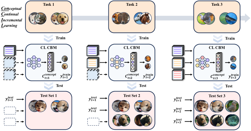
Figure 1: Schematic illustration of the Concept-Incremental and Class-Incremental Continual Learning (CICIL) task for CBMs. The figure depicts the sequential nature of the CICIL task, where each task $t$ introduces new classes and concepts. The training and testing datasets $\mathcal{D}_{t}^{\text{train}}$ and $\mathcal{D}_{t}^{\text{test}}$ for each task contain input feature vectors $\mathbf{x}$, concept vectors $\mathbf{c}$, and labels $y$. The cumulative concept set $\mathcal{C}^{\text{concept}}_{\leq t}$ expands over time, incorporating both previously learned and new concepts.

To date, no research has explored the integration of continual learning within CBM frameworks, especially in the context of concept-incremental and class-incremental tasks [10]. This is a significant gap, as real-world data is inherently dynamic, and any intelligent system must accommodate both the arrival of new classes and the evolution of concepts. The need for such integration can be clearly illustrated with real-world examples. Consider a medical diagnostic system using CBMs: as new diseases (classes) emerge and additional symptoms (concepts) are identified, the system must be able to learn from these new developments while retaining knowledge of previously learned diseases and symptoms. More importantly, new data will introduce new concepts, but it will also require the model to retain previously learned concepts, even if the classes associated with them do not persist across learning phases. This scenario involves both concept-incremental learning (where concepts accumulate over time) and class-incremental learning (where new classes emerge but are not accumulated across phases), forming a complex learning task that has not been addressed in the current CBM literature.

In this work, we define for the first time a concept-incremental and class-incremental continual learning task within the CBM framework, a novel challenge that closely mirrors real-world data collection and labeling practices. In this task, while new data at each phase introduces new classes, the concepts that the model must learn are cumulative—they expand and build upon concepts learned in previous phases. Crucially, new data contains both new concepts and a continuation of previously learned concepts, which the model must leverage to maintain its accuracy while adapting to evolving knowledge. This multi-phase, concept-incremental and class-incremental learning task is not only more aligned with real-world data but also poses significant challenges for existing CBM models that have not been designed to handle this kind of incremental learning.

Given the lack of solutions for this novel task, we propose the first continual learning framework for CBMs, specifically designed to address the unique challenges of concept-incremental and class-incremental learning. Our approach operates under realistic constraints: at each phase, only the current phase’s data and the model weights from the previous phase are available, reflecting the data privacy and storage limitations often found in real-world settings. Traditional approaches to continual learning either involve retraining the model on all historical data (which is computationally expensive and may violate privacy regulations) or fine-tuning on new data only [11] (which risks catastrophic forgetting [12]). In contrast, our framework leverages analytic learning principles [13] to reformulate the updates in the CBM’s concept and decision layers as a series of linear regression problems. This eliminates the need for gradient-based updates and effectively addresses catastrophic forgetting, ensuring that the model retains prior knowledge while adapting to new concepts and classes.

To achieve this, we introduce CONceptual Continual Incremental Learning (CONCIL), a framework that utilizes lightweight recursive matrix operations for model updates. This approach is computationally efficient and scalable, making it suitable for real-time applications and large-scale data processing. We prove theoretically that this method achieves "absolute knowledge memory," meaning the model behaves as though it had been trained on a centralized, comprehensive dataset, thus fully retaining the knowledge from previous phases. Through extensive empirical validation, we demonstrate that CONCIL outperforms traditional CBM methods in both concept-incremental and class-incremental settings.

The key contributions of this paper are as follows: (i) We define and address the concept-incremental and class-incremental continual learning task within the CBM framework, a novel challenge that reflects real-world data evolution. (ii) We propose a continual learning framework for CBMs that eliminates gradient-based updates and effectively retains prior knowledge without catastrophic forgetting. (iiii) We introduce CONCIL, a framework based on recursive matrix operations, which is computationally efficient and scalable for real-time and large-scale applications. (iv) We provide a comprehensive theoretical and empirical evaluation of the proposed framework, demonstrating its effectiveness in the context of continual learning tasks within CBMs.

2 Related Work

Concept Bottleneck Models (CBMs) are a class of XAI techniques that enhance model interpretability by using human-understandable concepts as intermediate representations within neural network architectures. CBMs encompass several variants that advance different aspects of interpretability and functionality. Original CBMs [14] aim to increase transparency by embedding concept-based layers within model architectures, while Interactive CBMs [15] improve predictive accuracy in interactive settings by selectively learning concepts. Further extensions, such as Post-hoc CBMs (PCBMs) [16] and Label-free CBMs [17], allow for the application of interpretability in pre-trained models and support unsupervised learning without explicit concept annotations. While these approaches contribute to interpretability, existing CBMs predominantly assume static datasets, limiting their applicability in real-world environments where data arrives in a continuous, dynamic stream with evolving concepts and classes. To address this critical limitation, our work is the first to define a continual learning paradigm specifically for CBMs, designed to handle scenarios that require both concept-incremental and class-incremental learning. This new paradigm enables CBMs to adapt to continuously evolving data environments, marking a significant departure from prior static data assumptions.

Class-Incremental Learning (CIL) has gained attention in recent years as a means to address catastrophic forgetting in models trained on incrementally arriving data [18, 19, 20]. CIL methods are typically divided into two main categories: replay-based and exemplar-free approaches. Replay-based methods, such as iCaRL [21] and ER [22], retain a subset of previously seen samples to replay during incremental training, thereby preserving prior knowledge. However, these methods often require storage of historical data, which can introduce privacy concerns and impose storage constraints. In contrast, exemplar-free approaches [19, 23, 24] aim to preserve prior knowledge through regularization or knowledge distillation without retaining past samples, though these methods often perform less effectively than replay-based methods. Both categories primarily rely on gradient-based updates, which can still lead to forgetting previously learned information when new data is introduced. Distinctly, our framework employs a gradient-free, analytic learning approach tailored to CBMs, effectively addressing catastrophic forgetting while ensuring computational efficiency.

While prior research has advanced interpretability in CBMs and mitigated forgetting in CIL, no existing work has combined these approaches to address the unique challenge of continual learning in CBMs. Our work uniquely defines the task of concept-incremental and class-incremental continual learning for CBMs and provides a tailored solution to address this task, filling a critical gap in XAI research. This approach enables CBMs to adapt to evolving data without sacrificing prior knowledge, establishing a new benchmark for interpretable models in dynamic environments.

3 Task Definition

We formally define the Concept-Incremental and Class-Incremental Continual Learning (CICIL) task for CBMs (See Figure 1). The learning process consists of $T$ sequential tasks, where each task $t\in{1,\dots,T}$ introduces new classes and contains both previously learned concepts and new concepts unique to the current task. For each task $t$, let $\mathcal{D}_{t}^{\text{train}}={(\mathbf{x}_{i},\mathbf{c}_{i},y_{i})}_{i=1}^{N_{t}}$ and $\mathcal{D}_{t}^{\text{test}}={(\mathbf{x}_{j},\mathbf{c}_{j},y_{j})}_{j=1}^{M_{t}}$ denote the training and testing datasets, respectively, where $\mathbf{x}_{i}\in\mathbb{R}^{d}$ represents the input feature vector, $\mathbf{c}_{i}\in\mathbb{R}^{L_{t}}$ is the concept vector, and $y_{i}\in\mathcal{C}_{t}$ is the label associated with task $t$. Here, $\mathcal{C}_{t}$ is the set of classes specific to task $t$, and the classes across tasks are disjoint, i.e., $\mathcal{C}_{t}\cap\mathcal{C}_{t^{\prime}}=\emptyset$ for $t^{\prime}\neq t$.

Each task $t$ involves a set of concepts $\mathcal{C}_{t}^{\text{concept}}={c^{1},\ldots,c^{L_{t}}}$, which includes a subset of previously learned concepts as well as new concepts unique to the current task. Consequently, at task $t$, the cumulative concept set is represented by $\mathcal{C}^{\text{concept}}_{\leq t}=\bigcup_{k=1}^{t}\mathcal{C}_{k}^{\text{concept}}$, ensuring that the model must learn and retain previously encountered concepts while integrating new ones. This setting requires CBMs not only to incrementally learn new classes in each task but also to expand their concept representations over time.

The CBM model in this setting consists of two primary components: (1) a concept extractor $g:\mathbb{R}^{d}\rightarrow\mathbb{R}^{L_{t}}$ that maps the input feature space to the concept space, and (2) a classifier $f:\mathbb{R}^{L_{\leq t}}\rightarrow\mathbb{R}$ that maps the accumulated concept space to the class label space for task $t$. For a given input $\mathbf{x}$, the predicted concept vector at task $t$ is given by $\hat{\mathbf{c}}=g(\mathbf{x})$, and the predicted label is $\hat{y}=f(g(\mathbf{x}))$.

Objective in Concept- and Class-Incremental Learning. At each task $t$, the objective is to learn parameters $\Theta_{t}={[\theta_{g},\theta_{f}]}$ for $[g,f]$, using both the new dataset $\mathcal{D}_{t}^{\text{train}}$ and the parameters from the previous task, $\Theta_{t-1}$. The updated model parameters $\Theta_{t}$ must satisfy two critical properties:

(i) Stability: The model must retain its ability to accurately predict concepts and classes learned in previous tasks ${1,\ldots,t-1}$, ensuring that accumulated knowledge is preserved and reducing the risk of catastrophic forgetting.

(ii) Plasticity: The model must adapt to new concepts and classes introduced in the current task $t$. This requires the concept extractor $g$ to recognize and represent new concepts while enabling the classifier $f$ to distinguish new classes without interference from prior learning.

The model is constrained to access only the current task’s data $\mathcal{D}_{t}^{\text{train}}$ and the parameters from the previous task $\Theta_{t-1}$, aligning with real-world scenarios where retaining all prior data may be impractical due to privacy or storage limitations.

The simultaneous increment of concepts and classes results in an increment of the output dimension for $\theta_{g}$ (this seems to be similar to common incremental continuous learning for classes), as well as an increment of both the input and output dimensions for $\theta_{f}$. This is a daunting task, so much so that we would argue that current deep learning approaches struggle to solve it. So we turned to machine learning for inspiration.

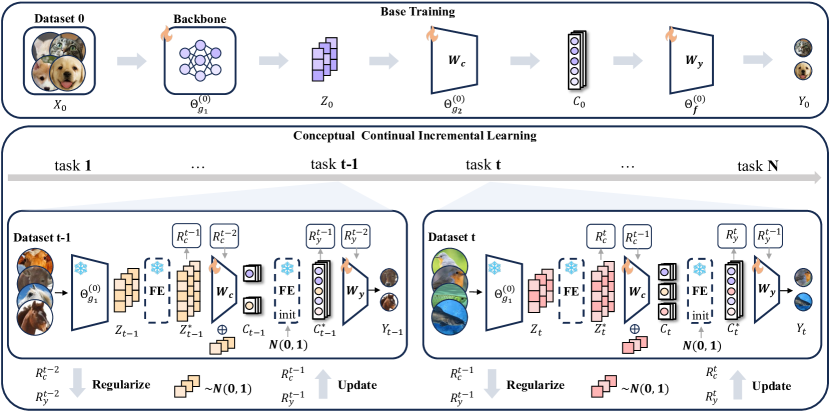
Figure 2: Schematic Overview of CONCIL Framework.

4 Method

This section details the proposed continual learning framework, CONceptual Continual Incremental Learning (CONCIL), designed for CBMs. CONCIL enables concept- and class-incremental learning through a recursive analytic approach, preserving historical knowledge without relying on prior data samples.

4.1 Model Architecture and Notation

Following the task definition, we extend the conventional CBM structure from $\mathbf{x}\to\mathbf{c}\to y$ to $\mathbf{x}\to\mathbf{z}\to\mathbf{c}\to y$, representing an intermediate feature representation $\mathbf{z}$ extracted by a backbone network. Formally:

$\mathbf{x}\in\mathbb{R}^{d}$ denotes the input data, $\mathbf{z}=g_{1}(\mathbf{x};\Theta_{g_{1}})\in\mathbb{R}^{d_{z}}$ represents the feature vector extracted by the backbone network $g_{1}$ with parameters $\Theta_{g_{1}}$, $\mathbf{c}=g_{2}(\mathbf{z};\Theta_{g_{2}})\in\mathbb{R}^{L_{t}}$ denotes the human-interpretable concept vector obtained via a concept mapping function $g_{2}$ with parameters $\Theta_{g_{2}}$, $y=f(\mathbf{c};\Theta_{f})\in\mathbb{R}^{y_{t}}$ is the final output predicted by a classifier $f$ with parameters $\Theta_{f}$.

At each learning phase $t$ in a continual learning scenario, the model receives a new dataset $\mathcal{D}_{t}=\{(\mathbf{x}_{i},\mathbf{c}_{i},y_{i})\}_{i=1}^{N_{t}}$, where previously unseen concepts and classes will appear. Over multiple phases, this incremental addition of knowledge requires the model to learn new information while retaining what was learned in earlier phases.

4.2 Base Training and Feature Expansion

In the initial training phase (base training), we train the backbone $g_{1}$, concept layer $g_{2}$, and classifier $f$ jointly on the first dataset $\mathcal{D}_{0}$ using standard backpropagation (BP). This produces initial parameter estimates $\Theta_{g_{1}}^{(0)}$, $\Theta_{g_{2}}^{(0)}$, and $\Theta_{f}^{(0)}$. For an input $\mathbf{x}$, the initial model output is:

$$y=f(g_{2}(\mathbf{z};\Theta_{g_{2}}^{(0)});\Theta_{f}^{(0)}),$$ (1)

where

$$\mathbf{z}=g_{1}(\mathbf{x};\Theta_{g_{1}}^{(0)}).$$ (2)

After this phase, the backbone parameters $\Theta_{g_{1}}^{(0)}$ are frozen as $\Theta_{g_{1}}$. To enhance the feature space, we introduce a Feature Expansion (FE) transformation that maps the extracted feature $\mathbf{z}$ to a higher-dimensional space $\mathbf{z}^{*}$. This expanded bfeature representation $\mathbf{z}^{*}$ facilitates analytic learning by enlarging the parameter space, essential for robust concept separation in subsequent phases.

The expanded feature $\mathbf{z}^{*}$ is defined as:

$$\mathbf{z}^{*}=\phi(\mathbf{z};W_{fe})=\sigma(\mathbf{z}W_{fe}),$$ (3)

where $W_{fe}\in\mathbb{R}^{d_{z}\times d_{z^{*}}}$ is the expansion matrix initialized with values from a normal distribution, and $\sigma$ is a nonlinear activation function ReLU.

4.3 Non-Recursive Solution for Concept-Incremental Learning

With the expanded feature representation $\mathbf{z}^{*}$, we formulate the concept mapping problem as a linear regression from $\mathbf{z}^{*}$ to $\mathbf{c}$ using a closed-form analytic solution. For each phase $t$, the objective is to learn a mapping matrix $W_{c}^{(t)}\in\mathbb{R}^{d_{z^{*}}\times d_{L_{t}}}$ that minimizes the following regularized loss:

$$\arg\min_{W_{c}^{(t)}}\|C_{t}-Z^{*}_{t}W_{c}^{(t)}\|_{F}^{2}+\lambda_{1}\|W_{c}^{(t)}\|_{F}^{2},$$ (4)

where $C_{t}\in\mathbb{R}^{N_{t}\times d_{L_{t}}}$ is the matrix of concept labels in phase $t$, $Z^{*}_{t}\in\mathbb{R}^{N_{t}\times d_{{z}^{*}}}$ is the expanded feature matrix at phase $t$, and $\lambda_{1}$ is a regularization parameter. This formulation leads to the closed-form solution:

$$\hat{W}_{c}^{(t)}=({Z^{*}}_{t}^{T}{Z^{*}}_{t}+\lambda_{1}I)^{-1}{Z^{*}}_{t}^{T}C_{t}.$$ (5)

4.4 Feature Expansion after Concept Mapping

We define the concept of network prediction in this phase as $\hat{C_{t}}=Z^{*}_{t}W_{c}^{(t)}\in\mathbb{R}^{N_{t}\times L_{t}}$. To enhance the concept space, we introduce a Feature Expansion (FE) transformation that maps the extracted feature $\hat{C_{t}}\in\mathbb{R}^{N_{t}\times\mathbb{R}^{d_{\hat{C_{t}}^{*}}}}$ to a higher-dimensional space $\hat{C_{t}^{*}}$, too. This expanded concept space representation $\hat{C_{t}^{*}}$ facilitates analytic learning by enlarging the parameter space.

The expanded concept $\hat{C_{t}}^{*}$ is defined as:

$$\hat{C_{t}^{*}}=\phi(\hat{C_{t}};W_{fe}^{\prime})=\sigma(\hat{C_{t}}W_{fe}^{\prime}),$$ (6)

where $W_{fe}^{\prime}\in\mathbb{R}^{d_{L_{t}}}\times\mathbb{R}^{d_{\hat{C_{t}}^{*}}}$ is the expansion matrix initialized with values from a normal distribution, and $\sigma$ is a nonlinear activation function ReLU. It is important to emphasize that the weights of the initialization here change (incrementally) both the input dimension and the output dimension in each phase, due to the increment of the concept space before unexpanded.

4.5 Non-Recursive Solution for Class-Incremental Learning

With the expanded concept representation $\hat{C_{t}^{*}}$, we formulate the concept mapping problem as a linear regression from $\hat{C_{t}^{*}}$ to $\mathbf{y}$ using a closed-form analytic solution, too. For each phase $t$, the objective is to learn a mapping matrix $W_{y}^{(t)}\in\mathbb{R}^{d_{\hat{C_{t}^{*}}}\times d_{y_{t}}}$ that minimizes the following regularized loss:

$$\arg\min_{W_{y}^{(t)}}\|Y_{t}-\hat{C_{t}^{*}}W_{y}^{(t)}\|_{F}^{2}+\lambda_{2}\|W_{y}^{(t)}\|_{F}^{2},$$ (7)

where $Y_{t}\in\mathbb{R}^{N_{t}\times d_{y_{t}}}$ is the matrix of concept labels in phase $t$, $\hat{C_{t}^{*}}\in\mathbb{R}^{N_{t}\times d_{\hat{C_{t}^{*}}}}$ is the expanded concept matrix at phase $t$, and $\lambda_{2}$ is a regularization parameter. This formulation leads to the closed-form solution:

$$\hat{W}_{y}^{(t)}=(\hat{C_{t}^{*}}^{T}\hat{C_{t}^{*}}+\lambda_{2}I)^{-1}\hat{C_{t}^{*}}^{T}Y_{t}.$$ (8)

4.6 Conversion to Recursive Form

To make this solution efficient in a continual learning setting, we convert the non-recursive formulation into a recursive update form. This recursive transformation allows the model to update parameters incrementally with only the current phase’s data, eliminating the need to retain all prior data.

Let $\mathbf{R_{c}}^{(t)}=\left(\sum_{i=0}^{t}{Z}_{i}^{*T}{Z^{*}}_{i}+\lambda_{1}I\right)^{-1}$ denote the regularized inverse correlation matrix for concept mapping at phase $t$. Using the matrix inversion lemma (Woodbury formula), we derive the recursive update for $\mathbf{R_{c}}^{(t)}$. The matrix inversion lemma states that for invertible matrices $A_{c}\in\mathbb{R}^{d_{A_{c}}\times d_{A_{c}}}$, $U_{c}\in\mathbb{R}^{d_{A_{c}}\times d_{U_{c}}}$, $C_{c}\in\mathbb{R}^{d_{U_{c}}\times d_{C_{c}}}$, and $V_{c}\in\mathbb{R}^{d_{C_{c}}\times d_{A_{c}}}$, we have:

$$(A_{c}+U_{c}C_{c}V_{c})^{-1}=A_{c}^{-1}-A_{c}^{-1}U_{c}(C_{c}^{-1}+V_{c}A_{c}^{-1}U_{c})^{-1}V_{c}A_{c}^{-1}.$$ (9)

In our context, we set $A_{c}=\sum_{i=0}^{t-1}{Z^{*}}_{i}^{T}Z^{*}_{i}+\lambda_{1}I$. Thus, we can express the recursive form as:

$$\mathbf{R_{c}}^{(t)}=\left(\sum_{i=0}^{t}{Z^{*}}_{i}^{T}Z^{*}_{i}+\lambda_{1}I\right)^{-1}=\mathbf{R_{c}}^{(t-1)}-\mathbf{R_{c}}^{(t-1)}{Z}_{t}^{*T}\left(I+{Z}^{*}_{t}\mathbf{R_{c}}^{(t-1)}{Z}_{t}^{*T}\right)^{-1}{Z}_{t}^{*}\mathbf{R_{c}}^{(t-1)}.$$ (10)

Similarly, for $\mathbf{R_{y}}^{(t)}=\left(\sum_{i=0}^{t}\hat{C_{t}^{*}}^{T}\hat{C_{t}^{*}}+\lambda_{2}I\right)^{-1}$ which denote the regularized inverse correlation matrix for class mapping at phase $t$, we alse can express the recursive form as:

$$\mathbf{R_{y}}^{(t)}=\left(\sum_{i=0}^{t}\hat{C_{t}^{*}}^{T}\hat{C_{t}^{*}}+\lambda_{2}I\right)^{-1}=\mathbf{R_{y}}^{(t-1)}-\mathbf{R_{y}}^{(t-1)}\hat{C_{t}^{*}}^{T}\left(I+\hat{C_{t}^{*}}\mathbf{R_{y}}^{(t-1)}\hat{C_{t}^{*}}^{T}\right)^{-1}\hat{C_{t}^{*}}\mathbf{R_{y}}^{(t-1)}.$$ (11)

This derivation provides an efficient method for updating the inverse correlation matrix, allowing us to utilize the current phase data without recalculating the entire cumulative sum. For the detailed theoretical derivation of this recursive update, please refer to Appendix A.

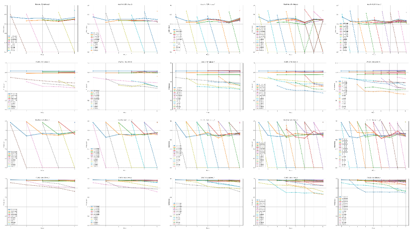
Figure 3: Visualization of Concept and Class Accuracy Across Phases for Baseline and CONCIL. The first and third rows show the results for the Baseline model on the CUB and AwA datasets, respectively. The second and fourth rows display the results for the CONCIL model on the CUB and AwA datasets, respectively. Each column represents a phase setting.

4.7 Recursive Update for Weights

Similarly, we can express the recursive update for the concept layer and classifier weights $W_{c}^{(t)}$ and $W_{y}^{(t)}$ in terms of the previous phase’s weights $W_{c}^{(t-1)}$ and $W_{y}^{(t-1)}$ and the current phase data. Given the recursive form of $\mathbf{R_{c}}^{(t)}$ and $\mathbf{R_{y}}^{(t)}$, the concept layer weight update can be formulated as:

$$W_{c}^{(t)}=\left[W_{c}^{(t-1)}-\mathbf{R_{c}}^{(t)}{Z^{*}}_{t}^{T}{Z^{*}}_{t}W_{c}^{(t-1)}\quad\mathbf{R_{c}}^{(t)}{Z^{*}}_{t}^{T}C_{t}\right],$$ (12)

and the classifier weight update can be formulated as:

$$W_{y}^{(t)}=\left[W_{y}^{(t-1)}-\mathbf{R_{y}}^{(t)}\hat{C_{t}^{*}}^{T}\hat{C_{t}^{*}}W_{y}^{(t-1)}\quad\mathbf{R_{y}}^{(t)}\hat{C_{t}^{*}}^{T}Y_{t}\right],$$ (13)

This recursive form ensures that the concept layer weights $W_{c}^{(t)}$ and classifier weights $W_{y}^{(t)}$ at phase $t$ incorporate information from both the current phase data $({{Z^{*}}_{t}}^{T},{C_{t}}^{T})$, ${(\hat{C_{t}^{*}}}^{T},{Y_{t}}^{T})$ and the accumulated knowledge from all previous phases.

4.8 Properties of the Recursive Framework

The recursive update framework provides several key advantages:

(i) Absolute Knowledge Retention: By maintaining the recursive update form, the model preserves prior knowledge without requiring access to historical data, achieving results equivalent to joint training across all phases.

(ii) Privacy Protection: Since the recursive update relies only on the current phase data and the correlation matrix $\mathbf{R_{c}},\mathbf{R_{y}}$, it does not require storage of previous phase data, inherently preserving data privacy.

(iii) Computational Efficiency: The recursive framework significantly reduces the computational load by avoiding redundant recalculations, making it suitable for real-time continual learning scenarios.

5 Experiments and Results

5.1 Datasets and Backbone

This section outlines the datasets and the backbone architecture employed in our experiments. Our study focuses on evaluating the effectiveness of our proposed method on two well-known benchmark datasets: the Caltech-UCSD Birds-200-2011 (CUB) [25] and the Animals with Attributes (AwA) [26] datasets.

CUB Dataset. The Caltech-UCSD Birds-200-2011 (CUB) dataset [25] is tailored for the task of bird classification, featuring 11,788 images representing 200 distinct species. Accompanying these images are 312 binary attributes, which provide rich, high-level semantic descriptions of the birds.

AwA Dataset. The AwA dataset consists of 37,322 images from 50 animal categories, each annotated with 85 binary attributes. We divided the dataset into training and testing sets, with an equal distribution of images per class, resulting in 18,652 training images and 18,670 testing images. No modifications were made to the binary attributes, preserving the original annotations for both training and evaluation.

Backbone Architecture. To serve as the foundation for our experiments, we utilized a pre-trained ResNet50 model as the backbone.

5.2 Setting

To evaluate the performance of our proposed Concept-Incremental and Class-Incremental Continual Learning (CICIL) task framework, we designed a series of experiments on the CUB and AwA datasets, adapting them to fit the concept-incremental and class-incremental continual learning paradigm. The experimental setup is structured into multiple phases, each corresponding to a learning task with a progressively increasing number of classes and concepts.

Phase-wise Data Splitting and Access Control. For both the CUB and AwA datasets, the initial phase (Phase 1) is defined such that only the first $n\%$ of the total classes and the first $m\%$ of the concepts associated with these classes are accessible for training. Specifically, in Phase 1, the model is trained on a subset of the data, which includes the earliest $n\%$ of the classes and the corresponding $m\%$ of the concepts. This initial setup allows the model to establish a baseline understanding of the problem domain before being exposed to new information.

Subsequent phases are designed to incrementally introduce new classes and concepts. From Phase 2 onwards, each phase incorporates an additional $\frac{1-n\%}{p-1}$ of the remaining classes and an additional $\frac{1-m\%}{p-1}$ of the concepts, where $p$ denotes the total number of phases. This gradual increase ensures that the model is challenged with learning new information while maintaining the stability of previously acquired knowledge. It is important to note that for each phase, the model has access only to the current phase’s data and the parameters from the immediately preceding phase, simulating realistic constraints where storing and revisiting all past data might not be feasible due to practical considerations such as privacy and storage limitations.

In our experiments, we set $n=50$, $m=50$, and $p=[2,3,4,5,6,7,8,9]$.

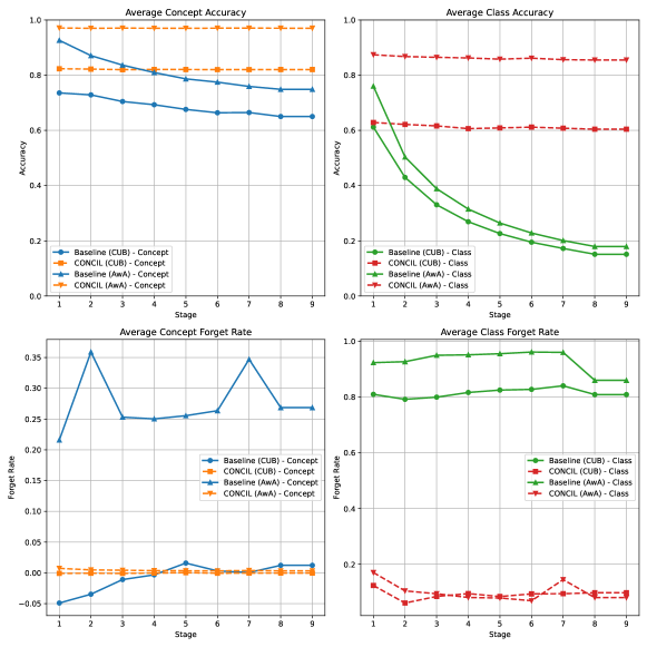
Figure 4: Performance Comparison of Baseline and CONCIL Models on CUB and AwA Datasets. The first row shows the average concept accuracy (left) and average class accuracy (right) for the Baseline and CONCIL models on the CUB and AwA datasets. The second row displays the average concept forget rate (left) and average class forget rate (right) for both models on the same datasets. Each plot visualizes the metrics across different phases, highlighting the superior performance and lower forgetting rates of the CONCIL model compared to the Baseline model.

Table 1: Comparison of Model Performance Across Phases: Concept and Class Accuracy, and Average Forgetting Rates for CUB and AwA Datasets. Higher accuracy and lower forgetting rates indicate better performance.

Metric Phase 2 Phase 3 Phase 4 Phase 5 Phase 6 Phase 7 Phase 8 Phase 9 Average Average Concept Accuracy $\uparrow$ (CUB) Baseline 0.7357 0.7286 0.7046 0.6930 0.6760 0.6638 0.6647 0.6502 0.6896 CONCIL 0.8233 0.8220 0.8200 0.8207 0.8205 0.8202 0.8203 0.8204 0.8209 Average Class Accuracy $\uparrow$ (CUB) Baseline 0.6119 0.4297 0.3305 0.2692 0.2263 0.1950 0.1723 0.1513 0.2983 CONCIL 0.6287 0.6216 0.6163 0.6064 0.6090 0.6118 0.6079 0.6043 0.6133 Average Concept Accuracy $\uparrow$ (AwA) Baseline 0.9262 0.8709 0.8364 0.8095 0.7866 0.7747 0.7592 0.7488 0.8140 CONCIL 0.9708 0.9699 0.9704 0.9701 0.9699 0.9703 0.9704 0.9702 0.9703 Average Class Accuracy $\uparrow$ (AwA) Baseline 0.7601 0.5036 0.3888 0.3149 0.2644 0.2283 0.2010 0.1794 0.3550 CONCIL 0.8739 0.8675 0.8647 0.8624 0.8580 0.8616 0.8561 0.8550 0.8624 Average Concept Forget Rate $\downarrow$ (CUB) Baseline -0.0490 -0.0347 -0.0109 -0.0032 0.0159 0.0032 0.0006 0.0122 -0.0082 CONCIL -0.0008 -0.0006 -0.0008 -0.0003 0.0003 -0.0006 -0.0003 -0.0004 -0.0004 Average Class Forget Rate $\downarrow$ (CUB) Baseline 0.8101 0.7922 0.8000 0.8168 0.8254 0.8279 0.8407 0.8093 0.8153 CONCIL 0.1239 0.0610 0.0847 0.0948 0.0843 0.0938 0.0945 0.0978 0.0919 Average Concept Forget Rate $\downarrow$ (AwA) Baseline 0.2158 0.3588 0.2530 0.2502 0.2554 0.2635 0.3470 0.2685 0.2765 CONCIL 0.0073 0.0048 0.0043 0.0036 0.0034 0.0032 0.0038 0.0033 0.0042 Average Class Forget Rate $\downarrow$ (AwA) Baseline 0.9239 0.9273 0.9503 0.9519 0.9559 0.9619 0.9607 0.8603 0.9365 CONCIL 0.1704 0.1045 0.0943 0.0808 0.0791 0.0692 0.1449 0.0803 0.1029

5.3 Metrics

To comprehensively evaluate the performance of our CICIL task framework, we propose four key metrics that measure both the accuracy and the stability of the model across different phases. The Average Concept Accuracy ($A_{\text{concept}}(t)$) and Average Class Accuracy ($A_{\text{class}}(t)$) measure the mean accuracy of concept and class predictions, respectively, across all tasks up to the current phase $t$:

$$A_{\text{concept}}(t)=\frac{1}{t}\sum_{k=1}^{t}\text{Accuracy}(\mathcal{D}_{k}^{\text{test}},\mathbf{c}),$$ (14)

$$A_{\text{class}}(t)=\frac{1}{t}\sum_{k=1}^{t}\text{Accuracy}(\mathcal{D}_{k}^{\text{test}},y).$$ (15)

The Average Concept Forgetting Rate ($F_{\text{concept}}(t)$) and Average Class Forgetting Rate ($F_{\text{class}}(t)$) measure the mean rate at which the model forgets previously learned concepts and classes, respectively, across all tasks up to the current phase $t$:

$$F_{\text{concept}}(t)=\frac{1}{t-1}\sum_{k=1}^{t-1}\left(\max_{1\leq j<t}\text{Accuracy}(\mathcal{D}_{k}^{\text{test}},\mathbf{c})-\text{Accuracy}(\mathcal{D}_{k}^{\text{test}},\mathbf{c})_{t}\right),$$ (16)

$$F_{\text{class}}(t)=\frac{1}{t-1}\sum_{k=1}^{t-1}\left(\max_{1\leq j<t}\text{Accuracy}(\mathcal{D}_{k}^{\text{test}},y)-\text{Accuracy}(\mathcal{D}_{k}^{\text{test}},y)_{t}\right).$$ (17)

These metrics provide a balanced evaluation of the model’s ability to learn new information while retaining previously acquired knowledge.

5.4 Setup

We configured the experimental setup with the following parameters and techniques. We set $\lambda_{1}=500$ , $\lambda_{2}=1$, $d_{{z}^{*}}=25000$, and $d_{\hat{C_{t}}^{*}}=25000$. The initial learning rate was set to $1\times 10^{-4}$, and a weight decay of $5\times 10^{-5}$ was applied to prevent overfitting. An exponential learning rate scheduler with a decay factor ($\gamma$) of 0.95 was used to enhance the model’s generalization ability. The concept loss, crucial for aligning learned features with human-interpretable concepts, was weighted by a factor of 0.5 to balance the primary task loss. During the baseline training phase and each phase of the CICIL task framework, the datasets were augmented with random color jittering, random horizontal flipping, and random cropping to a resolution of 256 pixels, following the guidelines established by Koh et al. [14] with minor adjustments to the resolution. For inference, images were center-cropped and resized to 256 pixels to ensure consistency with the training input size. Each phase of the CICIL task framework was trained for a single epoch, reflecting the nature of the task as a linear fitting problem, while the baseline model was trained for 50 epochs per phase, consistent with the original CBM setup. All experiments were conducted on an A800 GPU to provide the necessary computational power for efficient processing.

5.5 Experimental Results and Analysis

The results presented in Table 1 clearly demonstrate the superiority of our proposed method, CONCIL, over the baseline model on both the CUB and AwA datasets. Specifically, for average concept accuracy, CONCIL outperforms the baseline by 19% on the CUB dataset and 19.2% on the AwA dataset. This consistent improvement across different datasets underscores the robustness and generalizability of CONCIL.

For average class accuracy, the performance gap is even more pronounced. On the CUB dataset, CONCIL achieves an improvement of 31.5% points over the baseline, while on the AwA dataset, this improvement is even more significant at 50.7% points. These substantial gains in class accuracy highlight the effectiveness of CONCIL in handling complex classification tasks.

Moreover, CONCIL significantly reduces the forgetting rate, a critical metric in continual learning. The average class forgetting rate decreases by 88.7% on the CUB dataset and 89% on the AwA dataset. This remarkable reduction in forgetting rate indicates that CONCIL not only excels in learning new concepts but also effectively retains previously learned information, thereby addressing one of the primary challenges in continual learning.

To gain a more intuitive understanding of these performance differences, Figure 4 provides a visual comparison of the baseline and CONCIL models. As the number of training steps increases, the average accuracy of the baseline model drops significantly, while the average forgetting rate gradually increases. This trend is particularly evident in the later phases of training, where the baseline model’s performance deteriorates markedly.

In contrast, the CONCIL model maintains a relatively stable level of performance throughout the training process. It consistently achieves higher average accuracy and exhibits a much lower forgetting rate compared to the baseline. This stability and consistency in performance across different phases highlight the superior capabilities of CONCIL in managing the trade-off between learning new tasks and retaining old knowledge.

Furthermore, the visualizations in Figure 3 offer additional insights into the performance dynamics of both models across different phases. It is evident that CONCIL consistently outperforms the baseline in both concept and class accuracy, maintaining high levels of performance even as the complexity of the tasks increases.

6 Conclusion

In conclusion, the introduction of CONceptual Continual Incremental Learning (CONCIL) marks a significant step and the first step forward in the field of Continual Learning for Concept Bottleneck Models (CBMs). By reformulating concept and decision layer updates as linear regression problems, CONCIL not only mitigates the risk of catastrophic forgetting but also offers a computationally efficient solution suitable for real-time and large-scale data applications. The experimental results validate the effectiveness of CONCIL in achieving "absolute knowledge memory" and outperforming traditional CBM methods in both concept- and class-incremental settings. This work sets a new benchmark for continual learning in CBMs, paving the way for more adaptive and interpretable AI systems capable of handling the dynamic nature of real-world data. However, future research should focus on enhancing the model’s ability to manage non-linear relationships, improving its robustness to sudden changes in data distribution, and optimizing computational efficiency for even larger-scale applications.

Appendix A Theoretical Derivation of Recursive Update

In this appendix, we detail the theoretical derivation of the recursive update for the regularized inverse correlation matrix $\mathbf{R_{c}}^{(t)}$.

The matrix inversion lemma (Woodbury formula) provides the foundation for transforming the non-recursive solution into a recursive one. It states that for any invertible matrix $A_{c}$, and matrices $U_{c}$, $C_{c}$, and $V_{c}$ as defined above, we have:

$$(A_{c}+U_{c}C_{c}V_{c})^{-1}=A_{c}^{-1}-A_{c}^{-1}U_{c}(C_{c}^{-1}+V_{c}A_{c}^{-1}U_{c})^{-1}V_{c}A_{c}^{-1}.$$ (18)

Applying this to our problem, we let:

$$A_{c}=\sum_{i=0}^{t-1}{Z^{*}}_{i}^{T}{Z^{*}}_{i}+\lambda_{1}I,$$ (19)

which leads to:

$$\mathbf{R_{c}}^{(t)}=(A_{c}+{Z^{*}}_{t}{Z^{*}}_{t}^{T})^{-1}.$$ (20)

By applying the lemma, we find:

$$\mathbf{R_{c}}^{(t)}=A_{c}^{-1}-A_{c}^{-1}{Z^{*}}_{t}(I+{Z^{*}}_{t}^{T}A_{c}^{-1}{Z^{*}}_{t})^{-1}{Z^{*}}_{t}^{T}A_{c}^{-1}.$$ (21)

Recognizing $A_{c}^{-1}$ as $\mathbf{R_{c}}^{(t-1)}$, we can derive the recursive form:

$$\mathbf{R_{c}}^{(t)}=\mathbf{R_{c}}^{(t-1)}-\mathbf{R_{c}}^{(t-1)}{Z^{*}}_{t}^{T}(I+{Z^{*}}_{t}\mathbf{R_{c}}^{(t-1)}{Z^{*}}_{t}^{T})^{-1}{Z^{*}}_{t}\mathbf{R_{c}}^{(t-1)}.$$ (22)

This shows how to update the correlation matrix recursively based solely on the current phase data, thus maintaining computational efficiency while ensuring absolute knowledge retention.

References

- [1] Yann LeCun, Yoshua Bengio, and Geoffrey Hinton. Deep learning. Nature, 521(7553):436–444, May 2015.
- [2] Wojciech Samek, Gregoire Montavon, Sebastian Lapuschkin, Christopher J. Anders, and Klaus-Robert Muller. Explaining deep neural networks and beyond: A review of methods and applications. Proceedings of the IEEE, 109(3):247–278, March 2021.
- [3] Zhenge Zhao, Panpan Xu, Carlos Scheidegger, and Liu Ren. Human-in-the-loop extraction of interpretable concepts in deep learning models. IEEE Transactions on Visualization and Computer Graphics, 28(1):780–790, 2022.
- [4] Luca Longo, Mario Brcic, Federico Cabitza, Jaesik Choi, Roberto Confalonieri, Javier Del Ser, Riccardo Guidotti, Yoichi Hayashi, Francisco Herrera, Andreas Holzinger, Richard Jiang, Hassan Khosravi, Freddy Lecue, Gianclaudio Malgieri, Andrés Páez, Wojciech Samek, Johannes Schneider, Timo Speith, and Simone Stumpf. Explainable artificial intelligence (xai) 2.0: A manifesto of open challenges and interdisciplinary research directions. Information Fusion, 106:102301, June 2024.
- [5] Tongtong Wu, Linhao Luo, Yuan-Fang Li, Shirui Pan, Thuy-Trang Vu, and Gholamreza Haffari. Continual learning for large language models: A survey, 2024.
- [6] Liyuan Wang, Xingxing Zhang, Hang Su, and Jun Zhu. A comprehensive survey of continual learning: Theory, method and application, 2024.
- [7] Michael McCloskey and Neal J. Cohen. Catastrophic interference in connectionist networks: The sequential learning problem. volume 24 of Psychology of Learning and Motivation, pages 109–165. Academic Press, 1989.
- [8] James L. McClelland, Bruce L. McNaughton, and Randall C. O’Reilly. Why there are complementary learning systems in the hippocampus and neocortex: insights from the successes and failures of connectionist models of learning and memory. Psychological review, 102 3:419–457, 1995.
- [9] James Kirkpatrick, Razvan Pascanu, Neil Rabinowitz, Joel Veness, Guillaume Desjardins, Andrei A. Rusu, Kieran Milan, John Quan, Tiago Ramalho, Agnieszka Grabska-Barwinska, Demis Hassabis, Claudia Clopath, Dharshan Kumaran, and Raia Hadsell. Overcoming catastrophic forgetting in neural networks. Proceedings of the National Academy of Sciences, 114(13):3521–3526, March 2017.
- [10] Gido M. van de Ven, Tinne Tuytelaars, and Andreas S. Tolias. Three types of incremental learning. Nature Machine Intelligence, 4(12):1185–1197, December 2022.
- [11] Yong Lin, Hangyu Lin, Wei Xiong, Shizhe Diao, Jianmeng Liu, Jipeng Zhang, Rui Pan, Haoxiang Wang, Wenbin Hu, Hanning Zhang, Hanze Dong, Renjie Pi, Han Zhao, Nan Jiang, Heng Ji, Yuan Yao, and Tong Zhang. Mitigating the alignment tax of rlhf, 2024.
- [12] Yun Luo, Zhen Yang, Fandong Meng, Yafu Li, Jie Zhou, and Yue Zhang. An empirical study of catastrophic forgetting in large language models during continual fine-tuning, 2024.
- [13] Aytac Gogus. Analytic Learning, pages 237–241. Springer US, Boston, MA, 2012.
- [14] Pang Wei Koh, Thao Nguyen, Yew Siang Tang, Stephen Mussmann, Emma Pierson, Been Kim, and Percy Liang. Concept bottleneck models. In International conference on machine learning, pages 5338–5348. PMLR, 2020.
- [15] Kushal Chauhan, Rishabh Tiwari, Jan Freyberg, Pradeep Shenoy, and Krishnamurthy Dvijotham. Interactive concept bottleneck models. In Proceedings of the AAAI Conference on Artificial Intelligence, volume 37, pages 5948–5955, 2023.
- [16] Mert Yuksekgonul, Maggie Wang, and James Zou. Post-hoc concept bottleneck models. arXiv preprint arXiv:2205.15480, 2022.
- [17] Tuomas Oikarinen, Subhro Das, Lam M Nguyen, and Tsui-Wei Weng. Label-free concept bottleneck models. arXiv preprint arXiv:2304.06129, 2023.
- [18] Liyuan Wang, Xingxing Zhang, Hang Su, and Jun Zhu. A comprehensive survey of continual learning: Theory, method and application. IEEE Transactions on Pattern Analysis and Machine Intelligence, 46(8):5362–5383, 2024.
- [19] Zhizhong Li and Derek Hoiem. Learning without forgetting. IEEE transactions on pattern analysis and machine intelligence, 40(12):2935–2947, 2017.
- [20] Young D Kwon, Jagmohan Chauhan, and Cecilia Mascolo. Fasticarl: Fast incremental classifier and representation learning with efficient budget allocation in audio sensing applications. arXiv preprint arXiv:2106.07268, 2021.
- [21] Sylvestre-Alvise Rebuffi, Alexander Kolesnikov, Georg Sperl, and Christoph H Lampert. icarl: Incremental classifier and representation learning. In Proceedings of the IEEE conference on Computer Vision and Pattern Recognition, pages 2001–2010, 2017.
- [22] David Rolnick, Arun Ahuja, Jonathan Schwarz, Timothy Lillicrap, and Gregory Wayne. Experience replay for continual learning. Advances in neural information processing systems, 32, 2019.
- [23] Rahaf Aljundi, Francesca Babiloni, Mohamed Elhoseiny, Marcus Rohrbach, and Tinne Tuytelaars. Memory aware synapses: Learning what (not) to forget. In Proceedings of the European conference on computer vision (ECCV), pages 139–154, 2018.
- [24] Zhongzheng Qiao, Minghui Hu, Xudong Jiang, Ponnuthurai Nagaratnam Suganthan, and Ramasamy Savitha. Class-incremental learning on multivariate time series via shape-aligned temporal distillation. In ICASSP 2023-2023 IEEE International Conference on Acoustics, Speech and Signal Processing (ICASSP), pages 1–5. IEEE, 2023.
- [25] Catherine Wah, Steve Branson, Peter Welinder, Pietro Perona, and Serge Belongie. The caltech-ucsd birds-200-2011 dataset. 2011.
- [26] Yongqin Xian, Christoph H Lampert, Bernt Schiele, and Zeynep Akata. Zero-shot learning—a comprehensive evaluation of the good, the bad and the ugly. IEEE transactions on pattern analysis and machine intelligence, 41(9):2251–2265, 2018.