On turbulence for spacetimes with stable trapping

Abstract

Motivated by understanding the nonlinear gravitational dynamics of spacetimes admitting stably trapped null geodesics, such as ultracompact objects and black string solutions to general relativity, we explore the dynamics of nonlinear scalar waves on a simple (fixed) model geometry with stable trapping. More specifically, we consider the time evolution of solutions to the cubic (defocusing) wave equation on a four-dimensional static, spherically symmetric, and asymptotically flat (horizonless) spacetime admitting a stable photon sphere.

Unlike the known results for scalar waves on spacetimes with unstable trapping, our study shows fundamental differences between linear and nonlinear scalar dynamics. The local energy, as well as all local higher-order energies, of solutions to the linear wave equation on our model spacetime can be rigorously proven to remain uniformly bounded and to decay uniformly in time. However, due to the presence of stable trapping, the uniform decay rate is slow. To help elucidate how the slow linear decay affects solutions to the nonlinear wave equation considered, we examine numerical solutions of the latter, restricting to axisymmetric initial data in this work. In contrast to the linear dynamics, we exhibit a family of nonlinear solutions with turbulent behaviour. Within the region of stable trapping, the slow linear decay allows local higher-order energies of the nonlinear solution to grow over the time interval that we numerically evolve. The growth is induced by a direct energy cascade: Beginning with initial data containing a small number of low-order multipole modes, a spectrum of high-order multipole modes are populated in time by the nonlinear interactions and eventually dominate over the low-modes in the evolution.

That the system exhibits a direct cascade limits the time over which our numerical scheme can provide convergent solutions for the short-wavelength structure that develops, and hence we can only speculate what this intermediate-time dynamics implies for the nonlinear stability of the motivating spacetimes in general relativity. Nevertheless, we provide a heuristic argument suggesting that, if a similar behaviour occurs for gravitational wave perturbations of these spacetimes, it would likely not generically lead to black hole or singularity formation.

I Introduction

The dynamics of nonlinear waves is a classical theme in the mathematical study of partial differential equations. From the physical perspective, nonlinear wave equations describe a vast and diverse range of phenomena [1], whose domains include fluid dynamics, continuum mechanics, elasticity theory, nonlinear optics, and plasma physics, and often serve as models for more complicated physical systems. In the present paper, we consider nonlinear waves on a fixed, curved spacetime geometry as a model for the gravitational wave dynamics of certain classes of solutions to the Einstein equations. The latter are notoriously challenging to analyse, both rigorously and numerically, and there is a long history of attempting to gain insights into their putative dynamics using simpler nonlinear wave models.

The motivating spacetimes for this work are ultracompact objects in four-dimensional, asymptotically flat spacetimes and higher-dimensional black hole spacetimes with a compact extra-dimension known as black strings. By an ultracompact object, we refer to any linearly stable, horizonless soliton or star-like solution to the relevant non-vacuum Einstein equations that is sufficiently compact to possess a region of stably trapped null geodesics. In spherical symmetry, this requires the surface of the star (or the majority of its energy, if it does not have a well-defined surface) to be within an areal radius of $\sim 3M$, with $M$ being the ADM mass of the spacetime. Such compact objects need to be composed of “exotic” matter (ordinary matter at nuclear densities, as occurs in neutron stars, does not suffice), hypothetical examples of which include certain kinds of boson stars [2, 3], black shells [4], fuzzballs [5], or gravastars [6] (see [7] for a review with a comprehensive list of candidates, and current observational constraints on their existence). Black strings and their geometry will be described in Section I.4, where their relation to the present work is also discussed. As with ultracompact objects, black strings possess a region of stably trapped null geodesics [8, 9], including those black strings with sufficiently small compact extra-dimension so as to be free of the long-wavelength Gregory–Laflamme instability [10].

The presence of stable null geodesic trapping is key to the physics of nonlinear gravitational wave perturbations of these spacetimes. Such physics is what the nonlinear scalar waves considered in the present paper aim to model.

In the following Sections I.1 and I.2, we describe some aspects of the dynamics of both linear and nonlinear waves in the presence of null geodesic trapping. These sections provide the relevant context for the numerical results presented in this paper, which are outlined in Section I.3. In Section I.4, we elaborate on the motivation for the present work in connection to the dynamics of black strings. Section I.5 concludes the introduction and provides an outline of the bulk of the paper.

I.1 Linear waves in the presence of trapping

The dynamics of scalar waves is very informative, already at the linear level, of the interaction between the geometry of a spacetime and the dispersion of its perturbations. In particular, geometric properties of null geodesics of the spacetime, such as the possible presence of trapped null geodesics, play a key role.

Provided that solutions to the linear wave equation

$$\Box_{g}\phi=0$$ (1)

can be shown to decay uniformly in time on a given (fixed) stationary spacetime, if trapped null geodesics are present, then the uniform decay rate may crucially depend on the nature of trapping. Unstable trapping is more favorable for dispersion, and has been shown, in various cases, to allow for fast (e.g., polynomial or exponential) decay. Instances include linear waves on Schwarzschild(-de Sitter) and sub-extremal Kerr(-de Sitter, slowly rotating) black hole exteriors [11, 12], which uniformly decay with polynomial (exponential) rates. On the other hand, one expects slow decay in the presence of stable trapping. Indeed, high-frequency linear waves localised in the proximity of a stably trapped null geodesic at initial time remain confined by an effective potential well for long timescales, eventually (only slowly) dispersing through the potential barrier (the property allowing for tunneling in quantum mechanics). As a result, the evolution of such localised waves on these timescales is well approximated by time-periodic functions (i.e., quasimodes, localised around a stably trapped null geodesic). For several cases of stationary spacetimes possessing stable trapping, quasimode constructions have been employed to prove that linear waves cannot uniformly decay faster than logarithmically in time [13, 14, 9, 15] (see also [16, 17] for related results).

I.2 Nonlinear waves in the presence of trapping

Typically, fast enough decay of linear waves is necessary to prove global existence and uniform decay of small-data solutions to nonlinear wave equations with derivative nonlinearities, i.e.,

$$\Box_{g}\phi=\mathcal{N}(\phi,\partial\phi)\,.$$ (2)

For example, on Schwarzschild(-de Sitter) and Kerr(-de Sitter, slowly rotating) black hole exteriors, works [18, 19, 20] exploit the fast linear decay mentioned in Section I.1 to prove uniform decay for small-data solutions to nonlinear wave equations of the form (2), as well as for all their (higher-order) derivatives and local (higher-order) energies. In these works, the derivative nonlinearities satisfy a version of the so-called null condition, which, in the case of quadratic derivative nonlinearities of the form

$$\Box_{g}\phi=\mathcal{Q}(\partial\phi)\,,$$ (3)

may be viewed as modelling the nonlinear structure of the Einstein equations. More recent works [24, 25, 26] demonstrate that the nonlinear scalar dynamics of the model equation (3) is indeed inherited by small gravitational wave perturbations of these black hole spacetimes as solutions to the full Einstein equations.

When the linear decay is slow, proving small-data global existence of nonlinear solutions may become problematic. In particular, linear logarithmic decay does not suffice for the known nonlinear arguments to yield small-data global existence of solutions to nonlinear wave equations of the form (3). As a result, the rigorous global analysis of equations of the form (3) on spacetimes admitting stable trapping (as, for instance, on the spacetimes considered in [13, 14, 9, 15]) remains, to large extent, terra incognita. The study of the dynamics of spacetimes with stable trapping as solutions to the Einstein equations is even more challenging and its possible outcomes even more unclear.

Of particular relevance for the present work will be another class of nonlinear wave equations, namely those with power nonlinearities

$$\Box_{g}\phi=\pm\phi|\phi|^{p-1}$$ (4)

with $p>1$, which, in the context of general relativity, arise as the equations of motion for the Einstein–nonlinear scalar field system

$$R_{\mu\nu}-\frac{1}{2}Rg_{\mu\nu}=2T_{\mu\nu}\,,$$ (5)

$$T_{\mu\nu}=\partial_{\mu}\phi\partial_{\nu}\phi-\frac{1}{2}g_{\mu\nu}\left(g^{\alpha\beta}\partial_{\alpha}\phi\partial_{\beta}\phi\right)\mp g_{\mu\nu}\frac{|\phi|^{p+1}}{p+1}\,.$$

When considered on a (fixed) stationary spacetime, a fundamental property of equation (4) is that the energy of its solutions is conserved over time. The fact that this property plays an important role in the phenomenology of the equation is already apparent in the special case of the cubic (defocusing) wave equation ($p=3$)

$$\Box_{g}\phi=\phi|\phi|^{2}$$ (6)

on a static spacetime, as for instance on the Schwarzschild black hole exterior. In this setting, the energy is moreover a coercive quantity, and its conservation turns out to immediately imply global existence of large-data solutions. In fact, the global existence of solutions does not rely on linear decay, and is indeed already established in the early works [27, 28]. In particular, the unstable nature of trapping on the Schwarzschild exterior plays no role. Fast linear decay, on the other hand, has to be exploited to prove uniform decay of (large-data) solutions, as well as for all their associated higher-order quantities (see later works [29, 30]).

In addition to its connection with the equation of motion of the system (5) (for $p=3$), one can view the nonlinear wave equation (6) as an even simpler model for the nonlinear terms $g\cdot(\partial g)^{2}$ of the Einstein equations, in which the quadratic derivative nonlinearity is replaced by a quadratic nonlinearity in the solution.

I.3 Stable trapping as a source of turbulence

The aim of this paper is to shed light on the dynamics of nonlinear waves in the presence of stable trapping. To this end, we consider a model static, spherically symmetric and asymptotically flat spacetime $(\mathcal{M},g)$ in $3+1$-dimensions, with

$$\mathcal{M} \cong\mathbb{R}^{3+1}\,, g =-f(r)\,dt^{2}+f^{-1}(r)\,dr^{2}+r^{2}\,(d\vartheta^{2}+\sin^{2}\vartheta\,d\varphi^{2})$$

and smooth function $f(r)>0$ such that the spacetime admits a stable photon sphere (see Section II, and note that no black hole or ergoregion are present). The spirit of our choice of model spacetime is that of considering the simplest possible geometry which isolates the stable trapping feature and moreover allows for rigorous results on the uniform dynamics of linear waves. Indeed, as an application of the general result [14], uniform decay of smooth solutions to the linear wave equation (1) on our spacetime can be proven, with sharp-logarithmic uniform decay rate (see Section III). The slow decay already affects axisymmetric solutions, whereas spherically symmetric solutions are not effectively confined and decay faster (see the related remarks of Section VI.2).

As a nonlinear wave model, we consider the cubic wave equation (6) on $(\mathcal{M},g)$. Exploiting the fact that the energy of solutions

$$\mathbb{E}_{\text{nl}}[\phi](\tau)=\int_{t=\tau} dr\,d\vartheta\,d\varphi\,\frac{r^{2}\sin\vartheta}{2\,f(r)}$$

$$\times\left[(\partial_{t}\phi)^{2}+f^{2}(r)\,(\partial_{r}\phi)^{2}+\frac{f(r)}{r^{2}}\,(\partial_{\vartheta}\phi)^{2}+\frac{f(r)}{r^{2}\sin^{2}\vartheta}\,(\partial_{\varphi}\phi)^{2}+f(r)\,\frac{|\phi|^{4}}{2}\right]$$

is a coercive quantity and is conserved over time, one can establish global existence of large-data smooth solutions. The conservation and coercivity of the energy also imply that first derivatives of solutions remain uniformly bounded in time, whereas they are compatible with higher-order derivatives (and higher-order energies) of solutions growing in time (see Section IV for further details).

In this work, we present numerical solutions to (6) arising from a family of compactly supported initial data which are (see Section VI.1 for further details)

• axisymmetric, with the symmetry being then propagated in the evolution by the equation 6,

• radially localised around a stably trapped null geodesic,

• supported on a small number of low-order multipole modes.

For such initial data, the numerical solutions develop a turbulent dynamics: Over the time interval that we numerically evolve, we observe the growth of higher-order derivatives (and energies) of solutions within the region of stable trapping (Section VI.3). The growth is driven by a direct angular-mode (and energy) cascade, where higher-order multiple modes are populated in time by the nonlinear interactions and eventually dominate the low-modes in the evolution (Section VI.4). Our numerical results moreover suggest the persistence of the turbulent behaviour for our class of initial data when one also assumes that the dynamical quantities that are numerically evolved are initially small (Section VI.5).

We interpret the turbulent dynamics as being induced by the effective confinement of solutions due to the presence of stable trapping. The slow dispersion through the potential barrier favours nonlinear angular-mode interactions, which result in the excitement of higher-order (and more effectively trapped) angular modes. The energy of the solution, initially supported on the low-order angular modes contained in the initial data, flows to the higher modes, which eventually dominate in the evolution as the low modes more quickly disperse. Since the effective confinement only occurs if the solutions are supported on (possibly axisymmetric) angular modes, capturing it necessarily requires a (at least) $2+1$-dimensional numerical scheme. For all spherically symmetric solutions to the equation, the growth of higher-order derivatives (and energies) is absent.

The turbulent dynamics that we observe numerically is in stark contrast with the linear dynamics on our model spacetime, and with the discussed decay results for the same nonlinear wave equation (6) in the presence of unstable trapping. On the other hand, it relates to a number of both rigorous and numerical results for nonlinear wave (and dispersive) equations in the presence of (perfect or effective) confinement (see Section VII for more details).

One may expect that the turbulent dynamics observed in this work is a phenomenon affecting general spacetimes with stable trapping, and which would persist for gravitational perturbations of our motivating spacetimes (i.e., ultracompact objects and black strings). The genericity and possible endstates of the turbulent gravitational dynamics would remain open questions. Nonetheless, for small gravitational perturbations of our motivating spacetimes, we already speculate that the turbulent cascade, although possibly generic, would likely not generically lead to the formation of naked singularities or (new) black holes. See Section VII for a discussion.

I.4 Towards turbulent black strings

Our motivation for this work comes primarily from the study of the dynamics of ultracompact objects and black strings. For what concerns the latter spacetimes, one may view the numerical results presented in this work as pointing towards an intriguing, yet to be explored, role of turbulence in higher dimensional general relativity, as we shall describe in this section.

Black strings are families of higher dimensional black holes [31]. Static black string exterior spacetimes

$$(\mathcal{M},g_{r_{+},L})$$

are obtained by taking the product of Schwarzschild exterior spacetimes and a compact extra-dimension, i.e.,

$$\mathcal{M}\cong(-\infty,\infty)_{t}\times[r_{+},\infty)_{r}\times\mathbb{S}^{2}_{(\vartheta,\varphi)}\times\mathbb{S}^{1}_{\psi}\,,$$

$$g_{r_{+},L}=-f(r)\,dt^{2}+f^{-1}(r)\,dr^{2}+r^{2}(d\vartheta^{2}+\sin^{2}\vartheta\,d\varphi^{2})+L^{2}d\psi^{2}$$

with $f(r)=1-r_{+}/r$, and form a two-parameter family of solutions to the five-dimensional vacuum Einstein equations (with zero cosmological constant). The spacetime parameters $r_{+}$ and $L$ are positive and correspond to the event horizon radius and the size of the extra-dimension respectively. Black strings are asymptotically Kaluza–Klein spacetimes, meaning that their asymptotic structure is that of the product of Minkowski space and a compact extra-dimension.

It is well-known that the linear gravitational dynamics of black strings is strongly affected by the choice of spacetime parameters. For parameters $L/r_{+}\geq c_{\star}$ with $c_{\star}$ some critical constant (i.e., size of the extra-dimension sufficiently large as compared to the horizon radius), black strings suffer from the celebrated Gregory–Laflamme instability [10], which arises as the existence of exponentially growing (fixed-frequency) mode-solutions

$$h_{\mu\nu}(t,r,\psi) =e^{\omega t}H_{\mu\nu}(r,\psi)\,, \omega \in\mathbb{R}_{+}$$ (7)

to the linearised vacuum Einstein equations (see the recent work [32] for a rigorous proof). The instability and its (both linear and nonlinear) dynamics have been the subject of a vast literature [33, 34, 35, 36, 37, 38], with some numerical works showing that its nonlinear dynamics may generically lead to a violation of the weak cosmic censorship conjecture [39, 40, 41]. On the other hand, the linear gravitational dynamics of black strings with parameters $L/r_{+}<c_{\star}$ (i.e., size of the extra-dimension sufficiently small as compared to the horizon radius) does not appear to suffer from the Gregory–Laflamme instability, and is therefore widely expected to be stable. Such an expectation is often extended to the nonlinear gravitational dynamics of these spacetimes, which would effectively resemble the four-dimensional dynamics of Schwarzschild black holes. We argue that the present work questions the validity of this latter expectation, already for nonlinear scalar perturbations. To explain why, we shall first describe some aspects of the scalar dynamics of black strings.

By the standard Fourier decomposition

$$\phi(t,r,\vartheta,\varphi,\psi)=\frac{1}{\sqrt{2\pi}}\int_{-\infty}^{\infty}\sum_{\ell\geq 0,|m|\leq\ell}\,\sum_{|k|\geq 0}e^{-i\omega t}\,\mathfrak{u}(r)\,Y^{\ell}_{m}(\vartheta,\varphi)\,e^{ik\psi}d\omega\,,$$

of solutions to the linear wave equation on black strings, with $\omega\in\mathbb{R}$, $\ell\in\mathbb{N}_{0}$ and $m,k\in\mathbb{Z}_{0}$, the wave equation can be fully separated and reduced to the radial o.d.e.

$$\mathfrak{u}^{\prime\prime}(r)+\left(\omega^{2}-V_{\text{string}}(r)\right)\mathfrak{u}(r)=0$$

with non-negative radial potential

$$V_{\text{string}}(r)=\left(1-\frac{r_{+}}{r}\right)\left(\frac{\ell(\ell+1)}{r^{2}}+\frac{k^{2}}{L^{2}}+\frac{r_{+}}{r^{3}}\right)\,.$$ (8)

For any choice of spacetime parameters $r_{+},L$, there exist frequencies

$$1\ll k^{2}<\left(\frac{L^{2}}{3\,r_{+}^{2}}\right)\ell(\ell+1)$$

such that the potential (8) admits a local minimum (together with a local maximum, located at smaller radius). In the high-frequency limit

$$1\ll\omega^{2}\sim\ell(\ell+1)\sim k^{2}\,,$$

this property of the potential (8) encodes the existence of stably trapped null geodesics on black string spacetimes, marking a fundamental difference between black string and Schwarzschild geometries. We emphasise that, to experience the effective confinement due to stable trapping, linear waves necessarily need non-trivial dependence on the angular coordinate associated to the extra-dimension and (at least) one of the angular coordinates on $\mathbb{S}^{2}$, e.g., $\phi=\phi(t,r,\vartheta,\psi)$.

As discussed, the linear dynamics of scalar waves is sensitive to the presence of stable trapping. Upcoming work by the first author proves that, for any choice of spacetime parameters, uniform logarithmic decay holds for scalar linear waves on black strings. In view of [9], the logarithmic uniform decay rate has to be sharp, thus implying that, in analogy with the present work, uniform decay of linear waves is slow.

Future numerical work by the authors will investigate the nonlinear dynamics of black strings in a novel direction:

• As a first step, we will study numerical solutions to nonlinear wave equations on fixed black string spacetimes. We will employ an analogous model wave equation and numerical scheme as those introduced in this work. As an effect of the slow linear decay due to stable trapping, we expect that the turbulent dynamics described in this work will also occur for all black strings, regardless of the choice of spacetime parameters. Some important differences and additional technical difficulties will however arise. First, the background spacetime will possess an event horizon and a different asymptotic structure, which are to be dealt with in the numerical implementation. Moreover, since a certain non-trivial dependence on the angular coordinates is necessary for scalar waves to be affected by the presence of stable trapping, the numerical scheme will have to be augmented with (at least) one more spatial dimension, and thus be implemented in (at least) $3+1$-dimensions.

• As a second step, we will examine the possible turbulent dynamics of black strings as solutions to the five-dimensional vacuum Einstein equations. To this end, we will consider black strings which are not affected by the Gregory–Laflamme instability (i.e., with small parameter ratio $L/r_{+}$), but whose gravitational perturbations may nonetheless suffer from the turbulent dynamics. As for scalar perturbations, the gravitational problem will require a $3+1$-dimensional numerical scheme, now for the full vacuum Einstein equations. The numerical implementation will constitute one of the main challenges of the problem, and will require to go beyond the previously developed numerical schemes to evolve the Gregory–Laflamme dynamics of black strings (for which $2+1$ dimensions are sufficient). The global gravitational dynamics of turbulent black strings would also be an interesting problem to consider in future work. See also the related discussion in Section VII.2.

The turbulent behaviour of nonlinear gravitational perturbations of black strings would constitute a dynamical signature of the presence of a (arbitrarily) small extra-dimension. A similar scenario as the one described for black strings may arise for more general Kaluza–Klein black holes. In this sense, the turbulence of black strings would question the more general idea that black holes with small extra-dimensions exhibit an effectively four-dimensional gravitational dynamics.

I.5 Outline of the paper

The remainder of the paper is organized as follows. In Section II, we introduce our model spacetime and its properties. In Section III, we recall the relevant mathematical results for linear waves on our model spacetime. In Section IV, we introduce the model nonlinear wave equation. Section V describes the numerical implementation of the problem and the scheme adopted to evolve numerical solutions to the nonlinear wave equation. Section VI is the main section of the paper and presents our numerical results. In Section VII, we further discuss our results and their relation with the existing literature. The Appendices A and B contain supplementary material which complements the bulk of the paper.

II The model spacetime

We consider the ambient manifold

$$\mathcal{M}\cong\mathbb{R}^{3+1}$$

equipped with standard time and spherical coordinates

$$t \in(-\infty,\infty)\,, r \in(0,\infty)\,, (\vartheta,\varphi) \in\mathbb{S}^{2}\,.$$

We introduce the Lorentzian metric

$$g=-f(r)\,dt^{2}+f^{-1}(r)\,dr^{2}+r^{2}\,(d\vartheta^{2}+\sin^{2}\vartheta\,d\varphi^{2})$$ (9)

on $\mathcal{M}$, with smooth scalar function $f(r)$ such that

• $f(r)$ extends to an everywhere smooth (including at the coordinate origin) spacetime function, with $f(0)=1$.

• $0<f(r)\leq 1$ for any $r>0$. Moreover, $f(r)$ satisfies the limit $f(r)\rightarrow 1$ as $r\rightarrow\infty$.

• $f(r)r^{-2}$ possesses a local minimum at $r=r_{0}$ for some $r_{0}>0$.

The explicit choice of $f(r)$ employed in this work is stated and depicted in Figure 1. The spacetime $(\mathcal{M},g)$ is smooth, static, spherically symmetric and asymptotically flat. Moreover, no black hole (horizon or) region and no ergoregion (or ergosurface) are present.

For any null geodesic

$$\gamma:[0,\infty) \rightarrow\mathcal{M}\,,$$

$$\lambda \mapsto\gamma(\lambda)=\left(t(\lambda),r(\lambda),\vartheta(\lambda),\varphi(\lambda)\right)$$

of the spacetime, one can choose angular coordinates on the foliation spheres such that the geodesic is initially tangent to the equatorial plane, i.e.,

$$\vartheta(0) =\frac{\pi}{2}\,, \frac{d\vartheta}{d\lambda}(0) =0\,.$$

Relative to such coordinates, the geodesic equation implies that $\gamma$ remains confined to the equatorial plane (i.e., $\vartheta(\lambda)=\pi/2$ for all $\lambda$) and satisfies the radial o.d.e.

$$\left(\frac{dr}{d\lambda}\right)^{2}+m^{2}V(r)=E^{2}\,,$$

with associated conserved (for all $\lambda$) quantities

$$E =f(r)\frac{dt}{d\lambda}\,, m =r^{2}\frac{d\varphi}{d\lambda}$$

and radial potential $V(r)=f(r)r^{-2}$ (see Figure 1). By virtue of our prescription of $f(r)$, the geodesic potential $V(r)$ possesses two extremal points, namely a local minimum (at $r=r_{0}$) and a local maximum (at $r=r_{1}$, with $r_{1}>r_{0}$). The local minimum (resp., maximum) corresponds to the existence of a null geodesic which is initially tangent to the timelike hypersurface

$$\mathfrak{P}_{r_{0}} =\mathbb{R}_{t}\times\mathbb{S}^{2}_{t,r_{0}}\,, \mathfrak{P}_{r_{1}} =\mathbb{R}_{t}\times\mathbb{S}^{2}_{t,r_{1}}$$ (resp., )

and remains tangent to $\mathfrak{P}_{r_{0}}$ (resp., $\mathfrak{P}_{r_{1}}$), i.e., with a circular orbit $r(\lambda)=r_{0}$ (resp., $r(\lambda)=r_{1}$) for all $\lambda$. Recalling that the original choice of angular coordinates was arbitrary, one may view $\mathfrak{P}_{r_{0}}$ and $\mathfrak{P}_{r_{1}}$ as photon spheres of the spacetime, meaning that all null geodesics which are initially tangent to $\mathfrak{P}_{r_{0}}$ (resp., $\mathfrak{P}_{r_{1}}$) remain tangent to $\mathfrak{P}_{r_{0}}$ (resp., $\mathfrak{P}_{r_{1}}$). The photon sphere $\mathfrak{P}_{r_{0}}$ is stable, whereas the photon sphere $\mathfrak{P}_{r_{1}}$ is unstable.

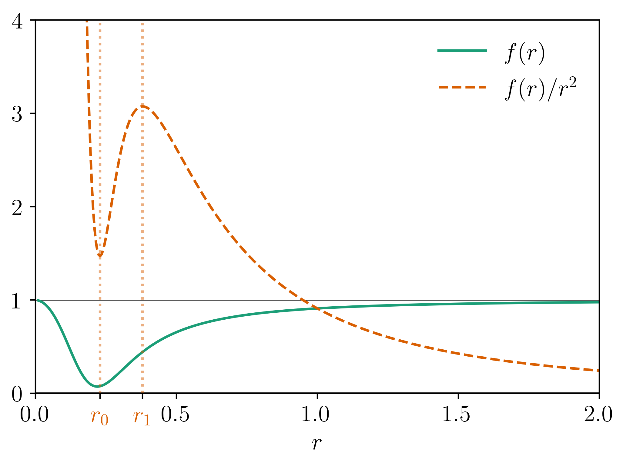
Figure 1: We choose the scalar function $f(r)=1-r^{2}(0.026+11.21\,r^{4})^{-1}$ (solid green line). The choice of $f(r)$ is such that the local minimum of the geodesic potential $V(r)=f(r)r^{-2}$ (dashed orange line) is located sufficiently close to the origin (i.e., $r_{0}\sim 0.22$) to guarantee the necessary numerical resolution within the stable trapping region (see Section V).

The spacetime $(\mathcal{M},g)$ is the model spacetime considered for the remainder of this work.

III Linear waves on the model spacetime

We consider the scalar linear wave equation

$$\Box_{g}\phi=0$$ (10)

for scalar functions $\phi:\mathcal{M}\rightarrow\mathbb{R}$ on the model spacetime $(\mathcal{M},g)$ of Section II.

Let $k\in\mathbb{N}$, with $k\geq 1$. We introduce the $k$-th order energies

$$\mathbb{E}^{k}[\phi](\tau)= \,\int_{t=\tau}dr\,d\vartheta\,d\varphi\,\frac{r^{2}\sin\vartheta}{2\,f(r)}$$ (11)

$$\times\sum_{0\leq|\alpha|\leq k-1}\left[(\partial_{t}\partial^{\alpha}\phi)^{2}+f^{2}(r)\,(\partial_{r}\partial^{\alpha}\phi)^{2}+\frac{f(r)}{r^{2}}\,(\partial_{\vartheta}\partial^{\alpha}\phi)^{2}+\frac{f(r)}{r^{2}\sin^{2}\vartheta}\,(\partial_{\varphi}\partial^{\alpha}\phi)^{2}\right]\,,$$

where we use the standard multi-index notation for $\alpha$. The order $k$ of the energy coincides with the order of the top-order derivatives of the solution appearing in the energy. We will denote $\mathbb{E}^{1}[\phi](t)=\mathbb{E}[\phi](t)$, with

$$\mathbb{E}[\phi](\tau)=\int_{t=\tau} dr\,d\vartheta\,d\varphi\,\frac{r^{2}\sin\vartheta}{2\,f(r)}$$ (12)

$$\times\left[(\partial_{t}\phi)^{2}+f^{2}(r)\,(\partial_{r}\phi)^{2}+\frac{f(r)}{r^{2}}\,(\partial_{\vartheta}\phi)^{2}+\frac{f(r)}{r^{2}\sin^{2}\vartheta}\,(\partial_{\varphi}\phi)^{2}\right]\,.$$

For any $t$-invariant set $\Omega\subset\mathcal{M}$ such that $\Omega\cap\left\{t=\tau\right\}$ is non-empty and bounded (for all $\tau\in\mathbb{R}$), we introduce the $k$-th order local energies $\mathbb{E}^{k}_{\Omega}[\phi](t)$, for which the integral (11) is now taken over the bounded region $\Omega\cap\left\{t=\tau\right\}$. We will denote $\mathbb{E}^{1}_{\Omega}[\phi](t)=\mathbb{E}_{\Omega}[\phi](t)$.

The following theorem summarises the uniform dynamics of linear waves on $(\mathcal{M},g)$. The set $\Omega$ invoked in the theorem is assumed to satisfy the properties described above.

Theorem 1.

For any $k\in\mathbb{N}$, with $k\geq 1$, and any set $\Omega$, there exist real constants $B_{k},C_{\Omega,k}>0$ such that, for any smooth, compactly supported initial data $(\phi,\partial_{t}\phi)|_{t=0}$ prescribed at $t=0$, the smooth solution $\phi$ to (10) satisfies the following properties:

• (Global existence) The solution $\phi$ exists and is unique for all $t\geq 0$.

• (Conservation of energy) The equality

  $$\mathbb{E}[\phi](t)=\mathbb{E}[\phi](0)$$

  holds for all $t\geq 0$.

• (Uniform energy boundedness) The inequality

  $$\mathbb{E}^{k}[\phi](t)\leq B_{k}\,\mathbb{E}^{k}[\phi](0)$$ (13)

  holds for all $t\geq 0$.

• (Uniform local energy decay, [14]) The inequality

  $$\mathbb{E}^{k}_{\Omega}[\phi](t)\leq\frac{C_{\Omega,k}}{[\log(2+t)]^{2}}\,\mathbb{E}^{k+1}[\phi](0)$$ (14)

  holds for all $t\geq 0$. Moreover, the logarithmic uniform energy decay rate is sharp.

Furthermore, uniform boundedness and uniform (sharp-)logarithmic decay for the solution and (higher-order) derivatives of the solution hold pointwise.

The first three bullet points in Theorem 1 are rather straightforward to prove. We note, in particular, that the uniform energy boundedness claimed in the third bullet point is, for the case $k=1$, an immediate consequence of the conservation of energy from the second bullet point. The decay statement of the last bullet point can be recovered as a special case of the more general result [14], which establishes an analogous energy decay statement for a class of static, spherically symmetric and asymptotically flat spacetimes (see Theorems 4.7 and 5.3 of [14], and Corollary 5.4 therein for a pointwise decay statement). The sharpness of the logarithmic uniform energy decay rate is to be directly ascribed to the presence of stably trapped null geodesics on $(\mathcal{M},g)$ and can be proven by applying the quasimode construction of [14]. Finally, we note that, for $k=1$, the local energy decay is compatible with the conservation of energy stated in the second bullet point, and in fact it encodes the dispersion of solutions.

While the local energy of the generic (possibly axisymmetric) solution decays only logarithmically in time, the local energy decay rate of solutions supported on a finite number of angular modes (including, in particular, spherically symmetric solutions) is faster. Indeed, by decomposing solutions into spherical harmonics $Y^{\ell}_{m}(\vartheta,\varphi)$, i.e.,

$$\phi(t,r,\vartheta,\varphi)=\frac{1}{\sqrt{2\pi}}\sum_{\ell\geq 0,|m|\leq\ell}\phi_{\ell m}(t,r,\vartheta,\varphi)$$

with $\phi_{\ell m}(t,r,\vartheta,\varphi)=b_{\ell m}(t,r)Y^{\ell}_{m}(\vartheta,\varphi)$, one can prove that the local energy of each angular mode $\phi_{\ell m}$ decays with an integrable rate, i.e., the integrated local (for any $\Omega$) energy decay estimate

$$\int_{0}^{\infty}\mathbb{E}_{\Omega}[\phi_{\ell m}](t)\,dt\leq C_{1}e^{C_{2}\sqrt{\ell(\ell+1)}}\,\mathbb{E}[\phi_{\ell m}](0)$$ (15)

holds, with positive constants $C_{1}$ and $C_{2}$ independent of $\ell$ (cf. Theorem 5.1 in [14]). Similar considerations hold for local higher-order energies. Crucially, the inequality (15) degenerates as $\ell\rightarrow\infty$, encoding the fact that (i) the decay of the local energy is slower for high-frequency angular modes and (ii) the inequality degenerates for the generic solution (i.e., for infinite sums of angular modes). Indeed, the logarithmic decay rate of the generic solution is non-integrable.

IV The model nonlinear wave equation

We consider the cubic (defocusing) wave equation

$$\Box_{g}\phi=\phi|\phi|^{2}$$ (16)

for scalar functions $\phi:\mathcal{M}\rightarrow\mathbb{R}$ on the model spacetime $(\mathcal{M},g)$ of Section II.

We introduce the (first-order) energy

$$\mathbb{E}_{\text{nl}}[\phi](\tau)=\int_{t=\tau} dr\,d\vartheta\,d\varphi\,\frac{r^{2}\sin\vartheta}{2\,f(r)}$$ (17)

$$\times\left[(\partial_{t}\phi)^{2}+f^{2}(r)\,(\partial_{r}\phi)^{2}+\frac{f(r)}{r^{2}}\,(\partial_{\vartheta}\phi)^{2}+\frac{f(r)}{r^{2}\sin^{2}\vartheta}\,(\partial_{\varphi}\phi)^{2}+f(r)\,\frac{|\phi|^{4}}{2}\right]\,.$$

We state a large-data global existence theorem for solutions to the equation (16). As in the linear case (cf. Theorem 1), the equation (16) admits global-in-time smooth solutions and a conserved energy.

Theorem 2.

For any smooth, compactly supported initial data $(\phi,\partial_{t}\phi)|_{t=0}$ prescribed at $t=0$, the smooth solution $\phi$ to (16) satisfies the following properties:

• (Global existence) The solution $\phi$ exists and is unique for all $t\geq 0$.

• (Conservation of energy) The equality

  $$\mathbb{E}_{\textup{nl}}[\phi](t)=\mathbb{E}_{\textup{nl}}[\phi](0)$$

  holds for all $t\geq 0$.

The second bullet point in Theorem 2 is an easy check, whereas the first bullet point can be, for instance, recovered as a special case of the more general result [42]. We emphasise that Theorem 2 does not require any smallness assumption on the size of the initial data. For equation (16), global existence is directly implied by the conservation (and coercivity) of the energy (combined with a standard Sobolev embedding). In particular, linear decay does not play any role. We also remark that the conservation of the energy (17) implies a uniform bound on first derivatives of solutions, but remains compatible with (possibly unbounded) growth of high-order derivatives.

For future convenience, we define the Fourier coefficient

$$c_{\ell}(t,r)=2\pi r^{2}\int_{0}^{\pi}\phi\left(t,r,\vartheta\right)\cdot Y_{0}^{\ell}\left(\vartheta\right)\sin\vartheta\,d\vartheta$$ (18)

for any given axisymmetric solution to equation (16). We also define the Fourier coefficient

$$\tilde{c}_{\ell}(t,r)=2\pi r^{2}\int_{0}^{\pi}\phi^{3}\left(t,r,\vartheta\right)\cdot Y_{0}^{\ell}\left(\vartheta\right)\sin\vartheta\,d\vartheta$$ (19)

for the cubic power of the solution. By Fourier-decomposing the solution, one can write the energy (17) as

$$\mathbb{E}_{\text{nl}}[\phi](t)= \,\frac{1}{2\pi}\sum_{\ell}\int_{0}^{\infty}dr\,\frac{r^{2}}{2\,f(r)}\left[(\partial_{t}c_{\ell})^{2}+f^{2}(r)\,(\partial_{r}c_{\ell})^{2}+b\,\frac{f(r)}{r^{2}}\,\ell(\ell+1)c^{2}_{\ell}\right]$$ (20)

$$+\frac{1}{8\pi}\sum_{\ell}\int_{0}^{\infty}dr\,r^{2}\,\tilde{c}_{\ell}\,c_{\ell}$$

for some constant $b>0$ independent of $\ell$, where the term in the second line of (20) is positive (as it arises from the positive last term in (17)). By defining the energy quantity

$$\mathbb{E}_{\ell}[\phi](t)= \,\frac{1}{2\pi}\int_{0}^{\infty}dr\,\frac{r^{2}}{2\,f(r)}\left[(\partial_{t}c_{\ell})^{2}+f^{2}(r)\,(\partial_{r}c_{\ell})^{2}+b\,\frac{f(r)}{r^{2}}\,\ell(\ell+1)c^{2}_{\ell}\right]$$ (21)

$$+\frac{1}{8\pi}\int_{0}^{\infty}dr\,r^{2}\,\tilde{c}_{\ell}\,c_{\ell}\,,$$

which may be interpreted as the “energy of the $\ell$-angular mode”, the conservation of the energy (17) yields

$$\sum_{\ell}\mathbb{E}_{\ell}[\phi](t)=\mathbb{E}_{\text{nl}}[\phi](0)$$ (22)

for all $t\geq 0$.

V Numerical implementation

To numerically solve equation (16), we start by re-writing the equation in the form

$$\frac{1}{\sqrt{-g}}\left(\sqrt{-g}g^{\mu\nu}\phi_{,\mu}\right)_{,\nu}=\phi^{3}\,.$$

We consider the auxiliary scalar quantity

$$\Pi=-g^{t\mu}\phi_{,\mu}\,.$$

Equation (16) can then be recast as a system of two evolution equations which are of first order in the time variable, i.e.,

$$\phi_{,t} =-\frac{\Pi+g^{ti}\phi_{,i}}{g^{tt}}\,,$$ (23)

$$\Pi_{,t} =\frac{1}{\sqrt{-g}}\left[-\left(\sqrt{-g}\right)_{,t}\Pi+\left(\sqrt{-g}g^{ij}\phi_{,i}\right)_{,j}\right.$$

$$\phantom{=}\left.-\left(\sqrt{-g}g^{it}\left(\frac{\Pi+g^{tk}\phi_{,k}}{g^{tt}}\right)\right)_{,i}-\sqrt{-g}\phi^{3}\right].$$ (24)

The quantity $\Pi_{,t}$ will be sometimes denoted by $\dot{\Pi}$.

As a preliminary step, we transform our spatial coordinates from spherical ($r,\vartheta,\varphi$) to standard Cartesian coordinates $(x,y,z)$. In particular, $\varphi$ is treated as the azimuthal angle relative to the $z$-axis and the origins of the two coordinate systems coincide. We discretise the spatial derivatives using standard fourth-order finite differences, evolve in time with a standard fourth-order Runge–Kutta method, and, for stability purposes, we add numerical dissipation through standard Kreiss–Oliger dissipation operators [43] to the right hand sides of the equations (23)-(24).

To achieve sufficiently high resolution for the numerical evolution with limited computational resources, we assume that the solution is axisymmetric. Together with the axisymmetry of the background spacetime, the symmetry class of the solutions allows one to apply the so-called modified Cartoon method [44, 45] and evolve the system of equations (23)-(24) on a $2+1$ dimensional computational domain (the spacetime is still $3+1$ dimensional). The dimensional reduction is implemented as follows:

• We write the azimuthal Killing vector field $\xi$ of the background spacetime as

  $$\xi=-y\,\frac{\partial}{\partial x}+x\,\frac{\partial}{\partial y}\,,$$

  meaning that we choose the axis of symmetry to coincide with the $z$-axis.

• Let

  $$\mathcal{P}\cong\left\{0\right\}_{x}\times[0,\infty)_{y}\times(-\infty,\infty)_{z}\,.$$

  Once initial data are prescribed at $t=0$, we numerically solve the equations (23)-(24) in the spacetime region $\mathcal{C}\subset\mathcal{M}$ such that

  $$\mathcal{C}\cong[0,\infty)_{t}\times\mathcal{P}\,.$$

• We reconstruct the derivatives with respect to $x$ on $\mathcal{C}$, which can, in fact, be written in terms of the derivatives with respect to $y$ and $z$ by exploiting the identities for Lie derivatives

  $$\mathcal{L}_{\xi}g =0\,, \mathcal{L}_{\xi}\phi =0\,.$$

  The reconstruction procedure uses, in particular, the property that $\xi$ is nowhere tangent to $\mathcal{P}$ (see [44] for the relevance of this fact).

• Using the axisymmetry of the solution, the solution can then be extended from $\mathcal{C}$ to the whole spacetime $\mathcal{M}$.

As an auxiliary step, we also compactify the spatial coordinates while going through the dimensional-reduction procedure. Indeed, the equations (23)-(24) are evolved in compactified Cartesian coordinates $\left(t,X,Y,Z\right)$, with

$$X \in[-1,1]\,, Y \in[-1,1]\,, Z \in[-1,1]\,,$$

obtained via the coordinate transformation

$$X= \frac{2}{\pi}\arctan x\,, Y= \frac{2}{\pi}\arctan y\,, Z= \frac{2}{\pi}\arctan z\,.$$ (25)

In the compactified coordinates, we have

$$\mathcal{P}\cong\left\{0\right\}_{X}\times[0,1]_{Y}\times[-1,1]_{Z}\,.$$ (26)

Since the compactification includes spacelike infinity, the asymptotically flat boundary condition is applied by enforcing the Minkowski space values for the metric, and that the field goes to zero. On the other hand, since we are working on the $X=0$ slice, on-axis regularity conditions are necessary and prescribed following [44].

VI Numerical results

In this section, we present the results of our numerical simulations. We focus on three aspects of numerical solutions to equation (16), each discussed in a distinct section: The growth of high-order derivatives (Section VI.3), the direct angular-mode cascade (Section VI.4), and the evolution of small initial data (Section VI.5).

VI.1 Initial data

The solutions considered arise as the future evolution of time-symmetric initial data of the form

$$\phi|_{t=0} =\epsilon\,u(r)\cdot\sum_{\left[\ell\right]}Y_{0}^{\ell}(\vartheta)\,, \partial_{t}\phi|_{t=0} =0\,,$$ (27)

where $\epsilon$ is a positive real constant. The scalar function $u(r)$ is compactly supported on a finite interval $[r_{0,1},r_{0,2}]$ around $r=r_{0}$ (cf. Figure 1) and will be chosen to be smooth on its support (but only finitely differentiable on $r\in(0,\infty)$). The scalar functions $Y_{0}^{\ell}(\vartheta)$ denote the standard spherical harmonics $Y_{m}^{\ell}(\vartheta,\varphi)$ of the unit $2$-sphere with $m=0$, and $\left[\ell\right]$ symbolizes the set of spherical harmonics considered (e.g., $\left[\ell_{1},\ell_{2}\right]$ in (27) would denote the sum $Y_{0}^{\ell_{1}}(\vartheta)+Y_{0}^{\ell_{2}}(\vartheta)$). We will only consider initial data containing finite sums of spherical harmonics.

The initial data (27) are axisymmetric. The axisymmetry of the initial data is preserved by equation (16), and thus the solution remains axisymmetric for all future times.

VI.2 Intermezzo: Linear decay

The linear solutions arising from initial data of the form prescribed in Section VI.1 can be written as finite sums of (axisymmetric) angular modes. As discussed in Section III, the uniform decay rate of the local energy of these solutions, as well as of their local higher-order energies, is faster than for the generic solution. In this respect, since the nonlinear turbulent dynamics that we shall describe is favoured by slow linear decay, the turbulent behaviour of the initial data prescribed in Section VI.1 may be expected to persist for more general, perhaps generic, initial data. See the related discussion in Section VII.1.

VI.3 Growth of high-order derivatives

We consider numerical solutions to equation (16). For the numerical simulations of the present section, we choose our “canonical” initial data (27) to be

$$u(r)=4000\cdot\frac{\left(r-r_{0,1}\right)^{4}\left(r-r_{0,2}\right)^{4}}{\left(r_{0,1}-r_{0,2}\right)^{8}}$$ (28)

for $r\in[r_{0,1},r_{0,2}]$ (see Figure 2), and with parameters

$$\epsilon =1\,, r_{0,1} =0.02\,, r_{0,2} =0.6\,, [\ell] =[1,2].$$ (29)

The results shown in this (and the following) section(s) are run on a grid of resolution $(\Delta_{Y},\Delta_{Z})=0.003125$, with a Courant factor $C=0.5$ (i.e., $\Delta_{t}=0.5\,\Delta_{Y}$). We have applied a sixth-order Kreiss–Oliger dissipation, with $\epsilon_{\rm KO}=0.3$ for numerical stability. The convergence tests of all the simulations presented are collected in Appendix B.

The selection of $\epsilon=1$ in (29) ensures that the nonlinearity of equation (16) significantly influences the dynamics of the solution during the initial stages, reducing the need for very long evolutions. This behavior is illustrated in Figure 3 for one quantity of interest ((31) below), where we display the results from the evolution of $\epsilon=1$-initial data compared to the evolution of several different initial amplitudes around this value. A solution dominated by the linear dynamics should exhibit similar behavior for different initial amplitudes (modulo an overall scale proportional to $\epsilon$). This is evident for the $\epsilon=0.125$ vs. $\epsilon=0.25$ cases plotted in the figure, but notably begins to fail increasing $\epsilon$ to values close to $1$. The remainder of this section focuses on amplitudes around $\epsilon=1$; for a discussion of the evolution of smaller amplitude initial data, see Section VI.5.

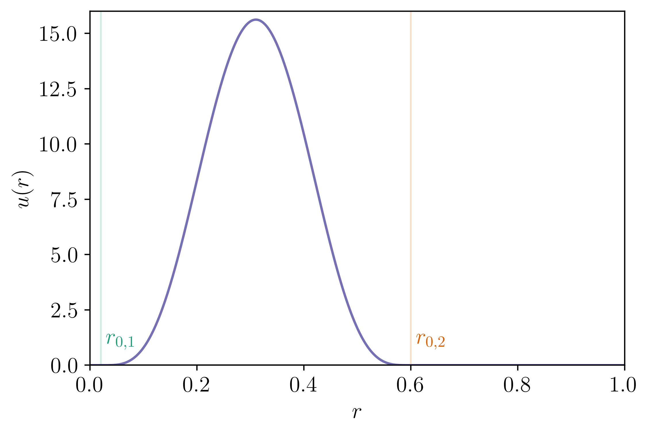
Figure 2: The function $u(r)$ as defined for the initial data in (28). We recall that the minimum of the radial geodesic potential $V(r)$ is located at $r_{0}\sim 0.22$ (cf. Figure 1).

Figure 3: The evolution of the quantity (31) over the time interval $t\in[0,3]$, with a logarithmic scale on the vertical axis. Six different values of $\epsilon$ are examined, each corresponding to a different color in the plot. For $\epsilon=0.75$ or larger, the solution already exhibits a markedly nonlinear behaviour within the time interval considered. The convergence of these simulations is shown in Figure 17.

Figure 4: Time snapshots of the evolution of the solution $\phi$ on the spatial domain $\mathcal{P}$ (recall (26)) over the time interval $t\in[0,150]$. For different snapshots, time increases from the left to the right (top to bottom). The vertical axis and color correspond to the amplitude of the solution, with orange depicting positive values of the solution and green negative values. The range of the vertical axis varies from one panel to another.

Figure 5: The evolution of the quantity (30) over the time interval $t\in[0,150]$, with a logarithmic scale on the vertical axis. The point-wise relative numerical error in this quantity is generally sub-percent level (see Appendix B for more details).

Figure 6: The evolution of the quantity (31) over the time interval $t\in[0,150]$, with a logarithmic scale on the vertical axis (note the different range of the axis from Figure 5). The point-wise relative numerical error in this quantity is generally sub-percent level (see Appendix B for more details).

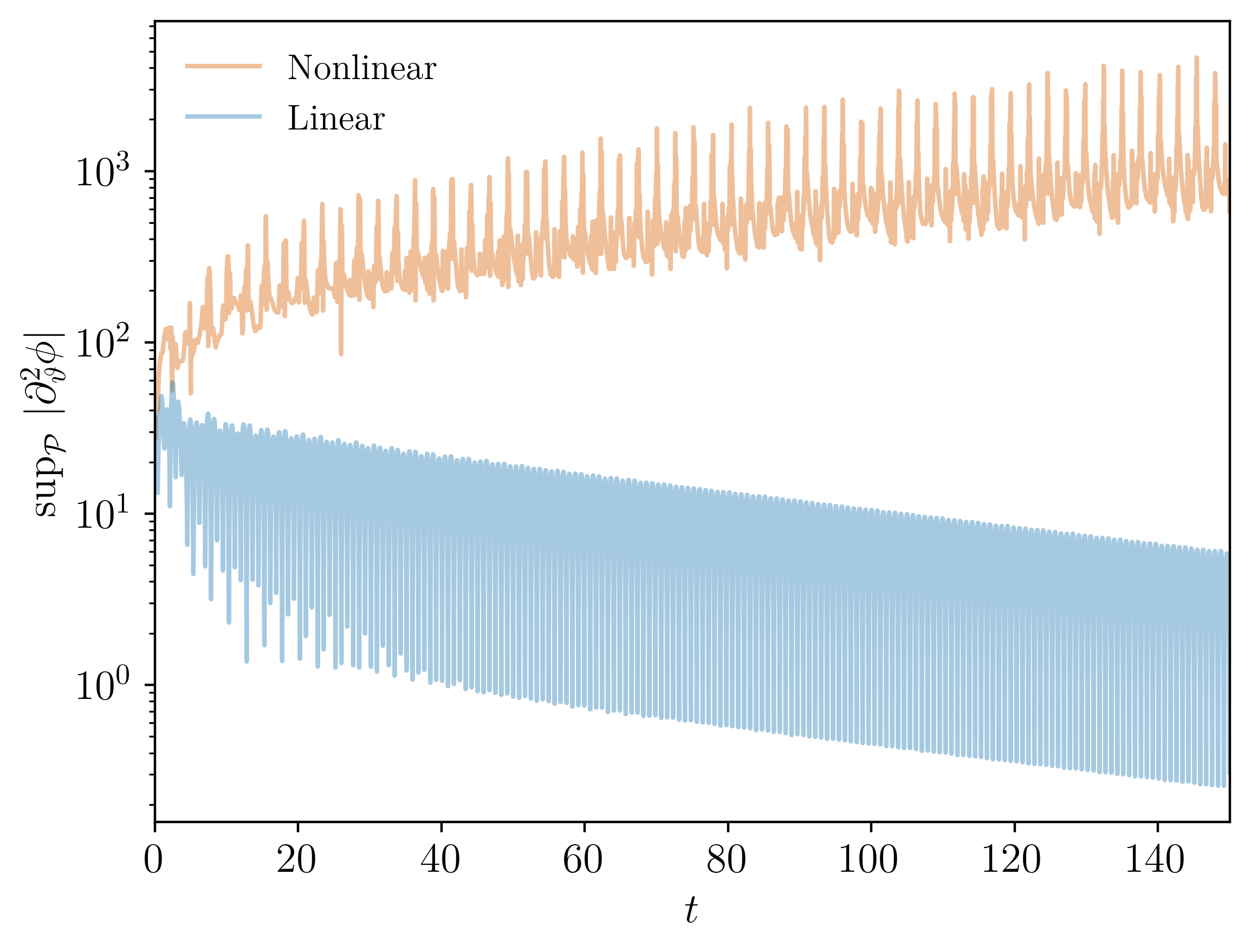
Figure 7: The evolution of the quantity (31) over the time interval $t\in[0,150]$, with a logarithmic scale on the vertical axis. We consider the solution to the linear wave equation (10) (blue line) and the solution to the nonlinear wave equation (16) (orange line), both arising from the initial data considered in Section VI.3. The orange line coincides with the one plotted in Figure 6.

Figure 8: The evolution of the quantity (30) over the time interval $t\in[0,150]$, with a logarithmic scale on the vertical axis. The three values $\epsilon=\{0.75,1,1.25\}$ are examined, each corresponding to a different color in the plot (green, orange and purple, respectively). The convergence of these simulations is shown in Figure 18.

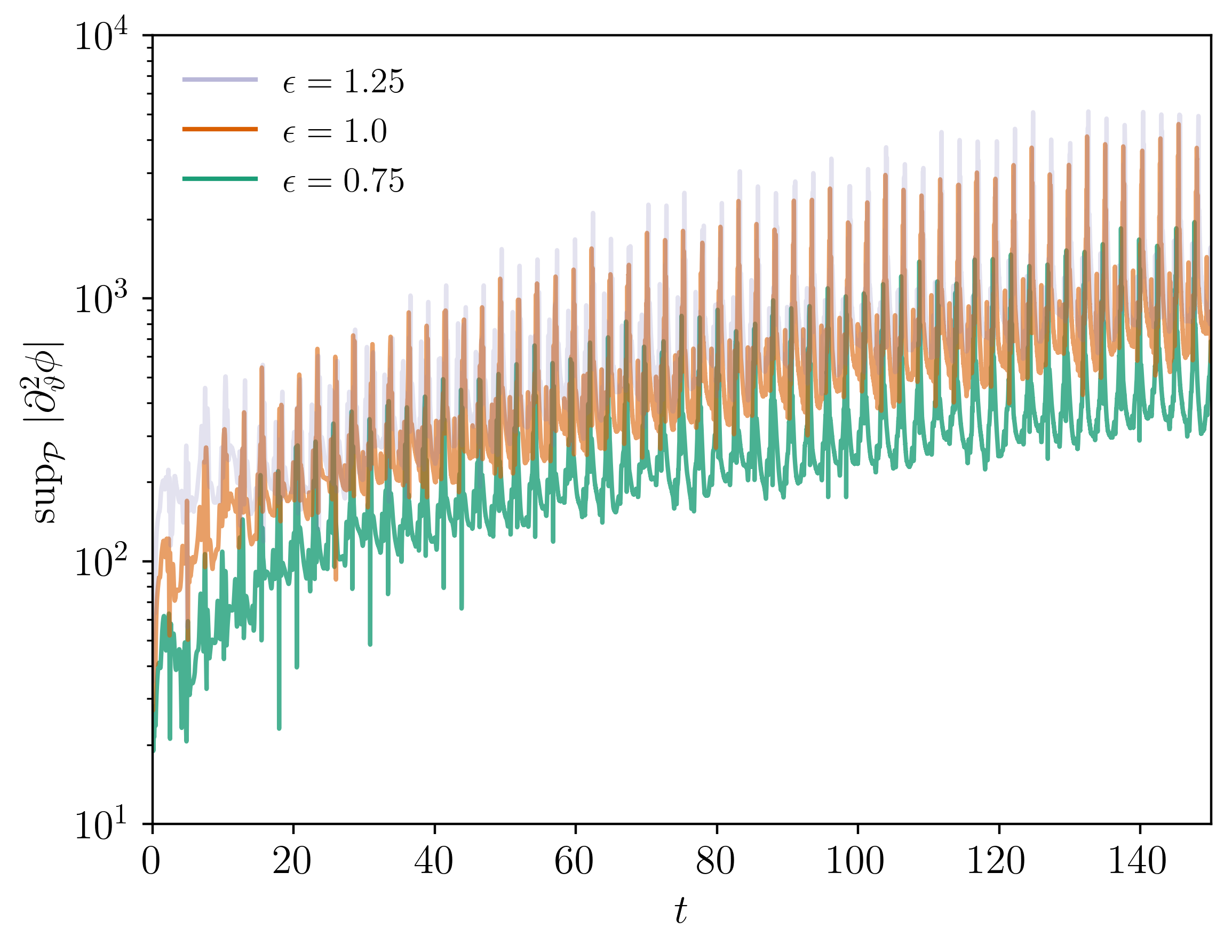
Figure 9: The evolution of the quantity (31) over the time interval $t\in[0,150]$, with a logarithmic scale on the vertical axis. The three values $\epsilon=\{0.75,1,1.25\}$ are examined, each corresponding to a different color in the plot (green, orange and purple, respectively).

Figure 4 shows the numerical evolution of the solution $\phi$. While the solution disperses (with its amplitude decaying over time), part of the solution remains confined within the stable trapping region over the entire interval of time that we evolve. Within the stable trapping region, the solution appears to develop high-frequency structure, already hinting at a possible growth of its high-order derivatives.

Figure 5 tracks the numerical evolution of the quantity

$$\sup_{\mathcal{P}}|\dot{\Pi}|(t)\,,$$ (30)

where we recall the definition of $\mathcal{P}$ from (26). The quantity (30) is seen to grow over the entire time interval considered. Second spatial derivatives exhibit an analogous behaviour as the one showed in Figure 5. For instance, Figure 6 examines the numerical evolution of the quantity

$$\sup_{\mathcal{P}}|\partial_{\vartheta}^{2}\phi|(t)\,,$$ (31)

which also grows over the entire time interval considered. We note that the growth of the quantities (30) and (31) is intended upon averaging over an appropriate timescale, as it is apparent from the figures. From the dynamics of the solution observed in Figure 4 and the fact that an analogous behaviour for the quantities (30) and (31) can be seen to persist when the supremum is only taken over the stable trapping region, we conclude that the growth of the second derivatives captured by Figures 5 and 6 occurs within (and is tied to the presence of) the stable trapping region. Moreover, we remark that the growth of second-order derivatives is a genuinely nonlinear phenomenon. The difference between linear and nonlinear evolution of second-order derivatives is illustrated in Figure 7 for the quantity (31). For the same initial data prescribed for Figure 6, the quantity (31) associated to the linear solution can be seen to decay over the time interval considered (as predicted by Theorem 1 and discussed in Section VI.2).

For illustration, in Figures 8 and 9 we show the quantities (30) and (31) respectively from numerical evolution of the same form of initial data just discussed, but now including two additional choices of initial amplitude $\epsilon=0.75$ and $\epsilon=1.25$. Both plotted quantities grow throughout the time interval considered, with a similar growth rate for all three values of $\epsilon$. To go beyond a crude comparison of growth trends and investigate the possible presence of a scaling relation for the growing quantities (30) and (31) within our class of initial data, one would need to carry out additional numerical simulations over a range of values of $\epsilon$ covering several orders of magnitude, and possibly over much longer timescales than presented here (see also Section VI.5 and the related comments therein).

Although not displayed here, we have also examined some additional higher (than second) order derivatives of the solution (in the $\epsilon=1$-case) and observed a similar behaviour to the one described for second derivatives.

VI.4 Direct angular-mode cascade

In this section, we show that the growth of high-order derivatives described in Section VI.3 is the result of a direct angular-mode cascade within our numerical solutions. To capture the mode cascade, we shall consider the Fourier coefficients $c_{\ell}(t,r_{0})$ and $\tilde{c}_{\ell}(t,r_{0})$, where we recall the definitions (18)-(19) and that $r=r_{0}$ corresponds to the location of the local minimum of the radial geodesic potential (see Figure 1).

Given a (axisymmetric) solution to equation (16) arising from the initial data (27) with the choices (29)-(28) of Section VI.3, we preliminarily observe that

$$\partial_{t}c_{\ell}(t,r_{0})|_{t=0}=0$$

and, using equation (16) and the form of the initial data considered, we compute

$$\partial_{t}^{2}c_{\ell}(t,r_{0})|_{t=0}=F_{r_{0}}\delta_{\ell}^{1}+H_{r_{0}}\delta_{\ell}^{2}-f(r_{0})\cdot\tilde{c}_{\ell}(0,r_{0})\,,$$ (32)

with $\delta_{i}^{j}$ denoting the Kronecker delta, and the constants $F_{r_{0}}$ and $H_{r_{0}}$ are

$$F_{r_{0}} =2\pi r_{0}f(r_{0})\cdot(\partial_{r}(rf(r)\partial_{r}u(r)))(r_{0})+4\pi f(r_{0})u(r_{0})\,,$$

$$H_{r_{0}} =2\pi r_{0}f(r_{0})\cdot(\partial_{r}(rf(r)\partial_{r}u(r)))(r_{0})+12\pi f(r_{0})u(r_{0})\,.$$

Since the initial data are supported on $\ell\in[1,2]$, the non-trivial values of $\tilde{c}_{\ell}(0,r_{0})$ in (32) correspond to $\ell\in[0,\dots,6]$ (see Figure 10), as one can compute using the Clebsch–Gordan coefficients. The quantity (32) is therefore non-trivial for $\ell\in[0,\dots,6]$.

The time evolution of the $\ell$-spectrum of the numerical solution is depicted in Figure 11. In agreement with the prescribed initial data, the solution is only “supported” on the $\ell\in[1,2]$-angular modes at $t=0$, with $c_{1}(0,r_{0})=c_{2}(0,r_{0})\sim 3.2$. At time $t=0.01$, the numerical solution is supported on the wider range of angular modes with $\ell\in[0,\dots,14]$. At this time, the newly excited modes above the numerical floor appear to be grouped into sequences whose Fourier coefficients take approximately the same value. We shall refer to such sequences as generations. The first generation of modes consists of modes with $\ell=0$ and $\ell\in[3,\dots,6]$, which are excited to larger amplitude than the modes with higher $\ell\in[7,\ldots,14]$. In fact, as encoded by equation (32), the first generation of excited modes of Figure 11 is driven, for small times (i.e., $t=0.01$ in Figure 11), by the $\ell$-spectrum of the cubic power $\phi^{3}(0,r_{0},\vartheta)$ of the initial datum, which is indeed supported on angular modes with $\ell\in[0,\ldots,6]$ (see Figure 10). By time $t=0.1$, all the angular modes with $\ell\in[0,\dots,15]$ are excited above the numerical floor. Approaching $t=100$, the curve connecting the points in Figure 11 progressively flattens, with the excited $\ell\in[5,\dots,15]$-angular modes reaching their maximum amplitude (within our evolution) and attaining approximately the same amplitude as the $\ell\in[1,2]$-angular modes. After $t=100$, all the excited angular modes depicted appear to settle down to an almost stationary regime (see the small difference in amplitude of the modes between $t=100$ and $t=150$). Overall, we observe slow dispersion of the $\ell\in[1,2]$-angular modes over the entire evolution and slow dispersion of the excited $\ell\in[5,\dots,15]$-angular modes once they attain their maximum amplitude.

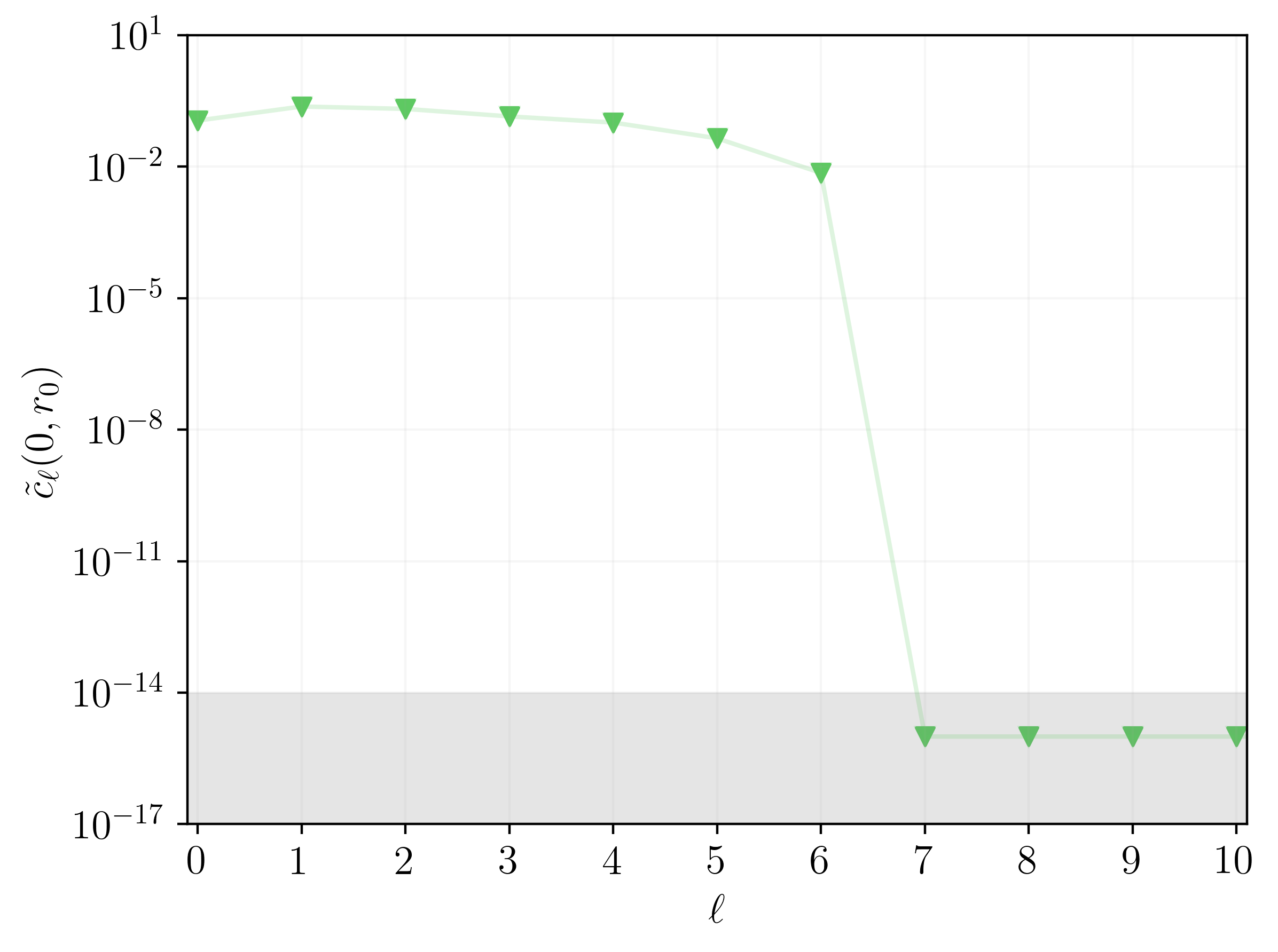
Figure 10: The $\ell$-spectrum of the cubic power $\phi^{3}$ of the solution at the initial time, as captured by the Fourier coefficients (19), with a logarithmic scale on the vertical axis. The grey shading indicates where the numerical floor of our simulations is. We note that the Fourier coefficients plotted are all positive, with no absolute value applied to the Fourier coefficients on the vertical axis.

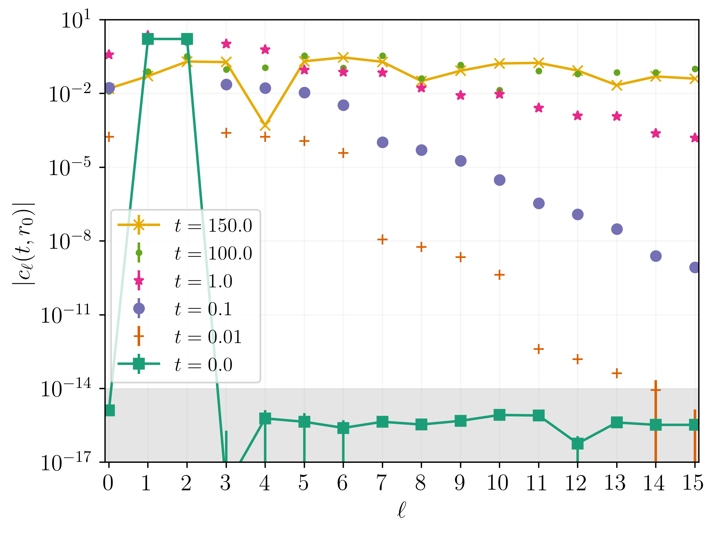
Figure 11: The $\ell$-spectrum of the solution at different times in the evolution, as captured by the Fourier coefficients (18), with a logarithmic scale on the vertical axis. Lines joining the points for the times $t=0$ and $t=150$ have been added to guide the reader. The grey shading indicates where the numerical floor of our simulations is. The numerical errors in the late time ($t=150$) quantities are on the order of $10^{-3}$ or less, as can be inferred from the resolution study shown in Figure 22. Note that the seemingly anomalous low value for the $l=4$-mode at $t=150$ is an artifact of us not averaging the amplitude coefficients in time over the local oscillation period of these modes, as illustrated in Figure 12 below (i.e., the evolution is near a local minimum of the $l=4$-mode at that time).

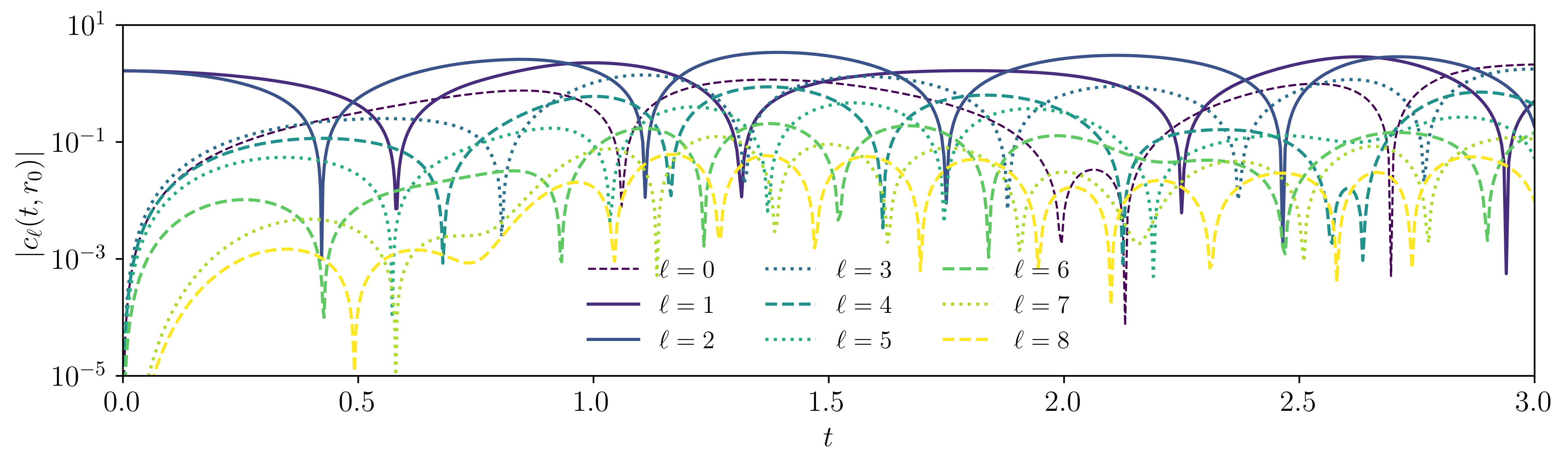
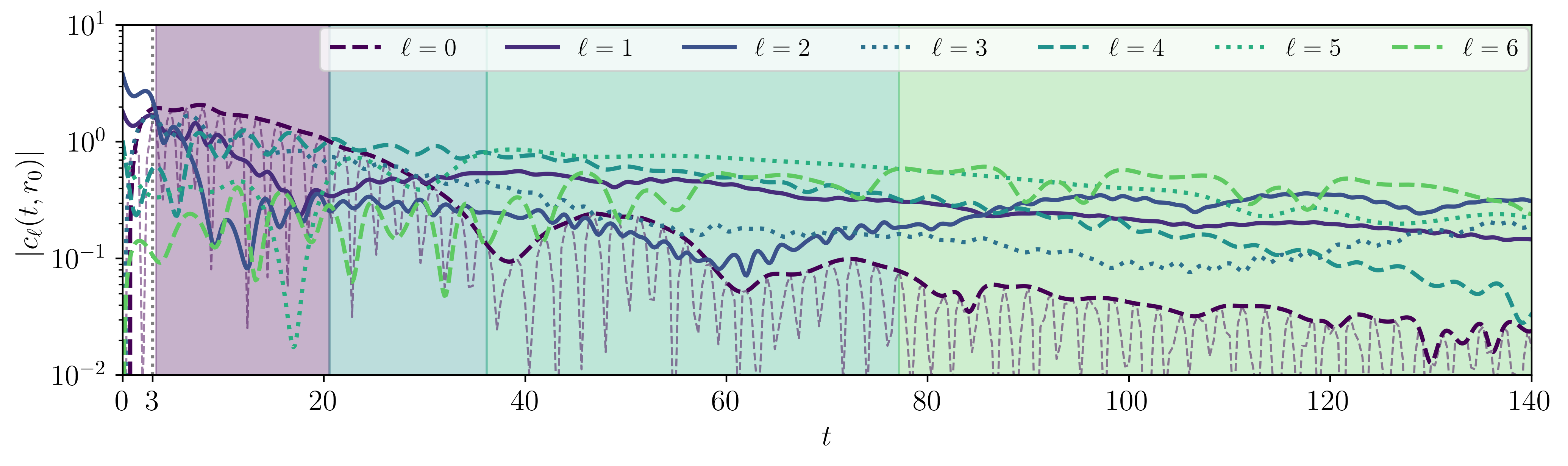
Figure 12: The time evolution of the Fourier coefficients (18) for $\ell\in[0,\dots,8]$ ($[0,\dots,6]$) in the top (bottom) panel, with logarithmic scales on the vertical axes. The top panel shows the evolution over the initial time interval $t\in[0,3]$, whereas the bottom panel displays the envelope of the evolution over the entire time interval $t\in[0,140]$ (the vertical dotted line in the bottom panel marks the time $t=3$, i.e., the end of the initial interval of time blown-up in the top panel). For illustrative purposes, in the bottom panel we have also plotted the instantaneously measure amplitude of the $\ell=0$-mode (thinner line) in addition to its envelope (thicker line); similar behaviour occurs for all modes. Note the different ranges of the vertical axes in the two panels, and that both the lower ends of the two ranges are several orders of magnitude above the numerical floor. The curves in the panels correspond to single values of $\ell$, which are identified by different colors. In the top panel, the $\ell\in[1,2]$-angular modes (shown with solid lines) are contained in the prescribed initial data and are displayed with their initial amplitude at $t=0$. The growth of the excited angular modes with $\ell=0$ and $\ell\in[3,\dots,6]$ can be seen to precede (in time) the growth of the excited angular modes with $\ell\in[7,8]$ (cf. the first and second generations of excited modes in Figure 11). In the bottom panel, the multi-colored background identifies the time intervals over which the correspondingly colored angular mode dominates. For $t\in[0,3.3]$, the $\ell\in[1,2]$-angular modes dominate the evolution. For the later times in the plot, the dominant angular modes are (in order) $\ell\in[0,4,5,6]$. The convergence of these coefficients at two different late times is shown in Figure 22.

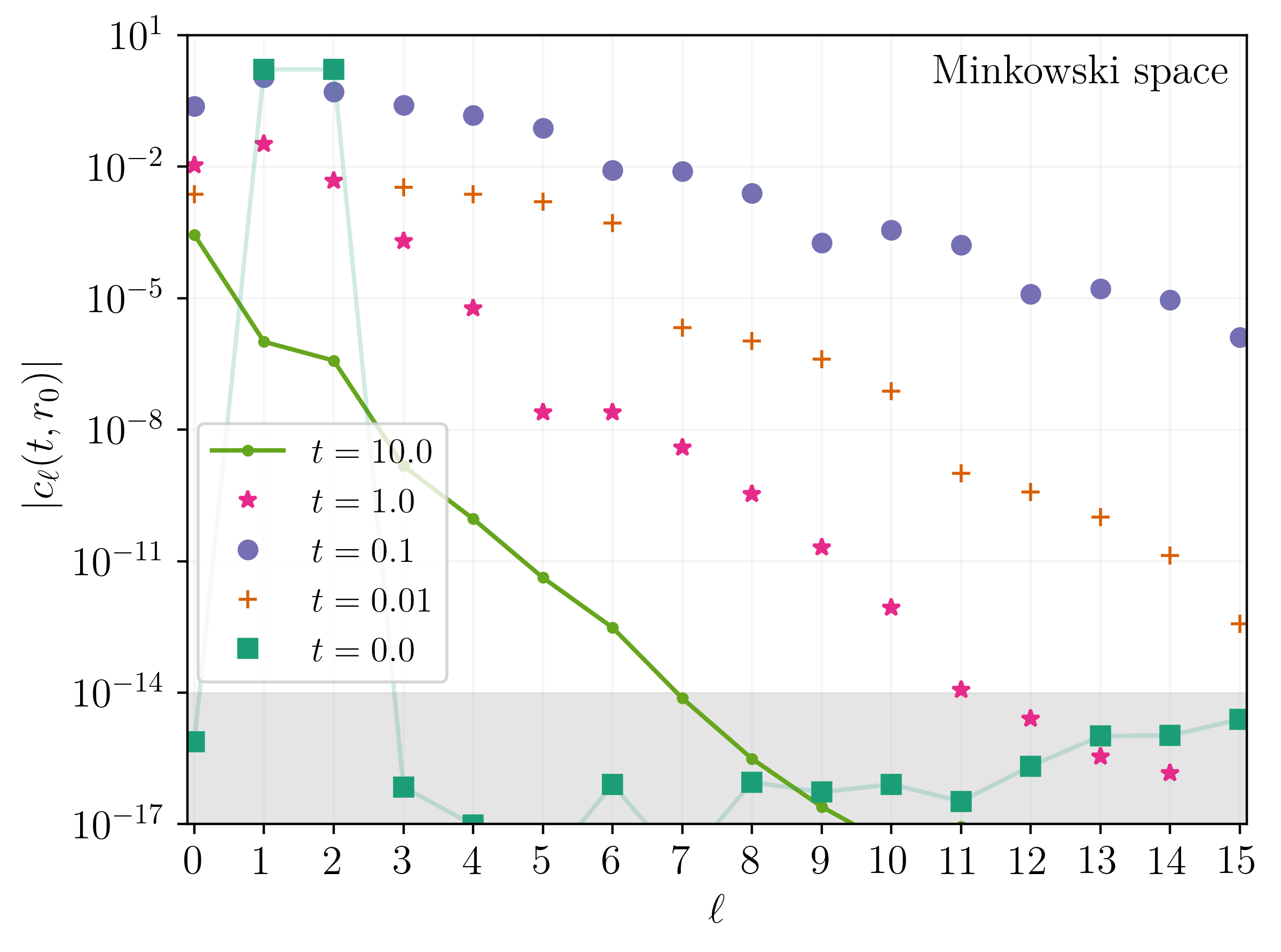
Figure 13: The $\ell$-spectrum of the solution to equation (6) on Minkowski space, arising from the same initial data considered for Figure 11. The $\ell$-spectrum is depicted at different times in the evolution, as captured by the Fourier coefficients (18), with a logarithmic scale on the vertical axis. Lines joining the points for the times $t=0$ and $t=10$ have been added to guide the reader. The grey shading indicates where the numerical floor of our simulations is. The reader may compare this figure with Figure 11, noting however the shorter times plotted here.

In Figure 12, we show a more detailed analysis of the time evolution of individual angular modes with $\ell\in[0,\dots,8]$ for the same numerical solution depicted in Figure 11. We observe that, not only do the excited angular modes attain approximately the same amplitude as the $\ell\in[1,2]$-modes over time (as already apparent from Figure 11), but progressively higher-$\ell$ excited angular modes come to dominate in the evolution. Moreover, the time interval over which an individual higher-$\ell$ excited mode dominates appears to dilate over the evolution (compare the different colored backgrounds in Figure 12).

From Figures 11 and 12, one can conclude that the numerical solution undergoes a low-to-high angular-mode cascade, which we shall refer to as direct or forward cascade. We remark that the direct angular-mode cascade implies a transfer of energy from low to high angular modes. Indeed, for $t=0$ we have

$$\sum_{\ell}\mathbb{E}_{\ell}[\phi](0)=\mathbb{E}_{\ell=1}[\phi](0)+\mathbb{E}_{\ell=2}[\phi](0)=\mathbb{E}_{\text{nl}}[\phi](0)$$

(recall definition (21)), whereas for $t>0$, as the higher angular modes get excited, there are energies $\mathbb{E}_{\ell}[\phi](t)$ for $\ell\geq 3$ which become non-zero. By the conservation identity (22), the excitation of the higher-mode energies implies an energy transfer from the initial lower-mode energies $\mathbb{E}_{\ell=1}[\phi](0)$ and $\mathbb{E}_{\ell=2}[\phi](0)$ (i.e., the quantity $\mathbb{E}_{\ell=1}[\phi](t)+\mathbb{E}_{\ell=2}[\phi](t)$ decreases over time).

In Appendix A, we show that a similar angular-mode cascade occurs for the (very) early time evolution of initial data of the same form as the ones considered in this section, but supported on different (finite) sums of low angular modes. There, in Figure 15, we observe that when the initial data contain more than two angular modes, the first generation consists of a correspondingly larger number of newly excited angular modes. Also, there are more excited modes in the first generation for initial data containing a single higher-frequency mode than for initial data containing a single lower-frequency mode. In addition to exciting a wider range of first-generation angular modes, we recall that higher-frequency angular modes are also characterised by a slower linear decay (see Section III), and are thus expected to be longer-lived in the nonlinear evolution (this aspect is not captured by Figure 15, which displays the various $\ell$-spectra only for short times). The combination of these elements supports the expectation that more general, perhaps generic, initial data, which are supported on all angular modes (in particular, on more angular modes and with higher frequency than the ones considered in this work), would still experience angular-mode dynamics with similar features to that described in this section. See also the related discussion in Section VII.1.

The accuracy of the values of the Fourier coefficients in Figures 10, 11, 12 and 13 (present section), Figure 14 (following section), and Figures 15 and 16 (Appendix A) depends on the choice of resolution for the numerical evolution of the solution and the precision of the interpolating procedure adopted to compute the integrals (18) and (19). The details of the former are discussed in Appendix B. For the latter, we have used a fifth-degree spline interpolator and an adaptive quadrature with tolerance set to $10^{-12}$. The resulting errors are very small, i.e., they are typically at least three orders of magnitude smaller than the values of the Fourier coefficients plotted (Figure 22 in Appendix B shows the numerical convergence of the Fourier coefficients for $\ell\in[1,\dots,15]$ for our canonical initial data case). We also note that the amplitude of the Fourier coefficients oscillate in time (as illustrated in Figure 12), and we have not performed any temporal averaging when presenting the data (nor, except for the bottom panel of Figure 12, do we show the envelope of the coefficients in time).

To conclude the section, we remark that the angular-mode cascade described is a genuinely nonlinear phenomenon which is tied to the presence of stable trapping. Indeed, the mixing of angular modes never occurs for linear waves and, in particular, for the linear wave equation (10) with initial data (27), each of the angular modes contained in the initial data decays rapidly in time (see Section VI.2 and compare with the evolution of the $\ell\in[1,2]$-angular modes in Figures 11 and 12). Moreover, although the mixing of angular modes typically occurs for nonlinear waves, the

• slow dispersion of the angular modes contained in the initial data,

• slow dispersion of the excited angular modes, once these attain their maximum amplitude, and

• dominance of progressively higher angular modes over increasingly longer intervals of time in the evolution,

starting from initial data containing a small number of low angular modes, are more characteristic features of nonlinear waves on our model spacetime. For example, solutions to equation (6) on Minkowski space (no trapping) or Schwarzschild exterior spacetimes (unstable trapping) would still exhibit the excitation of higher angular modes, but the excited modes, after attaining their maximum amplitude, would rapidly disperse; see Figure 13 for an example on a Minkowski background. As our Fourier coefficients are numerically computed within the stable trapping region (i.e., at $r=r_{0}$), one can ascribe the characteristic features of our mode cascade to the presence of stable trapping.

VI.5 Small-data analysis

In this section, we consider numerical solutions to equation (16) arising from the initial data prescribed in Sections VI.3 and VI.4 (i.e., (27) with the choices (28)-(29)), but now with two smaller initial amplitudes $\epsilon=0.125$ and $\epsilon=0.25$. We recall that, for these two amplitudes, the evolution at early times appears to be dominated by the linear dynamics (at least for the quantity plotted in Figure 3). We view the dynamics of the numerical solutions analysed in this section as a preliminary hint at the dynamics of solutions to equation (16) arising from small (amplitude) initial data of the form considered. In light of the results that we shall describe, one may speculate that the characteristic features of the angular-mode cascade of Section VI.4 would persist for arbitrarily small initial data of the form considered.

Indeed, for both $\epsilon=0.125$ and $\epsilon=0.25$, we observe a direct angular-mode cascade characterised by (i) the slow dispersion of the angular modes contained in the initial data, (ii) the slow dispersion of the excited angular modes, once these attain their maximum amplitude, and (iii) the dominance of progressively higher angular modes over the evolution (see Figure 14). For what concerns the dominance of higher angular modes over the angular modes contained in the initial data, we point out that, strictly speaking, only the $\ell=1$-mode gets dominated within the time interval evolved (in particular, at $t=150$, the $\ell\in[3,4]$-modes dominate the $\ell=1$-mode in both cases shown in Figure 14). In fact, when comparing the angular-mode cascades for these two smaller amplitudes, we note that the excitation of the higher angular modes becomes less efficient the smaller the amplitude of the initial data. For example, with the highest excited angular mode that we plot (i.e., $\ell=15$), the difference

$$|c_{\ell=2}(t,r_{0})|-|c_{\ell=15}(t,r_{0})|$$

at $t=150$ is larger for smaller $\epsilon$ (see also Figure 11 for a comparison with the $\epsilon=1$-case), resulting in steeper $t=150$-curves in Figure 14 for smaller $\epsilon$. Despite the decreased efficiency of the mode cascade, we speculate that, over a longer interval of time than the one numerically evolved, the higher angular modes will eventually dominate both the angular modes contained in the initial data, with the solution undergoing a qualitatively similar mode dynamics to the one illustrated in Figure 12.

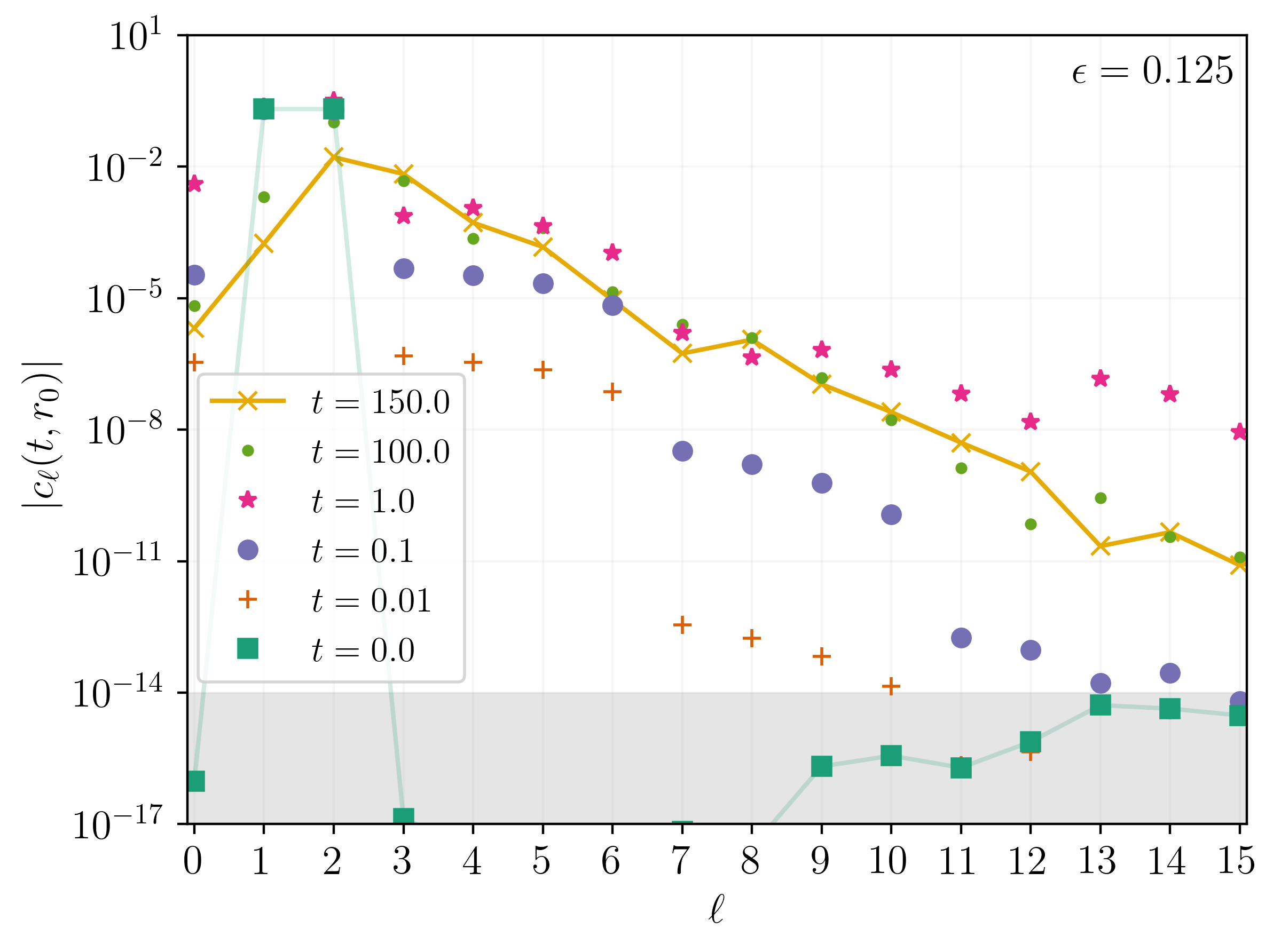
Figure 14: The $\ell$-spectrum of the solutions for $\epsilon=0.25$ (left panel) and $\epsilon=0.125$ (right panel) at different times in the evolution, as captured by the Fourier coefficients (18), with a logarithmic scale on the vertical axis. Lines joining the points for the times $t=0$ and $t=150$ have been added to guide the reader. The grey shading indicates where the numerical floor of our simulations is.

In contrast with the $\epsilon=1$-case of Section VI.3, we do not observe any growth of second derivatives of our numerical solutions for $\epsilon=0.25$ and $\epsilon=0.125$ within the time interval evolved. We argue that the absence of growth may be ascribed to the decreased efficiency of the angular-mode cascade: If the growth of second derivatives eventually occurs, it would become manifest over a longer interval of time than the one for which we can numerically evolve. Nonetheless, we expect sufficiently high-order derivatives (as well as sufficiently high-order energies) of the solutions to manifestly grow already over the time interval considered in this work. With the fourth-order finite difference methods we employ, computation of high-order derivatives becomes problematic in terms of the resolution that would be needed for accurate results, and so we leave to future investigations a thorough study of high-order quantities for small values of $\epsilon$, and in particular their potential growth.

VII Discussion and outlook

In this work, we have studied numerical solutions to the cubic (defocusing) wave equation (16) on a model geometry possessing stably trapped null geodesics. We have shown that initial data which are axisymmetric, radially localised within the stable trapping region, and supported on a small number of low-order multipole modes give rise to solutions whose high-order derivatives grow in time. The growth occurs within the stable trapping region and is induced by a direct angular-mode cascade, with higher-order modes being excited by the nonlinear interactions and eventually dominating the low-modes in the evolution. Moreover, we argued that the turbulent behavior of such solutions may persist for small (amplitude) initial data of the form considered.

The growth of high-order derivatives hints at the possibility that higher-order quantities of our numerical solutions fail to remain uniformly bounded in time. In particular, with reference to the growth of second-order derivatives of Figures 5 and 6, there may not exist a uniform bound for the second-order energy $\mathbb{E}^{2}[\phi](t)$ of the numerical solution in terms of its initial second-order energy $\mathbb{E}^{2}[\phi](0)$ (cf. inequality (13) for $k=2$ in Theorem 1 for linear waves). The failure of uniform boundedness may originate from either an arbitrarily large (but finite) growth or an unbounded growth of the quantity $\mathbb{E}^{2}[\phi](t)$, and would be in stark contrast with known (mathematically rigorous) results on the decay of higher-order quantities for solutions to equation (16) on asymptotically flat spacetimes with unstable trapping (e.g., on Schwarzschild exterior spacetimes). The uniform boundedness and, more generally, the asymptotic dynamics of our numerical solutions are left for future investigations.

In the following, we consider some open questions and further elaborate on our numerical results in connection with the existing literature.

VII.1 Scalar turbulence and stable trapping beyond our model

Based on the nature of the turbulent mechanism observed, we speculate on three aspects of our model problem which go beyond the numerical results presented in this work:

• Generic initial data for equation (16) on our model spacetime. For equation (16) on our model spacetime, the turbulent dynamics may arise for generic smooth, compactly supported initial data (without any symmetry assumption). For initial data radially supported away from the stable trapping region, one expects that part of the solution would always reach and propagate into the effective potential well and trigger the turbulent evolution. See Sections VI.2 and VI.4 for some considerations on the persistence of the turbulent dynamics for initial data which are different from the ones considered in this work.

• Other nonlinear wave equations on our model spacetime. The present work considers numerical solutions to a single nonlinear wave equation. Nonetheless, one would expect that the turbulent mechanism does not rely on the precise structure of the nonlinearity, and thus the slow linear decay may lead to a turbulent dynamics of solutions to a large class of nonlinear wave equations on our model spacetime. The class may, in particular, include wave equations with derivative nonlinearities of the form (3).

• Equation (16) on general spacetimes with stable trapping. The turbulent dynamics of solutions to equation (16) may occur for more general spacetimes possessing stably trapped null geodesics, meaning that the presence of stable trapping alone may suffice to induce slow linear decay and the turbulent behaviour of nonlinear solutions. These more general spacetimes may be possibly characterised by different asymptotic structures, symmetries or number of dimensions from our model spacetime, or possess additional structures like an event horizon. Examples of such spacetimes may include the ones considered in [13, 14, 9, 15].

VII.2 Turbulent gravitational waves

Whether turbulence (generically) persists for small gravitational perturbations of our motivating spacetimes (i.e., ultracompact objects and black strings), and how it would affect their global dynamics, are questions which remain open. Nonetheless, there are two primary features of the scalar turbulent dynamics in our model problem which we argue already imply that the possible gravitational turbulent dynamics, though likely leading to a similar turbulent cascade in the spectrum of partially trapped gravitational waves, would not have any dire consequences for the evolution of the corresponding spacetimes. First, the physical energy density of scalar waves, i.e., the (first-order) energy density of our numerical solutions, does not grow with time. Second, the effective potential barrier generating the stable trapping of scalar waves has finite height, and hence the (first-order) energy within the trapping region of initially trapped waves decays with time, albeit slowly. Moreover, we note that the direct cascade to arbitrarily small length-scales would not a-priori constitute an obstruction to considering the global gravitational turbulent dynamics of these spacetimes within the regime of classical general relativity. Indeed, where the classical regime fails as a theory predicting the structure of spacetime, and would need a theory of “quantum gravity” to take over, is when singularities (clothed or not) or Cauchy horizons form, neither of which is length-scale dependent in general relativity.

Beyond this, one can only speculate on the global dynamics of the possible gravitational turbulent dynamics, in that our model problem does not capture the back-reaction of partially trapped gravitational perturbations on the spacetime. In the following paragraphs, we discuss some lines of speculation in this direction.

Suppose that a gravitational perturbation is initially localised within a stable trapping volume of characteristic size $R$ and its (first-order) energy is initially small. For such a perturbation, the energy within the stable trapping volume will remain small during evolution, meaning that the average back-reaction over the trapping volume induced by the perturbation will remain small over time. While the average back-reaction remains small, the turbulent dynamics drives a direct energy cascade transferring part of the energy of the perturbation to progressively smaller wavelengths $\lambda$. In particular, one could envision a late-time state where part (or perhaps most) of the energy transfers to modes with very small characteristic wavelengths $\lambda\ll R$, raising the question of whether a black hole of radius of order $\lambda$ could form. Since the energy of the perturbation within the trapping volume remains small at all scales and no manifest focusing mechanism of the perturbation appears to be present, we argue that this would be very unlikely. Indeed, by hoop conjecture arguments, for a hyperspherical black hole of radius of order $\lambda$ to form, the energy density of the perturbation within the corresponding volume would need to be of order $\lambda^{-2}$ (and thus be very large for a black hole to form at very small scales). Reaching such a density would require a “rogue wave” : a constructive superposition of waves at a location resulting in an anomalously large amplitude, hence energy density there. The formation of rogue waves has been observed as a rare phenomenon in various wave and dispersive systems in physics, one notable example being the propagation of light in a reflective optical fiber [46]. However, in our dynamics it appears unlikely that this type of rare phenomenon may generically lead to gravitational collapse. This is both because of the continuous transfer of energy to progressively smaller scales within the direct turbulent cascade, and that the effective confinement due to stable trapping is only partial, implying that the probability of black hole formation from such superpositions at any given scale decreases with time. In the case of black strings, we remark that, even if the turbulent dynamics were to lead to a small black hole forming within the trapping region at some intermediate time, one would expect that the small black hole will eventually merge with the central horizon, thus not affecting the nature of the end state of the dynamics.

We point out that, as opposed to complete dispersion, there may exist end states where a finite amount of energy remains within the trapping region, i.e., a kind of gravitational geon which condenses outside the central object. However, we would expect the eventual dispersion of the initially trapped, small gravitational perturbation as the generic end state of the global dynamics.

We observe that two factors, if they occur for our motivating spacetimes, could alter the picture described above:

• Rotating black strings. If the spacetime is a rotating black string, the angular momentum of the spacetime is a potential source of energy to feed the turbulent dynamics of a trapped gravitational perturbation. Nonetheless, in view of the arguments already discussed, we argue that the additional source of energy would still unlikely lead to black hole formation through the turbulent cascade. On the other hand, rotating black strings are known to suffer from a superradiant instability [47], which would likely dominate the global dynamics of these spacetimes.

• Ultracompact objects for certain matter models. Different considerations may apply to ultracompact objects when governed by nonlinear matter fields which undergo a similar turbulent dynamics (to the one described in vacuum) within the region of stable trapping (and for which other nonlinear dissipative mechanisms, such as viscosity in a fluid, are not strong enough to limit or halt the turbulent cascade). In particular, since the outer region of the central object in such spacetimes must necessarily be within the region of stable trapping, the central object may possibly provide a source of energy to feed the turbulent dynamics of trapped matter perturbations. Similar considerations to those above suggest it is unlikely that a large enough “rogue” matter wave could form in the trapped region to lead to small black hole formation there. Instead, for star-like compact objects, what could significantly affect the dynamics of the system comes from the transfer of energy from the core to the region of stable trapping, driven by the turbulent cascade in the latter. This would lead to an effective migration of the core along the star’s mass-radius curve, with the two likely outcomes being either the star migrates to a larger, less dense configuration without a stable trapping region, or it evolves the opposite way and collapses to a black hole (see [48] for similar conjectures on the endstate, as well as how the presence of an ergoregion may influence the dynamics). These outcomes are consistent with what was shown to occur in numerical simulations of two classes of ultracompact bosonic stars in [49]. For shell-like ultracompact objects (such as AdS black bubbles or gravastars), the matter present in the spacetime is confined to the shell region, and thus the turbulent dynamics would not be expected to significantly change the overall properties of the shell (especially if the shell material is viscous). The relevant questions on the global dynamics of these latter objects would then revert to those for partially trapped gravitational perturbations.

VII.3 Related works on turbulence

Wave turbulence is a classical theme in the analysis of model equations from physics [50, 51]. Nonlinear models for which the existence of turbulent solutions has been widely studied include examples of nonlinear dispersive equations on compact domains, such as the nonlinear Schrödinger equation on the torus [52, 53] and the nonlinear Szëgo equation on the circle [54].

In the realm of general relativity, turbulence due to perfect confinement arises in the nonlinear dynamics of Anti-de Sitter (AdS) space, when reflective boundary conditions are imposed at the conformal boundary. The numerical work [56] shows the nonlinear instability of AdS space as a solution to the Einstein–scalar field system (with negative cosmological constant) in spherical symmetry (see also the related works [57, 58]): There exist arbitrarily small perturbations which exhibit a turbulent dynamics leading to the formation of a black hole in finite time. More recently, works [61, 62] have given a first rigorous proof of instability of AdS space as a solution to the Einstein–null dust and Einstein–massless Vlasov systems (with negative cosmological constant) in spherical symmetry, in which turbulence is again the driving mechanism leading to black hole formation. Without any symmetry assumption, works [63, 64] and [65] have independently conjectured that AdS space remains nonlinearly unstable (to black hole formation) as a solution to the vacuum Einstein equations (with negative cosmological constant). The mathematically rigorous resolution of the conjecture remains a major open problem in the subject (see [66, 67, 68] for some numerical investigations).

The dynamics of asymptotically AdS black holes with reflective boundary conditions may also exhibit some turbulent behaviour. Indeed, linear waves on Schwarzschild–AdS and Kerr–AdS black hole exteriors (the latter satisfying the so-called Hawking–Reall bound) only decay sharp-logarithmically in time [69, 13], due to the presence of stable trapping. For linearised gravitational perturbations, one thus expects these spacetimes to be only weakly stable (see [70] and [71, 72, 73] for rigorous results in this direction). The nonlinear (both scalar and gravitational) dynamics of these spacetimes remains, for the most part, to be understood. Based on the numerical result presented in this work and in line with what discussed for the expected dynamics of our motivating spacetimes, one may speculate that these spacetimes similarly suffer from a turbulent (scalar and gravitational vacuum) dynamics. Examples of turbulent black holes already appear, and have been numerically investigated, in different scenarios [78, 79].

Appendix A Initial data and angular modes

In this appendix, we consider initial data for equation (16) of the form

$$\phi|_{t=0} =\frac{1}{\mathbb{E}_{\text{nl}}[\hat{\phi}](0)}\underbrace{\left(\epsilon\,u(r)\cdot\sum_{\left[\ell\right]}\ell^{-1}Y_{0}^{\ell}(\vartheta)\right)}_{:=\hat{\phi}}\,, \partial_{t}\phi|_{t=0} =0\,,$$ (33)

with the choices

$$\epsilon =1\,, r_{0,1} =0.02\,, r_{0,2} =0.6$$

and

$$u(r)=4000\cdot\frac{\left(r-r_{0,1}\right)^{4}\left(r-r_{0,2}\right)^{4}}{\left(r_{0,1}-r_{0,2}\right)^{8}}$$

for $r\in[r_{0,1},r_{0,2}]$ and identically vanishing otherwise. Up to the rescaling by the initial energy $\mathbb{E}_{\text{nl}}[\hat{\phi}](0)$ and by the factors $\ell^{-1}$, the initial data (33) are of the same form as the initial data (27) considered in Sections VI.3 and VI.4.

The aim of this appendix is to compare the numerical evolutions of the initial data (33) for different choices of $[\ell]$. The additional rescalings in (33) are introduced so that, for any choice of $[\ell]$, the initial data possess the same energy (i.e., $\mathbb{E}_{\text{nl}}[\phi](0)=1$), which is moreover (approximately) equidistributed among the $\ell$-angular modes contained in the initial data. In our comparative analysis, this will be convenient for isolating properties of the solution which only depend on the choice of $[\ell]$.

In Figure 15, we examine the time evolution of the $\ell$-spectrum of the numerical solutions for different choices of $[\ell]$. As for the case $[\ell]=[1,2]$ analysed in Figure 11, one can see consecutive generations of angular modes getting excited in the evolution. Which excited modes are included in the first generation depends on the choice of $[\ell]$. Moreover, we note that single-mode initial data with higher $\ell$ yields a first generation of excited modes which is more populated (compare the first panel for $[\ell]=[1]$ with the fourth panel for $[\ell]=[4]$ in the figure). For two-mode initial data, the combination of an odd mode with an even mode yields a more populated first generation of excited modes than an odd-odd combination (compare the fifth panel for $[\ell]=[1,2]$ with the sixth panel for $[\ell]=[1,3]$ in the figure). Richer initial mode-configurations lead to more populated first generations of excited modes (see seventh and eight panel). We also note that single-odd-mode (single-even-mode) initial data and odd-odd (even-even) two-mode initial data only excite odd (even and $\ell=0$) modes.

The $\ell$-spectrum of the cubic power of the solution $\phi^{3}$ at the initial time is supported on a range of angular modes which depends on the choice of $[\ell]$ (see Figure 16, to be compared with Figure 10). The $\ell$-spectra of Figure 16 drive the corresponding first generations of excited modes of Figure 15. In agreement with what is observed in Figure 15, the $\ell$-spectrum in Figure 16 is richer for higher (rather than lower) single-mode initial data, for odd-even (rather than odd-odd) two-mode initial data and for multiple-mode (rather than single or two-mode) initial data. One can also read-off the parity of the excited modes described in Figure 15.

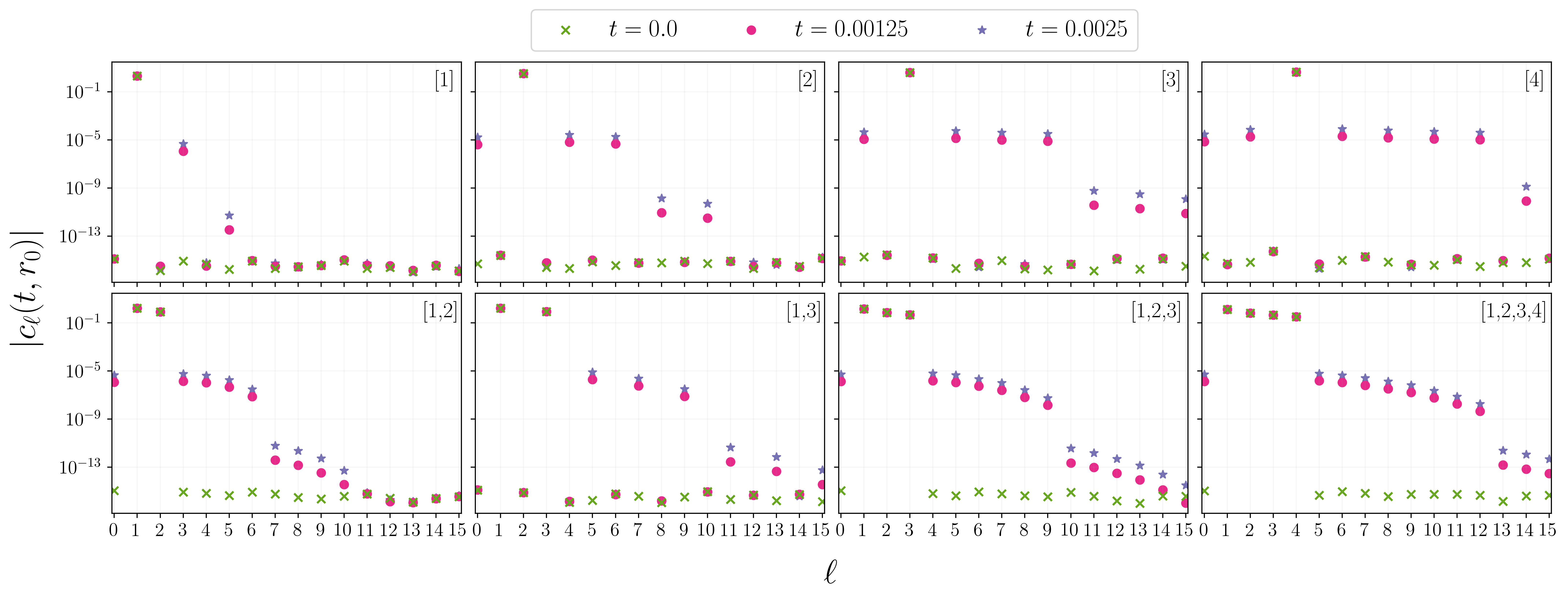
Figure 15: The $\ell$-spectrum of the solution at different times in the evolution, as captured by the Fourier coefficients (18), with a logarithmic scale on the vertical axis. Each panel corresponds to the choice of $[\ell]$ indicated in the top-right corner of the panel. The lowest value on the vertical axis corresponds to the numerical floor of our simulation. The top panels show initial data supported on a single angular mode, whereas the bottom panels show initial data supported on different combinations of angular modes. We note that the evolution times considered in the figure are much shorter than the ones in Figure 11.

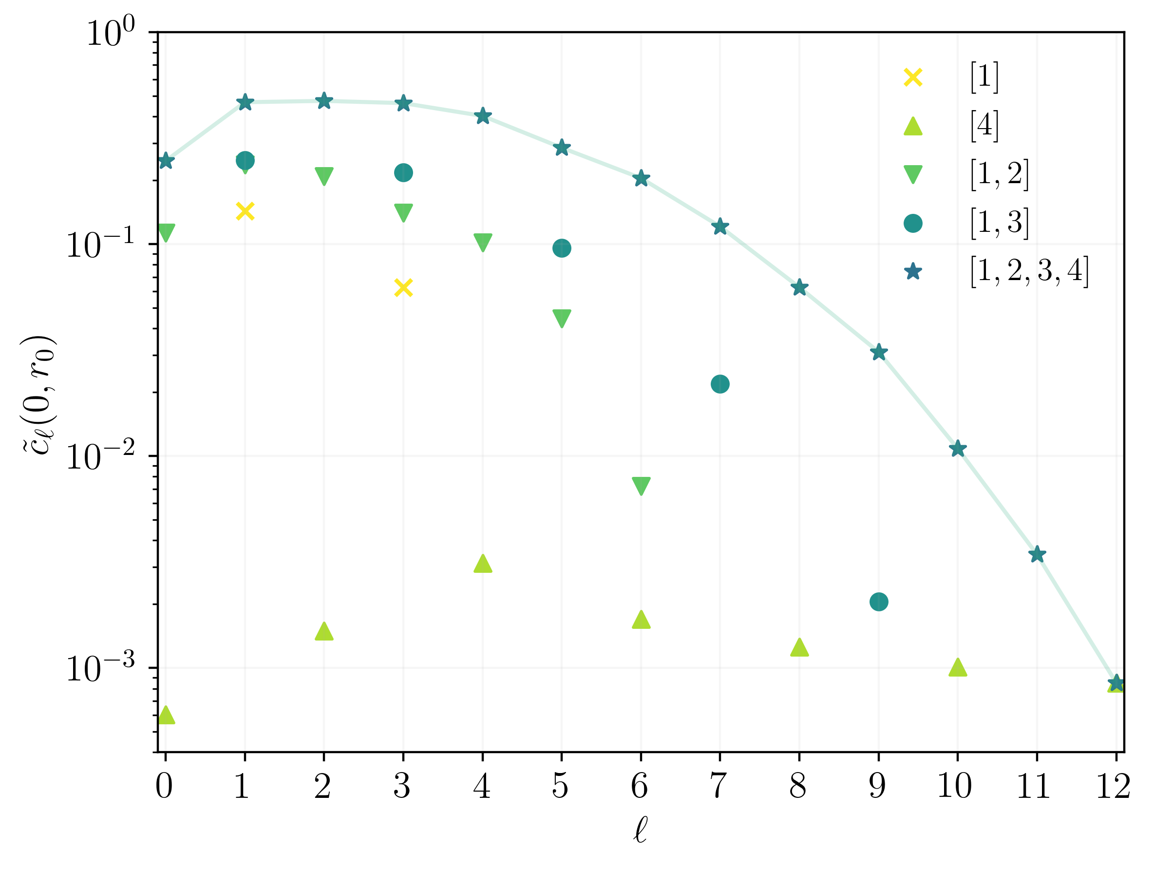
Figure 16: The $\ell$-spectrum of the cubic power $\phi^{3}$ of the solution at the initial time, as captured by the Fourier coefficients (19), with a logarithmic scale on the vertical axis. The range of the vertical axis is so as to include all the non-trivial values for the Fourier coefficients considered (i.e., no points appear between the lower end of the axis and the numerical floor of our simulation, cf. Figure 10). Each set of points corresponds to the initial data (33) for the choice of $[\ell]$ indicated in the top-right corner of the panel. A line joining the points for the case $[\ell]=\left[1,2,3,4\right]$ has been added to guide the reader. We note that the Fourier coefficients plotted are all positive, with no absolute value applied to the Fourier coefficients on the vertical axis.

Appendix B Convergence tests

Let $h$ be a grid function from three levels of increasing resolutions $h^{\textrm{low}}$, $h^{\textrm{mid}}$ and $h^{\textrm{high}}$. We test the convergence of our numerical simulations by computing the convergence factor

$$Q_{h}(t)=\frac{1}{\ln 2}\ln\left(\frac{\left\lVert h^{\textrm{mid}}-h^{\textrm{low}}\right\rVert_{\ell^{2}}(t)}{\left\lVert h^{\textrm{high}}-h^{\textrm{mid}}\right\rVert_{\ell^{2}}(t)}\right)\,,$$ (34)

where the grid spacing of the coarsest resolution is $(\Delta_{Y},\Delta_{Z})=(\Delta^{\textrm{low}}_{Y},\Delta^{\textrm{low}}_{Z})$ and is decreased by a factor of $2$ for subsequent higher resolutions (e.g., $\Delta_{Y}^{\rm high}=\,\Delta^{\rm mid}_{Y}/2=\,\Delta^{\rm low}_{Y}/4$). For all our simulations, we have set the Courant factor to $C=0.5$ (i.e., $\Delta_{t}=0.5\,\Delta_{Y}$) and applied a sixth-order Kreiss–Oliger dissipation, with $\epsilon_{\rm KO}=0.3$.

Figures 17 and 18 show the time evolution of the convergence factor $Q_{\phi}(t)$ for the numerical solution to equation (16) arising from the initial data analysed in Sections VI.3 and VI.4. Analogously, Figures 19 and 20 show the values of the quantities (30) and (31) respectively, for three increasing resolutions, illustrating how small the numerical error is for these quantities. Different choices of $\epsilon$ for the amplitude of the initial data are considered. For $\epsilon=1$, Figure 18 also plots the time evolution of the convergence factor for the linear solution to equation (10). The resolution adopted for the numerical simulations is $(\Delta^{\textrm{low}}_{Y},\Delta^{\textrm{low}}_{Z})=(0.00125,0.00125)$, meaning that, for the highest resolution $(\Delta^{\textrm{high}}_{Y},\Delta^{\textrm{high}}_{Z})$, we evolve a grid size of $3201\times 6401$. From Figure 17, one sees that, at early times, the convergence factor is lower than fourth-order, with approximately third-order convergence at time $t=3$. Nonetheless, Figure 18 shows that, by time $t=25$, we achieve approximately fourth-order convergence (recall that our numerical scheme is indeed forth-order, see Section V) for the cases $\epsilon=\{0.75,1,1.25\}$ (which are the ones analysed in Sections VI.3 and VI.4). We remark that, in particular, Figure 18 exhibits approximately fourth-order convergence over the time interval for which the growth of second-order derivatives of the numerical solutions is observed in Section VI.3.

We test the convergence of the time evolution of the energy (17) of the numerical solution arising from the initial data analysed in Sections VI.3 and VI.4 (with $\epsilon=1$). For the sake of the convergence test, the energy (17) is computed over $75\%$ of the computational domain (i.e., $X=0$, $Y\in\left[0,0.75\right]$ and $Z\in\left[-0.75,0.75\right]$), so as to exclude the relatively large numerical loss of energy coming from dissipation of outgoing waves as they become under-resolved propagating into the volume where the effects of spatial compactification dominate (i.e., we are restricting the domain of integration to a region which is well resolved in our compactified coordinates (25)). See Figure 21.

Lastly, Figure 22 shows convergence for the Fourier coefficients of the numerical solution arising from the initial data analysed in Section VI.4 (with $\epsilon=1$). For visualization purposes, we are only showing the convergence at two times ($t=50$ and $t=150$, the latter being the largest time we run) for all the coefficients. We have also tested the convergence for the lower amplitude cases, which are numerically less challenging.

Figure 17: The evolution of the convergence factor (34) over the time interval $t\in[0,3]$ for the numerical solutions analysed in Figure 3.

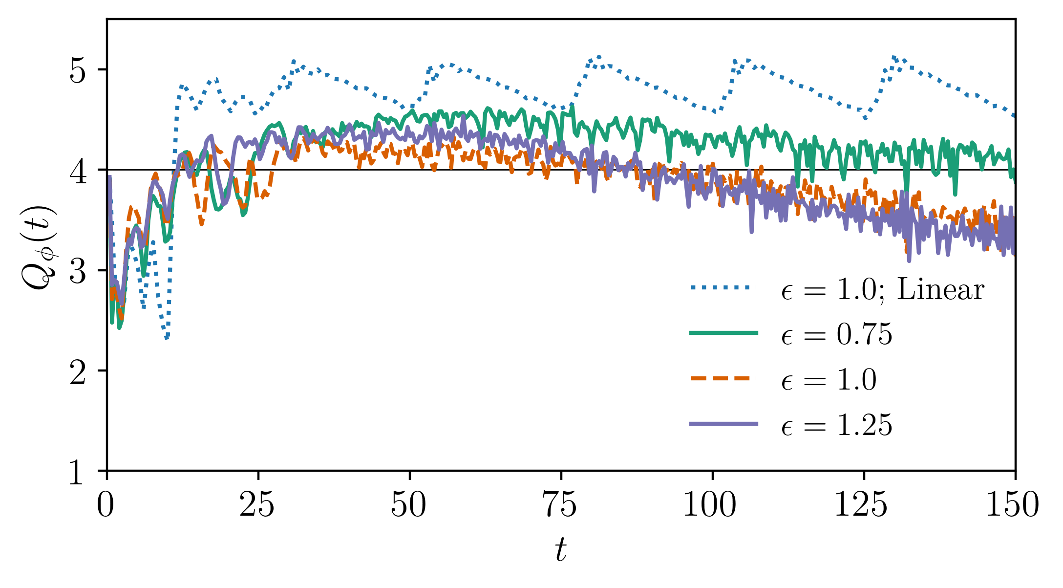
Figure 18: The evolution of the convergence factor (34) over the time interval $t\in[0,150]$ for the numerical solutions analysed in Figures 4, 5, 6, 7, 8 and 9.

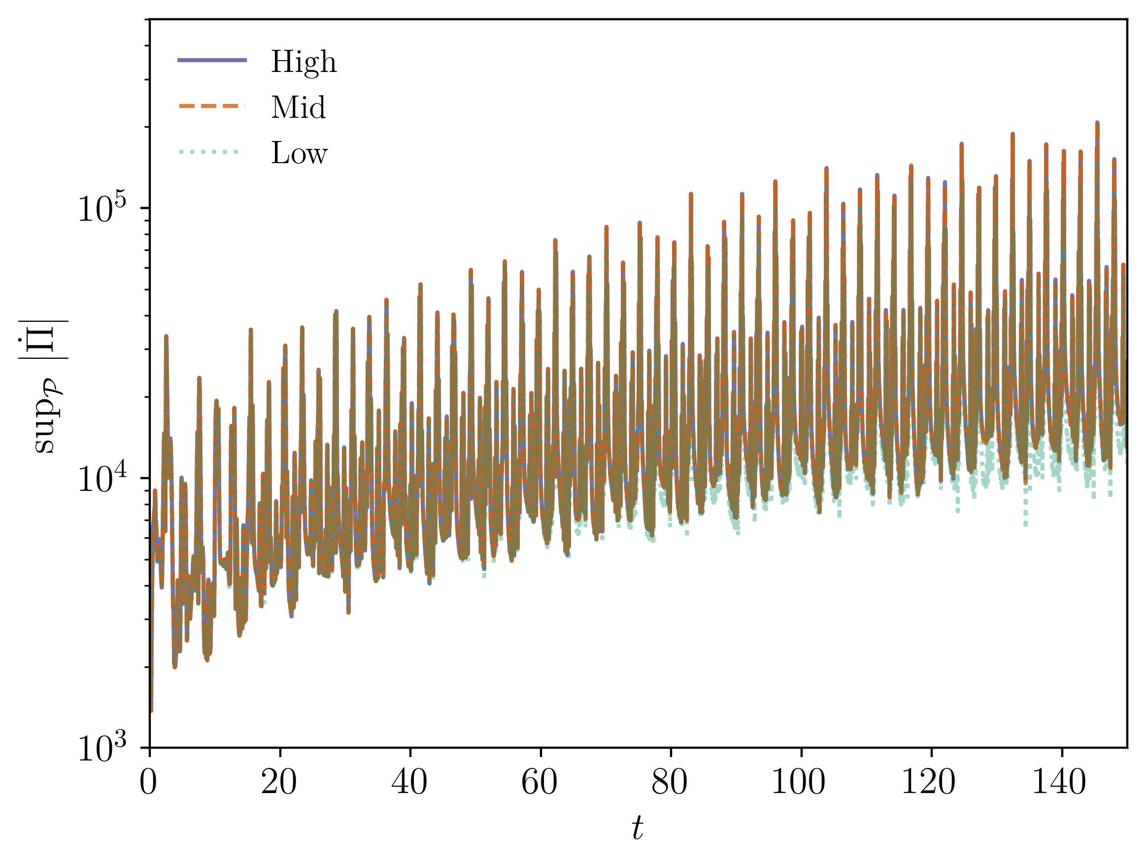
Figure 19: The evolution of the quantity (30) over the time interval $t\in[0,150]$ for $\epsilon=1$ at three different (increasing by a factor of two) resolutions, starting with $(\Delta^{\rm low}_{Y},\Delta^{\rm low}_{Z})=(0.00125,0.00125)$. The numerical error in this quantity is very small. At $t=150$, for example, the relative error computed using the Mid and High resolutions is about $0.58\%$.

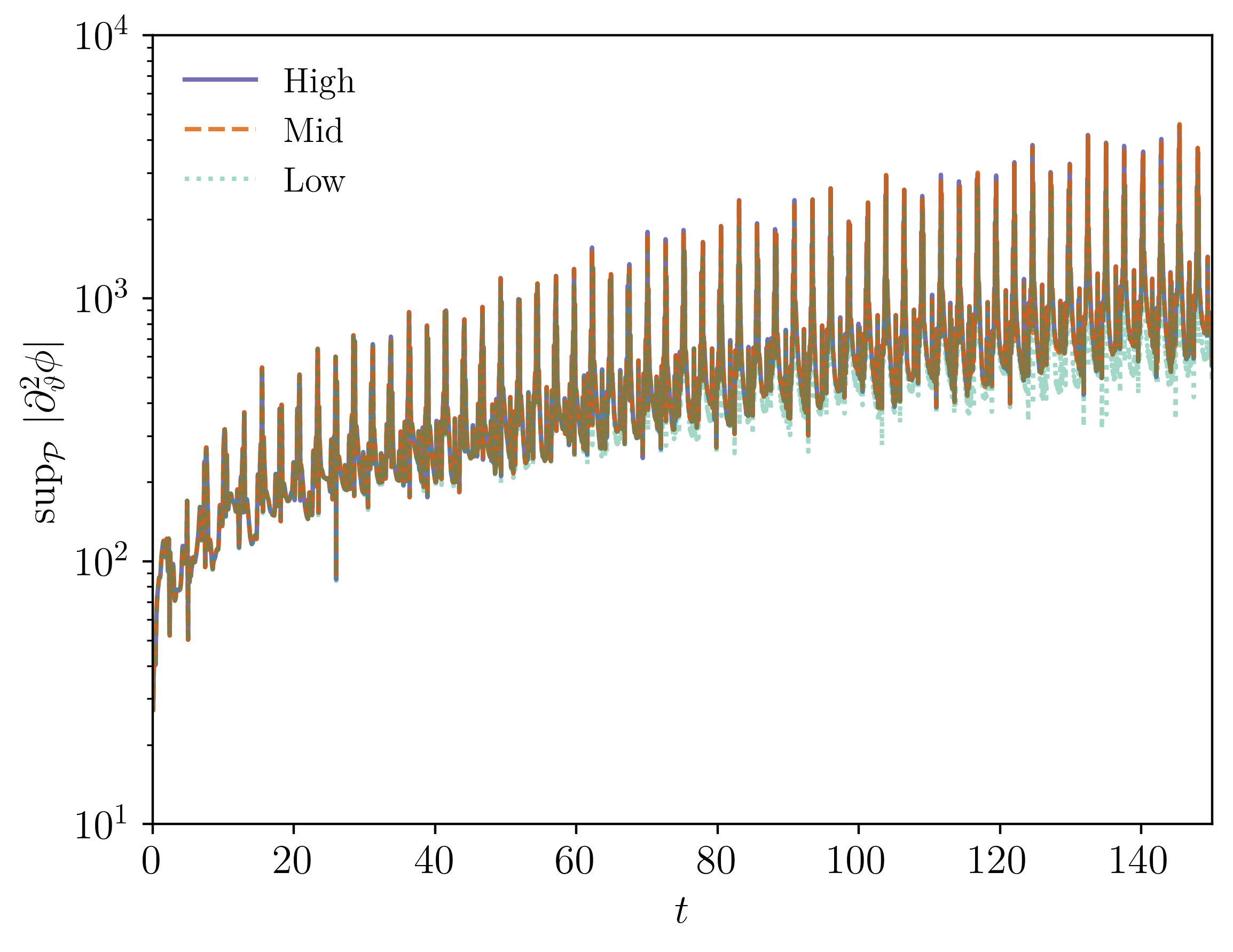
Figure 20: The evolution of the quantity (31) over the time interval $t\in[0,150]$ for $\epsilon=1$ at three different (increasing by a factor of two) resolutions, starting with $(\Delta^{\rm low}_{Y},\Delta^{\rm low}_{Z})=(0.00125,0.00125)$.The numerical error in this quantity is very small. At $t=150$, for example, the relative error computed from the Mid and High resolutions is about $0.55\%$.

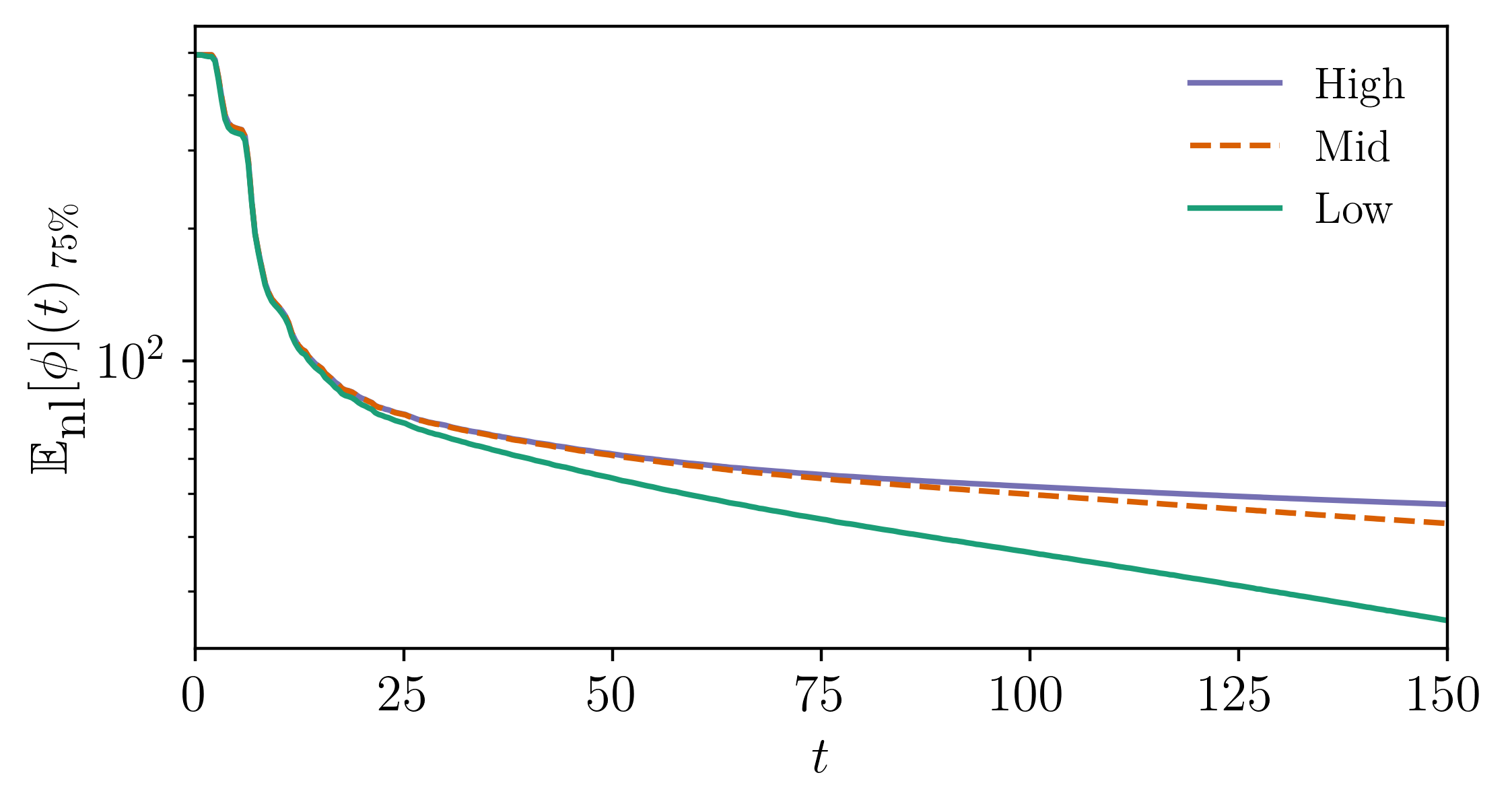
Figure 21: The evolution of the energy (17) over the time interval $t\in[0,150]$ for the numerical solutions analysed in Figures 4, 5 and 6. The energy is computed over $75\%$ of the computational domain centered about the origin, for three resolutions. The resolution is increasing by factors of $2$, starting with the lowest resolution given by $(\Delta^{\rm low}_{Y},\Delta^{\rm low}_{Z})=(0.00125,0.00125)$. The energy decreases over time as it leaks out of the central volume to which we limit its calculation (recall that the energy (17) is conserved over time if computed over $100\%$ of the computational domain).

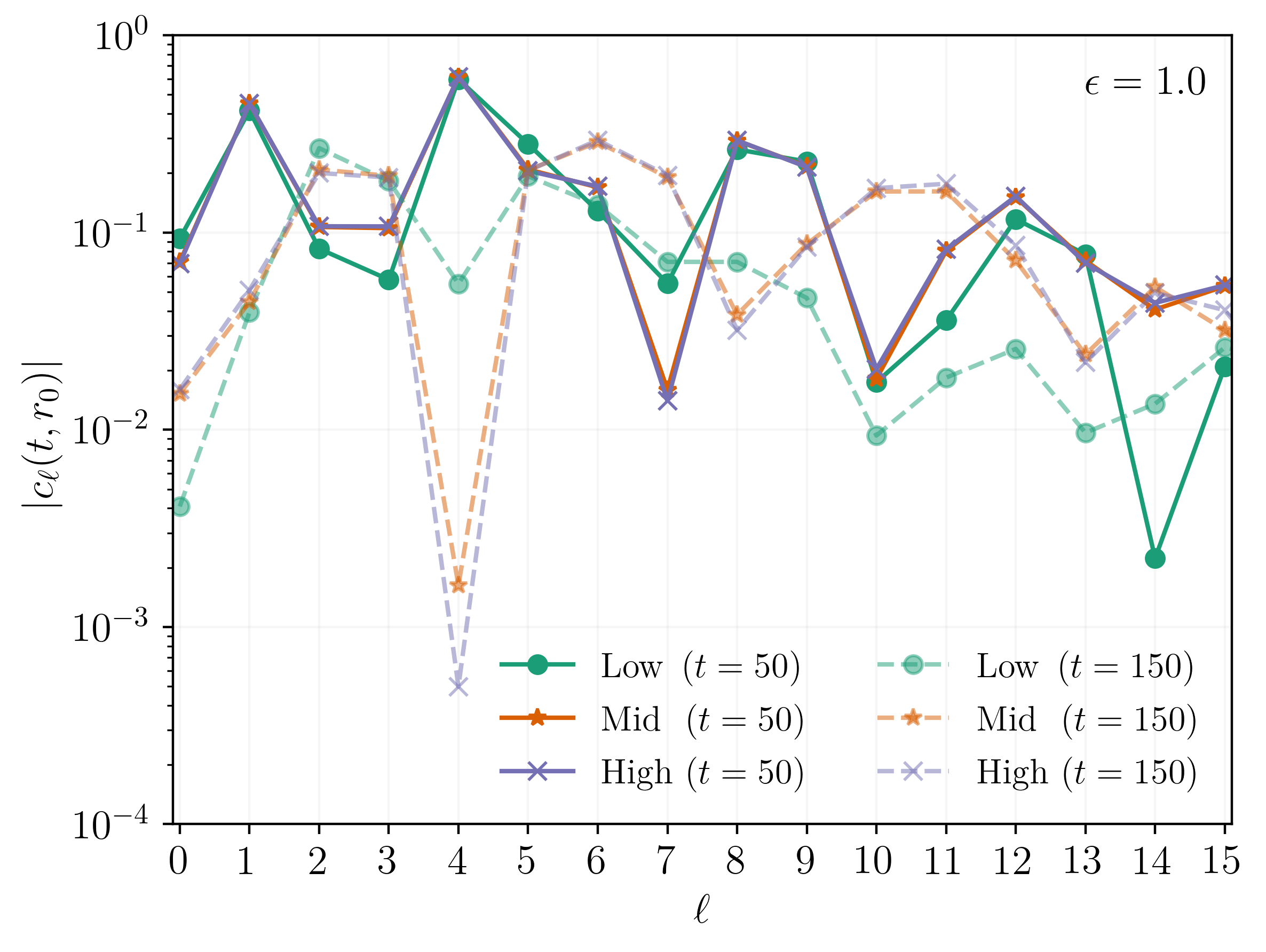
Figure 22: The $\ell$-spectrum of the numerical solution analysed in Figures 11 and 12 at two different times in the evolution. The times considered are $t=50$ (dark solid lines) and $t=150$ (shaded dashed lines). Three increasing resolutions are plotted, starting with $(\Delta^{\rm low}_{Y},\Delta^{\rm low}_{Z})=(0.00125,0.00125)$. Analogous convergence has been tested for the numerical solutions analysed in Figure 14, which are computationally less challenging than the higher-amplitude case shown in this figure.

References

- Courant and Hilbert [1953] R. Courant and D. Hilbert, Methods of Mathematical Physics: Partial differential equations, Methods of Mathematical Physics (Interscience Publishers, 1953).
- Ruffini and Bonazzola [1969] R. Ruffini and S. Bonazzola, Systems of selfgravitating particles in general relativity and the concept of an equation of state, Phys. Rev. 187, 1767 (1969).
- Colpi et al. [1986] M. Colpi, S. L. Shapiro, and I. Wasserman, Boson Stars: Gravitational Equilibria of Selfinteracting Scalar Fields, Phys. Rev. Lett. 57, 2485 (1986).
- Danielsson et al. [2017] U. H. Danielsson, G. Dibitetto, and S. Giri, Black holes as bubbles of AdS, JHEP 10, 171, arXiv:1705.10172 [hep-th] .
- Mathur [2005] S. D. Mathur, The Fuzzball proposal for black holes: An Elementary review, Fortsch. Phys. 53, 793 (2005), arXiv:hep-th/0502050 .
- Mazur and Mottola [2004] P. O. Mazur and E. Mottola, Gravitational vacuum condensate stars, Proc. Nat. Acad. Sci. 101, 9545 (2004), arXiv:gr-qc/0407075 .
- Cardoso and Pani [2019] V. Cardoso and P. Pani, Testing the nature of dark compact objects: a status report, Living Rev. Rel. 22, 4 (2019), arXiv:1904.05363 [gr-qc] .
- Benomio [2020] G. Benomio, The wave equation on black rings and the linear stability of slowly rotating Kerr spacetimes, PhD thesis, Imperial College London (2020).
- Benomio [2021] G. Benomio, The stable trapping phenomenon for black strings and black rings and its obstructions on the decay of linear waves, Anal. Part. Diff. Eq. 14, 2427 (2021), arXiv:1809.07795 [gr-qc] .
- Gregory and Laflamme [1993] R. Gregory and R. Laflamme, Black strings and p-branes are unstable, Phys. Rev. Lett. 70, 2837 (1993), arXiv:hep-th/9301052 .
- Dafermos et al. [2016] M. Dafermos, I. Rodnianski, and Y. Shlapentokh-Rothman, Decay for solutions of the wave equation on Kerr exterior spacetimes III: The full subextremal case , Ann. of Math. (2) 183, 787 (2016).
- Dyatlov [2011] S. Dyatlov, Quasi-normal modes and exponential energy decay for the Kerr-de Sitter black hole, Commun. Math. Phys. 306, 119 (2011), arXiv:1003.6128 [math.AP] .
- Holzegel and Smulevici [2014] G. Holzegel and J. Smulevici, Quasimodes and a lower bound on the uniform energy decay rate for Kerr-AdS spacetimes, Anal. PDE 7, 1057 (2014).
- Keir [2016] J. Keir, Slowly decaying waves on spherically symmetric spacetimes and ultracompact neutron stars, Classical Quantum Gravity 33, 135009, 42 (2016).
- Gunasekaran and Kunduri [2021] S. Gunasekaran and H. K. Kunduri, Slow decay of waves in gravitational solitons, Annales Henri Poincare 22, 821 (2021), arXiv:2007.04283 [gr-qc] .
- Keir [2019] J. Keir, Wave propagation on microstate geometries, Annales Henri Poincare 21, 705 (2019), arXiv:1609.01733 [gr-qc] .
- Idelon-Riton [2016] G. Idelon-Riton, Quasimodes and a lower bound for the local energy decay of the Dirac equation in Schwarzschild-Anti-de Sitter spacetime, ArXiv e-prints (2016), arXiv:1610.05542 [math-ph] .
- Luk [2013] J. Luk, The null condition and global existence for nonlinear wave equations on slowly rotating Kerr spacetimes, J. Eur. Math. Soc. (JEMS) 15, 1629 (2013).
- Dafermos et al. [2024] M. Dafermos, G. Holzegel, I. Rodnianski, and M. Taylor, Quasilinear wave equations on Kerr black holes in the full subextremal range , (2024), arXiv:2410.03639 [gr-qc] .
- Hintz and Vasy [2016] P. Hintz and A. Vasy, Global analysis of quasilinear wave equations on asymptotically Kerr-de Sitter spaces, Int. Math. Res. Not. 2016, 5355 (2016), arXiv:1404.1348 [math.AP] .
- Klainerman [1986] S. Klainerman, The null condition and global existence to nonlinear wave equations, in Nonlinear systems of partial differential equations in applied mathematics, Part 1 (Santa Fe, N.M., 1984), Lectures in Appl. Math., Vol. 23 (Amer. Math. Soc., Providence, RI, 1986) pp. 293–326.
- Christodoulou [1986] D. Christodoulou, Global solutions of nonlinear hyperbolic equations for small initial data, Comm. Pure Appl. Math. 39, 267 (1986).
- John [1981] F. John, Blow-up for quasi-linear wave equations in three space dimensions, Communications on Pure and Applied Mathematics 34, 29 (1981), https://onlinelibrary.wiley.com/doi/pdf/10.1002/cpa.3160340103 .
- Dafermos et al. [2021] M. Dafermos, G. Holzegel, I. Rodnianski, and M. Taylor, The nonlinear stability of the Schwarzschild family of black holes, arXiv e-print 2104.08222 (2021).
- Klainerman and Szeftel [2023] S. Klainerman and J. Szeftel, Kerr stability for small angular momentum, Pure and Applied Mathematics Quarterly 19 (2023).
- Hintz and Vasy [2018] P. Hintz and A. Vasy, The global non-linear stability of the Kerr–de Sitter family of black holes, Acta Math. 220, 1 (2018).
- Bachelot and Nicolas [1993] A. Bachelot and J.-P. Nicolas, équation non linéaire de Klein-Gordon dans des métriques de type Schwarzschild, C. R. Acad. Sci. Paris Sér. I Math. 316, 1047 (1993).
- Nicolas [1995] J.-P. Nicolas, Nonlinear Klein-Gordon equation on Schwarzschild-like metrics, J. Math. Pures Appl. (9) 74, 35 (1995).
- Blue and Soffer [2007] P. Blue and A. Soffer, A space-time integral estimate for a large data semi-linear wave equation on the Schwarzschild manifold, Lett. Math. Phys. 81, 227 (2007).
- Blue and Soffer [2003] P. Blue and A. Soffer, Semilinear wave equations on the Schwarzschild manifold. 1. Local decay estimates, Adv. Diff. Eq. 8, 595 (2003), arXiv:gr-qc/0310091 .
- Horowitz and Strominger [1991] G. T. Horowitz and A. Strominger, Black strings and P-branes, Nucl. Phys. B 360, 197 (1991).
- Collingbourne [2021] S. C. Collingbourne, The Gregory–Laflamme instability of the Schwarzschild black string exterior, J. Math. Phys. 62, 032502 (2021), arXiv:2007.08441 [gr-qc] .
- Gubser and Mitra [2002] S. S. Gubser and I. Mitra, Instability of charged black holes in Anti-de Sitter space, Clay Math. Proc. 1, 221 (2002), arXiv:hep-th/0009126 .
- Gubser and Mitra [2001] S. S. Gubser and I. Mitra, The Evolution of unstable black holes in anti-de Sitter space, JHEP 08, 018, arXiv:hep-th/0011127 .
- Hovdebo and Myers [2006] J. L. Hovdebo and R. C. Myers, Black rings, boosted strings and Gregory-Laflamme, Phys. Rev. D73, 084013 (2006), arXiv:hep-th/0601079 [hep-th] .
- Reall [2001] H. S. Reall, Classical and thermodynamic stability of black branes, Phys. Rev. D 64, 044005 (2001), arXiv:hep-th/0104071 .
- Figueras et al. [2011] P. Figueras, K. Murata, and H. S. Reall, Black hole instabilities and local Penrose inequalities, Class. Quant. Grav. 28, 225030 (2011), arXiv:1107.5785 [gr-qc] .
- Hollands and Wald [2013] S. Hollands and R. M. Wald, Stability of Black Holes and Black Branes, Commun. Math. Phys. 321, 629 (2013), arXiv:1201.0463 [gr-qc] .
- Choptuik et al. [2003] M. W. Choptuik, L. Lehner, I. Olabarrieta, R. Petryk, F. Pretorius, and H. Villegas, Towards the final fate of an unstable black string, Phys. Rev. D 68, 044001 (2003), arXiv:gr-qc/0304085 .
- Garfinkle et al. [2005] D. Garfinkle, L. Lehner, and F. Pretorius, A Numerical examination of an evolving black string horizon, Phys. Rev. D 71, 064009 (2005), arXiv:gr-qc/0412014 .
- Lehner and Pretorius [2010] L. Lehner and F. Pretorius, Black Strings, Low Viscosity Fluids, and Violation of Cosmic Censorship, Phys. Rev. Lett. 105, 101102 (2010), arXiv:1006.5960 [hep-th] .
- Cagnac and Choquet-Bruhat [1984] F. Cagnac and Y. Choquet-Bruhat, Solution globale d’une équation non linéaire sur une variété hyperbolique, J. Math. Pures Appl. (9) 63, 377 (1984).
- Kreiss and Oliger [1973] H. Kreiss and J. Oliger, Methods for the approximate solution of time dependent problems, 10 (International Council of Scientific Unions, World Meteorological Organization, 1973).
- Pretorius [2005] F. Pretorius, Numerical relativity using a generalized harmonic decomposition, Class. Quant. Grav. 22, 425 (2005), arXiv:gr-qc/0407110 .
- Alcubierre et al. [2001] M. Alcubierre, S. Brandt, B. Bruegmann, D. Holz, E. Seidel, R. Takahashi, and J. Thornburg, Symmetry without symmetry: Numerical simulation of axisymmetric systems using Cartesian grids, Int. J. Mod. Phys. D 10, 273 (2001), arXiv:gr-qc/9908012 .
- Solli et al. [2007] D. R. Solli, C. Ropers, P. Koonath, and B. Jalali, Optical rogue waves, Nature 450(7172), 1054 (2007).
- Rosa [2013] J. G. Rosa, Boosted black string bombs, JHEP 02, 014, arXiv:1209.4211 [hep-th] .
- Cardoso et al. [2014] V. Cardoso, L. C. B. Crispino, C. F. B. Macedo, H. Okawa, and P. Pani, Light rings as observational evidence for event horizons: long-lived modes, ergoregions and nonlinear instabilities of ultracompact objects, Phys. Rev. D 90, 044069 (2014), arXiv:1406.5510 [gr-qc] .
- Cunha et al. [2023] P. V. P. Cunha, C. Herdeiro, E. Radu, and N. Sanchis-Gual, Exotic Compact Objects and the Fate of the Light-Ring Instability, Phys. Rev. Lett. 130, 061401 (2023), arXiv:2207.13713 [gr-qc] .
- Majda et al. [1997] A. J. Majda, D. W. McLaughlin, and E. G. Tabak, A one-dimensional model for dispersive wave turbulence, Journal of Nonlinear Science 7, 9 (1997).
- Zakharov et al. [2001] V. Zakharov, P. Guyenne, A. Pushkarev, and F. Dias, Wave turbulence in one-dimensional models, Physica D: Nonlinear Phenomena 152-153, 573 (2001), advances in Nonlinear Mathematics and Science: A Special Issue to Honor Vladimir Zakharov.
- Kuksin [1997] S. B. Kuksin, On turbulence in nonlinear Schrödinger equations, Geom. Funct. Anal. 7, 783 (1997).
- Colliander et al. [2010] J. Colliander, M. Keel, G. Staffilani, H. Takaoka, and T. Tao, Transfer of energy to high frequencies in the cubic defocusing nonlinear Schrödinger equation, Invent. Math. 181, 39 (2010).
- Gérard and Grellier [2010] P. Gérard and S. Grellier, The cubic Szegö equation, Ann. Sci. Éc. Norm. Supér. (4) 43, 761 (2010).
- Maliborski [2014] M. Maliborski, Dynamics of Nonlinear Waves on Bounded Domains, Ph.D. thesis, Jagiellonian U. (2014), arXiv:1603.00935 [gr-qc] .
- Bizon and Rostworowski [2011] P. Bizon and A. Rostworowski, On weakly turbulent instability of anti-de Sitter space, Phys. Rev. Lett. 107, 031102 (2011), arXiv:1104.3702 [gr-qc] .
- Maliborski [2012] M. Maliborski, Instability of Flat Space Enclosed in a Cavity, Phys. Rev. Lett. 109, 221101 (2012), arXiv:1208.2934 [gr-qc] .
- Okawa et al. [2014] H. Okawa, V. Cardoso, and P. Pani, Study of the nonlinear instability of confined geometries, Phys. Rev. D 90, 104032 (2014), arXiv:1409.0533 [gr-qc] .
- Dimitrakopoulos et al. [2015] F. V. Dimitrakopoulos, B. Freivogel, M. Lippert, and I.-S. Yang, Position space analysis of the AdS (in)stability problem, JHEP 08, 077, arXiv:1410.1880 [hep-th] .
- Balasubramanian et al. [2014] V. Balasubramanian, A. Buchel, S. R. Green, L. Lehner, and S. L. Liebling, Holographic Thermalization, Stability of Anti–de Sitter Space, and the Fermi-Pasta-Ulam Paradox, Phys. Rev. Lett. 113, 071601 (2014), arXiv:1403.6471 [hep-th] .
- Moschidis [2020] G. Moschidis, A proof of the instability of AdS for the Einstein-null dust system with an inner mirror, Anal. PDE 13, 1671 (2020).
- Moschidis [2023] G. Moschidis, A proof of the instability of AdS for the Einstein-massless Vlasov system, Invent. Math. 231, 467 (2023).
- Dafermos and Holzegel [2006] M. Dafermos and G. Holzegel, Dynamic instability of solitons in 4 + 1-dimensional gravity with negative cosmological constant, Unpublished (2006).
- Dafermos [2006] M. Dafermos, The black hole stability problem, http://www.newton.ac.uk/webseminars/pg+ws /2006/gmx/1010/dafermos/ (2006).
- Anderson [2006] M. T. Anderson, On the uniqueness and global dynamics of AdS spacetimes, Class. Quant. Grav. 23, 6935 (2006), arXiv:hep-th/0605293 [hep-th] .
- Horowitz and Santos [2015] G. T. Horowitz and J. E. Santos, Geons and the Instability of Anti-de Sitter Spacetime, Surveys Diff. Geom. 20, 321 (2015), arXiv:1408.5906 [gr-qc] .
- Dias and Santos [2016] O. J. C. Dias and J. E. Santos, AdS nonlinear instability: moving beyond spherical symmetry, Class. Quant. Grav. 33, 23LT01 (2016), arXiv:1602.03890 [hep-th] .
- Rostworowski [2017] A. Rostworowski, Higher order perturbations of anti–de Sitter space and time-periodic solutions of vacuum Einstein equations, Phys. Rev. D 95, 124043 (2017), arXiv:1701.07804 [gr-qc] .
- Holzegel and Smulevici [2013] G. Holzegel and J. Smulevici, Decay properties of Klein-Gordon fields on Kerr-AdS spacetimes, Comm. Pure Appl. Math. 66, 1751 (2013).
- Graf and Holzegel [2022] O. Graf and G. Holzegel, Mode stability for the Teukolsky equations on Kerr-anti-de Sitter spacetimes, arXiv e-print 2205.02801 10.48550/ARXIV.2205.02801 (2022).
- Graf and Holzegel [2024a] O. Graf and G. Holzegel, Linear Stability of Schwarzschild-Anti-de Sitter spacetimes I: The system of gravitational perturbations, (2024a), arXiv:2408.02251 [gr-qc] .
- Graf and Holzegel [2024b] O. Graf and G. Holzegel, Linear Stability of Schwarzschild-Anti-de Sitter spacetimes II: Logarithmic decay of solutions to the Teukolsky system, (2024b), arXiv:2408.02252 [gr-qc] .
- Graf and Holzegel [2024c] O. Graf and G. Holzegel, Linear Stability of Schwarzschild-Anti-de Sitter spacetimes III: Quasimodes and sharp decay of gravitational perturbations, (2024c), arXiv:2410.21994 [gr-qc] .
- Dias et al. [2012] O. J. C. Dias, G. T. Horowitz, D. Marolf, and J. E. Santos, On the Nonlinear Stability of Asymptotically Anti-de Sitter Solutions, Class. Quant. Grav. 29, 235019 (2012), arXiv:1208.5772 [gr-qc] .
- Ficek and Maliborski [2024] F. Ficek and M. Maliborski, Dynamics of nonlinear scalar field with Robin boundary condition on the Schwarzschild–anti–de Sitter background, Phys. Rev. D 109, 044015 (2024), arXiv:2312.02760 [gr-qc] .
- Figueras and Rossi [2023] P. Figueras and L. Rossi, Non-linear instability of slowly rotating Kerr-AdS black holes, (2023), arXiv:2311.14167 [hep-th] .
- Kehle and Moschidis [2023] C. Kehle and G. Moschidis, Weak turbulence on Schwarzschild-AdS spacetime, https://www.dpmms.cam.ac.uk/~rbdt2/NAGR/NAGR_17_Moschidis.pdf (2023).
- Adams et al. [2014] A. Adams, P. M. Chesler, and H. Liu, Holographic turbulence, Phys. Rev. Lett. 112, 151602 (2014), arXiv:1307.7267 [hep-th] .
- Yang et al. [2015] H. Yang, A. Zimmerman, and L. Lehner, Turbulent Black Holes, Phys. Rev. Lett. 114, 081101 (2015), arXiv:1402.4859 [gr-qc] .