Electromagnetic radiation from scalar and axion fields: distinguishability and detectability

Abstract

In this work, we analyze the characteristics of electromagnetic (EM) radiation associated with scalar and axion field oscillations in different background field setups. Because the scalar field and axion field have different parity and couple with the EM field in different forms, the EM signals generated by the scalar and axion can be used to distinguish them. More interestingly, resonance effects amplify the difference between the two fields and consequent EM signal strength, which helps us distinguish and detect them in future observations.

I Introduction

Axion and axion-like particles (ALPs) are among the compelling candidates for physics beyond the Standard Model of particle physics Peccei and Quinn (1977); Weinberg (1978); Cheng (1988). From the perspectives of both particle physics and cosmology, various types of axions have been extensively studied in the contexts of inflation Silverstein and Westphal (2008); Pajer and Peloso (2013); Freese and Kinney (2015), dark matter (DM) Preskill et al. (1983); Abbott and Sikivie (1983); Dine and Fischler (1983); Kim (1987); Duffy and van Bibber (2009); Arvanitaki et al. (2010); Marsh (2016), and dark energy (DE) Kim and Nilles (2003); Chacko et al. (2004). Although axions and ALP have been applied to various areas of physics, their characterization as pseudo-scalar fields necessitates distinguishing them from other fundamental scalar fields. In contrast to axions, which are motivated by particle physics, the modified gravity theories predict the existence of pure scalar fields Sotiriou and Faraoni (2010). Those scalar fields arise as a new degree of freedom in the scalar-tensor theories and $F(R)$ gravity theories, and they can be interpreted as the inflaton Linde (1982, 1983), dynamical DE Ratra and Peebles (1988); Chen et al. (2022), or even as a DM candidate Nojiri and Odintsov (2008, 2011); Cembranos (2009); Choudhury et al. (2016); Katsuragawa and Matsuzaki (2017); Burrage et al. (2017, 2019); Chen et al. (2020); Käding (2023). While axions and scalar fields share similar physical applications, their theoretical motivations differ significantly.

Many ongoing and planned experiments aim to detect these new fields by utilizing their coupling to the electromagnetic (EM) field Rybka et al. (2010a); Aprile et al. (2020); Homma and Kirita (2020); Salemi et al. (2021); Burrage and Sakstein (2018); Chou et al. (2009); Steffen et al. (2010); Rybka et al. (2010b); Brax et al. (2009); Anastassopoulos et al. (2019); Vagnozzi et al. (2021); Katsuragawa et al. (2022). The new particle search experiments applied to ALPs and nongravitational search for the scalar field from the modified gravity have placed constraints on their mass and coupling constant. However, it is worth exploring how the differences in coupling can help distinguish between axions and scalar fields. Axions and ALPs, being pseudo-scalar fields, couple to the EM field through the term $F_{\mu\nu}\widetilde{F}^{\mu\nu}$. In contrast, scalar fields arising in modified gravity theories couple to $F_{\mu\nu}F^{\mu\nu}$, which is linked to the trace anomaly Fujikawa (1980); Fujii (2016); Ferreira et al. (2017). For the similarity in coupling to the EM field, the difference in coupling forms may provide a way to distinguish pure and pseudo scalars by examining the characteristics of emitted EM signals.

The couplings between these fields and the EM field are expected to be weak, typically requiring either a strong EM field or large scalar/axion field amplitudes for detection. Astrophysical environments, such as rotating neutron stars, orbiting binaries, and neutron star mergers, are promising sources of strong EM fields that could facilitate detection. Furthermore, if the scalar or axion fields oscillate, resonance effects could amplify the weak couplings, leading to detectable EM radiation signals. For instance, as demonstrated in Refs. Amin et al. (2021); Sen et al. (2022), resonance enhancement occurs when the frequency of an alternating magnetic field matches the axion mass. A similar enhancement can arise when the plasma frequency in the ambient plasma is close to the axion mass scale Redondo and Postma (2009); Redondo and Raffelt (2013); Hardy et al. (2024). We can expect comparable resonance effects for pure scalar fields. However, the resonance effects also depend on the form of the coupling, which could provide an additional means of distinguishing between scalar and axion fields.

This work aims to investigate the potential for detecting pure scalar fields and axions and differentiating between them, focusing on resonance effects. We apply special relativistic calculation methods previously developed for studying EM emissions from scalar/axion condensates. Specifically, we evaluate the strength of EM radiation produced by both scalar and axion fields under a few settings for the background EM field configurations. Finally, we compare the detectability of EM signals generated by pure scalar fields versus those from axions.

This paper is organized as follows. In Sec. II, we introduce the pure and pseudo scalar fields coupled to the EM field and derive the corresponding field equations. Using the perturbative approach, we then formulate the EM radiation produced by the oscillating scalar and axion fields. In Sec. III and Sec. IV, we examine the EM radiation power generated under different background field configurations. In Sec. V, we analyze the qualitative behavior of the radiation power, highlighting the differences and similarities between the two cases. We also assess the detectability of EM signals generated by the scalar and axion. Finally, Sec. VI is devoted to the conclusions and discussion of our results. Throughout this paper, we use the natural unit: $G=\hbar=c=1$.

II Model and perturbative approach

II.1 Pure and pseudo scalars coupled to EM field

We consider the following Lagrangian:

$$\mathcal{L}=-\frac{1}{2}g^{\mu\nu}(\partial_{\mu}\phi)(\partial_{\nu}\phi)-V(\phi)-\frac{1}{4}F_{\mu\nu}F^{\mu\nu}+J_{m}^{\mu}A_{\mu}-\frac{g_{s\gamma}}{4}\phi F_{\mu\nu}F^{\mu\nu}-\frac{g_{a\gamma}}{4}\phi F_{\mu\nu}\widetilde{F}^{\mu\nu}$$ (1)

$\phi(x)$ represents the pure or pseudo scalar field coupled to the EM field $A_{\mu}(x)$, and $V(\phi)$ is the potential. $g_{s\gamma}$ and $g_{a\gamma}$ are the coupling constants in the case of pure scalar and pseudo scalar, respectively. $F_{\mu\nu}$ and $\widetilde{F}_{\mu\nu}$ are the EM field strength tensor and its dual, defined in terms of the EM field as

$$F_{\mu\nu} =\partial_{\mu}A_{\nu}-\partial_{\nu}A_{\mu}\,,$$ (2)

$$\widetilde{F}^{\mu\nu} =\frac{1}{2}\epsilon^{\mu\nu\rho\sigma}F_{\rho\sigma}\,,$$ (3)

where the Levi-Civita tensor is defined as $\epsilon^{0123}=1$. $J^{\mu}_{m}$ is a matter current other than the scalar field sourcing the EM field $A_{\mu}$.

By setting $g_{a\gamma}=0$, the field equations with respect to the pure scalar field $\phi$ and the EM field $A_{\mu}$ are given as follows:

$$0 =\Box\phi-V^{\prime}(\phi)-\frac{g_{s\gamma}}{4}F_{\mu\nu}F^{\mu\nu}\,,$$ (4)

$$0 =(1+g_{s\gamma}\phi)\partial_{\mu}F^{\mu\nu}+J_{m}^{\nu}+g_{s\gamma}(\partial_{\mu}\phi)F^{\mu\nu}\,.$$ (5)

In Eq. (5), we define the $4$-current arising from the interaction between EM and pure scalar fields as

$$J_{s}^{\nu}=\frac{g_{s\gamma}}{1+g_{s\gamma}\phi}(\partial_{\mu}\phi)F^{\mu\nu}\,.$$ (6)

Eqs. (4) and (5) are reduced to the following forms:

$$\Box\phi-V^{\prime}(\phi) =\frac{g_{s\gamma}}{4}F_{\mu\nu}F^{\mu\nu}\,,$$ (7)

$$\partial_{\mu}F^{\mu\nu} =-\frac{1}{1+g_{s\gamma}\phi}J_{m}^{\nu}-J_{s}^{\nu}\,.$$ (8)

In the same manner, by setting $g_{s\gamma}=0$, the field equation with respect to the pseudo scalar field $\phi$ and EM field $A_{\mu}$ are given as follows:

$$0 =\Box\phi-V^{\prime}(\phi)-\frac{g_{a\gamma}}{4}F_{\mu\nu}\widetilde{F}^{\mu\nu}\,,$$ (9)

$$0 =\partial_{\mu}F^{\mu\nu}+J_{m}^{\nu}+g_{a\gamma}(\partial_{\mu}\phi)\widetilde{F}^{\mu\nu}+g_{a\gamma}\phi\left(\partial_{\mu}\widetilde{F}^{\mu\nu}\right)\,.$$ (10)

Here, we use an identity for the dual of EM field strength

$$\partial_{\mu}\widetilde{F}^{\mu\nu}=0\,$$ (11)

and define the $4$-current arising from the interaction term as

$$J_{s}^{\nu}=g_{a\gamma}(\partial_{\mu}\phi)\widetilde{F}^{\mu\nu}\,.$$ (12)

Then, Eqs. (9) and (10) are reduced to

$$\Box\phi-V^{\prime}(\phi) =\frac{g_{a\gamma}}{4}F_{\mu\nu}\widetilde{F}^{\mu\nu}\,,$$ (13)

$$\partial_{\mu}F^{\mu\nu} =-J_{m}^{\nu}-J_{s}^{\nu}\,.$$ (14)

The pure scalar and pseudo scalar fields have different coupling to the EM field, $F_{\mu\nu}F^{\mu\nu}$ or $F_{\mu\nu}\widetilde{F}^{\mu\nu}$, as in Eqs. (7) and (13). In both cases, the current $J_{s}$ is proportional to the coupling constant $g_{s\gamma}$ or $g_{a\gamma}$. However, different interactions with the EM field allow us to distinguish the pure scalar and pseudo scalar fields regardless of the value of the coupling constant.

II.2 Klein-Gordon and Maxwell equations in flat spacetime

We work in the flat spacetime $g_{\mu\nu}=\mathrm{diag}(-1,1,1,1)$. To write each component of the field equations, we define the electric and magnetic fields,

$$\begin{split}E_{i}&=F_{i0}\,,\\ B_{i}&=\frac{1}{2}\epsilon_{ijk}F^{jk}\,,\end{split}$$ (15)

where $\epsilon_{ijk}=\epsilon^{ijk}$ and $i,j,k=1,2,3$. We then write $F_{\mu\nu}F^{\mu\nu}$ and $F_{\mu\nu}\widetilde{F}^{\mu\nu}$ in terms of the electric field ${\bf E}$ and magnetic field ${\bf B}$:

$$F_{\mu\nu}F^{\mu\nu} =-2\left({\bf E}^{2}-{\bf B}^{2}\right)\,,$$ (16)

$$F_{\mu\nu}\widetilde{F}^{\mu\nu} =-4{\bf E}\cdot{\bf B}\,.$$ (17)

Moreover, we denote the $4$-currents $J_{s}^{\mu}$ and $J_{m}^{\mu}$ by

$$J_{s}^{\mu} =\left(\rho_{s},{\bf J}_{s}\right)\,,$$ (18)

$$J_{m}^{\mu} =\left(\rho_{m},{\bf J}_{m}\right)\,.$$ (19)

In terms of the electric and magnetic fields, we obtain the field equations for the pure or pseudo scalar field and EM field. In the pure scalar case, Eq. (7) leads to the Klein-Gordon equation sourced by the EM field,

$$\ddot{\phi}-\nabla^{2}\phi+V^{\prime} =\frac{g_{s\gamma}}{2}\left({\bf E}^{2}-{\bf B}^{2}\right)\,,$$ (20)

and Eq. (8) lead to the Maxwell equation sourced by the pure scalar field and the other matter,

$$\begin{split}\nabla\times{\bf B}-\dot{{\bf E}}&=\frac{1}{1+g_{s\gamma}\phi}{\bf J}_{m}+{\bf J}_{s}\,,\\ \nabla\times{\bf E}+\dot{\bf B}&=0\,,\\ \nabla\cdot{\bf B}&=0\,,\\ \nabla\cdot{\bf E}&=\frac{1}{1+g_{s\gamma}\phi}\rho_{m}+\rho_{s}\,.\end{split}$$ (21)

From Eq. (6), the charge density $\rho_{s}$ and current vector ${\bf J}_{s}$ are written as

$$\rho_{s} =-\frac{g_{s\gamma}}{1+g_{s\gamma}\phi}\nabla\phi\cdot{\bf E}\,,$$ (22)

$${\bf J}_{s} =\frac{g_{s\gamma}}{1+g_{s\gamma}\phi}\left(\dot{\phi}{\bf E}-\nabla\phi\times{\bf B}\right)\,.$$ (23)

In the pseudo-scalar case, Eq. (13) leads to the Klein-Gordon equation sourced by the EM field,

$$\ddot{\phi}-\nabla^{2}\phi+V^{\prime} =g_{a\gamma}{\bf E}\cdot{\bf B}\,,$$ (24)

and Eq. (14) leads to the Maxwell equation sourced by the pseudo scalar field and the other matter,

$$\begin{split}\nabla\times{\bf B}-\dot{\bf E}&={\bf J}_{m}+{\bf J}_{s}\,,\\ \nabla\times{\bf E}+\dot{\bf B}&=0\,,\\ \nabla\cdot{\bf B}&=0\,,\\ \nabla\cdot{\bf E}&=\rho_{m}+\rho_{s}\,,\end{split}$$ (25)

where

$$\rho_{s} =-g_{a\gamma}\nabla\phi\cdot{\bf B}\,,$$ (26)

$${\bf J}_{s} =g_{a\gamma}\left(\dot{\phi}{\bf B}+\nabla\phi\times{\bf E}\right)\,.$$ (27)

II.3 EM radiation from spherical scalar/axion field condensate

Hereafter, we consider the axion as the pseudo-scalar field and use the term scalar for the pure scalar field. To analyze the characteristics and differences of the EM radiation generated by the scalar field and axion field, we assume a spherically symmetric, oscillating field configuration of the following form Amin et al. (2021); Sen et al. (2022):

$$\phi\left({\bf x},t\right)=\phi_{0}~{}{\rm sech}\left(\frac{\left|{\bf x}\right|}{R}\right)\cos\left(\omega t\right)~{},$$ (28)

where ${\bf x}:=(x,y,z)$, $\phi_{0}$ is a constant representing the amplitude and $\omega$ is the frequency of the time-varying field, and $R$ is the typical size of the field configuration. In this work, we mainly consider $\omega\sim m$, where $m$ is the scalar or axion field mass. In addition to the above setup proposed in Refs. Amin et al. (2021); Sen et al. (2022), we consider a variant that describes the oscillating field configuration with a time-dependent $R$, $R(t)$:

$$\begin{split}\phi\left({\bf x},t\right)&=\phi_{0}~{}{\rm sech}\left[\frac{\left|{\bf x}\right|}{R(t)}\right]\,,\\ R(t)&=R\left[1+\delta_{R}\cos(\omega_{o}t)\right]\,,\end{split}$$ (29)

where $\delta_{R}\ll 1$, and $\omega_{o}$ is the frequency of radius oscillation. Taylor expansion with respect to small $\delta_{R}$ leads to a configuration similar to the time-independent part of Eq. (28) at the leading order. We plot Eqs. (28) and (29) in Fig. 1.

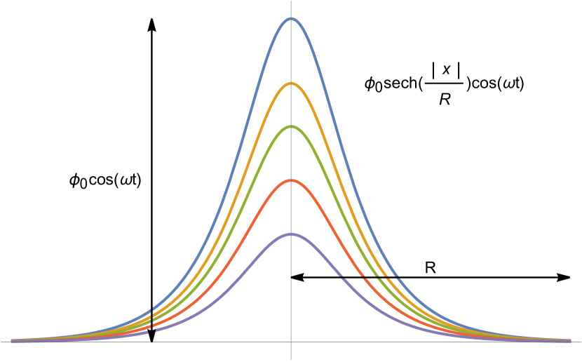
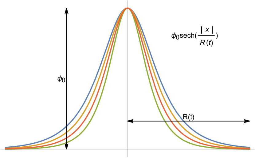
Figure 1: Plots of the spherically symmetric, oscillating field configuration $\phi\left({\bf x},t\right)$ (Left panel) and the oscillating field configuration $\phi\left({\bf x},t\right)$ with a time-dependent $R(t)$ for $\delta_{R}=1/5$ (Right panel). Different colors represent the distribution of the field at different moments.

To study the radiated EM field, we consider an analytic treatment in the limit of small coupling constant and expand the EM field as follows

$${\bf E}\left({\bf x},t\right) ={\bf E}_{0}\left({\bf x},t\right)+{\bf E}_{r}\left({\bf x},t\right)\,,$$ (30)

$${\bf B}\left({\bf x},t\right) ={\bf B}_{0}\left({\bf x},t\right)+{\bf B}_{r}\left({\bf x},t\right)\,.$$ (31)

${\bf E}_{r},{\bf B}_{r}$ represent the perturbed (radiated) EM field from the background ${\bf E}_{0},{\bf B}_{0}$, and ${\bf E}_{r},{\bf B}_{r}\ll{\bf E}_{0},{\bf B}_{0}$. The current $J_{s}^{\mu}$ in Eqs. (6) and (12) is proportional to the coupling constant, and we write the matter current as

$$\begin{split}J_{m}^{\mu}&=J_{0}^{\mu}+J_{p}^{\mu}\,.\end{split}$$ (32)

where $J_{0}^{\mu}$ sources the background EM field, and $J_{p}^{\mu}$ describes the plasma medium.

We note that, in the small coupling limit $g_{s\gamma}\phi_{0}\ll 1$ for the scalar, the coupling to the matter current in Eq. (8) leads to

$$\begin{split}\frac{1}{1+g_{s\gamma}\phi}J_{m}^{\mu}&\approx\left(1-g_{s\gamma}\phi\right)\left(J_{0}^{\mu}+J_{p}^{\mu}\right)\,.\end{split}$$ (33)

The above is a unique result in the scalar case, and the different coupling to the matter current may also allow us to distinguish the scalar and axion. However, to focus only on the different couplings to the EM field in this work, we ignore the other matter coupling $g_{s\gamma}\phi_{0}J^{\mu}_{m}$ even though it is the first order of perturbation.

The background electric and magnetic fields ${\bf E}_{0}$ and ${\bf B}_{0}$ are sourced by $J_{0}^{\mu}=(\rho_{0},{\bf J}_{0})$. For instance, the background matter fields can describe the magnetosphere of the neutron star or in the intergalactic medium. We note that $J_{0}^{\mu}$ is independent of the scalar or axion field configuration. We assume that the spatial extent of the scalar or axion configuration is much smaller than the coherent length of the background matter fields. Then, the background matter fields can be considered spatially constant. The perturbed electric and magnetic fields ${\bf E}_{r}$ and ${\bf B}_{r}$ correspond to radiated EM fields, which is sourced by $J_{s}^{\mu}$ which depends on the background EM fields ${\bf E}_{0}$, ${\bf B}_{0}$, and the scalar field $\phi$.

II.4 Plasma medium effect

Radiated EM fields can also be affected by the plasma medium $J^{\mu}_{p}$. To investigate the plasma medium effect on the EM radiation, we consider the EM wave propagation through the background plasma with the modified dispersion relation

$$k^{2}=\omega^{2}-\frac{\omega_{p}^{2}\omega}{\omega+i\nu}\,.$$ (34)

$\omega$ and $\nu$ are the EM radiation frequency and collision frequency, respectively. The plasma frequency $\omega_{p}$ is given by

$$\omega_{p}=\sqrt{\frac{4\pi n_{e}e^{2}}{m_{e}}}~{},$$ (35)

where $m_{e}$ is the electron mass, $e$ is the electron’s charge, and $n_{e}$ is the density of electrons.

In the collisionless limit, which is a good approximation to describe the hot plasma surrounding the compact stars and in the magnetosphere, $\omega\gg\nu$, the dispersion relation is given by

$$k^{2}=\omega^{2}-\omega_{p}^{2}\,.$$ (36)

Since we assume the background EM fields are spatially constant in this work, $\omega_{p}$ is assumed to be a constant, though $\omega_{p}$ depends on the spatially varying free electron density. In the following analysis, the plasma effect is involved in the perturbed equation in terms of the modified dispersion relation.

III Scalar case

From Eq. (21), the Maxwell equations for the background fields are given as

$$\begin{split}\nabla\times{\bf B}_{0}\left({\bf x},t\right)-\dot{\bf E}_{0}\left({\bf x},t\right)&={\bf J}_{0}\left({\bf x},t\right)\,,\\ \nabla\times{\bf E}_{0}\left({\bf x},t\right)+\dot{\bf B}_{0}\left({\bf x},t\right)&=0\,,\\ \nabla\times{\bf B}_{0}\left({\bf x},t\right)&=0\,,\\ \nabla\cdot{\bf E}_{0}\left({\bf x},t\right)&=\rho_{0}\left({\bf x},t\right)\,,\end{split}$$ (37)

and radiated EM fields obey the following equations

$$\begin{split}\nabla\times{\bf B}_{r}\left({\bf x},t\right)-\dot{\bf E}_{r}\left({\bf x},t\right)&={\bf J}_{p}\left({\bf x},t\right)+{\bf J}_{s}\left({\bf x},t\right)\,,\\ \nabla\times{\bf E}_{r}\left({\bf x},t\right)+\dot{\bf B}_{r}\left({\bf x},t\right)&=0\,,\\ \nabla\times{\bf B}_{r}\left({\bf x},t\right)&=0\,,\\ \nabla\cdot{\bf E}_{r}\left({\bf x},t\right)&=\rho_{p}\left({\bf x},t\right)+\rho_{s}\left({\bf x},t\right)\,.\end{split}$$ (38)

The plasma effect on the propagation of EM waves induced from the terms $\rho_{p}$ and ${\bf J}_{p}$ can be written as the dispersion relation. Thus, the EM radiation related to ${\bf E}_{r}$ and ${\bf B}_{r}$ is determined by the charge density and current of the scalar field $\rho_{s}$ and ${\bf J}_{s}$ coupled to the background EM fields:

$$\rho_{s}\left({\bf x},t\right) =-\frac{g_{s\gamma}}{1+g_{s\gamma}\phi\left({\bf x},t\right)}\nabla\phi\left({\bf x},t\right)\cdot{\bf E}_{0}\left({\bf x},t\right)\,,$$ (39)

$${\bf J}_{s}\left({\bf x},t\right) =\frac{g_{s\gamma}}{1+g_{s\gamma}\phi\left({\bf x},t\right)}\left[\dot{\phi}\left({\bf x},t\right){\bf E}_{0}\left({\bf x},t\right)-\nabla\phi\left({\bf x},t\right)\times{\bf B}_{0}\left({\bf x},t\right)\right]\,.$$ (40)

We denote the frequency of the oscillating scalar field, its mass, and the frequency of the oscillating radius of the scalar-field condensate by $\omega_{s}$, $m_{s}$, and $\omega_{so}$.

Specifying the three functions $\{{\bf E}_{0},{\bf B}_{0},\phi\}$, we can solve the differential equations for the EM radiation. Although those background fields are essentially determined by the background Maxwell equation with the background matter current $J^{\mu}_{0}$, we follow the previous studies Amin et al. (2021); Sen et al. (2022) and test several background configurations as the benchmark. In the following, we will consider three cases: constant and alternating background magnetic field with Eqs. (28); alternating magnetic field with Eq. (29). We apply these three settings to the scalar and axion fields in this section and the next section.

III.1 Constant magnetic field

First, we consider a simple setup with a constant magnetic field. We assume the background magnetic field is constant in $z$ direction, and the background electric field vanishes,

$$\begin{split}{\bf E}_{0}\left({\bf x},t\right)&=0\,,\\ {\bf B}_{0}\left({\bf x},t\right)&=B_{0}\hat{\bf z}\,,\end{split}$$ (41)

where $\hat{\bf z}$ is the unit vector in the z direction. Substituting Eqs. (41) and (28) into Eqs. (39) and (40), we obtain the charge density and current,

$$\begin{split}\rho_{s}\left({\bf x},t\right)&=0\,,\end{split}$$ (42)

$$\begin{split}{\bf J}_{s}\left({\bf x},t\right)&=\frac{g_{s\gamma}}{1+g_{s\gamma}\phi\left(\mathbf{x},t\right)}\left[-\nabla\phi\left(\mathbf{x},t\right)\times\mathbf{B}_{0}\left(\mathbf{x},t\right)\right]\\ &\approx\frac{g_{s\gamma}\phi_{0}B_{0}}{R}\cos\left(m_{s}t\right)\mathrm{sech}\left(\frac{\left|\mathbf{x}\right|}{R}\right)\tanh\left(\frac{\left|\mathbf{x}\right|}{R}\right)\hat{\mathbf{x}}\times\hat{\mathbf{z}}\,.\end{split}$$ (43)

Here, we used $g_{s\gamma}\phi_{0}\ll 1$ in the second line of Eq. (43), and $\hat{\bf x}$ is the unit vector in the radial direction. Using the above source, we solve the Maxwell equations and derive the radiated EM field ${\bf E}_{r}\left({\bf x},t\right)$ and ${\bf B}_{r}\left({\bf x},t\right)$.

In general, the Maxwell equation for the EM field $A^{\mu}\left({\bf x},t\right)$ with a source $J^{\mu}\left({\bf x},t\right)$ is written as

$$\Box A^{\mu}\left({\bf x},t\right)=-J^{\mu}\left({\bf x},t\right)\,,$$ (44)

where $A^{\mu}=\left(A^{0},{\bf A}\right)$ and $J^{\mu}=\left(\rho,{\bf J}\right)$. We can solve the above equation by the Green’s function method, and the corresponding retarded Green’s function is written as follows:

$$\begin{split}G\left({\bf x},t;{\bf x}^{\prime},t^{\prime}\right)&=-\frac{1}{2\pi}\int\frac{d\omega}{4\pi\left|{\bf x}-{\bf x}^{\prime}\right|}e^{-i\omega(t-t^{\prime})+ik_{s}\left|{\bf x}-{\bf x}^{\prime}\right|}\theta(k_{s}^{2})\\ &\qquad-\frac{1}{2\pi}\int\frac{d\omega}{4\pi\left|{\bf x}-{\bf x}^{\prime}\right|}e^{-i\omega(t-t^{\prime})-\sqrt{|k_{s}^{2}|}\left|{\bf x}-{\bf x}^{\prime}\right|}\theta(-k_{s}^{2})\,,\end{split}$$ (45)

$k_{s}$ includes the plasma effect, $k_{s}=\sqrt{m_{s}^{2}-\omega_{p}^{2}}$, and $\theta(k_{s}^{2})$ is the Heaviside step function. If the frequency of EM radiation is smaller than that of the plasma ($\omega\sim m_{s}<\omega_{p}$), the radiation is exponentially damped. Furthermore, we assume the plasma frequency is smaller than the scalar field mass.

The vector potential ${\bf A}\left({\bf x},t\right)$ is expressed in terms of the Green’s function as

$$\begin{split}{\bf A}\left({\bf x},t\right)&=\int d^{3}\mathbb{x^{\prime}}dt^{\prime}G\left({\bf x},t;{\bf x}^{\prime},t^{\prime}\right){\bf J}_{s}\left(\mathbb{x^{\prime}},t^{\prime}\right)\\ &=\frac{g_{s\gamma}\phi_{0}B_{0}}{4\pi R}\left[\int_{0}^{\infty}|x^{\prime}|^{2}dx^{\prime}\int_{0}^{\pi}\sin\theta^{\prime}d\theta^{\prime}\int_{0}^{2\pi}d\varphi^{\prime}\frac{1}{\left|{\bf x}-\mathbb{x^{\prime}}\right|}\right.\\ &\qquad\qquad\qquad\left.\cos\left(m_{s}t-k_{s}\left|{\bf x}-\mathbb{x^{\prime}}\right|\right){\rm sech}\left(\frac{x^{\prime}}{R}\right)\tanh\left(\frac{x^{\prime}}{R}\right)\right]\hat{\bf x}\times\hat{\bf z}\\ &\approx\frac{g_{s\gamma}\phi_{0}B_{0}}{2xR}\left\{\int_{0}^{\infty}|x^{\prime}|^{2}dx^{\prime}\int_{-1}^{1}d(\cos\theta^{\prime})\right.\\ &\qquad\qquad\qquad\left.\cos\left[m_{s}t-k_{s}\left(x-x^{\prime}\cos\theta^{\prime}\right)\right]{\rm sech}\left(\frac{x^{\prime}}{R}\right)\tanh\left(\frac{x^{\prime}}{R}\right)\right\}\hat{\bf x}\times\hat{\bf z}\,.\end{split}$$ (46)

$\theta^{\prime}$ is the angle between ${\bf x}$ and ${\bf x}^{\prime}$, and we used an approximation

$$|{\bf x}-{\bf x}^{\prime}|\approx x-\frac{{\bf x}\cdot{\bf x}^{\prime}}{x}=x-x^{\prime}\cos\theta^{\prime}$$ (47)

in the third equality of Eq. (46). The radiated electric and magnetic fields are written by the corresponding EM field $A^{\mu}$ as

$$\begin{split}{\bf E}_{r}\left({\bf x},t\right)&=-\nabla A_{0}\left({\bf x},t\right)-\partial_{t}\mathbb{A}\left({\bf x},t\right)\,,\\ {\bf B}_{r}\left({\bf x},t\right)&=\nabla\times\mathbb{A}\left({\bf x},t\right)\,,\end{split}$$ (48)

and the Poynting flux for the radiated electric and magnetic field is defined by

$${\bf S}\left({\bf x},t\right)={\bf E}_{r}\left({\bf x},t\right)\times{\bf B}_{r}\left({\bf x},t\right)\,.$$ (49)

Since the radiated power per unit solid angle is expressed as

$$\frac{dP}{d\Omega}=|{\bf x}|^{2}{\bf S}\cdot\hat{\bf x}~{},$$ (50)

we obtain the time-averaged radiation power as

$$\mathcal{P}=|{\bf x}|^{2}\int\bar{\bf S}\cdot\hat{\bf x}d\Omega=4\pi|{\bf x}|^{2}|\bar{\bf S}|\,,$$ (51)

where $\bar{\bf S}=\frac{1}{T}\int_{0}^{T}{\bf S}dt$ and $T=\frac{2\pi}{m_{s}}$. In the calculation of the basis vectors, we used the following result:

$$\begin{split}&\hat{\bf x}\cdot\left\{(\hat{\bf x}\times\hat{\bf z})\times\left[\hat{\bf x}\times(\hat{\bf x}\times\hat{\bf z})\right]\right\}\\ &=\hat{\bf x}\cdot\{\hat{\bf x}(\hat{\bf x}\times\hat{\bf z})\cdot(\hat{\bf x}\times\hat{\bf z})-(\hat{\bf x}\times\hat{\bf z})[(\hat{\bf x}\times\hat{\bf z})\cdot\hat{\bf x}]\}\\ &=\hat{\bf x}\cdot(\hat{\bf x}|\hat{\bm{\varphi}}||\hat{\bm{\varphi}}|)\\ &=|\hat{\bf x}|^{2}|\hat{\bm{\varphi}}|^{2}\\ &=1\,.\end{split}$$ (52)

Here, we denote the unit vector in the azimuth direction by $\hat{\bm{\varphi}}$. $\nabla A_{0}$ does not contribute to the radiated power because of the absence of the charge density $\rho_{s}\left({\bf x},t\right)=0$. The charge density vanishes because the background electric field is assumed to be zero. In the next two subsections, this result will apply to the other two cases for alternating magnetic fields.

According to the above definitions and relations, the EM radiation emitted from the scalar field in the presence of a constant external magnetic field is obtained as

$$\mathcal{P} =\frac{1}{128k_{s}}\pi g_{s\gamma}^{2}\phi_{0}^{2}B_{0}^{2}R^{2}m_{s}\left[4iQ^{0}_{-}(k_{s}R)+k_{s}RQ^{1}_{+}(k_{s}R)\right]^{2}$$

$$=\frac{\pi g_{s\gamma}^{2}\phi_{0}^{2}B_{0}^{2}}{128m_{s}^{2}\sqrt{1-\xi_{s}^{2}}}\ R_{s*}^{2}\left[4iQ^{0}_{-}(\sqrt{1-\xi_{s}^{2}}R_{s*})+\sqrt{1-\xi_{s}^{2}}R_{s*}Q^{1}_{+}(\sqrt{1-\xi_{s}^{2}}R_{s*})\right]^{2},$$ (53)

where $R_{s*}$ is the dimensionless size variable $R_{s*}:=m_{s}R$, and $\xi_{s}$ is newly introduced parameter as $\xi_{s}:=\omega_{p}/m_{s}$, and

$$Q^{n}_{\pm}(x):=\psi^{(n)}\left(\frac{1}{4}-i\frac{x}{4}\right)-\psi^{(n)}\left(\frac{3}{4}-i\frac{x}{4}\right)\pm\psi^{(n)}\left(\frac{1}{4}+i\frac{x}{4}\right)\mp\psi^{(n)}\left(\frac{3}{4}+i\frac{x}{4}\right)$$ (54)

with the Polygamma function by $\psi^{n}(x)$, which arises from the integral in Eq. (46). Note that for real variable $x$, $Q^{0}_{\pm}(x)$ and $Q^{1}_{\pm}(x)$ are purely imaginary and real functions, respectively, therefore $\mathcal{P}$ is a real function of $R_{*}$, we will discuss the behavior of radiated power in Sec V.

It is clear from Eq. (53) that the radiated power depends on the size of $R_{s*}$. When $\omega_{p}$ is negligible, the peak in radiation occurs for $R_{s*}\sim 0.84$, and when $R_{s*}\gg 0.84$, radiation is suppressed. For $\omega_{p}$ is non-negligible, the radiation peak for $R_{s*}\sim\frac{0.84}{\sqrt{1-\xi_{s}^{2}}}$. Thus, the resonant effect occurs when plasma frequency is close to the scalar mass scale ($\xi_{s}^{2}\sim 1$), and the resonant effect can enhance the radiated power when the size of the scalar field $R$ is much larger than the inverse scalar mass scale $m^{-1}$.

However, the resonant effect does not always enhance the radiated power. For $R_{s*}\ll 1/\sqrt{1-\xi_{s}^{2}}$, $\mathcal{P}$ becomes

$$\mathcal{P}\approx\frac{\pi g_{s\gamma}^{2}\phi_{0}^{2}B_{0}^{2}}{32m_{s}^{2}}\sqrt{1-\xi_{s}^{2}}R_{s*}^{4}\left[\psi^{(1)}(1/4)-\psi^{(1)}(3/4)\right]^{2}\,.$$ (55)

It shows that radiation generated under the condition of $\omega_{p}=0$ is stronger than that generated under the resonance condition ($m_{s}\sim\omega_{p}$). In the following, we will explore a similar resonant effect that can occur in an alternating magnetic field background.

III.2 Alternating magnetic field

Next, we consider the alternating magnetic field as the background, which may appear around the spinning neutron stars Pons and Geppert (2007); Gourgouliatos and Cumming (2014). The background electric and magnetic fields are assumed to be

$$\begin{split}{\bf E}_{0}\left({\bf x},t\right)&=0\,,\\ {\bf B}_{0}\left({\bf x},t\right)&=B_{0}\cos\left(\Omega t\right)\hat{\bf z}\,,\end{split}$$ (56)

where $\Omega$ is the frequency of the magnetic field, and we ignore the initial phase shift of the frequency. Substituting Eqs. (56) and (28) into Eqs. (39) and (40), the charge density and current can be expressed as

$$\begin{split}\rho_{s}\left({\bf x},t\right)&=0\,.\end{split}$$ (57)

$$\begin{split}{\bf J}_{s}\left({\bf x},t\right)&\approx\frac{g_{s\gamma}\phi_{0}B_{0}}{R}\cos\left(m_{s}t\right){\rm sech}\left(\frac{\left|{\bf x}\right|}{R}\right)\tanh\left(\frac{\left|{\bf x}\right|}{R}\right)\cos\left(\Omega t\right)\hat{\bf x}\times\hat{\bf z}\,,\end{split}$$ (58)

As in the previous subsection, we compute the time-averaged radiated power and obtain the following expression in both $\omega_{s}>\Omega$ and $\Omega>\omega_{s}$ cases,

$$\begin{split}\mathcal{P}&=\dfrac{\pi g_{s\gamma}^{2}\phi_{0}^{2}B_{0}^{2}}{256m_{s}^{2}}R_{s*}^{2}\left\{\dfrac{1+\zeta_{s}}{f_{s+}}\left[4iQ^{0}_{-}(f_{s+}R_{s*})+f_{s+}R_{s*}Q^{1}_{+}(f_{s+}R_{s*})\right]^{2}\theta(f_{s+}^{2})\right.\\ &\qquad\left.+\dfrac{1-\zeta_{s}}{f_{s-}}\left[4iQ^{0}_{-}(f_{s-}R_{s*})+f_{s-}R_{s*}Q^{1}_{+}(f_{s-}R_{s*})\right]^{2}\theta(f_{s-}^{2})\right\}\,,\end{split}$$ (59)

where $f_{s\pm}=\sqrt{(1\pm\zeta_{s})^{2}-\xi_{s}^{2}}$, $\zeta_{s}$ is a parameter: $\zeta_{s}=\Omega/m_{s}$ and the radiation be suppressed when $f_{\pm}^{2}<0$. As Eq. (59) shows, it same as Eq. (53), when $\Omega=0$. The radiation peaks for $R_{s*}\sim\frac{0.84}{\sqrt{(1\pm\zeta_{s})^{2}-\xi_{s}^{2}}}$, thus, the resonance effect depends on both the $\omega_{p}$ and $\Omega$.

For $R_{s*}\ll 1/\sqrt{(1\pm\zeta_{s})^{2}-\xi_{s}^{2}}$, Eq. (59) becomes

$$\mathcal{P}\approx\frac{\pi g_{s\gamma}^{2}\phi_{0}^{2}B_{0}^{2}}{64m_{s}^{2}}R_{s*}^{4}\left((1+\zeta_{s})f_{s+}\theta(f_{s+}^{2})+(1-\zeta_{s})f_{s-}\theta(f_{s-}^{2})\right)\left[\psi^{(1)}(1/4)-\psi^{(1)}(3/4)\right]^{2}\,,$$ (60)

The above expression clearly shows that the resonance effect appears when $\omega_{p}=0$ and $m_{s}\sim\Omega$. The scalar-field oscillation can emit EM radiation more efficiently than other resonance effects that occur when $m_{s}\sim\omega_{p}$ and $\Omega=0$.

III.3 Radial oscillation of scalar condensate

Finally, we consider the case in which the radius of the scalar field oscillates. As in Eq. (56), we consider the alternating background magnetic field and assume the background electric field vanishes. Moreover, we ignore the plasma effect for simplicity. Substituting Eqs. (56) and (29) into Eqs. (39) and (40), the charge density and current are expressed as

$$\begin{split}\rho_{s}\left({\bf x},t\right)&=0\,,\end{split}$$ (61)

$$\begin{split}{\bf J}_{s}\left({\bf x},t\right)&\approx\frac{g_{s\gamma}\phi_{0}B_{0}\cos\left[\Omega t\right]}{R\left(1+\delta_{R}\cos[\omega_{so}t]\right)}{\rm sech}\left[\frac{\left|{\bf x}\right|}{R\left(1+\delta_{R}\cos[\omega_{so}t]\right)}\right]\\ &\qquad\times\tanh\left[\frac{\left|{\bf x}\right|}{R\left(1+\delta_{R}\cos[\omega_{so}t]\right)}\right]\hat{\bf x}\times\hat{\bf z}\,.\end{split}$$ (62)

We note that in Eq. (62), $\delta_{R}=0$ leads to the current density in the case of the constant magnetic field, where the frequency of the alternating magnetic field mimics the role of the frequency of the oscillating scalar field in Eq. (43). Consequently, the generated EM radiation has the same characteristics as the case constant magnetic field, in which $\omega_{p}$ is negligible. We cannot obtain the analytic form of the time-averaged radiated power for $\delta_{R}\ll 1$, and we will discuss the numerical results in Sec V.

IV Axion case

In this section, we apply the background setting in the scalar to the axion field and analyze the radiation power. From Eq. (25), the Maxwell equations for the background field are given as

$$\begin{split}\nabla\times{\bf B}_{0}\left({\bf x},t\right)-\dot{\bf E}_{0}\left({\bf x},t\right)&={\bf J}_{0}\left({\bf x},t\right)\,,\\ \nabla\times{\bf E}_{0}\left({\bf x},t\right)+\dot{\bf B}_{0}\left({\bf x},t\right)&=0\,,\\ \nabla\times{\bf B}_{0}\left({\bf x},t\right)&=0\,,\\ \nabla\cdot{\bf E}_{0}\left({\bf x},t\right)&=\rho_{0}\left({\bf x},t\right)\,,\end{split}$$ (63)

and radiated EM fields are given as

$$\begin{split}\nabla\times{\bf B}_{r}\left({\bf x},t\right)-\dot{\bf E}_{r}\left({\bf x},t\right)&={\bf J}_{p}\left({\bf x},t\right)+{\bf J}_{s}\left({\bf x},t\right)\,,\\ \nabla\times{\bf E}_{r}\left({\bf x},t\right)+\dot{\bf B}_{r}\left({\bf x},t\right)&=0\,,\\ \nabla\times{\bf B}_{r}\left({\bf x},t\right)&=0\,,\\ \nabla\cdot{\bf E}_{r}\left({\bf x},t\right)&=\rho_{p}\left({\bf x},t\right)+\rho_{s}\left({\bf x},t\right)\,.\end{split}$$ (64)

As in the case of the scalar field, we drop the terms $\rho_{p}$ and ${\bf J}_{p}$ in the above equations and evaluate the plasma effect as the modified dispersion relation. The EM radiation depends on the charge density and current of the axion field coupled to the background EM fields,

$$\rho_{s}\left({\bf x},t\right) =-g_{a\gamma}\nabla\phi\left({\bf x},t\right)\cdot{\bf B}_{0}\left({\bf x},t\right)\,,$$ (65)

$${\bf J}_{s}\left({\bf x},t\right) =g_{a\gamma}\left[\dot{\phi}\left({\bf x},t\right){\bf B}_{0}\left({\bf x},t\right)+\nabla\phi\left({\bf x},t\right)\times{\bf E}_{0}\left({\bf x},t\right)\right]\,.$$ (66)

To demonstrate the qualitative comparison with the scalar field case, we consider the EM radiation generated by the axion field based on the same three settings assumed in the previous section. We denote the frequency of the oscillating axion field, its mass, and the frequency of the oscillating radius of the axion-field condensate by $\omega_{a}$, $m_{a}$, and $\omega_{ao}$ for the axion field.

IV.1 Constant magnetic field

First, we apply the settings in section III.1 to the axion field. Substituting Eqs. (41) and (28) into Eqs. (65) and (66), we obtain

$$\begin{split}\rho_{s}\left({\bf x},t\right)&=-g_{a\gamma}\nabla\phi\left({\bf x},t\right)\cdot{\bf B}_{0}\left({\bf x},t\right)\\ &\approx\frac{g_{a\gamma}\phi_{0}B_{0}}{R}\cos(m_{a}t)\mathrm{sech}\left(\frac{\left|{\bf x}\right|}{R}\right)\tanh\left(\frac{\left|{\bf x}\right|}{R}\right)\mathbb{\hat{x}}\cdot\hat{\bf z}\,,\end{split}$$ (67)

$$\begin{split}{\bf J}_{s}\left({\bf x},t\right)&=g_{a\gamma}\dot{\phi}\left({\bf x},t\right){\bf B}_{0}\left({\bf x},t\right)\\ &\approx-g_{a\gamma}m_{a}\phi_{0}B_{0}\sin\left(m_{a}t\right)\mathrm{sech}\left(\frac{\left|{\bf x}\right|}{R}\right)\hat{\bf z}\,,\end{split}$$ (68)

It is worth mentioning that the charge density does not vanish in the axion case despite the same background field configurations. Applying the Green’s function method, we obtain the radiated EM field $A^{\mu}$. However, the time-averaged radiation power in the case of axion is different from that of the scalar due to the different coupling to the EM field,

$$\mathcal{P}=|{\bf x}|^{2}\int\bar{\bf S}\cdot\hat{\bf x}d\Omega=\frac{8}{3}\pi|{\bf x}|^{2}|\bar{\bf S}|\,.$$ (69)

where $\bar{\bf S}=\frac{1}{T}\int_{0}^{T}{\bf S}dt$ and $T=\frac{2\pi}{m_{a}}$. Compared with the scalar field case, the different coupling to the EM field results in the different basis vectors in the current ${\bf J}_{s}$. In the calculation of the basis vectors, we used the following result:

$$\hat{\bf x}\cdot[\hat{\bf z}\times(\mathbb{\hat{x}}\times\hat{\bf z})]$$

$$= \hat{\bf x}\cdot[\hat{\bf x}|\hat{\bf z}|^{2}-\hat{\bf z}(|\hat{\bf x}||\hat{\bf z}|\cos\theta)]$$

$$= |\hat{\bf x}|^{2}|\hat{\bf z}|^{2}-|\hat{\bf x}|^{2}|\hat{\bf z}|^{2}\cos\theta^{2}$$

$$= \sin^{2}\theta~{}.$$ (70)

We note that $\nabla\mathbb{A}_{0}$ does not contribute to the radiated power, as in the scalar field case, but for a different reason. The charge density does not vanish because the background magnetic field is nonzero. In calculating $dP/d\Omega$, $(\mathbb{E}_{r}\times\mathbb{B}_{r})\cdot\hat{\bf x}$ includes $\nabla\mathbb{A}_{0}$, however, it is proportional to $\left[\hat{\bf x}\times\left(\hat{\bf x}\times\hat{\bf z}\right)\right]\cdot\hat{\bf x}=0$. This result will again apply to the other two cases for alternating magnetic fields in the next two subsections.

Based on the above consideration, the time-averaged radiated power in the presence of a constant external magnetic field and plasma is given by

$$\mathcal{P}=\frac{4\pi^{5}g_{a\gamma}^{2}\phi_{0}^{2}B_{0}^{2}}{3m_{a}^{2}\sqrt{1-\xi_{a}^{2}}}R_{a*}^{4}\mathrm{csch}\left(\pi\sqrt{1-\xi_{a}^{2}}R_{a*}\right)^{4}\sinh\left(\frac{\pi\sqrt{1-\xi_{a}^{2}}R_{a*}}{2}\right)^{6}~{},$$ (71)

where $\xi_{a}=\omega_{p}/m_{a}$, $R_{a*}=m_{a}R$. The above results are consistent with results in the existing works Amin et al. (2021); Sen et al. (2022). The radiated power peaks for $R_{a*}\sim\frac{1.38}{\sqrt{1-\xi_{a}^{2}}}$ and when $R_{a*}\gg\frac{1.38}{\sqrt{1-\xi_{a}^{2}}}$, the radiated power is exponentially suppressed.

IV.2 Alternating magnetic field

Next, we apply the settings in section III.2 to the axion field. Substituting Eqs. (56) and (28) into Eqs. (65) and (66), we obtain the charge density and current,

$$\begin{split}\rho_{s}\left({\bf x},t\right)&\approx\frac{g_{a\gamma}\phi_{0}}{R}\cos\left(m_{a}t\right)\mathrm{sech}\left(\frac{\left|{\bf x}\right|}{R}\right)\tanh\left(\frac{\left|{\bf x}\right|}{R}\right)B_{0}\cos\left(\Omega t\right)\hat{\bf x}\cdot\hat{\bf z}\,.\end{split}$$ (72)

$$\begin{split}{\bf J}_{s}\left({\bf x},t\right)&\approx-g_{a\gamma}m_{a}\phi_{0}\sin\left(m_{a}t\right)\mathrm{sech}\left[\frac{\left|{\bf x}\right|}{R}\right]B_{0}\cos\left(\Omega t\right)\hat{\bf z}\,,\end{split}$$ (73)

The corresponding time-averaged radiated power is given by

$$\begin{split}\mathcal{P}&=\frac{2\pi^{5}g_{a\gamma}^{2}\phi_{0}^{2}B_{0}^{2}}{3m_{a}^{2}}R_{a*}^{4}\left[\frac{1+\zeta}{f_{a+}}{\rm csch}\left(\pi f_{a+}R_{a*}\right)^{4}\sinh\left(\frac{\pi f_{a+}R_{a*}}{2}\right)^{6}\theta(f_{a+}^{2})\right.\\ &\qquad\left.+\frac{1-\zeta}{f_{a-}}{\rm csch}\left(\pi f_{a-}R_{a*}\right)^{4}\sinh\left(\frac{\pi f_{a-}R}{2}\right)^{6}\theta(f_{a-}^{2})\right]\,,\end{split}$$ (74)

where $f_{a\pm}=\sqrt{(1\pm\zeta_{a})^{2}-\xi_{a}^{2}}$, $\zeta_{a}=\Omega/m_{a}$ and the radiation be exponentially suppressed when $f_{a\pm}$ is not real. According to Eq. (74), the peak in radiation occurs for two different values of the field radius: $R_{a*}\sim\frac{1.38}{\sqrt{(1-\zeta_{a})^{2}-\xi_{a}^{2}}}$ and $R_{a*}\sim\frac{1.38}{\sqrt{(1+\zeta_{a})^{2}-\xi_{a}^{2}}}$.

IV.3 Radial oscillation of axion condensate

Finally, we apply the settings in section III.3 to the axion field. Substituting Eqs. (56) and (29) into Eqs. (65) and (66), the charge density and current are

$$\begin{split}\rho_{s}\left({\bf x},t\right)&\approx\frac{g_{a\gamma}\phi_{0}}{R\left(1+\delta_{R}\cos[\omega_{ao}t]\right)}\\ &\qquad\times\mathrm{sech}\left[\frac{\left|{\bf x}\right|}{R\left(1+\delta_{R}\cos[\omega_{ao}t]\right)}\right]\tanh\left[\frac{\left|{\bf x}\right|}{R\left(1+\delta_{R}\cos[\omega_{ao}t]\right)}\right]B_{0}\hat{\bf x}\cdot\hat{\bf z}\,.\end{split}$$ (75)

$$\begin{split}{\bf J}_{s}\left({\bf x},t\right)&\approx-\frac{\delta_{R}~{}\omega_{ao}\left|{\bf x}\right|g_{s\gamma}\phi_{0}\sin\left[\omega_{ao}t\right]\cos\left[\Omega t\right]}{R\left(1+\delta_{R}\cos[\omega_{ao}t]\right)^{2}}\\ &\qquad\times{\rm sech}\left[\frac{\left|{\bf x}\right|}{R\left(1+\delta_{R}\cos[\omega_{ao}t]\right)}\right]\tanh\left[\frac{\left|{\bf x}\right|}{R\left(1+\delta_{R}\cos[\omega_{ao}t]\right)}\right]B_{0}\hat{\bf z}\,,\end{split}$$ (76)

We note that the current vanishes when $\delta_{R}=0$, ${\bf J}_{s}\left({\bf x},t\right)\approx 0$. Thus, we require $\delta_{R}\neq 0$ for the axion field to radiate in the above background field setups. We will discuss the numerical results for nonzero $\delta_{R}$ in Sec V.

V Comparison: scalar vs. axion

V.1 Qualitative behaviors of radiation power

Based on the analysis in the previous two sections, we show and compare numerical results of the EM radiation power for three different cases with the scalar and axion fields. We plot the radiated power in the constant magnetic field in Fig. 2, where the plasma frequency is smaller than the mass scale.

As we mentioned in the sections III.1 and IV.1, peaks in the radiation power for the scalar and axion are characterized by $R_{*}\sim C_{i}/\sqrt{1-\xi^{2}}$, where $R_{*}$ denotes the product of the mass of axion/scalar with $R$, and $C_{i}$ is a constant, we denote it by $C_{a}$ and $C_{s}$ for the axion and scalar, respectively.

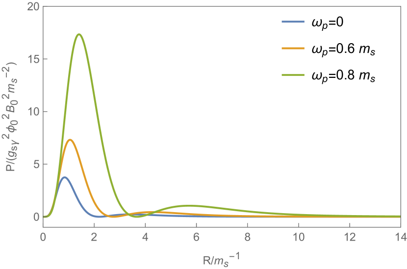
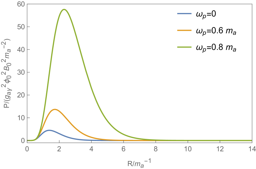
Figure 2: The radiated power as a function of $R$ in the case of the constant magnetic field for the scalar (Left panel) and axion (Right panel).

Fig. 2 shows that values of $R$ at the radiation peak for scalar and axion are not entirely identical ($0.84\sim C_{s}<C_{a}\sim 1.38$). For both scalar and axion, the radiation power is suppressed when $R_{*}\gg C_{i}/\sqrt{1-\xi^{2}}$. The physical origin of this suppression is destructive interference between the emitted EM waves, which are emitted in phases from different locations within the particles. It is remarkable that for the scalar, one bump ($C_{s}\sim 3.43$) occurs in the radiated power in addition to the radiation peak, which cannot be observed for the axion. This extra bump will become significant in light of the resonance effect shown in the left panel of Fig. 3.

We plot the radiated power in the alternating magnetic field in Figs. 3 and 4.

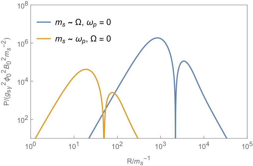
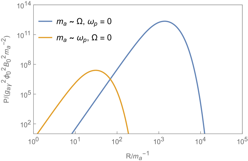
Figure 3: The radiated power as a function of $R$ in the case of the alternating magnetic field for the scalar (Left panel) and axion (Right panel).

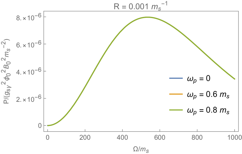
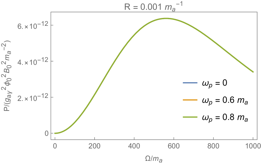
Figure 4: The radiated power as a function of $\Omega$ in the case of the alternating magnetic field with $R=0.001\omega^{-1}$ for the scalar (Left panel) and axion (Right panel).

In Fig. 3, we consider two types of resonance effects; $\omega\sim\Omega=0.999m$ and $\omega_{p}=0$; $\omega\sim\omega_{p}=0.999m$ and $\Omega=0$. The radiation peaks for scalar and axion are denoted by $R_{*}\sim\frac{C_{i}}{\sqrt{(1-\zeta)^{2}-\xi^{2}}}$ and $R_{*}\sim\frac{C_{i}}{\sqrt{(1+\zeta)^{2}-\xi^{2}}}$. It is clear that the resonance of the oscillating scalar/axion field with the alternating magnetic field causes more efficient radiation than the resonance of an oscillating field with a background plasma. The difference between scalar and axion is significant due to the resonance effect, which provides more possibilities for distinguishing them. In Fig. 4, we can understand how the radiated power varies with the magnetic field frequency at different plasma frequencies. When $R=0.001m^{-1}$, the resonance condition is approximately given as $\Omega\sim C_{i}/R\gg m,\omega_{p}$, so the plasma effect on the radiated power is negligible. Consequently, the plots for different plasma frequencies overlap each other.

We finally plot the radiated power in the radial oscillation of the scalar/axion field in Fig. 5. we have chosen $\delta_{R}=1/1000$ as a benchmark value. To make an intuitive comparison between the radiation power behavior of scalar and axion, the radiation power values for $\Omega=0.6\omega_{ao}$ and $\Omega=\omega_{ao}$ are multiplied by $10^{1}$ and $10^{4}$ respectively in the case of axion.

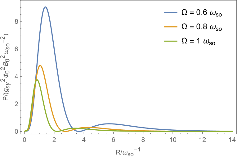
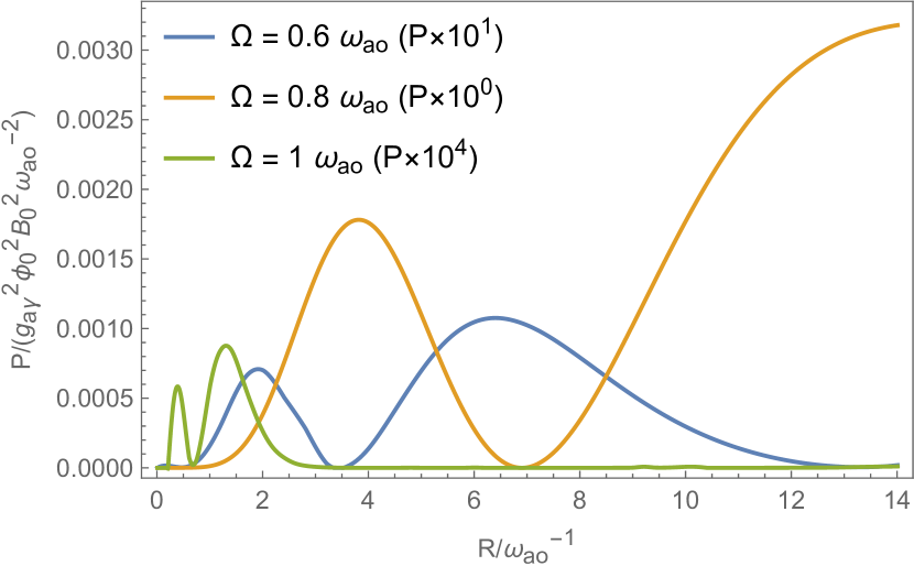
Figure 5: The radiated power as a function of $R$ in the case of radial oscillation with $\delta_{R}=1/1000$ for the scalar (Left panel) and axion (Right panel).

In the scalar case, the radiated power has the same characteristic as the constant magnetic fields, where we can ignore the plasma effect, and there are no additional resonance effects. In the case of the axion, unlike the scalar, the resonance enhancement effect occurs, and there are two bumps in the radiated power.

V.2 Detectability

It is of great significance that we analyze the detectability of the EM signals generated by scalar and axion and the possibility to distinguish them by observation. We consider the mass range of $10^{-7}$ eV - $10^{-2}$ eV, where the corresponding frequency is $24$ MHz - $2400$ GHz, and existing and forthcoming radio telescopes can detect this frequency range. Denoting distance between the source and the Earth by $d$, we obtain the flux of EM radiation reaching Earth as $F=L/(4\pi d^{2})$ for the luminosity $L=\mathcal{P}$. The spectral flux density can be calculated as $S=F/\triangle B$, where $\triangle B\approx\omega/2\pi$ is the signal bandwidth and $\omega$ is the frequency of the EM signal. Then, the spectral flux density can be written as

$$S=\frac{L}{4\pi d^{2}\triangle B}=\frac{\mathcal{P}}{2\omega d^{2}}\,.$$ (77)

In particular, for the case of alternating magnetic field, although the radiated power has contributions of two different frequencies $|m-\Omega|$ and $m+\Omega$, we consider that the detected spectral line has a frequency of $m/2\pi$ when $m\sim\Omega$.

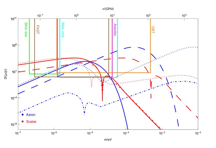
Figure 6: The blue and red curves represent the spectral flux densities of axion and scalar, respectively. We plot spectral flux density in the four cases: the constant magnetic field which $\omega_{p}=0$ (solid curves); the alternating magnetic field with $m\sim\omega_{p}=0.999m$ and $\Omega=0$ (dashed curves), and with $m\sim\Omega=0.999m$ and $\omega_{p}=0$ (dotted curves); the radial oscillating with $\omega_{o}\sim\Omega=0.999m$ (dot-dashed curves). The sensitivity curves of the SKA-low, SKA-mid, FAST, Arecibo, and GBT are shown for $t_{{\rm obs}}=1{\rm hr}$.

In Fig. 6, we plot four cases of spectral flux densities for different particle masses: The constant magnetic field which $\omega_{p}=0$; alternating magnetic field with $m\sim\omega_{p}$ and $m\sim\Omega$; radial oscillation with $\omega_{o}\sim\Omega$. We also plot detection sensitivities for various telescopes: The sensitivities curves contain Square Kilometre Array (SKA) has the frequency form 50 MHz - 350 MHZ (SKA-low) and 350 MHz to 14 GHz (SKA-mid) Dewdney et al. (2009); Five hundred meter Aperture Spherical Telescope (FAST) has the frequency 70 MHz to 8 GHz Nan et al. (2011); Arecibo Observatory (Arecibo) covered frequencies from 300 MHz-10 GHz Giovanelli et al. (2005); the existing Green Bank Telescope (GBT) has a 100 by 110 meter active surface and can cover the frequency range of 290 MHz - 115.3 GHz Prestage et al. (2009); White et al. (2022).

Following Ref. Bai and Hamada (2018), we assume $B_{0}=10^{10}{\rm G}$ and $d=1{\rm kpc}$ as benchmark parameters. For the axion case, the relation between the characteristic size of axion star $R$ and mass $m_{a}$ is given as

$$R=0.02{\rm m}\times\left(\frac{4\times 10^{12}{\rm GeV}}{f_{a}}\right)^{1/2}\left(\frac{10^{-5}{\rm eV}}{m_{a}}\right)^{1/2}\left(\frac{M_{a}}{10^{-16}M_{\odot}}\right)^{0.3}\,,$$ (78)

where $f_{a}$ and $M_{a}$ are decay constant and axion star mass respectively. Considering the QCD axion, we fix the $m_{a}f_{a}=(2\times 10^{8}{\rm eV})^{2}$ Bai and Hamada (2018). The coupling constant can be rewritten as $g_{a\gamma}=\alpha c_{\gamma}/(\pi f_{a})$, where $\alpha$ is the fine structure constant, $c_{\gamma}$ is a model-dependent number, and its value can vary from $\sim{\cal O}(1)$ to many orders of magnitude higher Choi and Im (2016); Kaplan and Rattazzi (2016); Agrawal et al. (2018); Kouvaris et al. (2024). For a dense axion star, $\phi_{0}\sim{\cal O}(1)f_{a}$ Kyriazis (2022), and we fix the model parameters as $g_{a\gamma}\phi_{0}=10^{-2}$.

For the comparison of EM signal emission from the scalar with that from the axion, we choose the same parameters for the scalar as those for the axion, which allows us to focus on the different coupling to photons and their characteristic observational signatures. Although we can consider a simple fundamental scalar field where the mass and coupling constant are free parameters, the modified gravity theory can be embedded into our consideration. If the scalar field originates from the scalar-tensor theory of gravity, the mass and coupling constant can be arbitrary Brans and Dicke (1961); Horndeski (1974); Fujii and Maeda (2003); Faraoni and Faraoni (2004). Moreover, even if we consider the DE model of scalar-tensor theory, the mass range can be much larger than the DE scale due to the chameleon mechanism Khoury and Weltman (2004a, b). The chameleon mechanism is one of the screening mechanisms to hide the scalar-mediated long-range fifth force in the local tests of gravity. Naturally, we expect that the viable DE models of the scalar-tensor theory have the chameleon mechanism, and it is plausible to consider the mass range as in Fig. 6.

As shown in Fig. 6, the resonance effect can enhance the EM radiation signal with respect to the value $mR$ as discussed in the previous subsection, and different resonance effects have different impacts on EM signals. For the radial oscillation of the fields in alternating magnetic fields, the radiation signals generated by a scalar are in the detectable range, but those by axion are not enough to be detected even with the resonance effect. The EM signals generated by scalar and axion are significantly different due to the resonance effect, which allows us to distinguish them. Moreover, when we consider that $B_{0}=10^{14}G$, the EM radiation from the scalar and axion can account for the fast radio bursts Petroff et al. (2016); Katz (2016).

VI Conclusion and discussion

In this work, we have analyzed the radiation power generated by the oscillating scalar and axion fields. Focusing on their different coupling to the EM field, we have shown the similarities and differences in qualitative behaviors of radiation power from the two fields and investigated the detectability of EM radiation signals. We have confirmed that two different resonance effects can significantly enhance the EM signal in the particular range $mR$, which provides more physical scenarios for detecting and distinguishing scalar and axion.

We have found that in a constant magnetic field, the scalar and axion cannot radiate EM signals efficiently when $mR\gg 1$ unless the frequency of the background plasma is close to that of the oscillating field. We have observed that in a background alternating magnetic field, similar radiation behavior occurs, and the resonance effect depends on the plasma frequency and the oscillating scalar/axion frequency. The radiation enhancements by resonance effects are significant enough to clarify the difference between scalar and axion.

We have also considered the radial oscillation of the scalar/axion fields in the alternating magnetic field background. The resonance effect can enormously enhance the radiated power generated by the axion field. In the specific range $mR$, the EM signal generated by the axion condensate is much stronger than the EM signal generated by the scalar field. We have found that the magnitude of the radial oscillation has a more significant effect on the value of the radiated power generated by the axion than the scalar.

We make several final remarks. The qualitative analysis of the radiation power in this work is valid for any mass scale of the scalar and axion field. In our analysis of the detectability of scalar and axion, we have chosen the mass range $10^{-7}$ - $10^{-2}$ eV, which contains the axion and ALP mass scales that can explain the DM density in the universe Turner (1990); Cirelli et al. (2024). Our model and analytic calculations can be applied to any pure or pseudo scalar field, and the scalar and axion mass scales are extensive. Considering the practical scenarios and fundamental theories, we can perform detailed studies and investigate observational predictions.

Regarding the scalar case, we have observed the unique matter coupling as in Eq. (33), which is absent in the axion case. It is thus intriguing to investigate the effect of this matter coupling and take it into our current analysis. Moreover, in light of the modified gravity as an origin of the scalar field, the mass range can be computed by specifying the ambient matter field. Setting the actual astrophysical environment, such as the magnetosphere around neutron stars or black holes, to analyze the chameleon mechanism, allows for more precise calculations. Along with the astrophysical search for the axion and ALP, it would be intriguing to explore the new aspects of astroparticle physics of the fundamental scalar field in the modified gravity theory.