Training a neural netwok for data reduction
and better generalization

Abstract

The motivation for sparse learners is to compress the inputs (features) by selecting only the ones needed for good generalization. Linear models with LASSO-type regularization achieve this by setting the weights of irrelevant features to zero, effectively identifying and ignoring them.

In artificial neural networks, this selective focus can be achieved by pruning the input layer. Given a cost function enhanced with a sparsity-promoting penalty, our proposal selects a regularization term $\lambda$ (without the use of cross-validation or a validation set) that creates a local minimum in the cost function at the origin where no features are selected. This local minimum acts as a baseline, meaning that if there is no strong enough signal to justify a feature inclusion, the local minimum remains at zero with a high prescribed probability. The method is flexible, applying to complex models ranging from shallow to deep artificial neural networks and supporting various cost functions and sparsity-promoting penalties.

We empirically show a remarkable phase transition in the probability of retrieving the relevant features, as well as good generalization thanks to the choice of $\lambda$, the non-convex penalty and the optimization scheme developed. This approach can be seen as a form of compressed sensing for complex models, allowing us to distill high-dimensional data into a compact, interpretable subset of meaningful features.

Keywords: artificial neural networks, hard thresholding, non-convex penalty, quantile universal threshold, sparsity.

1 Introduction

1.1 Compressed sensing

Given an $n\times p$ input matrix $X$ with $p>n$ and a vector ${\bf y}\in{\mathbb{R}^{n}}$, compressed sensing assumes the linear association ${\bf y}=X{\bm{\theta}}^{*}$ and aims at recovering ${\bm{\theta}}^{*}$. Assuming the unknown vector ${\bm{\theta}}^{*}$ is $s$-sparse, that is, only $s$ of its $p$ entries are non-zero, compressed sensing aims to retrieve ${\bm{\theta}}^{*}$ by minimizing a cost function defined in terms of sparsity:

$$\min_{{\bm{\theta}}\in{\mathbb{R}}^{p}}\|{\bm{\theta}}\|_{0}\quad{\rm s.t.}\quad{\bf y}=X{\bm{\theta}},$$ (1)

where $\|{\bm{\theta}}\|_{0}=:s$ counts the number $s$ of non-zero entries of ${\bm{\theta}}$. Solving this discrete optimization problem is computationally intractable. Instead Basis Pursuit (Chen et al., 1999) calculates $\hat{\bm{\theta}}^{\rm BP}$ solution to the continuous optimization problem:

$$\min_{{\bm{\theta}}\in{\mathbb{R}}^{p}}\|{\bm{\theta}}\|_{1}\quad{\rm s.t.}\quad{\bf y}=X{\bm{\theta}},$$ (2)

where $\|\bm{\theta}\|_{1}$ serves as a convex approximation of the sparsity of $\bm{\theta}$. For certain random matrices $X$, Donoho (2006) and Candès and Romberg (2007) proved that (1) and (2) can lead to $\hat{\bm{\theta}}^{\rm BP}={\bm{\theta}}^{*}$, and that a phase transition occurs: the probability of retrieving ${\bm{\theta}}^{*}$ with Basis Pursuit is high when $s$ or $p$ are small, but then quickly drops to zero when the number $p$ of columns of $X$ or the sparsity index $s$ grows too large compared to $n$.

1.2 Compressed sensing between $\ell_{0}$ and $\ell_{1}$

Convexity with $\ell_{1}$ is convenient from a mathematical and computational point-of-view, but sometimes suboptimal to retrieve ${\bm{\theta}}^{*}$. A class of methods uses instead a sparsity inducing cost function indexed by a parameter, say $\nu$, that draws a continuum between $\ell_{1}$ and $\ell_{0}$ (e.g., the $\ell_{\nu}$ quasinorm for $\nu\in[0,1]$), and let the parameter $\nu$ approach zero. Woodworth and Chartrand (2016) give a review of such methods, and provide a novel approach of using a continuum of proximal mappings to improve the performance of compressed sensing. In particular they prove weaker sufficient conditions for their program to retrieve ${\bm{\theta}}^{*}$ than with $\ell_{1}$, and prove that their method is stable to noise on ${\bf y}$.

1.3 Noisy compressed sensing

In practice, the vector ${\bf y}$ is known with random errors. The standard linear model assumes ${\bf y}=c{\bf 1}+X{\bm{\theta}}^{*}+{\bf e}$, where $c$ is the intercept and ${\bf e}$ is a realization from ${\rm N}({\bf 0},\sigma^{2}I_{n})$. Basis Pursuit Denoising extends Basis Pursuit (1) to the noisy scenario, also known as the LASSO (Tibshirani, 1996), by solving

$$\min_{c\in{\mathbb{R}},{\bm{\theta}}\in{\mathbb{R}}^{p}}\|{\bf y}-c{\bf 1}-X{\bm{\theta}}\|_{2}^{q}+\lambda\|{\bm{\theta}}\|_{\nu},$$ (3)

for $q=2$ and $\nu=1$, where $\lambda>0$ controls the amount of sparsity in the solution. The aim here is no longer to retrieve exactly ${\bm{\theta}}^{*}$, but its support ${\cal S}^{*}=\{j\in\{1,2,\ldots,p\}:\theta_{j}^{*}\neq 0\}$. Retrieving ${\cal S}^{*}$ is often compared to finding needles in a haystack, that is, finding the inputs with predictive information and disregard the others in the fitted linear model. Like in the noiseless case, letting $\hat{\cal S}_{\lambda}=\{j\in\{1,2,\ldots,p\}:\hat{\theta}_{\lambda,j}\neq 0\}$ where $\hat{\bm{\theta}}_{\lambda}$ is a solution to (3), a phase transition exists for the probability of exact support recovery,

$${\rm PESR}:={\mathbb{P}}(\hat{\cal S}_{\lambda}={\cal S}^{*})$$ (4)

which is essentially equal to one for $s$ and $p$ small, then suddenly drops to zero as $s$ or $p$ increases above some threshold, for a fixed sample size $n$ and a well chosen $\lambda>0$. Support recovery is a stringent criterion, so less rigorous criteria include achieving a high true positive rate ${\rm TPR}:={\mathbb{E}}({\rm TPr})$ and a low false discovery rate ${\rm FDR}:={\mathbb{E}}({\rm FDr})$, where ${\rm TPr}:=|\hat{\cal S}_{\lambda}\cap{\cal S}^{*}|/|{\cal S}^{*}|$, the proportion of selected nonzero features among all nonzero features, and ${\rm FDr}:=|\hat{\cal S}_{\lambda}\cap\bar{S}^{*}|/|\hat{\cal S}_{\lambda}|$, the proportion of falsely selected features among all selected features. A compromise between TPR and FDR is the $F_{1}$-score

$$F_{1}=\frac{2\operatorname{TP}}{2\operatorname{TP}+\operatorname{FP}+\operatorname{FN}},$$ (5)

where TP, FP and FN are the number of true positives, false positives and false negatives (in particular $F_{1}=1$ when $\hat{\cal S}_{\lambda}={\cal S}^{*}$).

Other generalizations of Basis Pursuit include square root-LASSO (Belloni et al., 2011) for $q=1$, group LASSO for $\nu=2$ (Yuan and Lin, 2006) and LASSO-zero (Descloux and Sardy, 2021). Under some regularity conditions, such approaches retrieve ${\cal S}^{*}$ despite the noise and the high-dimensionality (Bühlmann and van de Geer, 2011). Yet, Su et al. (2015) proved that false discoveries occur early on the LASSO path, causing the phase transition to drop to zero early. To push the phase transition further than with LASSO, Chartrand (2007) and Chartrand and Yin (2008) studied and provided algorithms that replace the $\ell_{1}$ sparsity inducing penalty by the continuous, but non-convex, $\ell_{\nu}$ penalty with $\nu<1$. The idea it to get closer to the $\ell_{0}$ penalty than with the $\ell_{1}$ penalty by letting $\nu$ get close to zero but strictly positive to deal with a continuous penalty.

Regardless of what approximation of $\ell_{0}$ is used, the penalty is isotropic, so the columns of the input matrix $X$ must be rescaled, for instance by dividing them by their respective standard deviations. Throughout the paper, we make the assumption that this standardization has been performed on the inputs.

1.4 Noisy compressed sensing beyond linearity

Ma et al. (2022) extended compressed sensing denoising to artificial neural networks (ANN), allowing to find relevant features in nonlinear regression and classification. A fully connected ANN, also called a multilayer perceptron (MLP), of $l$ layers is a class of functions of the form

$$\mu_{{\bm{\theta}}}({\bf x})=S_{l}\circ\ldots\circ S_{1}\left({\bf x}\right),$$ (6)

where ${\bm{\theta}}$ are the parameters indexing the ANN. Focussing here on the regression model for simplicity, an MLP is a nonlinear function that maps $\mathbb{R}^{p_{1}}$ into $\mathbb{R}$, where $p_{1}:=p$ the length of the input vector $\mathbf{x}$. Letting $p_{2}\ldots,p_{l}$ be the number of neurons in layer $1$ to $l-1$, the nonlinear functions $S_{k}({\bf u})=\sigma({\bf b}_{k}+W_{k}\bf u)$ maps the $p_{k}\times 1$ vector ${\bf u}$ into a $p_{k+1}\times 1$ latent vector by applying an affine transformation followed by a nonlinear activation function $\sigma$ component-wise, for each layer $k\in\{1,\ldots,l-1\}$. For the last layer $k=l$, $p_{l+1}=1$ to match the output dimension of $y\in\mathbb{R}$, so the last function is $S_{l}({\bf u})=c+W_{l}\bf u$, where $W_{l}$ is $1\times p_{l}$ and $c$ is the intercept.

With ANN, Ma et al. (2022) identified relevant features as the columns of the matrix $W_{1}$ (transforming the inputs at the first layer) that are different from the zero vector. In order for this to work, they modified the nonlinear functions slightly. Specifically, for layers $k=2,\ldots,l$, they defined the nonlinear functions as $S_{k}({\bf u})=\sigma({\bf b}_{k}+W_{k}^{\circ}{\bf u})$, where $W_{k}^{\circ}$ denotes a $\ell_{2}$ row-wise normalized version of $W_{k}$; in other words, these weights are bounded row-wise on the $\ell_{2}$-ball of radius one. Moreover to fit the zero-feature model $S_{l}\circ\ldots\circ S_{1}(\mathbf{x})=c$, Ma et al. (2022) impose that $\sigma(0)=0$ so that when not only $W_{1}$ but the entire $(W_{1},\mathbf{b}_{1},\ldots,\mathbf{b}_{l-1})$ vector is set to zero then the MLP fits the constant function. The parameters indexing the neural network are

$${\bm{\theta}}=((W_{1},{\bf b}_{1},\ldots,{\bf b}_{l-1}),(W_{2}^{\circ},\ldots,W_{l}^{\circ},{\bf c}))=:({\bm{\theta}}^{(1)},{\bm{\theta}}^{(2)})$$ (7)

for a total of $\gamma=\sum_{k=1}^{l}p_{k+1}(p_{k}+1)$ parameters. So to find relevant features, square-root LASSO for ANN solves

$$\min_{{\bm{\theta}}\in{\mathbb{R}}^{\gamma}}\|{\bf y}-\mu_{\bm{\theta}}(X)\|_{2}+\lambda\|{\bm{\theta}}^{(1)}\|_{1}.$$ (8)

Their results extend compressed sensing denoising beyond linear models, demonstrating empirically that a phase transition occurs for the probability of exact support recovery. The MLP of Ma et al. (2022) is feature selection compatible if it satisfies certain characteristics listed in the following definition.

Definition 1 (Feature selection compatible ANN).

An $l$-layer MLP, $\mu_{\bm{\theta}}(\mathbf{x}):=S_{l}\circ\ldots\circ S_{1}(\mathbf{x})$ where $\bm{\theta}$ is defined in (7), is compatible for feature selection if its weights $W_{k}$ are row-wise normalized for $k=2,\ldots,l$ and it employs an unbounded activation function $\sigma\in\mathcal{C}^{2}(\mathbb{R})$ that meets the conditions $\sigma(0)=0$ and $\sigma^{\prime}(0)>0$.

An example of such activation functions is the Exponential Linear Unit with the parameter $\alpha$ set to 1, that is, $\operatorname{ELU}(x)=x\cdot\mathbb{I}(x>0)+(\exp(x)-1)\cdot\mathbb{I}(x\leq 0)$. ReLU, unless shifted, is not a compatible activation function because its derivative at zero is undefined, but a smooth shifted version of ReLU can be employed.

1.5 Our proposal

We aim at improving the MLP of Ma et al. (2022) that uses LASSO’s $\ell_{1}$ sparsity-promoting penalty. To improve their generalization and phase transition properties, we replace their penalty by a non-convex penalty that better approximates $P({\bm{\theta}})=\|{\bm{\theta}}^{(1)}\|_{0}$. Indeed with artificial neural networks, the loss term in (8) is not convex, so there is no longer an incentive to employ LASSO’s convex penalty $P({\bm{\theta}})=\|{\bm{\theta}}^{(1)}\|_{1}$. Choosing a new penalty function $P$ with better properties, selecting the penalty parameter $\lambda$, and solving the corresponding optimization problem for better generalization and phase transition in the probability of exact support recovery is the project of this paper. Section 2 proposes a formal definition of a sparsity inducing penalty and a rule for selecting the penalty parameter $\lambda$, proposes a new penalty that can be arbitrarily close to the $\ell_{0}$ penalty, and finally discusses the optimization scheme developed to solve the corresponding optimization problem and fit the MLP to the data. For the regression task and with simulated data, Section 3 shows the remarkable improvement achieved by our new learner in terms of phase transition and generalization. For the classification task and using several real data sets, Section 4 compares our new learner to state-of-the-art learners in terms of accuracy and numbers of features selected. Section 5 summarizes the advantages of our data reduction training method and points to future extensions.

2 Improved phase transition and generalization with harderLASSO

Sparse learning models focus on picking out just a small, essential subset of input features, making it clear which features are most important and allowing the rest to be set aside. This approach brings two big advantages: first, it cuts down on data storage since unnecessary features can simply be ignored; and second, it makes future data collection easier, as only the selected features are needed for accurate predictions.

When a sparse model works well with this minimal set of features, the model itself becomes a compact summary of the key information in the data. In practice, this means you can save the model while discarding much of the original data and still feel confident that the model will generalize well on future data. This makes sparse learning especially useful when storage is limited, data is expensive to collect, or there is a need to streamline the process of gathering inputs without sacrificing accuracy.

By reducing the number of input features, sparse learning also helps reduce the risk of overfitting. These simpler models are often easier to interpret and validate, offering more direct insights into which features truly drive the predictions.

Combining a feature-selection-compatible MLP with an effective optimization scheme guided by a sparsity-inducing cost function and a well-chosen regularization parameter can produce a highly efficient sparse model that captures these key benefits. We refer to this model as harderLASSO, and its design is detailed in this section.

2.1 Sparsity inducing penalty

We consider learners defined as the solution to an optimization of the form

$$\min_{{\bm{\theta}}^{(1)}\in{\mathbb{R}}^{\gamma_{1}},{\bm{\theta}}^{(2)}\in{\mathbb{R}}^{\gamma_{2}}}{\cal L}_{n}(\mu_{({\bm{\theta}}^{(1)},{\bm{\theta}}^{(2)})};{\bf y},X)+\lambda P({\bm{\theta}}^{(1)}),$$ (9)

where $\mu_{({\bm{\theta}}^{(1)},{\bm{\theta}}^{(2)})}$ is a learner, ${\cal L}_{n}$ is some goodness-of-fit measure (e.g., negative log-likelihood function, cross-entropy) also called the loss function and $P$ is a sparsity inducing penalty (Bach et al., 2011). The complete expression is referred to as the cost function. Observe that we do not penalize all coefficients since ${\bm{\theta}}^{(2)}$ is not an argument of $P$; this allows for instance the intercept in linear regression to not be penalized (that is, ${\bm{\theta}}^{(2)}=c$). We now give a new definition of a sparsity inducing penalty and introduce the concept of a local zero-thresholding function.

Definition 2 (Sparsity inducing penalty and local zero-thresholding function).

The function $P$ for an optimization problem of the form (9) is a sparsity inducing penalty if there exists a finite value $\lambda>0$ for which $(\hat{\bm{\theta}}^{(1)},\hat{\bm{\theta}}^{(2)})$ is a local minimum with $\hat{\bm{\theta}}^{(1)}={\bf 0}$. The infimum of such $\lambda^{\prime}s$ defines the local zero-thresholding function $\lambda_{0}^{\rm local}({\bf y},X)$.

When the cost function (9) is convex, then the local zero-thresholding function matches the zero-thresholding function $\lambda_{0}({\bf y},X)$ of Giacobino et al. (2017a) for the global minimum. Otherwise the inequality $\lambda_{0}^{\rm local}({\bf y},X)\leq\lambda_{0}({\bf y},X)$ holds. The reason for defining a local zero-thresholding function is that, for nonconvex costs, the (global) zero-thresholding function may be difficult to derive. On the contrary the local zero-thresholding function sometimes has a closed form expression.

2.2 Selection of $\lambda$

Selecting the parameter $\lambda$ is crucial for good recovery of the parameters. The typical — though suboptimal — approach to setting the penalty parameter involves splitting the dataset for cross-validation. But, this method tends to be conservative, often detecting too many false features, and is computationally expensive. Instead, the quantile universal threshold (QUT) (Giacobino et al., 2017a) selects a single $\lambda$ for a learner solution to (9) with a sparsity inducing penalty. The idea is to select $\lambda$ at the detection edge between noise and signal by calibrating $\lambda$ correctly under the pure noise model, that is, when the true parameters are ${\bm{\theta}}^{(1)*}={\bf 0}$ and the underlying association $\mu_{({\bm{\theta}})}({\bf x})=c$ is constant. QUT is formally defined as follows.

Definition 3 (Quantile Universel Treshold).

Given an input matrix $X$, an output vector ${\bf y}$ and a learner defined as a solution to (9), the quantile universal threshold is the upper $\alpha$-quantile $\lambda_{\alpha}^{\rm QUT}(X)=F^{-1}_{\Lambda}(1-\alpha)$ of the statistic $\Lambda=\lambda_{0}^{\rm local}({\bf Y},X)$, where $\lambda_{0}^{\rm local}({\bf y},X)$ is the local zero-thresholding function associated to (9), ${\bf Y}$ is the random vector under the null model that ${\bm{\theta}}^{(1)*}={\bf 0}$, and $\alpha$ is a small probability.

In other words, choosing $\lambda=\lambda_{\alpha}^{\rm QUT}(X)$ in (9) creates a local minimum at $\hat{\bm{\theta}}^{(1)}={\bf 0}$ with probability $1-\alpha$ when the data come from the null model ${\bm{\theta}}^{(1)*}={\bf 0}$. For certain linear models, this way of selecting $\lambda$ by $\lambda_{\alpha}^{\rm QUT}(X)$ allows to retrieve the sign of ${\bm{\theta}}^{(1)*}$ also under sparse alternatives ${\bm{\theta}}^{(1)*}\neq{\bf 0}$ (Donoho and Johnstone, 1994; Donoho et al., 1995; Bühlmann and van de Geer, 2011; Giacobino et al., 2017a).

2.3 Compatible cost functions

The pair loss and penalty $({\cal L}_{n},P)$ in the cost function (9) must be chosen with care. Not all pairs have a statistic $\Lambda=\lambda_{0}({\bf Y},X)$ that is pivotal—meaning its distribution does not depend on unkown parameters. For instance, for the linear model $\min_{c\in{\mathbb{R}},{\bm{\theta}}\in{\mathbb{R}}^{p}}\|{\bf y}-c{\bf 1}-X{\bm{\theta}}\|_{2}^{q}+\lambda\|{\bm{\theta}}\|_{1}$ with ${\bf y}=c{\bf 1}+X{\bm{\theta}}^{*}+{\bf e}$ and ${\bf e}$ is a realization from ${\rm N}({\bf 0},\sigma^{2}I_{n})$, the corresponding $\Lambda$ is pivotal for $q=1$, but not pivotal for $q=2$. Indeed, for $q=1$, $\lambda_{0}({\bf y},X)=\|X^{\rm T}({\bf y}-\bar{\bf y}{\bf 1})\|_{\infty}/\|({\bf y}-\bar{\bf y}{\bf 1})\|_{2}$ and the ratio makes the statistic $\Lambda$ independent of the standard deviation $\sigma$ of the noise since both numerator and denominator are proportional to $\sigma$. For $q=2$, $\lambda_{0}({\bf y},X)=2\|X^{\rm T}({\bf y}-\bar{\bf y}{\bf 1})\|_{\infty}$ the statistic $\Lambda$ can be used solely provided $\sigma$ is known or can be consistently estimated, which is rare in practice.

Moreover, not all pairs $({\cal L}_{n},P)$ in (9) are compatible with the QUT selection of $\lambda$.

Definition 4 (QUT-compatibility).

A sparsity inducing penalty $P$ for an optimization problem of the form (9) is QUT-compatible with ${\cal L}_{n}$ if its corresponding local zero-thresholding function is not constant.

For the linear model, the convex $\ell_{1}$ penalty is QUT-compatible for $q=1$ and $q=2$ but the $\ell_{2}$ penalty is not since Sardy and Ma (2024) showed that $\lambda_{0}^{\rm local}({\bf y},X)=1$ when $X$ is orthonormal. Furthermore, the nonconvex $\ell_{\nu}$ Subbotin penalty $P({\bm{\theta}})=\sum_{j}|\theta_{j}|^{\nu}$ with $\nu\in(0,1)$ (Sardy, 2009; Woodworth and Chartrand, 2016), induce sparsity but $P$ is not QUT-compatible. Indeed, since the derivative of $|\theta|^{\nu}$ is $+\infty$ at $\theta=0^{+}$ (hence creating a local minimum at the origin) the corresponding local zero-thresholding function $\lambda_{0}^{\rm local}({\bf y},X)=0$ is constant.

2.4 A class of penalties $P_{\nu}$

We now know that, for a given loss-penalty pair $(\mathcal{L}_{n},P)$, the regularization term $\lambda$ can be explicitly determined using the QUT method, provided that $P$ induces sparsity and its corresponding local zero-thresholding function is non-constant.

We propose a class of such sparsity inducing and QUT compatible penalties spanning a continuum between $\ell_{1}$ and $\ell_{0}$ parametrized by $\nu\in(0,1]$: the closer to $\ell_{0}$, the further from convexity, but the less shrinkage of the needles coefficients to zero for better gerneralization. This class is QUT-compatible with many losses (e.g., (square-root) least squares and cross-entropy) and has the advantage of sharing the same $\lambda_{\alpha}^{\rm QUT}(X)$ for all $\nu\in(0,1]$. For fixed $\lambda>0$ and $\nu\in(0,1]$, we consider the penalty function

$$P_{\nu}({\bm{\theta}})=\sum_{j=1}^{p}\rho_{\nu}(\theta_{j})\quad{\rm with}\quad\rho_{\nu}(\theta)=\frac{|\theta|}{1+|\theta|^{1-\nu}},$$ (10)

where the entries of ${\bm{\theta}}$ are entered componentwise in the penalty. The entries of ${\bm{\theta}}$ can also be grouped; if ${\bm{\theta}}$ is a matrix with $p$ columns and one wants to penalize the colums ${\bm{\theta}}_{j}$, then one can define

$$P_{\nu}({\bm{\theta}})=\sum_{j=1}^{p}\rho_{\nu}({\bm{\theta}}_{j})\quad{\rm with}\quad\rho_{\nu}({\bm{\theta}})=\frac{\|{\bm{\theta}}\|_{2}}{1+\|{\bm{\theta}}\|_{2}^{1-\nu}}.$$ (11)

For $\nu=1$ it amounts to LASSO’s $\ell_{1}$ convex penalty (albeit a factor $1/2$) and for $\nu\rightarrow 0$ it tends to the $\ell_{0}$ discrete penalty for $|\theta|$ large. The following theorem illustrates in the univariate case with the $\ell_{2}$-loss how the new penalty compares to the hard- and soft-thresholding functions that provide a closed form expression to the $\ell_{0}$- and $\ell_{1}$-penalized least squares, respectively (Donoho and Johnstone, 1994). Considering the univariate case is important because the optimization scheme used to solve (9) in Section (2.5) involves using the univariate solutions iteratively until convergence to a stationary point.

Theorem 1 (Univariate thresholding).

Given fixed $\lambda>0$ and $\nu\in(0,1]$, the solution $\hat{\theta}$ to

$$\min_{\theta\in{\mathbb{R}}}\frac{1}{2}(y-\theta)^{2}+\lambda\rho_{\nu}(\theta)$$ (12)

as a function of $y$ is a thresholding function $\eta_{\lambda}(y;\nu):=\hat{\theta}$. This thresholding function is discontinuous at its threshold $\varphi(\lambda,\nu)$ with a jump $\kappa(\lambda,\nu)$ solutions to the system

$$\left\{\begin{array}[]{l}\kappa^{2-\nu}+2\kappa+\kappa^{\nu}+2\lambda(\nu-1)=0\\ \varphi=\kappa/2+\lambda\frac{1}{1+\kappa^{1-\nu}}\end{array}\right..$$ (13)

Figure (1) plots the thresholding function $\eta_{\lambda}(y;\nu)$ for $(\lambda,\nu)=(4,0.1)$: clearly visible, the corresponding threshold $\varphi(4,0.1)=2.38$ and jump $\kappa(4,0.1)=1.70$ solution to (13). The parameter $\nu=0.1$ being close to zero, one sees that $\eta_{\lambda}(y;\nu)$ approximates the hard thresholding function $\eta_{\varphi_{0}}(y;{\rm hard})=y\cdot 1_{\{|y|>\varphi_{0}\}}$ with $\varphi_{0}=\varphi(4,0.1)$. With $\nu$ equal to one, $\eta_{\lambda}(y;\nu)$ is the soft thresholding function $\eta_{\varphi_{1}}(y;{\rm soft})=\operatorname*{sign}(y)\cdot\max(|y|-\varphi_{1},0)$ with $\varphi_{1}=\lambda/2$ which corresponds to the $\ell_{1}$ convex penalty albeit the factor $1/2$. Since we aim at approaching the hard thresholding function in a continuous way by letting $\nu$ be small, we call the corresponding method harderLASSO. It also bears its name from the fact that the corresponding optimization is harder to solve when $\nu$ gets close to zero.

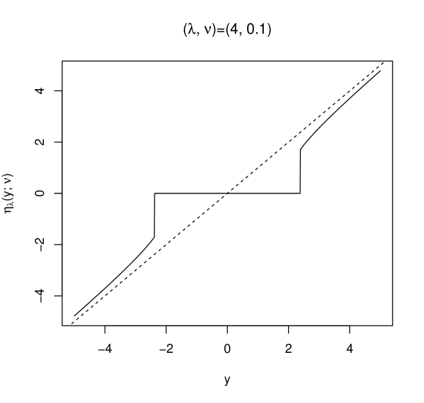
Figure 1: “Harder” thresholding function $\eta_{\lambda}(y;\nu)$ for $(\lambda,\nu)=(4,0.1)$. Dotted line: the identity function.

The thresholding effect of the penalty $P_{\nu}$ for the linear and ANN learners considered here is established by the following two theorems. Thresholding is due to the fact that $\rho_{\nu}(\theta)$ is even and has a strictly positive right-derivatives at zero. Indeed, one sees that $\lim_{\theta\rightarrow 0^{+}}\rho_{\nu}^{\prime}(\theta)=1$ (and $\lim_{\theta\rightarrow 0^{-}}\rho_{\nu}^{\prime}(\theta)=-1$) for all $0\leq\nu<1$, and $\lim_{\theta\rightarrow 0^{+}}\rho_{1}^{\prime}(\theta)=1/2$ (and $\lim_{\theta\rightarrow 0^{-}}\rho_{1}^{\prime}(\theta)=-1/2$). The singularity of $\rho_{\nu}(\theta)$ at zero with finite left- and right-derivatives creates a local minimum of the cost function in (9) provided $\lambda$ is large compared to the gradient of ${\cal L}_{n}$ at zero, as stated in the following theorem.

Theorem 2 (QUT compatibility of penalties $P_{\nu}$).

Consider (9) with a feature selection compatible MLP as described in Definition 1, with a loss ${\cal L}_{n}\in{\cal C}^{2}$ and with $P({\bm{\theta}}^{(1)})=P_{\nu}({\bm{\theta}}^{(1)})$ defined in (10). Then, for any fixed $\nu\in(0,1]$, the optimization problem has a local minimum at $\hat{\bm{\theta}}^{(1)}={\bf 0}$ if and only if $\lambda\geq\lambda_{0}^{\rm local}({\bf y},X)$ for some finite data-dependent value $\lambda_{0}({\bf y},X)$.

The proof of Theorem 2 is given in Appendix B. Ma et al. (2022) provide the closed form expression of the local zero-thresholding function $\lambda_{0}({\bf y},X)$ in regression and classification. Using the square root MSE loss $\mathcal{L}_{n}=\|\mathbf{y}-\mu_{\bm{\theta}}(X)\|_{2}$, the local zero-thresholding function is of the form

$$\lambda_{0}^{\rm local}({\bf y},X)=\pi_{l}\sigma^{\prime}(0)^{l-1}\frac{\|X^{\rm T}({\bf y}-\bar{\bf y}{\bf 1}_{n})\|_{\infty}}{\|{\bf y}-\bar{\bf y}{\bf 1}_{n}\|_{2}}.$$

In classification, using the cross-entropy loss $\mathcal{L}_{n}=\sum_{i=1}^{n}\mathbf{y}_{i}^{\top}\log\mu_{\theta}\left(\mathbf{x}_{i}\right)$, the local zero-thresholding function is of the form

$$\lambda_{0}^{\rm local}({\bf y},X)=\pi_{l}\sigma^{\prime}(0)^{l-1}\|X^{\rm T}({\bf y}-\bar{\bf y}{\bf 1}_{n})\|_{\infty}.$$

Here $\pi_{l}$ is a constant that depends on the product of the number of neurones in the layers. Since a linear learner of the form $\mu_{(\bm{\theta}^{(1)},\bm{\theta}^{(2)})}(\mathbf{x})=c+\bm{\theta}^{\top}\mathbf{x}$, where $(\bm{\theta}^{(1)},\bm{\theta}^{(2)})=(\bm{\theta},c)$, is a specific case of a feature-selection-compatible MLP, the theorem is similarly applicable. This allows us to express the local zero-thresholding function as $\lambda_{0}^{\text{local}}(\mathbf{y},X)=\frac{\|X^{\top}(\mathbf{y}-\bar{\bf y}\mathbf{1}_{n})\|_{\infty}}{\|\mathbf{y}-\bar{\bf y}\mathbf{1}_{n}\|_{2}}$ for regression and $\lambda_{0}^{\text{local}}(\mathbf{y},X)=\|X^{\top}(\mathbf{y}-\bar{\bf y}\mathbf{1}_{n})\|_{\infty}$ for classification.

This theorem translates to the possibility of choosing $\lambda$ with the QUT principle for the two learners considered and for our class of sparsity inducing penalties $P_{\nu}$. One expects a better phase transition for the probability of recovering the relavant features with the new penalty when $\nu$ is close to zero.

2.5 Optimization

Because of the non-differentiable penalty term of the cost function (9) to fit harderLASSO to the data, a gradient descent-based algorithm like Adam cannot be employed as such, but must be combined with an algorithm specifically designed for dealing with a sparsity inducing penalty like ISTA (Beck and Teboulle, 2009). Applying an ISTA step to minimize an optimization problem of the form $f(\theta)+g(\theta)$ requires solving

$$\min_{\bm{\theta}\in\mathbb{R}^{\gamma}}\frac{1}{2\delta_{(k)}}\left\|\left(\bm{\theta}_{(k)}-\delta_{(k)}\nabla f\left(\bm{\theta}_{(k)}\right)\right)-\bm{\theta}\right\|_{2}^{2}+g\left(\bm{\theta}_{(k)}\right)$$ (14)

at each iteration to move from the current iterate $\bm{\theta}_{(k)}$ to $\bm{\theta}_{(k+1)}$, where $\delta_{(k)}$ is a step size (similar to a learning rate). In our case, $g$ plays the role of the nondifferentiable sparsity inducing penalty $g(\bm{\theta})=\lambda P_{\nu}\left(\bm{\theta}^{(1)}\right)$ given in (10). The multivariate optimization (14) is separable and amounts to solving $\gamma=\sum_{k=1}^{l}p_{k+1}(p_{k}+1)$ univariate problems, either least squares problems for $\bm{\theta}^{(2)}$ or the univariate problems of Theorem 1 for $\bm{\theta}^{(1)}$.

Some key technicalities remain to be discussed regarding the initial values of the iterative algorithm, the choice of $(\lambda,\nu)$ and the learning rate $\delta_{(k)}$. Iterative algorithms require initial values. For harderLASSO ANN, the initial $\bm{\theta}_{(0)}^{(2)}$ is sampled from a standard Gaussian (since weights of layer 2 and above are normalized), and the weights of the first layer as well as all biases $\bm{\theta}_{(0)}^{(1)}$ are a sample from $\mathrm{N}\left(\mathbf{0},\sigma_{0}^{2}I_{\gamma_{1}}\right)$ with $\sigma_{0}^{2}=\operatorname{Var}(\mathbf{Y})$; the motivation for the variance $\sigma_{0}^{2}$ is that, for a linear model with a single needle, say $\mathbf{x}_{j}$, the coefficients should be of the order of $\operatorname{Var}(\mathbf{Y})$ since $\operatorname{Var}(\mathbf{Y})=\theta_{j}^{2}\operatorname{Var}(\mathbf{x}_{j})+\sigma^{2}$ and the columns of the input matrix are rescaled to variance $\operatorname{Var}(\mathbf{x}_{j})=1$.

While the ultimate goal is to solve (9) for $(\lambda,\nu)=\left(\lambda_{\alpha}^{\text{QUT }},0.1\right)$, we take the conservative approach of solving for a sequence of $(\lambda,\nu)$ ’s to prevent falling in a poor local minima, in the spirit of simulated annealing. Ma et al. (2022) proposed solving the cost function (9) for a linear and ANN models using an increasing sequence of $\lambda$ ’s tending to $\lambda=\lambda_{\alpha}^{\text{QUT }}$, namely $\lambda_{k}=\exp{(k-1)}/(1+\exp{(k-1)})\lambda_{\alpha}^{\text{QUT }}$ for $k\in\{0,\ldots,5,+\infty\}$. Taking as initial parameter values the solution corresponding to the previouc $\lambda_{k}$ leads to a sequence of sparser approximating solutions until solving for $\lambda_{\alpha}^{\text{QUT }}$ at the last step. This gradual increase helps mitigate the risk of falling into a poor local minima due to overly aggressive thresholding early in the process. Similarly we propose solving (9) using an increasing sequence of $(\lambda,\nu)$ pairs, converging to $\left(\lambda_{\alpha}^{\text{QUT }},0.1\right)$. The sequence for $\lambda$ remains as previously defined, while $\nu$ takes on values from the set $\{1,0.7,0.4,0.3,0.2,0.1\}$.

During the training with intermediate $(\lambda_{k},\nu_{k})$ pairs, we employ the Adam optimizer with an initial learning rate of $0.01$, while keeping the remaining optimizer parameters at their default settings. During training, the loss is monitored, and the learning rate is reduced by a factor of $0.5$ if an increase in loss is detected. In the final training phase, only the penalized parameters are updated. Due to the differing characteristics of the weights in the first layer and the biases, a block coordinate relaxation approach is adopted (Tseng, 2001; Sardy et al., 2000). Specifically, blocks are updated successively: first, the biases $(\mathbf{b}_{1},\ldots,\mathbf{b}_{l-1})$ are updated, followed by the first layer weights $W_{1}$, with each block solved using ISTA. A line search determines the step size for each block, after which momentum is applied to the updates. Each training phase is concluded when the relative improvement in the cost falls below a small threshold.

After completing all training phases, we can reduce the matrix $\hat{W}_{1}$ to $\hat{W}_{1}\in\mathbb{R}^{\tilde{p}_{2}\times s}$, where $s$ represent the number of selected features by the model. This is done by removing any neurons that consist entirely of zeros, resulting from the regularization applied to the matrix $W_{1}$. This adjustment impacts the subsequent layer’s weight matrix, so that $\hat{W}_{2}^{\circ}$ is now reshaped to $\hat{W}_{2}^{\circ}\in\mathbb{R}^{p_{3}\times\tilde{p}_{2}}$, where $\tilde{p}_{2}$ reflects the reduced number of active neurons. A final training phase without regularization is then applied to the reduced model, using the Adam optimizer to refine predictions and ensure optimal performance.

The optimization scheme is flexible and can be adapted as needed; it is not bound to a single approach. One could also start with a short training phase without regularization. In the case of basic LASSO, the scheme is implemented using a fixed parameter $\nu=1$ alongside the soft-thresholding operator to solve ISTA.

3 Monte Carlo simulation with regression task

We examine the performance of harderLASSO linear and artificial neural network by comparing them to various state-of-the-art models on the regression task that consists in predicting an output scalar $y$ from an input vector ${\bf x}$. The seven learners under consideration, all trained on the same datasets, are summarized in Table 1. All the LASSO-based methods, except LassoNet, use the square-root $\ell_{2}$-loss and select the penalty parameter $\lambda$ with the quantile universal rule (Giacobino et al., 2017b). Once $\lambda^{\rm QUT}$ value is calculated, the models are trained using the same $\lambda_{k}$ sequence as described in Section 2.5. LassoNet is a different neural network framework that achieves feature selection by adding a skip layer and integrating feature selection directly into the objective function; we select the tuning parameters of LassoNet using the built-in 10-fold cross-validation. Random Forest is based on the sklearn package with a configuration of 100 trees. The XGBoost learner is based on the xgboost Python package with default parameter settings. Given that both Random Forest and XGBoost primarily generate feature rankings rather than explicitly selecting features, we apply the Boruta algorithm to identify the most relevant features (Kursa et al., 2010). After determining the selected features using Boruta, we retrain the models on the selected subset: so random forest and XGBoost are two step methods here. If not stated otherwise, all neural network based models use one hidden layer of size $p_{2}=20$.

	Model	Description
	Linear
	harderLASSO linear	Square-root $\ell_{2}$-loss and near hard thresholding
	LASSO linear	Square-root $\ell_{2}$-loss and $\ell_{1}$ penalty (Belloni et al., 2011)
	ANN
0.	harderLASSO ANN	Same as above
1.	LASSO ANN	Same as above (Ma et al., 2022)
2.	LassoNet	$\ell_{2}$-loss with mixed penalties (Lemhadri et al., 2021)
	Ensemble learners
3.	Random Forest (RF)	Average of CART (Breiman, 2001)
4.	XGBoost	Extreme Gradient Boosting (Chen and Guestrin, 2016)

Table 1: Summary of models and learners considered.

To investigate the ability of the seven learners to select the correct features and to generalize, we consider $s$-sparse regression problems in the sense that out of the $p$ inputs (the haystack), only $s$ of them carry predictive information (the needles). We call ${\cal S}^{*}=\{j\in{\mathbb{R}}^{p}:\ x_{j}\mbox{ has some predictive information}\}$ the support of the regression, and $\hat{\cal S}$ is the estimated support. The regression is $s$-sparse when $|{\cal S}^{*}|=s$. To measure the quality of the seven learners to find a good association $\mu(\cdot)$ between input and output, we consider three criteria: the probability of exact support recovery (4), the $F_{1}$-score (5) and the generalization measured by the empirical $L_{2}$ distance between the true association $\mu$ and the estimated one $\hat{\mu}$,

$$\hat{L}_{2}=\frac{1}{n^{\prime}}\sum_{i^{\prime}=1}^{n^{\prime}}(\hat{\mu}({\bf x}_{i^{\prime}})-\mu({\bf x}_{i^{\prime}}))^{2},$$ (15)

where the ${\bf x}_{i^{\prime}}$’s are sampled from the same distribution as the ${\bf x}_{i}$’s of the training set and $n^{\prime}=1000$. In other words, $\hat{L}_{2}$ is an estimate of $d_{L_{2}}(\hat{\mu},\mu)=\int_{\mathbb{R}^{p_{1}}}(\hat{\mu}({\bf x})-\mu({\bf x}))^{2}f_{X}({\bf x})d{\bf x}$, where $f_{X}$ is the density function of the inputs. Since the training sets are generated from a known $s$-sparse model that we define below, the true support ${\cal S}^{*}$ and the true association $\mu(\cdot)$ are known, so all three criteria can be evaluated.

To simulate data sets of sample size $n$, we simulate a single $n\times p$ input matrix (the haystack), where the entries of $X$ are i.i.d. sampled from a standard Gaussian distribution. From that $X$ matrix, $m$ random $n\times s$ submatrices of needles $X_{n,s}^{(k)}$ for $k=1,\ldots,m$ are created by selecting $s$ random columns in $X$. Given an association $\mu$ from ${\mathbb{R}}^{s}$ to ${\mathbb{R}}$, then $m$ random training sets $\{(X_{n,s}^{(k)},{\bf y}^{(k)})\}_{k=1,\ldots,m}$ are simulated according to

$${\bf y}^{(k)}=\mu(X_{n,s}^{(k)})+{\bf e}^{(k)},$$

where $\mu$ acts row-wise on $X_{n,s}^{(k)}$ and ${\bf e}^{(k)}$ are i.i.d. sampled from a standard Gaussian distribution. In the next three sections we consider three associations $\mu$ between inputs and output: a linear and two nonlinear ones.

3.1 Zero hidden layer for linearity

For a linear simulation with $(n,p)=(70,250)$, $s\in\{0,1,\ldots,30\}$, we set $\mu(X_{s})=X_{s}{\bm{\beta}}$ with each entry of ${\bm{\beta}}\in{\mathbb{R}}^{s}$ set to 3. The pair $(n,p)$ is fixed and $s\in\{0,1,\ldots,30\}$ increases to observe a phase transition. Figure 2 summarizes the results of the linear Monte-Carlo simulations with $m=100$ runs: clearly, harderLASSO wins over all criteria and the harder/non convex penalty considerably improves over the convex LASSO penalty thanks to less shrinkage of the non-zero weights in the first layer. Of course, the linear model remains the best option in this case. Our learners are the only one to have a clear phase transition. This is achieved thanks to a good selection of a single penalty parameter $\lambda$ with the quantile universal rule and thanks to a performant optimization numerical scheme with a grid of $(\lambda,\nu)$’s slowly cooling to $(\lambda^{\rm QUT}_{\alpha},0.1)$, in the spirit of simulated annealing.

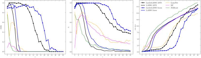
Figure 2: Linear Monte-Carlo simulation results. Left plot: estimated probability of exact support recovery. Center plot: $F_{1}$ score. Right plot: square root $\hat{L}_{2}$.

3.2 One hidden layer for simple nonlinearity

For a simple nonlinear simulation with $(n,p)=(500,50)$, $s=2h$ with $h\in\{0,1,\ldots,10\}$, we set $\mu({\bf u})=\sum_{i=1}^{h}\beta\cdot|u_{2i}-u_{2i-1}|$ with $\beta=10$ and ${\bf u}\in{\mathbb{R}}^{s}$. The pair $(n,p)$ is fixed and $s\in\{0,1,\ldots,20\}$ increases to observe a phase transition. Figure 3 summarizes the results of the nonlinear Monte-Carlo simulations with $m=100$ runs: the same conclusion holds pointing to the superiority of harderLASSO over its competitors.

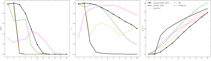
Figure 3: Nonlinear Monte-Carlo simulation results. Left plot: estimated probability of exact support recovery. Center plot: $F_{1}$ score. Right plot: square root $\hat{L}_{2}$.

3.3 Deeper ANN for a more complex nonlinearity

For an increasing sample size $n$ and $s=4$ fixed, we consider ANNs with 1, 2 and 3 hidden layers to empirically investigate their respective abilities to create a phase transition not only in the probability of retrieving the four features but also in unveiling the complex nonlinearity of the $s$-sparse function, defined as:

$$\mu(\mathbf{x})=\big{\lvert}10\cdot\lvert x_{2}-x_{1}\rvert-10\cdot\lvert x_{4}-x_{3}\rvert\big{\rvert}.$$ (16)

This nonlinear association is approximated by a sparse two hidden layer ANN employing the ReLU activation function and with $\bm{b}_{1}=\bm{0}_{\tilde{p}_{2}}$, $\bm{b}_{2}=\bm{0}_{p_{3}}$, $\bm{w}_{3}=(1,1)$, $c=0$ and,

$$W_{1}=\begin{pmatrix}1&-1&0&0\\ -1&1&0&0\\ 0&0&1&-1\\ 0&0&-1&1\\ \end{pmatrix},\quad W_{2}=\begin{pmatrix}10&10&-10&-10\\ -10&-10&10&10\\ \end{pmatrix}.$$

Here, $W_{1}$ is already in its reduced form, the matrices $W_{2}$ and $\bm{w}_{3}$ can be arbitrarily extended with zeros to match the required dimensions $p_{3}$. Since our method involves row-wise normalization of $W_{2}$, we do not expect our model to exactly replicate the proposed $W_{2}$ matrix. Instead, the coefficients may be distributed differently among the various weights due to the normalization process, effectively splitting the original coefficients across multiple connections within the network.

Although we have described the neural network using the ReLU activation function for the sake of generality, recall that in Definition 1 we specified that ReLU cannot be used within our neural networks. This difference is acceptable because employing a different activation function—such as a shifted version of ReLU or the ELU with $\alpha=1$—would result in the same network structure, albeit with different bias values. The key takeaway is that accurately representing the function requires two hidden layers.

Because a single hidden layer ANN is insufficient to accurately approximate this association, we expect poor generalization; yet, exact support recovery may be high, which is not paradoxical. Indeed a fitted model may employ the correct needles, but in a suboptimal way. In contrast, a two hidden layer ANN should yield good exact support recovery and generalization, effectively capturing the complex nonlinear relationships involved. While a three hidden layer ANN should also fit the data well, one may expect a need of a larger sample size $n$ to match the performance of the two hidden layer ANN: indeed, the additional flexibility of adding another layer and more parameters has a cost.

We investigate the performance of ANNs with 1, 2 and 3 hidden layers (with $p_{2}=20$, $(p_{2},p_{3})=(20,10)$ and $(p_{2},p_{3},p_{4})=(20,10,5)$) to fit the nonlinear association (16) using a Monte Carlo simulation. Here we choose $p_{1}=50$ inputs and generate a single $6500\times p_{1}$ input Gaussian matrix and selects its first $n$ rows to create data sets of size $n$ with increasing sample size ranging from 100 to 6500 by steps of 100. Then we simulate $m=50$ submatrices $X_{n,s}^{(k)}$ and generate $m$ training sets with (16), as in the previous simulation.

Figure 4 displays the Monte Carlo results. We observe that the 1 hidden layer ANN (blue) has a rapidly growing PESR (left), but its corresponding predictive performance (right) plateaus at a high level since it does not have enough flexibility to match the full nonlinearity of the association. The 2 hidden layer ANN (green) also has a rapid PESR increase, though less early, and its predictive performance does not plateau but keeps on improving. The 3 hidden layer ANN (yellow) has an even slower PESR increase and its predictive performance nearly matches that of the 2 hidden layer ANN when $n$ gets large.

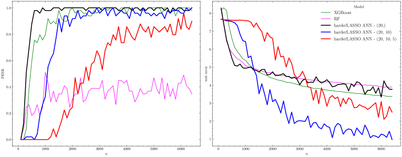
Figure 4: Simulation results based on $m=50$ Monte Carlo runs as a function of sample size $n$ for three ANNs with 2, 3 and 4 layers. Left plot: estimated probability of exact support recovery. Right plot: square root $\hat{L}_{2}$ on a test set of size $1000\times 50$.

4 Applications with classification task

We apply five learners on several “real-world” datasets detailed in Table 2, which lists the number of instances $n$, number of features $p$ and the number of classes $m$. To quantify the accuracy relative to the number of needles identified by the learners, we average the models performance over 50 resamplings to ensure stability and reliability in our findings. In each resampling iteration, the dataset is randomly partitioned, with two-thirds of the data allocated for training and one-third reserved for testing. When missing values are present, mean imputation is employed. If separate training, testing, and validation sets are provided, these sets are concatenated to form the dataset before partitioning.

Dataset	Type	n	p	m	Source
Biological Data
obesity	Medical	2111	16	7	UCI
dry bean	Biological	13611	16	7	UCI
aids	Medical	2139	23	2	UCI
dna	Biological	3186	180	3	OpenMl
Toy/Benchmark Data
iris	Benchmark	150	4	3	Python sklearn
breast	Benchmark	569	30	2	Python sklearn
wine	Benchmark	178	13	3	Python sklearn
Other Data
USPS	Images	9298	257	10	Kaggle
mail	Spam recognition	4601	57	2	UCI
statlog	Climate and Environment	6435	36	7	UCI
titanic	Survival Analysis	714	8	2	Kaggle
chess	Games	3196	35	2	UCI

Table 2: Datasets used for classification with some key characteristics.

Figure 5: Trade-off between feature selection efficiency and accuracy for five learners.

Figure 5 summarizes the results of our analysis (of which Table 3 in Appendix C reports the summary statistics). Each dataset is represented by a unique color, and the same indices as in Table 1 are used for the different models. The larger black digits indicate the average sparsity level and accuracy of all the data sets for each of the five learners. Like in regression, we observe in classification that harderLASSO behaves better than LASSO with more accuracy and less selected features. The accuracy of harderLASSO is almost as high as the other learners, yet with much less selected features. Among all five learners, harderLASSO is clearly the most frugal of all. Appendix D plots the distribution of selected features between the fifty training sets for three data sets to illustrate the stability of the method.

5 Conclusion

The harderLASSO ANN learner adjusts to the data’s sparsity level, enhancing the selection of important features while maintaining strong generalization. Not being an ensemble method, and being driven by a single regularization parameter which does not require a validation set for its selection, harderLASSO performs remarkably well compared to the current best learners as it competes for accuracy with a much smaller amount of selected relevant inputs.

One of the most remarkable aspects of harderLASSO ANN is its user-friendliness: it is as simple as “click start and wait,” with the model autonomously computing all necessary parameters. This makes it highly accessible, especially for users who want powerful results with minimal manual setup. Potential upgrades to the model includes improved optimization techniques, such as exploring the parameter space with different initialization points, different optimization schemes and learning rates. The phase transition curves provided here serve as a lower bound benchmark to test future optimization schemes: improvement means either higher phase transition or lower CPU time, or both.

The methods presented here extend beyond current applications and can be generalized for diverse objectives. As long as the penalty is QUT-compatible and a closed-form expression of $\lambda^{\rm QUT}$ exists, this optimization framework can support various tasks, such as survival analysis, among other future applications.

6 Reproducible research

The codes used to create the figures and tables are available at https://github.com/VcMaxouuu/AnnLasso.

7 Acknowledgement

We thank Dr. Thomas Kerdreux for his helpful comments. This work was partially supported by the Swiss National Science Foundation grant 200021E_213166 and the Academic Rising Star Project No. 2024-YJRC-LXY-005 of the National University of Defense and Technology, China.

Appendix A Proof of Threorem 1

Call $f(\theta;y)$ the cost function (12) for given $\lambda>0$ and $\nu\in(0,1]$. We consider the case $y>0$. To create two local minima with the same cost value (one at zero and the other at some positive value $\theta$) for some high enough value $y$, we want to solve over $y>0$ and $\theta>0$

$$\left\{\begin{array}[]{l}f(0;y)=f(\theta;y)\\ f^{\prime}(\theta;y)=0\end{array}\right. \Leftrightarrow \left\{\begin{array}[]{l}y^{2}=(\theta-y)^{2}+2\lambda\frac{\theta}{1+\theta^{1-\nu}}\\ \theta-y+\lambda\frac{1+\nu\theta^{1-\nu}}{(1+\theta^{1-\nu})^{2}}=0\end{array}\right.$$

$$\Leftrightarrow \left\{\begin{array}[]{l}y=\theta/2+\lambda\frac{1}{1+\theta^{1-\nu}}\\ y=\theta+\lambda\frac{1+\nu\theta^{1-\nu}}{(1+\theta^{1-\nu})^{2}}\end{array}\right.$$

$$\Leftrightarrow \left\{\begin{array}[]{l}\theta^{2-\nu}+2\theta+\theta^{\nu}+2\lambda(\nu-1)=0\\ y=\theta/2+\lambda\frac{1}{1+\theta^{1-\nu}}\end{array}\right.,$$

where the threshold is $\varphi(\lambda,\nu):=y$ and the jump is $\kappa(\lambda,\nu):=\theta$.

To numerically solve the first equation of the system over $\theta>0$ for $\nu\in(0,1]$ and $\lambda>0$ fixed, note that

$$\theta^{2-\nu}+2\theta+\theta^{\nu}+2\lambda(\nu-1)=0$$

$$\Leftrightarrow~{}~{}~{}~{}~{}\left(\theta^{1-\frac{\nu}{2}}+\theta^{\frac{\nu}{2}}\right)^{2}=2\lambda(1-\nu)$$

$$\Leftrightarrow~{}~{}~{}~{}~{}\theta^{1-\frac{\nu}{2}}+\theta^{\frac{\nu}{2}}=\sqrt{2\lambda(1-\nu)}.$$

And since $\theta^{1-\frac{\nu}{2}}+\theta^{\frac{\nu}{2}}\geq 2\sqrt{\theta^{1-\frac{\nu}{2}}\cdot\theta^{\frac{\nu}{2}}}=2\sqrt{\theta}$ (inequality of arithmetic and geometric means), we must have that $\theta\in\left(0,\frac{\lambda(1-\nu)}{2}\right]$.

Appendix B Proof of Theorem 2

Let ${\bm{\theta}}^{(1)}$ be the parameter with $\lVert{\bm{\theta}}^{(1)}\rVert_{1}=1$ and ${\bf c}_{1}\in\mathbb{R}^{r}$ be any vector with $\lVert{\bf c}_{1}\rVert_{1}=1$. Let ${{\bm{\theta}}^{\epsilon}}=(\epsilon{\bm{\theta}}^{(1)},W_{2},\ldots,W_{l},\hat{\bf c}+\epsilon{\bf c}_{1})$ for any $\tilde{\bm{\theta}}=(W_{2},\ldots,W_{l})$. Since the loss function ${\cal L}_{n}$ is twice differentiable with respect to ${{\bm{\theta}}}^{(1)}$ around ${\bm{\theta}}^{0}=({\bf 0},W_{2},\ldots,W_{l},\hat{\bf c})$, applying Taylor’s theorem we have

$$|{\cal L}_{n}({\cal Y},\mu_{{\bm{\theta}}^{\epsilon}}({\cal X}))-{\cal L}_{n}({\cal Y},\mu_{{\bm{\theta}}^{0}}({\cal X}))| = |\nabla_{{\bm{\theta}}_{1}}{\cal L}_{n}({\cal Y},\mu_{{\bm{\theta}}^{0}}(x))(\epsilon{\bm{\theta}}_{1})+\nabla_{{\bf c}_{1}}{\cal L}_{n}({\cal Y},\mu_{{\bm{\theta}}^{0}}({\cal X}))(\epsilon{\bf c}_{1})$$

$$+o(\epsilon^{2}\lVert{{\bm{\theta}}}^{(1)}\rVert_{1})+o(\epsilon^{2}\lVert{\bf c}_{1}\rVert_{1})|$$

$$= |\epsilon g_{0}({\cal Y},{\cal X},{\bm{\theta}}^{0}){{\bm{\theta}}}^{(1)}+0+o(\epsilon^{2})|$$

$$\leq |\epsilon|\lVert g_{0}({\cal Y},{\cal X},{\bm{\theta}}^{0})\rVert_{\infty}+o(\epsilon^{2}).$$

Therefore we get ${\cal L}_{n}({\cal Y},\mu_{{\bm{\theta}}^{\epsilon}}({\cal X}))\geq{\cal L}_{n}({\cal Y},\mu_{{\bm{\theta}}^{0}}({\cal X}))-|\epsilon|\lVert g_{0}({\cal Y},{\cal X},{\bm{\theta}}^{0})\rVert_{\infty}+o(\epsilon^{2}).$ If we assume that $(\lambda-\sup_{\tilde{\bm{\theta}}}\lVert g_{0}({\cal Y},{\cal X},{\bm{\theta}}^{0})\rVert_{\infty})>C>0$, it follows that the regularized loss satisfies

$${\cal L}_{n}({\cal Y},\mu_{{\bm{\theta}}^{\epsilon}}({\cal X}))+\lambda P_{\nu}(\epsilon{{\bm{\theta}}}^{(1)}) \geq{\cal L}_{n}({\cal Y},\mu_{{\bm{\theta}}^{0}}({\cal X}))-|\epsilon|\lVert g_{0}({\cal Y},{\cal X},{\bm{\theta}}^{0})\rVert_{\infty}+\lambda P_{\nu}(\epsilon{{\bm{\theta}}}^{(1)})+o(\epsilon^{2})$$

$$={\cal L}_{n}({\cal Y},\mu_{{\bm{\theta}}^{0}}({\cal X}))-|\epsilon|\lVert g_{0}({\cal Y},{\cal X},{\bm{\theta}}^{0})\rVert_{\infty}$$

$$\ \ +\lambda\sum_{j}|\epsilon\theta_{1j}^{(1)}|\frac{1}{1+|\epsilon\theta_{1j}^{(1)}|^{1-\nu}}+o(\epsilon^{2})$$

$$={\cal L}_{n}({\cal Y},\mu_{{\bm{\theta}}^{0}}({\cal X}))-|\epsilon|\lVert g_{0}({\cal Y},{\cal X},{\bm{\theta}}^{0})\rVert_{\infty}$$

$$+\lambda\sum_{j}\left[|\epsilon\theta_{1j}^{(1)}|-|\epsilon\theta_{1j}^{(1)}|^{2-\nu}+|\epsilon\theta_{1j}^{(1)}|^{3-2\nu}+o(|\epsilon\theta_{1j}^{(1)}|^{3-2\nu})\right]+o(\epsilon^{2})$$

$$={\cal L}_{n}({\cal Y},\mu_{{\bm{\theta}}^{0}}({\cal X}))-|\epsilon|\lVert g_{0}({\cal Y},{\cal X},{\bm{\theta}}^{0})\rVert_{\infty}+\lambda|\epsilon|\|{\bm{\theta}}^{(1)}\|_{1}$$

$$\ \ +\lambda\sum_{j}O(|\epsilon\theta_{1j}^{(1)}|^{2-\nu})+o(\epsilon^{2})$$

$$>{\cal L}_{n}({\cal Y},\mu_{{\bm{\theta}}^{0}}({\cal X}))+|\epsilon|C+\lambda\sum_{j}O(|\epsilon\theta_{1j}^{(1)}|^{2-\nu})+o(\epsilon^{2})$$

$$>{\cal L}_{n}({\cal Y},\mu_{{\bm{\theta}}^{0}}({\cal X}))\quad\text{for $|\epsilon|$ small enough.}$$

Thus the cost function with our choice of $\lambda$ has a local minimum at ${\bm{\theta}}^{0}$. Since layers $2$ to $l$ have normalized weights, the supremum $\sup_{\tilde{\bm{\theta}}}\lVert g_{0}({\cal Y},{\cal X},{\bm{\theta}}^{0})\rVert_{\infty}):=\lambda_{0}({\bf y},X)$ is finite, which defines the zero-thresholding function $\lambda_{0}({\bf y},X)$. Consequently the zero-thresholding functions for ANN with the new penalty are the same as those derived by Ma et al. (2022) in regression and classification, regardless of the value of $\nu\in(0,1]$.

Appendix C Summary of classifcation data

Table 3 summarizes the Monte Carlo study corresponding to Figure 5 for the real data listed in 2.

	ANN
Dataset	harderLASSO	LASSO	LassoNet	RF	XGBoost
obesity	(3.0, 0.89)	(5.86, 0.62)	(15.68, 0.81)	(11.98, 0.95)	(12.28, 0.97)
dry bean	(6.0, 0.91)	(7.0, 0.9)	(15.98, 0.92)	(16.0, 0.92)	(13.0, 0.93)
aids	(3.68, 0.88)	(3.82, 0.81)	(18.82, 0.86)	(5.12, 0.85)	(6.42, 0.88)
dna	(9.04, 0.92)	(12.22, 0.9)	(148.44, 0.94)	(83.06, 0.96)	(18.64, 0.95)
iris	(1.88, 0.95)	(1.88, 0.8)	(3.1, 0.93)	(4.0, 0.95)	(2.04, 0.95)
breast	(2.22, 0.94)	(4.1, 0.95)	(25.88, 0.96)	(22.9, 0.96)	(9.68, 0.96)
wine	(2.3, 0.9)	(4.94, 0.94)	(10.72, 0.97)	(13.0, 0.98)	(7.02, 0.96)
USPS	(14.8, 0.83)	(50.96, 0.82)	(255.26, 0.93)	(208.82, 0.96)	(108.62, 0.96)
mail	(15.88, 0.9)	(25.46, 0.88)	(56.5, 0.94)	(19.66, 0.95)	(23.24, 0.95)
statlog	(5.08, 0.84)	(22.94, 0.8)	(36.0, 0.88)	(36.0, 0.91)	(35.84, 0.91
titanic	(2.38, 0.78)	(2.52, 0.78)	(5.9, 0.79)	(3.96, 0.8)	(3.68, 0.78)
chess	(7.22, 0.94)	(8.52, 0.94)	(33.4, 0.97)	(14.52, 0.97)	(17.54, 0.98)

Table 3: Results on the classification datasets. The first value is the number of selected features and the second value is the accuracy on the testing set averaged over 50 resamplings.

Appendix D Feature selection example

Figure 6 reports the feature importances of harderLASSO ANN for the Titanic, Mail, and Breast datasets.

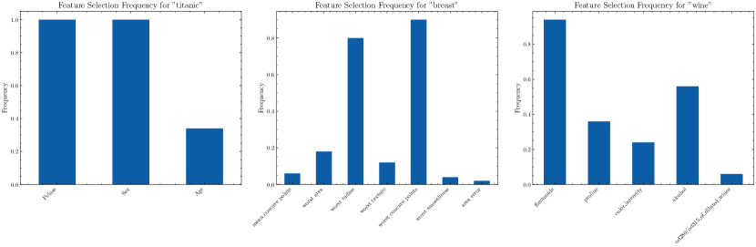
Figure 6: Feature selection frequencies identified by harderLASSO ANN for the Titanic, Mail, and Breast datasets, estimated over the 50 random trainings.

References

- Bach et al. [2011] F. Bach, R. Jenatton, J. Mairal, and G. Obozinski. Optimization with sparsity-inducing penalties. Foundations and Trends in Machine Learning, 4(1):1–106, 2011.
- Beck and Teboulle [2009] A. Beck and M. Teboulle. A fast iterative shrinkage-thresholding algorithm for linear inverse problems. SIAM Journal on Imaging Sciences, 2:183–202, 2009.
- Belloni et al. [2011] A. Belloni, V. Chernozhukov, and L. Wang. Square-root lasso: pivotal recovery of sparse signals via conic programming. Biometrika, 98(4):791–806, 2011.
- Breiman [2001] L. Breiman. Random forests. Machine Learning, 45(1):5–32, 2001.
- Bühlmann and van de Geer [2011] P. Bühlmann and S. van de Geer. Statistics for High-Dimensional Data: Methods, Theory and Applications. Springer, Heidelberg, 2011.
- Candès and Romberg [2007] E. Candès and J. Romberg. Sparsity and incoherence in compressive sampling. Inverse Problems, 23(3):969–985, 2007.
- Chartrand [2007] R. Chartrand. Exact reconstruction of sparse signals via nonconvex minimization. IEEE Signal Processing Letters, 14(10):707–710, 2007.
- Chartrand and Yin [2008] R. Chartrand and W. Yin. Iteratively reweighted algorithms for compressive sensing. pages 3869–3872, 2008.
- Chen et al. [1999] S. S. Chen, D. L. Donoho, and M. A. Saunders. Atomic decomposition by basis pursuit. SIAM Journal on Scientific Computing, 20(1):33–61, 1999.
- Chen and Guestrin [2016] T. Chen and C. Guestrin. Xgboost: A scalable tree boosting system. In Proceedings of the 22nd ACM SIGKDD International Conference on Knowledge Discovery and Data Mining, volume 11, page 785–794. ACM, August 2016.
- Descloux and Sardy [2021] P. Descloux and S. Sardy. Model selection with lasso-zero: adding straw in the haystack to better find needles. Journal of Computational and Graphical Statistics, 30(3):530–543, 2021.
- Donoho [2006] D. L. Donoho. Compressed sensing. IEEE Transactions on Information Theory, 52:1289–1306, 2006.
- Donoho and Johnstone [1994] D. L. Donoho and I. M. Johnstone. Ideal spatial adaptation by wavelet shrinkage. Biometrika, 81(3):425–455, 1994.
- Donoho et al. [1995] D. L. Donoho, I. M. Johnstone, G. Kerkyacharian, and D. Picard. Wavelet shrinkage: asymptopia? Journal of the Royal Statistical Society: Series B, 57(2):301–369, 1995.
- Giacobino et al. [2017a] C. Giacobino, S. Sardy, J. Diaz Rodriguez, and N. Hengardner. Quantile universal threshold. Electronic Journal of Statistics, 11(2):4701–4722, 2017a.
- Giacobino et al. [2017b] C. Giacobino, S. Sardy, J. Diaz-Rodriguez, and N. Hengartner. Quantile universal threshold. Electron. J. Statist., 11(2):4701–4722, 2017b.
- Kursa et al. [2010] M. Kursa, A. Jankowski, and W. Rudnicki. Boruta - a system for feature selection. Fundam. Inform., 101:271–285, 01 2010.
- Lemhadri et al. [2021] I. Lemhadri, F. Ruan, L. Abraham, and R. Tibshirani. Lassonet: a neural network with feature sparsity. J. Mach. Learn. Res., 22(1), January 2021.
- Ma et al. [2022] X. Ma, S. Sardy, N. Hengartner, N. Bobenko, and Y. T. Lin. A phase transition for finding needles in nonlinear haystacks with lasso artificial neural networks. Statistics and Computing, 2022.
- Sardy [2009] S. Sardy. Adaptive posterior mode estimation of a sparse sequence for model selection. Scandinavian Journal of Statistics, 36(4):577–601, 2009.
- Sardy and Ma [2024] S. Sardy and X. Ma. Sparse additive models in high dimensions with wavelets. Scandinavian Journal of Statistics, 51(1):89–108, 2024.
- Sardy et al. [2000] S. Sardy, A. G. Bruce, and P. Tseng. Block coordinate relaxation methods for nonparametric wavelet denoising. Journal of Computational and Graphical Statistics, 9:361–379, 2000.
- Su et al. [2015] W. Su, M. Bogdan, and E. Candes. False discoveries occur early on the lasso path. The Annals of Statistics, 45:2133–2150, 11 2015.
- Tibshirani [1996] R. Tibshirani. Regression shrinkage and selection via the lasso. Journal of the Royal Statistical Society, Series B, 58(1):267–288, 1996.
- Tseng [2001] P. Tseng. Convergence of block coordinate descent method for nondifferentiable minimization. Journal of Optimization Theory and Applications, 109:475–494, 2001.
- Woodworth and Chartrand [2016] J. Woodworth and R. Chartrand. Compressed sensing recovery via nonconvex shrinkage penalties. Inverse Problems, 32(7):075004, May 2016. ISSN 1361-6420. doi: 10.1088/0266-5611/32/7/075004. URL http://dx.doi.org/10.1088/0266-5611/32/7/075004.
- Yuan and Lin [2006] M. Yuan and Y. Lin. Model selection and estimation in regression with grouped variables. Journal of the Royal Statistical Society, Series B, 68(1):49–67, 2006.