Gravitational waves and cosmic boundary

Abstract

Space-based gravitational wave detectors have the capability to detect signals from very high redshifts. It is interesting to know if such capability can be used to study the global structure of the cosmic space. In this paper, we focus on one particular question: if there exists a reflective cosmic boundary at the high redshift ($z>15$), is it possible to find it? We find that, with the current level of technology: 1) gravitational waves appear to be the only means with which that signatures from the cosmic boundary can possibly be detected; 2) a large variety of black holes, with masses roughly in the range ${\cal O}(10^{3}\sim 10^{6}){\rm~{}M_{\odot}}$, can be used for the task; 3) in the presumably rare but physically possible case that two merger events from the growth history of a massive black hole are detected coincidentally, a detector network like TianQin+LISA is essential in help improving the chance to determine the orientation of the cosmic boundary; 4) the possibility to prove or disprove the presence of the cosmic boundary largely depends on how likely one can detect multiple pairs of coincident gravitational wave events.

I Introduction

What is the size and topology of the three dimensional cosmic space? This is one basic question that still lacks an answer. The observable portion of the cosmic space is consistent with being flat Aghanim et al. (2020); Lahav and Liddle (2024). For a three dimensional flat space, there are 18 possible topologies, with the simplest being the infinitely large Euclidean space $\mathbb{R}^{3}$, and the simplest nontrivial case being the 3-torus, $T^{3}$, made from a rectangular prism with each pair of its opposite faces simply identified. All the 17 nontrivial topologies involve compact directions supporting closed geodesics that cannot be shrunk to a point continuously, and they all give raise to a multi-connected universe without a boundary. For a detailed description of Euclidean topologies relevant for cosmology, we refer to Eskilt et al. (2024).

Nontrivial cosmic topology can have nontrivial impact on the Cosmic Microwave Background (CMB). CMB photons we see today have been emitted from the last-scattering surface (LSS) at recombination. The LSS bounds the portion of the cosmic space that has been directly observed. One way to search for nontrivial topology is to look for the corresponding modification of the CMB spectrum Lachieze-Rey and Luminet (1995); Levin (2002). This method is model dependent and faces the difficulty of having unlimited possibilities on the choice of topologies and their parameters. Another method is to look for matched circles on the CMB sky Cornish et al. (1998). If the cosmic space has a nontrivial topology, such as $T^{3}$, an observer would see (assuming unlimited light power and waiting time) infinitely many copies of herself making up a three dimensional grid. Each grid point has a copy of the LSS to itself. If there is a compact direction smaller than the diameter of the LSS, then the LSSs of two nearby grid points will intersect each other. Since all grid points are in fact one of the same, the circle where the two nearby LSSs intersect will be seen by the observer as two circles located in opposite directions of the sky but with matched temperature variations. So far all matched circle searches have yielded null results de Oliveira-Costa et al. (2004); Cornish et al. (2004); Shapiro Key et al. (2007); Mota et al. (2010); Bielewicz and Banday (2011); Bielewicz et al. (2012); Vaudrevange et al. (2012); Aurich and Lustig (2013); Ade et al. (2014, 2016). Since different topologies and choices of parameters predict different patterns of matched circles, such null results mean differently for different topologies, with many still allowed to have a compact direction smaller than the diameter of the LSS Mihaylov et al. (2023); Akrami et al. (2024). However, the null results do exclude all closed and Earth (observer) passing geodesics that are topologically nontrivial and are shorter than the diameter of the LSS. So one is not expected to detect multiple images from a same astrophysical object due to nontrivial topology. Of course, this may change in the future when the size of the LSS has become large enough. This can be tested by observing distant galaxies, see zhi Fang and Sato (1983); Fagundes and Wichoski (1987); Roukema (1996); Lehoucq et al. (1996); Luminet and Roukema (1999); Fujii and Yoshii (2011, 2013); Roukema et al. (2014); Luminet (2016); Weatherley et al. (2003) and references therein.

The null results on matched circles also mean that there will be no observationally nontrivial signatures for individual gravitational wave (GW) events. But a flat cosmic space can have nontrivial global structures other than the topologies mentioned above. For example, all the 18 topologies mentioned above describe a cosmic space without boundaries, but one may as well consider a cosmic space with boundaries. The simplest example is the simply connected Euclidean space bounded from all directions. Such cosmic space is topologically equivalent to a 3-disk, $D^{3}$. For later convenience, we will refer to such model of the cosmic space the Bounded Cosmic Space (BCS) and its boundaries the Cosmic Boundary (CB). Some theoretical motivation for the BCS will be given in the next section.

There is no reason to believe that the size of the BCS is tied to that of the LSS. Instead, the former could be much larger than the latter. In this case, the BCS will not be relevant for observation unless part of the CB happens to be enclosed by the LSS (see Fig. 1 for an illustration). To be consistent with the CMB observations, the CB should be reflective. In this case, the CB acts like a mirror and evidence for the CB can be obtained if one can identify an astrophysical object together with its image in the CB. If the CB is close enough, one may try to observe it with electromagnetic telescopes. For example, the current most distant known galaxy has been found by JWST at a redshift $z\approx 14.3$ Carniani et al. (2024). If the CB is further away, one will need a method with even deeper spatial reach. Fortunately, the breakthrough in GW detection has greatly enhanced our capability to detect physics from the high redshifts. For example, GW detectors planned for the 2030s will not have much difficulty in reaching redshifts $z>15$ Seoane et al. (2013); Amaro-Seoane et al. (2017); Luo et al. (2016); Hu et al. (2017); Wang et al. (2019); Mei et al. (2021); Torres-Orjuela et al. (2024); Hu and Wu (2017); Evans et al. (2021); Maggiore et al. (2020); Bailes et al. (2021); Branchesi et al. (2023).

In this paper, we focus on using GW signals from massive black hole (MBH) systems to explore the possible presence of a reflective CB. Revealing the formation and growth history of MBHs is one of the most important scientific objectives of the upcoming space-based GW detectors Seoane et al. (2023); Wang et al. (2019). It is likely that a MBH can experience many mergers throughout its growth history Dayal et al. (2019); Pacucci and Loeb (2020); Piana et al. (2020); Liu and Inayoshi (2024). If a MBH is located close enough to the CB and has merger events at the right times, then a detector might be able to detect two merger events from the history of the same MBH, with the earlier signal taking the longer route that involves a reflection from the CB. Such pairs of coincident signals could be rare but are physically possible. If detected and confirmed, such signals will not only provide evidence for the existence of the CB, but will also offer valuable information on the growth history of the MBH. The purpose of this paper is to study such detection scenario in detail and to find the relevant parameter space for the MBHs.

The rest of the paper is organized as following. In section II, we present some theoretical motivation for the BCS and discuss the possible properties of the CB. In section III, we study the detection scenario and the relevant parameter space in detail. In section IV, we conclude with a short summary and discussion.

II The Bounded Cosmic Space and the cosmic boundary

The idea for a finite and bounded cosmic space can naturally arise from the perspective of emergent gravity (see Hu (2009); Sindoni (2012); Carlip (2014); Linnemann and Visser (2018) and references therein). In emergent gravity, various aspects of gravity, such as the spacetime manifold, the spacetime metric, and the dynamics of the spacetime metric, can all be emergent from some more fundamental construction, such as some fundamental particles (e.g., Hu (2009); Sindoni (2012)). Regardless of their detailed properties, a system of interacting particles are expected to collectively behave like a fluid at the macroscopic scale. This observation has been used to help understand the fluid/gravity correspondence Bhattacharyya et al. (2008); Rangamani (2009); Hubeny et al. (2012) based on the AdS/CFT correspondence Maldacena (1998). In the context of emergent gravity, however, this observation indicates the fluid/gravity equivalence Mei (2022, 2023):

• The existence of our cosmic space (the kind of cosmic space that is familiar to us) is due to the existence of some hidden fluid, and the properties of spacetime and gravity are determined by the properties of the hidden fluid and how it interacts with matter.

The hidden fluid is expected to exist on some more fundamental supporting structure, which we call the dry vacuum. Very much like a drop of water in the empty space, the hidden fluid is expected to occupy only a finite region of the dry vacuum. For the model considered in Mei (2022, 2023), the expansion of the universe is correlated to the decrease in the density of the hidden fluid, and the universe would be infinitely expanded if the density of the hidden fluid goes to zero. From the perspective of the dry vacuum, this indicates that the region without the hidden fluid is not traversable to everything that perceives a common expansion of our current universe. As a result, our cosmic space is confined to the region of the dry vacuum permeated by the hidden fluid, leading to the BCS. To help visualize the picture, one may use the fish tank as an analogy: the hidden fluid is like the water in the fish tank, everything that propagates in our cosmic space is like fish in the fish tank, and that one is not able to get beyond the CB is like fish cannot get away from the water.

Of course, the above motivation is helpful but is not crucial to the experimental search of the CB. Since there is no credible theory that can make convincing predictions on the global structure of the cosmic space, one may take the pragmatic point of view that, the presence (or not) of a CB is something that can only be answered with experimental observations.

For the properties of the CB, there is no reason to believe that the size of the BCS is similar to that of the LSS or that the shape of the BCS is simple and symmetric. For example, the BCS can be much larger than the LSS and its shape can be distorted. Of course, in order for the CB to be relevant for observations, we need to focus on the possibility that the LSS happens to be located to a side of the BCS and intersects with part of the CB, as illustrated in Fig. 1 (Left). To keep the discussion simple, we will assume that the portion of the CB that is inside the LSS is flat. Fig. 1 (Right) is a zoom-in on the LSS. The plane of the figure goes through the observer O in the solar system and is perpendicular to the CB. The CB cuts off part of the LSS and everything to the right of the CB in fact does not exist. The dashed curve is at the mirror position of the dotted curve. If the CB is fully absorptive, then there would be a dark patch on the CMB sky. Since this has not been observed, we assume that the CB is fully reflective for both light and GWs. In this case, the dashed curve replaces the dotted curve to become the source of part of the CMB photons, and the observer still has a complete CMB map.

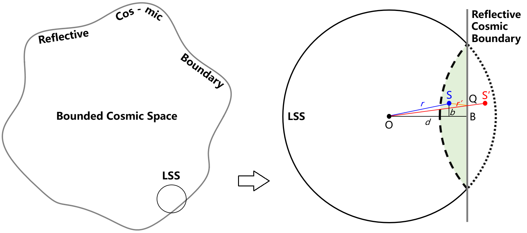
Figure 1: (Left) A possible relation between LSS and BCS. (Right) A zoom-in on the LSS. All objects in the figures are assumed to have fixed comoving coordinates. S is an astrophysical source and S’ is its image in the CB. The path S’O intersects the CB at the point Q. OB is normal to the CB. $r$, $r^{\prime}$ and $d$ are the comoving radial coordinates of S, S’ and B, respectively. $b$ is the distance of S (and S’) to the line OB.

How does the CB evolve as the universe expands? This will depend on the detailed properties of the hidden fluid and the dry vacuum. Here we focus on one particular possibility:

• Firstly, since the properties of gravity and spacetime are determined by the properties of the hidden fluid, variations in the properties of the hidden fluid could be fully responsible for the observed expansion of the universe (see Mei (2022, 2023) for an explicit example).

• Secondly, from the perspective of the dry vacuum, it is possible that the size and shape of the volume occupied by the hidden fluid are fixed.

In the fish tank analogy, the above correspond to saying that the expansion of the universe observed by the “fish” is totally caused by the change of the properties of “water”, while the size and shape of the “fish tank” stay fixed. Motivated by this picture, we will assume that the CB has fixed comoving coordinates, which do not change despite the expansion of the universe.

For the calculations of this paper, we will assume that the interior of the BCS is described by the flat Friedmann-Lemaître-Robertson-Walker (FLRW) metric, $ds^{2}=-dt^{2}+a(t)^{2}(dr^{2}+r^{2}d\Omega_{2})\,$, for which the origin of the spatial coordinates is located at the observer O. The point B in Fig. 1 is placed on the $\hat{x}$-axis, with the comoving Cartesian coordinates: $x_{B}=d\,$, $y_{B}=z_{B}=0$. The source S is located at: $x_{S}=\sqrt{r^{2}-b^{2}}\,$, $y_{S}=b\,$, $z_{S}=0\,$. The comoving distance and luminosity distance of an object at redshift $z$ are determined through $D_{z}=\int_{0}^{z}\frac{dz^{\prime}}{H(z^{\prime})}$ and $D_{L}(z)=(1+z)D_{z}$, respectively, where the Hubble parameter is

$$H(z)=H_{0}\Big{[}\Omega_{\Lambda}+\Omega_{M}(1+z)^{3}+(\Omega_{\gamma}+\Omega_{\nu})(1+z)^{4}\Big{]}^{1/2}\,.$$ (1)

The cosmological parameters are Lahav and Liddle (2024): $H_{0}=100h$ km/s/Mpc with $h\approx 0.677$, $\Omega_{\Lambda}\approx 0.689$, $\Omega_{m}\approx 0.311$, $\Omega_{\gamma}\approx 2.47\times 10^{-5}h^{-2}$, and $\Omega_{\nu}\approx(\sum m_{\nu})(93.12~{}{\rm eV})^{-1}h^{-2}$. There is uncertainty in the neutrino masses, but which are most relevant only in the radiation dominant era. We assume $\sum m_{\nu}=0.1$ eV in this paper Aghanim et al. (2020).

III Detection scheme

Searching for a reflective CB at the high redshift is not easy. Firstly, such surface will have little detectable effect on the CMB due to the homogeneity assumption about the universe, which indicates that the temperature variation along the dashed curve in Fig. 1 is statistically indistinguishable from that along the dotted curve had it not been cutoff by the CB. The sign of the CMB polarization Hu and White (1997) can be flipped by the reflective CB. But this also appears difficult to observe. Secondly, one also cannot rely on parity related characters of individual astrophysical objects to tell if there is a reflective surface, because no universally parity violating character is known for astrophysical objects. So to tell if there is a reflective surface, one must find a way to compare a source to its image caused by the CB.

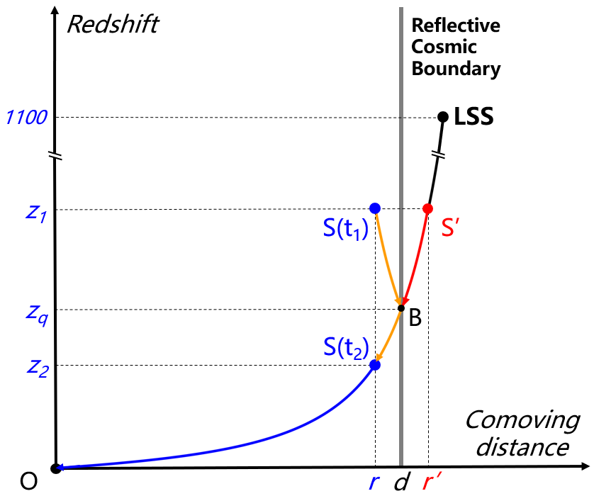
Figure 2: The scheme to detect the CB. The figure has been drawn with $b=0$ for illustration purpose.

A possible detection scheme is illustrated in Fig. 2, in which the past light cone of the observer along the spatial direction O$\rightarrow$B (corresponding to $b=0$ in Fig. 1) is shown. All events/images that can be detected by the observer must lay on the light cone, which is represented by the curve LSS $\rightarrow$ S’ $\rightarrow$ B $\rightarrow$ S($t_{2}$) $\rightarrow$ O in the figure. The physical processes involved in the detection scheme are the following:

• The source S emits a signal at the time $t_{1}$, corresponding to the event S($t_{1}$);

• The signal from S($t_{1}$) firstly travels towards the CB, gets reflected, and then travels toward the observer. For the observer, this is equivalent to having a signal coming from the image S’;

• The source S emits a second signal at $t_{2}$, corresponding to the event S($t_{2}$);

• The signals from S($t_{1}$) and S($t_{2}$) travel toward the observer concurrently, and both are eventually detected by a detector at the location of the observer.

For later convenience, we will refer to S($t_{1}$) as the first source event, S($t_{2}$) the second source event, S’ the image event, S($t_{1}$) and S($t_{2}$) the source events, and S’ and S($t_{2}$) the coincident events.

In this detection scheme, the distance of the CB that can be explored is bounded by the largest possible distance of the image event. Such bound can either come from the technology capability of the detectors or from the availability of suitable sources. If the CB is close enough, one may use an electromagnetic telescope to search for it. In this case, the source events can be two snapshots of a same galaxy. Currently, the most distant galaxy known is JADES-GS-z14-0, which has been detected by JWST at the redshift $z\approx 14.3$ Carniani et al. (2024). This represents the highest redshift (for individual astrophysical objects) that one can explore with a current electromagnetic telescope.

For higher redshifts, one can use GWs. In this case, the source events can be two merger events from the growth history of a MBH. MBHs can start from the remnants of Pop III stars, stellar-mass black holes, massive seeds resulted from very massive stars, primordial black holes, and so on, and grow their masses through accretion and mergers Seoane et al. (2023). Among all the possible MBH seeds, PBHs are particularly interesting because they might have been produced during the inflation Ivanov et al. (1994); Garcia-Bellido et al. (1996); Ivanov (1998). If they can be used to detect the CB, then one can reach redshifts higher than the formation of the first stars and galaxies. Unfortunately, it has been shown that the chance for a PBH to have second-generation merger is very low De Luca et al. (2020). So we will focus on MBHs of non-PBH origin in this paper. This will limit the redshift range of the CB that can be explored. For example, if we fix the redshift of S’ to be at $z=20$, then we can only explore the CB with a redshift no higher than $z=20$.

Below we study what GW sources can be used to detect the CB and what will be needed to confirm the existence of the CB. For all the calculations, unless otherwise specified, we will use the IMRPhenomXHM waveform García-Quirós et al. (2020), and focus on black hole binaries with the major mass (source frame) $m_{1}=1\times 10^{5}{\rm~{}M_{\odot}}$, mass ratio $q=m_{1}/m_{2}=1.2$, source inclination angle $\iota=0.9$ rad, dimensionless spins $s_{1}=0.4$ and $s_{2}=0.2$ (both are assumed to be aligned with the orbital angular momentum), and will assume an observation time $T_{\rm obs}=$ 1 month.

III.1 GW detectors and required source parameters

Several space-based GW detectors are being planned for the 2030s Gong et al. (2021). In this work, we use TianQin Luo et al. (2016); Mei et al. (2021) and LISA Amaro-Seoane et al. (2017) as examples.

TianQin will be consisted of three Earth orbiting satellites, forming a nearly normal triangle constellation with each side measuring about $L_{\rm TQ}\approx\sqrt{3}\times 10^{8}$ m. The sensitivity of TianQin is given by Luo et al. (2016); Mei et al. (2021):

$$S_{n}^{\rm TQ}(f)=\frac{10}{3L_{TQ}^{2}}\left[S_{x}^{\rm TQ}+\frac{4S_{a}^{\rm TQ}}{(2\pi f)^{4}}\Big{(}1+\frac{10^{-4}{\rm Hz}}{f}\Big{)}\right]\times\left[1+0.6{\left(\frac{f}{f_{*}^{\rm TQ}}\right)}^{2}\right],$$ (2)

where $(S_{x}^{\rm TQ})^{1/2}=1\times 10^{-12}{\rm m}/{\rm Hz}^{1/2}$ is the one-way displacement measurement noise, $(S_{a}^{\rm TQ})^{1/2}=1\times 10^{-15}$ m/s²/Hz^1/2 is the residual acceleration of a test mass along the sensitive axis, and $f^{\rm TQ}_{*}=1/(2\pi L_{\rm TQ})\approx 0.28$ Hz is the transfer frequency of TianQin.

LISA will be consisted of three spacecraft forming a nearly normal triangle constellation with each side measuring about $L_{\rm LISA}\approx 2.5\times 10^{9}$ m. The center of the LISA constellation is on the same orbit as the Earth and is at a distance of about 50 million kilometers from the Earth. The plane of the LISA constellation is at about 60^∘ with respect to the ecliptic plane. Apart from its annual orbital motion around the Sun, the LISA constellation also has an annual cartwheel motion. The sensitivity of LISA is given by Robson et al. (2019):

$$S_{n}^{\rm LISA}(f) = \frac{10}{3L_{\rm LISA}^{2}}\left\{S_{x}^{\rm LISA}(f)+\frac{S_{a}^{\rm LISA}(f)}{{(2\pi f)}^{4}}\left[1+\cos^{2}\left(\frac{f}{f_{*}^{\rm LISA}}\right)\right]\right\}\left[1+\frac{6}{10}{\left(\frac{f}{f_{*}^{\rm LISA}}\right)}^{2}\right]\,,$$ (3)

where $f_{*}^{\rm LISA}=1/(2\pi L_{\rm LISA})\approx 0.02$ Hz is the transfer frequency of LISA, and

$$S_{x}^{\rm LISA}(f) = S_{x}^{\rm LISA}\left[1+{\left(\frac{2\times 10^{-3}{\rm Hz}}{f}\right)}^{4}\right]\,,$$

$$S_{a}^{\rm LISA}(f) = S_{a}^{\rm LISA}\left[1+{\left(\frac{4\times 10^{-4}{\rm Hz}}{f}\right)}^{2}\right]\times\left[1+{\left(\frac{f}{8\times 10^{-3}{\rm Hz}}\right)}^{4}\right]\,,$$ (4)

where $(S_{x}^{\rm LISA})^{1/2}=1.5\times 10^{-11}$ m/Hz^1/2 and $(S_{a}^{\rm LISA})^{1/2}=3\times 10^{-15}$ m/s²/Hz^1/2.

Both TianQin and LISA have the goal to detect GWs in the frequency range $10^{-4}$ Hz $\sim$ 1 Hz. But LISA has longer arm-length and can potentially cover a wider frequency range, i.e., $2\times 10^{-5}$ Hz $\sim$ 1 Hz Amaro-Seoane et al. (2017). It is known that the detection capability can be significantly improved if the space-based GW detectors can form a network (see, e.g., Ruan et al. (2020); Gong et al. (2021)). This is also true for the TianQin+LISA network. A detailed study of how TianQin+LISA can improve over each individual detectors can be found in Torres-Orjuela et al. (2024).

Fig. 3 illustrates the detection horizon of TianQin, LISA and TianQin+LISA, and the allowed mass range for possible candidate GW sources at different redshifts, assuming the detection threshold SNR $=8$. One can see that both TianQin and LISA can reach $z>15$ for a wide range of source masses.

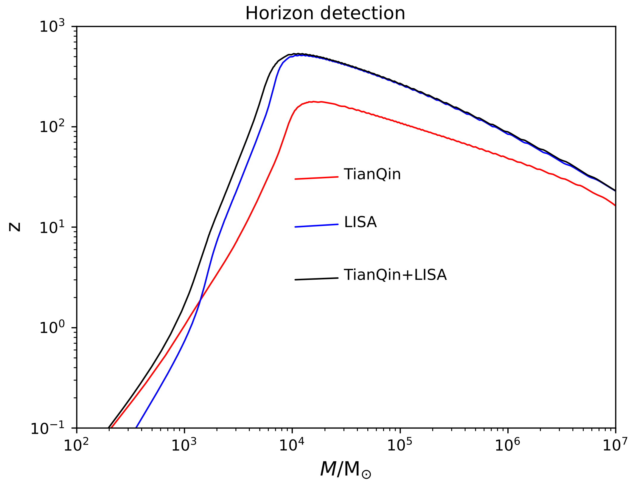
Figure 3: (Left) The detection horizon of TianQin, LISA and TianQin+LISA. (Right) Allowed mass range for candidate GW sources, for S’ at $z=20$ (solid), $S(t_{2})$ at $z_{2}=16.2$, corresponding to $z_{q}=18$ (dashed), and $S(t_{2})$ at $z_{2}=11.6$, corresponding to $z_{q}=15$ (dot-dashed).

III.2 Identifying the coincident events

In order to find the CB, one must firstly detect the coincident GW events. To identify the coincident events, one can check the following:

• Angular separation As indicated in Fig. 1, the angular separation between the coincident events, $\angle$SOS’, must lay within a certain range determined by the distance of the CB, represented by the redshift $z_{q}$ of the point B, and the orientation of the CB, represented by the angle $\angle$S’OB.

• Mass For a pair of coincident GW events, one component of the second source event S($t_{2}$) must be inherited from the remnant black hole of the first source event S($t_{1}$). The remnant black hole of S($t_{1}$) might have experienced some accretion and merger in between S($t_{1}$) and S($t_{2}$). So for a pair of coincident events, S($t_{2}$) must have one component no less massive than the remnant of S($t_{1}$) and equivalently of S’.

• Spin Due to the reflection by the CB, a spin parallel to the CB will have its sign flipped, while that perpendicular to the CB will stay the same. This will lead to a predictable relation between the spin of the remnant of S’ and that of one of the components of S($t_{2}$), given that the location of CB is known and that the spin of the remnant of S($t_{1}$) has not been significantly altered by accretion or merger in between S($t_{1}$) and S($t_{2}$).

Fig. 4 illustrates the dependence of $z_{2}$ and $\angle$SOS’ on $\angle$S’OB and $z_{q}$. In the figure, the image event S’ is fixed at the redshift $z_{1}=20$, and $z_{q}$ is varied from 10 to 20. Correspondingly, $z_{2}$ can vary from about 5 to 20, which also depends on $\angle$S’OB. One can see that for $z_{q}>15$, one always has approximately $\angle$SOS’$<0.5^{\circ}$. Such a small angular separation between the coincident events is helpful in that it can significantly shorten the list of potential candidates.

Once the extrinsic parameters match, one can then look at the intrinsic parameters. Fig. 5 (top left and right) illustrates the expected measurement precision for the mass $M$ and dimensionless spin $s$ of the component of $S(t_{2})$ that is inherited from the remnant black hole of $S(t_{1})$. For a worst case scenario, we focus on $z_{2}\approx z_{q}\approx z_{1}=20$. The remnant black hole will become a component in the merger event of $S(t_{2})$. For these parameters, LISA dominates the contribution to the TianQin+LISA network. One can see that, even for sources located at redshift as high as $z=20$, one still has $\Delta M/M<10\%$ and $\Delta s<0.1$ for a wide range of source masses. The best precisions can reach $\Delta M/M\sim{\cal O}(10^{-5})$ and $\Delta s\sim{\cal O}(10^{-4})$.

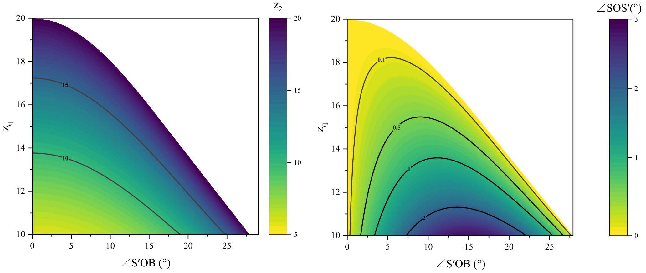
Figure 4: The dependence of $z_{2}$ and $\angle$SOS’ on $\angle$S’OB and $z_{q}$.

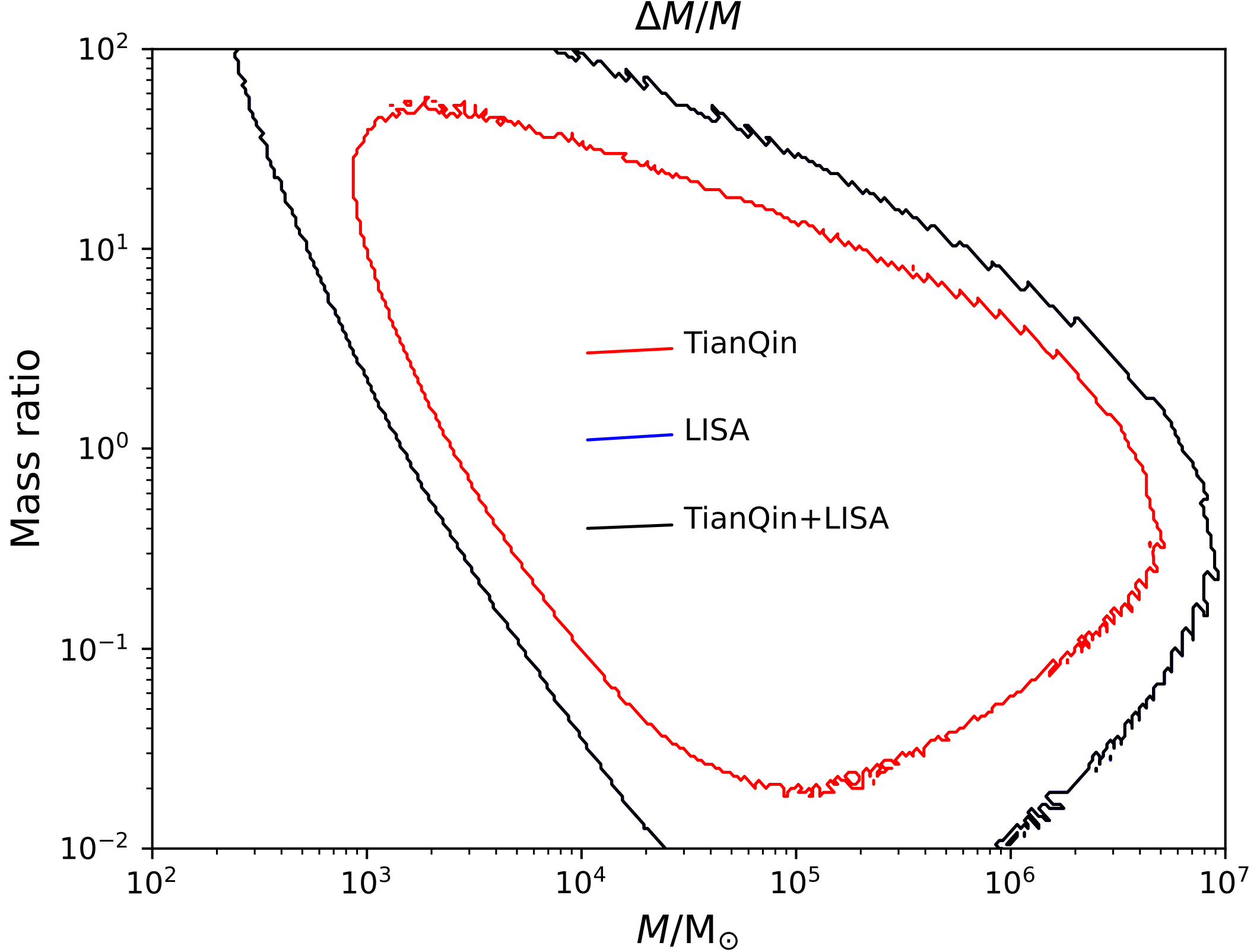
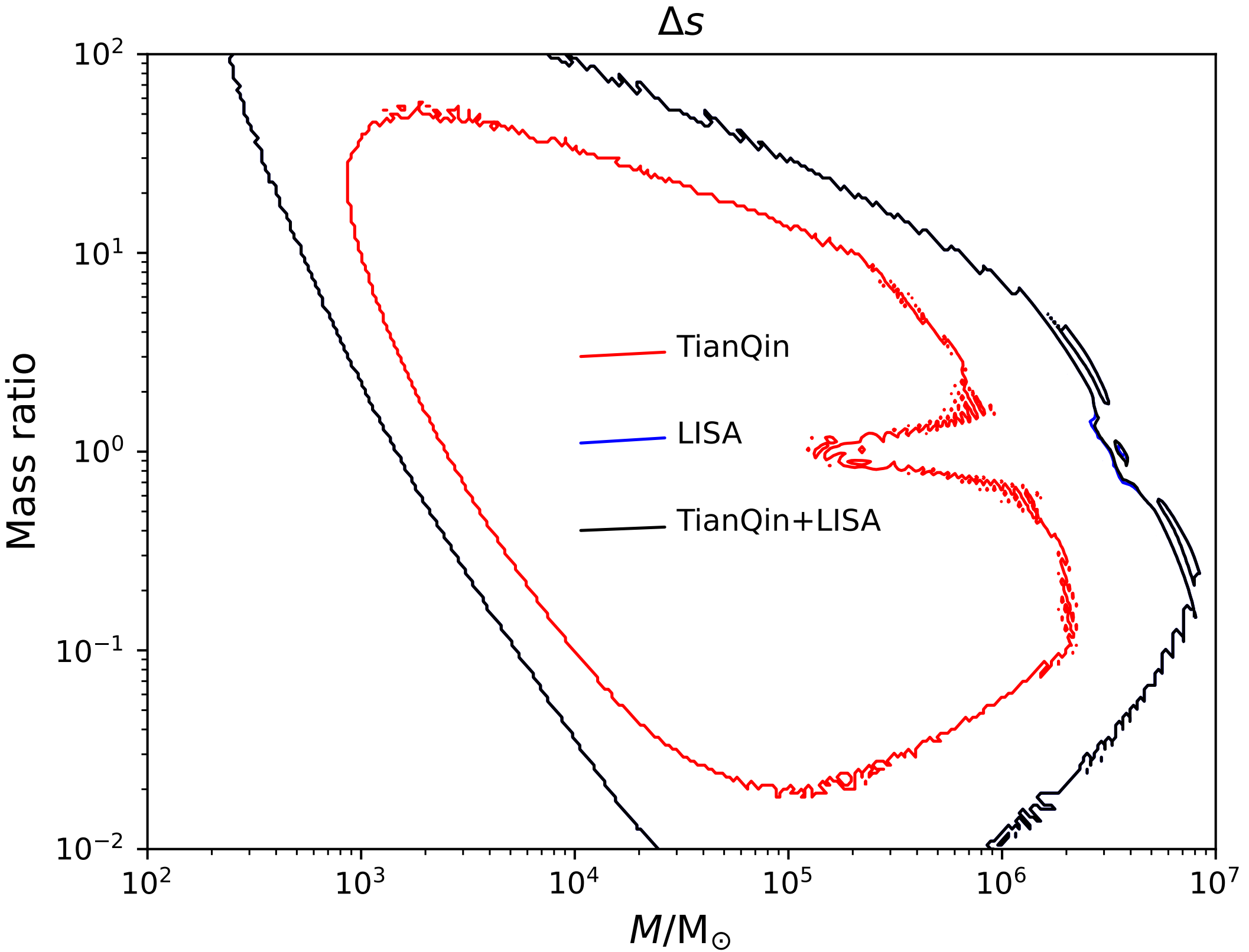
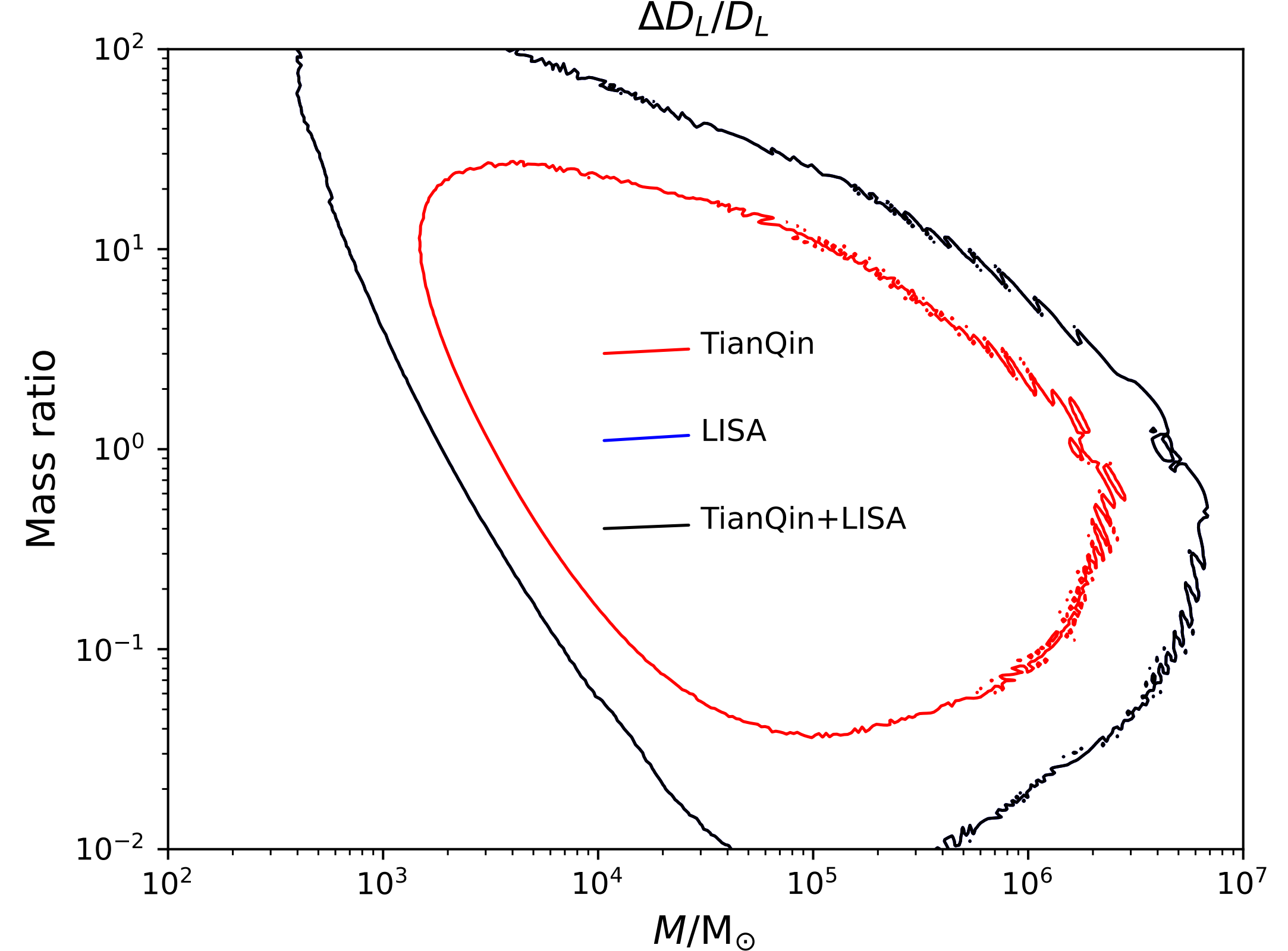
Figure 5: The expected precision for measuring mass, spin and luminosity distance for a source located at $z=20$. Regions inside the contours are for $\Delta M/M<10\%$ (top left), $\Delta s<0.1$ (top right) and $\Delta D_{L}/D_{L}<10\%$ (buttom). Presented in the sequence: (TianQin, LISA, TianQin+LISA), the highest precisions in each plot are: $\Delta M/M=(2.7,1.4,1.2)\times 10^{-5}$, $\Delta s=(2.5,1.2,1.1)\times 10^{-4}$ and $\Delta D_{L}/D_{L}=(12.4,4.3,4.1)\times 10^{-3}$.

III.3 Necessary conditions to confirm the CB

With the present detection scheme, it is difficult to confirm a pair of coincident events to the 100% level, even when all the extrinsic and the intrinsic parameters are as predicted. In order to confirm the presence of the CB to a high confidence level, it is necessary to have multiple pairs of coincident events, with all of which predicting the same location for the CB. This will be challenging not only in terms of the number of events that need to be detected, but also in terms of the precision that one needs to locate the sources.

A reliable assessment of the chance to detect multiple pairs of coincident events is difficult and is beyond the scope of this paper. Here we only want to remark that, given the weight that the possible presence of the CB bears on our entire view of the universe, it is always worthwhile searching for potential signatures of it, no matter how small the chance is.

For the precision to determine the space location of the sources, Fig. 5 (bottom) illustrates the expected precision for measuring the luminosity distance of $S(t_{2})$ at $z_{2}\approx 20$. One can see that the luminosity distance can be determined to better than $\Delta D_{L}/D_{L}=10\%$ for a large range of source masses. The best precisions can reach $\Delta D_{L}/D_{L}\sim{\cal O}(10^{-3})$.

From Fig. 4, one can see that $\angle$SOS’ does not depend on $\angle$S’OB very sensitively. This means that one will need to measure $\angle$SOS’ very precisely to determine the orientation of CB. For example, for $z_{q}>15$, one needs to measure $\angle$SOS’ to better than about $0.5^{\circ}$. Fig. 6 illustrates the expected precision of the angular resolution, $\delta\theta=\sqrt{\Delta\Omega/\pi}$, for a source located at $z=20$. In the plots, the exact shape of the contours significantly depends on the choice of the source parameters, but the contrast between the capability of different detector configurations is roughly the same. One can see that the TianQin+LISA network can significantly increase the region of the sky in which a source can be localized to better than $\delta\theta\sim{\cal O}(0.5^{\circ})$. So a detector network like TianQin+LISA is essential in help increasing the chance to determine the location of the CB, given that enough pairs of coincident events can be detected.

Fig. 6 also shows that for $z_{q}>18$, the angular resolution is always worse than $0.1^{\circ}$ even with the TianQin+LISA network. From Fig. 4, this means that one will not be able to determine the orientation of CB in this case. But the brighter side is, Fig. 4 also indicates that one always has $\angle$S’OB $<10^{\circ}$ for $z_{q}>18$.

Finally, we remark that the above conclusions have been obtained by fixing the source at $z=20$. The quantitative result can become different if it is located at other redshifts.

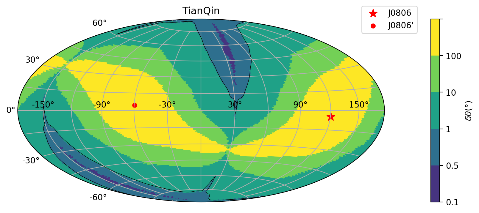
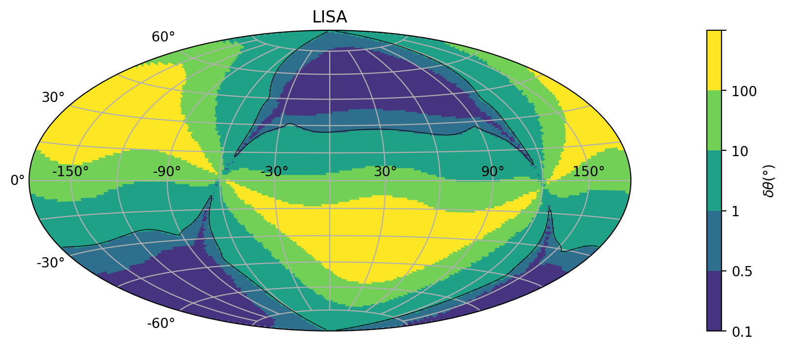
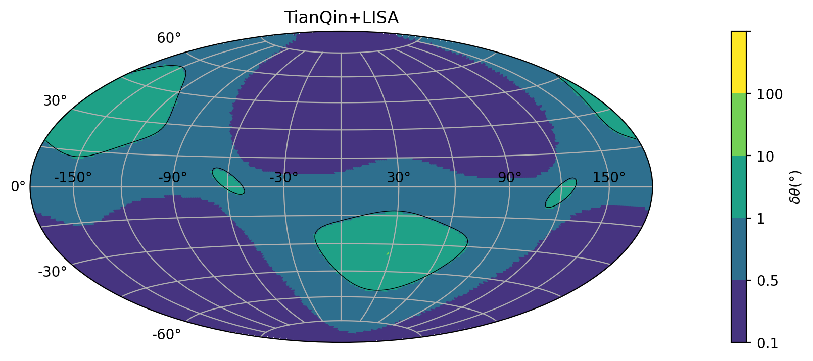
Figure 6: The expected precision of angular resolution for a source at $z=20$ with TianQin, LISA and TianQin+LISA. J0806’ indicates the opposite direction of J0806. The orbital angular momenta of all the sources are fixed at the direction $\theta_{L}=\phi_{L}=0.6$ rad. The exact shape of the contours will change significantly if one modifies the source parameters, but the contrast between the capability of different detectors and detector network is roughly the same.

IV Summary

In this paper, we have studied the potential of using GWs to detect the possible presence of a CB at the high redshift. The CB is assumed to have fixed comoving coordinates, being reflective for both electromagnetic waves and GWs. We focus on MBHs of non-PBH origin and find that, with the future space-based GW detectors like TianQin and LISA, a large variety of MBHs with masses roughly in the range ${\cal O}(10^{3}{\rm~{}M_{\odot}})\sim{\cal O}(10^{6}{\rm~{}M_{\odot}})$ can be used to detect the CB.

To find the CB, we have studied a detection scheme that relies on detecting two merger events from the growth history of a MBH. We find that, for a CB located at the high redshift ($z_{q}>15$), the angular separation between a pair of coincident events is always smaller than about $0.5^{\circ}$. The relative precision of mass and luminosity distance can be determined to better than the 10% level, and the dimensionless spin can be determined to better than the 0.1 level. Combined, these capabilities can provide strong evidence to identify possible pairs of coincident GW events.

In order to confirm the presence of the CB to a high confidence level, however, it is necessary to detect multiple pairs of coincident events. In this case, a detector network like TianQin+LISA is crucial in help improving the chance to precisely determine the orientation of the CB. The chance for detecting a pair of coincident events is presumably low, and the chance to detect multiple pairs of coincident events is even lower. So the possibility to prove or disprove the presence of the cosmic boundary largely depends on how likely one can detect multiple pairs of coincident gravitational wave events. This is a key restriction to the detection scheme described in this paper.

Due to the importance of the possible nontrivial global structure of the cosmic space to our entire view of the universe, however, it is always worthwhile searching for potential signatures of it in the GW data expected in the 2030s, even if the predicted chance is very small.

References

- Aghanim et al. (2020) N. Aghanim et al. (Planck), Astron. Astrophys. 641, A6 (2020), [Erratum: Astron.Astrophys. 652, C4 (2021)], arXiv:1807.06209 [astro-ph.CO] .
- Lahav and Liddle (2024) O. Lahav and A. R. Liddle, (2024), arXiv:2403.15526 [astro-ph.CO] .
- Eskilt et al. (2024) J. R. Eskilt et al. (COMPACT), JCAP 03, 036 (2024), arXiv:2306.17112 [astro-ph.CO] .
- Lachieze-Rey and Luminet (1995) M. Lachieze-Rey and J.-P. Luminet, Phys. Rept. 254, 135 (1995), arXiv:gr-qc/9605010 .
- Levin (2002) J. J. Levin, Phys. Rept. 365, 251 (2002), arXiv:gr-qc/0108043 .
- Cornish et al. (1998) N. J. Cornish, D. N. Spergel, and G. D. Starkman, Class. Quant. Grav. 15, 2657 (1998), arXiv:astro-ph/9801212 .
- de Oliveira-Costa et al. (2004) A. de Oliveira-Costa, M. Tegmark, M. Zaldarriaga, and A. Hamilton, Phys. Rev. D 69, 063516 (2004), arXiv:astro-ph/0307282 .
- Cornish et al. (2004) N. J. Cornish, D. N. Spergel, G. D. Starkman, and E. Komatsu, Phys. Rev. Lett. 92, 201302 (2004), arXiv:astro-ph/0310233 .
- Shapiro Key et al. (2007) J. Shapiro Key, N. J. Cornish, D. N. Spergel, and G. D. Starkman, Phys. Rev. D 75, 084034 (2007), arXiv:astro-ph/0604616 .
- Mota et al. (2010) B. Mota, M. J. Reboucas, and R. Tavakol, Phys. Rev. D 81, 103516 (2010), arXiv:1002.0834 [astro-ph.CO] .
- Bielewicz and Banday (2011) P. Bielewicz and A. J. Banday, Mon. Not. Roy. Astron. Soc. 412, 2104 (2011), arXiv:1012.3549 [astro-ph.CO] .
- Bielewicz et al. (2012) P. Bielewicz, A. J. Banday, and K. M. Gorski, Mon. Not. Roy. Astron. Soc. 421, 1064 (2012), arXiv:1111.6046 [astro-ph.CO] .
- Vaudrevange et al. (2012) P. M. Vaudrevange, G. D. Starkman, N. J. Cornish, and D. N. Spergel, Phys. Rev. D 86, 083526 (2012), arXiv:1206.2939 [astro-ph.CO] .
- Aurich and Lustig (2013) R. Aurich and S. Lustig, Mon. Not. Roy. Astron. Soc. 433, 2517 (2013), arXiv:1303.4226 [astro-ph.CO] .
- Ade et al. (2014) P. A. R. Ade et al. (Planck), Astron. Astrophys. 571, A26 (2014), arXiv:1303.5086 [astro-ph.CO] .
- Ade et al. (2016) P. A. R. Ade et al. (Planck), Astron. Astrophys. 594, A18 (2016), arXiv:1502.01593 [astro-ph.CO] .
- Mihaylov et al. (2023) D. P. Mihaylov et al. (COMPACT), JCAP 01, 030 (2023), [Erratum: JCAP 04, E01 (2024)], arXiv:2211.02603 [astro-ph.CO] .
- Akrami et al. (2024) Y. Akrami et al. (COMPACT), Phys. Rev. Lett. 132, 171501 (2024), arXiv:2210.11426 [astro-ph.CO] .
- zhi Fang and Sato (1983) L. zhi Fang and H. Sato, Communications in Theoretical Physics 2, 1055 (1983).
- Fagundes and Wichoski (1987) H. V. Fagundes and U. F. Wichoski, the Astrophysical Journal Letters 322, L5 (1987).
- Roukema (1996) B. F. Roukema, Mon. Not. Roy. Astron. Soc. 283, 1147 (1996), arXiv:astro-ph/9603052 .
- Lehoucq et al. (1996) R. Lehoucq, M. Lachieze-Rey, and J. P. Luminet, Astron. Astrophys. 313, 339 (1996), arXiv:gr-qc/9604050 .
- Luminet and Roukema (1999) J.-P. Luminet and B. F. Roukema, in NATO Advanced Study Institute: Summer School on Theoretical and Observational Cosmology (1999) arXiv:astro-ph/9901364 .
- Fujii and Yoshii (2011) H. Fujii and Y. Yoshii, Astron. Astrophys. 529, A121 (2011), arXiv:1103.1466 [astro-ph.CO] .
- Fujii and Yoshii (2013) H. Fujii and Y. Yoshii, Astrophys. J. 773, 152 (2013), arXiv:1306.2737 [astro-ph.CO] .
- Roukema et al. (2014) B. F. Roukema, M. J. France, T. A. Kazimierczak, and T. Buchert, Mon. Not. Roy. Astron. Soc. 437, 1096 (2014), arXiv:1302.4425 [astro-ph.CO] .
- Luminet (2016) J.-P. Luminet, Universe 2, 1 (2016), arXiv:1601.03884 [astro-ph.CO] .
- Weatherley et al. (2003) S. J. Weatherley, S. J. Warren, S. M. Croom, R. J. Smith, B. J. Boyle, T. Shanks, L. Miller, and M. P. Baltovic, Monthly Notices of the Royal Astronomical Society 342, L9 (2003), arXiv:astro-ph/0304290 [astro-ph] .
- Carniani et al. (2024) S. Carniani, K. Hainline, F. D’Eugenio, D. J. Eisenstein, P. Jakobsen, J. Witstok, B. D. Johnson, J. Chevallard, R. Maiolino, J. M. Helton, C. Willott, B. Robertson, S. Alberts, S. Arribas, W. M. Baker, R. Bhatawdekar, K. Boyett, A. J. Bunker, A. J. Cameron, P. A. Cargile, S. Charlot, M. Curti, E. Curtis-Lake, E. Egami, G. Giardino, K. Isaak, Z. Ji, G. C. Jones, M. V. Maseda, E. Parlanti, T. Rawle, G. Rieke, M. Rieke, B. Rodríguez Del Pino, A. Saxena, J. Scholtz, R. Smit, F. Sun, S. Tacchella, H. Übler, G. Venturi, C. C. Williams, and C. N. A. Willmer, arXiv e-prints , arXiv:2405.18485 (2024), arXiv:2405.18485 [astro-ph.GA] .
- Seoane et al. (2013) P. A. Seoane et al. (eLISA), (2013), arXiv:1305.5720 [astro-ph.CO] .
- Amaro-Seoane et al. (2017) P. Amaro-Seoane et al. (LISA), (2017), arXiv:1702.00786 [astro-ph.IM] .
- Luo et al. (2016) J. Luo et al. (TianQin), Class. Quant. Grav. 33, 035010 (2016), arXiv:1512.02076 [astro-ph.IM] .
- Hu et al. (2017) Y.-M. Hu, J. Mei, and J. Luo, Natl. Sci. Rev. 4, 683 (2017).
- Wang et al. (2019) H.-T. Wang et al., Phys. Rev. D 100, 043003 (2019), arXiv:1902.04423 [astro-ph.HE] .
- Mei et al. (2021) J. Mei et al. (TianQin), PTEP 2021, 05A107 (2021), arXiv:2008.10332 [gr-qc] .
- Torres-Orjuela et al. (2024) A. Torres-Orjuela, S.-J. Huang, Z.-C. Liang, S. Liu, H.-T. Wang, C.-Q. Ye, Y.-M. Hu, and J. Mei, Sci. China Phys. Mech. Astron. 67, 259511 (2024), arXiv:2307.16628 [gr-qc] .
- Hu and Wu (2017) W.-R. Hu and Y.-L. Wu, Natl. Sci. Rev. 4, 685 (2017).
- Evans et al. (2021) M. Evans et al., (2021), arXiv:2109.09882 [astro-ph.IM] .
- Maggiore et al. (2020) M. Maggiore et al., JCAP 03, 050 (2020), arXiv:1912.02622 [astro-ph.CO] .
- Bailes et al. (2021) M. Bailes et al., Nature Rev. Phys. 3, 344 (2021).
- Branchesi et al. (2023) M. Branchesi et al., JCAP 07, 068 (2023), arXiv:2303.15923 [gr-qc] .
- Seoane et al. (2023) P. A. Seoane et al. (LISA), Living Rev. Rel. 26, 2 (2023), arXiv:2203.06016 [gr-qc] .
- Dayal et al. (2019) P. Dayal, E. M. Rossi, B. Shiralilou, O. Piana, T. R. Choudhury, and M. Volonteri, Mon. Not. Roy. Astron. Soc. 486, 2336 (2019), arXiv:1810.11033 [astro-ph.GA] .
- Pacucci and Loeb (2020) F. Pacucci and A. Loeb, Astrophys. J. 895, 95 (2020), arXiv:2004.07246 [astro-ph.GA] .
- Piana et al. (2020) O. Piana, P. Dayal, M. Volonteri, and T. R. Choudhury, Mon. Not. Roy. Astron. Soc. 500, 2146 (2020), arXiv:2009.13505 [astro-ph.GA] .
- Liu and Inayoshi (2024) H. Liu and K. Inayoshi, (2024), arXiv:2409.18194 [astro-ph.CO] .
- Hu (2009) B. L. Hu, J. Phys. Conf. Ser. 174, 012015 (2009), arXiv:0903.0878 [gr-qc] .
- Sindoni (2012) L. Sindoni, SIGMA 8, 027 (2012), arXiv:1110.0686 [gr-qc] .
- Carlip (2014) S. Carlip, Stud. Hist. Phil. Sci. B 46, 200 (2014), arXiv:1207.2504 [gr-qc] .
- Linnemann and Visser (2018) N. S. Linnemann and M. R. Visser, Stud. Hist. Phil. Sci. B 64, 1 (2018), arXiv:1711.10503 [physics.hist-ph] .
- Bhattacharyya et al. (2008) S. Bhattacharyya, V. E. Hubeny, S. Minwalla, and M. Rangamani, JHEP 02, 045 (2008), arXiv:0712.2456 [hep-th] .
- Rangamani (2009) M. Rangamani, Class. Quant. Grav. 26, 224003 (2009), arXiv:0905.4352 [hep-th] .
- Hubeny et al. (2012) V. E. Hubeny, S. Minwalla, and M. Rangamani, in Theoretical Advanced Study Institute in Elementary Particle Physics: String theory and its Applications: From meV to the Planck Scale (2012) pp. 348–383, arXiv:1107.5780 [hep-th] .
- Maldacena (1998) J. M. Maldacena, Adv. Theor. Math. Phys. 2, 231 (1998), arXiv:hep-th/9711200 .
- Mei (2022) J. Mei, Eur. Phys. J. Plus 137, 578 (2022).
- Mei (2023) J. Mei, Eur. Phys. J. C 83, 16 (2023), arXiv:2210.05434 [gr-qc] .
- Hu and White (1997) W. Hu and M. J. White, New Astron. 2, 323 (1997), arXiv:astro-ph/9706147 .
- Ivanov et al. (1994) P. Ivanov, P. Naselsky, and I. Novikov, Phys. Rev. D 50, 7173 (1994).
- Garcia-Bellido et al. (1996) J. Garcia-Bellido, A. D. Linde, and D. Wands, Phys. Rev. D 54, 6040 (1996), arXiv:astro-ph/9605094 .
- Ivanov (1998) P. Ivanov, Phys. Rev. D 57, 7145 (1998), arXiv:astro-ph/9708224 .
- De Luca et al. (2020) V. De Luca, G. Franciolini, P. Pani, and A. Riotto, JCAP 04, 052 (2020), arXiv:2003.02778 [astro-ph.CO] .
- García-Quirós et al. (2020) C. García-Quirós, M. Colleoni, S. Husa, H. Estellés, G. Pratten, A. Ramos-Buades, M. Mateu-Lucena, and R. Jaume, Phys. Rev. D 102, 064002 (2020), arXiv:2001.10914 [gr-qc] .
- Gong et al. (2021) Y. Gong, J. Luo, and B. Wang, Nature Astron. 5, 881 (2021), arXiv:2109.07442 [astro-ph.IM] .
- Robson et al. (2019) T. Robson, N. J. Cornish, and C. Liu, Class. Quant. Grav. 36, 105011 (2019), arXiv:1803.01944 [astro-ph.HE] .
- Ruan et al. (2020) W.-H. Ruan, C. Liu, Z.-K. Guo, Y.-L. Wu, and R.-G. Cai, Nature Astron. 4, 108 (2020), arXiv:2002.03603 [gr-qc] .