Misty, patchy, and turbulent: constraining the cold circumgalactic medium with mCC

Abstract

The circumgalactic medium (CGM) is the largest baryon reservoir around galaxies, but its extent, mass, and temperature distribution remain uncertain. We propose that cold gas in the CGM resides primarily in $\sim 100\hbox{--}10^{4}$ cloud complexes (CCs), each containing a mist of tiny cold cloudlets dispersed in a warm/hot medium ($\sim 10^{5}\hbox{--}10^{6}$ K). Modeling CCs as uniform and misty simplifies the calculation of observables like ion absorption columns compared to resolving tiny individual cloudlets. Using Monte Carlo simulations, we explore how CC properties affect the observed spread in column densities. A power-law distribution of CCs ($dN_{\rm CC}/dR\propto R^{-1.2}$) reproduces MgII equivalent width (EW) and column density distribution trends with impact parameter ($R_{\perp}$). We show that the area-averaged MgII column density, combined with the covering fraction of CCs, provides a robust proxy for estimating the cold CGM mass, independent of other model parameters. Modeling individual CCs demonstrates that turbulent broadening blends cloudlet absorption lines, allowing CCs to approximate the observational effects of their constituent cloudlets analytically. Direct simulations of cloudlets within multiple CCs confirm the computational challenges of fully resolving the mist-like structure. Comparing modeled MgII absorption with observations, we estimate the cold CGM mass of Milky Way-like galaxies to be $\sim 10^{10}\,M_{\odot}$, about $10\%$ of the total CGM mass. This work provides a practical framework for connecting CGM models with observations, shedding light on the cold gas distribution in galaxy halos and its role in the galactic baryon cycle.

1 Introduction

Circumgalactic medium (CGM) is the vast reservoir of gas surrounding the stellar disk and the Interstellar medium (ISM) of galaxies (Tumlinson et al., 2017; Faucher-Giguère & Oh, 2023). Various observations and numerical simulations suggest CGM to be multiphase with gas temperature in the range $\sim 10^{4}$-$10^{7}$ K. Unlike the intracluster medium (ICM) of massive clusters of galaxies, which has been mapped in X-ray emission (a recent review is Donahue & Voit 2022), the hot CGM in Milky Way-like galaxies (like X-ray emitting ICM, also likely to be the mass/volume dominant phase) is too dilute and compact to be mapped in emission. The cold/warm gas ($\sim 10^{4-5}$ K) in the CGM of foreground external galaxies is detected in absorption lines of low/intermediate ionization metal ions like MgII, SiII, CII, CIV, OVI in the spectra of bright background sources (typically quasars; Srianand & Khare 1993; Tumlinson et al. 2011; Nielsen et al. 2013; Werk et al. 2013; Nielsen et al. 2016; Dutta et al. 2020; Huang et al. 2021; Qu et al. 2023; Wu et al. 2024; Chen et al. 2024). More recently, cold gas has also been observed in MgII emission (Burchett et al. 2021; Nelson et al. 2021; Pessa et al. 2024), but it is sensitive to the densest cold gas.

A fundamental but unconstrained physical property of the CGM (unless qualified, we refer to the CGM of Milky Way-like galaxies) is its mass fraction in the cold phase. Although the cold ion (e.g., Mg II) column density (inferred from absorption lines) directly counts the number of ions along the sightline, the cold CGM mass is highly uncertain because of a large variation in the inferred column density at the same distance from the center (c.f. Figure 3). A key result of this paper is that the combination of the average column density and the area covering fraction (both observationally available quantities) provides a robust estimate of the cold gas mass in the CGM ($\sim 10^{10}M_{\odot}$ for Milky Way-like galaxies). Metal ion absorption is also affected by the elemental abundances, the photoionizing background, and non-equilibrium effects. Since the dispersion measure provides column density of free electrons, which is not affected by these complications, fast radio bursts (FRBs) are promising probes of the total CGM mass (Prochaska & Zheng 2019; Cook et al. 2023). However, we cannot distinguish the various thermal phases of the CGM from FRB dispersion measures.

The cold gas in the CGM likely has various formation channels (Decataldo et al. 2024), including, e.g, cooling from hot gas in the CGM due to thermal instability (McCourt et al. 2012; Voit et al. 2017), cosmological accretion into galaxy (Afruni et al. 2019), stellar and AGN outflows (Augustin et al. 2021; Burchett et al. 2021), and stripping from satellite galaxies (Rubin et al. 2012; Roy et al. 2024). The models presented in this paper are agnostic to the specific cold gas formation mechanisms but provide a tool for building phenomenological models of the mass and radial distribution of the cold gas in the CGM. This cold gas is observed to have an area covering fraction of the order of unity (Dutta et al. 2020; Huang et al. 2021), while the volume fraction is expected to be $\lesssim 1\%$ (Faerman & Werk 2023; Dutta et al. 2024). This suggests that the cold gas is not uniformly distributed in the CGM unlike the hot gas ($\sim 10^{6}$ K) but is rather distributed in clumpy and misty structures dispersed in the hot CGM.

Recently, Dutta et al. (2024) (hereafter D24) modeled the cold gas with a three-phase, one-zone CGM model. One zone model refers to filling all the cold gas uniformly as a mist in the entire CGM. We refer to this as the mCGM (misty CGM) model. They modeled the cold gas in one of the TNG-50 halos (Nelson et al. 2020) and predicted the baseline column density of MgII to be $\sim 10^{13}\,\rm cm^{-2}$ (the solid cyan line in their Fig. 11). This is smaller than the typical observed column density, despite the large scatter in observed values and several stringent upper limits. This suggests that the cold gas does not block all sightlines. For mCGM model, the cold gas is distributed in the entire CGM volume, which would result in a low number density and therefore a low column density. To explain the empty sightlines and the observed large scatter in the column density, the cold gas ought to be distributed in a smaller volume than the entire CGM. This will result in higher particle number density and, therefore, a larger column density for sightlines passing through cold clouds and non-detection along the empty sightlines. One can distribute the cold gas in multiple $\sim 10$ kpc cloud complexes (CCs) rather than uniformly throughout the entire CGM and better match the observations. In this paper, we extend the work of D24, moving beyond a completely misty CGM to a more realistic CGM filled with misty cloud complexes. We refer to our model based on CCs as mCC model, which stands for misty cloud complex.

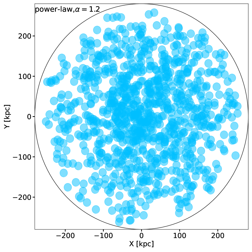
Figure 1: LOS projected distribution (power-law distribution) of $10^{3}$ CCs each of radius $10$ kpc in the CGM of radius $280$ kpc with a power-law index $\alpha=1.2$. Notice that there are numerous empty regions towards the outer regions of CGM, as well as comparatively fewer empty regions in the central region. The LOSs passing through these regions will not produce absorption. Meanwhile, the LOSs passing through the regions with multiple CC (mostly in the central regions) will result in a high column density of the ions. Thus, the misty CC model explains the large scatter in the observed column densities of the ions tracing the cold gas.

Motivated by observations and simulations (area covering fraction and volume fraction), we assume that the cold gas resides in a few thousand cloudy structures. We refer to these structures as ‘cloud complexes’ (CCs) following Hummels et al. (2023) (hereafter H23). These CCs are filled with tiny cold gas cloudlets. For illustration, in Figure 1, we show the line of sight (LOS) projected distribution of CCs in the CGM where the number density of CCs as a function of distance from the center follows a power-law profile with a power-law index of $1.2$. There are $10^{3}$ CCs in total, each of radius $10$ kpc distributed in the CGM of radius $280$ kpc. The estimated area covering fraction of CCs is $\sim 1.3$ assuming no overlap of CCs in the LOS projected plane. Shooting $10^{4}$ lines of sight through the CGM results in $\approx 10^{3}$ empty sightlines. Therefore, the true covering fraction is $\approx 0.9$, which suggests that there are some empty sightlines without any CCs (as can be seen in Figure 1). The LOSs passing through these regions will result in no detection of cold gas (corresponding to the upper limits on the MgII column in Figure 3). These empty regions are everywhere in the CGM (fewer in the central region than in the outskirts). The LOSs passing through multiple CCs will result in a higher column density of cold ions. Therefore, a large scatter in the column density values at approximately the same impact parameter is a natural outcome of the distribution of cold gas in CCs rather than its uniform distribution in the entire CGM (c.f. Figure 4).

In this work, we study and analyze the distribution of CCs in the CGM and the distribution of cloudlets within these CCs. A Monte Carlo distribution of cloudlets within CCs was also studied by H23. They generated cloudlets in a CC, and based on their analytic halo scale model for cold mass distribution, they predicted the equivalent width (EW) distribution of the MgII line. The CCs in the CGM are analogous to terrestrial clouds that are made up of an astronomical number of tiny water droplets. Similarly, the CGM observations of individual absorption components at high-velocity resolution suggest the cloudlets to be $\lesssim 1$ pc (e.g., Fig. 17 of Sameer et al. 2024 and Fig. 3 of Chen et al. 2023). It is impossible to computationally model such an enormous number of cloudlets within a CC from first principles. Instead, we take a complementary and computationally tractable approach, treat the cloudlets within a CC in the mist limit, and generate Monte Carlo realizations of a manageable number of CCs. Our misty CCs have a turbulent velocity spread which follows the Kolmogorov scaling of velocity fluctuations as a function of the CC size ($\sigma_{\rm turb,CC}\propto R_{\rm CC}^{1/3}$).

Beyond the mCC model, we create Monte Carlo realizations of cloudlets in a single CC with an increasing number of smaller cloudlets to show that the misty CC approximation provides a satisfactory description of the otherwise computationally expensive realization of an enormous number of cloudlets within a CC (the approach followed by H23; see section 3). Later, we generate Monte Carlo realizations of not only individual cloudlets within a single CC but also the distribution of CCs across the CGM (section 4). In this computationally prohibitive model, we cannot reach the misty limit, but we compare the distribution of EWs and constrain the model parameters. Thus, our mCC model acts as a tractable bridge between the simple misty CGM model of D24 and the computationally expensive Monte Carlo distribution of cloudlets within CCs (H23).

The MgII doublet metal transition $\lambda\lambda\,2796,2803$ is well observed and studied in the absorption of quasar light from the intervening CGM of external galaxies. In this work, we focus on MgII $\lambda 2796$, but our model can also be used to analyze other cold ions like SiII, and CII, and with simple extension also intermediate ions such as CIV and OVI. (c.f. section 5.3).

Section 2 introduces our analytical framework with the distribution of misty CCs in the CGM. In Section 3, we focus on the distribution of cloudlets within a single CC and quantify the mist limit in the velocity space. In section 4 we work with a Monte Carlo distribution of cloudlets within CCs (rather than the misty limit) distributed throughout the CGM, followed by discussion and summary in sections 5 and 6, respectively.

2 Misty cloud complexes in the CGM

One of the caveats of the misty CGM model of D24 is that it predicts cold gas along all LOSs, which is inconsistent with observations (see numerous upper limits in Figure 3). If instead, the cold gas is spread non-uniformly in smaller CCs, there will be sightlines not covered by cold gas (see Figure 1). In this section, we model the cold gas with multiple misty CCs by extending the misty CGM model of D24. We distribute these CCs in the CGM and compute the observables (column density, equivalent width distributions, covering fraction) to be compared with observations. For concreteness, we compare a uniform and a power-law distribution of CCs in the CGM. We consider the CCs to be misty, with the area coverage fraction of cloudlets within a CC equal to unity ($f_{A}^{\rm cl}=1$). The area covering fraction of CCs ($f_{A}^{\rm CC}$) is the fraction of the CGM area occupied by CCs. This cannot exceed unity if we do not separately count the areas of overlapping CCs; otherwise, it may exceed unity. We mostly use $f_{A}^{\rm CC}$ in the former sense.

If $M_{\rm cold}$ and $N_{\rm CC}$ are the total cold gas mass and the total number of CCs in the CGM, respectively, then the mass of each CC is $M_{\rm CC}=M_{\rm cold}/N_{\rm CC}$, assuming (for simplicity) that all the CCs have the same mass. The average number density of cold gas in each CC (distinct from the physical density of the cold gas) is then $\langle n_{\rm gas}\rangle=3M_{\rm CC}/(4\ \pi R_{\rm CC}^{3}\ \mu m_{\rm p})$, where $R_{\rm CC}$ is the radius of CC and $\mu$ is the mean molecular weight which we assume to be $0.6$.

2.1 The mist limit

Before exploring the distribution of misty CCs across the CGM, it is important to recapitulate what is meant by the ‘mist limit’ within a CC. Here we extend the discussion in section 4.2 of D24, which uses Cartesian cloudlets (geometry only introduces order unity factors without altering the scaling relations with the parameters) of uniform size. The parameters for such a CC are the volume filling fraction $f_{V}$, number of cloudlets $N_{\rm cl}$, and the CC size $L$. The column density of the cold gas in the misty limit is given by $nLf_{V}$, where $n$ is the physical number density of the cold gas. The area covering fraction is unity provided the average number of cloudlets along a sightline $f_{V}^{2/3}N_{\rm cl}^{1/3}$ exceeds unity, that is when $N_{\rm cl}\gtrsim f_{V}^{-2}$.

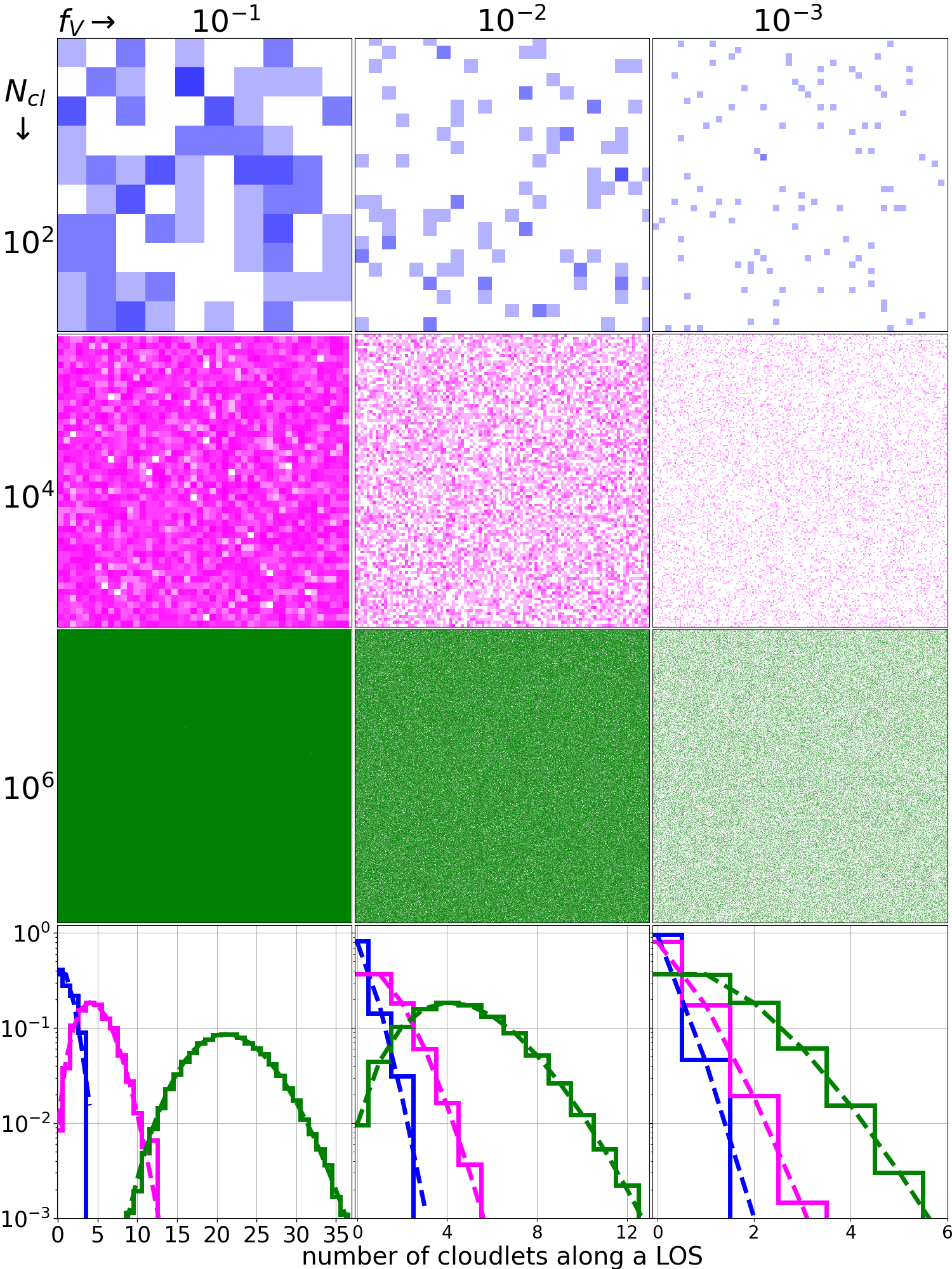
Figure 2: Projected cloud distribution (top 3$\times$3 panels) in a cubical volume with $N_{\rm cl}$ cubical cloudlets uniformly covering a volume fraction $f_{V}$. The size of vacancies equals the cloudlet size. As expected from simple estimates, the area covering fraction becomes order unity when $N_{\rm cl}\gtrsim f_{V}^{-2}$. The panels farther from the diagonal (toward the bottom-left) are deeper into the misty limit. The bottom panels show the normalized histogram of the number of cloudlets along different sightlines. The histogram is very well fit by a Poisson distribution (fits shown by dashed lines) with a mean $f_{V}^{2/3}N_{\rm cl}^{1/3}$. Note that the number of sightlines with zero and unity cloudlets becomes comparable for $N_{\rm cl}\sim f_{V}^{-2}$. This corresponds to the approach toward the mist limit with a unity area covering fraction.

To test the above scaling borrowed from D24, we carry out a simple Monte Carlo experiment (see Figure 2). We divide a uniform cubical volume $L^{3}$ into equal cells of size $l=Lf_{V}^{1/3}N_{\rm cl}^{-1/3}$ of our cubical cloudlets. $N_{\rm cl}$ cloudlets, which occupy a volume fraction $f_{V}$ of the available volume, fill these available cells with uniform probability. In this arrangement, either the cell is fully occupied or unoccupied (there is no partial occupation). The number distribution of cloudlets along a LOS is Poisson, with a mean $f_{V}^{2/3}N_{\rm cl}^{1/3}$ and a standard deviation equaling the square root of the mean (as expected for a Poisson distribution). A Poisson distribution is expected for a uniform cloud distribution. These mist estimates provide a useful benchmark to compare with more sophisticated models.

2.1.1 Terminal velocity of cloudlets within a CC

We can estimate the terminal velocity of a cloudlet within a CC by balancing the gravitational force and the drag force experienced by a cloudlet. The standard expression in the Rayleigh/turbulent drag regime is given by

$$v_{\rm term}^{\rm cl}=\sqrt{\frac{4\chi r_{\rm cl}}{3C_{D}R_{\rm CGM}}}v_{c}$$

$$\approx 80~{}{\rm km~{}s}^{-1}\left(\frac{\chi}{100}\right)^{1/2}\left(\frac{r_{\rm cl}/R_{\rm CGM}}{10^{-3}}\right)^{1/2}\left(\frac{v_{c}}{220~{}\rm kms^{-1}}\right),$$ (1)

where $\chi\approx 100$ is the density contrast between the cold and hot CGM phases, $C_{D}\sim 1$ is the drag coefficient, and $v_{c}\approx 220$ km s^-1 is the circular velocity of a Milky Way-like galaxy. For $r_{\rm cl}=100$ pc (best resolution achievable by current cosmological galaxy formation simulations) and $R_{\rm CGM}=100$ kpc, the above expression gives a terminal velocity $\sim 80$ km s^-1, much higher than the turbulent velocity across a CC ($\sim 16.5$ km s^-1; c.f. section 2.4). For cloudlets to be suspended in the CGM, and for mist description to be appropriate (as motivated by observations), the cloudlet terminal velocity should be $\lesssim 10$ km s^-1 (turbulent velocity within a CC), or the cloudlet size should be $\lesssim$ a few pc! This simple argument emphasizes the importance of phenomenological models like ours, given the computational intractability of modeling realistic suspended CGM cloudlets from first principles.

2.2 Analytical estimates

Before analyzing the Monte Carlo realization of CCs spread across the CGM, it is useful to present some analytic estimates to which the former can be compared.

Symbol	Meaning
$R_{\rm CGM}$	Radius of CGM
$R_{\rm CC}$	Radius of a cloud complex
$R_{\perp}$	Impact parameter
$M_{\rm cold}$	Total cold gas mass in the CGM
$M_{\rm CC}$	Mass of a cloud complex
$N_{\rm CC}$	Number of cloud complexes in the CGM
$N_{\rm cl}$	Number of cloudlets in a CC
$r_{\rm cl}$	Radius of a cloudlet
$f_{A}^{\rm CC}$	Area covering fraction of CCs in CGM
$f_{A}^{\rm cl}$	Area covering fraction of cloudlets in a CC
$\langle N_{\rm CC,LOS}\rangle$	Average number of CCs intersected along a sightline
$\langle N_{\rm ion}\rangle$	Average column density of an ion along a sightline
$f_{\rm V}$	Volume filling fraction of cold gas in a CC
$f_{\rm V}^{\rm CC}$	Volume filling fraction of CCs in CGM
$n_{\rm cold}$	Physical number density of cold gas
$\langle n_{\rm gas}\rangle$	Average density of gas in a misty CC
$\langle n_{\rm CC}\rangle$	Average number density of CCs
$\langle n_{\rm ion}\rangle$	Average number density of an ion
$b_{\rm thermal}$	Thermal broadening
$b_{\rm turb,CC}$	Turbulent broadening across a CC
$b_{\rm tot}$	Total broadening
$W_{2796}$	Equivalent Width of MgII
$v_{\rm LOS}$	LOS velocity

Table 1: Symbols used in this paper and their description.

2.2.1 Uniform distribution of cloud complexes

We begin with a uniform distribution of CCs in the CGM. In this case, the average number density of CCs is $\langle n_{\rm CC}\rangle=3N_{\rm CC}/(4\ \pi R_{\rm CGM}^{3})$, where $R_{\rm CGM}$ is the CGM radius. The average number of CCs intersected along a given LOS at an impact parameter $R_{\perp}$ is

$$\langle N_{\rm CC,LOS}\rangle(R_{\perp})=2\int_{0}^{s_{\rm max}}\langle n_{\rm CC}\rangle\pi R_{\rm CC}^{2}ds,$$ (2)

where $ds$ is the line element along the LOS and $s_{\rm max}=\sqrt{R_{\rm CGM}^{2}-R_{\perp}^{2}}$. This trivial integral gives the average number of CCs encountered along a LOS,

$$\langle N_{\rm CC,LOS}\rangle(R_{\perp})=\frac{3N_{\rm CC}R_{\rm CC}^{2}}{2R_{\rm CGM}^{3}}\sqrt{R_{\rm CGM}^{2}-R_{\perp}^{2}}.$$ (3)

The area covering fraction of CCs in a CGM starts to approach unity when the average number of CCs along a LOS exceeds unity, i.e., $\langle N_{\rm CC,LOS}\rangle\gtrsim 1$. For fiducial parameters ($R_{\rm CC}=10$ kpc, $R_{\rm CGM}=280$ kpc), this happens when $N_{\rm CC}\gtrsim 1000$. The average column density of an ion is

$$\langle N_{\rm ion}\rangle(R_{\perp})=2\int_{0}^{s_{\rm max}}(\langle n_{\rm CC}\rangle\pi R_{\rm CC}^{2}ds)(\langle n_{\rm ion}\rangle\langle L\rangle),$$ (4)

where the terms in the first bracket represent the average number of CCs intersected and the terms in the second bracket represent the average column density of an ion from a single CC. Here $\langle n_{\rm ion}\rangle$ is the average number density of an ion in a CC, which is estimated from $\langle n_{\rm gas}\rangle$ using a conversion factor of $1.7\times 10^{-6}$ for MgII (using Mg abundance at one-third solar metallicity and MgII ion fraction in typical CGM conditions; see Appendix A); and $\langle L\rangle$ is the area-averaged path length across a CC,

$$\langle L\rangle=\frac{\int_{0}^{R_{\rm CC}}2\pi bdb\,2\sqrt{R_{\rm CC}^{2}-b^{2}}}{\int_{0}^{R_{\rm CC}}2\pi bdb}=\frac{4}{3}R_{\rm CC}.$$ (5)

Assuming $\langle n_{\rm ion}\rangle$ to be uniform throughout the CC, we get the following expression for the average column density of an ion along the LOS,

$$\langle N_{\rm ion}\rangle(R_{\perp})=2N_{\rm CC}\langle n_{\rm ion}\rangle\left(\frac{R_{\rm CC}}{R_{\rm CGM}}\right)^{3}\sqrt{R_{\rm CGM}^{2}-R_{\perp}^{2}}.$$ (6)

2.2.2 Power-law distribution of cloud complexes

Next, we use a power-law distribution of CCs as the function of $r$ of the form

$$\langle n_{\rm CC}\rangle(r)=n_{0}\left(\frac{r}{R_{\rm CGM}}\right)^{-\alpha},$$ (7)

where $\alpha$ is the power-law index and $n_{0}$ is obtained using the normalization condition $N_{\rm CC}=\int\langle n_{\rm CC}\rangle(r)4\pi r^{2}dr$. We get the following expressions for the average number of CCs intersected and the column density of an ion along a LOS at an impact parameter $R_{\perp}$,

$$\langle N_{\rm CC,LOS}\rangle(R_{\perp})=2n_{0}\pi R_{\rm CC}^{2}R_{\rm CGM}^{\alpha}\int_{R_{\perp}}^{R_{\rm CGM}}\frac{r^{-\alpha+1}}{\sqrt{r^{2}-R_{\perp}^{2}}}\,dr,$$ (8)

and

$$\langle N_{\rm ion}\rangle(R_{\perp})=\frac{8}{3}\langle n_{\rm ion}\rangle n_{0}\pi R_{\rm CC}^{3}R_{\rm CGM}^{\alpha}\int_{R_{\perp}}^{R_{\rm CGM}}\frac{r^{-\alpha+1}}{\sqrt{r^{2}-R_{\perp}^{2}}}\,dr.$$ (9)

In addition to the average columns above, we also calculate the standard deviation using estimates derived in Appendix B.

2.2.3 Volume & mass fraction of cold gas in CCs

The mass fraction of CGM in the cold ($\sim 10^{4}$ K) phase is subdominant compared to the volume-filling hot phase (e.g., D24, Faerman & Werk 2023). The volume fraction is even smaller, since cold gas is denser. Table 3 in D24 quotes a cold mass fraction of 11.9% and a volume fraction of 0.16% for a Milky Way-like TNG50 halo. Since in our CC model, cold gas is confined only within CCs, we expect the volume and mass fraction of cold gas within a CC to be higher than the whole CGM.

The volume fraction of cold gas within a CC is

$$f_{V} = \frac{M_{\rm cold}}{N_{\rm CC}\mu m_{p}n_{\rm cold}(4\pi R_{\rm CC}^{3}/3)}=0.016\left(\frac{M_{\rm cold}}{10^{10}\ M_{\odot}}\right)$$ (10)

$$\times\left(\frac{N_{\rm CC}}{10^{3}}\right)^{-1}\left(\frac{n_{\rm cold}}{10^{-2}\,\rm cm^{-3}}\right)^{-1}\left(\frac{R_{\rm CC}}{10\,\rm kpc}\right)^{-3},$$

and the mass fraction is,

$$f_{M}=\frac{M_{\rm CC}}{M_{\rm CC}+(1-f_{V})\mu m_{p}n_{\rm hot}(4\pi R_{\rm CC}^{3}/3)},$$ (11)

which equals $0.62$ for our fiducial parameters (assuming $n_{\rm hot}=10^{-4}$ cm^-3 for hot gas in pressure equilibrium with cold clouds). As expected, the volume and mass fraction of cold gas within CCs is much higher than in the full CGM. The volume fraction of CCs within the CGM is

$$f_{V}^{\rm CC}=N_{\rm CC}\left(\frac{R_{\rm CC}}{R_{\rm CGM}}\right)^{3}=0.05\left(\frac{N_{\rm CC}}{10^{3}}\right)\left(\frac{R_{\rm CC}}{10\rm\,kpc}\right)^{3}\left(\frac{R_{\rm CGM}}{280\rm\,kpc}\right)^{-3}.$$ (12)

However, the volume fraction of cold gas in the CGM would be tiny, $f_{V}^{\rm CC}\times f_{V}\approx 0.08$%, consistent with Table 3 of D24 based on a Milky Way-like TNG50 halo. The volume fraction of CCs is typically small yet the area covering fraction can be substantial because of projection along the LOS (e.g., see Figure 1). This also means that the probability for overlap of two CCs is small ($\sim 5$%), implying that such overlapping CCs do not affect our statistics (also verified numerically for cloudlets within CCs in H23). Therefore, we do not bother about ensuring that CCs do not overlap. Similarly, the probability for the overlap of cloudlets within a CC is small since the volume fraction of cloudlets within a CC is also small (Eq. 10).

2.3 Comparing MgII column density with observations

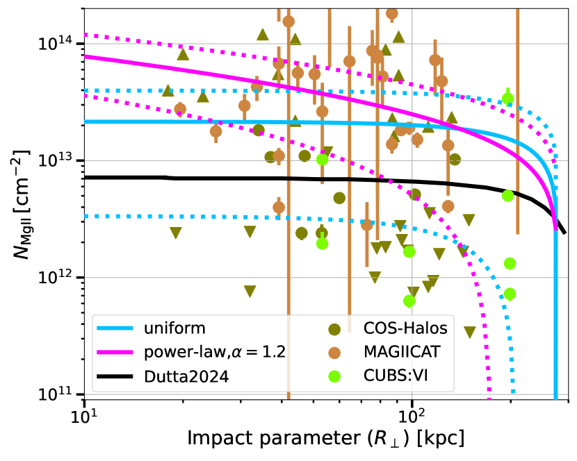
Figure 3: MgII column density as a function of impact parameter ($R_{\perp}$). The blue and magenta solid lines show the average MgII column density for uniform and power-law (power-law index $\alpha=1.2$) distribution of CCs in the CGM (Eqs. 6, 9). The dotted lines in the respective color show the expected standard deviation (see Appendix B) from the average column density. We adopt $M_{\rm cold}=10^{10}\,\rm M_{\odot}$, $N_{\rm CC}=10^{3}$, $R_{\rm CC}=10$ kpc, and $R_{\rm CGM}=280$ kpc to generate these profiles. The solid black line shows the baseline column density predicted by D24, which uses somewhat different parameter values. COS-Halos (Werk et al. 2013), MAGiiCAT (Nielsen et al. 2016), and CUBS (Qu et al. 2023) data points are shown in different colors with the upper (lower) triangles showing the lower (upper) limits.

Figure 3 shows the expected average column density of MgII as a function of the impact parameter ($R_{\perp}$) for a uniform distribution of CCs in solid blue (Eq. 6) and for a power-law distribution (power-law index $\alpha=1.2$) in solid magenta (Eq. 9). The dotted lines in respective colors show the expected spread (standard deviation) in column density (see Eq. 21), which is computed by taking care of the variation in the number of CCs along a LOS and the deviation in the intersected length of a CC. The solid black line shows the baseline column density value predicted by D24 based on their one-zone model of the CGM in the mist limit. We adopt $M_{\rm cold}=10^{10}\,\rm M_{\odot}$, $N_{\rm CC}=10^{3}$, $R_{\rm CC}=10$ kpc, $R_{\rm CGM}=280$ kpc as our fiducial parameters. We choose the parameters similar to (but not identical to; in particular, our CGM extent of $280$ kpc is smaller than their choice of $333$ kpc) what D24 found for one of the Milky Way-like TNG50 halos. Plotted along with are the observations from COS-Halos (Werk et al. 2013), MAGiiCAT (Nielsen et al. 2016), and CUBS (Qu et al. 2023) surveys covering roughly $\sim 10^{11}-10^{13}M_{\odot}$ in halo mass. The circles show detections, while the upper and lower triangles show the lower and upper limits, respectively. These column densities are typically obtained from the total equivalent width along a LOS derived from the normalized absorption spectra (see section 2.4). For the CUBS data, we plot the column density of each component along a LOS, rather than summing the column densities of the components along the LOS. Notice a larger scatter in the observed values at similar impact parameters. Our analytical expressions (Eqs. 6, 9) pass through the general scatter of the observations. The average column density does not provide stringent constraints on the distribution of CCs because of a large spread in the observationally inferred MgII column density. Also, we see many upper and lower limits in the observed data. This large scatter motivates our misty CC model.

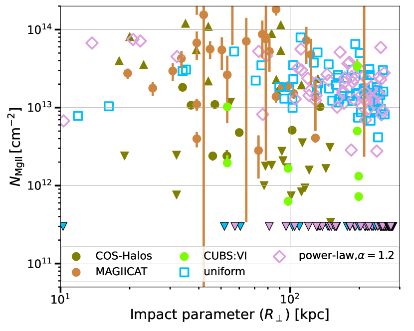
Figure 4: Blue square and magenta diamond points are the $100$ randomly selected sightlines (with larger LOSs at larger $R_{\perp}$) from $10^{4}$ sightlines uniformly spaced in $\log_{10}R_{\perp}$. The green, brown, and light green points are the observations from the COS-Halos, MAGiiCAT, and CUBS surveys, respectively. Note that we also mark the upper limit (column density less than $3\times 10^{11}\,\rm cm^{-2}$ close to the lowest value from the COS-Halo survey) shown with blue and magenta lower triangles along the sightlines with no intersected CCs. The large scatter in column density is produced by distributing cold gas in CCs rather than by distributing cold gas uniformly in the entire CGM.

To compare the spread of observed MgII column densities with the model, we create a Monte Carlo realization of $10^{4}$ sightlines from our misty CC model. Figure 4 shows MgII column density for $100$ randomly selected LOSs from $10^{4}$ LOSs. The blue square and magenta diamonds show the MgII column density for uniform and power-law distributions, respectively. The observed data points are from the COS-Halos (Werk et al. 2013), MAGiiCAT (Nielsen et al. 2016), and CUBS (Qu et al. 2023) surveys. We also show the upper limit from our model (no CCs intersected along these sightlines) using blue and magenta lower triangles. We adopted the upper limit for MgII at the column density of $3\times 10^{11}\,\rm cm^{2}$, which is the lowest upper limit from the COS-Halo survey (green lower triangles). The large scatter in the observed column density values at approximately the same impact parameter is well reproduced by limiting the cold gas to misty CCs rather than filling the entire CGM in the mist limit (D24).

The inner CGM has a higher pressure and density compared to the outskirts. Because of this, the MgII fraction (and hence MgII column density) is expected to be higher by a factor of $\sim 3$ in the inner CGM and lower by a similar factor at large radii (see Figure 18). We use a fixed MgII abundance fraction independent of radius in all our models presented in this section. We allow the physical density of the gas and hence MgII abundance to vary with radius in Figure 16, where we are able to better match the observed scatter of MgII column densities.

Column density is typically derived from the Equivalent Width (EW) based on Voigt profile modeling of various absorption components produced by the CGM in the background quasar continuum. Therefore, in the next section, we compute EWs for both uniform and power-law CC distribution and compare them with the observed EW, which is the direct observable in absorption line studies.

2.4 Computing Equivalent Width

We can compute the EW using the column density estimated above using the curve of growth and assuming a reasonable $b$-parameter (that characterizes the thermal and turbulent broadening of the absorption line; Draine 2011). For a MgII column density $\gtrsim 10^{13}$ cm^-2, the EW will be lower than linear extrapolation of the flat portion of the curve of growth (see Figure 5). For example, if we have $10$ CCs (coinciding in LOS and turbulent velocities so that they produce a single absorption feature) along a LOS, each with a MgII column density $\sim 10^{13}\,\rm cm^{-2}$, then the EW computed using the total column density will be lower than the sum of EWs computed for each CC individually. But summing the EWs is appropriate when the LOS CCs are kinematically non-overlapping. The correct EW along a LOS lies between these two extremes and depends on the details of LOS velocities of cloud complexes, as we discuss later.

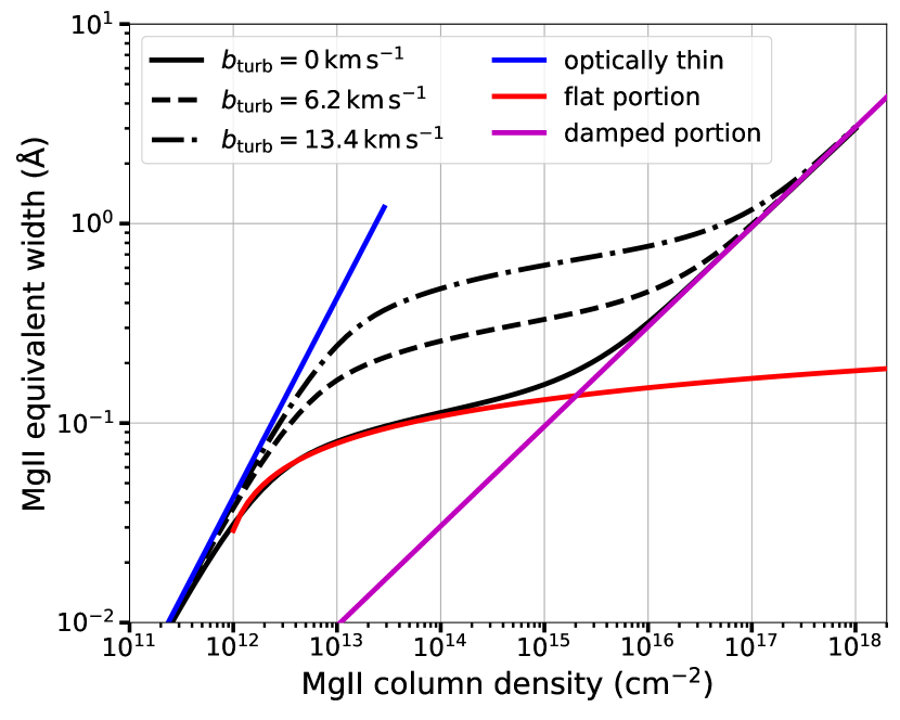
Figure 5: Variation in MgII EW with MgII column density. The black lines show the EW for various $b_{\rm turb}$ values calculated using absorption profiles. The solid blue, red, and magenta lines show the analytical relation between EW and column density in the optically thin limit, flat portion, and damped portion of the curve of growth. These analytic relations are from Draine (2011) (see Chapter 9). We assume thermal broadening at $T=10^{4}$ K for MgII, which gives $b_{\rm thermal}=2.6\,\rm km\,s^{-1}$. In the flat portion (applicable to most of our CCs, see Fig. 4), the EW increases with increasing turbulent broadening.

To compute the EW of the individual CCs intersected along a LOS, we populate $N_{\rm CC}$ CCs each of radius $R_{\rm CC}$ in the CGM for both uniform and power-law distributions. For a uniform distribution, we obtain the $x,y,z$ coordinates of the CC centers by drawing a random number from a uniform distribution between $-R_{\rm CGM}$ and $R_{\rm CGM}$ independently in $x,y,z$ directions. For power-law distribution with index $\alpha$, we first sample the radial distance $r$ of the center of CC from the power-law distribution (see Eq. 7). We then draw a uniform deviate in $\phi$ ranging from $0$ to $2\pi$ and in $\cos\theta$ from $-1$ to $1$. Using these $r,\phi$ and $\theta$, we compute the $x,y,z$ coordinates. We ensure that the CCs are not populated beyond $R_{\rm CGM}$ by recomputing the CC coordinates in case they are.

After generating the centers of CCs, we shoot $10^{4}$ LOSs (spaced uniformly in $\log_{10}R_{\perp}$) through the CGM in the $z$ direction. We then compute the $x,y$ coordinates of the LOS by drawing a random value of $\phi$ uniformly between $0$ and $2\pi$. We then calculate the number of CCs intersected and the corresponding intersected length along each LOS. We calculate the column density of MgII from each intersected CC by using a conversion factor of $1.7\times 10^{-6}$ (roughly corresponding to the cold gas density of $\approx 0.01$ cm^-3; see Appendix A) to convert the cold gas density in CC ($n_{\rm cold}$) to the number density of MgII. Recall that our CCs are assumed to be in the misty limit.

Ansatz for turbulent velocity across a CC: To compute EW, we consider both thermal broadening and turbulent broadening across a CC. We assume the temperature of the cold gas to be $10^{4}$ K, which gives thermal broadening of $b_{\rm thermal}=\sqrt{k_{B}T/(Am_{p})}=2.6\rm\,km\,s^{-1}$ for MgII. We also consider the contribution of turbulent broadening ($b_{\rm turb,CC}$; across a CC) for each CC. We compute $b_{\rm turb,CC}$ in the following way. Assuming that turbulence is driven at CGM global scales with velocity dispersion $\sigma_{\rm turb,CGM}$ that cascades down to CC scale without loss, the velocity dispersion at CC scale is given by $\sigma_{\rm turb,CC}=\sigma_{\rm turb,CGM}\times(R_{\rm CC}/R_{\rm CGM})^{1/3}$. Therefore, the total broadening is $b_{\rm tot}=\sqrt{b_{\rm thermal}^{2}+b_{\rm turb,CC}^{2}}$ (in the micro-turbulent limit, Mihalas 1978), where $b_{\rm turb,CC}=\sqrt{2}\sigma_{\rm turb,CC}$. To estimate $\sigma_{\rm turb,CGM}$, we assume the turbulent Mach number of the hot ($\sim 10^{6}$ K), volume-filling CGM to be $\sim 0.4$ (e.g., Schmidt et al. 2021; Mohapatra et al. 2022b). These assumptions give $\sigma_{\rm 3Dturb,CGM}\approx 50\rm\,km\,s^{-1}$. For $R_{\rm CC}=10$ kpc and $R_{\rm CGM}=280$ kpc, we get $\sigma_{\rm 3Dturb,CC}=16.5\rm\,km\,s^{-1}$. Thus, the 1D turbulent dispersion is $\sigma_{\rm turb,CC}=\sigma_{\rm 3Dturb,CC}/\sqrt{3}=9.5\rm\,km\,s^{-1}$. For simplicity, we choose the turbulent broadening parameter to be the same for all impact parameters across the CC. Fig. 7 from H23 shows that only the largest EWs are slightly enhanced by increasing the turbulent velocity across a CC beyond $8$ km s^-1.

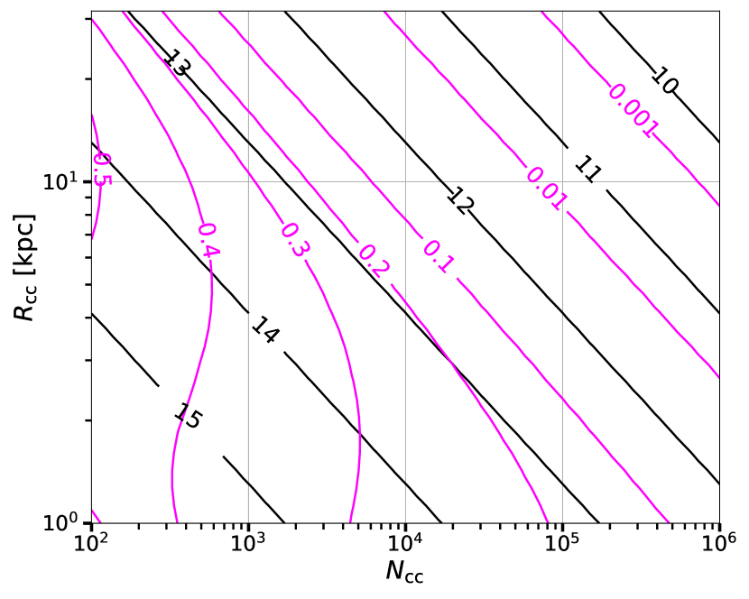
Figure 6: Contours of equal (in log₁₀) maximum MgII column density (corresponding to LOS passing through the center of CC; black lines) and equivalent width (magenta lines, in units of $\rm\mathring{A}$) in the parameter space of $N_{\rm CC}$ and $R_{\rm CC}$ for a single cloud complex. For MgII column densities $\gtrsim 10^{13}$ cm^-2, the EW saturates in the flat part of the curve of growth (see Figure 5) and the curves of constant EW are no longer parallel to the constant column density contours. The EW increases with $R_{\rm CC}$ for a fixed MgII column density because of a larger $b_{\rm turb,CC}$ (see Fig. 5).

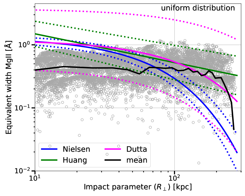
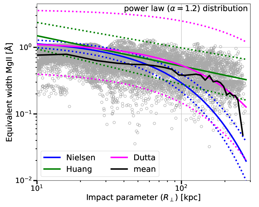
Figure 7: MgII EW as a function of impact parameter. The left and right panels are for the uniform and power-law distribution of CCs in the CGM. The grey scattered points (note that empty sightlines are not shown) show the total MgII EW as a function of the impact parameter for $10^{4}$ sightlines. We use the fiducial parameters $M_{\rm cold}=10^{10}\ M_{\odot}$, $R_{\rm CGM}=280$ kpc, $N_{\rm CC}=10^{3}$, and $R_{\rm CC}=10$ kpc. The black solid line shows the mean of grey points in each $10$ kpc bin. The blue, green, and magenta lines show the best-fit relation between MgII EW and impact parameter from Nielsen et al. (2013), Huang et al. (2021), and Dutta et al. (2020) respectively. The corresponding dotted colored lines show the $1\sigma$ uncertainties. Note that the scatter in the observed EW is well produced by both the uniform and power-law distribution, but the observations slightly better match the power-law distribution.

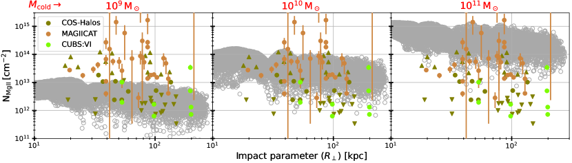
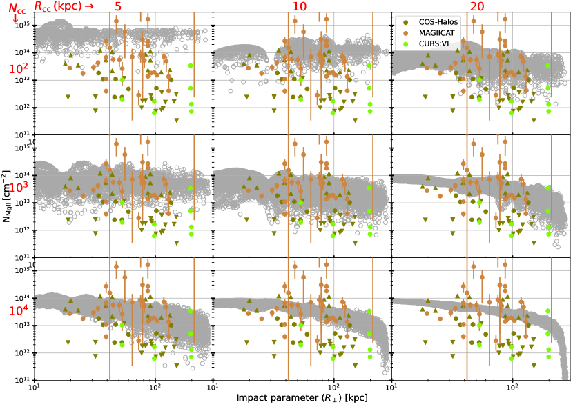
Figure 8: Variation in the MgII column density along $10^{4}$ sightlines with the cold gas mass, number of CCs, and radius of CCs for a power-law ($\alpha=1.2$) distribution of CCs in the CGM. Only non-zero values are shown with circles, resulting in a smaller number of them when the covering fraction is small. It is evident from the top panels that cold CGM mass of $\sim 10^{10}\,M_{\odot}$ best matches the observed data. The bottom $3\times 3$ panels show the variation in MgII column density with $R_{\rm CC}$ and $N_{\rm CC}$ for a fixed cold gas mass of $10^{10}\,M_{\odot}$. Notice that the increase in the size of CC results in less scatter in the column density because with a larger CC, the volume fraction of CCs is larger, and a similar number of CCs intersected along different sightlines. A similar trend is observed for a larger number of CCs in the CGM. It is clear that $10^{3}$ CCs with $R_{\rm CC}=10$ kpc and $M_{\rm cold}=10^{10}M_{\odot}$ best explain the observed MgII column density distribution.

Figure 6 shows the contour plot of maximum MgII column density (black lines indicate ${\rm log}_{10}N_{\rm MgII}$; corresponding to the LOS passing through the center of a CC) and equivalent width (in $\rm\mathring{A}$; magenta lines) in the $N_{\rm CC}-R_{\rm CC}$ parameter space for a single CC for a fixed total cold gas mass $M_{\rm cold}=10^{10}\,\rm M_{\odot}$. The MgII column density through the center of CC is given by

$$N_{\rm MgII,max}=1.7\times 10^{13}\ {\rm cm^{-2}}\left(\frac{M_{\rm cold}}{10^{10}\ M_{\odot}}\right)\left(\frac{N_{\rm CC}}{10^{3}}\right)^{-1}\left(\frac{R_{\rm CC}}{10\rm kpc}\right)^{-2}.$$ (13)

To compute the EW, we first generate the normalized absorption profile ($I_{\nu}=\exp[-\tau_{\nu}]$, where $\tau_{\nu}\propto N_{\rm MgII}$ is the frequency-dependent optical depth; see Eq. 9.5 in Draine 2011) and then compute the area under the normalized absorption profile as the definition of EW. In the linear regime of the curve of growth ($N_{\rm MgII}\lesssim 10^{12}\,\rm cm^{-2}$; see Fig. 6), the EW and column density contours run parallel to each other, which suggests a single value of EW for a given value of column density (Eq. 13). As we move to higher column density $N_{\rm MgII}\gtrsim 10^{13}\,\rm cm^{-2}$, for a fixed column density the EW increases with an increase in $R_{\rm CC}$ as $b_{\rm turb,CC}$ is larger for a larger CC according to our ansatz for CGM turbulence (see Figure 5). This regime lies in the flat part of the curve of growth.

Ansatz for LOS velocity of a CC: To compare with the observed EW distribution, we need the LOS velocities of the intersected CCs. We assign a 3D velocity field with a Gaussian distribution and a Kolmogorov power spectrum ($v_{l}\propto l^{1/3}$) on a 600³ grid across the entire CGM. Every CC is assigned the velocity from the closest grid cell. The turbulent velocity field has zero mean and standard deviation $\sigma_{\rm 3Dturb,CGM}=50\rm\,km\,s^{-1}$ (assuming our ansatz for global CGM turbulence). In addition to this bulk velocity, each CC also has a Gaussian spread in its internal velocities ($\sigma_{\rm turb,CC}$), as mentioned earlier. To generate the absorption profile along each LOS, we consider the blending of absorption profiles from all intersected CCs. The optical depth along a LOS is computed as the sum of the optical depths from each intersected CC, $\tau(\nu)=\sum_{i}\tau_{i}(\nu)$, where the summation goes over all the intersected CCs. Thus, the normalized absorption profile is given as $I(\nu)=\exp[-\tau(\nu)]$ and the area under it gives the EW along a LOS.

2.5 Comparing Equivalent Width with MgII observations

There are various observational estimates of MgII EW ($W_{2796}$). Performing an extensive literature survey, Nielsen et al. (2013) compiled the MAGiiCAT database with 182 galaxies towards 134 quasar lines of sight. The galaxies reside at intermediate redshift range $0.07\leq z\leq 1.1$ with a median of $0.359$ and B-band luminosities of $0.02\leq L_{\rm B}/L_{\rm B}^{*}\leq 5.87$ with a median of $0.611$. They identified all the galaxies to be isolated, as they do not have any neighbors within the projected distance of $100$ kpc and a velocity offset smaller than $500\,\rm km\,s^{-1}$. The range in impact parameter is $5.4\leq R_{\perp}\leq 194$ kpc with a median of $49$ kpc. They fitted the EW ($2796$) and impact parameter data with a log-linear relation and the best-fit values and $1\sigma$ uncertainties are

$$\mathrm{log}\,W_{2796}(\mathring{\rm A})=0.27\pm 0.11+(-0.015\pm 0.002)R_{\perp}.$$ (14)

Dutta et al. (2020) used the MUSE Analysis of Gas around Galaxies (MAGG) survey to analyze the MgII absorbing system. Their galaxies span a range in redshift $0.8-1.5$ and a range in halo mass of $9\times 10^{9}-4\times 10^{14}\,M_{\odot}$ with a median halo mass $6\times 10^{11}\,M_{\odot}$. Their best-fit relation between $W_{2796}$ and impact parameter along with stellar mass ($\rm M^{*}_{\odot}$ in units of solar mass) is

$$\mathrm{log}\,W_{2796}(\mathring{\rm A}) =-0.61^{+0.63}_{-0.58}+(-0.008^{+0.003}_{-0.004})R_{\perp}$$ (15)

$$+\,0.53^{+0.34}_{-0.28}\times(\rm log\,M^{*}_{\odot}-9.3).$$

More recently, Huang et al. (2021) analyzed multiple surveys to report the properties of the MgII absorbing systems. They found $211$ isolated galaxies with impact parameters $9-497$ kpc with a median of $94$ kpc. They cover a redshift range of $0.1-0.48$ with a median of $0.21$. These galaxies span a wide range in stellar mass of $2\times 10^{8}-4\times 10^{11}\,M_{\odot}$ with a median stellar mass of $4\times 10^{10}\,M_{\odot}$. They fitted the log-log relation to $W_{2796}$ versus the impact parameter and found the best-fit values to be

$$\mathrm{log}\,W_{2796}(\mathring{\rm A}) =(1.35\pm 0.25)-(1.05\pm 0.17)\mathrm{log}\,R_{\perp}$$ (16)

$$+(0.21\pm 0.08)\times(\rm{log}\,M^{*}_{\odot}-10.3).$$

All the above works quote a single EW, corresponding to the area under the absorption spectrum across velocities, for each LOS and do not separate different components along a LOS.

Figure 7 shows the MgII EW for the uniform (left panel) and power-law (right panel) distribution of CCs. The grey scatter points show the Monte Carlo simulated data with LOSs intersecting a range of lengths along each CC; empty sightlines are not shown. The solid black line shows the mean of the grey points. The observed relation of EW with impact parameter ($R_{\perp}$) from Nielsen et al. (2013), Huang et al. (2021), and Dutta et al. (2020) are shown using blue, green, and magenta solid lines, respectively. The dotted lines in the respective colors show the $1\sigma$ uncertainties. We use $M^{*}_{\odot}=6.08\pm 1.14\times 10^{10}$ (in Eq. 15) for the Milky Way (Licquia & Newman 2015). We adopt the fiducial parameters $M_{\rm cold}=10^{10}\,\rm M_{\odot}$, $R_{\rm CGM}=280$ kpc, and $N_{\rm CC}=10^{3}$. It is evident from the figure that the power-law distribution of CCs produces a better fit to the observed relation than the uniform distribution.

2.6 Estimating cold gas mass in the CGM

One of the fundamental physical properties of the CGM is its mass distribution across different temperature phases. While the volume-filling hot phase is difficult to observe, quasar absorption lines from cold and warm CGM ions are commonly observed. However, there are large variations in the inferred column densities and several upper and lower limits (e.g., see Fig. 3). Because of these wild variations, it is hard to estimate the cold and warm gas masses. The large variations, scatter, and upper and lower limits in the column density carry important information that can help us infer the physical properties of the cold/warm CGM.

The top panels of Figure 8 show the column density distribution along 10⁴ sightlines (empty sightlines are not shown) across the CGM with 10³ CCs and a CC radius $R_{\rm CC}=10$ kpc, but with the cold gas mass of 10⁹, 10¹⁰ and 10${}^{11}M_{\odot}$. We only show the distribution for the power-law $\alpha=1.2$ model (a uniform distribution gives similar trends). The average MgII column density varies linearly with the cold gas mass. This suggests that the column density distribution of cold gas tracers (like MgII) is a quantitative indicator of the cold gas mass in the CGM. The observed spread in MgII column density is most consistent with a cold CGM mass $\sim 10^{10}M_{\odot}$. The distribution of MgII column density from our Monte Carlo-generated LOSs is too small (large) for $10^{9}~{}(10^{11})M_{\odot}$ in the cold CGM.

The bottom $3\times 3$ panels of Figure 8 show the variation of MgII column density for cold CGM mass of $10^{10}M_{\odot}$ but with a variation of the number of CCs ($N_{\rm CC}$ across rows) and the CC radius ($R_{\rm CC}$ across columns). For small $R_{\rm CC}$ and $N_{\rm CC}$, the detected column densities are much larger, but the covering fraction is small since most sightlines do not encounter cold gas. Since we only show detections, the cases with a small covering fraction will have a smaller number of grey circles. For larger $R_{\rm CC}$, the covering fraction increases, and the individual LOS column densities are smaller. With an increasing number of CCs and CC sizes (bottom right panels), the scatter in MgII column density decreases. The observed spread in the inferred column densities of cold/warm gas can thus help us constrain cold CGM parameters such as $M_{\rm cold}$, $N_{\rm CC}$, and $R_{\rm CC}$. The best fit is obtained for $N_{\rm CC}=10^{3}$, $R_{\rm CC}=10$ kpc and $M_{\rm cold}=10^{10}M_{\odot}$.

2.6.1 Relation between average column density & covering fraction

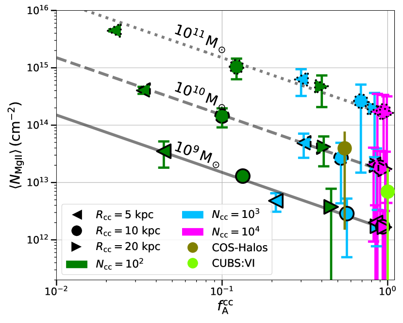
Figure 9: The average MgII column density as a function of the area covering fraction of CCs for various combinations of the cold gas mass, $N_{\rm CC}$ and $R_{\rm CC}$ (see Figure 8). The points with solid, dashed, and dotted black lines on their borders are for a cold gas mass of $10^{9}$, $10^{10}$, and $10^{11}\,M_{\odot}$ respectively. The error bars on each point show the standard deviation on the column densities. The dotted, dashed, and solid black lines show the contours of constant average MgII column density times the covering fraction for three different values $\langle N_{\rm mgII}\rangle\times f_{\rm A}^{\rm CC}=10^{12.2},10^{13.2}$, and $10^{14.2}$ cm^-2, respectively. The product of these two quantities can be used to constrain the cold gas mass in the CGM. To compute the above quantities, we selected $100$ random sightlines (so that the probability of selection is proportional to the area of the projected CGM annulus) out of $10^{4}$ to be statistically consistent with the observations. The green and light green points represent data from the COS-Halos (Werk et al. 2013) and CUBS (Qu et al. 2023) surveys, respectively (we do not include MAGiiCAT data here because of anomalously large column densities and error bars). The errors in the estimation of individual column densities are small, but the scatter (indicated by 1-$\sigma$ variation) is large. The positions of these data points indicate a cold gas mass of $\sim 10^{10}\,\rm M_{\odot}$ for both data sets.

For the same cold CGM mass, the CCs can be arranged in different physical configurations – compact CCs with smaller $R_{\rm CC}$ or fewer CCs. With compact CCs and fewer of them, we expect to encounter several empty sightlines, resulting in a small covering fraction. But whenever a LOS encounters a CC in this case, it results in a large column density (e.g., compare the second-left column of Figure 8 with the bottom-left column). One can easily verify that the product of the average column density and the covering fraction is roughly the same for the same cold CGM mass. Figure 9 shows the correlation between the average MgII column density and the covering fraction of CCs in the CGM for various combinations of $R_{\rm CC}$, $N_{\rm CC}$, and $M_{\rm cold}$. We chose $100$ random samples (with selection probability proportional to the area of the annulus to which it belongs; see footnote 2) from a total of $10^{4}$ (see Figure 8) to be statistically consistent with observations and compute the average MgII column density and covering fraction for these. The points with solid, dashed, and dotted black lines on their borders correspond to the cold gas mass of $10^{9},10^{10}$, and $10^{11}\,\rm M_{\odot}$, respectively. The error bar shows the standard deviation in the column densities. The dotted, dashed, and solid black lines show the contours of a constant average column density times the covering fraction for the three cases with $\langle N_{\rm mgII}\rangle\times f_{\rm A}^{\rm CC}=10^{12.2},10^{13.2}$, and $10^{14.2}$. The points corresponding to the same cold CGM mass have a similar value of $\langle N_{\rm mgII}\rangle\times f_{\rm A}^{\rm CC}$, regardless of $R_{\rm CC}$ and $N_{\rm CC}$. The green and light green points show data from the COS-Halos (Werk et al. 2013) and CUBS (Qu et al. 2023) surveys, respectively. The positions of these data points indicate a cold gas mass of approximately $\sim 10^{10}\,\rm M_{\odot}$ for both data sets. For COS-Halos, we calculate the covering fraction by dividing the number of detected and lower-limit LOSs by the total number of observed sightlines. For the CUBS data, we choose the covering fraction to be unity and only include the LOSs where MgII is detected. A more accurate statistical analysis of the data is beyond the scope of our paper. Thus, the combination of the covering fraction and average column density can constrain the mass of the cold CGM. Moreover, the spread in column density distribution constrains the number of CCs and their sizes.

3 Cloudlets within a cloud complex

In the last section, we analyzed the distribution of misty CCs in the CGM. Apart from thermal broadening, we also incorporated the contribution of turbulent broadening across a CC in computing EW. In this section, we zoom in on a single CC, generate cloudlets within it, and assign turbulent velocity to each cloudlet. Here, we do not assume any turbulent broadening within a cloudlet, since turbulent broadening across a $\sim$ parsec size cloudlet is smaller than thermal broadening. Instead, turbulent broadening emerges due to the blending of absorption profiles of cloudlets intersected along a LOS, which are typically closely spaced in velocity space.

First, we populate $N_{\rm cl}=M_{\rm cold}/N_{\rm CC}$ cold cloudlets in a CC. We fix the mass of the CC to be $M_{\rm CC}=10^{7}\,\rm M_{\odot}$ (corresponding to our fiducial mCC parameters $M_{\rm cold}=10^{10}M_{\odot}$ and $N_{\rm CC}=10^{3}$) and assume the number density of cold gas within cloudlets to be $n_{\rm cold}=10^{-2}\,\rm cm^{-3}$. For simplicity, we assume the cloudlet radius $r_{\rm cl}=5$ pc. Therefore, the total number of cloudlets within a CC is

$$N_{\rm cl}=1.3\times 10^{8}\,\left(\frac{M_{\rm CC}}{10^{7}\,\rm M_{\odot}}\right)\left(\frac{n_{\rm cold}}{10^{-2}\rm\,cm^{-3}}\right)^{-1}\left(\frac{r_{\rm cl}}{5\rm\,pc}\right)^{-3}.$$ (17)

Recall that the mist limit (most sightlines passing through cold cloudlets) is achieved for $N_{\rm cl}\gtrsim f_{V}^{-2}$ (see Fig. 2), where $f_{V}$ is the volume fraction of cold gas within a CC. The volume fraction of cold gas for our fiducial CC model is $\approx 0.016$ (Eq. 10) and therefore $10^{8}$ cloudlets $\gg f_{V}^{-2}$ are safely in the mist limit. The maximum MgII column density estimated from a single CC is $1.7\times 10^{13}\,\rm cm^{-2}$ (see Eq. 13) for the CC of radius $10$ kpc. The maximum MgII column density from a single cloudlet of $r_{\rm cl}=5$ pc and cold gas number density of $10^{-2}\,\rm cm^{-3}$ is $\approx 5\times 10^{11}\,\rm cm^{-2}$ (assuming $f_{\rm MgII}=1.7\times 10^{-6}$). The above estimates suggest that there should be $\approx 34$ cloudlets along a LOS passing through the center of our CC to match the column density value in the mist limit case in the previous section. The number of cloudlets required along a LOS is even larger for a smaller $r_{\rm cl}$ ($\propto r_{\rm cl}^{-1}$ for a fixed column density).

In our Monte Carlo experiments with cloudlets, we populate a CC uniformly with $N_{\rm cl}$ cloudlets of a given size. We determine the $x,y,z$ coordinates of the cloudlets by drawing random numbers from a uniform distribution between $-R_{\rm CC}$ and $R_{\rm CC}$. We ensure that the cloudlets are within the CC by regenerating the coordinates of the cloudlets that lie outside the CC. Once we generate the coordinates of all cloudlets, we assign 3D turbulent velocity with Kolmogorov spectrum to each cloudlet similar to the previous section but over a grid of $200^{3}$ across the CC. The turbulent velocity field has zero mean and standard deviation $\sigma_{\rm 3Dturb,CC}=\sigma_{\rm 3Dturb,CGM}\times(R_{\rm CC}/R_{\rm CGM})^{1/3}=16.5\rm\,km\,s^{-1}$ for $R_{\rm CC}=10$ kpc and $R_{\rm CGM}=280$ kpc with $\sigma_{\rm 3Dturb,CGM}=50\,\rm km\,s^{-1}$ estimated in the previous section. Note that the smaller CCs have a smaller $\sigma_{\rm 3Dturb,CC}$, and therefore cloudlets are closely packed in the velocity space.

After assigning 3D turbulent velocity to all the cloudlets, we shoot $10^{4}$ sightlines through the CC (along $z$ direction). For each LOS, we determine the number of cloudlets intersected, the total intercepted cloudlet length, column density, and the LOS velocity of each intersected cloudlet. For a given LOS, we then obtain the absorption profile of MgII from all the individual intersected cloudlets. Note that we do not assume any non-thermal broadening across a cloudlet. We assume the temperature of the cold gas to be $10^{4}$ K which corresponds to $b_{\rm thermal}=2.6\,\rm km\,s^{-1}$ for MgII. To obtain the column density of MgII from the total column density (calculated using the intercepted cloudlet length), we use the conversion factor of $1.7\times 10^{-6}$, assuming a $1/3$ solar metallicity.

3.1 Turbulent broadening within a cloud complex

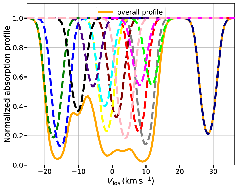
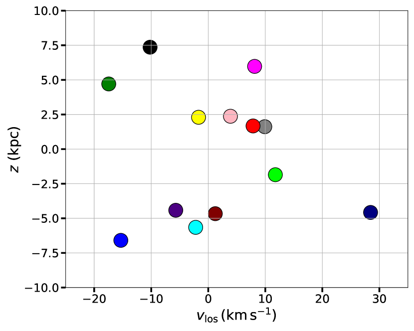
Figure 10: In the top panel, the dashed lines in different colors (total $13$) show the MgII absorption profile from individual cloudlets intersected along a LOS through a CC. The solid orange line shows the overall/total absorption profile from all the intersected cloudlets. We need $6$ absorbing components to fit the overall absorption profile. In the bottom panel, we show the $z$ coordinate and the LOS velocity of the intersected cloudlets. The color of the points corresponding to individual cloudlets is consistent with the top panel. The cloudlets close in velocity space need not be close in physical space and vice versa.

With column density, $b_{\rm thermal}$ and $v_{\rm LOS}$ (LOS velocity of the cloudlet), we obtain the MgII absorption profile for each intersected cloudlet along a LOS. We then calculate the overall/total absorption profile along a sightline. To do so, we calculate the total optical depth $\tau(\nu)=\sum_{i}\tau_{i}[\nu]$, where the summation goes over all the intersected cloudlets along a LOS. We then obtain the overall normalized absorption profile as $I(\nu)=\exp(-\tau(\nu))$. For example, the dashed lines in the top panel of Figure 10 with different colors show the individual MgII absorption profiles (total $13$) along a LOS with an impact parameter of $100$ pc from the center of the CC with $R_{\rm CC}=10$ kpc, $r_{\rm cl}=20$ pc. The solid orange line shows the overall absorption profile from all the intersected cloudlets. Depending on the LOS velocity of the intersected cloudlets, the absorption profiles may be blended. We then identify the number of absorbing components to be fitted to the overall absorption profile. In the overall profile (solid orange line in the top panel of Figure 10), which is generated using $13$ individual profiles, $6$ absorbing components are needed. We then fit the required number of absorbing components with individual Voigt profiles keeping the column density, $b_{\rm tot}=\sqrt{b_{\rm thermal}^{2}\,+\,b_{\rm turb}^{2}}$, and $v_{\rm LOS}$ as free parameters. We obtain $b_{\rm turb}$ from each absorbing component along a LOS as $b_{\rm thermal}$ is fixed to $2.6\rm\,km\,s^{-1}$. We do this exercise for all $10^{4}$ sightlines and obtain $b_{\rm turb}$ for all such absorbing components in the overall/total absorption spectra. Note that $b_{\rm turb}$ is zero for the cloudlet which is not blended. We do not include unblended absorption profiles with $b_{\rm turb}=0$ in our further analysis.

In the bottom panel of Figure 10, we show the $z$ coordinate of the intersected cloudlets along a given LOS (same as in the top panel) on the y-axis and the LOS velocity on the x-axis. The color of the points in the bottom panel is consistent with the absorption profile of the cloudlets in the top panel. The cloudlet shown with the dark blue point at $z\approx\hbox{-}5$ kpc and $v_{\rm LOS}\approx 30\,\rm km\,s^{-1}$ is not blended with other cloudlets as can be seen with the absorption profile in the top panel. The turbulent broadening of such cloudlets is zero. The two cloudlets around $v_{\rm LOS}\approx-15$ (green and blue points in the bottom panel) are blended, as can be seen with the overlapping absorption profiles in the top panel. These two cloudlets have a similar LOS velocity but are separated by $\approx 12$ kpc in physical space. This signifies that the cloudlets far away in physical space can be blended in velocity space. The two cloudlets which are around $v_{\rm LOS}\approx 10$ km s^-1 (red and grey points in the bottom panel) are close in both velocity and physical space and therefore are expected to blend as seen in the top panel.

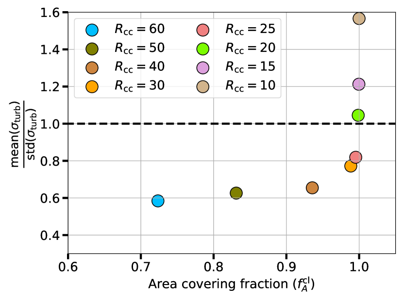
Figure 11: The ratio of the mean to the standard deviation of $\sigma_{\rm turb}$ the distribution (excluding $\sigma_{\rm turb}=0$ components) for various CC sizes (corresponding to $f_{A}^{\rm cl}$) and a fixed cloudlet radius $r_{\rm cl}=5$ pc. The $\sigma_{\rm turb}$ values are obtained for each absorbing component (in the overall absorption spectrum along a LOS) over $10^{4}$ LOSs. The horizontal dashed black line shows the mean-to-standard deviation ratio of $1$. Note that the mean becomes larger than the standard deviation when the area covering fraction starts to approach unity. The area covering fraction is larger for smaller CCs. An increasingly large number of cloudlets (for smaller $R_{\rm CC}$) along the LOS increases blending and leads to an increase in mean turbulent broadening, but the standard deviation does not rise as much with an increase in the area covering fraction of cloudlets.

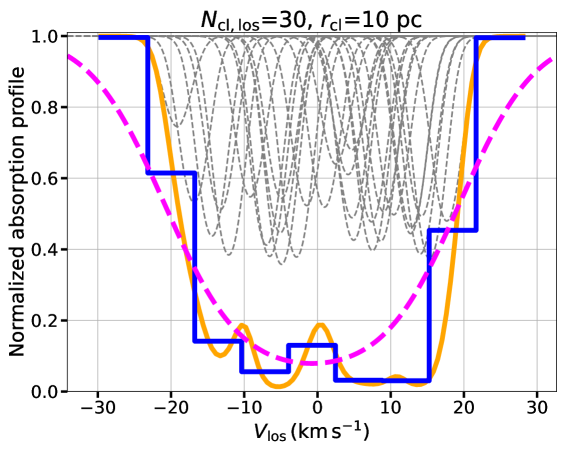
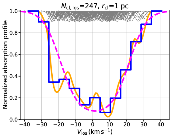
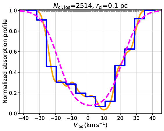
Figure 12: Normalized MgII absorption profile for various cloudlet sizes in a CC with $M_{\rm CC}=10^{7}\,M_{\odot}$ and $R_{\rm CC}=10$ kpc along a LOS passing through the center of the CC. The dashed grey lines show the individual intersected cloudlets. The orange lines show the overall absorption profiles from the intersected cloudlets along the LOS. The blue lines show the overall absorption profile smoothed with a velocity resolution of $6\,\rm km\,s^{-1}$. The dashed magenta lines show the absorption profile for the misty CC model along the sightline passing through the CC center (see section 2.1 for the definition of the mist limit and section 2.4 on how to calculate the CC absorption profile in the mist limit). As the size of cloudlets decreases from $10$ to $0.1$ pc (left to right panels) more and more cloudlets are intersected along the LOS. With an increase in the intersected cloudlets, the overall absorption profiles become broader with fewer absorbing components. For cloudlet size $\lesssim 1$ pc, our misty CC model (dashed magenta line) provides a good match to the total absorption profile.

After obtaining $b_{\rm turb}$ values for all such absorbing components along all the $10^{4}$ LOSs, we calculate the 1D turbulent velocity dispersion $\sigma_{\rm turb}$, where $\sigma_{\rm turb}=b_{\rm turb}/\sqrt{2}$. Further, we compute the mean and standard deviation of the $\sigma_{\rm turb}$ distribution (excluding $\sigma_{\rm turb}=0$ components). Figure 11 shows the ratio of the mean to standard deviation of $\sigma_{\rm turb}$ (ignoring the unblended $\sigma_{\rm turb}=0$ components) as a function of the area covering fraction ($f_{\rm A}^{\rm cl}$) for various CC sizes and a fixed cloudlet size of $5$ pc. We calculate the area covering fraction from our $10^{4}$ sightlines. For example, the number of sightlines along which at least one cloudlet is intersected is $9885$ and $9997$ for $R_{\rm CC}=30$ and $10$ kpc, respectively, implying an area covering fraction of $0.9885$ and $0.9997$.

As $R_{\rm CC}$ decreases for a fixed $r_{\rm cl}$, more lines get blended, and we get larger $\sigma_{\rm turb}$ values on average. Fig. 11 shows that when $f_{A}^{\rm cl}\approx 1$, the mean becomes larger than the standard deviation (ratio becomes larger than $1$) in the $\sigma_{\rm turb}$ distribution (excluding unblended absorption profiles with $\sigma_{\rm turb}=0$). This indicates that more blending should cause the mean to increase more rapidly than the standard deviation. If blending is not extreme (for cases not too deep into the mist limit), the distribution function of $\sigma_{\rm turb}$ (not shown) can be approximated as a power-law with $dN_{\rm abs}/d\sigma_{\rm turb}\propto\sigma_{\rm turb}^{-p}$, with the power-law index $p$ decreasing with an increasing $f_{A}^{\rm cl}$. A shallower power-law has a larger ratio of its mean to its standard deviation. This explains the increase in the ratio of the mean to standard deviation of $\sigma_{\rm turb}$ distribution with increasing (decreasing) $f_{A}^{\rm cl}$ ($R_{\rm CC}$). For extreme blending (c.f. the right panel of Fig. 12), the $\sigma_{\rm turb}$ PDF approaches a Poisson-like distribution (which itself approaches a Gaussian from the central limit theorem) with the mean increasing faster than the standard deviation. This explains the steep rise in the ratio of mean to standard deviation as $f_{A}^{\rm cl}$ approaches unity in Fig. 11.

3.1.1 Line blending with smaller cloudlets

Figure 12 shows the impact of smaller cloudlets and, therefore, a larger number of cloudlets in a CC on the overall absorption profile along a LOS. Instead of generating cloudlets throughout the entire CC ($M_{\rm CC}=10^{7}\,M_{\odot}$, $R_{\rm CC}=10$ kpc), which would yield an excessively large number of cloudlets ($\sim 10^{10}$ for $r_{\rm cl}=1$ pc), we focus on a smaller cylindrical region along the LOS to keep the total cloudlet count computationally manageable. We select a cylinder with a radius of $50$ pc and a height of $20$ kpc, positioning it at the center of the CC. This allows us to generate much fewer cloudlets in a reduced volume. We vary the size of spherical cloudlets with $r_{\rm cl}=10,1$, and $0.1$ pc and a fixed $n_{\rm cold}=10^{-2}\,\rm cm^{-3}$. We also assign turbulent velocity to each cloudlet as discussed previously. We then shoot a LOS through the center of the cylinder/CC and compute the number of intersected cloudlets, the respective column density, and the LOS velocity. With these, we generate the absorption profiles of intersected cloudlets as shown with dashed grey lines in Figure 12. The orange solid line is the overall absorption profile from all the intersected cloudlets. The blue line shows the overall absorption profile smoothed with a velocity resolution of $6$ km s^-1. The dashed magenta line shows the absorption profile from our misty CC model with $M_{\rm CC}=10^{7}\,M_{\odot}$ and $R_{\rm CC}=10$ kpc along a LOS passing through the center of CC.

As the cloudlet size decreases, more cloudlets are generated to maintain the same cold gas mass in a CC. This results in more intersected cloudlets along a LOS ($30,247$, and $2514$ cloudlets for $r_{\rm cl}=10,1$, and $0.1$ pc). The larger number of intersected cloudlets results in an overall broad absorption profile. The overall absorption profiles for $\leq 1$ pc cloudlets (middle and right panels of Fig. 12) match the absorption profile predicted by our misty CC model (dashed magenta line). We also fit Voigt profiles to the required number of components (number of components seen in orange line) and determine the best-fit column density and turbulent broadening for the individual components in all three cases. By adding the best-fit column densities for all the components, we obtain the total column densities of $\log_{10}N_{\rm MgII}=13.35,13.23$, and $13.24$ for $r_{\rm cl}=10,1$, and $0.1$ pc, respectively. Simply adding the column density of intersected cloudlets results in the same values for the respective cases. This verifies that column density is estimated very accurately by Voigt profile fitting of components, despite the extreme blending of individual cloudlet absorption profiles. The column density for the misty CC model is $\log_{10}N_{\rm MgII}=13.23$, which matches well for $r_{\rm cl}\lesssim 1$ pc. This signifies that the turbulent velocity of individual tiny cloudlets results in the turbulent broadening of the CC, well modeled by our misty CC ansatz.

4 Direct modeling of cloudlets & CCs across CGM

In Section 2, we assumed that CCs are misty and focused only on the distribution of CCs in the CGM. Rather than assuming the mist limit, in this section, we extend the work further and distribute the cold cloudlets explicitly within all the CCs across the entire CGM. We analyze the distribution of cloudlets within CCs and CCs across the CGM and check for the parameters that best match the observations. The exercise in section 3 allowed us to investigate the impact of minuscule cloudlets on the observed absorption spectrum. Because of the computational cost, such small cloudlets cannot be populated across the entire CGM. This section takes an approach similar to CloudFlex (H23) and similarly cannot reach the mist limit because of computational limitations. In fact, our approach in this section is even more expensive because the distribution functions of various observables from a single CC were combined analytically in H23, but here we also treat the CCs from first principles. The range of investigations in this work allows us to understand the relations between these various related approaches, namely, mCGM, mCC, and CloudFlex.

	Parameter	Fiducial Value	Tested Range	Description
CGM	$R_{\rm CGM}$ (kpc)	280	–	Radius of the CGM
	$M_{\rm cold}$ ($\rm M_{\odot}$)	$10^{10}$	$10^{9},5\times 10^{9},10^{10}$	Total cold gas mass in CGM
	$n_{\rm cold}$ ($\rm cm^{-2}$)	$10^{-2}$	$5\times 10^{-3},10^{-2},10^{-1}$	Number density of cold gas
cloud complex	$N_{\rm CC}$	$10^{3}$	$10^{2},10^{3},10^{4}$	Number of CCs
	$D_{\rm min}$ (kpc)	$10$	–	Minimum distance of CC from galactic center
	$D_{\rm max}$ (kpc)	$280$	–	Maximum distance of CC center from galactic center
	$\alpha$	$1.2$	$0.2,1.2,2.2$	Power-law index of radial distance of CC center
cloudlet	$d_{\rm min}$ (kpc)	$0.1$	–	Minimum distance of cloudlet from CC center
	$d_{\rm max}$ (kpc)	$10$	$5,10,20$	Maximum distance of cloudlet from CC center
	$\beta$	$0.2$	$0.2,1.2,2.2$	Power-law index of radial distance of cloudlet from CC center
	$a_{\rm min}$ (kpc)	$0.01$	$0.1,0.01$	Minimum semi-axes length of a cloudlet
	$a_{\rm max}$ (kpc)	$1$	–	Maximum semi-axes length of a cloudlet
	$\gamma$	$2.2$	$0.2,1.2,2.2$	Power-law index of semi-axes length of a cloudlet

Table 2: Model parameters, their fiducial values, tested range, and description for direct modeling of cloudlets in CCs spread throughout the CGM.

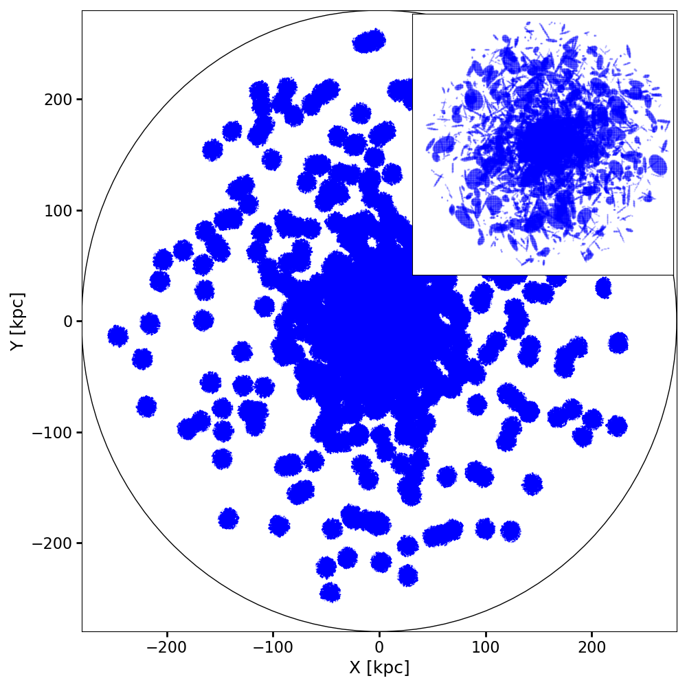
Figure 13: LOS projected distribution of ellipsoidal cloudlets in the CGM for $M_{\rm cold}=10^{10}\,\rm M_{\odot}$, $N_{\rm cc}=10^{3}$, $n_{\rm cold}=10^{-2}\,\rm cm^{-3}$, $\alpha=1.2$, $\beta=0.2$, and $\gamma=1.2$ (see Table 2 for parameter description). Each circular region shows a CC within which ellipsoidal cloudlets are present. The inset shows the cloudlet distribution in one of the CCs. Due to the power-law nature of the distribution of CCs and a larger path length through the CGM center, more CCs are found in the central region than in the outskirts. In this case, $\approx 4\times 10^{6}$ total cloudlets are generated, with $\approx 4\times 10^{3}$ cloudlets per CC. The distribution of these cloudlets shows qualitative similarity to Figure 7 of Ramesh et al. (2024) that shows a snapshot from a high-resolution simulation of a Milky Way-like CGM.

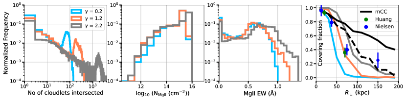
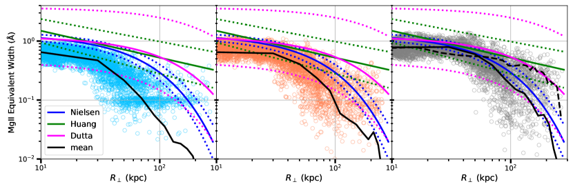
Figure 14: The three top panels show the normalized histogram of the number of intersected cloudlets, $\log_{10}N_{\rm MgII}$, and MgII EW. The top right panel shows the MgII covering fraction (for EW > $0.3\mathring{\rm A}$) as a function of the impact parameter computed in radial bins of $20$ kpc width. The solid black line showing the covering fraction from our fiducial misty CC model overpredicts the covering fraction, but the black dashed line showing the covering fraction for the power-law cold gas density profile (see section 5.3 & Fig. 16) agrees with observations. The light blue, orange, and grey colors correspond to $\gamma=0.2,1.2,2.2$, the power-law index of the semi-axes distribution of ellipsoidal cloudlets. Note that the larger the $\gamma$, the larger the number of cloudlets, keeping other parameters fixed. The total number of cloudlets generated for $\gamma=0.2,1.2,2.2$ are $\sim 10^{5},10^{6},10^{8}$, respectively. In the bottom panels, the colored scatter points show the total MgII EW along all the LOSs as a function of the impact parameter for three values of $\gamma$. The color of the points is consistent with the top panels. The black solid line in each bottom panel shows the mean EW. The dashed black line in the bottom right panel shows the mean EW for our fiducial misty CC model (see right panel of Fig. 7). The blue, green, and magenta solid lines show the best-fit relations from Nielsen et al. (2013), Huang et al. (2021), and Dutta et al. (2020) respectively. The observed EW trend matches better for increasingly misty CCs (corresponding to larger $\gamma$s) and seems to approach the average profile from our fiducial misty CC model. As expected, the misty limit is harder to achieve at large radii.

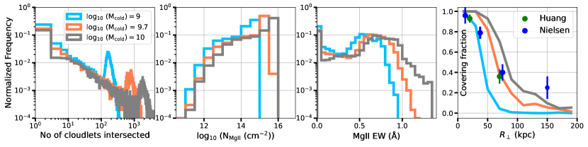
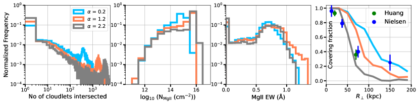
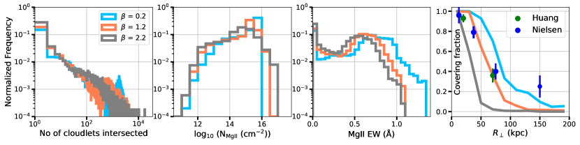
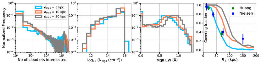
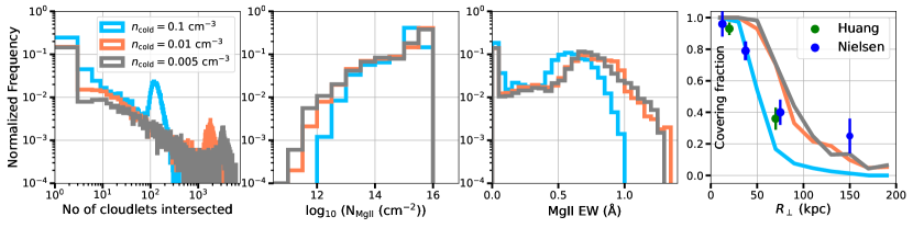
Figure 15: The three left columns show the histograms of the number of intersected cloudlets, MgII column density, and MgII EW (the same as the three top left panels in Figure 14) to show variation with different parameters. Similarly, the right panel shows the MgII covering fraction in radial bins of $20$ kpc width for MgII EW $>0.3\mathring{\rm A}$. For each row, we vary a single set of parameters and hold the other parameters fixed to their fiducial values.

Generation of CCs across the CGM: We first generate the centers of $N_{\rm CC}$ CCs with a power-law distribution in $r$ with an index $\alpha$, as done in Section 2 (see Eq. 7). To determine the 3D coordinates of the centers of each CC, we follow the procedure described in the second paragraph of section 2.4. The lower and upper limits of radial (galactocentric) distances of the centers of these CCs are $D_{\rm min}=10$ kpc and $D_{\rm max}=280$ kpc, respectively. For the fiducial case, we adopt $N_{\rm CC}=10^{3}$ and $\alpha=1.2$ (as in our fiducial mCC model), but also check the variation with $N_{\rm CC}=10^{4}$ and $\alpha=0.2,2.2$ (see Table 2).

Location of Cloudlets: After generating all the CCs, we populate cold cloudlets in each of them until the total cloudlet mass reaches the total cold gas mass $M_{\rm cold}$ (our fiducial value is $10^{10}M_{\odot}$; we cannot try a larger $M_{\rm cold}$ because of computational limitations). As in our mCC model, for simplicity, we assume the cold gas density to be constant $n_{\rm cold}$ (fiducial value $0.01$ cm^-3) throughout CGM. We use a power-law distribution of index $\beta$ for the distribution of cloudlets as a function of radial distance from the center of each CC. This is similar to what we did for distributing CCs across the CGM. The lower and upper limits of distances of the centers of cloudlets from a CC center are $d_{\rm min}$ and $d_{\rm max}$, respectively. To determine the 3D location of the centers of each cloudlet, we follow the same procedure as adopted for determining the centers of CCs in the CGM. For the fiducial case, we adopt $M_{\rm cold}=10^{10}\,\rm M_{\odot}$, $n_{\rm cold}=10^{-2}\,\rm cm^{-3}$, $\beta=0.2$, $d_{\rm max}=10$ kpc, $d_{\rm min}=0.1$ kpc. We also check the variation in observables due to variation in most of these parameters (see Table 2).

Shape and size of cloudlets: We assume the cloudlets to be ellipsoidal since they are expected to be non-spherical in general. The ellipsoidal cloudlets have three semi-axes and three rotation angles as parameters. We generate the semi-axes from a power-law distribution with index $\gamma$. The lower and upper limits of the semi-axes are $a_{\rm min}$ and $a_{\rm max}$ respectively. The three rotation angles are generated from a uniform distribution between $0$ and $2\pi$. For our fiducial case, we adopt $\gamma=2.2$, $a_{\rm min}=0.01$ kpc and we fix $a_{\rm max}=1$ kpc. We vary these parameters to check their impact on the observables (see Table 2).

We assign 3D turbulent velocity to each cloudlet following the method in the previous section to generate the turbulent velocity field in the full CGM (on a $700^{3}$ grid) and assign the velocity of each cloudlet to the nearest grid value. Table 2 lists all the parameters, their fiducial values, and the variations that we tried. We allow cloudlets to overlap as ensuring non-overlapping cloudlets is very expensive, and it has a minimal impact on the results (see section 2.2.1 in H23). The total number of cloudlets generated will depend on parameters $a_{\rm min}$, $a_{\rm max}$ and $\gamma$. Decreasing $a_{\rm min}$, $a_{\rm max}$, $n_{\rm cold}$ and increasing $\gamma$, $M_{\rm cold}$, while holding other parameters fixed, will result in more cloudlets.

Once we generate all the CCs and cloudlets, we shoot $10^{4}$ sightlines (uniformly spaced in $\log_{10}r$) into the CGM. Fig. 13 shows the LOS projected distribution of cold gas in the CGM. The circular regions show the CCs within which ellipsoidal cloudlets are distributed. There are more CCs in the central region than in the outskirts due to the power-law distribution in $r$ ($\alpha=1.2$) and due to a longer path length through the center of the CGM. The inset shows the LOS projected distribution of cloudlets in one of the CCs. Due to the ellipsoidal nature and different rotation angles, cloudlets with different shapes and sizes can be seen.

Next, we calculate the number of cloudlets intersected and intersected lengths along all the $10^{4}$ LOSs. We then calculate MgII column density using the length intersected through individual cloudlets along a sightline, assuming a conversion factor of $1.7\times 10^{-6}$ (corresponding to 1/3 solar metallicity; see Appendix A) to go from the total number density of cold gas ($n_{\rm cold}$) to MgII number density. To determine the total MgII EW along a sightline, we first generate the total absorption profile due to all the intersected cloudlets along a LOS. We then calculate the area under the total absorption profile as the total EW along a LOS. Note that simply adding EWs from individual intersected cloudlets results in a higher total EW. We assume the temperature of the cold gas to be $10^{4}$ K which corresponds to the Doppler $b$ parameter of $2.6$ km s^-1 for MgII. In this section, we do not consider turbulent broadening within a cloudlet. The turbulent broadening across the pc scale cloudlets is less than thermal broadening, so it does not significantly affect our results.

4.1 Comparing with observations

Figure 14 shows the various observable statistics with the variation in $\gamma$, the power-law index of our cloudlets’ semi-axis length distribution (size distribution). We fix the other parameters to the fiducial values (see Table 2). In the top panel, we show the normalized histogram of the number of intersected cloudlets, $\log_{10}N_{\rm MgII}$, and MgII EW. The top right panel shows the MgII covering fraction (EW > $0.3\mathring{\rm A}$, to be consistent with Nielsen et al. 2013; Huang et al. 2021) as a function of the impact parameter computed in every $20$ kpc bin. The solid black line shows the covering fraction from the misty CC model with fiducial parameters for power-law distribution. The dotted black line shows the covering fraction for the case with varying the $n_{\rm cold}$ as a function of $r$, which in turn changes the fraction of MgII accordingly (see Figure 16). The light blue, orange, and grey lines show the variation with $\gamma=0.2,1.2,2.2$, respectively. As $\gamma$ increases, the number of cloudlets also increases since the probability of generating smaller cloudlets is higher. The number of cloudlets generated for $\gamma=0.2,1.2,2.2$ is $\sim 10^{5},10^{6},10^{8}$, respectively. Due to the larger number of cloudlets, the number of intersected cloudlets is also high (top left panel). The column density distribution (top middle panel) does not show significant variation although the number of sightlines with a higher column density is higher for $\gamma=2.2$. MgII EW also increases with $\gamma$ (top right panel) as more and more cloudlets are intersected along a LOS. While the maximum column density in all three cases is $\sim 10^{16}\,\rm cm^{-2}$, there is a significant variation in the maximum EW, perhaps because at $N_{\rm MgII}\gtrsim 10^{15}$ cm² the EW starts increasing faster as compared to the flat part of the curve of growth (Fig. 5). Another reason is a larger number of kinematic components for a larger number of cloudlets along the LOS.

In the bottom panels of Fig. 14, we show the MgII EW as a function of the impact parameter for our $10^{4}$ LOSs. The scattered points are the total EW values along each LOS. The light blue (left panel), orange (middle panel), and grey (right panel) colors show the EW values for $\gamma=0.2,1.2,2.2$. The solid blue, green, and magenta line shows the best-fit relation of the observed data from Nielsen et al. (2013), Huang et al. (2021), and Dutta et al. (2020) respectively. The solid black line shows the mean EW profile in each panel. As we see from left to right in the bottom panel, the mean EW increases at all the impact parameters (faster in inner regions and slower in outer). It shows that $\gamma=2.2$ with other parameters set to their fiducial values best match the observed range. Note that the $\gamma=2.2$ model with other parameters fixed to their fiducial value generates $\approx 10^{8}$ cloudlets. The fiducial number of CCs is $10^{3}$ which means that each CC has $\approx 10^{5}$ cloudlets. This is less than the number of cloudlets $\sim 10^{7}$ generated in a single CC for mist limit in section 3. Therefore, the cloudlets are not in the completely misty limit within a CC for these fiducial parameters. It is evident that as the number of cloudlets increases (increasing $\gamma$), the observed EW is better matched with the observational range, especially at large radii. In fact, our fiducial mist CC model (shown in the bottom right panel with a black dashed line, is the closest match to the observations. To attain the mist limit within each $10^{3}$ CC, one needs to generate a total of $\sim 10^{10}$ cloudlets in the CGM, which is computationally prohibitive. Therefore, we are limited to generating $\approx 10^{8}$ cloudlets in the entire CGM, which correspond to $\sim 10^{5}$ cloudlets in each CC. So the LOSs are not in the mist limit in this section for any parameter combination mentioned in Table 2, especially at large radii with a short path length through the CGM.

In Figure 15, we show the results similar to the top panels of Figure 14 by varying cold gas mass ($M_{\rm cold}$), power-law index of distribution of CCs ($\alpha$), power-law index of distribution of cloudlets within CC ($\beta$), the size of CC ($d_{\rm max}$), and cold gas number density ($n_{\rm cold}$). While showing the variation with a parameter, we fix the other parameters to their fiducial values.

The first row in Fig. 15 shows the variation with $M_{\rm cold}=10^{9},5\times 10^{9}$, and $10^{10}\,\rm M_{\odot}$. As the cold gas mass increases, the number of cloudlets increases, leading to more intersected cloudlets along the LOS, which in turn raises the MgII column density and EW. The second row shows the variation with $\alpha$, the power-law index of the radial distribution of CCs. The number of cloudlets is the same for all the values of $\alpha$. As $\alpha$ increases, the CCs become more concentrated toward the center. This leads to a higher number of intersected cloudlets along the LOS in the central region, resulting in a larger column density. However, the EW shows different trends due to the close packing of cloudlets in the LOS velocity space, which reduces the EW compared to a more uniform spread of cloudlets in the LOS velocity. The observed covering fraction is well produced for $\alpha=1.2$ at all the impact parameters, which suggests a power-law distribution of CCs consistent with our fiducial misty CC (mCC) model from section 2.

The third row in Fig. 15 shows the variation when $\beta$, the power-law index for the distribution of cloudlets within a CC, changes. Even in this case, the number of cloudlets is the same. A larger value of $\beta$ suggests that the cloudlets are more concentrated towards the center of a CC. This results in more intersected cloudlets along a LOS passing close to the center of the CC. The column density increases with $\beta$, while EW decreases due to the close packing of cloudlets in velocity space. The covering fraction profile indicates a roughly uniform distribution of cloudlets within a CC ($\beta=0.2$) consistent with section 3. The fourth row shows the variation with $d_{\rm max}$, the CC size. For larger values, the cloudlets are more dispersed while for smaller $d_{\rm max}$, the cloudlets are tightly packed. The smaller CC results in a higher number of intersected cloudlets, and a larger column density. The EW remains roughly the same due to the similar velocity of the cloudlets in all three cases. Decreasing the CC size results in EW trends similar to that in the previous case due to the close packing of cloudlets in velocity space. The fifth row shows the variation with the cold gas number density. As the density increases, the number of cloudlets decreases as more massive cloudlets are generated. The smaller value of density results in a larger number of intersected cloudlets. The column density roughly remains constant as it takes into account the number density as well as the intersected cloudlets along a LOS. The EW increases for smaller values of number density, as the number of cloudlets generated is higher, and they are more spread out in LOS velocity. The number density of $10^{-2}\,\rm cm^{-3}$ well matches the observed covering fraction profile.

5 Discussion

Now we discuss the various implications of our models in modeling and understanding the multiphase CGM revealed by multi-wavelength observations. Our models and other similar approaches (e.g., ; , Faerman & Werk 2023) for the cold CGM go beyond the traditional hydrostatic models describing the hot CGM. The primary aim of these models is to provide robust physical insights rather than precisely matching the quasar absorption data (which are still biased by spectra quality and analysis methods).

5.1 Utility of CC-like approaches to model multiphase CGM

While an extreme idealization, CCs are useful building blocks of a multiphase CGM. Unlike the completely misty limit, CCs can give a non-unity covering fraction of cold and warm gas as probed by quasar sightlines. Moreover, the statistics of column densities and their covering fractions can constrain the mass of the cold gas, typical sizes of CCs, their numbers, and their occurrence with the distance from the center.

Most importantly, since the number of cloudlets in a CC is expected to be much larger than the number of CCs filling the CGM, it is computationally efficient to model CCs analytically in the mist limit and then populate their Monte Carlo realization to compare the post-processed column density and equivalent width statistics with observational inferences.

Our work demonstrates that the observationally inferred distribution of the inferred MgII equivalent width favors a misty CGM with several cloudlets along each LOS across a single CC (e.g., see the bottom panels of Fig. 14 which compare the model EW distribution with the observed range). This translates into a cloudlet size of $\lesssim$ few pc, which is beyond the reach of even the highest resolution galaxy formation simulations (e.g., see Ramesh et al. 2024). A small cloudlet size is also required for the CGM cold gas, in the form of cloudlets, to be suspended in long-lived CCs (see section 2.1.1); large enough cloudlets will simply precipitate towards the galactic center.

5.1.1 Comparison with D24

A large variation in EW and column density at the same distance from the galactic center implies that the misty cold gas does not fill the entire CGM uniformly. A more accurate description is in terms of misty CCs that fill the CGM sporadically. Such a model can naturally explain the large variation in column density along different sightlines (see Fig. 4).

5.1.2 Comparison with H23

H23 computes the statistical properties of CCs from first principles by populating them with cloudlets with a range of masses (assuming a power-law distribution in the cloudlet mass, $dN/dm_{\rm cl}\propto m_{\rm cl}^{-\alpha}$). For a constant density cloudlet, this corresponds to a size distribution of $dN/dr_{\rm cl}\propto r_{\rm cl}^{-3\alpha+2}$ ($r_{\rm cl}^{-4}$ for their fiducial parameters; corresponds to many more small cloudlets compared to the big ones). The mass/volume distribution of cloudlets $dV/dr_{\rm cl}\propto r_{\rm cl}^{3}dN/dr_{\rm cl}\propto r_{\rm cl}^{5-3\alpha}$; the area distribution $dA/dr_{\rm cl}\propto r_{\rm cl}^{2}dN/dr_{\rm cl}\propto r_{\rm cl}^{4-3\alpha}$. Similarly, the column density distribution $dN_{\rm cold}/dr_{\rm cl}\propto r_{\rm cl}dN/dr_{\rm cl}\propto r_{\rm cl}^{3-3\alpha}$ is dominated by the smallest cloudlets. For H23’s fiducial value of $\alpha=2$, the mass/volume, area, and column densities (even more so than mass) are all dominated by the smallest cloudlets. For power-law distributions, the average properties are typically dominated by either the higher or the lowest (as in the present case) cutoff. This justifies our misty-CC model made up of infinitesimal cloudlets (section 2) that provide a computationally inexpensive way to produce observables from just thousands of CCs that can be compared efficiently with observations.

H23 carried out a comprehensive study of the variation of various parameters of their model of cloudlets within CCs. However, they were limited by computational cost in generating an enormous number of small cloudlets for their models approaching the mist limit. They found that the cold gas mass, the smallest cloudlet mass, the cold gas density, and the CC size most affected the column density and EW distributions. The variation of other parameters within a reasonable range, such as the cloudlet size distribution, their radial distribution within CC, and turbulent velocity parameters, had a relatively minor impact. Their comprehensive exploration allows us to just focus on the complementary aspects in our work. In addition to the misty CC model (section 2), we study the observational properties of CCs populated with tiny (up to 0.1 pc) cloudlets and their implications for the realistic modeling of the multiphase CGM. In particular, we study how the cloudlets within a CC start to overlap increasingly in velocity space with a decreasing cloudlet size (section 3). This motivates our misty CC model, in which we approximate the spread in LOS velocity of numerous cloudlets with a single turbulent broadening parameter (see Fig. 12). Further, we model ellipsoidal cloudlets from first principles and populate the entire CGM with these. This approach is even more expensive than H23’s approach but produces results largely consistent with them.

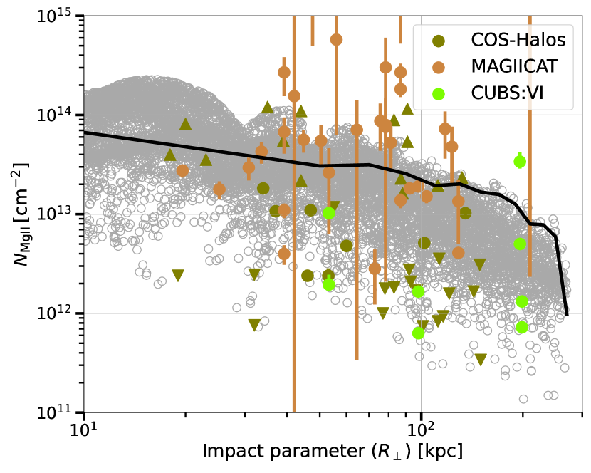
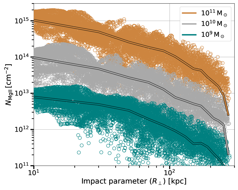
Figure 16: The top panel shows the MgII column density for the cold gas number density profile given by Eq. 18 and assuming our fiducial misty CC parameters, $M_{\rm cold}=10^{10}M_{\odot}$, $R_{\rm CC}=10$ kpc, and power-law index for radial distribution of CCs $\alpha=1.2$. Here, we use the MgII ion fraction based on the density of cold gas at a given radius, assuming photoionization equilibrium (PIE) with KS18 (Khaire & Srianand 2019) background UV radiation field (see Fig. 18). The black solid line shows the average MgII column density with a constant MgII ionization fraction of $0.33$ (see Appendix A). Note that the average column density with a constant $f_{\rm MgII}$ is reduced at the center and enhanced in the outskirts, as expected. In the bottom panel, we show the MgII column density for our fiducial mCC model and $M_{\rm cold}=10^{9},10^{10}$, and $10^{11}\,\rm M_{\odot}$ in green, grey, and orange, respectively. The solid lines with black borders in similar colors show the average column density. Again, as in Fig. 8, $M_{\rm cold}\sim 10^{10}\,\rm M_{\odot}$ explains the observed distribution better than other cold CGM mass values.

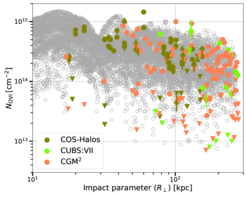
Figure 17: Column density distribution of OVI along $10^{4}$ sightlines, tracing $\sim 10^{5.5}$ K warm phase, as predicted by our fiducial CC model with a simple prescription for warm gas (see section 5.3). The cold ($10^{4}$ K) gas density profile is given by Eq. 18, and the $10^{5.5}$ K warm phase is assumed to exist in pressure equilibrium with it. Moreover, we assume OVI ion fraction from photo+collisional ionization equilibrium and assume similar cold and warm gas masses. The observed data points are from COS-Halos (Werk et al. 2013), CUBS (Qu et al. 2024), and CGM² (Tchernyshyov et al. 2022) surveys. The spread of OVI columns from our Monte Carlo model matches well with the observed spread.

5.2 Variation with cold gas number density profile

Throughout our work, we assume a constant value of cold gas density ($n_{\rm cold}=0.01$ cm^-3) across the CGM. In reality, the pressure of the cold gas is expected to be higher in the central regions than in the outskirts. This pressure variation will result in density variation across the CGM, with higher density in the central regions and lower density in the outskirts. We now check the impact of density variation on the MgII column density by assuming the cold gas density profile as

$$n_{\rm cold}(r)=0.2\times\left(\frac{r}{20\rm\,kpc}\right)^{-1.5}\,\rm cm^{-3}.$$ (18)

The CGM is expected to have a shallower density profile compared to the dark matter density because of feedback (e.g., see Fig. 2 in Sharma et al. 2012 for the hot gas density profiles inferred in groups and clusters), and we try this specific form to test the impact of varying $n_{\rm cold}$ with radius. We then populate $N_{\rm CC}=10^{3}$ CCs with $R_{\rm CC}=10$ kpc in the CGM with $M_{\rm cold}=10^{10}\,\rm M_{\odot}$. The variation in the physical density of cold gas just changes the MgII ion fraction as a function of radius (see Fig. 16).

The grey points in the top panel of Figure 16 show the MgII column density along $10^{4}$ lines of sight. These points use the density-dependent MgII ionic fraction to compute the column density (see Fig. 18). In contrast, the black line shows the average MgII column density assuming a constant MgII ion fraction. Recall that the distribution of CCs here is identical to our fiducial misty CC model, but the physical density of cold cloudlets (and hence their volume fraction within a CC) is different. Comparing the black line and grey points, it is evident that the average column density is enhanced (reduced) at the center (outskirts) of the CGM, as expected due to higher (lower) MgII ion fraction at higher (lower) cold gas density (see figure 18). We also calculate the MgII EW distribution for these sightlines (not shown) and calculate the covering fraction of sightlines with MgII EW $>0.3\mathring{A}$ using the dashed black line in the top right panel of Fig. 14, which match the observational trends.

The bottom panel of Figure 16 shows the MgII column density distribution for different cold gas masses ($10^{9},10^{10},10^{11}M_{\odot}$) in circles of different colors. The solid lines with black borders in the respective colors show the average column density in each case. Again, a cold CGM mass of $M_{\rm cold}=10^{10}\,\rm M_{\odot}$ explains the observations better than other mass values.

5.3 Modeling intermediate temperature gas

The primary focus of this paper is on modeling the cold gas. In principle, the same setup can also be applied to the intermediate temperature gas (warm gas) with few modifications. The warm gas is also expected to reside in clumpy structures like CCs but with a larger volume fraction as compared to cold gas because of its lower (physical) density. To model the warm gas, we consider the misty cold CCs in the CGM. Each cold CC is assumed to have not only cold cloudlets but also warm and hot gas inside it. The warm gas is expected to envelop the cloudlets within a CC (see Fig. 8 in Armillotta et al. 2017). The cold cloudlet volume fraction within a CC is small ($\sim 0.016$; see Eq. 10). Being 10-30 times lower density, the warm gas (traced by OVI) will occupy a larger volume by a similar factor, assuming a similar mass in warm and cold gas (a similar cold and warm gas mass is suggested by Table 3 in D24). This implies a volume fraction of the warm phase in a CC $\sim 20-50$%; the majority of volume, even within a CC, is in the hot phase. To compute the density of the OVI traced warm gas, we assume pressure equilibrium between the cold ($10^{4}$ K) and warm ($10^{5.5}$ K) phases. We assume our CCs to be misty even in the warm phase, shoot lines of sight through the CGM, and compute the column density using the photo+collisional ionization equilibrium OVI fraction at $10^{5.5}$ K and density given by pressure equilibrium with the cold gas profile given by Eq. 18.

Figure 17 shows the column density distribution of OVI tracing the warm ($10^{5.5}$ K) gas. The observational data points are from various surveys; COS-halos, CUBS, and CGM² (Werk et al. 2013; Qu et al. 2024; Tchernyshyov et al. 2022). Predictions from our simple misty CC model agree well with the observed distribution of OVI column density, including the upper and lower limits. This simple exercise shows the predicting power, flexibility, and computational efficiency of our misty CC model for studying the multiphase CGM. Just as the combination of the covering fraction and the average column density provides an unbiased estimate of the cold CGM mass, the same observables for OVI can be applied easily to estimate the warm CGM mass.

5.4 Astrophysical Implications

The majority of the baryonic mass in the universe is in the diffuse intergalactic and circumgalactic medium. While the IGM dominates the global baryonic mass budget of the local Universe, even within galactic halos, the majority of baryons reside in the diffuse CGM and not in the dense interstellar medium and stars. Being major matter reservoirs, the CGM controls star formation in galaxies across cosmological timescales.

Fundamental questions in CGM research are regarding the fraction of baryons in the CGM as a function of halos mass, its spatial extent, and the distribution of the CGM mass across different temperature phases. While direct observations of the volume-filling hot CGM are rare (being volume-filling and close to hydrostatic, the hot CGM is easier to model), the cold and warm phases are routinely probed through quasar absorption lines. However, since cold and warm CGM phases are not volume-filling and occur in the form of clouds, the inferred column densities show a large scatter even in a uniform galaxy sample, which prevents us from drawing robust conclusions about their mass budget.

We show that a large variation in the column density of the cold/warm ions is natural in a CGM in which these phases are not spread uniformly throughout the CGM, but are instead confined to thousands of $\sim 10$ kpc CCs spread sporadically throughout the CGM (see Figs. 4, 16, & 17). Moreover, the average column density and the area covering fraction in a uniform galaxy+quasar sample can constrain the mass of the cold and warm phases of the CGM, as illustrated in Fig. 9.

5.4.1 Inferring cold CGM mass from quasar absorption

One of the ultimate goals of our (and similar) models is to obtain a robust estimate of the cold/warm CGM mass from observations. Fig. 9 shows that a combination of the area-averaged MgII column density and the area covering fraction provides a robust proxy for the mass in cold CGM. Both ion column density and covering fraction can be inferred from observational samples of Milky Way-like galaxies probed by quasar sightlines. However, the primary observable in these studies is the transmitted flux spectrum, which at high resolution can have many components separated by small centroid velocity shifts for the same sightline. Each of these resolved components (depending on the spectral resolution of the spectrograph) can be modeled as a misty and turbulent CC along the LOS, each composed of numerous cloudlets. Physically distinct CCs may coincide in velocity space, and similarly, cloudlets within a CC may be distinct in velocity (e.g., Fig. 10). Since the column density essentially counts all the ions along the LOS, this complication does not affect the cold CGM mass estimate.

There are different approaches to analyzing absorption spectra. The most reliable technique with high spectral resolution ($\lesssim 10$ km s^-1) is to fit the absorption profile with a number of absorption components with Voigt profiles. The best fit Voigt profile can give us the turbulent broadening parameter $b_{\rm turb}$ (particularly in the presence of multiple ions tracing the same phase that coincide kinematically) and column density for each component. We can add the column densities of all components along the LOS to obtain the total column density along it. For low-resolution spectra, the Voigt profile fitting of components fails, and most studies employ the AOD (apparent optical depth) method (Savage & Sembach 1991). Under this, we obtain the optical depth spectrum and convert it into a column density spectrum (assuming that the absorption lines are not saturated). The column density spectrum is integrated to give the total ion column along the LOS. This popular method may underestimate the column density because of saturation and unresolved sub-structure. Section 3.1.1 shows that both Voigt profile fitting and even fitting a single turbulent broadened misty CC model (implying that AOD method will also work well; large cloudlets without much internal turbulence can become saturated, reducing the accuracy of the AOD/mCC method) give a good estimate of the true column density of cloudlets along a LOS even with extreme blending in LOS velocity due to thousands of cloudlets along the LOS.

Fig. 9 that plots the covering fraction versus the average column density shows that a combination of these two observables provides a good estimate of the cold CGM mass. The column density along different sightlines can give us the average column density that should be plotted on the y-axis of Fig. 9. All spectrographs have a finite sensitivity and will inevitably miss out on weak absorption components, giving us an upper limit on the LOS column density. Similarly, saturated lines can give us a lower limit on the column density (e.g., see COS-Halos markers in Fig. 3). We calculate the covering fraction on the x-axis of Fig. 9 as the fraction of LOSs with EW larger than a small enough value (say $0.1$ Å) so that the bulk of the EW distribution is sampled by observations (e.g., see Fig. 7). If these conditions are satisfied, Fig. 9 provides a robust way to estimate the cold gas mass in the diffuse CGM.

5.4.2 Quasar absorption lines versus other CGM probes

Emission is weighted toward the highest density in the CGM, so it cannot typically probe the diffuse outer CGM (except through stacking; e.g., Zhang et al. 2019), which holds most of the CGM mass (e.g., Nielsen et al. 2024). Thus, emission gives a biased estimate of the CGM mass. FRBs are sensitive to the total number of electrons along the LOS, including the contribution of IGM, FRB host galaxy, and the Milky Way (e.g., Macquart et al. 2020; Connor et al. 2024) and the CGM contribution is typically subdominant. Moreover, while FRBs may be an unbiased probe of total CGM mass, one cannot separate the contribution from different temperature phases.

Similarly, the thermal Sunyaev-Zeldovich (tSZ) effect probes the integrated pressure along the LOS and cannot distinguish between different CGM phases like FRBs. Moreover, the signal is too small to be detected in individual galaxies and requires stacking of similar mass galaxies (e.g., Bregman et al. 2022). The kinetic SZ signal is proportional to the product of the LOS velocity of the galaxy halo (determining which requires large galaxy surveys) and the electron column density, but stacking is necessary to detect the signal averaged over the whole CGM (e.g., see Schaan et al. 2021).

Therefore, quasar absorption line studies are the only means to study the various phases of the CGM. With an increasingly large number of background quasar-galaxy pairs, improving spatial and spectral resolution, and availability of a range of ions tracing a range of temperatures, quasar absorption lines have a unique position as the probe of the multiphase CGM. However, the modeling of the cold/warm phase is nontrivial, and more accurate models, going beyond the models presented in this work, are necessary to derive unbiased physical properties from observations.

Carefully combining the results from different observational probes from the CGM while being mindful of biases inherent in different techniques is the best way of obtaining robust physical constraints on the physical properties of the CGM. For this, we need robust phenomenological models of the multiphase CGM which can make testable predictions. While simulations of the CGM are steadily increasing in resolution and the included physics (Ramesh et al. 2024), we are still some way off from getting robust predictions from them because of insufficient spatial/mass resolution (we need a resolution better than a few pc in the cold phase to obtain converged results for MgII EW distribution; e.g., see section 3.1.1 & Fig. 14) and because of ambiguities related to feedback and sub-grid physics. The gap between expensive cosmological simulations and high resolution observations can be filled by novel phenomenological models such as ours.

5.5 Caveats & future directions

The observational distribution of EWs and column densities of cold and warm ion tracers in the CGM suggests a patchy distribution of cold gas in cloud complexes rather than uniformly throughout the CGM, as assumed in D24. However, our assumption of spherical CCs with a constant cloudlet size, a uniform distribution of cloudlets within a CC, a fixed turbulent broadening across a CC across all sightlines, etc. are extreme idealizations which must be tested in future. However, consistent distribution of EW distribution with a range of CC models (e.g., see Fig. 14) that matches with observations suggests that even our simple and computationally tractable misty CC model is quite accurate. We assumed spherical CCs, but they are very likely to have a head-tail structure. Moreover, with a range of cloudlets, the large ones may not be dragged enough (e.g., see Eq. 1) to remain in a turbulent CC but can instead precipitate towards the center replenishing the ISM, as required by the star formation histories over cosmological timescales (e.g., see Bera et al. 2023).

Our misty CC model can easily include a radial density profile within a CC for different phases. Moreover, similar to D24, which populate the whole CGM with a log-normal temperature (or 2-D density temperature) distribution, we can easily extend our mist CCs to have a range of temperatures and densities (which can also be adjusted according to the ambient pressure profile). These temperature and density distributions and the multiphase turbulence properties of CCs can be calibrated with detailed simulations of multiphase CGM patches (e.g., Mohapatra et al. 2022a). These models can also accommodate warm/cold gas within CCs that is mainly supported by nonthermal pressure of cosmic rays or magnetic fields, as suggested by some simulations (e.g., Sharma et al. 2010; Nelson et al. 2020; Butsky et al. 2020). The biggest advantage of the mCC model presented in section 2 is their much lower computational cost relative to models that model the cloudlets from first principles (e.g., H23, our models in section 4).

Misty CCs may also provide a useful recipe for modeling unresolved multiphase gas phenomenologically in galaxy simulations that typically lack sufficient resolution to resolve realistic CGM cloudlets (e.g., see Weinberger & Hernquist 2023; Butsky et al. 2024 for recent works along these lines). We can populate CCs aware of their origins in different parts of the CGM, such as the high-pressure galactic outflows, low-metallicity IGM filaments, galactic fountains, and high-velocity clouds, etc., and produce observables to match more sophisticated observational samples that test anisotropy of CGM absorbers relative to the galaxy’s minor axis and distance from the galactic center. The low computational cost, realism, and flexibility of our mCC model allow us to adapt it to produce observable distributions for a range of model variations.

6 Summary

Here we provide a summary of the salient aspects of this paper.

1. We present the misty cloud-complex (mCC) model to match the observed distribution of column densities and equivalent widths (EWs) of cold ions such as MgII (Fig. 16) and warm ions like OVI (Fig. 17). This model further expands and explores the connections between the misty CGM models of Dutta et al. (2024) and the Cloudflex presented by Hummels et al. (2023). The former model assumes that the cold/warm gas is uniformly spread throughout the CGM, producing a smooth variation of cold gas column density. The CloudFlex model assumes the CGM cold gas to be spread across CGM cloud complexes (CCs) and quantifies the distribution of column densities, equivalent widths across sightlines through these CCs which are populated by $\sim 10^{6}$ cloudlets (it is computationally difficult to increase the number of cloudlets beyond this). Like CloudFlex, our misty CC (mCC) model also assumes the cold gas to be spread over CCs but models the cold cloudlets analytically in the mist limit (analogous to D24). This makes our model analytically tractable and computationally inexpensive compared to CloudFlex (which has a hard time reaching the mist limit due to computational limitations). Moreover, mCC needs to populate only a thousand CCs over the CGM and can satisfactorily reproduce the observational spread of MgII EWs and other observables (e.g., see Figs. 3 & 4).

2. We demonstrate that the combination of the average CGM column density and covering fraction provides a robust estimate of the cold CGM mass (see Fig. 9). The observed distribution of the inferred MgII column density suggests a cold CGM mass $\sim 10^{10}M_{\odot}$ for Milky Way-like galaxies (see Fig. 8). Further, about $\sim 10^{3}$ CCs each of $\sim 10$ kpc seems to well match the observed distribution of MgII column density. We also find that both the component fitting and apparent optical depth (AOD) method applied to the absorption spectra provide a reasonable estimate of the column density along the sightline. The spread of LOS velocity also matches the turbulent mCC estimate based on the Kolmogorov scaling of turbulent velocity with the size of the CC.

3. We quantify the ’mist’ limit for the parameters quantifying a CC: the volume fraction of cold gas within CC $f_{V}$, the number of cloudlets $N_{\rm cl}$, and the size of CC ($L$). We find that the mist limit, for which a typical sightline encounters at least one cloudlet is reached if $N_{\rm cl}\gtrsim f_{V}^{-2}$ (see Fig. 3). Further, from the statistics of the observed absorption components, specifically the ratio of the mean turbulent broadening parameter and its standard deviation, we can infer whether the CC is in the mist limit. This ratio exceeds unity in the misty limit when there are multiple absorbing cloudlets along the LOS that produce blended absorption profiles with a larger turbulent broadening of the components (see Fig. 11). Further, we show that $\sim$ pc scale cloudlets within CCs produce extreme blending in absorption spectra, but the total absorption spectrum requires only a few components that can be well fit by the mCC ansatz of the scaling of turbulent broadening with the CC size (see Fig. 12).

4. In section 4, we directly generate cloudlets in all CCs spread throughout the CGM. We confirm that it is computationally challenging to approach the mist limit for a small number ($\lesssim 10^{6}$) of cloudlets within a CC because of numerous empty sightlines, especially for LOSs at large radii with a small number of intersected CCs (see Fig. 14). The MgII EW distribution from our direct model with smallest (and most numerous) cloudlets with a cold CGM mass of $10^{10}M_{\odot}$ matches well the distribution from our fiducial misty CC model (except at largest radii; see bottom-right panel of Fig. 14), which itself compares well with the observed EW range.

5. Finally, we demonstrate the versatility of our mCC model by assuming a realistic power-law cold gas density profile, which produces an even better match with observations (Fig. 16). Using a simple extension of our fiducial mCC model, we are also able to produce a quantitative match with the observed OVI (a tracer of warm $10^{5.5}$ K gas) column density distribution.

7 Acknowledgements

We thank Jasjeet Singh Bagla, Rajeshwari Dutta, and Cameron Hummels for the useful discussions. This work was performed in part at Aspen Center for Physics (ACP), which is supported by National Science Foundation grant PHY-2210452 and a grant from the Simons Foundation (1161654, Troyer). PS and AD acknowledge the lively discussions at ACP (in particular with Yakov Faerman and Cameron Hummels) that shaped some of the key ideas presented in this paper. Research of AD was supported by the Prime Minister’s Research Fellowship (PMRF) from the Ministry of Education (MoE), Govt. of India.

8 Data Availability

We have made all the codes and data used in this paper publicin the GitHub repo mCC.. Any other data associated with this article are available to the corresponding author upon reasonable request.

Appendix A MgII ion fraction estimates

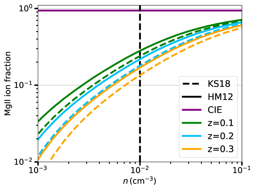
Figure 18: MgII ion fraction as a function of total number density at $10^{4}$ K. The purple line shows the MgII fraction for the Collisional Ionization Equilibrium while the green, blue, and orange colors show the values for Photoionization Equilibrium at the redshift of $0.1$, $0.2$, and $0.3$, respectively. The solid and dashed colored line shows the ion fraction with the HM12 (Haardt & Madau 2012) and KS18 (Khaire & Srianand 2019) background radiation field. The vertical dashed black line shows the number density of $10^{-2}\,\rm cm^{-3}$, the fiducial value used in our models. We have computed the ion fraction values using the radiative transfer code CLOUDY (Ferland et al. 2017). MgII ion fraction values vary from $\approx 0.1\hbox{--}0.3$ for $n=10^{-2}\,\rm cm^{-3}$ and $z\leq 0.3$. We adopt $0.33$ as the MgII ion fraction for our analysis.

The number density of MgII is given by

$$n_{\rm MgII}=\mu X\left(\frac{Z}{Z_{\odot}}\right)\left(\frac{n_{\rm Mg}}{n_{\rm H}}\right)_{\odot}\left(\frac{n_{\rm MgII}}{n_{\rm Mg}}\right)n_{\rm cold},$$ (19)

where $X=0.74$ (Asplund et al. 2009) is the hydrogen mass fraction, $\mu=0.6$ is the mean molecular weight, $Z=0.3Z_{\odot}$ (Prochaska et al. 2017) is the metallicity of the gas, $(n_{\rm Mg}/n_{\rm H})_{\odot}=3.47\times 10^{-5}$ (Ferland et al. 2017; Holweger 2001) is the solar abundance of Mg, and ($n_{\rm MgII}/n_{\rm Mg}$) is the fraction of MgII in Mg. Figure 18 shows the MgII ion fraction as a function of the total number density. The purple line shows the ion fraction in Collisional Ionization Equilibrium (CIE). The green, blue, and orange lines show the ion fraction at three different redshifts in Photoionization Equilibrium (PIE). The vertical dashed black line corresponds to the fiducial value of cold gas number density. The ion fraction varies from $\approx 0.03\hbox{--}0.9$ and we adopt $0.33$. Therefore, the conversion factor from the total number density of cold gas to MgII number density is $1.7\times 10^{-6}$.

Appendix B Standard deviation estimates

Just as we can calculate the average number of CCs along a LOS and the average path length along a CC, we can also calculate the standard deviation of these quantities.

For average CC density, which is only a function of the distance $r$ and independent of $\theta$ and $\phi$, the distribution of CCs in a radial shell is expected to be Poisson, with the variance equal to the mean number of clouds. For the number of CCs encountered along a LOS, this means that the variance in the number of CCs along a LOS equals the average number of CCs. Thus, the standard deviation in the number of CCs along a LOS is simply the square root of the average number of clouds encountered.

The deviation in the length along a single CC is given by $\sigma_{L}=\sqrt{\langle L^{2}\rangle-\langle L\rangle^{2}}$, with

$$\langle L^{2}\rangle=\frac{\int_{0}^{R_{\rm CC}}2\pi bdb\,4(R_{\rm CC}^{2}-b^{2})}{\int_{0}^{R_{\rm CC}}2\pi bdb}=2R_{\rm CC}^{2}.$$ (20)

Combining this, and Eq. 5 gives, $\sigma_{L}=\sqrt{2}R_{\rm CC}/3$.

Both the number of clouds encountered along a LOS and the path length through a CC are random variables. Thus, the variation in column density along a LOS will have contributions due to both these random variables. Adding all the deviations in quadrature (and assuming $N_{\rm CC,LOS}$ and $L$ to be independent random variables), we can write

$$\sigma_{N}^{2}=\sigma_{N_{\rm CC,LOS}}^{2}\langle L\rangle^{2}+\langle N_{\rm CC,LOS}\rangle^{2}\sigma_{L}^{2}+\sigma_{N_{\rm CC,LOS}}^{2}\sigma_{L}^{2}.$$ (21)

Here, the column density $N=\sum(n_{\rm ion})_{j}L_{j}=N_{\rm CC,LOS}Ln_{\rm ion}$ is a sum over CCs along the LOS. Recall that $\langle N\rangle=\langle N_{\rm CC,LOS}\rangle\langle L\rangle\langle n_{\rm ion}\rangle$, $\sigma_{N_{\rm CC,LOS}}/\langle N_{\rm CC,LOS}\rangle=1/\sqrt{\langle N_{\rm CC,LOS}\rangle}$ and $\sigma_{L}/\langle L\rangle=\sqrt{2}/4$. These estimates are used to show (using dotted lines) the expected deviation from average column density in Fig. 3.

References

- Afruni et al. (2019) Afruni A., Fraternali F., Pezzulli G., 2019, A&A, 625, A11
- Armillotta et al. (2017) Armillotta L., Fraternali F., Werk J. K., Prochaska J. X., Marinacci F., 2017, MNRAS, 470, 114
- Asplund et al. (2009) Asplund M., Grevesse N., Sauval A. J., Scott P., 2009, ARA&A, 47, 481
- Augustin et al. (2021) Augustin R., Péroux C., Hamanowicz A., Kulkarni V., Rahmani H., Zanella A., 2021, MNRAS, 505, 6195
- Bera et al. (2023) Bera A., Kanekar N., Chengalur J. N., Bagla J. S., 2023, ApJ, 956, L15
- Bregman et al. (2022) Bregman J. N., Hodges-Kluck E., Qu Z., Pratt C., Li J.-T., Yun Y., 2022, ApJ, 928, 14
- Burchett et al. (2021) Burchett J. N., Rubin K. H. R., Prochaska J. X., Coil A. L., Vaught R. R., Hennawi J. F., 2021, ApJ, 909, 151
- Butsky et al. (2020) Butsky I. S., Fielding D. B., Hayward C. C., Hummels C. B., Quinn T. R., Werk J. K., 2020, ApJ, 903, 77
- Butsky et al. (2024) Butsky I. S., Hummels C. B., Hopkins P. F., Quinn T. R., Werk J. K., 2024, MNRAS, 535, 1672
- Chen et al. (2023) Chen H.-W., et al., 2023, ApJ, 955, L25
- Chen et al. (2024) Chen Z., et al., 2024, arXiv e-prints, p. arXiv:2411.08485
- Connor et al. (2024) Connor L., et al., 2024, arXiv e-prints, p. arXiv:2409.16952
- Cook et al. (2023) Cook A. M., et al., 2023, ApJ, 946, 58
- Decataldo et al. (2024) Decataldo D., Shen S., Mayer L., Baumschlager B., Madau P., 2024, A&A, 685, A8
- Donahue & Voit (2022) Donahue M., Voit G. M., 2022, Phys. Rep., 973, 1
- Draine (2011) Draine B. T., 2011, Physics of the Interstellar and Intergalactic Medium. Princeton University Press
- Dutta et al. (2020) Dutta R., et al., 2020, MNRAS, 499, 5022
- Dutta et al. (2024) Dutta A., Bisht M. S., Sharma P., Ghosh R., Roy M., Nath B. B., 2024, MNRAS, 531, 5117
- Faerman & Werk (2023) Faerman Y., Werk J. K., 2023, ApJ, 956, 92
- Faucher-Giguère & Oh (2023) Faucher-Giguère C.-A., Oh S. P., 2023, ARA&A, 61, 131
- Ferland et al. (2017) Ferland G. J., et al., 2017, Rev. Mex. Astron. Astrofis., 53, 385
- Haardt & Madau (2012) Haardt F., Madau P., 2012, ApJ, 746, 125
- Hitomi Collaboration et al. (2016) Hitomi Collaboration et al., 2016, Nature, 535, 117
- Holweger (2001) Holweger H., 2001, in Wimmer-Schweingruber R. F., ed., American Institute of Physics Conference Series Vol. 598, Joint SOHO/ACE workshop “Solar and Galactic Composition”. AIP, pp 23–30 (arXiv:astro-ph/0107426), doi:10.1063/1.1433974
- Huang et al. (2021) Huang Y.-H., Chen H.-W., Shectman S. A., Johnson S. D., Zahedy F. S., Helsby J. E., Gauthier J.-R., Thompson I. B., 2021, MNRAS, 502, 4743
- Hummels et al. (2023) Hummels C. B., Rubin K. H. R., Schneider E. E., Fielding D. B., 2023, arXiv e-prints, p. arXiv:2311.05691
- Khaire & Srianand (2019) Khaire V., Srianand R., 2019, MNRAS, 484, 4174
- Licquia & Newman (2015) Licquia T. C., Newman J. A., 2015, ApJ, 806, 96
- Macquart et al. (2020) Macquart J. P., et al., 2020, Nature, 581, 391
- McCourt et al. (2012) McCourt M., Sharma P., Quataert E., Parrish I. J., 2012, MNRAS, 419, 3319
- Mihalas (1978) Mihalas D., 1978, Stellar atmospheres. W.H.Freeman & Co Ltd
- Mohapatra et al. (2022a) Mohapatra R., Jetti M., Sharma P., Federrath C., 2022a, MNRAS, 510, 2327
- Mohapatra et al. (2022b) Mohapatra R., Jetti M., Sharma P., Federrath C., 2022b, MNRAS, 510, 3778
- Nelson et al. (2020) Nelson D., et al., 2020, MNRAS, 498, 2391
- Nelson et al. (2021) Nelson D., Byrohl C., Peroux C., Rubin K. H. R., Burchett J. N., 2021, MNRAS, 507, 4445
- Nielsen et al. (2013) Nielsen N. M., Churchill C. W., Kacprzak G. G., 2013, ApJ, 776, 115
- Nielsen et al. (2016) Nielsen N. M., Churchill C. W., Kacprzak G. G., Murphy M. T., Evans J. L., 2016, ApJ, 818, 171
- Nielsen et al. (2024) Nielsen N. M., Fisher D. B., Kacprzak G. G., Chisholm J., Martin D. C., Reichardt Chu B., Sandstrom K. M., Rickards Vaught R. J., 2024, Nature Astronomy
- Pessa et al. (2024) Pessa I., et al., 2024, arXiv e-prints, p. arXiv:2408.16067
- Prochaska & Zheng (2019) Prochaska J. X., Zheng Y., 2019, MNRAS, 485, 648
- Prochaska et al. (2017) Prochaska J. X., et al., 2017, ApJ, 837, 169
- Qu et al. (2023) Qu Z., et al., 2023, MNRAS, 524, 512
- Qu et al. (2024) Qu Z., et al., 2024, ApJ, 968, 8
- Ramesh et al. (2024) Ramesh R., Nelson D., Fielding D., Brüggen M., 2024, arXiv e-prints, p. arXiv:2407.00172
- Roy et al. (2024) Roy M., Su K.-Y., Tonnesen S., Fielding D. B., Faucher-Giguère C.-A., 2024, MNRAS, 527, 265
- Rubin et al. (2012) Rubin K. H. R., Prochaska J. X., Koo D. C., Phillips A. C., 2012, ApJ, 747, L26
- Sameer et al. (2024) Sameer et al., 2024, MNRAS, 530, 3827
- Savage & Sembach (1991) Savage B. D., Sembach K. R., 1991, ApJ, 379, 245
- Schaan et al. (2021) Schaan E., et al., 2021, Phys. Rev. D, 103, 063513
- Schmidt et al. (2021) Schmidt W., Schmidt J. P., Grete P., 2021, A&A, 654, A115
- Sharma et al. (2010) Sharma P., Parrish I. J., Quataert E., 2010, ApJ, 720, 652
- Sharma et al. (2012) Sharma P., McCourt M., Parrish I. J., Quataert E., 2012, MNRAS, 427, 1219
- Srianand & Khare (1993) Srianand R., Khare P., 1993, ApJ, 413, 486
- Tchernyshyov et al. (2022) Tchernyshyov K., et al., 2022, ApJ, 927, 147
- Tumlinson et al. (2011) Tumlinson J., et al., 2011, Science, 334, 948
- Tumlinson et al. (2017) Tumlinson J., Peeples M. S., Werk J. K., 2017, ARA&A, 55, 389
- Voit et al. (2017) Voit G. M., Meece G., Li Y., O’Shea B. W., Bryan G. L., Donahue M., 2017, ApJ, 845, 80
- Weinberger & Hernquist (2023) Weinberger R., Hernquist L., 2023, MNRAS, 519, 3011
- Werk et al. (2013) Werk J. K., Prochaska J. X., Thom C., Tumlinson J., Tripp T. M., O’Meara J. M., Peeples M. S., 2013, ApJS, 204, 17
- Wu et al. (2024) Wu X., et al., 2024, arXiv e-prints, p. arXiv:2407.17809
- Zhang et al. (2019) Zhang H., Zaritsky D., Behroozi P., Werk J., 2019, ApJ, 880, 28