X-MeshGraphNet: Scalable Multi-Scale Graph Neural Networks for Physics Simulation

Abstract

Graph Neural Networks (GNNs) have gained significant traction for simulating complex physical systems, with models like MeshGraphNet demonstrating strong performance on unstructured simulation meshes. However, these models face several limitations, including scalability issues, requirement for meshing at inference, and challenges in handling long-range interactions. In this work, we introduce X-MeshGraphNet, a scalable, multi-scale extension of MeshGraphNet designed to address these challenges.

X-MeshGraphNet overcomes the scalability bottleneck by partitioning large graphs and incorporating halo regions that enable seamless message passing across partitions. This, combined with gradient aggregation, ensures that training across partitions is equivalent to processing the entire graph at once. To remove the dependency on simulation meshes, X-MeshGraphNet constructs custom graphs directly from CAD files by generating uniform point clouds on the surface or volume of the object and connecting k-nearest neighbors. Additionally, our model builds multi-scale graphs by iteratively combining coarse and fine-resolution point clouds, where each level refines the previous, allowing for efficient long-range interactions.

Our experiments demonstrate that X-MeshGraphNet maintains the predictive accuracy of full-graph GNNs while significantly improving scalability and flexibility. This approach eliminates the need for time-consuming mesh generation at inference, offering a practical solution for real-time simulation across a wide range of applications. The code for reproducing the results presented in this paper is available through NVIDIA Modulus: github.com/NVIDIA/modulus/tree/main/examples/cfd/xaeronet.

I Introduction

Numerical methods, such as finite element analysis (FEA) and computational fluid dynamics (CFD), offer high-fidelity simulations but come at a significant computational cost. With the growing demand for faster and more efficient simulations—particularly for real-time applications and design optimization—machine learning-based surrogate models have emerged as a promising alternative. Among these, Graph Neural Networks (GNNs) have garnered attention due to their natural ability to model interactions between components of structured data, such as the meshes commonly used in physical simulations.

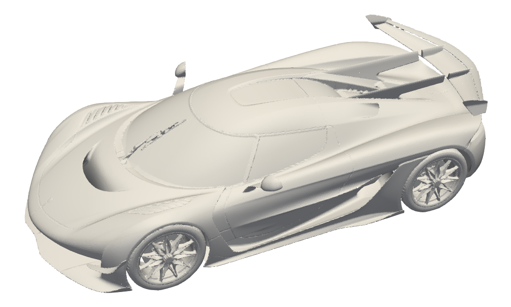
(a) Original mesh graph.

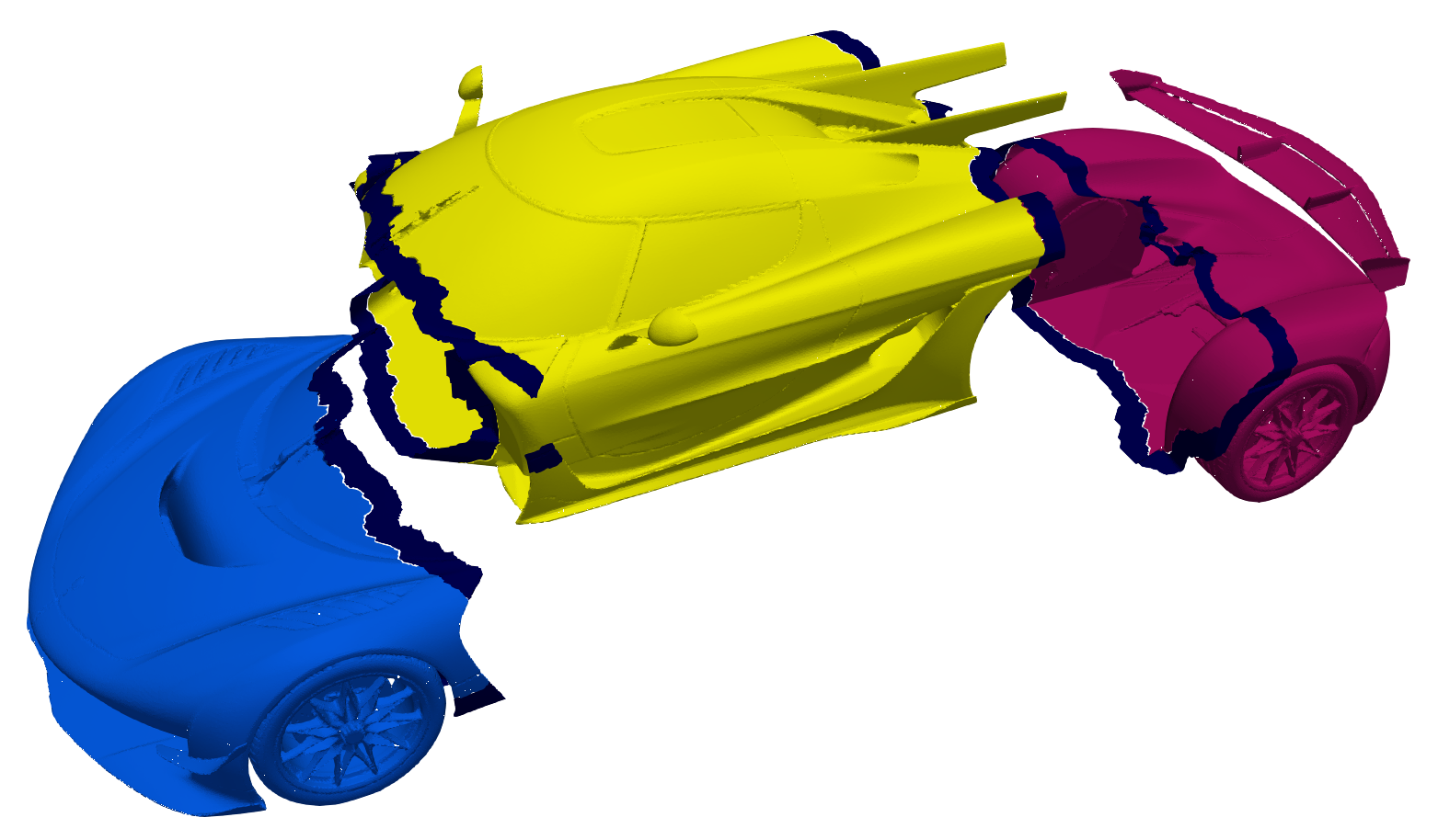
(b) Partitioned mesh graph with Halo.

Figure 1: Illustration of the partitioning scheme with Halo on a Koenigsegg car.

In recent years, several GNN models have been proposed as surrogate models for engineering simulations, particularly for systems governed by partial differential equations (PDEs). These models aim to approximate the behavior of complex systems more efficiently than traditional numerical solvers, offering faster inference times while maintaining reasonable accuracy. Early works in this field, such as GraphNet [1] and Gated Graph Neural Networks (GGNNs) [2] , have been applied to a wide range of tasks, including fluid dynamics and structural mechanics, where they model physical interactions through message passing between nodes representing simulation elements. More recent models, such as MeshGraphNet [3] and DeepMind’s Learning to Simulate framework [4], leverage mesh-based GNNs to represent structured data, where vertices represent simulation nodes and edges represent physical relationships. These models have demonstrated success in tasks such as airflow prediction and elastic deformations.

While these GNN-based models show significant promise as surrogates for complex simulations, they still face challenges related to scalability, dependence on simulation meshes, and handling long-range interactions that our proposed X-MeshGraphNet directly addresses.

Scalability: GNN models, including MeshGraphNet, struggle with large-scale simulations due to the high memory overhead associated with processing dense meshes or graphs. As the size of the mesh increases, both the computational and memory demands grow exponentially, limiting their applicability to high-resolution domains.

Dependence on Simulation Meshes: The reliance on pre-generated simulation meshes during inference presents a significant bottleneck. Generating high-quality meshes for complex geometries is time-consuming and computationally expensive, which undermines the speed advantage of surrogate models.

Multi-Scale Simulations: In multi-scale simulations, different levels of fidelity are required to capture both global and local dynamics. While multi-scale versions of MeshGraphNet have been proposed, they often require handling multiple meshes at various resolutions, which introduces additional complexity and limits usability. Moreover, downsampling and upsampling layers introduce additional memory overhead.

Topological Biases: Meshes inherently impose topological constraints that may not align with the true physical interactions of the system being modeled. This can introduce biases into the model, reducing its ability to generalize across different geometries and simulation conditions.

To address these limitations, we propose X-MeshGraphNet, a scalable, multi-scale extension of MeshGraphNet that overcomes the dependency on simulation meshes and improves scalability for large-scale simulations. Our model builds on three key innovations:

Custom Graph Construction: Instead of relying on pre-existing simulation meshes, X-MeshGraphNet generates custom graphs directly from CAD files. This is done by creating a uniform point cloud on the surface or volume of the object and connecting the k-nearest neighbor points, eliminating the need for costly meshing processes during inference.

Graph Partitioning with Gradient Aggregation: To handle large-scale simulations, X-MeshGraphNet partitions the graph into smaller subgraphs, with halo regions allowing message passing between partitions. Gradients from each partition are aggregated before model updates, ensuring that training remains equivalent to processing the entire graph at once, while maintaining computational efficiency.

Multi-Scale Graph Generation: X-MeshGraphNet introduces a multi-scale graph generation process where coarse point clouds are refined iteratively to create finer-scale point clouds, with each level being a superset of the previous. This hierarchical approach allows the model to capture global and local interactions efficiently.

In the following sections, we detail the architecture of X-MeshGraphNet and its application to large-scale physical simulations.

II Technical Overview: MeshGraphNet

MeshGraphNet is a graph-based neural network model designed to simulate physical systems by representing the mesh structure as a graph. The key idea is to use message passing between nodes in a graph to propagate information about physical states, such as velocity, pressure, or temperature, over time. The message-passing paradigm enables MeshGraphNet to capture both local and global interactions in a system governed by PDEs.

II-A Graph Representation of a Mesh

In MeshGraphNet, a mesh is treated as a graph $G=(V,E)$, where:

• $V$ is the set of nodes, corresponding to the mesh vertices,

• $E$ is the set of edges, corresponding to the connections between adjacent vertices.

Each node $i\in V$ has a feature vector $h_{i}\in\mathbb{R}^{d}$, which stores relevant physical quantities (e.g., velocity, pressure, position). Each edge $(i,j)\in E$ has a feature vector $e_{ij}\in\mathbb{R}^{k}$, which encodes information about the relationship between nodes $i$ and $j$, such as distance or relative positions.

II-B Message Passing Mechanism

The central concept of MeshGraphNet is message passing, which allows the model to iteratively propagate information between neighboring nodes. The message-passing process involves three main steps: message computation, message aggregation, and node update.

II-B1 Step 1: Message Computation

For each edge $(i,j)$, the model computes a message $m_{ij}$ from node $j$ to node $i$. This message is a function of the node features $h_{i}$ and $h_{j}$, as well as the edge features $e_{ij}$. The general form of the message function is:

$$m_{ij}=\phi_{m}(h_{i},h_{j},e_{ij}),$$ (1)

where $\phi_{m}$ is a learnable neural network that takes the node and edge features as input and outputs a message $m_{ij}\in\mathbb{R}^{d}$.

II-B2 Step 2: Message Aggregation

After computing the messages from all neighboring nodes $j$ to node $i$, these messages are aggregated to update the information at node $i$. The aggregation function can vary, but a common choice is to sum the incoming messages:

$$m_{i}=\sum_{j\in\mathcal{N}(i)}m_{ij},$$ (2)

where $\mathcal{N}(i)$ denotes the set of neighbors of node $i$. The aggregated message $m_{i}$ contains information from all neighboring nodes.

II-B3 Step 3: Node Update

Once the messages have been aggregated, the node’s features are updated based on the aggregated message $m_{i}$. The node update function typically involves a neural network $\phi_{u}$ that takes the current node features $h_{i}$ and the aggregated message $m_{i}$ as input and outputs the updated node features:

$$h_{i}^{\prime}=\phi_{u}(h_{i},m_{i}),$$ (3)

where $h_{i}^{\prime}$ is the updated feature vector for node $i$. This update allows each node to incorporate information from its neighbors, enabling the model to capture local interactions.

II-C Multiple Message-Passing Layers

The message-passing process described above is repeated over several layers of the graph neural network. Each layer propagates information across larger regions of the graph. After $L$ layers of message passing, each node $i$ has aggregated information from nodes up to $L$-hops away in the graph. This allows MeshGraphNet to capture both local and global interactions.

Let $h_{i}^{(l)}$ denote the node features at layer $l$. The update rule for node $i$ at layer $l$ is:

$$h_{i}^{(l+1)}=\phi_{u}^{(l)}\left(h_{i}^{(l)},\sum_{j\in\mathcal{N}(i)}\phi_{m}^{(l)}\left(h_{i}^{(l)},h_{j}^{(l)},e_{ij}\right)\right),$$ (4)

where $\phi_{m}^{(l)}$ and $\phi_{u}^{(l)}$ are learnable functions (neural networks) for layer $l$, and $h_{i}^{(l+1)}$ is the updated node feature vector for node $i$ at layer $l+1$.

II-D Application to Physical Simulations

In physical simulations, the node features $h_{i}$ typically contain quantities such as:

• Position $x_{i}\in\mathbb{R}^{3}$,

• Velocity $v_{i}\in\mathbb{R}^{3}$,

• Pressure $p_{i}\in\mathbb{R}$,

• Other relevant physical quantities (e.g., temperature, stress).

The edge features $e_{ij}$ often represent spatial relationships between nodes, such as the relative position vector $x_{j}-x_{i}$ or the distance $\|x_{j}-x_{i}\|$.

The model is trained by minimizing the difference between the predicted physical quantities and the ground truth values obtained from high-fidelity simulations. The loss function typically takes the form of a mean squared error (MSE) between the predicted and true values for quantities like velocity, pressure, or displacement.

II-E Training and Inference

The model is trained in a supervised manner, where the loss function is the MSE between the predicted and ground truth physical quantities at each node:

$$\mathcal{L}=\frac{1}{|V|}\sum_{i\in V}\left(y_{i}-\hat{y}_{i}\right)^{2},$$ (5)

where $y_{i}$ is the true value of the physical quantity at node $i$ (e.g., pressure or velocity), and $\hat{y}_{i}$ is the predicted value from the model. Training proceeds via gradient-based optimization methods, and the trained model is used to predict physical dynamics on unseen meshes during inference.

II-F Limitations and Challenges

While MeshGraphNet has demonstrated strong performance in simulating physical systems, the scalability issues, requirement for meshing at inference, and challenges in handling long-range interactions in MeshGraphNet motivate extensions like X-MeshGraphNet, which introduces multi-scale custom graph construction to enable long-range interactions and reduce the reliance on pre-defined meshes, and graph partitioning techniques to improve scalability.

III Methodology

In this section, we present the methodology underlying X-MeshGraphNet, our scalable multi-scale extension of MeshGraphNet. We first describe how custom graphs are constructed from CAD files, followed by an explanation of our partitioning and gradient aggregation strategy to handle large-scale simulations. Finally, we detail the multi-scale graph generation process, which captures both global and local interactions efficiently.

III-A Custom Graph Construction

To address the dependency on simulation meshes, X-MeshGraphNet generates a custom graph directly from the CAD file of the object being simulated. This is achieved by creating a uniform point cloud on either the surface or volume of the object, based on the simulation requirements. The steps are as follows:

Point Cloud Generation: For each CAD file, we generate a uniform point cloud by sampling points either on the surface or within the volume. The number of points can be adjusted based on the desired resolution and the complexity of the geometry.

k-Nearest Neighbor Connectivity: Once the point cloud is created, we construct a graph by connecting each point to its k-nearest neighbors. The value of k is chosen to ensure sufficient connectivity for message passing.

This custom graph construction eliminates the need for generating a simulation mesh during inference, which significantly reduces computational overhead and simplifies the pipeline for real-time simulations.

III-B Graph Partitioning and Gradient Aggregation

X-MeshGraphNet addresses the scalability challenge of GNN-based simulations by partitioning large graphs into smaller, manageable subgraphs. This enables the model to handle large-scale simulations that would otherwise be infeasible due to memory constraints.

Graph Partitioning: The input graph, generated from the point cloud, is partitioned into smaller subgraphs. To preserve the information flow between these subgraphs, we introduce a halo region around each partition. The size of the halo region is set to be equal to the number of message passing layers, ensuring that information from neighboring partitions is properly incorporated during training or inference. For efficient graph partitioning, we utilize METIS [5], a well-known graph partitioning tool. As an example, Figure 1 shows the original and partitioned graph with Halo for a Koenigsegg car STL. By making the number of nodes in each partition similar, we can achieve better load balancing across multiple GPUs, ensuring that each GPU has an equal computational workload, which in turn maximizes resource utilization and improves overall training efficiency.

Message Passing Across Partitions: Each partition performs message passing among its nodes, with the halo region facilitating communication between neighboring partitions. This ensures that information can propagate accurately across the entire graph, even when split into partitions.

Gradient Aggregation: To ensure that partitioning does not affect the overall training process, we implement a gradient aggregation mechanism. After each training iteration, the gradients from all partitions are aggregated, and the model parameters are updated as if the entire graph had been processed. This technique makes the training process on partitioned graphs equivalent to training on the full graph, while reducing memory overhead.

III-C Multi-Scale Graph Generation

To capture both global and local dynamics in large-scale simulations, X-MeshGraphNet utilizes a multi-scale graph generation process. This involves the creation of point clouds at multiple resolutions, where finer point clouds are iteratively built on top of coarser ones.

Coarse Point Cloud Generation: The process begins by generating a coarse point cloud from the CAD file. This coarse representation captures the global structure of the object, and the graph connectivity is established using k-nearest neighbors, as described earlier.

Refining the Point Cloud: A finer point cloud is generated by increasing the number of sample points. The points from the coarse point cloud serve as a subset of the finer point cloud. New connections are then established.

Multi-Scale Hierarchical Graphs: This process is repeated iteratively to produce multiple levels of resolution. At each level, the point cloud from the previous scale is a subset of the point cloud at the next finer scale. Edge connectivity is determined at each scale, ensuring that both local interactions and long-range dependencies are captured across different levels.

III-D Model Architecture and Training

X-MeshGraphNet builds upon the architecture of the original MeshGraphNet, using message-passing GNN layers to propagate information across the graph. For each node, features such as position, velocity, and any problem-specific quantities are used as input to the GNN. The model then predicts the quantities of interest based on the information passed through the graph.

Loss Function: The loss function is defined as the difference between the predicted and ground truth physical quantities, such as velocity or displacement, depending on the simulation task. Standard losses like mean squared error (MSE) are used, but task-specific modifications can be introduced for different simulation domains. Halo nodes are filtered out before loss computation.

Training Procedure: The model is trained using backpropagation, with gradient aggregation across graph partitions, as described above.

III-E Inference

During inference, X-MeshGraphNet follows a similar process to training, except that no ground truth data is provided. The model takes the CAD file of the object, generates the custom graph, and predicts the physical quantities of interest. The scalable nature of the graph partitioning and multi-scale construction ensures that inference is fast and efficient, even for large and complex geometries.

IV Discussion on Scalability: Halo Regions vs. Distributed Message Passing

While distributed message passing is often considered a default solution for large-scale simulations, X-MeshGraphNet uses a more flexible approach by introducing halo regions to handle scalability. This design allows X-MeshGraphNet to distribute computations across multiple GPUs in a simpler and more efficient way, using Distributed Data Parallelism (DDP). Here, we discuss why this approach can be preferable over traditional distributed training strategies.

Usability and Simplicity: In contrast to distributed message passing, which requires intricate setups for device synchronization and communication optimization, X-MeshGraphNet simplifies multi-GPU training by partitioning the graph and using halo regions. This converts the training to a straightforward Distributed Data Parallelism (DDP) setup, where each GPU processes its own partition and halo regions ensure sufficient communication between neighboring partitions. The complexity of managing inter-GPU communication and synchronization is greatly reduced compared to other distributed training approaches for GNNs.

Ease of Implementation: Distributed training frameworks are prone to implementation challenges such as synchronization issues, load balancing, and potential bugs during message passing between GPUs. With halo regions, X-MeshGraphNet minimizes these concerns. The use of DDP with halo regions provides a more reliable and easier-to-implement solution, simplifying the overall development and debugging process.

Resource Availability and Flexibility: One of the significant advantages of X-MeshGraphNet’s approach is its adaptability to a wide range of hardware setups. Distributed message passing often requires high-performance interconnects like NVLink or InfiniBand to optimize communication between GPUs. X-MeshGraphNet’s DDP setup, augmented with halo regions, reduces the need for such specialized hardware, allowing for efficient training across various interconnect infrastructures, making it more practical and accessible in diverse environments.

Optimizing Communication and Scalability: Distributed message passing often require intensive optimization to minimize communication overhead, particularly as the number of GPUs increases. Ensuring strong and weak scalability under varying network conditions is challenging. In contrast, X-MeshGraphNet’s halo regions maintain efficient communication between neighboring partitions and GPUs, simplifying the optimization process. This ensures robust scalability across different network topologies and interconnect infrastructures, without the need for complex communication strategies.

Lower Debugging and Maintenance Overhead: By converting to Distributed Data Parallelism with halo regions, X-MeshGraphNet avoids many of the issues associated with traditional distributed systems, such as synchronization problems, load balancing, and hardware failure management. The halo region approach simplifies the overall system, reducing the need for extensive debugging and ongoing maintenance, leading to a more robust and stable training process.

Efficient Multi-GPU Utilization: The halo region method allows X-MeshGraphNet to fully utilize multiple GPUs without introducing the overhead of complex communication protocols. Each GPU processes its local partition, and the halo regions ensure sufficient overlap between partitions for message passing. This strategy leads to better GPU utilization, optimizing both memory usage and computation time without the need for intricate device management.

In summary, while distributed message passing can offer scalability, X-MeshGraphNet’s use of halo regions provides a more streamlined and efficient approach, converting the problem into a form of Distributed Data Parallelism. This makes the approach easier to implement, more robust, and adaptable to a broader range of hardware setups. The simplicity and effectiveness of the halo region method make X-MeshGraphNet a practical approach for scalaling up MeshGraphNet.

V Case Study: Predicting Aerodynamics on the Surface of Cars using X-MeshGraphNet

In this section, we demonstrate the application of MeshGraphNet-X to predict key aerodynamic quantities, specifically pressure and wall shear stress, on the surface of cars. Aerodynamic analysis plays a critical role in vehicle design, as it directly impacts fuel efficiency, stability, and overall performance. Traditional computational methods, such as CFD, can provide accurate predictions but are computationally expensive, particularly for complex geometries like those found in cars. Several machine learning (ML) models have been proposed in the literature to significantly reduce computation time while maintaining acceptable accuracy (e.g., [6, 7, 8, 9, 10, 11]). However, these models often face limitations in terms of scalability and depend on significant mesh downsampling, which can negatively affect prediction accuracy. MeshGraphNet-X provides a promising scalable alternative, capable of handling large-scale aerodynamic simulations without sacrificing accuracy.

V-A Problem Setup

The goal of this case study is to predict surface pressure and wall shear stress over the body of a car under steady airflow conditions. The car geometry is represented by a CAD model, from which a point cloud is generated on the surface. X-MeshGraphNet constructs a graph from this point cloud, where each point represents a surface element, and the edges are formed by connecting the k-nearest neighbors.

The input features to the model include the 3D positions of surface points, surface normals, and Fourier features [12], which are computed as the sine and cosine of the position coordinates with different frequency coefficients. The target quantities for prediction are pressure and wall shear stresses.

V-B Data Preprocessing

For this study, we utilize the DrivAerML dataset [13], a publicly available, high-fidelity dataset comprising aerodynamic data for 500 parametrically morphed variants of the DrivAer notchback vehicle. The dataset was generated using hybrid RANS-LES (HRLES), a scale-resolving CFD method, which provides time-averaged quantities for each variant. The available data includes surface pressure, wall shear stress, and flow-field quantities, provided in formats compatible with mesh-based analysis (.vtp for surface data and .vtu for flow-field data).

For each car geometry, the .stl files are used to generate a uniform point cloud on the vehicle’s surface. The surface coordinates (x, y, z) serve as the vertices for the graph, and the surface normals are included as additional node features. A 3-level graph is constructed with a node degree of 6 in each level. Also, For each car geometry, the .vtp files are used to read and interpolate the pressure and wall shear stress results on the point cloud using using a 5-neighbor inverse distance weighted interpolation. The input and target quantities are normalized using z-score with per-variable global mean and standard deviation.

Out of the 500 samples, 50 are reserved for validation. Additionally, samples 100, 200, 300, 400, and 500 are set aside as the test set for evaluating the model’s accuracy. These test samples remain completely unseen during both the training and validation processes to ensure unbiased performance evaluation.

V-C Model Training

The X-MeshGraphNet model is trained using the 24 input features, including Fourier features with 3 different frequencies (i.e., $2\pi,4\pi,8\pi$). Adam optimizer is used with a cosine annealing schedule for the learning rate from $10^{-3}$ to $10^{-6}$. Gradient clipping with a threshold of $32$ is used. Training is performed in bfloat-16 precision format using Automatic Mixed Precision (AMP). The loss function is defined as the mean squared error between the predicted and ground truth values of pressure and wall shear stress. The model is trained with gradient aggregation applied across graph partitions to ensure consistent model updates, as described in the methodology. Activation checkpointing is also used to reduce the memory overhead. 15 message passing layers are used with a hidden dimension of 256 and ReLU activations.

V-D Results

Once trained, X-MeshGraphNet is used to predict the aerodynamic quantities of interest on unseen car geometries. Results for samples 100, 300, and 500 are shown in Figures 2, 3, 4, respectively. The results show that the model is able to capture both the overall aerodynamic profile and localized flow features, such as high-pressure regions at the front of the car and low-pressure areas around the rear. The wall shear stress predictions are also highly correlated with the ground truth CFD simulations, indicating that X-MeshGraphNet can accurately model the tangential forces acting on the car’s surface.

Figure 2: An illustration of the geometry variation in samples 100, 300, and 500.

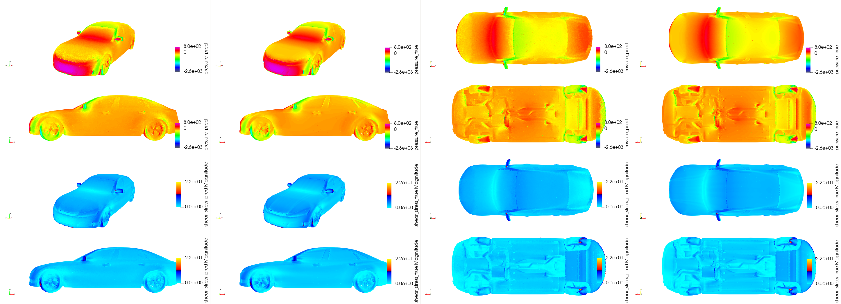
Figure 3: Comparison between the predictions and the ground truth for Sample 100. First two rows show pressure and last two rows show wall shear stress.

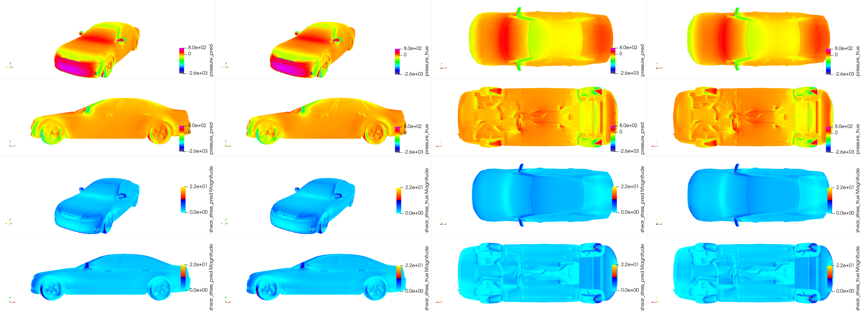
Figure 4: Comparison between the predictions and the ground truth for Sample 300. First two rows show pressure and last two rows show wall shear stress.

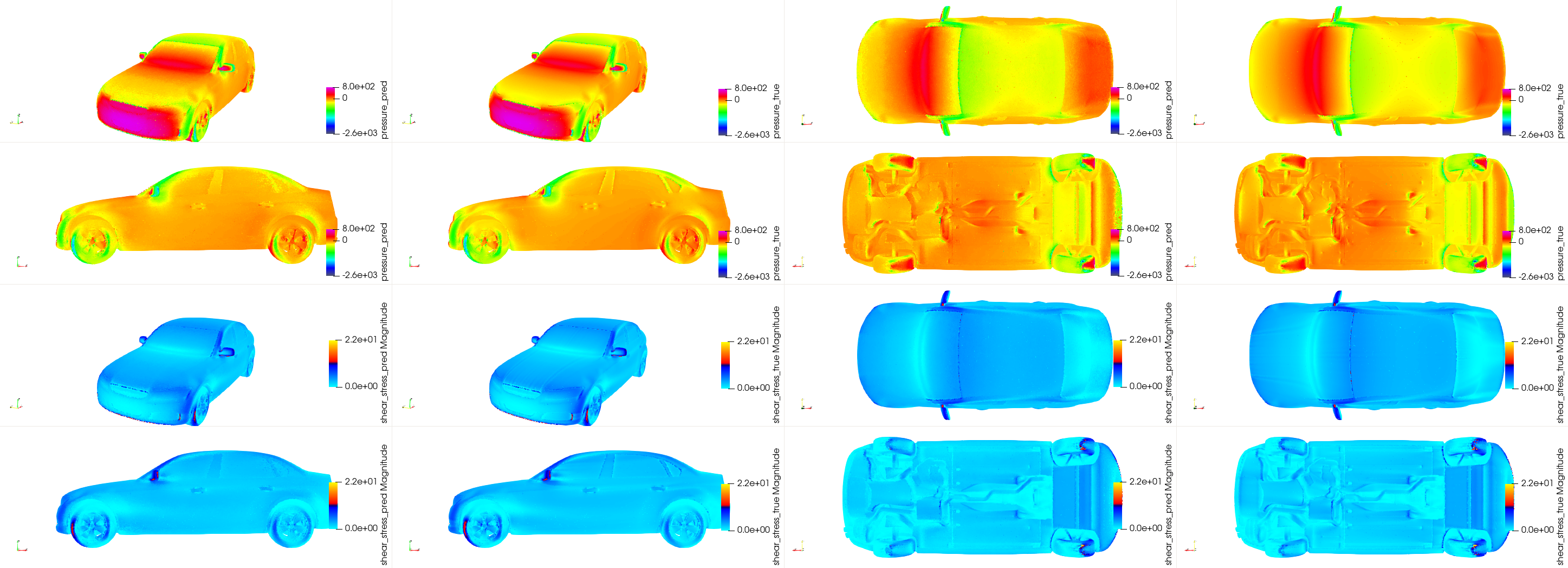
Figure 5: Comparison between the predictions and the ground truth for Sample 500. First two rows show pressure and last two rows show wall shear stress.

V-E Remarks

The application of X-MeshGraphNet to car aerodynamics highlights its ability to efficiently and accurately predict critical flow quantities, such as pressure and wall shear stress. By leveraging its scalable graph-based architecture and multi-scale graph construction, X-MeshGraphNet can handle complex surfaces with minimal computational overhead, offering a practical solution for automotive design and aerodynamics analysis.

V-F Ablation Study

A limited set of ablation studies was conducted to evaluate the sensitivity of the validation loss to various input variables. These studies included comparisons between a single-level graph and a 3-level graph, hidden sizes of 256 and 512, node degrees of 6 and 12, and training with or without input Fourier features. The results, shown in Figure 6 , indicate that both multi-level training and the inclusion of Fourier frequencies lead to a significant reduction in validation error.

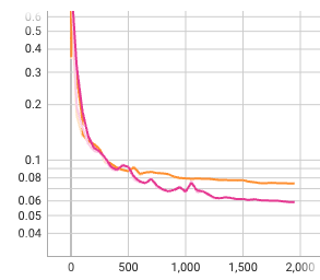
(a) 1 vs. 3* levels

(b) Hidden size of 256 vs. 512*

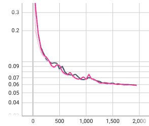
(c) Node degree of 6* vs. 12

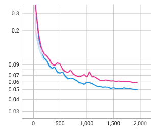
(d) W/* and w/o Fourier features

Figure 6: Validation loss for different configurations considered in the limited ablation study. Configurations resulting in lower validation error are marked with an asterisk (*).

VI Conclusion

In this paper, we introduced X-MeshGraphNet, a scalable multi-scale extension of the MeshGraphNet model, designed to address key challenges in GNN-based physical simulations. Our model overcomes the limitations of traditional GNNs in three critical areas: scalability, dependence on simulation meshes, and handling of long-range interactions.

First, X-MeshGraphNet scales to large simulations by partitioning the graph into smaller subgraphs, with halo regions facilitating seamless message passing across partitions. The use of gradient aggregation ensures that the partitioning does not compromise the accuracy or effectiveness of the training process, making it equivalent to training on the full graph while significantly reducing memory and computational overhead.

Second, to eliminate the time-consuming reliance on pre-generated simulation meshes, X-MeshGraphNet constructs custom graphs directly from CAD files. By generating uniform point clouds and connecting k-nearest neighbors, the model avoids the need for meshing, allowing for more efficient and flexible inference.

Third, the model introduces a multi-scale graph generation approach that captures both global and local dynamics by iteratively combining point clouds at different levels of resolution. This hierarchical representation ensures that X-MeshGraphNet can handle the complexities of multi-scale phenomena while remaining computationally efficient.

Our experiments demonstrate that X-MeshGraphNet can maintain the predictive accuracy of traditional GNN models while significantly improving scalability and flexibility. The model’s ability to handle large, complex simulations without requiring meshes at inference makes it particularly well-suited for real-time applications across various domains, from fluid dynamics to structural mechanics.

In future work, we aim to explore further optimizations in graph partitioning and edge connectivity strategies, as well as extend X-MeshGraphNet to handle a broader range of physical simulations, including those involving dynamic or deformable geometries. Additionally, integrating advanced physical constraints into the learning process may further improve the model’s accuracy and applicability to real-world systems.

Future work will also focus on exploring several extensions to further enhance the model’s flexibility and performance. One area of investigation will be comparing the effects of constructing graphs using the K-NN approach versus connecting points within a specified radius. Additionally, we plan to experiment with graph augmentation techniques, such as dynamically sampling point clouds and constructing the graph on the fly per epoch. This approach could help mitigate topological biases that arise from fixed graph structures.

Moreover, we intend to explore generating the point cloud non-uniformly, taking into account the curvature information of the geometry. By increasing point density in regions of high curvature, we expect to capture finer details more effectively, potentially improving the accuracy of the model in regions with complex phenomena.

Lastly, we plan to push the limits of scalability by training models with increasing numbers of graph nodes and edges. This will help us understand how far the scalability of X-MeshGraphNet can be practically extended in terms of handling larger graphs.

References

- [1] Battaglia, Peter W., Jessica B. Hamrick, Victor Bapst, Alvaro Sanchez-Gonzalez, Vinicius Zambaldi, Mateusz Malinowski, Andrea Tacchetti et al. ”Relational inductive biases, deep learning, and graph networks.” arXiv preprint arXiv:1806.01261 (2018).
- [2] Li, Yujia, Daniel Tarlow, Marc Brockschmidt, and Richard Zemel. ”Gated graph sequence neural networks.” arXiv preprint arXiv:1511.05493 (2015).
- [3] Pfaff, Tobias, Meire Fortunato, Alvaro Sanchez-Gonzalez, and Peter W. Battaglia. ”Learning mesh-based simulation with graph networks.” arXiv preprint arXiv:2010.03409 (2020).
- [4] Sanchez-Gonzalez, Alvaro, Jonathan Godwin, Tobias Pfaff, Rex Ying, Jure Leskovec, and Peter Battaglia. ”Learning to simulate complex physics with graph networks.” In International conference on machine learning, pp. 8459-8468. PMLR, 2020.
- [5] Karypis, George, and Vipin Kumar. ”A fast and high quality multilevel scheme for partitioning irregular graphs.” SIAM Journal on scientific Computing 20, no. 1 (1998): 359-392.
- [6] Li, Zongyi, Nikola Kovachki, Chris Choy, Boyi Li, Jean Kossaifi, Shourya Otta, Mohammad Amin Nabian et al. ”Geometry-informed neural operator for large-scale 3d pdes.” Advances in Neural Information Processing Systems 36 (2024).
- [7] Jacob, Sam Jacob, Markus Mrosek, Carsten Othmer, and Harald Köstler. ”Deep learning for real-time aerodynamic evaluations of arbitrary vehicle shapes.” arXiv preprint arXiv:2108.05798 (2021).
- [8] Elrefaie, Mohamed, Florin Morar, Angela Dai, and Faez Ahmed. ”DrivAerNet++: A Large-Scale Multimodal Car Dataset with Computational Fluid Dynamics Simulations and Deep Learning Benchmarks.” arXiv preprint arXiv:2406.09624 (2024).
- [9] Song, Binyang, Chenyang Yuan, Frank Permenter, Nikos Arechiga, and Faez Ahmed. ”Surrogate modeling of car drag coefficient with depth and normal renderings.” In International Design Engineering Technical Conferences and Computers and Information in Engineering Conference, vol. 87301, p. V03AT03A029. American Society of Mechanical Engineers, 2023.
- [10] Chen, Fangge, and Kei Akasaka. ”3D Flow Field Estimation around a Vehicle Using Convolutional Neural Networks.” In BMVC, p. 396. 2021.
- [11] Trinh, Thanh Luan, Fangge Chen, Takuya Nanri, and Kei Akasaka. ”3d super-resolution model for vehicle flow field enrichment.” In Proceedings of the IEEE/CVF Winter Conference on Applications of Computer Vision, pp. 5826-5835. 2024.
- [12] Tancik, Matthew, Pratul Srinivasan, Ben Mildenhall, Sara Fridovich-Keil, Nithin Raghavan, Utkarsh Singhal, Ravi Ramamoorthi, Jonathan Barron, and Ren Ng. ”Fourier features let networks learn high frequency functions in low dimensional domains.” Advances in neural information processing systems 33 (2020): 7537-7547.
- [13] Ashton, Neil, Charles Mockett, Marian Fuchs, Louis Fliessbach, Hendrik Hetmann, Thilo Knacke, Norbert Schonwald et al. ”DrivAerML: High-Fidelity Computational Fluid Dynamics Dataset for Road-Car External Aerodynamics.” arXiv preprint arXiv:2408.11969 (2024).