AUTO-IceNav: A Local Navigation Strategy for Autonomous Surface Ships in Broken Ice Fields

Abstract

Ice conditions often require ships to reduce speed and deviate from their main course to avoid damage to the ship. In addition, broken ice fields are becoming the dominant ice conditions encountered in the Arctic, where the effects of collisions with ice are highly dependent on where contact occurs and on the particular features of the ice floes. In this paper, we present AUTO-IceNav, a framework for the autonomous navigation of ships operating in ice floe fields. Trajectories are computed in a receding-horizon manner, where we frequently replan given updated ice field data. During a planning step, we assume a nominal speed that is safe with respect to the current ice conditions, and compute a reference path. We formulate a novel cost function that minimizes the kinetic energy loss of the ship from ship-ice collisions and incorporate this cost as part of our lattice-based path planner. The solution computed by the lattice planning stage is then used as an initial guess in our proposed optimization-based improvement step, producing a locally optimal path. Extensive experiments were conducted both in simulation and in a physical testbed to validate our approach.

I Introduction

Ice navigation is becoming of significant interest to the maritime sector due to a number of factors. Commercial shipping, for instance, has increasingly used the Arctic shipping routes in the last decade due to a reduction in ice cover [1]. The benefits of these alternative shipping routes include a decrease in emissions and a reduction in costs attributed to shorter travel times, reduced travel distances, and lower fuel consumption [2, 3, 4]. There is also interest in improving supply to Northern communities, ferry operations, Arctic patrol, and environmental monitoring by sea [5]. Despite these opportunities, the Arctic still presents considerable challenges and risks to safe and efficient navigation due to seasonally and regionally varying sea ice [6, 7, 8]. Sea ice conditions are affected by a range of different factors, both environmental (e.g., ocean currents and temperature) and operational (e.g., ship traffic and icebreaker assistance). This results in a wide variety of possible sea ice features that may be encountered during ship transit, each type presenting its own set of associated hazards [9].

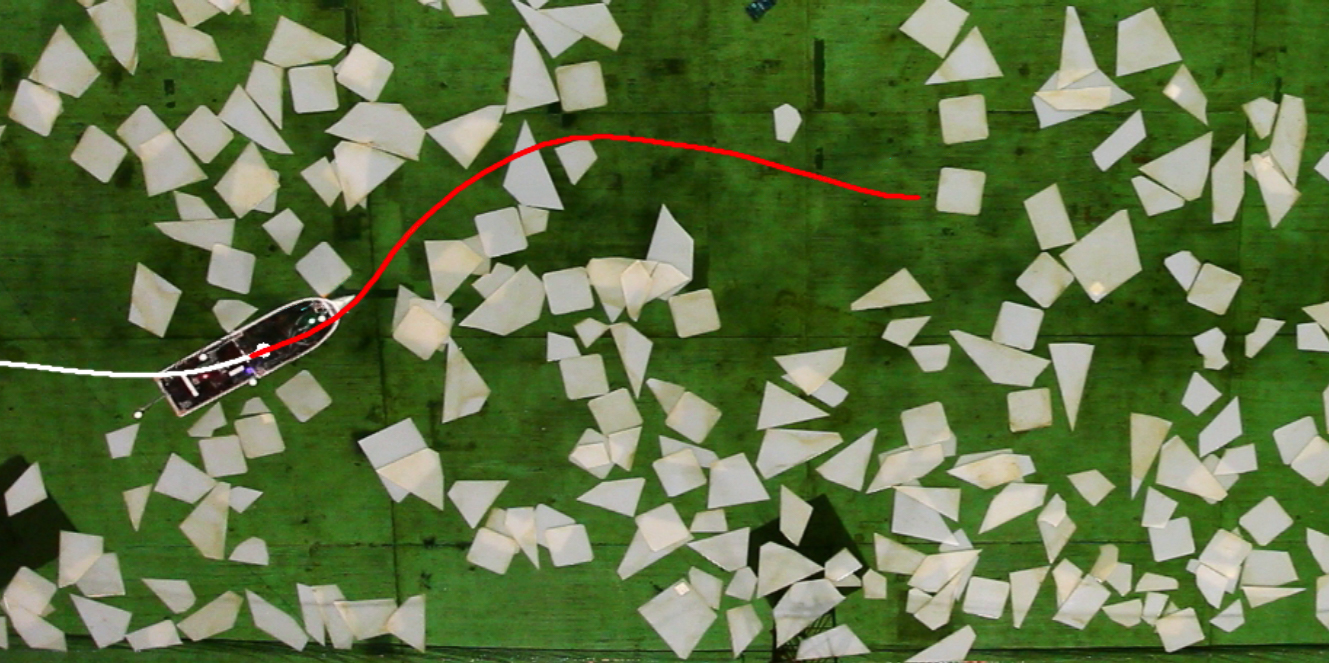
Figure 1: Snapshot of a sample trial from our physical experiments conducted in the Offshore Engineering Basin research facility in St. John’s, Newfoundland and Labrador.

Addressing the challenges of ice navigation fits well with the broader ongoing push toward greater ship autonomy and more intelligent systems to improve maritime safety and efficiency [10, 11, 12]. Although prior works have shown success in computing global routes that minimize ice navigation costs such as the average ice-induced forces exerted on the ship [13, 14], none have considered the problem of optimizing navigation at the local level where costs are computed based on individual ship-ice collisions. In this work, we address the problem of local navigation for the autonomous maneuvering of surface ships in ice-covered waters, making the following key assumptions: (i) the environment consists of broken sea ice, (ii) the ice concentration may be too high to achieve collision-free maneuvers, and (iii) the ship is rated for ice navigation but is not considered an icebreaker.

In contrast to level ice where continuous sheets are formed on the ocean surface requiring breaking of the ice, broken ice fields result in a much wider variety of possible ship-ice interactions [6]. Moreover, the most prevalent sea ice conditions expected to be encountered in the Arctic are ice floe fields [15, 16], and are the particular ice environments considered in this work (see Fig. 1). An ice floe field is defined as a collection of discrete floating ice pieces, called ice floes, which may be characterized by their thickness, size, and shape. Differences among floes in a given ice field often vary greatly in terms of size and shape [17, 18]. As a result, the collision responses vary significantly [15, 19, 20] and generally involve the ice floe being partially crushed and then pushed by the ship, leading to a loss of ship kinetic energy [8]. The problem of local navigation in broken ice fields thus requires a method for efficiently finding a sequence of maneuvers that can be executed by the ship and are optimized in terms of the modeled costs of the ship-ice collisions. We provide a solution to this task by considering a local planning problem in which collisions along a candidate plan are evaluated from a kinetic energy loss perspective based on the currently detected ice conditions.

In this paper, we extend our preliminary work [21] in the following ways. First, we present an extension to our cost function using an ice concentration representation of the ice conditions to account for scenarios where an additional cost is incurred from pushing ice floes not in direct contact with the ship. Next, we propose an optimization-based improvement step as a second stage to our planning approach that produces a locally optimal solution to the continuous path planning problem. In contrast to simulation experiments from [21], our experimental setup uses the dynamics of a full-scale vessel model, as well as a realistic distribution of ice floes and physics parameters. Our set of evaluation metrics includes statistics on the impact forces recorded during ship-ice collisions and the total energy consumption of the ship. The improved evaluation therefore captures a better picture of navigation performance, illustrating the trade-offs associated with changing course to avoid collisions with ice. In the physical experiments, we present quantitative results to complement the qualitative findings discussed in [21]. Finally, we release all code and documentation including our open source physics simulator for ship navigation in broken ice fields.

I-A Contributions

The following are the contributions of this work:

1. A method for autonomous real-time ship navigation of broken ice fields called AUTO-IceNav (Autonomous Two-stage Optimized Ice Navigation) which produces desirable ship maneuvers that avoid head-on collisions with larger ice floes and areas of higher ice concentration. We formulate an objective function for the total collision cost based on a kinetic energy loss formulation of the ship-ice interaction.

2. An optimization-based improvement step to locally refine the solution of a lattice-based planner, reducing the navigation cost in a two-stage path planning pipeline

3. An open source Python-based 2D simulator for efficient experimentation of full-scale ship transit in ice floe fields, addressing the current lack of any available open source physics simulators for ship operations in broken ice.

4. Results from extensive simulation experiments demonstrating our method’s ability to significantly reduce both the mean and maximum impact forces from ship-ice collisions and total energy consumption compared to naive navigation strategies.

5. Results from physical experiments conducted in a model-scale setup that show a 46% improvement in performance over prior work.

I-B Related Work

We review existing work relevant to our problem of interest, beginning with ship autonomy in ice navigation followed by related work on trajectory and motion planning in other maritime contexts. We note that while the problem of ice navigation shares similarities with a broader set of problems in robotics known as Navigation Among Movable Obstacles (NAMO) [22], the agent-obstacle interactions involve additional complexities (e.g., risk of damage to the agent and obstacles interacting with each other) when navigating among ice floes.

I-B1 Ship autonomy for ice navigation

Many studies have considered the task of optimizing a global route for ice navigation [23, 24, 6, 25, 26, 27, 14, 28, 13]. The goal in this task is to compute a sequence of waypoints from a starting position to a target destination that minimizes an objective function subject to a set of constraints. These routes are computed online and updated as necessary to provide ship captains with real-time guidance. However, these routes only provide navigational guidance at the global level and are optimized based on a coarse representation of the environment. For example, in [14, 28, 13], a discrete mesh is generated for each modality that describes the environmental conditions. Each cell in a particular mesh represents a subregion of the environment and is assigned a value corresponding to the specific input data (e.g., sea ice concentration) representing that region. Using ship performance models such as [6, 29], the mesh representation of the environment can be converted to a discrete map of navigation costs. Thus, the route planning problem can be efficiently solved by generating a graph from this discrete costmap. In our work, we follow a similar approach for representing the navigation cost, where we assign a collision cost to each cell in a fine grid representing the local ice conditions. Our cost function is also motivated by the objective functions typically considered in route planning but considers the cost at the level of individual ship-ice collisions along the path. Both the route planner and the local planner systems are required to achieve full ship autonomy [30].

Few studies consider the local planning task for ice navigation. In total, we found four previous works that tackle this problem [31, 4, 32, 33]. In [31, 4, 32], the authors propose a method for computing collision-free paths in broken ice environments. Although the authors of [31, 4] consider the turning radius constraints of the ship, the collision-free assumption limits the practical relevance of these works in ice navigation. Recall that a key assumption in our work is that the ice environment typically precludes collision-free navigation. The final local navigation approach we found is the shortest open water planning approach described in [33]. Here, the authors leverage the popular image processing technique, morphological skeletonization, to create a topological representation of the open water area from an overhead snapshot of the ice field. The information in the processed image is then extracted to build a graph from which a path is computed. Among these four related works [31, 4, 32, 33], the most practical method is [33] since it can easily be extended to high-concentration ice fields. As a result, we considered this approach as one of the baselines in our experiments.

I-B2 General ship autonomy

A larger body of work considers the broader task of autonomous ship operation in non-ice environments [34, 35, 36, 37, 38, 39, 40, 41, 42]. This includes urban waterways [40], harbors [43, 39], and shorelines [34]. In [40], a receding-horizon path planner is proposed for an autonomous ship operating in constrained urban environments. Since the obstacle environment is dynamic in nature, local planning is performed in an iterative fashion, where paths are continuously generated in real-time up to a small distance ahead of the ship’s current position. These paths should therefore account for the kinodynamic constraints of the vessel to be effectively followed. A challenge here is determining how to efficiently represent the space of feasible paths or, in the case of motion planning, the space of possible maneuvers that can be executed. Many methods address this problem by considering a discretization scheme. One popular technique is to define offline a finite set of optimized maneuvers as introduced in [44]. These maneuvers can be repeated in a particular sequence to produce a planned trajectory. The local planning problem can therefore be reduced to finding a cost-minimizing sequence of these maneuvers using graph search techniques [45]. In this work, we adopt the so-called state lattice planning approach to produce reference paths that consider the minimum turning radius constraints of the ship.

Treating local planning as a graph search problem has been shown to be an effective technique for autonomous ship navigation. In [39], the authors develop a two-stage optimization-based motion planner for ships navigating in confined environments (e.g., harbors). In the first stage, a lattice planner computes a trajectory by searching over a graph of motion primitives, while in the second stage, the authors formulate an optimal control problem which is warm-started with the lattice planning solution. This two-stage approach ensures that the computed plan is locally optimal with respect to the continuous planning problem. A similar method is proposed in [43], a key contribution being their novel encoding of polygonal obstacles into smooth and convex constraints. These works motivate our proposal for an optimization-based improvement step to enhance the path computed by the lattice planning stage in our ice navigation framework. We place particular emphasis on how we define a smooth objective function from the discrete collision cost formulated as part of the lattice planner stage.

II Preliminaries

II-A Notation and Ship Modeling

In this section, we introduce the notation used in this paper following the standard notation for the motion of a marine craft described in [10, 46]. The ocean surface on which a ship moves is treated as a 2D surface $\mathcal{W}\subseteq\mathbb{R}^{2}$. As such, it is sufficient to consider 3 degrees of freedom (DoF) for ship motion in the horizontal plane [10]. This corresponds to two translational movements, surge and sway, and one rotational movement, yaw, as shown in Fig. 2 (left). We use two reference frames to characterize the motion of the ship: an inertial frame $(x_{n},y_{n})$ and a body-fixed reference frame $(x_{b},y_{b})$ with the origin $o_{b}$ located at the center of gravity of the ship. The coordinates of $o_{b}$ expressed in the inertial frame give the position of the ship $(x,y)\in\mathbb{R}^{2}$. The direction in which the front of the ship points is referred to as the heading angle $\psi\in[0,2\pi)=\mathbb{S}^{1}$ which is defined by the angle from the inertial axis $x_{n}$ to the body-fixed axis $x_{b}$. Together, the position and heading are referred to as the generalized position or the pose of the ship, denoted $\bm{\eta}$ where

$$\bm{\eta}=\begin{bmatrix}x&y&\psi\end{bmatrix}^{\top}\in\mathcal{C}=\mathbb{R}^{2}\times\mathbb{S}^{1}.$$ (1)

The set $\mathcal{C}$ is considered the robot configuration space [45] of the ship. The velocity of the ship is expressed in the body-fixed reference frame. The three components are surge velocity $u$, sway velocity $v$, and yaw rate $r$. As a vector, the generalized velocity is represented by

$$\bm{\nu}=\begin{bmatrix}u&v&r\end{bmatrix}^{\top}\in\mathbb{R}^{3}.$$ (2)

We can compute $\sqrt{u^{2}+v^{2}}$ to obtain the speed $U\in\mathbb{R}$. The vectors $\bm{\eta}$, $\bm{\nu}$ are related via the kinematic relationship

$$\dot{\bm{\eta}}=\mathbf{R}(\psi)\bm{\nu},$$ (3)

where

$$\mathbf{R}(\psi)=\begin{bmatrix}\cos\psi&-\sin\psi&0\\ \sin\psi&\cos\psi&0\\ 0&0&1\end{bmatrix}$$ (4)

is the rotation matrix. A visual summary of the notation described above is provided in Fig. 2 (left).

Standard ship terminology is referenced in this work. The watertight body of the ship is called the hull and the front and rear parts are called the bow, and stern, respectively. The design of the hull varies greatly between different ship classes. In the case of ice-going vessels, the hull and other parts of the ship are reinforced to a certain level and are characterized by their assigned ice class [7]. Given particular ice conditions, the ice class of a ship is useful to determine a safe vessel speed under which the expected ice resistance forces remain within an acceptable level.

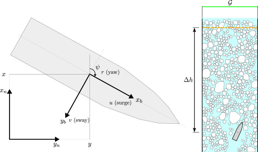
Figure 2: (Left) The two coordinate systems used to describe ship motion in three degrees of freedom. (Right) Depiction of the navigation problem of interest for a ship navigating a cluttered ice channel where the high-level objective is forward progress along the channel.

II-B Problem Formulation

We consider the task of navigating a ship through a broken ice field modeled as a rectangular ice channel $\mathcal{I}\subseteq\mathcal{W}$. Without loss of generality, the channel length is assumed to be aligned with the $x_{n}$ axis of the inertial frame as in Fig. 2 (right). The high-level objective is for the ship to make forward progress along the ice channel. As such, we consider a line segment perpendicular to the channel length as the navigation goal $\mathcal{G}$, defined in the configuration space $\mathcal{C}$, as follows:

$$\mathcal{G}=\{\bm{\eta}\in\mathcal{C}\mid(x,y)\in\mathcal{I},x=x_{\text{goal}}\},$$ (5)

with parameter $x_{\text{goal}}$ denoting the $x$ coordinate of the goal. Note that while we treat the navigation area as rectangular, it is possible to adapt our method to other environment shapes.

Suppose a top-down view of the ice field is actively captured with sensors mounted on board and processed via an ice image processing system [18]. Given $m$ ice floes observed in the environment, each floe is treated as an obstacle with a footprint $\mathcal{O}_{i}\subset\mathcal{I}$ occupying space in the 2D environment, where $i=1,\dots,m$. Using the footprints, we can extract important ice properties, including shape and size [18]. Let $\mathcal{W}_{\text{obs}}=\{\mathcal{O}_{1},\dots,\mathcal{O}_{m}\}$ denote the collection of all ice floes and let $\mathcal{W}_{\text{free}}$ denote the corresponding open water area defined as the set difference $\mathcal{I}\setminus\bigcup_{i}\mathcal{O}_{i}$. The notion of a footprint is also useful for characterizing the region in $\mathcal{I}$ occupied by the ship at a pose $\bm{\eta}$, denoted as $\mathcal{F}(\bm{\eta})\subset\mathcal{I}$.

To navigate a ship, we require the following: a reference path $\bm{\pi}:\mathbb{R}\rightarrow\mathcal{C}$ parameterized by arc length $s\in[0,L_{f}]$ with total path length $L_{f}$, a velocity profile $\bm{\mathrm{v}}:\mathbb{R}\rightarrow\mathbb{R}^{3}$ that describes how the path is traversed over time, and a controller that tracks the path at the specified velocity. Let the tuple $(\bm{\pi},\bm{\mathrm{v}})$ denote a trajectory. To capture the navigation cost of a trajectory $(\bm{\pi},\bm{\mathrm{v}})$, we define an objective function $J$ as

$$J=T_{f}+\alpha C_{f},$$ (6)

which penalizes a weighted sum of the total travel time $T_{f}$ and the total collision cost $C_{f}$, weighted by the parameter $\alpha\geq 0$. Although the precise form of $C_{f}$ will be discussed later, we propose that a suitable function for the cost incurred from ship-ice collisions should accumulate a collision cost $c_{\text{obs}}\geq 0$ as the ship, characterized by its footprint $\mathcal{F}$, follows a trajectory $(\bm{\pi},\bm{\mathrm{v}})$ through an ice channel containing ice floes $\mathcal{W}_{\text{obs}}$. Thus, we seek to solve the following problem.

Problem 1 (Ice Navigation Trajectory Planning Problem).

Given an initial pose $\bm{\eta}_{\textnormal{cur}}$, a goal $\mathcal{G}$, ice floes $\mathcal{W}_{\textnormal{obs}}$, a ship with a footprint $\mathcal{F}$, and an ice channel $\mathcal{I}$, compute a trajectory $(\bm{\pi},\bm{\mathrm{v}})$ from $\bm{\eta}_{\textnormal{cur}}$ to $\mathcal{G}$ that minimizes $J$ and such that $\bm{\mathrm{v}}$ is bounded above by a safe vessel speed.

In what follows, we propose a solution to Problem 1 and describe how it is incorporated into a navigation system.

III Navigation Framework

We present a navigation framework and an overview of our approach to solving Problem 1. To account for the large and evolving environment, we frequently replan a reference path and velocity profile for a controller in real-time. Replanning is performed over a moving horizon, as illustrated by the part of the channel lying below the orange dotted line in Fig. 2 (right).

Algorithm 1 AUTO-IceNav

Input: $\mathcal{G},\Delta h,\Delta t$

1:while True do

2:     $\bm{\eta}_{\textnormal{cur}}\leftarrow$ Current ship pose

3:     if $\bm{\eta}_{\textnormal{cur}}$ has not crossed $\mathcal{G}$ then

4:         Obtain $\mathcal{W}_{\text{obs}}$ and set subgoal $\mathcal{G}_{\text{int}}$ given $\Delta h$, $\bm{\eta}_{\textnormal{cur}}$

5:         $U_{\text{nom}}\leftarrow$ Nominal speed given $\mathcal{W}_{\text{obs}}$

6:         $c_{\text{obs}}^{(1)}\leftarrow$ KE cost given $\mathcal{W}_{\text{obs}}$, $U_{\text{nom}}$ // Sec IV-A2

7:         $c_{\text{obs}}^{(2)}\leftarrow$ Ice coverage cost given $\mathcal{W}_{\text{obs}}$ // Sec IV-A3

8:         $\mathcal{C}_{\text{map}}\leftarrow$ Costmap given $c_{\text{obs}}^{(1)}c_{\text{obs}}^{(2)}$ // Eq. 9     

9:         $\bm{\pi}\leftarrow$ Path $\bm{\eta}_{\textnormal{cur}}\leadsto\mathcal{G}_{\text{int}}$ given $\mathcal{C}_{\text{map}}$ // Sec IV  

10:         $\bm{\pi}_{\text{opt}}\leftarrow$ Optimized path given $\bm{\pi}$, $\mathcal{C}_{\text{map}}$ // Sec V   

11:         $\bm{\mathrm{v}}_{\text{nom}}\leftarrow$ Velocity profile for $\bm{\pi}_{\text{opt}}$ given $U_{\text{nom}}$

12:         Send $(\bm{\pi}_{\text{opt}},\bm{\mathrm{v}}_{\text{nom}})$ to controller to track for time $\Delta t$

13:     else

14:         Exit loop      

The navigation framework is summarized in Algorithm 1, which takes as input a final goal $\mathcal{G}$, a receding horizon parameter $\Delta h$, and a tracking duration parameter $\Delta t$. At the start of each iteration, we obtain the current pose $\bm{\eta}_{\textnormal{cur}}$ and the updated ice floe information $\mathcal{W}_{\text{obs}}$ from the vision system (Lines 2, 4) — we assume that other important ice properties may be queried at this stage, including the ice thickness and ice density, but it is often sufficient to treat these as constant for a given local region [13]. Using this new information, we update the horizon planning window and set a new limit $U_{\text{nom}}$ on the nominal safe speed (Lines 4, 5). The intermediate goal $\mathcal{G}_{\text{int}}$ is set at a distance $\Delta h$ ahead of the ship’s position.

The core of our proposed framework lies in Lines 6-10 of Algorithm 1. Given the observed ice floes $\mathcal{W}_{\text{obs}}$ and the current nominal speed $U_{\text{nom}}$, we compute a costmap $\mathcal{C}_{\textup{map}}$ based on two different penalties associated with collisions involving the ice floes. In Line 6, we calculate a cost based on the ship’s kinetic energy loss to penalize direct contact with ice floes, while in Line 7, we apply an additional penalty based on the ice concentration. Using a lattice-based planner, we can efficiently compute the total collision cost $C_{f}$ using the costmap $\mathcal{C}_{\textup{map}}$. In Line 9, the lattice planner plans a reference path $\bm{\pi}$ from the current ship pose $\bm{\pi}(0)=\bm{\eta}_{\textnormal{cur}}$ to somewhere along the intermediate goal $\bm{\pi}(L_{f})\in\mathcal{G}_{\text{int}}$. From here, we locally optimize the planned path using our proposed optimization-based improvement step (Line 10). Since the path planning stage assumes that the ship is traveling at the nominal speed $U_{\text{nom}}$, we see that the travel time $T_{f}$ is equal to $L_{f}/U_{\text{nom}}$. Hence, our planning algorithm minimizes an objective that is equivalent to minimizing (6):

$$J=L_{f}+\alpha C_{f}.$$ (7)

In the final steps, the velocity profile $\bm{\mathrm{v}}_{\text{nom}}$ is generated for the optimized path (Line 11) and the controller tracks the planned trajectory $(\bm{\pi}_{\text{opt}},\bm{\mathrm{v}}_{\text{nom}})$ for time $\Delta t$ (Line 12). We discuss our implementation of these two final steps as part of the experimental setup in Section VI.

The steps described above are repeated until the ship reaches the goal $\mathcal{G}$. Note that in each planning iteration, the ice is treated as static when computing a trajectory $(\bm{\pi}_{\text{opt}},\bm{\mathrm{v}}_{\text{nom}})$. However, we frequently perform planning updates to account for ship-ice collisions that cause changes in the ice environment over short periods of time. As a result, we maintain low runtime in our path planning algorithm. The following sections describe the two stages of our proposed path planning pipeline.

IV Path Planning using a State Lattice

The lattice-based planner from [44] is adopted for our path planner, where planning is cast as a search problemecomputed finite set of actions, characterized by a set of differential equations, is defined such that applying repeated actions generates a regularly repeating arrangement, or lattice, of states. More precisely, we require a control set $\mathcal{P}$ where each motion primitive $\bm{\pi}\in\mathcal{P}$ can generate a path $\bm{\pi}$ such that $\bm{\pi}(0)=p_{0}\in L$ of the lattice $L$ and $\bm{\pi}(L_{f})=p_{1}\in L$. For an appropriately defined control set $\mathcal{P}$, we can construct a graph $G^{\mathcal{P}}=(L,E,w)$ with vertices $L$, edges $E$, and a function $w:E\rightarrow\mathbb{R}$ to assign edge costs. Each edge that connects a pair of vertices $(p_{0},p_{1})$ is the result of rotating and translating (in robot configuration space) a particular motion primitive. In addition, since the control set is defined using a particular model of the robot motion characteristics, a sequence of concatenated primitives will by construction produce a feasible path, or in other words, a path that satisfies the robot model. We can therefore use popular graph search techniques to efficiently plan cost-minimizing feasible paths in the graph $G^{\mathcal{P}}$.

We discuss how the above-mentioned state lattice framework is applied to our path planning problem. Following several other works in ship navigation on a 2D surface [47, 42, 48, 49], we assume paths generated by a ship can be approximated by a unicycle model where the curvature $\kappa$ is constrained to a limit $\kappa_{\max}$:

$$\begin{split}\dot{\bm{\eta}}(s)&=\begin{bmatrix}\dot{x}\\ \dot{y}\\ \dot{\psi}\end{bmatrix}=\begin{bmatrix}\cos(\psi)\\ \sin(\psi)\\ \kappa\end{bmatrix}\\ |\kappa|&\leq\kappa_{\max}.\end{split}$$ (8)

Here, the derivatives $\dot{(\cdot)}$ are taken with respect to arc length $s$. We set the limit $\kappa_{\max}$ based on the physical limits of the ship given the particular conditions in the environment and the nominal speed $U_{\text{nom}}$ [7, 10]. This limit is typically expressed in terms of the minimum turning radius of the ship, $r_{\min}$, where $r_{\min}=\kappa_{\max}^{-1}$.

Given $\eqref{eq:unicycle}$, we can consider the discretization of the configuration space $\mathcal{C}$. We generate a state lattice $L$ by discretizing the plane $\mathbb{R}^{2}$ into a uniform grid and the unit circle $\mathbb{S}^{1}$ into uniformly spaced angles. In each iteration of Algorithm 1, we build a graph $G^{\mathcal{P}}$ with a lattice $L$ initialized at the current pose of the ship $\bm{\eta}_{\textnormal{cur}}$. To define our motion primitives, we compute shortest paths between states $\bm{\eta}=[x\ y\ \psi]^{\top}$ for the unicycle model (8), known as Dubins’ paths [50]. These paths consist of sequences of straight lines and circular arcs of radius $r_{\min}$. Ideally, we would like to have a minimum turning radius $r_{\min}$ that accurately reflects the current nominal speed $U_{\text{nom}}$ from Algorithm 1. However, since the motion primitives are defined offline, we can instead generate a suite of control sets with different minimum turning radii and then select online the best matching control set and $r_{\min}$ for the given $U_{\text{nom}}$. The control set $\mathcal{P}$ (or a series of control sets with different $r_{\min}$) is generated using the method proposed in [51]. The edges of the graph are assigned a cost equal to our objective function $\eqref{eq:nav_framework_J_cost}$ where the total collision cost $C_{f}$ is described in detail in the next section. The A* graph search algorithm [52] is used to plan a path $\bm{\pi}$ from the current pose $\bm{\eta}_{\textnormal{cur}}$ to the current goal $\mathcal{G}_{\text{int}}$. In Section IV-B, we present an admissible heuristic to improve the performance of A*.

IV-A Total Collision Cost

If we assume ice-free conditions, the path length $L_{f}$ provides an approximate model for the ship’s energy consumption in a local region where other environment conditions are likely less variable. As a result, for the total collision cost $C_{f}$ we use the notion of total kinetic energy loss during ship-ice collisions to capture the additional cost incurred during navigation. We start by describing how we can efficiently compute the cost of a candidate path, $\bm{\pi}$, given obstacles, $\mathcal{W}_{\text{obs}}$, in a lattice-based planner.

IV-A1 Costmap representation of the environment

The ice channel $\mathcal{I}$ is discretized into a uniform grid with resolution $\Delta_{\text{grid}}$ where each grid cell is assigned an identifying tuple $\bm{k}\in\mathbb{N}^{2}$ corresponding to the position of the grid cell’s center. We use a subscript ‘d’ to distinguish between the continuous and discrete representations. Let $\mathcal{I}_{d}\subseteq\mathbb{N}^{2}$ denote the discretized ice channel. Each ice floe is mapped to a discrete footprint $\mathcal{O}\subset\mathcal{I}_{d}$ and we denote $\mathcal{W}_{\text{obs},d}$ as the set of obstacle discrete footprints. Each grid cell $\bm{k}$ is an element of at most one obstacle footprint $\mathcal{O}\in\mathcal{W}_{\text{obs},d}$ and $\bm{k}$ is considered an element of an obstacle $\mathcal{O}$ if the continuous footprint representation covers any part of the cell.

Using this discrete representation of the planar environment, we can generate a costmap $\mathcal{C}_{\textup{map}}:\mathcal{I}_{d}\rightarrow\mathbb{R}_{\geq 0}$ [44] by assigning a collision cost to each grid cell using our proposed collision cost function, $c_{\text{obs}}$. Given the nominal speed $U_{\text{nom}}$ and the obstacles $\mathcal{W}_{\text{obs},d}$, the cost at a grid cell $\bm{k}$ is defined as

$$c_{\text{obs}}(\bm{k},U_{\text{nom}},\mathcal{W}_{\text{obs},d})=\begin{cases}c_{\text{obs}}^{(1)}c_{\text{obs}}^{(2)},&\exists\mathcal{O}\mid\bm{k}\in\mathcal{O}\\ 0&\text{otherwise},\end{cases},$$ (9)

where $c_{\text{obs}}^{(1)}$ is the kinetic energy loss penalty (Section IV-A2) and $c_{\text{obs}}^{(2)}$ is the ice concentration penalty (Section IV-A3). Observe that (9) results in a costmap with nonzero costs only at grid cells that overlap with an obstacle.

To compute the cost of being at the pose $\bm{\eta}$ we require an appropriate mapping from the configuration space to $\mathcal{I}_{d}$ as well as a footprint $\mathcal{F}_{d}(\bm{\eta})\subset\mathbb{N}^{2}$ specifying the set of grid cells occupied by the ship body given the current position and heading. The total collision cost for a path $\bm{\pi}$ is computed as a sum over the set of costmap grid cells $\mathcal{S}(\bm{\pi})\subset\mathcal{I}_{d}$ swept by the ship footprint $\mathcal{F}_{d}$ from tracing the path $\bm{\pi}$. The set $\mathcal{S}(\bm{\pi})$ is referred to as the swath [44] of the path $\bm{\pi}$, and we show an example in Fig. 3. Hence, we compute the total collision cost $C_{f}$ as the swath cost:

$$C_{f}=\sum_{\bm{k}\in\mathcal{S}(\bm{\pi})}c_{\text{obs}}(\bm{k},U_{\text{nom}},\mathcal{W}_{\text{obs},d}).$$ (10)

Remark 1 (Obstacle Proximity Penalty).

In contrast to typical cost functions used in navigation problems, (10) does not apply a penalty for being in proximity to obstacles that are not in collision with the path. In our particular problem, planning paths arbitrarily close to obstacle edges (particularly large ice floes) without penalty may not be desirable behavior, especially considering that we expect some error in tracking. To address this, a straightforward extension is to scale up the obstacle footprints $\mathcal{W}_{\text{obs}}$ by a small factor (e.g., 0.1) proportional to their size. This would effectively generate a cost buffer around the ice floes in the costmap. Regarding the potential issue of having overlap between multiple scaled-up obstacle footprints, the solution used here is to assign the maximum of the costs computed for a grid cell $\bm{k}$.

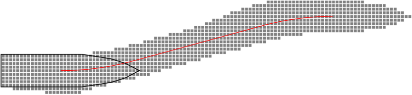
Figure 3: The swath (grey grid cells) of a sample path (red line) and ship footprint (black outline). In this example, each cell in the discretized channel represents a region of size 2 m $\times$ 2 m.

IV-A2 Kinetic energy loss penalty

We present the kinetic energy loss penalty $c_{\text{obs}}^{(1)}$ from (9). We consider a simple 2D ship-ice collision model and show a derivation of the kinetic energy loss of the ship from the collision. More complex ship-ice interactions, such as floe-splitting and rafting behavior [17], are ignored.

Let $m_{\text{ship}}$ and $m_{\text{ice}}$ denote the mass of the ship and ice floe, respectively. We assume that ice floes have uniform density and thickness. Thus, the mass $m_{\text{ice}}$ is given by the product of density, thickness, and area of the ice floe [20], where the area is determined by the extent of its footprint $\mathcal{O}\in\mathcal{W}_{\text{obs}}$ (usually a convex polygon). Similar to the collision model proposed in [20] and then experimentally validated in [53, 54], we reduce the collision to a one-body problem by making the following assumptions: the collision is of short duration, the momentum of the system is conserved (i.e., friction is ignored), and the impact force is normal to the line of contact between the two bodies (see Fig. 4 (left)). In addition, the collision is assumed to be inelastic, where the maximum amount of kinetic energy of the system is lost to ice crushing [55, 20].

With this collision model, the change in kinetic energy $\Delta K_{\text{sys}}$ in the system is given by

$$\Delta K_{\text{sys}}=-\frac{1}{2}M_{\text{eq}}V_{\text{eq}}^{2},$$ (11)

where $M_{\text{eq}}$, called effective mass, is the mass in the center of mass frame, and $V_{\text{eq}}$ is the relative velocity of the two bodies before the collision with respect to the line of contact. If we consider two disk-shaped bodies, the effective mass is only a function of the two masses:

$$M_{\text{eq}}=\frac{m_{\text{ship}}m_{\text{ice}}}{m_{\text{ship}}+m_{\text{ice}}}.$$ (12)

From [55], the ice velocity is assumed to be negligible compared to the ship velocity. Hence, the relative velocity $V_{\text{eq}}$ is a function of the ship speed $U$ and the angle $\theta$ between the direction in which $U$ is pointing and the vector normal to the line of contact:

$$V_{\text{eq}}=U\cos(\theta).$$ (13)

The angle $\theta$ is illustrated in Fig. 4 (left). Next, we isolate the change in kinetic energy of the ship $\Delta K_{\text{ship}}$.

The goal of our collision cost will be to minimize the kinetic energy loss of the ship due to the kinetic energy transferred to the ice and absorbed by ice crushing. Since the ice is treated as static prior to collision, it must hold that the change in kinetic energy of the ice $\Delta K_{\text{ice}}$ is greater than 0. In summary, we have the inequalities

$$\Delta K_{\text{sys}}<0,\quad\Delta K_{\text{ice}}>0,\quad\Delta K_{\text{ship}}<0,$$ (14)

as well as the following relationship between the changes in kinetic energy for the ship, ice, and system:

$$\Delta K_{\text{sys}}=\Delta K_{\text{ice}}+\Delta K_{\text{ship}}.$$ (15)

After the collision has occurred, we treat the ice floe as having a final velocity equal to $V_{\text{eq}}m_{\text{ship}}(m_{\text{ship}}+m_{\text{ice}})^{-1}$. Therefore,

$$\begin{split}\Delta K_{\text{ice}}&=\frac{1}{2}m_{\text{ice}}\left(\frac{V_{\text{eq}}m_{\text{ship}}}{m_{\text{ship}}+m_{\text{ice}}}\right)^{2}\\ &=\frac{1}{2}\frac{m_{\text{ice}}m_{\text{ship}}^{2}}{(m_{\text{ship}}+m_{\text{ice}})^{2}}(U\cos(\theta))^{2}\end{split}$$ (16)

and from (11) (15):

$$\Delta K_{\text{ship}}=-\frac{m_{\text{ice}}m_{\text{ship}}(m_{\text{ice}}+2m_{\text{ship}})}{2(m_{\text{ice}}+m_{\text{ship}})^{2}}(U\cos(\theta))^{2}.$$ (17)

Figure 4: (Left) The collision model of two disk-shaped bodies used to derive the cost function. (Right) An example of a costmap with a grid cell size of 1 m $\times$ 1 m. Brighter colors indicate higher cost. The centroid of each ice floe is indicated by the red ‘x’ and the bounding circles are shown in light blue. In this example, the ice thickness and density is the same across ice floes meaning the size of the polygon corresponds to its mass.

Suppose that the disk representing the ice floe has a radius of $r_{\text{ice}}$ and a center located at $\bm{c}_{\text{ice}}\in\mathbb{R}^{2}$. The angle $\theta$ in the expression (17) can be written in terms of $r_{\text{ice}}$ and the lateral distance $d$ between $\bm{c}_{\text{ice}}$ and the center of the line of contact (this is also where the impact force is exerted) measured with respect to the component parallel to the direction of $U$. From Fig. 4 we have,

$$\theta=\arcsin\left(\frac{d}{r_{\text{ice}}}\right).$$ (18)

As a result, given a particular ship with constant mass $m_{\text{ship}}$, $\Delta K_{\text{ship}}$ from (17) can be written as a function of $d$, $r_{\text{ice}}$, $m_{\text{ice}}$, and $U$:

$$\begin{split}&\Delta K_{\text{ship}}(d,r_{\text{ice}},m_{\text{ice}},U)=\\ &=\frac{m_{\text{ice}}m_{\text{ship}}(m_{\text{ice}}+2m_{\text{ship}})}{2(m_{\text{ice}}+m_{\text{ship}})^{2}}\left[U\cos\left(\arcsin\left(\frac{d}{r_{\text{ice}}}\right)\right)\right]^{2}\\ &=\frac{U^{2}m_{\text{ice}}m_{\text{ship}}(m_{\text{ice}}+2m_{\text{ship}})}{2(m_{\text{ice}}+m_{\text{ship}})^{2}}\left(\frac{r_{\text{ice}}^{2}-d^{2}}{r_{\text{ice}}^{2}}\right),\quad d\in[0,r_{\text{ice}}].\end{split}$$ (19)

Here, we have omitted the negative sign so that now $\Delta K_{\text{ship}}$ denotes the kinetic energy loss of the ship. Finally, consider a cell $\bm{k}$ and assume there exists an ice floe $\mathcal{O}_{j}\in\mathcal{W}_{\text{obs},d}$ such that $\bm{k}\in\mathcal{O}_{j}$. Let $\bm{c}_{\text{ice},j}$ denote the position of the centroid of $\mathcal{O}_{j}$, $r_{\text{ice},j}$ the radius of its bounding circle centered at $\bm{c}_{\text{ice},j}$, and $m_{\text{ice},j}$ its mass. The kinetic energy loss penalty for cell $\bm{k}$ given current nominal speed $U_{\text{nom}}$ is defined as

$$\begin{split}&c_{\text{obs}}^{(1)}=\Delta K_{\text{ship}}(d^{\prime},r_{\text{ice},j},m_{\text{ice},j},U_{\text{nom}}),\end{split}$$ (20)

where $d^{\prime}=||\bm{k}-\bm{c}_{\text{ice},j}||$ is the Euclidean distance from the grid cell $\bm{k}$ to the centroid $\bm{c}_{\text{ice},j}$ of the obstacle $\mathcal{O}_{j}$. Fig. 4 (right) illustrates a sample costmap and shows the bounding circles and radii of the obstacles.

Observation 1 (Large Obstacles and Head-On Collisions).

Given the swath $\mathcal{S}(\bm{\pi})$ of a path $\bm{\pi}$, clearly from (19), (20) a larger penalty is applied if the swath overlaps ice floes with larger mass. In addition, the cost of the swath increases as the grid cells $\bm{k}\in\mathcal{S}(\bm{\pi})$ become closer to the centroid of an obstacle. This is particularly visible in Fig. 4 in the ice floes that are less circular (e.g., rectangular shaped), where the edges of the shape that are closer to the centroid are assigned a higher cost than the edges farther away. In practice, this means that paths with fewer head-on collisions with large ice floes are favored during planning. This typically results in the ship pushing the ice floes off to the side during navigation with few instances of sustained contact. As expected, collisions with larger ice floes and collisions that are more head-on result in larger impact forces exerted on the ship [7, 20].

IV-A3 Ice concentration penalty

In the ice concentration penalty $c_{\text{obs}}^{(2)}$ from (9), our goal is to account for scenarios where the ship displaces a greater amount of ice than the set of ice floes that were in direct contact with the ship. More formally, for a given path $\bm{\pi}$ and a corresponding swath $\mathcal{S}(\bm{\pi})$, there may exist a set of obstacles $\{\mathcal{O}_{j}\}_{j=1}^{n}\subset\mathcal{W}_{\text{obs},d}$, where $n>0$, and where for each $\mathcal{O}_{j}$ we have $\mathcal{O}_{j}\cap\mathcal{S}(\bm{\pi})=\emptyset$, and yet each $\mathcal{O}_{j}$ creates additional resistance to ship motion, resulting in an increase in kinetic energy loss. Such scenarios are more likely to occur as the concentration of the ice field increases. Moreover, in [29] the relationship between the average ice resistance force exerted on the ship and the ice concentration $C_{\text{ice}}\in[0,1]$ is modeled as a linear function in $(C_{\text{ice}})^{\beta}$ where $\beta\geq 1$ is a constant parameter determined by the geometry of the particular ship hull.

To assign an ice concentration cost to grid cells in the costmap, we first generate a binary occupancy image of the ice channel from $\mathcal{W}_{\text{obs},d}$ indicating the pixels that are occupied by an ice floe. We then compute an image convolution between the binary image and a mean filter with kernel size $z\times z$, where $z$ is odd. For a given pixel $\bm{k}\in\mathbb{N}^{2}$ in the binary image, the mean filter will compute the average ice concentration for a region of size $z\times z$ in pixel units centered around $\bm{k}$. For the purpose of local navigation, the kernel should therefore be appropriately sized so that at a given location the extent of the kernel can capture a collection of ice floes in a region that is still relatively local compared to the rest of the ice channel. The resulting image, $C_{\text{ice}}:\mathbb{N}^{2}\rightarrow[0,1]$, provides a smooth representation of the ice concentration at every position in the discretized ice channel $\mathcal{I}_{d}$. This contrasts with the coarse grid or mesh representation [13], where each cell represents a large area and is assigned a single ice concentration value, which is more suitable for route planning.

Note that we apply mirror padding to the binary image prior to computing $C_{\text{ice}}$ to prevent the loss of ice information at the boundaries of the image. Given the obstacles $\mathcal{W}_{\text{obs},d}$, the ice concentration penalty for a cell $\bm{k}$ is defined as

$$c_{\text{obs}}^{(2)}=(C_{\text{ice}}(\bm{k}))^{\beta}.$$ (21)

IV-B Heuristic

To improve the runtime of A* search during path planning, we propose an admissible heuristic $h$. Given the two terms in (7), we can compute two separate heuristics, each admissible with respect to a term in the cost. Specifically, we require a function $h_{1}(\bm{\eta})$ such that it lower bounds the path length $L_{f}$ and another function $h_{2}(\bm{\eta})$ such that it lower bounds the total collision cost $C_{f}$ for all $\bm{\eta}$ given the current goal $\mathcal{G}_{\text{int}}$ and costmap $\mathcal{C}_{\textup{map}}$. We can therefore do a summation to get an admissible function $h(\bm{\eta})$:

$$h(\bm{\eta})=h_{1}(\bm{\eta})+\alpha h_{2}(\bm{\eta}).$$ (22)

We refer to the two terms in $h$ as the nonholonomic without obstacles heuristic [56, 43] and the obstacles-only heuristic, respectively.

IV-B1 Nonholonomic without obstacles

Path length $L_{f}$ is lower bounded by the length of the shortest path from $\bm{\eta}$ to an infinite line $\mathcal{G}_{\infty}$ that is collinear with the intermediate goal $\mathcal{G}_{\text{int}}$, subject to the unicycle model (8). Recall our definition of the goal in (5) and recall our world coordinate frame shown in Fig. 2. To characterize the proposed heuristic, we offer the following result.

Theorem 1 (Closed-form Heuristic for Path Length).

The shortest path from $\bm{\eta}=[x\ y\ \psi]^{\top}$ to the infinite straight line segment $\mathcal{G}_{\infty}$ with minimum turning radius $r_{\min}$ is a Dubin’s path. Referencing Fig. 5,

1. if $\mathcal{G}_{\infty}$ lies above the point $\bm{c}=[x_{c}\ y_{c}]^{\top}$, the path is of the form CS (circular arc C of radius $r_{\min}$, followed by a straight line segment S) and S intersects $\mathcal{G}_{\infty}$ at $\theta=\pi/2$ (Fig. 5 (left));

2. otherwise, the path is of the form C (Fig. 5 (right)).

Given these two cases, $h_{1}(\bm{\eta})$ is the path length and is given analytically by:

$$\begin{split}h_{1}(\bm{\eta})&=\begin{cases}h_{a}(\bm{\eta}),\ &\text{if }x_{c}\leq x_{\text{goal}}\ \text{(case a)},\\ h_{b}(\bm{\eta}),\ &\text{otherwise (case b)}\end{cases},\\ \text{where}&\\ h_{a}(\bm{\eta})&=r_{\min}\left|\frac{\pi}{2}-\phi\right|+x_{\text{goal}}-x_{c}\\ h_{b}(\bm{\eta})&=r_{\min}\left|\phi-\arccos\left(\frac{x_{c}-x_{\text{goal}}}{r_{\min}}\right)\right|\\ x_{c}&=x+r_{\min}\left|\cos(\phi)\right|\\ \end{split}$$

and where $\phi\in[-\frac{\pi}{2},\frac{\pi}{2}]$ is the heading measured with respect to the line segment $\mathcal{G}_{\infty}$.

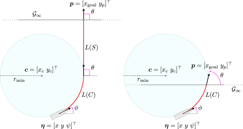
Figure 5: Diagram depicting the geometry of the Dubins path to an infinite line $\mathcal{G}_{\infty}$ for two possible cases.

Proof.

See Appendix A. ∎

IV-B2 Obstacles-only

The following is an admissible heuristic for $\eqref{eq:swath_cost}$, i.e., a lower bound for the collision cost of the swath $\mathcal{S}(\bm{\pi})$ given a pose $\bm{\eta}$ and the current goal $\mathcal{G}_{\text{int}}$. Let $w\in\mathbb{N}$ be the width of the ship footprint in costmap grid units. Now suppose that we have a path $\bm{\pi}$, starting from $\bm{\pi}(0)=\bm{\eta}$ and ending at $\bm{\pi}(L_{f})\in\mathcal{G}_{\text{int}}$, and a corresponding swath $\mathcal{S}(\bm{\pi})$ that sweeps rows $i$ through $j$ in the costmap for a total of $N=j-i+1$ rows. It must hold that the part of the swath that covers a particular row must consist of a set of grid cells $\mathcal{S}^{\prime}\subset\mathcal{S}(\bm{\pi})$ with at least $w$ consecutive elements, for all $N$ rows. In other words, we have $|\mathcal{S}^{\prime}|\geq w$ in the general case and $|\mathcal{S}^{\prime}|=w$ when the ship heading $\psi$ is aligned with the length of the channel / costmap. A lower bound for the cost of the single-row swath $\mathcal{S}^{\prime}$ for any particular row $k$ in the costmap is therefore achieved by selecting the lowest sum of $w$ consecutive grid cells in the $k$-th row. If we extend this to all $N$ rows in the costmap that make up the swath $\mathcal{S}(\bm{\pi})$, then we get a lower bound for the cost of the swath $\mathcal{S}(\bm{\pi})$ for all paths $\bm{\pi}$ from $\bm{\eta}$ to $\mathcal{G}_{\text{int}}$ and for all $\bm{\eta}$. This gives us an admissible heuristic function $h_{2}(\bm{\eta})$ for the total collision cost $C_{f}$ in $\eqref{eq:swath_cost}$. Although this heuristic relies on a loose lower bound on the cost, it is efficient to compute (linear search for each row) and admissibility is guaranteed.

V Optimization-Based Improvement Step

In the previous section, we described our proposed lattice-based planner to efficiently compute low-cost reference paths for a tracking controller. While the planner computes optimal solutions to the discretized planning problem defined by the graph $G^{\mathcal{P}}$, planned paths often contain excessive oscillations [57, 58], and the quality of the solution varies depending on how the lattice is initialized given the current pose of the ship $\bm{\eta}_{\textnormal{cur}}$. More broadly, the solutions are suboptimal for the following continuous path planning problem:

—l—[2] π, κ, L_f J = L_f + αC_f ˙x(s) = cos(ψ)   & s ∈[0, L_f] ˙y(s) = sin(ψ)   & s ∈[0, L_f] ˙ψ(s) = κ(s)   & s ∈[0, L_f] -r_min^-1 ≤κ(s) ≤r_min^-1   & s ∈[0, L_f] F(π(s)) ⊂I   & s ∈[0, L_f] π(0) = η_cur π(L_f) ∈G_int, where the constraints (V)-(V) are from the unicycle model (8) and the constraint (V) ensures the ship body (characterized by the footprint $\mathcal{F}$) remains within the ice channel. In this version of the problem, the total collision cost $C_{f}$ extends the function (10) to its continuous form, where we have an arc length parameterized line integral introduced in the next section. We will show how we can define a suitable differentiable function for the total collision cost that maintains the notions of ship footprint and swath using ideas from [59]. Similar to [56, 39, 43], we propose an optimization-based improvement step in a two-stage planning pipeline. In particular, we solve the path planning problem (V) in the continuous domain producing a locally optimal solution to refine the path computed by the lattice planner, which is used as an initial feasible solution to warm-start an optimization solver.

In the first step, we define a smooth function $c_{\text{obs}}(x,y)\geq 0$ representing a scalar field for the collision cost from the grid-based costmap generated by the original discrete collision cost in (9). We use bicubic interpolation to fit the costmap data to ensure that we have a smooth function for the collision cost everywhere in the environment. This includes the boundaries of the obstacles where there are clear discontinuities in the discrete costmap.

V-A Continuous Function for Total Collision Cost

With $c_{\text{obs}}(x,y)$ defined, we now need a way to calculate the total collision cost where there is a clear relationship with (10). We use the notion of body points from [59] which we define formally as follows:

Definition 1 (Body Points).

Let $\mathcal{B}\subset\mathbb{R}^{2}$ denote a set of body points where each body point $\bm{b}\in\mathcal{B}$ is a position $(x_{\mathcal{B}},y_{\mathcal{B}})$ in the body-fixed coordinate frame (see Section II-A).

Consider the path of a particular body point $\bm{b}$ given a path $\bm{\pi}$. This gives the arc length parameterized curve $\bm{\pi}_{\bm{b}}=\{\bm{g}(\bm{\pi}(s),\bm{b}):s\in[0,L_{f}]\},$ where the affine function $\bm{g}:\mathcal{C}\times\mathcal{B}\rightarrow\mathbb{R}^{2}$ maps a pose $\bm{\eta}$ and a body point $\bm{b}$ to the corresponding position in the world coordinate frame:

$$\bm{g}(\bm{\eta},\bm{b})=\begin{bmatrix}\cos(\psi)&-\sin(\psi)\\ \sin(\psi)&\cos(\psi)\end{bmatrix}\bm{b}+\begin{bmatrix}x\\ y\end{bmatrix}.$$ (23)

Next, consider the cost that the body point $\bm{b}$ collects in the cost field $c_{\text{obs}}(x,y)$ given by the line integral along the path $\bm{\pi}_{\bm{b}}$. We can therefore define the total collision cost $C_{f}$ as the cost of each of the body point paths integrated over all the body points:

$$C_{f}=\int_{0}^{L_{f}}\int_{\mathcal{B}}c_{\text{obs}}(\bm{g}(\bm{\pi}(s),\bm{b})))\left\lVert\frac{d}{ds}\bm{g}(\bm{\pi}(s),\bm{b}))\right\rVert d\bm{b}\ ds.$$ (24)

The operator $||\cdot||$ denotes the Euclidean norm of the vector $d\bm{g}/ds$, i.e., the arc length derivative of $\bm{g}$, which we can immediately get by looking at $\eqref{eq:definition_g}$ and recalling the unicycle model in the constraints (V)-(V):

$$\frac{d}{ds}\bm{g}(\bm{\eta},\bm{b})=\begin{bmatrix}-\kappa\sin(\psi)&-\kappa\cos(\psi)\\ \kappa\cos(\psi)&-\kappa\sin(\psi)\end{bmatrix}\bm{b}+\begin{bmatrix}\cos(\psi)\\ \sin(\psi)\end{bmatrix}.$$ (25)

Note that in (25), we have suppressed the arc length parameter $s$ on the right-hand side of the equation; hence, $\kappa$ and $\psi$ should be interpreted as $\kappa(s)$ and $\psi(s)$, respectively. Multiplying the cost $c_{\text{obs}}$ by $\lVert d\bm{g}/ds\rVert$ ensures that we are integrating along the particular path $\bm{\pi}_{\bm{b}}$ for each body point $\bm{b}\in\mathcal{B}$, and not the path $\bm{\pi}$ unless $\bm{b}=[0\ 0]^{\top}$.

V-B Comparison with Body Points in Zucker et al.

The total collision cost $C_{f}$ in $\eqref{eq:optim_step_total_collision_cost}$ shares similarities with the obstacle objective in the collision-free trajectory optimization approach from [59]. However, in addition to optimizing a collision-prone path rather than a collision-free trajectory, our cost function $c_{\text{obs}}$ does not assign costs in the obstacle-free region $\mathcal{W}_{\text{free}}$ given $\mathcal{W}_{\text{obs}}$ in contrast to the obstacle objective in [59]. This means that we need to define the body points slightly differently.

To see why this is the case, consider the simple scenario illustrated in Fig. 6. It consists of an ice floe $\mathcal{O}$ and two candidate straight paths $\bm{\pi}^{(1)}$, $\bm{\pi}^{(2)}$, both of which result in a collision with $\mathcal{O}$ where $\bm{\pi}^{(1)}$ results in a more head-on collision than $\bm{\pi}^{(2)}$. Now suppose that the set of body points $\mathcal{B}$ is defined along the exterior of the body as in [59]. In particular, consider the following two subsets of $\mathcal{B}$: $\{\bm{b}_{1}$, $\bm{b}_{2}$} located at the stern and bow, respectively, and $\{\bm{b}_{1}^{\prime}$, $\bm{b}_{2}^{\prime},\dots,\bm{b}_{j}^{\prime}\}$ positioned along one of the straight sides of the ship body. We want to compare the total collision cost $C_{f}$ from (24) for the two paths by examining how $\mathcal{B}$ affects this cost. Observe that for path $\bm{\pi}^{(2)}$ each body point in $\{\bm{b}_{1}^{\prime}$, $\bm{b}_{2}^{\prime},\dots,\bm{b}_{j}^{\prime}\}$ accumulates a cost from the region in the cost field highlighted in magenta. By comparison, consider how this cost field region affects the cost of $\bm{\pi}^{(1)}$. Here, there are exactly two body points, $\bm{b}_{1}$ and $\bm{b}_{2}$, which accumulate cost in this region. This suggests that the cost computed from (24) will be higher for $\bm{\pi}^{(2)}$ compared to $\bm{\pi}^{(1)}$. However, if we recall the original swath cost formulation for $C_{f}$ in (10), we know that $\bm{\pi}^{(1)}$ should be assigned a higher cost between these two candidate paths.

As a result, from the example shown in Fig. 6, defining body points exclusively on the outline of the ship body leads to cases where certain subsets of $\mathcal{B}$ disproportionately accumulate cost from our cost field. This example also illustrates that such a $\mathcal{B}$ would create an incentive to reduce the cost of a path by slightly adjusting it such that the interior region of the ship body now passes through a high-cost region that was part of the original path.

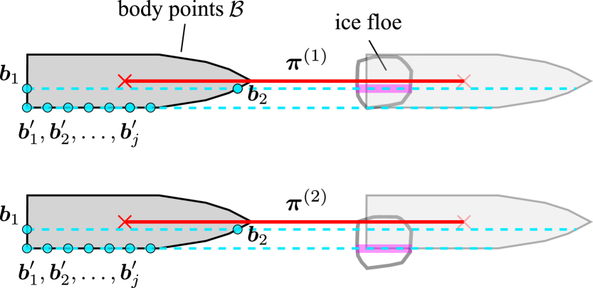
Figure 6: A simple scenario to illustrate the problem with defining body points exclusively on the outline of the ship body. Two candidate paths are considered, $\bm{\pi}^{(1)}$ and $\bm{\pi}^{(2)}$, in the top and bottom parts of the figure, respectively. We examine the cost of these two paths by considering the contribution to the cost from two subsets of $\mathcal{B}$: $\{\bm{b}_{1},\bm{b}_{2}\}$ and $\{\bm{b}_{1}^{\prime},\bm{b}_{2}^{\prime},\dots,\bm{b}_{j}^{\prime}\}$, depicted as cyan dots. The corresponding paths of the body points are shown with the cyan dotted lines. We see that in the bottom scenario, the magenta region of the cost field is disproportionately penalized from $\{\bm{b}_{1}^{\prime},\bm{b}_{2}^{\prime},\dots,\bm{b}_{j}^{\prime}\}$ compared to the top scenario.

V-C Options for an Appropriate Set of Body Points

To address the problems discussed above with regard to defining body points, we present three possible options to define $\mathcal{B}$ and show an example for each in Fig. 7:

1. Let $\mathcal{B}$ be equal to the ship footprint $\mathcal{F}(\bm{\eta})$ at $\bm{\eta}=[0\ 0\ 0]^{\top}$ (Fig. 7 (top)).

2. Let $\mathcal{B}$ be the set of points inside the rectangle that encloses $\mathcal{F}(\bm{\eta})$ at $\bm{\eta}=[0\ 0\ 0]^{\top}$ (Fig. 7 (middle)).

3. Let $\mathcal{B}$ be the set of points along a straight line that is perpendicular to $\psi$, has a length equal to the width of the ship, and is positioned at the tip of the bow (Fig. 7 (bottom)).

Remark 2 (Comparison with the Swath).

Consider how the set of body point paths from each of the three options for defining $\mathcal{B}$ compares to the swath $\mathcal{S}(\bm{\pi})$ given a path $\bm{\pi}$. Option (i) ensures no region from the swath is missed, option (ii) over-approximates the swath during turns, while option (iii) results in an under-approximation (albeit at a lower computational cost).

Remark 3 (Weighting Body Points).

To enable fine-tuning of planning behavior, such as preferring collisions with areas of the hull that are reinforced, we can define a set of weights. Let each body point $\bm{b}\in\mathcal{B}$ be assigned a weight $w\geq 0$ representing the relative penalty for accumulating cost.

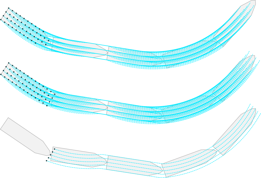
Figure 7: Three possible options to define the set $\mathcal{B}$. The dots are body points sampled from the respective $\mathcal{B}$ and the cyan dotted lines are the sampled body point paths.

V-D Transcription and Solver

The continuous planning problem in (V), incorporated with the collision cost $C_{f}$ from (24), is solved numerically using tools from optimal control. In particular, we transform the continuous problem into a discrete nonlinear program (NLP) using direct multiple shooting. The path is discretized into $N+1$ decision variables $\bm{\eta}_{1},\dots,\bm{\eta}_{N+1}$ and $N$ decision variables $\kappa_{1},\dots,\kappa_{N}$ for the curvature $\kappa$ (i.e. the signal that controls $\dot{\psi}$). Each control interval occurs over an arc length step of $\Delta s$, analogous to a time step in trajectory optimization. To avoid large changes in curvature over a small distance, we add a smoothness term to the objective function with a weight parameter $\lambda\geq 0$. Integration of the ODE for the unicycle model is performed using the 4th-order Runge-Kutta method (RK4).

We define a finite set $\mathcal{B}_{d}$ of discrete body points uniformly spaced on a square grid with spacing $\Delta b$, covering the rectangle that encloses the ship body (i.e., option (ii) discussed in the previous section). Each body point $\bm{b}_{j}\in\mathcal{B}_{d}$ has a corresponding weight $w_{j}>0$. Let $\ell$ denote the length of the ship body and recall that $\Delta_{\text{grid}}$ is the resolution of the discrete costmap. By default, each weight $w_{j}$ is assigned a constant value of

$$w_{j}=\frac{\alpha\Delta b^{2}}{\ell\Delta_{\text{grid}}^{2}},$$ (26)

such that the terms in the objective—path length $L_{f}$ and total collision cost $C_{f}$—in the optimization problem have the same scaling as in the lattice planning stage. This expression is determined by calculating the average number of times a grid cell $\bm{k}\in\mathbb{N}$ in the original discrete costmap is covered by a body point $\bm{b}_{j}\in\mathcal{B}_{d}$ along a path $\{\bm{\eta}_{i}\}_{i=1}^{N+1}$ with an arc length step of $\Delta s$. Suppose we have a straight path (i.e. $\kappa_{i}=0$ for $i=1,\dots,N$) where $\ell$, $\Delta s$, and $\Delta b$ are all multiples of $\Delta_{\text{grid}}$. A subset of this path is shown in Fig. 8. In this example, it is easy to see the two important ratios, namely $\Delta s/\ell$ and $\Delta b^{2}/\Delta_{\text{grid}}^{2}$ which control how often a grid cell is sampled on average. These two ratios, along with the weight $\alpha$ from (V), give (26) ($\Delta s$ is missing here since it appears in the objective function described next).

We remove the constraint $\eqref{eq:constraint5}$ in the original optimization problem by assigning a sufficiently high cost in the cost field for points in $\mathbb{R}^{2}$ outside the boundaries of the ice channel $\mathcal{I}$. The following is the resulting discrete optimization problem:

—l—[2] η_1,…,η_N+1,κ_1,…,κ_N, Δs ∑_i=1^N+1∑_b_j ∈B_d w_j c_obs(g(η_i, b_j)) ∥ddsg(η_i, b_j)∥Δs + L_f + λ∑_i=1^N(κi+1- κiΔs)^2 η_i+1 = f_RK4(η_i, κ_i, Δs)  & i = 1,…,N -r_min^-1 ≤κ_i ≤r_min^-1  & i = 1,…,N (x_i, y_i) ∈I  & i = 1,…,N η_1 = η_cur η_N+1 ∈G_int,

This problem is solved using the NLP solver, IPOPT [60] (interfaced with CasADi [61] in our experiments), and warmed started with the initial plan computed by the lattice planner stage by resampling the path to $N+1$ points.

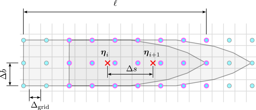
Figure 8: Illustration of the components involved to derive (26). The square grid shows the discrete costmap with resolution $\Delta_{\text{grid}}$. Body points are shown for two consecutive poses, $\bm{\eta}_{i},\bm{\eta}_{i+1}$, where the points outlined in magenta are overlapping. For the sake of visualization, everything here is nicely aligned with the costmap grid.

VI Simulation Results

Extensive simulation experiments were performed to evaluate our framework’s ability to autonomously navigate a vessel in broken ice fields. The particular scenario considered is a platform supply vessel (PSV) navigating through broken ice fields of various ice concentrations and containing variable-sized medium thick first-year ice floes. We considered a narrow channel of size 1000 m $\times$ 200 m (L$\times$W) with four possible ice concentrations: 20%, 30%, 40%, and 50%. For each concentration, we generated 100 different ice fields where for each ice field we performed three trials: two baselines and the proposed method. At the start of each trial, the vessel was positioned 100 m before the beginning of the ice field, aligned with the channel length, and centered with respect to the channel width (see Fig. 9). A trial ended when the vessel reached the end of the ice field, a distance of 1100 m from the starting position. A standard PC with an Intel Core i7-7700K processor with 32 GB of memory was used for these experiments. The total wall clock time to run all simulation tests and evaluation scripts was 60 hours (not including the time to render animations). In the next sections, we describe our experimental setup in more detail, including our open-source physics simulator, followed by the simulation results. Additional details regarding the experimental setup, including the PSV model shown in Fig. 10 and the controller, are provided in Appendix B.

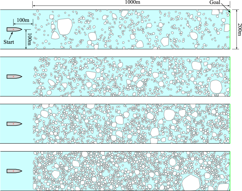
Figure 9: Sample ice fields generated for the simulation experiments. Four different ice field concentrations are shown: 20%, 30%, 40%, and 50% (top to bottom).

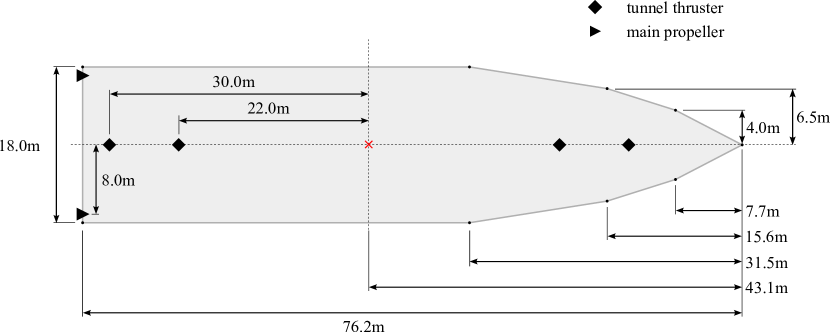
Figure 10: The dimensions, bow geometry, and actuator configuration of the vessel considered in the simulation experiments. The origin of the vessel is depicted by the red ‘x’.

VI-A Physics Simulator

Although there exist numerous works on numerical simulation of ship interactions with broken ice, e.g. [62, 20, 63, 64, 8, 53, 15, 19], none provide open source code and few are sufficiently efficient to perform extensive experiments. We therefore developed our own simulation solution.

Our simulator is built on top of the Python library Pymunk [65], which is a wrapper for the 2D real-time rigid body impulse-based physics engine Chipmunk2D [66]. Collisions between bodies are therefore treated as rigid-body inelastic collisions. This means that we ignore more complex scenarios, including ice-splitting. Similar approximations have been made in other models [20, 62]. We used existing simulation work from [62, 20, 67, 63, 64] and field data [68] to set the majority of the simulator parameters. A summary of these parameters along with the respective sources is provided in Table III in Appendix B.

We model the hydrodynamic force acting on the ice floes as a quadratic drag force [8],

$$\bm{F_{d}}=-\frac{1}{2}\rho_{w}C_{d}A_{proj}\bm{v}\|\bm{v}\|,$$ (27)

acting in the opposite direction of the ice floe linear velocity, $\bm{v}\in\mathbb{R}^{2}$. The values for the water density $\rho_{w}$ and the drag coefficient $C_{d}$ are from [64] and [63], respectively. The factor $A_{proj}$ is the projection of the submerged area of the ice floe along the direction of $\bm{v}$. However, since our simulation is in 2D, we assume that the submerged portion of each ice floe is proportional to the density ratio $\rho_{ice}/\rho_{w}$Regarding the drag torque, we model the effect on the angular velocity as an exponential decay.

The physics engine only handles the kinematics of the ship and therefore let the vessel dynamics account for the ice resistance forces. We do this by computing a generalized force vector $\bm{\tau}_{\text{env}}=[X_{\text{env}},Y_{\text{env}},N_{\text{env}}]^{\top}\in\mathbb{R}^{3}$ for a force $X_{\text{env}}$ in surge, force $Y_{\text{env}}$ in sway, and torque $N_{\text{env}}$ in yaw. This gives the net force and net torque experienced by the ship obtained by aggregating all impact forces and their corresponding contact points on the ship hull, logged during the current control interval. In practice, other environmental forces may be present in $\bm{\tau}_{\text{env}}$ such as wind and wave induced forces [10], but we ignore these additional disturbances here. Although we did not validate our simulator with real-world data, we observed a reasonable level of consistency in our simulation trials with data reported in [20, 19].

VI-B Metrics

The following information was stored for each simulated ship-ice collision: ice mass, collision impulse, kinetic energy loss in the system $\Delta K_{\text{sys}}$, change in kinetic energy of the ice $\Delta K_{\text{ice}}$, and contact points on the 2D ship hull. Using the logged collision data from a given trial, we computed the mean mass of the collided ice floes, the maximum magnitude of the impact force, the mean magnitude of the impact force, and the total kinetic energy loss of the ship, $\Delta K_{\text{ship}}$, using (15). We approximated the impact force as the collision impulse divided by the simulation time step [69].

The other two metrics of interest are the total energy consumption of the ship and the total transit time. Given the simulated velocities $\{\bm{\nu}_{k}\}_{k=1}^{N}$ and forces $\{\bm{\tau}_{k}\}_{k=1}^{N}$ for control steps $1,...,N$, we computed the total energy, $E$, as

$$E=\Delta t_{\text{ctrl}}\sum_{k=1}^{N}|\bm{\nu}_{k}|^{\top}\cdot|\bm{\tau}_{k}|,$$ (28)

where $|\cdot|$ denotes the element-wise absolute value operator. These additional metrics offer insight into the trade-off between efficiently traversing the ice field and altering course to avoid significant impacts with ice.

VI-C Baselines

We considered two baseline methods, referred to as Straight and Skeleton. The former plans a straight path from the initial position of the ship to the goal, while the latter refers to the shortest open water path routing approach described in [33, 12]. In the first step, the Skeleton method generates a morphological skeleton image [70] of the open water area $\mathcal{W}_{\text{free}}$. This provides a useful representation of the environment’s topology from which a graph can be constructed and then searched, producing a path. The path is then post-processed with a smoothing operation, which accounts for the minimum turning radius $r_{\min}$ of the ship. We also added logic that progressively erodes the original occupancy image of the ice field until an open water path is found since no path may exist in the original image for high concentration ice fields. For a fair comparison with AUTO-IceNav, we configured the same replanning strategy outlined in Algorithm 1 for the two baselines. The parameter settings for AUTO-IceNav, including our calibration process for the parameter $\alpha$ such that (7) gives a good approximation of the true navigation cost, are given in Appendix C-A. Note that the nominal speed $U_{\text{nom}}$ was set at a constant 2 m/s to facilitate the analysis across trials with different ice concentrations.

VI-D Results

Concentration	Method	Mean collided ice mass	Max impact force	Mean impact force	Ship KE loss $\Delta K_{\text{ship}}$	Total Energy $E$	Total time
		($10^{3}$ kg)	($10^{3}$ kN)	(kN)	($10^{3}$ kJ)	($10^{3}$ kJ)	(s)
20%	Straight	360	1025	576	100	245	604
	Skeleton	224	461	252	37	233	620
	AUTO-IceNav	99	134	133	22	218	615
30%	Straight	196	960	383	125	273	604
	Skeleton	133	447	205	82	259	618
	AUTO-IceNav	82	147	140	41	236	614
40%	Straight	168	936	394	147	316	613
	Skeleton	107	392	200	102	296	620
	AUTO-IceNav	78	156	165	63	281	618
50%	Straight	137	786	362	167	335	609
	Skeleton	99	360	235	128	363	638
	AUTO-IceNav	74	160	210	93	335	621

TABLE I: Results from the simulation experiments. Scores are averaged over 100 trials for a given ice concentration and navigation method.

A total of 1200 trials were conducted: 4 concentrations $\times$ 3 navigation strategies $\times$ 100 ice fields. The trials spanned 206 hours of simulation time logging 37 million ship-ice collisions across 1320 kilometers of ship transit. We present a summary of the results in Table I. The scores for each metric in the table are averaged over the 100 trials performed for a particular ice concentration and navigation method. In the AUTO-IceNav trials, the ship collided with smaller ice floes on average and experienced fewer head-on collisions, resulting in a significant decrease in the mean and maximum impact forces generated by the ship-ice collisions. Compared to the Straight and Skeleton trials, we reduced the mean impact force by 62% and 27%, respectively, and the maximum impact force by 84% and 64%, respectively. These improvements are best visualized in Fig. 11, where the force vectors are plotted at their respective contact points for all collisions recorded between the three methods. Observe the significant differences in the spatial distribution of large impacts across the ship hull and the magnitude of the force vectors between AUTO-IceNav and the two baselines. Further, observe that the Skeleton method consistently outperformed Straight, suggesting that the curved open-water paths were partially successful in avoiding collisions and head-on impacts.

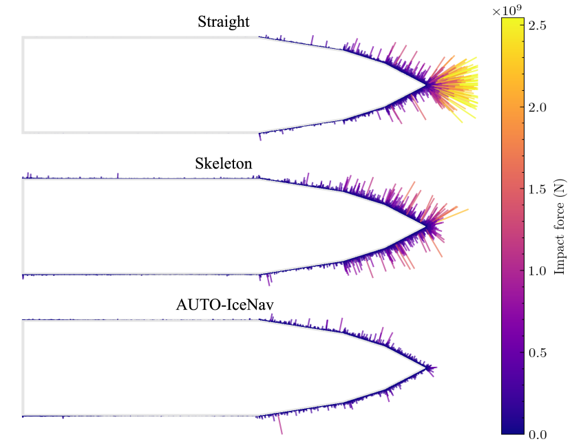
Figure 11: Visualization of all impact forces and the corresponding contact-points from the ship-ice collisions that occurred during the simulation trials. Each vector depicts the direction and relative magnitude of the impact force experienced by the ship’s hull (grey outline). In total, the Straight, Skeleton, and AUTO-IceNav trials logged 11.3 million, 13.0 million, and 12.3 million collisions, respectively.

In addition to the reductions in impact forces, which decrease the potential for damage to the vessel, our experiments also demonstrated improvements in energy use with our proposed method. The smaller impact forces resulted in a decrease in the total kinetic energy loss of the ship from colliding with ice floes. Summing $\Delta K_{\text{ship}}$ across trials, AUTO-IceNav resulted in a 59% reduction in the ship’s kinetic energy loss compared to the Straight trials. This efficiency gain more than offset the additional energy required to follow the 2% longer paths generated by AUTO-IceNav. In particular, our method achieved a decrease of 8.5% in total energy use $E$ compared to the Straight trials. This suggests that the weighted sum of the path length and the proposed total collision cost is effective in capturing the true navigation cost of transiting a broken ice field. The guidelines established by the Canadian Coast Guard for ice navigation advise vessels to extend their journey as necessary to reduce the risk of damage which, in certain scenarios, can lead to voyages with less fuel consumption [7]. In simulation, our results clearly demonstrated the feasibility of achieving both of these objectives with an autonomous navigation system. Naturally, we should also be considering the additional cost associated with longer travel time, however, this cost is likely negligible compared to the possible cost incurred from damaging the ship. Across 400 trials, totaling 67.5 hours of ship transit, AUTO-IceNav increased total travel time by just 1.5 hours compared to straight navigation, representing only a 2% increase. It is also worth noting that the controller performed adequately in tracking the reference path at the target speed. The average cross-track error was 2.0 m, while the average heading error was 1 degree.

VI-E Evaluating the Optimization Stage

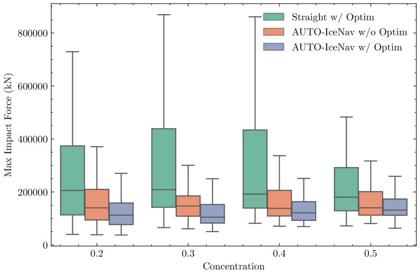
Figure 12: Results from evaluating our proposed optimization stage. Each box in the boxplot represents the distribution of maximum impact forces across 100 trials for a given ice concentration and navigation method.

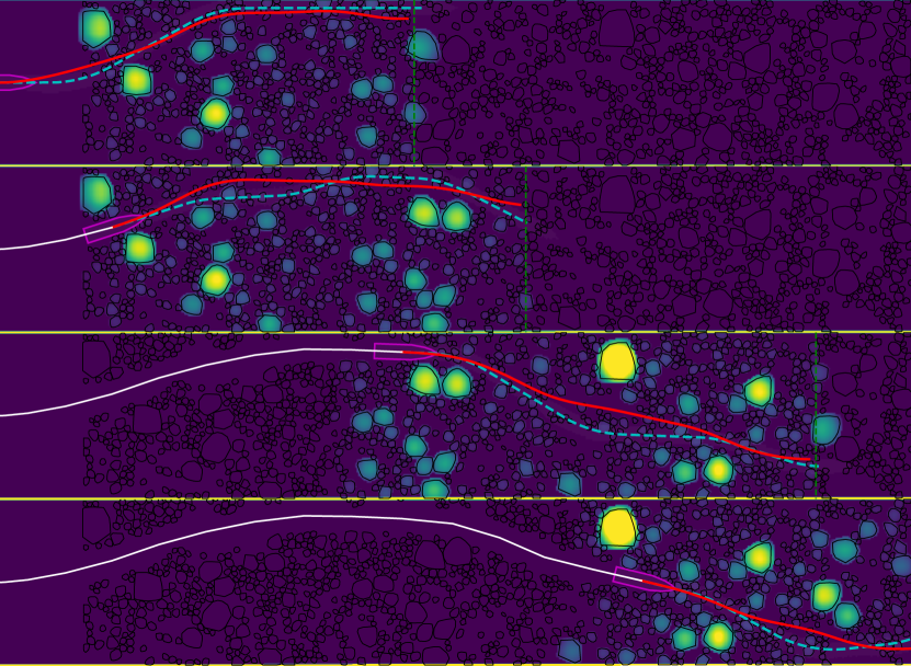
Figure 13: Four snapshots taken from a sample simulation trial in a 40% concentration ice field using our proposed method. The initial path computed in the lattice planning stage (cyan dotted line) and the optimized path (red line) are overlaid on the costmap. Visually, we see that the red path tends to be better in terms of both the path length and the ship-ice collisions that occur along it. The actual path of the ship is displayed in white and the green dotted line shows the intermediate goal $\mathcal{G}_{\text{int}}$.

In addition to testing our method against the Straight and Skeleton baselines, we evaluated the effectiveness of our proposed optimization-based improvement step. We conducted the same 400 trials described above for our method without the second stage. From these additional trials, we see that the optimization stage provides a clear improvement in navigation performance. On average, the second stage reduced the maximum and mean impact forces by 19% and 10%, respectively, while using 1% less total energy compared to the AUTO-IceNav trials without optimization. As another baseline, we conducted 400 trials with the optimization stage warm-started with a straight path. These trials demonstrate that, while the optimization stage yields significant improvements, the solutions remain locally optimal. We therefore achieved better performance when the optimization stage was warm started with the lattice planning solution. Fig. 12 shows the results for the maximum impact force and Fig. 13 shows four representative snapshots of a sample AUTO-IceNav trial in a 40% concentration ice field.

VII Results from Physical Testbed

In addition to the experiments performed in simulation, we conducted real-world experiments at model-scale in the Offshore Engineering Basin (OEB) research facility in St. John’s, Newfoundland and Labrador. The NRC-managed facility features a large basin measuring 75 m $\times$ 32 m, shown in Fig. 14. Our experimental setup closely followed the setup described in our preliminary work [21] with some necessary adjustments. In contrast to the NRC ice tank used in our previous experiments, the OEB is a room temperature facility. As a result, we used a collection of plastic polygon pieces cut from polypropylene sheets (density 991 kg / m³ and thickness 0.012 m) commonly used for artificial ice floes [6]. In total, we had around 300 polygons which provided an ice concentration of 30$\%$ over a net-confined area of 20 m $\times$ 6 m (L$\times$W) for the ice channel.

The ship model used in these experiments was a 1:45 scale platform supply vessel (PSV), designed with a typical hull shape and constructed by the NRC. The dimensions of the vessel are 1.84 m $\times$ 0.38 m $\times$ 0.43 m (L$\times$W$\times$H) and weighs 90 kg. For propulsion, the PSV contains two tunnel thrusters (fore and aft) and two main propellers. More details on the PSV are described in [12]. To control the vessel, we employed a Dynamic Positioning (DP) controller similar to the one used for the simulation experiments (see Appendix B-B). The forward thrust was set constant, which achieved a nominal speed of 0.2 m/s. To capture ice information, we used a ceiling-mounted camera pointing down on the basin and used a similar image segmentation pipeline (updated at 30 Hz) described in [33]. An optical-based motion capture system (Qualisys) provided 3D (i.e. 6 DoF) state information of the vessel at 50 Hz.

We performed a total of 60 trials and used the same baselines, i.e. Straight and Skeleton, from our simulation experiments to compare against our approach. Before starting each trial, the PSV was manually positioned along a starting line, with its heading aligned with the channel length. We considered three general starting positions along the starting line relative to the channel width: center, right, and left. For each navigation strategy, we performed 20 trials, initializing 6 of them with a center start, 7 with a left start, and 7 with a right start. The goal line was established at the opposite end of the channel, located 16 m from the starting point.A diagram of the experimental setup is shown in Fig. 15. Note that we used a random ordering to conduct the 60 trials.

Figure 14: Side view of the experimental setup in the Offshore Engineering Basin research facility. The ice basin contains a collection of plastic ice pieces cut from sheets of polypropylene.

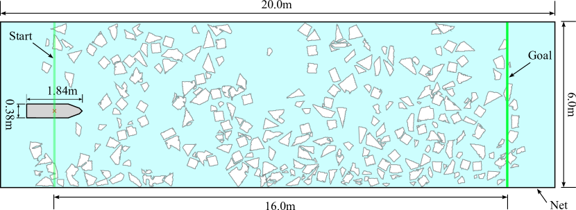
Figure 15: Diagram showing the dimensions of the model-scale ship and ice channel for our physical testbed.

VII-A Metrics

The small-scale setup limited our ability to rely on several of the metrics discussed in the simulation section, including impact forces derived from acceleration data measured by the onboard IMU. We computed an approximation for $\Delta K_{\text{ship}}$ by performing object tracking on the ice segmentation data. A segmented ice floe is represented as a polygon, defined by a sequence of vertices at time $t_{k}$, where $k\in{1,\dots,N}$ denotes the time steps of the trial. Each polygon was tracked using a Kalman filter to estimate the position $\bm{p}\in\mathbb{R}^{2}$ and the velocity $\bm{v}\in\mathbb{R}^{2}$ of the polygon’s centroid. Using the velocity estimates, we identified the subset of segmented ice floes, $\mathcal{Q}$, that were likely pushed by the ship during a particular trial. This included scenarios where an ice floe was in direct contact with the ship or was touching a chain of other ice floes that were all being pushed by the ship. From here, we computed several approximations for the work done on the ice by the ship, which is an equivalent definition of $\Delta K_{\text{ice}}$ when the ice floes are rigid bodies. This provides a reasonable way to compute $\Delta K_{\text{ship}}$ using (15) where we treat $\Delta K_{\text{sys}}$ as negligible.

The work $W$ of a net force $\bm{F}$ applied to a particle with mass $m$ is given by

$$W=\int_{t_{1}}^{t_{2}}\bm{F}\cdot\bm{v}dt=m\int_{t_{1}}^{t_{2}}\bm{a}\cdot\bm{v}dt,$$ (29)

where $\bm{a}$, $\bm{v}$ is the particle’s acceleration and velocity, respectively. We considered the net force acting on the ice floes to consist of the drag force and the force from the ship (either via direct contact or from a chain of ice floes). This means that in the absence of a ship force, work done on the ice will be negative if the ice floe speed $\|\bm{v}\|$ is nonzero. We can thus approximate the work done by the ship on the ice by only considering the instances of positive work in the object tracking data. We used the velocity estimates $\{\bm{v}^{P}_{k}\}_{k=1}^{N}$ for each pushed ice floe $P\in\mathcal{Q}$ tracked by the Kalman filter to give us the total positive work,

$$W_{1}=\sum_{P\in\mathcal{Q}}m^{P}\sum_{k=1}^{N-1}(t_{k+1}-t_{k})\max(0,\bm{a}^{P}_{k}\cdot\bm{v}^{P}_{k}).$$ (30)

Note, the ice mass $m^{P}$ is computed as the product of ice thickness, ice density, and area. Acceleration $\bm{a}_{k}^{P}\in\mathbb{R}^{2}$ was approximated via finite differencing of the velocity estimates. If we ignore the work associated from a resultant torque, then (30) gives a good approximation for the positive work done by the resultant force applied on a rigid body.

We wanted to see whether a coarser metric (i.e., worse approximation but perhaps less prone to noise) for work would produce similar results as (30). Hence, instead of considering an accumulation of positive work, we considered the change in kinetic energy for each polygon $P\in\mathcal{Q}$ given the maximum speed attained $v^{P}_{\max}=\max{\{\|{\bm{v}}_{k}^{P}\|\}_{k=1}^{N}}$ and the initial speed $\|\bm{v}_{1}^{P}\|$. Using the work-energy principle, we get our second metric $W_{2}$ for the work done by the ship on the ice:

$$W_{2}=\frac{1}{2}\sum_{P\in\mathcal{Q}}m^{P}((v^{P}_{\max})^{2}-\|\bm{v}_{1}^{P}\|^{2}).$$ (31)

Observe that (31) does not capture the scenario where an ice floe was pushed on several distinct occasions by the ship meaning $W_{1}\geq W_{2}$. As a second coarse metric for work, we computed the product of the ice mass $m^{P}$ and the arc length $s^{P}$ of the path $\{\bm{p}^{P}_{k}\}_{k=1}^{N}$ taken by the polygon $P\in\mathcal{Q}$:

$$W_{3}=\sum_{P\in\mathcal{Q}}m^{P}s^{P}.$$ (32)

While (32) lacks a direct connection to work, it offers a straightforward way for capturing the amount by which the ship changed the ice environment.

Other metrics we computed from the object tracking data are the number of pushed ice floes given by the cardinality of the set $\mathcal{Q}$ and the mean mass of the set of ice floes that collided with the ship. The latter metric was computed by finding the subset of polygons $\mathcal{Q^{\prime}}\subseteq\mathcal{Q}$ that intersected the ship footprint at some point during the trial. We also included the total time to transit the ice channel.

VII-B Results

Difficulty	Method	Mean collided ice mass (kg)	No. pushed ice	$W_{1}$ (J)	$W_{2}$ (J)	$W_{3}$	Total time (s)
Easy	Straight	1.28	44.13	0.28	0.20	40.91	91.39
	Skeleton	1.21	128.00	0.75	0.47	127.11	115.27
	AUTO-IceNav	1.15	35.00	0.20	0.15	28.87	101.91
Medium	Straight	1.27	68.40	0.44	0.31	65.72	89.52
	Skeleton	1.31	102.63	0.59	0.38	106.55	110.06
	AUTO-IceNav	1.17	38.00	0.21	0.13	28.60	102.90
Hard	Straight	1.22	109.14	0.85	0.52	144.69	97.15
	Skeleton	1.24	97.11	0.64	0.41	109.82	110.73
	AUTO-IceNav	1.20	49.33	0.33	0.21	53.86	109.35

TABLE II: Results from experiments done in the physical testbed.

We present a summary of the results in Table II and show several snapshots of a sample AUTO-IceNav trial in Fig. 17. The table shows the metrics discussed in Section VII-A, where the scores are averaged across trials for each navigation method and difficulty level. The three levels, ‘easy’, ‘medium’, and ‘hard’, are based on the average subjective difficulty scores assigned to each trial by the authors as part of a blind evaluation process (see Appendix D for more details).

In terms of work, our approach outperformed the baselines in the three difficulty levels. Compared to the second-best score for $W_{1}$ from (30), we achieved improvements of $29\%$, $52\%$, and $48\%$ for the easy, medium, and hard tests, respectively. These relative improvements are similar across the other two work metrics, suggesting that even the coarser metric $W_{3}$ provides a useful measure of performance. Fig. 16 provides a complete picture of the results for $W_{1}$. Observe that for the easy trials, our method provided the smallest gains over navigating straight through the ice field. This gap between Straight and AUTO-IceNav grows as the trials become more difficult. In addition, Straight is outperformed by both AUTO-IceNav and Skeleton for the hard trials. Interestingly, the Skeleton approach exhibits similar performance across difficulty levels and performed worse on average for the easy trials. However, it is difficult to draw definitive conclusions due to the limited number (only 3) of easy Skeleton trials. The results also indicate that AUTO-IceNav enabled the ship to, on average, collide with smaller ice floes and interact with fewer polygons.

We highlight several limitations of these experiments. Due to resource constraints, we were unable to perform trials with varying ice concentrations like we did in the simulation experiments. It would be interesting to see how our improvements over the baselines compare for higher concentration ice fields, e.g. 40% and 50% ice concentration. We hypothesize that such experiments would show similar performance trends compared to the simulation results described in Section VI-D. However, in contrast to the simulation experiments, the plastic ice floes had a narrower range in size and shape, which may have limited the range of possible scenarios encountered during ship transit. At a broader level, the small-scale experiment setup and relatively lightweight fake ice made it challenging to simulate full-scale behavior. For instance, the acceleration measurements from the onboard IMU were not particularly meaningful, as mentioned earlier. We were also unable to make meaningful comparisons in total energy consumption due to the lack of resistance provided by the fake ice. This means that the computed work scores seem less significant if we compare them with the total energy used by the ship actuators. Future experiments in the physical testbed would, therefore, benefit from an increase in the ice concentration and the ice floe thickness.

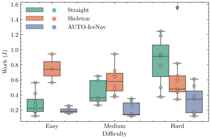
Figure 16: Total work done on the ice compared across method and difficulty level. Work was computed using the object tracking data and (30).

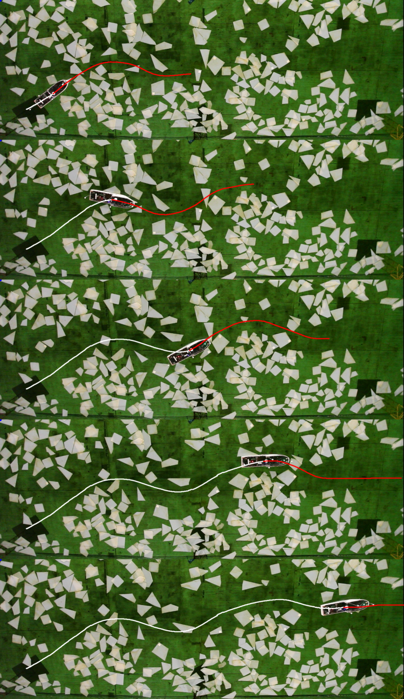
Figure 17: Five snapshots from a sample AUTO-IceNav trial, displaying the planned path in red and the actual ship path in white. Videos of trials can be found at https://github.com/rdesc/AUTO-IceNav#demo-videos-from-nrc-experiments.

VIII Conclusion and Future Work

In this work, we examined the problem of local navigation for autonomous ships operating in broken ice fields. We presented our framework, AUTO-IceNav, which we showed to be an effective navigation strategy both in simulation and in a physical testbed. Our results demonstrated significant reductions in the mean and maximum impact forces from ship-ice collisions and decreased energy consumption compared to naive navigation strategies such as navigating straight. We highlight several key areas where our approach may be improved.

A major direction for future work is to account for the changing ice field during the planning stage. This means that instead of relying on frequent replanning, we use a prediction model of the ice field to better inform planning behavior. The motion of ice floes is influenced both by the actions taken by the ship and by environmental disturbances [43]. This suggests that a useful ice prediction model should receive as input information that encodes how the ship will navigate the current environment. Modeling the relationship between the state of the ice field, the action of the ship, and the navigation cost may be a suitable problem for reinforcement learning (RL) methods or other learning-based approaches.

Improving the cost function for the total collision cost is another significant direction for future work. Higher-fidelity models for ship-ice collisions are described in [55, 71, 20], which account for additional important features that affect the collision physics, including the angles of the ship’s hull and the shapes of the ice edges [55]. However, such models do not translate well with our current costmap-based approach and, therefore, would require novel solutions for designing a suitable cost function for efficient planning. Even more challenging would be to account for the cost associated with the ship breaking through the ice, which typically occurs in head-on collisions with larger ice floes [15]. Another improvement would be to add constraints on the maximum impact force experienced during ship-ice collisions, as it has a greater effect on structural safety than overall energy [15].

As we observed in the physical experiments, the ice segmentation pipeline is prone to producing noisy outputs, affecting downstream processing. This suggests the use of a probabilistic representation of the ice field where measurements are used to iteratively update beliefs on the shape, position, and orientation of the ice floes. Such a probabilistic approach would be particularly useful in accounting for uncertainties inherent in ship-mounted sensors used to capture ice fields and other potential hazards present in ice navigation [18].

Finally, another major improvement to our method would be to treat the ship’s velocity as variable rather than keeping it constant when calculating the total travel time and total collision cost. Such an approach would likely result in substantial performance gains in terms of navigation metrics and could enable a wider range of desirable ship maneuvers for ice navigation, including slowing down before large collisions, as necessary.

Appendix A Proof of Theorem 1

Consider a circle of minimum turning radius $r_{\min}$ that is tangent to $\bm{\eta}$. The position $\bm{c}=[x_{c}\ y_{c}]^{\top}$ is denoted as the center of this circle. Without loss of generality, we consider a left turn at an angle of $\phi\in[0,\frac{\pi}{2}]$ as in Fig. 5 (a similar analysis can be made for right turns and $\phi\in[-\frac{\pi}{2},0]$ — heading angles that point ‘down’ with respect to $\mathcal{G}_{\infty}$).

Case 1: Suppose that $\mathcal{G}_{\infty}$ lies above $\bm{c}=[x_{c}\ y_{c}]^{\top}$. This is equivalent to the condition that $x_{c}$ is less than $x_{\text{goal}}$, i.e.

$$x_{c}=x+r_{\min}\cos(\phi)\leq x_{\text{goal}}.$$ (33)

Let $\bm{p}=[x_{\text{goal}}\ y_{p}]^{\top}$ be any point on $\mathcal{G}_{\infty}$ and is outside of the circle of radius $r_{\min}$ centered at $\bm{c}$ (it is trivial to show the point $\bm{p}$ cannot be inside this circle for the shortest path from $\bm{\eta}$ to $\mathcal{G}_{\infty}$). Since the heading of $\bm{p}$ is not specified, the shortest path from $\bm{\eta}=[x\ y\ \psi]^{\top}$ to $\bm{p}=[x_{\text{goal}}\ y_{p}]^{\top}$ is of the form CS [72, 73] where the straight line segment $S$ intersects $\mathcal{G}_{\infty}$ at an angle $\theta$. Therefore, determining the shortest path from $\bm{\eta}$ to $\mathcal{G}_{\infty}$ reduces to computing

$$\min_{\theta}\quad L(C)+L(S),$$ (34)

where $L(\cdot)$ denotes length. We observe

$$\begin{split}L(C)&=r_{\min}(\phi-\theta),\\ L(S)&=\frac{x_{\text{goal}}-[x+r_{\min}(\cos(\phi)-\cos(\theta))]}{\sin(\theta)}.\end{split}$$ (35)

Further, we observe that the total path length $L(C)+L(S)$ is minimized by $\theta=\pi/2$. Replacing this value in $h_{a}(\bm{\eta})=L(C)+L(S)$ yields the result of the Theorem for the case $x_{c}\leq x_{\text{goal}}$.

Case 2: Suppose instead that $\mathcal{G}_{\infty}$ lies below $\bm{c}$. In this case, the shortest path from $\bm{\eta}$ to $\mathcal{G}_{\infty}$ consists only of a circular arc $C$ which intersects $\mathcal{G}_{\infty}$ and has length equal to the result of the Theorem for the case that $x_{c}>x_{\text{goal}}$.

Appendix B Physics Simulator Details

B-A Ice Field Generation

Our ice field generation method produces random ice fields given a specified ice concentration where the ice floe statistics are consistent with the literature. Following [20], we modeled the ice mass $m$ as a random variable that follows a log-normal distribution. Using the set of sampled mass values $\{m_{i}\}_{i=1}^{N}$ (in kg), we calculated the corresponding floe area $A_{i}$ given the ice density $\rho_{ice}$ and the thickness $h$. We restricted our attention to ice floes with effective width (i.e. the square root of area) between 4 m and 100 m, a reasonable range for small ice floes [68]. To generate a random arrangement of ice floes, we first applied the circle packing algorithm described in [74] with the set of radii calculated from the set of floe sizes $\{A_{i}\}_{i=1}^{N}$ as input. The arrangement of nonoverlapping circles was generated such that it covered the whole ice field. From here, the centers and radii of the circles were used to initialize the algorithm from [75] to generate random convex polygons consisting of 5 to 20 sides [71]. In the final step, we randomly removed polygons from the ice field until we reached the target ice concentration.

We generated 100 ice fields for each of the four ice concentrations considered in our experiments and show an example for each in Fig. 9. Across the 400 ice fields, the ice floes had a mean effective width of 8.39 m (SD = 4.68 m) and a mean area of 92.29 m² (SD = 231.34 m²). The number of floes per ice field ranged from 300 at low concentration (20%) to 1300 at high concentration (50%).

B-B Vessel Model and Control System

We used the full-scale PSV model from [76, 77] which has dimensions of 76.2 m $\times$ 18 m (L$\times$W) and weighs 6000 metric tons. For propulsion, the vessel is equipped with two main propellers and four tunnel thrusters (two aft and two fore), for a total of six actuators. The actuator configuration is illustrated in Fig. 10. The dynamics of the vessel are described by a 3 DoF (i.e., surge $u$, sway $v$, and yaw rate $r$) linear state-space model intended for low-speed maneuvering on a horizontal plane:

$$\dot{\bm{\nu}}=\mathbf{A}\bm{\nu}+\mathbf{B}(\bm{\tau}+\bm{\tau}_{\text{env}})$$ (36)

The model matrices $\mathbf{A}$ and $\mathbf{B}\in\mathbb{R}^{3\times 3}$ are taken from [76, 77]. In addition, we adapted the Dynamic Positioning (DP) based controller from [77] to track a moving setpoint that traces the reference path at a target speed computed by the generated speed profile. This profile was defined as a linear ramp from the ship’s current speed $U$ to the nominal speed $U_{\text{nom}}=2$ m/s with constant acceleration 0.04 m/s². The DP controller uses pole placement for non-linear PD control, which computes the force vector $\bm{\tau}$ based on the error signals in surge, sway, and yaw. The propeller RPM commands for the six actuators are then calculated from $\bm{\tau}$ using the simple thrust allocation algorithm from [77]. We used the bow geometry for an ice-going supply vessel from [20] to define our ship footprint as shown in Fig. 10.

Parameter	Value	Reference
Physics engine time step $\Delta t_{\text{sim}}$ (s)	0.005	-
Controller sampling time $\Delta t_{\text{ctrl}}$ (s)	0.02	[77]
Channel length (m)	1000	-
Channel width (m)	200	[20]
Ship mass (kg)	$\text{6000}\cdot\text{10}^{3}$	[77]
Ship dimensions (L$\times$W) (m)	76.2$\times$18	[76]
Ship target speed (m/s)	2	[77]
Ship-ice friction coefficient	0.05	[62]
Ice-ice friction coefficient	0.35	[62]
Ship-ice restitution coefficient	0.1	[67]
Ice-ice restitution coefficient	0.1	[67]
Form drag coefficient $C_{d}$	1.0	[63]
Angular velocity decay	0.03	-
Water density $\rho_{w}$ (kg/m3)	1025	[64]
Ice density $\rho_{ice}$ (kg/m3)	900	[64]
Ice thickness $h$ (m)	1.2	[20]
Ice size range (m2)	16–10,000	[68]
Ice side count range	5–20	[71]

TABLE III: Physics and other parameters used for our simulator.

Appendix C Parameter Settings in AUTO-IceNav

C-A Simulation Experiments

The parameters for the tracking time $\Delta t$ and the receding horizon parameter $\Delta h$ in Algorithm 1 were set at 30 s and 500  m, respectively. At 2 m/s, the ship travels a distance of 60 m, or nearly one ship length, between planning iterations.

We set the resolution of the costmap to 2 m $\times$ 2 m. The configuration space $\mathcal{C}$ was discretized to 30 m $\times$ 30 m (roughly half a ship length) for the planar position, and the heading angle was discretized into 8 uniform intervals. The constraint on the yaw rate was established based on recommendations from a ship captain, who suggested 45 deg/min as an acceptable limit for low-speed maneuvering. At a nominal speed $U_{\text{nom}}$ of 2 m/s, we get a minimum turning radius $r_{\min}$ of 150 m. The discretization of the configuration space and the minimum turning radius were used as inputs to the algorithm from [51] to generate our motion primitives. These included 45 motion primitives for even-numbered headings ($n\pi/4$, where $n$ is even) and 43 motion primitives for odd-numbered headings ($n\pi/4$, where $n$ is odd), as illustrated in Fig. 18.

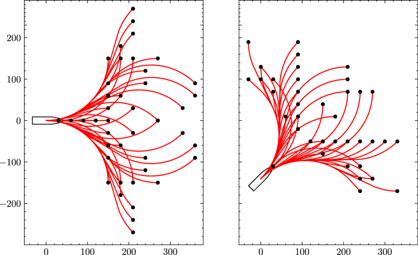
Figure 18: Primitives generated for the full-scale simulation experiments.

To calibrate $\alpha$ in (7), we compared our proposed navigation cost with the actual simulation cost in the Straight trials. Specifically, our goal was to match the ratio of total collision cost $C_{f}$ in (10) to total cost $J$ with the ratio of kinetic energy loss $\Delta K_{\text{ship}}$ to total energy use $E$, meaning

$$\frac{\alpha C_{f}}{L_{f}+\alpha C_{f}}=\frac{\Delta K_{\text{ship}}}{E}.$$ (37)

Solving for $\alpha$ gives us the expression,

$$\alpha=\frac{\Delta K_{\text{ship}}}{E}\frac{L}{C_{f}\left(1-\frac{\Delta K_{\text{ship}}}{E}\right)}.$$ (38)

We used (38) to compute the weights $\{\alpha_{i}\}_{i=1}^{100}$, where each $\alpha_{i}$ corresponded to a sampled Straight trial. We then averaged these weights to obtain $\bar{\alpha}=4.8\times 10^{-7}$, which we used as our calibrated $\alpha$ in the AUTO-IceNav trials.

Regarding the parameters for the ice concentration term in (9), we set $\beta=1$ and used a $51\times 51$ kernel for the image convolution operation. For the optimization stage in Section V, the set $\mathcal{B}_{d}$ consisted of 52 body points equally spaced along 4 rows (similar to Fig. 7 (middle) with $\Delta b=6$ m) where each body point was assigned the default body point weight (26). The weight $\lambda$ for the smoothness term in (V-D) was set to $5\times 10^{4}$ and the lattice planner solution was downsampled to an initial arc length step $\Delta s$ of 4 m.

C-B Physical Experiments

The parameters set in our framework were similar to the values used for the simulation experiments, and were scaled as necessary for the 20 m $\times$ 6 m ice channel. We increased the costmap resolution to 1/16 m $\times$ 1/16 m. At a nominal speed $U_{\text{nom}}$ of 0.2 m/s, we set a corresponding minimum turning radius of $r_{\min}=1.5$ m. To generate the state lattice, we set the discretization for planar position to 0.75 m $\times$ 0.75 m, and we used the same discretization for heading as in the simulation setup. The algorithm from [51] was used here again to generate the motion primitives.

We deviated from the calibration method outlined in Appendix C-A to set the parameter $\alpha$ in (7). Preliminary tests conducted in the OEB indicated that the ice provided limited resistance to ship motion. This meant that in terms of energy use, the optimal path was simply a straight path. As a result, we manually tuned $\alpha$ to apply a higher penalty on the total collision cost $C_{f}$, setting $\alpha=10$. We set the horizon parameter $\Delta h$ to 6 m and the tracking duration parameter $\Delta t$ to 1 s in Algorithm 1.

Appendix D Trial Difficulty Evaluation

A challenge encountered during the physical experiments was ensuring consistency between the three navigation approaches with respect to the initial arrangement of ice floes. Although periodic ‘resets’ of the ice field were performed via manual control of the PSV, the starting ice field configuration remained a source of variation in trial performance. As a result, following the end of running experiments, each of the authors were tasked with assigning a subjective difficulty score for each of the trials. The evaluation process involved examining the first frame captured by the ceiling-mounted camera from a particular trial and responding to the following question:
On a scale from 1 to 5, where 1 is ‘Very Easy’ and 5 is ‘Very Difficult,’ how would you rate the overall difficulty of navigating the ship through the depicted ice field, considering the starting position of the ship and the characteristics of the ice field captured in the provided image?
The evaluations were carried out independently, with the trial sequence randomized, and the navigation information hidden. These scores yielded a mean difficulty for each trial and we binned the scores into three difficulty levels: easy, medium, and hard, with intervals $[1,2.5]$, $(2.5,3.5)$, and $[3.5,5]$, respectively. A summary of the trials per difficulty level is given in Table IV.

	Difficulty level
Method	Easy	Medium	Hard
Straight	8	5	7
Skeleton	3	8	9
AUTO-IceNav	6	7	7

TABLE IV: Number of trials for each method and difficulty level.

References

- [1] A. Chircop, “Sustainable arctic shipping: Are current international rules for polar shipping sufficient?” The Journal of Ocean Technology, vol. 11, no. 3, 2016.
- [2] C. Ø. Hansen, P. Grønsedt, C. L. Graversen, and C. Hendriksen, Arctic shipping: commercial opportunities and challenges. CBS Maritime, 2016.
- [3] Z. Li, J. W. Ringsberg, and F. Rita, “A voyage planning tool for ships sailing between europe and asia via the arctic,” Ships and Offshore Structures, vol. 15, no. sup1, pp. S10–S19, 2020.
- [4] I. Ari, V. Aksakalli, V. Aydogdu, and S. Kum, “Optimal ship navigation with safety distance and realistic turn constraints,” European Journal of Operational Research, vol. 229, no. 3, pp. 707–717, 2013.
- [5] E. Quillérou, M. Jacquot, A. Cudennec, D. Bailly, A. Choquet, and L. Zakrewski, “The arctic: Opportunities, concerns and challenges,” Scientific Fact sheets of the Ocean & Climate Platform, pp. 73–87, 2020.
- [6] C. Ryan, L. Huang, Z. Li, J. W. Ringsberg, and G. Thomas, “An arctic ship performance model for sea routes in ice-infested waters,” Applied Ocean Research, vol. 117, p. 102950, 2021.
- [7] Government of Canada, “Ice navigation in Canadian waters,” May 2019. [Online]. Available: https://www.ccg-gcc.gc.ca/publications/icebreaking-deglacage/ice-navigation-glaces/page05-eng.html
- [8] J.-H. Kim, Y. Kim, H.-S. Kim, and S.-Y. Jeong, “Numerical simulation of ice impacts on ship hulls in broken ice fields,” Ocean Engineering, vol. 182, pp. 211–221, 2019.
- [9] M. Sabolic, “Autonomous and remotely controlled ships and ice navigation,” Master’s thesis, Novia University of Applied Sciences, 2022.
- [10] T. I. Fossen, Handbook of marine craft hydrodynamics and motion control, 2nd ed. John Wiley & Sons, 2021.
- [11] A. Veksler, T. A. Johansen, F. Borrelli, and B. Realfsen, “Dynamic positioning with model predictive control,” IEEE Transactions on Control Systems Technology, vol. 24, no. 4, pp. 1340–1353, 2016.
- [12] K. Murrant, R. Gash, and J. Mills, “Dynamic path following in ice-covered waters with an autonomous surface ship model,” in IEEE OCEANS, San Diego–Porto, 2021, pp. 1–4.
- [13] J. D. Smith, S. Hall, G. Coombs, J. Byrne, M. A. Thorne, J. A. Brearley, D. Long, M. Meredith, and M. Fox, “Autonomous passage planning for a polar vessel,” arXiv preprint arXiv:2209.02389, 2022.
- [14] V. Lehtola, J. Montewka, F. Goerlandt, R. Guinness, and M. Lensu, “Finding safe and efficient shipping routes in ice-covered waters: A framework and a model,” Cold regions science and technology, vol. 165, p. 102795, 2019.
- [15] F. Li and L. Huang, “A review of computational simulation methods for a ship advancing in broken ice,” Journal of Marine Science and Engineering, vol. 10, no. 2, p. 165, 2022.
- [16] J. Thomson, S. Ackley, F. Girard-Ardhuin, F. Ardhuin, A. Babanin, G. Boutin, J. Brozena, S. Cheng, C. Collins, M. Doble et al., “Overview of the arctic sea state and boundary layer physics program,” Journal of Geophysical Research: Oceans, vol. 123, no. 12, pp. 8674–8687, 2018.
- [17] Government of Canada, “Ice glossary,” Nov 2020. [Online]. Available: https://www.canada.ca/en/environment-climate-change/services/ice-forecasts-observations/latest-conditions/glossary.html
- [18] C. Zhang, X. Chen, and S. Ji, “Semantic image segmentation for sea ice parameters recognition using deep convolutional neural networks,” International Journal of Applied Earth Observation and Geoinformation, vol. 112, p. 102885, 2022.
- [19] R. Lubbad, S. Løset, W. Lu, A. Tsarau, and M. van den Berg, “Simulator for arctic marine structures (sams),” in International Conference on Offshore Mechanics and Arctic Engineering, vol. 51296. American Society of Mechanical Engineers, 2018, p. V008T07A020.
- [20] C. Daley, S. Alawneh, D. Peters, and B. Colbourne, “Gpu-event-mechanics evaluation of ice impact load statistics,” in OTC Arctic Technology Conference. OnePetro, 2014.
- [21] R. de Schaetzen, A. Botros, R. Gash, K. Murrant, and S. L. Smith, “Real-time navigation for autonomous surface vehicles in ice-covered waters,” in 2023 IEEE International Conference on Robotics and Automation (ICRA), 2023, pp. 1069–1075.
- [22] M. Stilman and J. Kuffner, “Planning among movable obstacles with artificial constraints,” The International Journal of Robotics Research, vol. 27, no. 11-12, pp. 1295–1307, Nov. 2008.
- [23] T. T. Tran, T. Browne, M. Musharraf, and B. Veitch, “Pathfinding and optimization for vessels in ice: A literature review,” Cold Regions Science and Technology, vol. 211, p. 103876, 2023.
- [24] J.-H. Nam, I. Park, H. J. Lee, M. O. Kwon, K. Choi, and Y.-K. Seo, “Simulation of optimal arctic routes using a numerical sea ice model based on an ice-coupled ocean circulation method,” International Journal of Naval Architecture and Ocean Engineering, vol. 5, no. 2, pp. 210–226, 2013.
- [25] M. Choi, H. Chung, H. Yamaguchi, and K. Nagakawa, “Arctic sea route path planning based on an uncertain ice prediction model,” Cold Regions Science and Technology, vol. 109, pp. 61–69, 2015.
- [26] J. Montewka, F. Goerlandt, M. Lensu, L. Kuuliala, and R. Guinness, “Toward a hybrid model of ship performance in ice suitable for route planning purpose,” Proceedings of the Institution of Mechanical Engineers, Part O: Journal of Risk and Reliability, vol. 233, no. 1, pp. 18–34, 2019.
- [27] C. Zhang, D. Zhang, M. Zhang, and W. Mao, “Data-driven ship energy efficiency analysis and optimization model for route planning in ice-covered arctic waters,” Ocean Engineering, vol. 186, p. 106071, 2019.
- [28] V. Kotovirta, R. Jalonen, L. Axell, K. Riska, and R. Berglund, “A system for route optimization in ice-covered waters,” Cold Regions Science and Technology, vol. 55, no. 1, pp. 52–62, 2009.
- [29] D. Colbourne, “Scaling pack ice and iceberg loads on moored ship shapes,” Oceanic engineering international, vol. 4, no. 1, pp. 39–45, 2000.
- [30] V. Bolbot, A. Sandru, T. Saarniniemi, O. Puolakka, P. Kujala, and O. A. Valdez Banda, “Small unmanned surface vessels—a review and critical analysis of relations to safety and safety assurance of larger autonomous ships,” Journal of Marine Science and Engineering, vol. 11, no. 12, p. 2387, 2023.
- [31] V. Aksakalli, D. Oz, A. F. Alkaya, and V. Aydogdu, “Optimal naval path planning in ice-covered waters,” International Journal of Maritime Engineering, vol. 159, no. A1, 2017.
- [32] T.-H. Hsieh, S. Wang, H. Gong, W. Liu, and N. Xu, “Sea ice warning visualization and path planning for ice navigation based on radar image recognition,” Journal of Marine Science and Technology, vol. 29, no. 3, pp. 280–290, 2021.
- [33] R. M. Gash, K. A. Murrant, J. W. Mills, and D. E. Millan, “Machine vision techniques for situational awareness and path planning in model test basin ice-covered waters,” in Global Oceans 2020: Singapore–US Gulf Coast. IEEE, 2020, pp. 1–8.
- [34] H.-T. L. Chiang and L. Tapia, “Colreg-rrt: An rrt-based colregs-compliant motion planner for surface vehicle navigation,” IEEE Robotics and Automation Letters, vol. 3, no. 3, pp. 2024–2031, 2018.
- [35] J.-y. Zhuang, Y.-m. Su, Y.-l. Liao, and H.-b. Sun, “Motion planning of usv based on marine rules,” Procedia Engineering, vol. 15, pp. 269–276, 2011.
- [36] Y. Kuwata, M. T. Wolf, D. Zarzhitsky, and T. L. Huntsberger, “Safe maritime autonomous navigation with colregs, using velocity obstacles,” IEEE Journal of Oceanic Engineering, vol. 39, no. 1, pp. 110–119, 2013.
- [37] K. Bergman, O. Ljungqvist, T. Glad, and D. Axehill, “An optimization-based receding horizon trajectory planning algorithm,” IFAC-PapersOnLine, vol. 53, no. 2, pp. 15 550–15 557, 2020.
- [38] K. Bergman, O. Ljungqvist, and D. Axehill, “Improved optimization of motion primitives for motion planning in state lattices,” in 2019 IEEE Intelligent Vehicles Symposium (IV). IEEE, 2019, pp. 2307–2314.
- [39] K. Bergman, O. Ljungqvist, J. Linder, and D. Axehill, “An optimization-based motion planner for autonomous maneuvering of marine vessels in complex environments,” in 2020 59th IEEE Conference on Decision and Control (CDC). IEEE, 2020, pp. 5283–5290.
- [40] T. Shan, W. Wang, B. Englot, C. Ratti, and D. Rus, “A receding horizon multi-objective planner for autonomous surface vehicles in urban waterways,” in 2020 59th IEEE Conference on Decision and Control (CDC). IEEE, 2020, pp. 4085–4092.
- [41] G. Bitar, M. Breivik, and A. M. Lekkas, “Energy-optimized path planning for autonomous ferries,” IFAC-PapersOnLine, vol. 51, no. 29, pp. 389–394, 2018.
- [42] E.-L. M. Ruud, M. S. Rundhovde, J. Sandrib, and G. Bitar, “A hybrid-state path planner for asv formations with full-scale experiments,” in 2023 IEEE/RSJ International Conference on Intelligent Robots and Systems (IROS). IEEE, 2023, pp. 4841–4848.
- [43] G. Bitar, A. B. Martinsen, A. M. Lekkas, and M. Breivik, “Two-stage optimized trajectory planning for asvs under polygonal obstacle constraints: Theory and experiments,” IEEE Access, vol. 8, pp. 199 953–199 969, 2020.
- [44] M. Pivtoraiko, R. A. Knepper, and A. Kelly, “Differentially constrained mobile robot motion planning in state lattices,” Journal of Field Robotics, vol. 26, no. 3, pp. 308–333, 2009.
- [45] S. M. LaValle, Planning algorithms. Cambridge university press, 2006.
- [46] T. SNAME, “Nomenclature for treating the motion of a submerged body through a fluid,” The Society of Naval Architects and Marine Engineers, Technical and Research Bulletin, no. 1950, pp. 1–5, 1950.
- [47] H. Kim, D. Kim, J.-U. Shin, H. Kim, and H. Myung, “Angular rate-constrained path planning algorithm for unmanned surface vehicles,” Ocean Engineering, vol. 84, pp. 37–44, 2014.
- [48] J.-B. Caillau, S. Maslovskaya, T. Mensch, T. Moulinier, and J.-B. Pomet, “Zermelo-Markov-Dubins problem and extensions in marine navigation,” in IEEE Conference on Decision and Control, 2019, pp. 517–522.
- [49] X. Liang, P. Jiang, and H. Zhu, “Path planning for unmanned surface vehicle with Dubins curve based on GA,” in IEEE Chinese Automation Congress, 2020, pp. 5149–5154.
- [50] L. E. Dubins, “On curves of minimal length with a constraint on average curvature, and with prescribed initial and terminal positions and tangents,” American Journal of Mathematics, vol. 79, no. 3, pp. 497–516, 1957.
- [51] A. Botros and S. L. Smith, “Multi-start n-dimensional lattice planning with optimal motion primitives,” arXiv preprint arXiv:2107.11467, 2021.
- [52] P. E. Hart, N. J. Nilsson, and B. Raphael, “A formal basis for the heuristic determination of minimum cost paths,” IEEE Transactions on Systems Science and Cybernetics, vol. 4, no. 2, pp. 100–107, 1968.
- [53] S. Alawneh, R. Dragt, D. Peters, C. Daley, and S. Bruneau, “Hyper-real-time ice simulation and modeling using gpgpu,” IEEE Transactions on Computers, vol. 64, no. 12, pp. 3475–3487, 2015.
- [54] H. Kim and C. Daley, “Evaluation of ice loads on offshore structure using gpu-event-mechanics,” in ISOPE International Ocean and Polar Engineering Conference. ISOPE, 2019, pp. ISOPE–I.
- [55] C. Daley, “Energy based ice collision forces,” in Proceedings of the 15th International Conference on Port and Ocean Engineering under Arctic Conditions (POAC), vol. 2, 1999, pp. 674–686.
- [56] D. Dolgov, S. Thrun, M. Montemerlo, and J. Diebel, “Practical search techniques in path planning for autonomous driving,” Ann Arbor, vol. 1001, no. 48105, pp. 18–80, 2008.
- [57] A. Botros and S. L. Smith, “Spatio-temporal lattice planning using optimal motion primitives,” IEEE Transactions on Intelligent Transportation Systems, 2023.
- [58] D. Dolgov, S. Thrun, M. Montemerlo, and J. Diebel, “Path planning for autonomous vehicles in unknown semi-structured environments,” The international journal of robotics research, vol. 29, no. 5, pp. 485–501, 2010.
- [59] M. Zucker, N. Ratliff, A. D. Dragan, M. Pivtoraiko, M. Klingensmith, C. M. Dellin, J. A. Bagnell, and S. S. Srinivasa, “Chomp: Covariant hamiltonian optimization for motion planning,” The International journal of robotics research, vol. 32, no. 9-10, pp. 1164–1193, 2013.
- [60] A. Wächter and L. T. Biegler, “On the implementation of an interior-point filter line-search algorithm for large-scale nonlinear programming,” Mathematical programming, vol. 106, pp. 25–57, 2006.
- [61] J. A. Andersson, J. Gillis, G. Horn, J. B. Rawlings, and M. Diehl, “Casadi: a software framework for nonlinear optimization and optimal control,” Mathematical Programming Computation, vol. 11, pp. 1–36, 2019.
- [62] L. Huang, J. Tuhkuri, B. Igrec, M. Li, D. Stagonas, A. Toffoli, P. Cardiff, and G. Thomas, “Ship resistance when operating in floating ice floes: A combined cfd&dem approach,” Marine Structures, vol. 74, p. 102817, 2020.
- [63] B. Su, K. G. Aarsæther, and D. Kristiansen, “Numerical study of a moored structure in moving broken ice driven by current and wave,” Journal of Offshore Mechanics and Arctic Engineering, vol. 141, no. 3, p. 031501, 2019.
- [64] R. Lubbad, S. Løset, W. Lu, A. Tsarau, and M. van den Berg, “An overview of the oden arctic technology research cruise 2015 (oatrc2015) and numerical simulations performed with sams driven by data collected during the cruise,” Cold Regions Science and Technology, vol. 156, pp. 1–22, 2018.
- [65] V. Blomqvist, “Pymunk: A easy-to-use pythonic rigid body 2d physics library. (version 6.7.0),” 2024. [Online]. Available: https://pymunk.org
- [66] S. Lembcke, “Chipmunk2d: A fast and lightweight 2d game physics library. (version 7.0.2),” 2006. [Online]. Available: https://chipmunk-physics.net/
- [67] R. Yulmetov, R. Lubbad, and S. Løset, “Planar multi-body model of iceberg free drift and towing in broken ice,” Cold Regions Science and Technology, vol. 121, pp. 154–166, 2016.
- [68] A. Steer, A. Worby, and P. Heil, “Observed changes in sea-ice floe size distribution during early summer in the western weddell sea,” Deep Sea Research Part II: Topical Studies in Oceanography, vol. 55, no. 8-9, pp. 933–942, 2008.
- [69] K. Hasegawa, S. Uto, H. Shimoda, D. Wako, and T. Matsuzawa, “Numerical and experimental investigations of managed ice loads acting on fixed conical structure,” in ISOPE International Ocean and Polar Engineering Conference. ISOPE, 2018, pp. ISOPE–I.
- [70] T. Y. Zhang and C. Y. Suen, “A fast parallel algorithm for thinning digital patterns,” Communications of the ACM, vol. 27, no. 3, pp. 236–239, 1984.
- [71] C. Daley, S. Alawneh, D. Peters, B. Quinton, and B. Colbourne, “Gpu modeling of ship operations in pack ice,” in SNAME International Conference and Exhibition on Performance of Ships and Structures in Ice. SNAME, 2012, p. D021S005R001.
- [72] X.-N. Bui, J.-D. Boissonnat, P. Soueres, and J.-P. Laumond, “Shortest path synthesis for Dubins non-holonomic robot,” in IEEE International Conference on Robotics and Automation, 1994, pp. 2–7.
- [73] X. Ma and D. A. Castanon, “Receding horizon planning for Dubins traveling salesman problems,” in IEEE Conference on Decision and Control, 2006, pp. 5453–5458.
- [74] W. Wang, H. Wang, G. Dai, and H. Wang, “Visualization of large hierarchical data by circle packing,” in Proceedings of the SIGCHI conference on Human Factors in computing systems, 2006, pp. 517–520.
- [75] P. Valtr, “Probability that n random points are in convex position,” Discrete & Computational Geometry, vol. 13, no. 3-4, pp. 637–643, 1995.
- [76] T. I. Fossen, S. I. Sagatun, and A. J. Sørensen, “Identification of dynamically positioned ships,” Control Engineering Practice, vol. 4, no. 3, pp. 369–376, 1996.
- [77] T. I. Fossen and T. A. Perez, “Marine systems simulator (mss),” https://github.com/cybergalactic/MSS, 2004.