Continual Evolution in Nonreciprocal Ecological Models
Abstract
Feedbacks between evolution and ecology are ubiquitous, with ecological interactions determining which mutants are successful, and these mutants in turn modifying community structure. We study the evolutionary dynamics of several ecological models with overlapping niches, including consumer resource and Lotka-Volterra models. Evolution is assumed slow, with ecological dynamics producing a stable community (with some strains going permanently extinct) between successive introductions of an invader or mutant. When new strains are slowly added to the community, either from an external pool or by large-effect mutations, the ecosystem converges, after an initial evolutionary transient, to a diverse eco-evolutionary steady state. In this “Red Queen” phase of continual evolution, the biodiversity continues to turn over without the invasion probability of new variants getting any smaller. For resource-mediated interactions, the Red Queen phase obtains for any amount of asymmetry in the interactions between strains, and is robust to “general fitness” differences in the intrinsic growth rates of strains. Via a dynamical mean field theory framework valid for high-dimensional phenotype space, we analytically characterize the Red Queen eco-evolutionary steady state in a particular limit of model parameters. Scaling arguments enable a more general understanding of the steady state and evolutionary transients toward it. This work therefore establishes simple models of continual evolution in an ecological context without host-pathogen arms races, and points to the generality of Red Queen evolution. However, we also find other eco-evolutionary phases in simple models: For generalized Lotka-Volterra models with weakly asymmetric interactions an “oligarch” phase emerges in which the evolutionary dynamics continually slow down and a substantial fraction of the community’s abundance condenses into a handful of slowly turning-over strains.
I Introduction
Ecological and evolutionary processes are inextricably linked. In diverse microbial communities with large population sizes, there is constant interplay between ecological interactions and new genetic variants. Evolution continually creates new variants that interact with the community differently from their parent strains, and these ecological interactions determine the community’s properties and the fate of the new mutants, thereby influencing future evolution. As the increasing body of data from natural microbial communities shows, microbes live in close proximity with one another, with multiple strains and substrains of the same species coexisting in many natural environments Sunagawa et al. [2015], hum [2012], Fierer [2017]. Understanding how ecological interaction webs influence evolution—and vice versa—is crucial for developing a richer picture of microbial evolution in both experimental and natural settings. A major puzzle is the ubiquity of closely related microbial strains coexisting, as evinced by the broad distribution of genomic divergences found within bacterial species apparently occupying the same ecological niche Kashtan et al. [2014], Rosen et al. [2015]. How does such diversity evolve and persist without clear ecological differences stabilizing the coexistence of strains? Theory is needed to develop distinguishable scenarios for the evolution and maintenance of fine-scale biodiversity in large microbial populations.
Even in controlled laboratory experiments with initially-clonal microbial populations, the development of ecology is inevitable. Although apparent selection pressures in the laboratory can be held constant, evolution in “simple” environments still generically results in the diversification and coexistence of different strains Rosenzweig et al. [1994], Friesen et al. [2004], Maharjan et al. [2006]. Long after increases in fitness (as measured by competition with the ancestor) have slowed and populations seem to be well adapted to laboratory conditions, it has been observed, e.g. in the E. coli experiments of Richard Lenski, that evolution continues without further decrease in the rate of successful mutations Good et al. [2017]. Furthermore, diversification and coexistence of lineages is observed even in such experiments designed to be simple enough to eliminate ecological effects Lenski [2017], Good et al. [2017]. Remarkably, even in laboratory experiments on bacterial populations without an external nutrient supply—which might be expected to exhibit severe resource limitation and diversity collapse—diversification and phenotypic turnover is found to continue over a timescale of years Finkel and Kolter [1999].
With interacting bacteria and phage populations, there is clear evidence—both experimental and observational—for the continual turnover and diversification of microbial lineages Ignacio-Espinoza et al. [2020], Marston et al. [2012], Buckling and Rainey [2002]. The “Red Queen hypothesis” Van Valen [1973] is often invoked to describe such arms-race evolutionary dynamics of hosts and pathogens. In the current work we use “Red Queen dynamics” more generally to describe continual turnover of biodiversity in a community without successful invasions of new mutants becoming rarer, and we look for such dynamics in other ecological contexts.
Inspired by observations of microbial populations, we aim to understand what generic scenarios can emerge in the long term dynamics of evolution of ecological communities. We are particularly interested in robust behaviors that obtain across a range of parameters and models—such “phases” of eco-evolutionary dynamics present a set of qualitative possibilities that one can hope to compare with experiment or observation. The phases that we study emerge in the limit of large biological complexity: high-dimensional phenotype and interaction spaces upon which evolutionary and ecological processes play out. Looking for phases that are robust in the limit of high phenotypic dimensionality —roughly the number of phenotypic properties of organisms that affect the ecological dynamics—increases the likelihood that the conclusions we draw are somewhat universal and relevant to natural systems, which are more complex—in multiple ways—than the simple models we study.
In order to understand what long term behaviors emerge in high-dimensional eco-evolutionary models, it is useful to first think separately about the dynamics of evolution and ecology, initially in a well-mixed population with no spatial structure. A further simplification is natural for large microbial populations: that the dynamics are essentially deterministic, with demographic fluctuations negligible except close to extinctions.
Evolution without ecology: In a static environment without ecology, gradual evolution of a large almost-clonal population can be caricatured as gradient ascent on a complex fitness landscape. The fitness landscape is a map from some high-dimensional organismal phenotype to the “fitness”: a misleading but canonical term for a measure of reproductive success that is surely not a single quantity except in the simplest non-ecological contexts. The emergence and fixation of beneficial mutations drives the population to high-fitness regions of phenotype space and evolution slows down as the population approaches one of the (typically) many local maxima of the fitness landscape De Visser and Krug [2014]. However in high dimensions, this simple intuition is only part of the story: the phenotype will generally spend a long time wandering around saddles before “committing” to a particular maximum, which is likely to be only marginally stable Fisher [2021].
In large populations with an abundant supply of mutations, the evolutionary dynamics of the population of genotypes is complex, with simultaneous exploration of multiple phenotypic directions: this regime has not been much studied theoretically. However if there is no ecology except resource limitation capping the total population size, eventually the supply of beneficial mutations will become so limited that the population will again become almost clonal. By contrast, in an extrinsically changing environment, the fitness landscape depends on time, and is better caricatured as a “seascape.” Not surprisingly, a continually changing environment can lead to evolutionary dynamics which proceed indefinitely without slowing down Agarwala and Fisher [2019] and produce continually turning-over diversity: again, such phenomena have not been much studied for large populations in high phenotypic dimension.
Ecology without evolution: Just as evolutionary dynamics of large populations can display rich behavior even without ecology, ecological dynamics with no evolution can exhibit various behaviors, with globally stable, multistable, and chaotic states all possible in simple models Bunin [2017], Opper and Diederich [1992], Blumenthal et al. [2024]. The most-studied contexts are ecological dynamics of top-down assembled communities, which consist of a large number of species brought together with their abundances obeying some prescribed ecological dynamics. The simplest ecological phase that obtains at long times is a state in which species abundances reach a globally attracting stable fixed point with some number of species (the stable community) having nonzero abundance and the rest going extinct, unable to reinvade even if reintroduced. As the diversity of this assembled community increases, the stable phase can yield to a more complicated behavior exhibiting multiple attractors and transient chaos, which remains only partially understood Bunin [2017], Blumenthal et al. [2024], Ros et al. [2023]. Chaotic fluctuations in the high-diversity unstable regime lead to many extinctions and the system settles down to one of many possible stable communities or limit cycles, but these fixed points are generically unstable to invasion by some of the extinct strains. A population of dormant spores that germinate and resuscitate extinct populations can sustain the chaos for times exponentially long in the lifetimes of the spores, but as a matter of principle such dynamics do not constitute a true ecological phase Pearce et al. [2020].
Interplay of ecology and evolution: To bring evolution and ecology together, we focus here on the slowly evolving limit in which the ecological dynamics are much faster than the evolutionary dynamics and spatial mixing is fast enough to be ignored. Motivated especially by the puzzle of fine-scale diversity, we are primarily interested in multiple strains of a single species with overlapping niches. This regime is the hardest in which to find sustained diversity and continual evolution because it does not allow short-term transient coexistence driven by continual invasions of new mutants, which was studied in refs. Xue and Goldenfeld [2017], Huisman et al. [2001], Yan et al. [2019].
We study models in which the ecological dynamics are simplest, converging to a (usually) globally attracting fixed point with some strains permanently extinct. Under slow evolution, do the resulting eco-evolutionary dynamics remain diverse and continually turn over in a “Red Queen” steady state, or does evolution get progressively slower and slower? Do generalist mutants take over and cause the diversity to crash? Are there multiple different phases of eco-evolutionary dynamics for different parameter regimes?
It has been shown that Red Queen dynamics emerge generically in models of an almost-clonal population evolving in a high-dimensional fitness landscape with a small amount of environmental feedback Fisher [2021]. In these models, the fitness landscape—now better caricatured as a “snowscape”—changes as the evolving population affects its environment. For even a small amount of such feedback, the population wanders through phenotype space without settling down to a stable fixed point, due to selective forces that arise from the gradient of its continually-modified fitness landscape. Universality emerges in these models in the limit of large phenotype dimension, with different microscopic models displaying similar phase diagrams, including a phase of sustained evolutionary chaos Fisher [2021].
In the eco-evolutionary models we study here, ecology acts loosely as a manifestation of feedback between organism and environment, with the “environment” of any particular strain set by its interactions with the rest of the community, and thus subject to change every time a new mutant arises in the community. Can natural models of this process result in a Red Queen phase of evolution? If so, what sets the diversity of the community in this phase?
Some previous work has found that ecological communities, although capable of sustaining extensive diversity through standard mechanisms of resource competition Armstrong and McGehee [1980] lose much of their diversity when they start to gradually evolve either by small mutations or by the introduction of independent species Shoresh et al. [2008], Schippers et al. [2001]. These results were argued to deepen the puzzle of the extensive diversity observed in nature. However, the models in which such results have been reported are complicated enough that analytical understanding is difficult, and generality of the claims is not clear—indeed other work has suggested that phenotypic complexity allows the gradual evolution of high diversity Doebeli and Ispolatov [2010].
Evolutionary dynamics: The evolutionary process we study involves adding strains one by one to an ecological community, with extinctions permanent when they occur. Once extinct, a strain will never be able to re-emerge, even if conditions become favorable for its growth. Therefore the order in which strains are introduced influences the fate of the community. However, the statistical properties of the evolving community for large phenotypic dimension depend only on the pool from which invaders are drawn, rather than on the specific properties of the invaders.
Previous work has studied the process of adding strains into ecological models without permanent extinctions Tikhonov and Monasson [2018], Serván and Allesina [2021], Capitán et al. [2009], where re-invasion of previously-extinct strains is possible if conditions later become favorable for them. This process eliminates the important difference between communities assembled all at once (top-down) and gradually (bottom-up): the latter is our focus.
A large amount of work by theoretical ecologists and statistical physicists has focused on ecological models that are nongeneric because they admit a Lyapunov function which is always increasing under the eco-evolutionary dynamics Altieri et al. [2021], Tikhonov and Monasson [2017], Cui et al. [2020], Biroli et al. [2018]. The existence of such a Lyapunov function depends on the symmetry of ecological interactions Marsland III et al. [2020], e.g. through perfect efficiency in the conversion of nutrients to biomass, which does not hold in biological systems. Therefore the generality of conclusions drawn from such models is unclear. In the current work we focus on generic behavior, drawing conclusions away from the special slice of parameter space with a Lyapunov function. Indeed we will show that, under evolution, the behavior of models with a Lyapunov function is qualitatively different from the general case. Several other studies Bonachela et al. [2017], Law et al. [1997], Nordbotten and Stenseth [2016] have noted the importance of nonreciprocal or asymmetric ecological interactions for reaching a state of continual evolution—we will provide further evidence for this conclusion in the high-diversity limit, which complements the more often-studied low-diversity case Bonachela et al. [2017], Law et al. [1997]
Models: We are interested in dynamics of closely related strains, where differences between strain interactions with one another are sums of many positive and negative effects. To caricature this biological complexity, we parameterize the strain-to-strain differences in phenotypic properties as random variables drawn from some distribution. This approximation of unknown complexity by randomness is a useful way to get a sense of general patterns of behavior that might apply across a range of ecological-evolutionary situations May [1972].
In the simplest models, strains interact with one another directly, with all pairwise interactions chosen from some specified ensemble. These models, which include generalized Lotka-Volterra interactions Bunin [2017], suffer from a lack of strain phenotypes which, when present, dictate how each strain interacts with any other prospective strain. As a result, the effective phenotypic dimensionality in Lotka-Volterra models is infinite. Problematically, such models do not generally admit a straightforward way of drawing random mutants correlated with a parent strain in the community Mahadevan et al. [2023]. Nonetheless we will study the Lotka-Volterra eco-evolutionary dynamics in the case of independent invaders added to the community. This simple limit is instructive for understanding evolution driven by mutant strains correlated with their parents.
To explicitly study the effects of parent-mutant correlations we introduce structure into the ecological interactions, considering the case where they are mediated by a collection of chemicals (or resources) in the environment. Each strain has a phenotype which describes its effect on the resources and the resources’ effect on its growth rate—these phenotypes consequently determine the inter-strain interactions. Small mutations correspond to having highly correlated parent and mutant phenotypes, with the amount of similarity between mutant and parent playing an important role.
The phenotype of each strain in such consumer resource models is given by its growth and consumption rates for each of the resources. The number of resources—or more generally, interaction-mediating chemicals—is the key quantity . This number sets the dimensionality of the environment and of the interactions between consumers. It also sets a natural scale for the number of strains that can coexist: in the models we study here, the diversity is bounded above by , and “high-diversity” means that the number of coexisting strains is . The limit of large —surely biologically relevant Doebeli and Ispolatov [2010]—will allow us to analyze statistical (hopefully universal) properties of the resulting eco-evolutionary dynamics.
When mutational effects are sufficiently large, we find that key aspects of the evolutionary dynamics are captured by the dynamics of bottom-up assembly (with extinctions), wherein phenotypically independent invaders enter the community serially. The understanding from this simplified regime gives us qualitative insight into differences between a top-down-assembled and an evolved community, along with a framework for understanding the Red Queen phase that occurs for correlated mutants.
In order for the Red Queen phase to be robust, it must be stable to the presence of “general fitness” mutations which increase the growth rate of a strain regardless of the composition of the community. These general fitnesses appear naturally in models of resource competition, where they correspond to the growth rates of strains in isolation. Metabolic tradeoffs, which constrain the width of the general fitness distribution, are sometimes invoked to sustain high levels of diversity in ecological settings. These tradeoffs can be strict Posfai et al. [2017], Caetano et al. [2021] or—more realistically—allow some variation in the total metabolic budget Cui et al. [2020]. Without strict tradeoffs, can consumer resource and Lotka-Volterra models evolve towards a diverse state in which the distribution of extant general fitnesses is narrow? Or does evolution constantly push into the tail of the general fitness distribution and fail to reach a steady state? Do generalist species emerge and reduce diversity by outcompeting other strains?
Our main result is that there exists a robust high-diversity Red Queen phase of eco-evolutionary dynamics characterized by continual evolution and turnover of biodiversity, and that this phase occurs across a range of parameters and models. Importantly, the Red Queen phase persists in the presence of general fitness differences, as long as their distribution decays fast enough. The tail of the general fitness distribution controls the probability of successful invasion and therefore the rate of turnover in the steady state, but otherwise does not limit the diversity.
II Consumer resource model
II.1 Ecological dynamics and stable communities
We first study a standard model of resource competition with externally-supplied resources (or more generally, interaction-mediating chemicals), and an assembled population of different strains that consume these resources (see refs. Cui et al. [2020], Marsland III et al. [2020], Tikhonov and Monasson [2017], Posfai et al. [2017]). The ecological dynamics of this consumer resource (CR) model are
| (1a) | ||||
| (1b) | ||||
where the are the populations of strains, labeled by Roman indices and the are resource abundances labeled by Greek indices . The resource supply vector has components , and and are respectively the death rate of the consumers and the decay (or dilution) rate of the resources. Without substantial loss of generality, we take all the to be equal and given by a constant , and we set to reduce the number of parameters without changing the qualitative behavior. The matrices and respectively parameterize the growth and feeding rates of each consumer on each resource: the phenotype of strain is the corresponding row of and taken together, so that the dimensionality of phenotype space is . The elements of and consist of some positive mean—an average growth or feeding rate—in addition to a heterogeneous part that varies between strains and resources. Ref. Cui et al. [2020] studied the ecological dynamics of a symmetric version of this model with . Although we expect and to be positively correlated, some amount of asymmetry—arising from, e.g., varying efficiencies in utilization of resources—is generic, and we will show that this asymmetry is important for the dynamics of interest to us.
For closely related strains, the differences between interactions will be sums of positive and negative effects: thus we treat and as random variables drawn from some distribution. With the interpretation of consumption and growth, one expects the elements of and to be positive, though a small fraction being negative (corresponding loosely to crossfeeding or inhibitory effects) does not change the behavior. For simplicity we draw the elements from gaussian distributions with means , and variances , respectively. The choice of a gaussian distribution is convenient as we will later take advantage of this structure to evolve strains by drawing from the ensemble of interactions conditional on inequality constraints. However, as we show in Section IV.5, the upper tails of the distributions of the elements of and play an important role in the evolution.
We parameterize elementwise correlations between the gaussian entries of and by , where is the Pearson correlation coefficient between and , and the symmetry parameter parameterizes the similarity between growth and consumption rates. The ratios and determine what fraction of the entries of and are positive; we consider and so that most entries are positive. With the choice of there are only three important parameters other than and : , and , with setting a scale for the consumer abundances (Appendix A). Without loss of generality we will set , and .
The degree of correlation, , between the feeding and growth rates plays an important role: presumes identical efficiencies of conversion between resources and biomass between strains Cui et al. [2020]. This symmetry guarantees the existence of a Lyapunov function (see Appendix A) that is always increasing along the ecological (and later evolutionary) dynamics of the CR model Marsland III et al. [2020]. However for generic the dynamics do not have a Lyapunov function, which makes a big difference for the evolutionary behavior as we will see shortly.
One must supplement the deterministic dynamics of Equation 1 with a small abundance threshold below which strains go extinct: their abundances are then set to zero and cannot recover. In large populations the dynamics and extinctions are driven deterministically by growth rate differences, so we neglect demographic noise. Starting from positive initial conditions, the strain abundances in the CR model generally reach a fixed point with some fraction of strains going extinct and others persisting at nonzero abundance. We denote by the community of extant strains: those with positive fixed point abundances. For small enough —less than some multiple of —the fixed point is generally stable and cannot be invaded by any of the extinct strains. For large , in the parameter ranges of interest, the stable uninvadable community is highly likely to be unique Marsland III et al. [2020]. The breakdown of this uniqueness above a critical value of (discussed for a related model in ref. Blumenthal et al. [2024]), will not play a role in the evolving communities of interest here.
At the ecological fixed point of the CR dynamics, the abundances of the extant strains and the resources are determined (with ) by
| (2a) | ||||
| (2b) | ||||
| (2c) | ||||
with the strains extinct and unable to reinvade. Whether a strain can invade from low abundance is determined by the sign of its invasion fitness
| (3) |
If is negative, strain cannot invade.
The total population size, , is of order , which is roughly for our choice of parameters. (We have kept the dependence on explicit because it carries a physical meaning and characterizes the environment. In our simulations all of its components are : the effects of changing are discussed briefly in Section V.)
We define the extant strain diversity, , as the number of strains left in the community at the ecologically stable fixed point. In accordance with the competitive exclusion principle Armstrong and McGehee [1980], the maximum that can stably coexist at a fixed point is , as seen from the insufficiency of the fixed point conditions otherwise. For natural choices—including ours—of the ensemble of interactions, the typical number of strains that can stably coexist at a fixed point scales linearly with with a coefficient less than . This linear relationship between the diversity of the community and the number of resource-mediating chemicals is expected to be generic across a range of consumer resource models with heterogeneous interactions, with the statistics of the interactions affecting the prefactor in the scaling Cui et al. [2020]. In ecological language, the number of potential niches is but not all of these can be filled.
Measures of diversity: In the ecological literature many different measures of diversity of communities have been introduced Daly et al. [2018]. We will use , the total number of species in the community, which is sometimes called the richness. Other popular measures are the Shannon diversity: the weighted average of , and the inverse Simpson index (inverse participation ratio in physics terminology), given by . If there is a broad distribution of abundances in a community, these measures can be quite different. However in our models, as we shall see, the distribution of abundances is not very broad so which measure we use does not affect our conclusions. For simplicity we refer to as the “diversity.”
II.2 Evolutionary processes
Evolution by independent invaders: We now focus on slow evolution of stable communities in the CR model, assuming a clean separation of timescales between evolution and ecology. If the resource dynamics are fast enough, they can be integrated out to yield equations for the strain dynamics which reach the same fixed point irrespective of the resource timescale—we can therefore assume fast resource dynamics to simplify our dynamical equations without affecting the evolutionary behavior. The ecological dynamics of the community run until a fixed point is reached. Then a single new strain is introduced, and the ecological dynamics again run until a fixed point is reached. The ecological time scale thus does not affect the evolutionary dynamics of primary interest.
We first study the case of independent invaders into the community. Although this process is sometimes referred to as “bottom-up assembly,” it will give us insight into evolutionary dynamics with large-effect mutations. We start with a single strain of consumer and a collection of resources, and repeatedly add an unrelated consumer strain drawn from the gaussian phenotype ensemble. We define an epoch as the unit of time corresponding to a successful invasion followed by the relaxation of the ecological dynamics to a fixed point. Although the length of an epoch in ecological time varies between epochs, in our case of slow evolution the ecological timescale is not important.
With each new strain added, we find a stable uninvadable ecological fixed point of the community either by integrating the dynamical equations with a small extinction threshold, or by the more efficient iterative algorithm described in Appendix D. Once is sufficiently large, we expect that, with high probability, this fixed point is the unique stable uninvadable fixed point for the collection of extant strains in each epoch—this intuition is based on analogy with the assembled community in which the uninvadable fixed point is unique as long and are of similar size Bunin [2017], as is the case in our evolving system where the size of the extant community plus the new invader is analogous to .
Invaders: In order for a new strain, labelled , to be able to invade, it must have positive invasion fitness . Furthermore, if it successfully invades, its fixed point abundance will be approximately proportional to , with the constant of proportionality determined by the properties of the community into which invades, as can be seen by a perturbative analysis for large . The dot product between the growth vector (the th row of ) and the resource vector of the community determines the invasion fitness of strain . Therefore when we draw the phenotype of —consisting of -dimensional vectors and —from their gaussian ensemble, we condition on , which drastically speeds up numerics when the evolution pushes the extant distribution of interactions to have large mean, making invaders with very rare Vrins [2018].
The resource availability vector can be thought of as a modified version of the supply vector , where the availability of resource is reduced from by a factor of . Therefore alignment between and results in a contribution to the invasion fitness of strain that is independent of the other strains in the community—this contribution to the invasion fitness is a form of general fitness, here defined as , which captures the average performance of strain against all of the resources at the rate that they are supplied by the environment, and thus scales with the magnitude of the resource supply vector. Therefore for an invader has a community-independent contribution proportional to the general fitness as well as a community-dependent contribution from the ecological interactions. We refer to the community-dependent part of the invasion fitness as the drive, which will be defined more precisely for the models we introduce in Section III.
It is useful for analysis to extend the definition of the invasion fitness to strains already in the community: for we define as the growth rate strain would have if it were removed from the community and then reintroduced at low abundance. This quantity arises naturally in the mean field description of ecological models (Section IV and Appendix F) and we will sometimes refer to it as the bias, consistent with previous work Pearce et al. [2020]. The bias is therefore an invasion fitness appropriately defined for strains both inside and outside the community. Differences between biases of different strains come from both the general fitnesses and the drives, and such differences are responsible for the differential growth and extinction of strains.
As we show in Appendix C, in a randomly assembled community the selective differences—related to differences between general fitness terms —are first order in the phenotypic differences, proportional to , while the variations in the drives are second order, proportional to both and , where we have defined , and weighted averages and similarly for . Therefore the selective differences comprise the dominant contribution to the width of the bias distribution, larger by a factor of than the contribution from the drives. For large the selective differences determine both the ecological and early-stage evolutionary dynamics and can, at least initially, strongly limit the diversity. Previous work Cui et al. [2020] has forced the contributions to be comparable by scaling the mean and variance of and as , while in fact it is their mean and standard deviation that should be the same order in a biologically-motivated model. We will later show that in a long-evolved community, the variations in the general fitnesses become much smaller, indeed comparable to the variations in the drives. However—importantly—this feature must be shown to emerge rather than assumed.
II.3 Eco-evolutionary dynamics
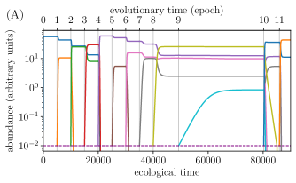
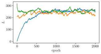
To explore the eco-evolutionary dynamics, we choose resources with well away from the special value for which there is a Lyapunov function: we investigate that special case later. Starting from a single strain (), Figure 1A shows the ecological dynamics of the strain abundances in Equation 1 (with resources integrated out), punctuated by well-spaced evolutionary events when an invader comes in at the start of each new epoch. When the system has reached an ecological fixed point, a new strain is introduced, drawn randomly from the ensemble of independent strains conditioned on being able to invade (the conditioning speeds up numerics, since new strains which cannot invade will not affect the community). The new strain joins the community and the ecological dynamics find a new stable fixed point at which the abundances of the other strains are perturbed, with some strains possibly going extinct. Thereafter another strain is introduced.
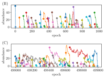
From now on, we focus on the evolutionary dynamics and ignore the ecological transients at the beginning of each epoch that drive some strains extinct and others to nonzero abundances. The changes caused by invading strains can be visualized over longer times by coarse-graining the time resolution from ecological to evolutionary epochs and tracking the fixed point abundances of strains (calculated with the algorithm of Appendix D). Such strain abundance trajectories are shown near the beginning of the evolution in Figure 1B and, after much evolution, in Figure 1C. We show only a few of the strains for ease of visualization.
Primary quantities of interest are the extant strain diversity , the population mean general fitness (with angular brackets denoting weighted averages over the community), and the probability that a randomly chosen strain can invade, denoted . In addition to the community level properties, we are interested in the statistical properties of strains including the distributions and temporal correlations of their abundances , their general fitnesses and their evolutionary lifetimes which we call (see Section IV.3 for more details).
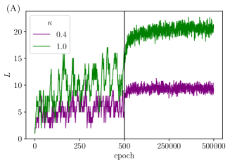
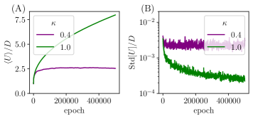
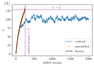
The evolution of the diversity for is shown in purple in Figure 2A. Starting from a single strain, initially grows fast and then slows down, appearing to saturate at at long times, for which we plot a moving average. As shown in Appendix I for a related model that we will introduce shortly, the fluctuations in are resulting from rough independence of strains along with robustness of the community to perturbations (Section IV.2). For , it thus appears that the evolution converges to a Red Queen steady state. Note that although for these parameters remains rather small, we later show that it is expected to be of order , here only , in the large limit of primary interest. The modest used here was needed for convergence to steady state in reasonable time.
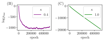
Further evidence for the Red Queen state for is shown in Figures 2B, where the invasion probability of a new strain, , after initially decreasing rapidly, saturates at long times (albeit to an extremely small value). This behavior can be understood through the general fitnesses. Figures 3A and B show in purple the mean and width, respectively, of the extant , distribution. Initially the mean increases, but then saturates at a value of order with the strains all having similar . The evolution therefore pushes far out into the tail of the general fitness distribution, making it very hard for other strains to invade. We shall show in Section IV.5 that the width of the distribution of extant general fitnesses, scaled by the mean consumption rate of the resources—which is what enters in the growth rate of the strains (Appendix C)—shrinks during evolution until it is similar to the width of the drive distribution. At this point the intrinsic (general fitness) and community-derived (drive) parts of the bias contribute similarly to bias differences between strains. Once this occurs, the distribution of extant stops pushing higher and we reach a Red Queen evolutionary steady state with a roughly steady rate of turnover.
In an evolutionary steady state (when it occurs) we denote averages over time by overbars. Because of the turnover of strains, in steady state temporal averages should be equal to averages over the ensemble of strains.
Turnover of strains: In steady state, one new strain invades in each epoch and on average, one extant strain goes extinct. This means that a strain remains in the community for an average of epochs and the rate of turnover of strains is per epoch. This is seen in Figure 1 where at early times when is small, strains do not survive long, while in the long-time steady state with larger they survive longer on average even though there are still strains that go quickly extinct, as we discuss in Section IV.3.
The continual turnover of strains together with the plateauing of mean that in the Red Queen phase, strains that successfully invade and later go extinct will have a substantial chance of being able to reinvade once the community has sufficiently turned over and lost memory of its state at the extinction time of the strain. Each strain keeps “memory” of its general fitness which, because it was able to invade earlier, must be similar to that of the other strains in the steady state.
While these simulations provide strong evidence for a Red Queen steady state for , quantitatively they are problematic. It is apparent from Figure 2B that for the ensemble of strains we have used, the invasion probability of a new invader is unrealistically small in the steady state (). In Section III.1 we will introduce a family of models in which at steady state can be much larger, and in Section IV.5 we analyze how the choice of the and ensembles affects the invasion probability in steady state, and show that the very small observed above is an artifact of the gaussian phenotype ensemble we have used for numerical convenience.
Totally symmetric ensemble: We now show that the perfectly-symmetric case, , which possesses a Lyapunov function (see Appendix A), behaves very differently from the ensemble for which there is no Lyapunov function. From the green trajectory of the diversity in Figure 2A, it is difficult, based only on the dynamics of , to know whether a steady state obtains by the end of the simulation. Invading strains must increase and there is no absolute upper bound of in the ensemble of all possible invaders. Therefore even if saturates, there cannot be a steady state. The larger gets, the more unlikely that adding new strains can increase it further—thus the probability of invasion, must steadily decrease, as indeed seen in Figure 2C. Concomitantly, the mean general fitness pushes further and further into the tail of its distribution as shown by the green trajectory in Figure 3A, while the standard deviation of the decreases (green curve Figure 3B) due to the steepening of the distribution around (see Section IV.5).
Because of the Lyapunov function, we conclude that there is no Red Queen steady state for . It is interesting to note that, in spite of the gradual increase of , stays far away from its upper bound of . Indeed, stays below its maximum value of for a randomly assembled community with Cui et al. [2020]. However it is not clear whether under evolution might eventually reach or exceed this bound.
Evolution via mutations: So far we have considered independent invaders in the CR model. In Appendix B we study the evolutionary dynamics when invaders are correlated with a parent strain chosen with probability proportional to its abundance in the community. Indexing the parent by and the mutant by , we introduce a parameter : the elementwise Pearson correlation coefficient between and and between and . Given a parent, we draw mutants from this ensemble (while also preserving correlation between and ): therefore the correlation between and is also . Our main finding is that for sufficiently far from —i.e. mutations of substantial effect—the eco-evolutionary phenomenology is similar to the independent invader limit .This finding allows us to base qualitative conclusions for true evolution on results from independent invaders.
| CR | Consumer resource model (Equation 1) |
|---|---|
| LV | Lotka-Volterra (Equation 5) |
| number of strains in initial pool | |
| phenotypic dimension; number of resources | |
| number of extant strains at fixed point | |
| abundance of strain | |
| general fitness in CR model; | |
| invasion fitness = bias | |
| fractional abundance of strain ; | |
| drive = community-dependent component of bias | |
| width of drive distribution | |
| general fitness; intrinsic component of bias | |
| distribution from which are drawn | |
| scale of distribution | |
| community average of (unless otherwise stated) | |
| value of in the saturated assembled community | |
| vector of resource supply rates | |
| growth rate matrix | |
| feeding rate matrix | |
| matrix of growth rate differences; mean | |
| matrix of feeding rate differences; mean | |
| community mean “fitness”; | |
| pairwise strain interaction matrix | |
| correlation between growth and feeding; | |
| symmetry parameter for LV model; | |
| niche parameter of LV model; | |
| probability of a new variant successfully invading | |
| correlation between parent and mutant | |
| evolutionary time average of | |
| scale of distribution around (Equation 21) |
III Simplified models
The saturation of the community-mean general fitness in the Red Queen eco-evolutionary steady state for is a manifestation of continual evolution in an ecological system. We seek simpler—but still robust—models that display such a Red Queen steady state, but which allow us to separate out and independently tune the importance of ecological interactions and general fitnesses. The two related models that we shall study both have a generalized Lotka-Volterra form, but with different ensembles for the interaction matrix between strains. The first model is a linearized version of the CR model with the resource dynamics integrated out, yielding a maximum rank for the strain interaction matrix. The second model is of a more standard Lotka-Volterra type, with direct interactions drawn from some ensemble and diagonal “niche” interactions enabling substantial diversity to coexist. For some ranges of parameters, both of these models exhibit a Red Queen phase characterized by constant turnover of biodiversity. In addition they allow us to isolate the effects of the general fitnesses on the eco-evolutionary dynamics.
III.1 Linearized resource model
In the Red Queen steady state of the CR model, the mean of , the total consumption rate of resource , is large compared to its variations (Figure 14A), suggesting an expansion in these variations. In addition, the total population of the ecosystem is roughly constant on evolutionary timescales (Figure 14B), due to the large mean of and relative to their variations—this motivates us to separate out the mean part of these matrices from their variations, and introduce zero-mean residual interaction matrices and . We work in terms of fractional abundances rather than absolute abundances, and integrate out the resource dynamics since these do not affect the fixed point.
Expanding in the differences between resources and between strains yields general fitnesses at first order and interactions at second order (Appendix C). The simplified model that we introduce, and refer to hereafter as the linearized resource model, or simply the linearized model, is
| (4a) | ||||
| (4b) | ||||
The term is a Lagrange multiplier, equal to , which incorporates the average effects of growth, death, and resource depletion, and keeps the population constant with . Here, the per capita growth rate of each strain is a linear function of the abundances of all the other strains, with a quadratic part from that is the same across all the strains and includes the average general fitness. Differences in general fitness are parametrized by , the selective differences between strains, which play the role of the in the CR model. As the means have been subtracted off, the residual part of the resource vector can have components which are negative. then measures deviations of resource availability away from some positive baseline.
The structure of Equation 4 is that of a generalized Lotka-Volterra model or system of replicator equations (discussed further in Section III.2), where the interaction matrix between strains, denoted by , has a structure inherited from the and matrices via , where and are matrices. We take each element of and to be gaussian distributed with mean zero and unit variance, with no correlations within or . Elementwise correlations between and are again parameterized by via .
The off-diagonal entries of have mean zero and standard deviation while the diagonal entries have mean and standard deviation . The parametrically-larger (for large ) diagonal entries thus endow the interactions with sufficient niche structure to stabilize the dynamics. (Note that would result in unstable behavior with the diagonal entries of having positive mean.) As in the CR model, the number of resources sets the dimensionality of phenotype space, with the phenotype of strain comprised of along with the th rows of and . The maximum number of coexisting strains at a stable fixed point of the linearized model is equal to and will generally be proportional to with a prefactor less than .
When , is a convex Lyapunov function for Equation 4. If additionally , we have which is nonpositive. For nonzero , the Lyapunov function gets an extra piece and can be of either sign, though it remains a convex function of the .
We will take the general fitnesses to be drawn from a distribution , which for most of this paper is gaussian with mean and variance . In Section IV.5 we show that the value of determines the early evolutionary behavior and the value of at steady state, with the shape of the large- tail of playing a controlling role. As the community evolves and the distribution of extant pushes into the tail of , the effective —the variance of the extant —decreases. Therefore tuning to be small a priori mimics the effects of prior evolution and allows us to study communities that have been evolving for a long time, without the long initial evolutionary transient.
As discussed previously in Section II.2, for the CR model in Equation 1, the width of the distribution is a factor of larger than the width of the drive distribution. In the linearized model, this corresponds to , since the distribution of the drives in a diverse community has width. However, in the Red Queen steady state, as we shall see, the first and second order—in —components of the growth rate of each strain become comparable to one another. Thus we mostly consider , and sometimes set , which shortens the transient period of evolution before the steady state is reached—and enables analysis—but does not change our conclusions. In Section IV.5 we also discuss non-gaussian distributions of the , which affect quantitative properties but not the basic phenomenology.
III.2 Lotka-Volterra model
In addition to the linearized model of Equation 4, we have studied the generalized Lotka-Volterra (LV) model (or replicator equations) Diederich and Opper [1989] which take the form
| (5) |
with . The LV model has similar structure to the linearized model of Section III.1; the difference lies in the statistics and parameterization of the interaction matrix . Instead of the with random and of the linearized resource model, in this LV model the are themselves gaussian random variables with , , and for , with other covariances zero. Here is the symmetry parameter tuning between predator-prey-like interactions for and competitive interactions for : a rough correspondence with the linearized model for positive is . The negative diagonal term is a “niche” parameter that measures the strength of self-interaction relative to inter-strain interaction, playing a similar role to in the linearized model. Our parameterization of the LV equations differs from a common parameterization in which interactions have nonzero mean Bunin [2017]: here the matrix captures variations in interaction magnitudes, with taking the role of the mean interaction strength Pearce et al. [2020]. As in the linearized model, when the interactions are symmetric (), is a Lyapunov function of the dynamics, though in contrast to the linearized model Tikhonov and Monasson [2017], it can become a nonconvex function of the for large enough Biroli et al. [2018].
The LV model has a similar ecological phase diagram to the CR model and linearized models, with a globally attracting fixed point of the dynamics when is sufficiently small. The maximum at a stable uninvadable fixed point scales as with a -dependent coefficient Opper and Diederich [1992]. Note that the scale of the drive distribution is in the LV model, as opposed to in the linearized model, since the overall scale of the entries in the LV model is smaller by a factor of than in the linearized model.
In the LV model, unlike in the linearized and CR models, strains cannot be characterized by finite-dimensional phenotypes. Although one can attempt to define a phenotype of strain by along with its corresponding row and column of , this phenotype depends on the rest of the community and thus changes—or grows in dimension—as the community turns over.
III.3 Properties of invaders
Having defined the simplified ecological models of interest, we will now specify the process by which they evolve. We first discuss general facts about invaders introduced into the community, and then define the specific parameterization of invaders that we have used for simulations.
As in the CR model, whether a new strain successfully invades the extant community or not is determined by its invasion fitness or bias, now written as with in the LV model and in the linearized model. Splitting the bias up into the general fitness piece , the Lagrange multiplier and the drive is useful since it separates the intrinsic and extrinsic contributions to the bias. Strains with positive bias can invade the community and reach abundance proportional to their bias, whereas strains with negative bias go extinct. As in the CR model, we sample properties of the invader conditional upon Vrins [2018]. A strain’s extinction occurs when its abundance goes to in the ecological dynamics or, equivalently, when its bias goes negative.
In the LV model, the lack of phenotypes makes attempts to parameterize correlations between parent and mutants ad hoc for general Mahadevan et al. [2023], so we confine our study to the case of independent invaders. An invader strain is generated by drawing a new row and column of from the original gaussian ensemble with , and by drawing general fitness from a gaussian distribution with mean and variance . Therefore the invasion probability of an independent invader is where is the standard normal CDF.
In models with phenotypes, such as the CR or linearized model, there is a natural way to generate mutants through small changes to the phenotype of an extant parent strain. This procedure creates a mutant whose interactions with all other strains are similar to those of its parent. In our gaussian ensemble, the probability of any parent generating a mutant that can invade is the same—therefore we can, in an unbiased way, simply select a parent with probability proportional to its abundance.
The parameter describes the correlation between parent and mutant . The mutant phenotype is drawn from an ensemble that preserves , , and . We fix the desired correlations by drawing the phenotype of as
| (6a) | ||||
| (6b) | ||||
| (6c) | ||||
where the , and are uncorrelated standard normal random variables. This choice ensures that the elements of the interaction matrix have correlations for . The invasion probability of a mutant drawn from this ensemble is given by
| (7) |
where is the standard normal CDF. In this paper we restrict study to large effect mutations, with . The behavior as , corresponding to small effect mutations, is both interesting and biologically relevant: we will discuss it in depth in future work.
III.4 Evolution in the linearized resource model
The motivation for introducing the linearized model is to capture the phenomenology of the CR model—a Red Queen state with continual turnover but roughly-constant mean general fitness and —in a simple setting where the effects of the general fitnesses can be separated out from the interactions, and with a shorter transient period before the steady state is reached. We begin by describing the basic phenomenology of evolution in the linearized model of Equation 4, with the evolutionary dynamics of Equation 6. In general, the evolutionary dynamics are parameterized by , , , and , the size of the initial pool of strains. However only plays a role in the transient behavior: the evolution converges to the same state independent of the initial diversity as illustrated in Section III.5 for the LV model.
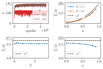
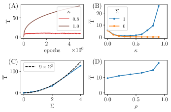
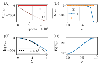
In Figure 4A we plot the dependence of on evolutionary time for two values of : and . (We have here chosen to yield higher diversity than the used for the CR model.) Starting from a single strain, there is a transient during which the diversity builds up, after which both trajectories flatten out. Figure 5A shows the trajectories of the Lagrange multiplier, —analogous to the mean general fitness in the CR model, which clearly showed the difference between the behavior with and without a Lyapunov function. For , saturation of indicates a Red Queen steady state and results in saturation of . By contrast, for , continues to increase and concomitantly decreases: there is no Red Queen phase.
To investigate the Red Queen phase in the absence of a Lyapunov function, we study the long-time averages , and for ranges of the parameters , , and mutant-parent correlation . (Note that the typical of interest is better characterized by than as can fluctuate by large amounts especially when is large as discussed in Section IV.5.) Figures 4, 5 and 6 display these quantities across a range of , , and . The important conclusion from these simulations is that the Red Queen phase obtains across a range of parameters for , and that parameter choices, though affecting the length of the pre-steady state transient and the qualitative properties of the steady state, do not eliminate the Red Queen phase. Therefore the Red Queen state can be qualitatively understood by studying just a few values of the relevant parameters. The value of sets the overall scale of but, as long as it is large, does not matter much—we therefore choose a large and for our simulations. This choice yields a large number (roughly ) strains surviving in the Red Queen phase yet keeps away from the non-generic behavior.
In Figure 4A, the observed is compared with the curve which is the maximum in a top-down assembled community with and drawn from the gaussian ensemble for the linearized model (see Section IV.1). We see that from simulations is less than this naive upper bound, as will be discussed in Section IV.2. In Section IV.5 we will give scaling arguments for how and at steady state depend on and : some of these scalings are compared with simulations in Figures 5 and 6.
III.5 Evolution in the LV model
Given the apparent similarities between the CR and linearized models, it is natural to ask how the eco-evolutionary phenomenology in the random Lotka-Volterra model resembles or differs from these: in particular whether the difference in the ensemble of the interaction matrix between the LV and linearized models matters. In Appendix E we investigate evolution—by independent invaders—in the LV model across a range of and , the symmetry and niche parameters defined in Section III.2. For a range of we find a Red Queen phase analogous to those of the CR and linearized model, with the product of and a function of determining the number of strains in the steady state; we have also checked that a Red Queen phase obtains for nonzero . Similarly to in the linearized model, in the Red Queen phase fluctuates around a mean value that is less than the maximum from a top-down assembled community. The gap between the realized and the assembled upper bound as a function of is shown in Figure 15A. This gap diverges as , meaning that in this regime, the Red Queen steady state is much less diverse than the largest possible community assembled top-down. In contrast, in the linearized model, the gap is bounded over the whole range of . The distinction is not surprising: there is no regime of the linearized model that corresponds to the negative cross-diagonal correlations in that characterize the LV model with negative .
The fact that a top-down assembled community can be substantially larger than the evolved community in the LV model allows us to check that the Red Queen phase obtains across a range of initial number of strains, . In particular, since the top-down assembled community can have , there are situations in which there is a naturally-findable stable ecological community that is unstable to evolution, with decreasing as the evolving community converges to the Red Queen phase. Figure 7 shows this behavior in the LV model for and , with approaching from both above or below, depending on the of the initial community. Therefore, even in simple models, the question of whether evolution increases or decreases diversity from a top-down assembled initial condition has no general answer Shoresh et al. [2008], Doebeli and Ispolatov [2010].
Breakdown of Red Queen phase: Although we find a robust Red Queen phase for a range of and in the LV model, closer investigation of the effect of reveals an interesting feature. The evolutionary dynamics in the LV model change sharply with , appearing to exhibit a discontinuous transition around for . For a Red Queen phase obtains, while for we find a phase in which the rate of successful invasion is ever-slowing and a few strains rise to high abundance. We therefore name this phase the “oligarch” phase of eco-evolutionary dynamics—a counterpart to the Red Queen’s monarchy. The oligarch phase is discussed further in Section V, and we leave its fuller analysis for future work. For now, we note that there does not appear to be an oligarch phase in the linearized or CR models: the Red Queen steady state obtains for all , albeit with and respectively diverging as approaches and evolutionary transients correspondingly lengthening.
IV Analysis
In order to understand the phenomenology of the Red Queen phase described above, it is useful to first discuss the top-down assembled community of the linearized model in which all strains are brought together at once with dynamics determined by their ecological interactions. An understanding of the ecological phase diagram in this setting is informative for analyzing the Red Queen phase, and gives us an idea of how and scale with various parameters in the Red Queen phase.
To analyze the eco-evolutionary dynamics, we will introduce a particular limit of the linearized model which reduces to the LV model with . With the further simplifications of independent invaders and —yielding the simplest ensemble of the LV model—we can exactly solve for the steady state of the evolutionary dynamics in the limit of large diversity. Key quantities are the distribution of strain abundances in an evolved community—strikingly different than a top-down assembled community—and temporal correlation functions of strain abundances in evolutionary time.
We then add in selective differences, presenting general scaling arguments for the dependence of , and on , which build on the intuition gleaned from the assembled communities. We discuss subtleties associated with long-lived strains with anomalously large , generalize to different distributions, , and show how the primary pathologies of the gaussian distribution can be alleviated.
IV.1 Assembled communities
In a top-down assembled community of the linearized model, all the strains are initialized at positive abundance, and are governed by the deterministic dynamics of Equation 4 without a sharp extinction cutoff. The cavity method Roy et al. [2019] can be used to analyze both the statics and dynamics of the assembled community with initial strains and resources, in the limit of large and with the ratio constant. The spirit of the cavity method—in the static case—is to consider a large community to which one adds, separately, one new strain and one new resource: these each act as small perturbations to the fixed point of the community. The abundance of the new strain is determined by its invasion fitness, modified by the community-wide response to its introduction, and the new resource is treated similarly. One then enforces self-consistency conditions that the statistics of the strains and resources in the community are the same as the statistics of the newly added strain and resource. These conditions rely on the community being assembled with independent interactions, since then the independently-drawn invading strain and resource are from the same ensemble as the rest of the community. By solving the self-consistency equations one can extract abundance distributions of and , and solve for and as a function of , and . Similar results can be obtained for the CR model Cui et al. [2020] and—more simply—for the LV model Opper and Diederich [1992].
The cavity method also allows one to derive self consistent equations for the ecological dynamics Roy et al. [2019], in addition to their fixed point—we use a variant of this method to understand the evolutionary dynamics in Section IV.3.
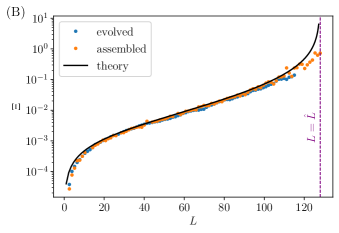
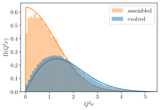
Details of the static cavity analysis for top-down assembled communities with gaussian are in Appendix F, for both the linearized and LV models. We find that generically the linearized model exhibits two phases as a function of the ratio . For , when is small enough, there is a unique stable globally attracting fixed point, uninvadable by the strains that are going extinct: this fixed point is described by the cavity solution and the community diversity is . The abundances of the strains in the stable community are distributed as a truncated gaussian so that there is a constant density of abundances near zero. (Figure 9 shows this feature—and its agreement with the result of the cavity calculation—for the LV model which is similar to the linearized model in this respect.) The strains destined for extinction have negative invasion fitnesses with a distribution that also has a constant density near zero. Thus the assembled community has many close-to-marginal strains.
When the number of the strains assembled, , becomes larger than a (-dependent) critical value , at which , the cavity solution becomes unstable and chaotic dynamics or multi-stability ensues Blumenthal et al. [2024]. We use a hat to denote the values of quantities at this phase transition, and refer to the community at this transition as saturated. The number of initial strains needed to achieve this saturated state, , diverges as as long as . Therefore for and the cavity solution is always stable. When the picture for remains the same, while at there is a transition (for ) to a nongeneric “shielded” phase Tikhonov and Monasson [2017] in which —the maximum allowed by competitive exclusion—and this state is highly marginal.
With an extinction threshold, even for the ecological dynamics will generally reach a stable fixed point with . However the resulting community will generally be unstable to re-invasion by some of the strains that had gone extinct. Furthermore, in this super-saturated regime there are multiple possible stable communities, almost all of them invadable by some of the extinct strains. Which community occurs will thus depend on the initial conditions. The question of whether or not stable uninvadable communities are likely to exist for large is unresolved except for the special case where there is an absolute maximum of the convex Lyapunov function. However it is believed that even if such fully-stable fixed points exist for , they may attract only an exponentially small fraction of initial conditions Cugliandolo et al. [1997], Fisher [2021].
We can glean insights about the properties of an evolved community with from an analysis of the near-saturated assembled community, since after long period of evolution, a large number of strains—many more than —will have had a chance to invade the evolved community. Naively, one might think that the end result will be similar to assembling the whole community at once. However as we shall see, the evolved community never becomes saturated in the way that an assembled community can be.
We would like to understand the behavior for which is what occurs “naturally” (e.g. from the CR model): we thus focus for now on this limit. In the linearized model the saturated assembled community has for all and, for ,
| (8a) | ||||
| (8b) | ||||
The reciprocal of scales with the fraction of surviving strains, and therefore the invasion probability of a single independent invader is of order .
We conjecture that the forms of the scalings of and with in the assembled community also describe the time-averaged quantities in the Red Queen steady state, i.e. that and , albeit with unknown coefficients. The scalings in Equation 8, along with the guess that , motivate the approximate theory curves in Figures 4, 5 and 6: these are consistent with numerical data from the Red Queen phase. In Section IV.5 we give an argument that the conjectured scalings of and with should indeed be expected on evolutionary grounds.
IV.2 Fragility of assembled and evolved communities
In the eco-evolutionary Red Queen phase, ecological communities remain stable, but are different from top-down assembled communities since their interaction statistics are conditioned on evolution and, crucially, they would be unstable to invasion by some fraction of previously extant strains that have gone extinct. An indication of this distinction, shown in Figures 4 and 8A, is the diversity of the Red Queen phase: is smaller than in saturated assembled communities, , across the range of . When a community is assembled one strain at a time with permanent extinctions, it is not possible to reach as high diversity as reached by top-down assembly. What is responsible for this gap between in the Red Queen phase and from the saturated assembled community? The answer is associated with the relative fragility of the two states.
The transition between phases in the assembled community is marked by the onset of an instability in the cavity solution. This instability entails the divergence of a community-level property that we call the fragility and denote by . The fragility quantifies the variance of the changes in strain abundances in response to a random perturbation to the growth rates of all the strains. Concretely, if for each strain we add a small independently random term to its growth rate, with and variance (loosely like applying random fields in magnetic systems), the fragility is defined by . The fragility can also be written as where the are elements of the susceptibility matrix of the community. Deep in the stable phase the fragility is small, as small perturbations to strains’ growth rates do not cause abundances to reshuffle by much. However as the transition is approached and nears , the fragility diverges, indicating a breakdown in the stability of the cavity solution. In Figure 8B we plot the fragility, computed directly from the interaction matrix, for both an evolving and top-down assembled community across a range of . In both cases, increases with , and in the evolving community it plays an important role in the Red Queen phase, as we now discuss.
Each new invader adds a small random part to the biases of the other strains. Invader , which reaches a stable abundance , contributes to the bias of each strain . The variance of this random perturbation is for the linearized model. This is multiplied by a factor of to yield of order and therefore . For a typical strain with , this perturbation will be small. However in a top-down assembled community, the lowest abundance strains will have smaller than typical by a factor of , and of these will have abundance less than the magnitude of the perturbation. This implies that the invasion will drive the bias of of the lowest abundance strains negative, causing their extinction. Concomitantly, if we do not enforce permanent extinctions, the perturbation will increase the bias of a similar number of barely-extinct strains and these will enter the community. As long as is not large, this number of extinctions and invasions will be small. As , diverges and the assembled community will be shaken a lot by a single additional strain.
The behavior of an evolved community—with permanent extinctions—in response to a small random perturbation is quite different. When the community has just been assembled, if it is close to saturated, a single invader will drive a fraction of the strains with extinct. As this is strains, will initially decrease (Figure 7). Under the perturbations from further invasions, the density of low abundance strains will be hollowed out by this process which is like diffusion with an absorbing boundary condition at zero: This results in a density of abundances that goes linearly to zero as (see Figure 9). The diffusion coefficient of the abundances in evolutionary time is proportional to the fragility of the community, so if is large, then the perturbations are amplified and more extinctions result, on average, from each successful invader. As the diversity grows, we expect that (as in the top-down assembled communities), the fragility also grows. When it is large enough that on average one extinction is driven by each invasion, the diversity stabilizes. This must thus occur while the fragility is not too large suggesting—although not implying because of the complexities on conditioning on the evolutionary history—that the Red Queen state will be less diverse than the maximal assembled diversity, , as observed in Figure 8A. Note that the ratio depends on the value of (Figure 4B); this is presumably due to the dependence of on .
In the special case of perfect symmetry ( for the linearized model and for the LV model), approaches at long times despite the lack of a Red Queen steady state. We do not have an explanation for this apparent saturation of the diversity through gradual assembly.
In recent work, de Pirey and Bunin Arnoulx de Pirey and Bunin [2024] have observed and studied a similar phenomenon of depletion of low-abundance strains due to continual perturbations to the community from invading strains. These authors looked at a purely ecological model but with small migration from a mainland that prevents total extinction of any strain. Species rising up from the brink of extinction play the role of invaders in our evolutionary model. The similarities between this ecological model and our work are discussed in Appendix L. A primary difference is due to the migration-induced boundary condition: As there is a flux of strains both in and out, the steady state distribution of does not vanish as and the boundary condition must be determined self-consistently from the ecological dynamics. In the evolutionary problem we study, more analytical progress is possible due to the simplicity of the extinction boundary condition in contrast to that which arises from migration.
IV.3 Exact solution in simplest case
Having understood some features of the eco-evolutionary phenomenology by comparison with the saturated assembled community, we now proceed to directly analyze the evolutionary dynamics for a particularly simple choice of parameters.
With , there are correlations between the cross-diagonal elements of the interaction matrix , as in the case of the LV model. These correlations induce complex memory into the evolutionary dynamics since the effect of an invader on a strain in the community via feeds back via onto . This feedback on is coherent across the extant strains with magnitude proportional to (or ). Thus the properties of a strain in the community depend on its effects on the other strains over all the epochs since its invasion. This fact makes the evolutionary dynamics difficult to analyze (like the ecological dynamics in ref. Pearce et al. [2020]), as the form of this memory kernel needs to be self-consistently determined along with the dynamics of the strains abundances in evolutionary time. We set this analysis up in Section IV.4 but do not carry it through.
However, there is a limit of the linearized model that is simple: if we take and while keeping the product finite, we can rescale the interaction matrix by a factor of to obtain the LV model with and , implying in the Red Queen phase. (Note that in this limit, the elements of become gaussian and the off-diagonal elements are .) The fact that for the interaction matrix has no correlations across the diagonal makes the feedback effects smaller by a factor of (and of random sign) and hence negligible—therefore the analysis that we undertake becomes tractable. We first treat the case of , , and then set up the general structure of the cavity calculation for nonzero and , before heuristically analyzing the effects of .
Our analysis of the Red Queen phase proceeds by means of a dynamical cavity method, which is one way of carrying out dynamical mean-field theory (DMFT) as used in systems with quenched randomness Roy et al. [2019]. The idea is to consider the evolutionary-time dynamics of a focal “cavity strain” labelled , that could potentially enter the community, persist for some number of epochs, and later go extinct. For , the abundance of the cavity strain while it is in the community is determined by its bias, if positive. In this simple case the strain’s feedback on itself averages to zero so that in the limit of large (Appendix F). However the bias, , changes in evolutionary time . If the strain attempts to invade at epoch , then its abundance in the community at all later times is
| (9) |
where is the indicator function which is unity when its argument is true and zero otherwise. The cavity strain’s abundance is only nonzero as long as its bias remains positive—and it goes irrevocably extinct once its bias goes negative. Therefore the statistics of the cavity strain abundance are determined by the statistics of its bias together with the permanent extinction condition.
To carry out the analysis, one needs to make an Ansatz for the statistics of the cavity bias, and then calculate the statistics of the cavity abundance as filtered through the extinction condition. One then enforces self consistency, which relates the dynamics of strain abundances in the community to the original statistics of the cavity bias. This is possible since the cavity drive is simply , which has gaussian correlations for large . Since the are independent and not conditioned on properties of the community, we have, for the LV model with the being ,
| (10) |
where the sum is over all strains that have invaded before time —most of which will be extinct at or and therefore not contribute to the correlation function. For large , the average over , denoted by the overbar, is not needed: we expect to be “self-averaging” and depend only on the time-difference (up to subdominant corrections). A particular role is played by the equal-time correlations: , with the last equality for the LV model where . (In the linearized model carries an additional factor of .)
The self-consistency condition at the heart of the cavity method is that the autocorrelation of the cavity strain, averaged over trajectories and invasion time , is the same as the autocorrelation function of strains in the community conditioned on having the same general fitness . The correlation functions of strains in the community, weighted-averaged over the distribution, determine via Equation 10. The Lagrange multiplier has to be adjusted to fix (just as is determined for the static ecological cavity analysis of Appendix F).
We now specialize to the simplest case where all are zero. Simulations of the , Lotka-Volterra model (Figure 15B) suggest that in this case and we make the Ansatz that this is exact. Hoping for some luck, we then make the simplest possible Ansatz for the statistics of : namely that it has an exponentially decaying correlation function . This Ansatz for the correlation function can be translated into a stochastic process that determines :
| (11) |
with the time measured in epochs and white noise satisfying (angular brackets here denote averages over the stochasticity caused by invaders). The white noise represents the changes in the community from adding independent invaders which cause the diffusive changes in abundances discussed in Section IV.2. The deterministic term is, roughly, regression to the mean of zero, which can be seen to arise from the correlation between and due to the same elements of appearing in both quantities Mahadevan et al. [2023]. The quantities and are (for now) phenomenological parameters that must be fixed later by self-consistency. The advantage of having a Markovian stochastic differential equation for , along with , is that the method of images can be used to find the statistics of with an absorbing boundary condition at zero, conditioned on its invasion at time .
In order to calculate the right hand side of the self-consistency condition Equation 10, we need to calculate the two-time correlation function of . Since (with all ) the strains are statistically equivalent, we can calculate for the cavity strain entering the community with the initial condition of ), averaged over the stochasticity in Equation 11. We then average this correlation function over and . We know that is determined by Equation 9 with since .
From our Ansatz, the initial is distributed as a gaussian random variable with standard deviation , conditioned to be positive (as epochs are measured per successful invasion). In order to calculate from the strains in the community, we integrate over all initial times —equivalent to fixing and integrating over all —and over all starting abundances weighted by the thalf-gaussian measure. We work with all times in evolutionary epochs, so that the integral of the distribution of for is the rate of successful invasions per unit time, which is in these units.
A self-consistent solution is possible if the result of this calculation gives an exponentially decaying correlation function that can be equated with the correlation function of the cavity drive . Fortunately, this turns out to be the case. An additional self-consistency condition fixes . Put together, these conditions allow us to solve for and . We then compute the diversity . These calculations are carried out in Appendix H. The key results are the self-consistent exponential solution for the correlation function
| (12) |
and the steady state diversity given by
| (13) |
The timescale of the decay of the correlation function is , consistent with the community turning over every successful invasions. We additionally find that and .
Figure 10 compares the analytical results to numerics on the , LV model. As increases in Figure 10A, the numerics get closer to the large- regime in which the theory holds, and in steady state approaches from above. Figure 10B shows the scaled correlation function versus scaled time , which agrees well with Equation 12.
From the self consistent solution we can also calculate the distribution of strain lifetimes, where the lifetime of a strain , denoted , is the number of evolutionary epochs for which it has nonzero abundance. In Appendix H we find a distribution
| (14) |
Figure 10C shows good agreement between this analytical result and the numerics: decays exponentially at large as expected, and has an integrable divergence as , due to the distribution of invaders having a constant density at low abundance. These invaders go extinct very quickly as discussed in Section IV.2. Note that, as successful invaders must balance extinctions, : the mean diversity is equal to the average strain lifetime in epochs.
The dynamic cavity method also enables us to determine the distribution of strain abundances in steady state, as the solution to a Fokker Planck equation with appropriate boundary conditions and with a source term for the invading strains (Equation 72). This solution is plotted in Figure 9, in reasonable agreement with the numerical result for the distribution of abundances in the Red Queen phase. As anticipated in Section IV.2, there is a marked difference between the abundance distribution in the eco-evolutionary steady state and the saturated assembled community abundance distribution with . In the assembled community the abundance distribution is a truncated gaussian—a half-gaussian at saturation. By contrast, in the Red Queen steady state, the density of strains vanishes at low abundance due to the constant jostling of the community by invaders which knock low-abundance strains extinct: the effective diffusion coefficient capturing this process is proportional to the fragility.
For the LV model with , the fragility can be calculated directly due to the simple relationship between and . For each strain with positive bias, so the susceptibility to a change in growth rate is (Appendix F). However the change in each causes a small random change of the biases of all the other strains, which increases the effective variance of the random field, and so on. Summing up these effects Mahadevan et al. [2023] yields a total effect of random ’s given by with the fragility . This result does not depend on how the community is formed, or on the selective differences if they are present. It shows right away the maximum size of a stable community is , which is saturated for an assembled community. For the evolved community, cannot be large—otherwise multiple strains would be driven extinct by each invader. Thus , as we find in numerics.
IV.4 General cavity formulation
We now generalize the cavity analysis away from , . For in the LV model the analysis is particularly complicated. (For in the linearized model it is even more so as both resources and strain dynamics have to be analyzed as in the ecological cavity calculation of Appendix F.) The bias and abundance of a focal strain are no longer simply related as in the case: due to the feedback of the strain on itself via its influence on the other strains, will depend both on its bias and an additive term arising from the feedback integrated over all times since its invasion. Therefore the analog of Equation 9 for is
| (15) |
where
| (16) |
with a memory kernel that must be determined self-consistently. It will include an instantaneous—on evolutionary time scales—part from the invader’s ecological feedback on its own abundance, in addition to a slow memory part that extends over many epochs Fisher [2021]. Both the memory effects and the part of mean that the cavity strain will not go extinct when goes through zero, but instead at some other time when first goes negative.
The statistics of the drives are determined by the extant community, but is no longer a simple exponential. Nevertheless, one can write an effective stochastic equation for :
| (17) |
with another memory kernel and still white noise which represents the diffusion-like effects of an invader on the other strains discussed in Section IV.2. The Fourier transform of is related, via a Weiner-Hopf factorization, to the Fourier transform of : denoting the transforms by tildes, we have
| (18) |
with analytic in the upper half of the complex plane.
In principle, to proceed one assumes a —or equivalently a and —as well as (and if , also . Then one computes conditioned on invading at time . By averaging over , and , one can enforce the self-consistency of using Equation 10, as for the case. Then is self-consisted from calculating the response of to a change in its bias, and is self-consisted to ensure . In the linearized model with resources, the resources have to be handled by a cavity method as well but their effects can be integrated out to give a more complicated relation between strain abundances and , with replaced by and replaced by (Appendix F).
Unfortunately, even numerical analysis of the self-consistency conditions to determine the memory functions and is likely challenging Roy et al. [2019]. However the above structure allows us to glean some insights.
In the absence of selective differences, all strains are statistically similar and the systematic decrease in should make the strain lifetime distribution decay exponentially at long times. This suggests that both the memory kernels and will decay exponentially at long times, as will the correlation function of the drives, . To explore the effects of feedback, we carried out simulations of the LV model for , , and , and plotted in Figure 19B. We see that indeed decays exponentially at long times for all these , with some deviations at shorter times in opposite directions for positive and negative . Concomitantly, as increases, the timescale over which decays, scaled by the overall turnover time of epochs, grows.
There is no sign of marginality in the exact solution for , —therefore the Red Queen phase should be robust to small perturbations, as evinced by these simulations for . The heuristic arguments below suggest that the robustness extends as well to arbitrarily large , and numerical results suggest that it extends up to modest—although not all—: see Section V for more discussion of this point. In contrast to the LV model, simulations of the linearized resource model suggest that the Red Queen phase obtains for all .
IV.5 Effects of selective differences
The Red Queen phase that obtains for in both the linearized and LV models has many properties in common with the case we have analyzed. Here we discuss more systematically the effects of a distribution of general fitnesses, focusing first on the distribution of strain lifetimes, , and then on the correlation function , whose decay at large is dominated by strains with large . We then consider large and give scaling arguments for how the community evolves into the tail of the distribution, which allows us to find the dependence of and on . When the distribution of extant pushes into the tail of the distribution, all of the steady-state properties are determined by the form of —thus we consider non-gaussian of the form . We will also comment on with bounded support.
Correlation function and lifetime distribution: From the general structure of the cavity analysis, we can attempt to understand the behavior of a strain with anomalously-large (we suppress the strain index for notational convenience). The behavior is simplest in the LV model with , for which the only memory is in which still has mean zero and determines the abundance of the cavity strain when in the community (Equation 9). Extinction occurs when , i.e. which is unlikely for large since will fluctuate around , staying far from zero for a long time. The rare event for to decrease to has, quite generally for well-behaved stationary gaussian processes, probability of order for sufficiently large , where the extinction is most likely to occur once the correlation has decayed significantly from . However, we need to examine if the cavity Ansatz of a well-behaved gaussian process is consistent when large can occur.
The effects of large are most clearly understood by their effects on the average strain lifetime , which is equal to in steady state. The naively-predicted behavior is that the average lifetime of strains with large is at least as long as the inverse of their estimated asymptotic extinction rate. Thus, conditioned on , the mean is . The unconditional expected lifetime is then
| (19) |
with the invasion probability of a strain with general fitness , which for large will be close to unity. The effects of large on the correlation function are related to their effects on the lifetime distribution, since long-lived strains have abundance for most of their lifetime (with coefficient for the LV model). Thus is dominated at long by the fraction of strains whose lifetime is at least . We thus expect that for large ,
| (20) |
with the factor likely yielding factors. If falls off sufficiently rapidly, the integral in Equation 19 that determines is convergent, and the correlation function concomitantly decays to zero. For , one finds with decaying similarly so that . The gaussian case, , is marginal with the integrals over convergent only for small enough where the critical value is determined by . For and , decays as a -dependent power of .
When in the gaussian case, as well as for any , the integrals over that determine both and the correlation function appear to diverge. Thus this naive analysis, which relied on the gaussian rarity of large fluctuations, must break down—or the Red Queen steady state must cease to exist. In order to better understand what happens for , we turn to numerics.
In Appendix K we explore numerically the effects of for the LV model with gaussian across a range of . In spite of the naive expectation from the above analysis of a loss of steady state for large enough , the numerics show a steady state even for . The distributions of appear to have a finite first moment and still appears to decay to zero (Figure 21). What are possible resolutions of this apparent discrepancy between the cavity analysis and the observed behavior?
Since our simulations are for only modestly-large up to , finite- corrections to the cavity analysis could be substantial for the range of parameters we investigated here: maybe such corrections enhance the robustness of the steady state to large . It is also possible that fluctuations in , which are expected in any case to increase as increases (Appendix K), become much larger than the expected in the regimes where the naive cavity analysis breaks down. Large positive fluctuations in will eventually drive extinctions of strains that had anomalously large when they invaded, although it is unclear how such large fluctuations could leave the predicted average properties unchanged.
Another possibility is that the gaussian Ansatz for the statistics of breaks down in the tail even for large —with some non-trivial scaling with and —invalidating the rare event analysis for large . This could make the rate of “barrier” crossing of much larger than the naive gaussian estimate, perhaps associated with anomalously long-lived fluctuations in that themselves arise from the persistence of large- strains.
We discuss further in Appendix K some of these issues but for now must leave the subtle effects of longish tails of unresolved. For the present purposes, we note that empirically, even for quite large , the primary conclusions of the cavity analysis, here and below, are at least semi-quantitatively good.
The above discussion has focused on the simplest case of the LV model. For , or in the linearized model with independent of , there are additional complications that could arise for when the correlation function develops a long tail, which will induce long tails to both the memory kernels. It is unclear whether or not the persistent memory in and (Equations 16 and 17), will change the behavior qualitatively and make the simple analysis break down even when it is still valid for . However the numerics show that the naive analyses are roughly correct for average properties of the evolved communities.
Evolutionary transients and steady state for : We now analyze the evolutionary dynamics in the limit of large assuming that either decays sufficiently rapidly for the problems with rare events not to matter, or that the analysis ignoring them is correct for averaged properties. In what follows we mainly discuss the linearized model in which the distribution of biases has width—this can be translated to the LV model by recalling that there the width of the bias distribution is with scaling similarly.
For , there is a long evolutionary transient during which the distribution of extant creeps into the tail of . The tail of therefore determines the long term evolutionary dynamics, including—when it occurs—the properties of the Red Queen phase. As the population-mean (and therefore ) increases, the extant ’s will be near to with the scale of their variation set by the shape of near . The width of the extant distribution will be of order
| (21) |
which decreases with increasing for decaying faster than exponentially and increases with for decaying slower than exponentially. At any point in the evolution, once , the distribution of extant is concentrated around and the system behaves as if there were an exponential distribution of the with scale .
Given this exponential approximation to the general fitness distribution, it is helpful to understand the behavior of an assembled community with an exponential when the extant are large enough that the lower bound of does not matter—this will determine a key relationship between and . If we assemble a large number of strains with an exponential distribution of general fitnesses , for sufficiently large the ecological cavity analysis (Appendix G) yields an assembled community with in the linearized model (and in the LV model). We therefore expect that during the transient evolution, the community will reach a slowly-changing quasi steady-state with diversity given, at any point in time, by .
We have shown above that the behavior of determines the behavior of . How does depend on during the evolutionary transient and into the Red Queen steady state? The increase of is tied to the increasing mean , denoted , so we are led to analyze how changes in evolutionary time. Each successful invader must have . The probability density of conditioned on invasion is (see Appendix of ref. Mahadevan et al. [2023])
| (22) |
where and is the CDF of the standard normal distribution. It follows that
| (23) |
As a result, when , there is a steady state and is roughly constant in evolutionary time, with its value depending on the form of the function . During the transient and in steady state, which saturates at . (Note that for constant—as in the case of a pure exponential —there is no special for which vanishes, so there is no natural scale for .)
We can now proceed to analyze the behavior with , for which . For stretched exponential decay of , corresponding to , is an increasing function—therefore will run away to positive values with concomitantly decreasing. The diversity thereby crashes and eventually the community will reduce to a single strain that goes extinct when a fitter strain invades. Even if is small and seemingly unimportant, eventually a rare large will emerge, leading to large enough that , and therefore to diversity crashing.
For (including the gaussian case ), initially is of order . From the above analysis, we expect diversity .
With large, invasions will tend to increase , thereby decreasing and increasing . Eventually will decrease to , independent of , so that the widths of the extant and distributions are comparable. Concomitantly, will saturate at , and will saturate at , with .
We are now in a position to analyze the transient evolutionary dynamics that occur when and . For large , as it will be initially, the change in due to a successful invasion by strain is roughly , coming from the fitness increment multiplied by the typical abundance . Since the fitness increment is and , the change in per invasion is . On average is positive until the contribution of becomes comparable to , at which point and .
The transient behavior is found by integrating up the typical change per invasion: roughly until is close to . Thus during the transient
| (24) | ||||
| (25) |
for a duration
| (26) |
after which the steady state ensues.
An important observation is that some aspects of the Red Queen steady state for large are independent of details of the distribution and of : in particular, for large , is independent of , as seen in Figure 4 for gaussian , since becomes large enough that the distribution of the extant has width, irrespective of .
To compare with our numerics for gaussian , we specialize to in which case . Here we have and . This scaling is similar to the saturated assembled community (Section IV.1), in which was conjectured to scale with . During the long initial transient, and with the transient lasting for a number of epochs , consistent with the rapid growth of transient length with in Figures 4, 5 and 6. In Appendix J, we check that this predicted transient behavior of agrees with numerics. Perhaps surprisingly, given the potential problems caused by large ’s and discussed earlier in this section, the predicted transients and steady state behavior seem to persist for gaussian even when .
Invasion probabilities: Because of large -dependent coefficients, even moderate values of can make unrealistically small at steady state. For , and , the invasion probability at steady state is less than (Figure 5D) which suggests that , which determines via , has a value for , substantially smaller than the value for the top-down assembled community, (Equation 8a).
In the CR model, invasion probabilities are even smaller: as discussed earlier, the width of the general fitness terms dominates over that of the interactions by a factor of , corresponding to in the linearized model. Therefore, for our gaussian ensemble, is exponentially small in . Indeed we see (Figure 2B) that for and in the CR model, the invasion probability in steady state is , where here the distribution of general fitnesses inherits its gaussian distribution from the gaussian ensemble of the matrix that we studied.
Generally, distributions with faster-decaying tails but similar have higher invasion probability at steady state. However even in the limit which corresponds to a double exponential decay , still decays exponentially in , and therefore as a stretched exponential in for the CR model.
For distributions that have a sharp cutoff at some maximum , the invasion probability in steady state is not so small, even with a broad distribution of ’s. If for large and some power , then the width of the extant distribution scales as . The Red Queen phase obtains when the distribution of extant has width, in which case , which decays with much more slowly than in the case of . Importantly, once the Red Queen steady state is established, the population-mean does not creep ever closer to the cutoff at the maximum . This is in contrast to the situation with , where would inch up as increases towards the maximum , since the Lyapunov function has a part that is exactly .
We have found that there is a wide range of scalings of and with in the linearized model or with in the CR model. These scalings can be reasonably obtained with different distributions of the or the elements of and . We have used gaussian distributions since they allow us to easily draw invaders conditioned on having positive invasion fitness, and to explore issues of principle regarding the Red Queen phase. However it is important to note that quantitative aspects such as the scaling of the invasion probability with are very non-universal. In biological systems, situations where the evolution pushes far into the tail of are anyway likely dominated by effects that we do not account for, such as the discreteness of genomes.
V Discussion
In this work we have explored evolution in a range of ecological models that exhibit diverse stable communities, and found that, generically, after a transient period of evolution, the community converges to a Red Queen state of constant turnover with a roughly-constant probability of new strains successfully invading. In contrast to previous work which finds continual evolution in selection-driven host-pathogen models Yan et al. [2019], Bonsma-Fisher and Goyal [2023], Marchi et al. [2021], the diverse communities we find here stably coexist and do not rely on continual mutations to replenish the diversity. Here, there are no “kill-the-winner” dynamics in which one subpopulation “chases” the other through trait space; nonetheless constant turnover ensues. The evolving ecology acts as a concrete manifestation of the environmental feedback that can engender continual Red Queen evolution in random landscape models without diversity Fisher [2021]. The consumer resource model and a linearized approximation to it display a Red Queen phase as long as the consumption and growth are not perfectly correlated (): the perfectly correlated case often studied behaves differently, not exhibiting a Red Queen phase. The Lotka-Volterra model with random interactions also exhibits a Red Queen phase but only for symmetry parameter less than a critical value.
Importantly, the Red Queen phase persists in the presence of arbitrarily large general fitness differences provided that their distribution falls off at least exponentially for large (with a more rapid falloff possibly required in the limit of large due to the issues discussed in Section IV.5). Previous analyses of high-dimensional ecological models Cui et al. [2020], Bunin [2017] have, as noted earlier, first assumed that in the large (or similar) limit, the distribution of general fitnesses (or similar quantities) has a width that is smaller than that of the interactions by a factor of , and then taken a well-behaved large- limit. We have shown that this assumption is not needed: In a long-evolved community, the width of the distribution of general fitness differences within the evolved community will become comparable to the variations between strains of the effects of ecological interactions. Even starting with a parametrically (in ) broad distribution of general fitnesses, some properties (such as the diversity) of evolved communities are roughly independent of the distribution, though other properties (such as the invasion probability of new strains) can be strongly affected.
If the distribution of the falls off with a large characteristic scale—which occurs naturally in the CR model—there is a long transient period during which evolution is dominated by increases in and the diversity gradually increases as the population moves out into the tail of . The transient behavior converges to a steady state when the strain-to-strain variations of and the ecological influences of other strains in the community are comparable—here the diversity of the Red Queen steady state becomes independent of , but the invasion probability at steady state can be extremely small. However if there is a maximum , the invasion probability, and hence the community turnover rate, stabilizes at a value that need not be as small.
Below, we discuss some unresolved issues from this current work, and suggest future directions.
Other eco-evolutionary phases in well-mixed systems: What other long term states occur naturally and robustly in eco-evolutionary models with no spatial structure or externally varying environment? For models with perfect symmetry, such as the CR and linearized models or the LV model, the presence of a Lyapunov function means that the community can continue to evolve and turn over but will do so more and more slowly. Does such slowing evolution occur away from special slices of parameter space? In the CR and linearized models with a convex Lyapunov function, the Red Queen phase appears to replace such a state as soon as . However in the LV model we have found evidence for a sharp (in the limit of large ) qualitative change as a function of , around for . For , the Red Queen phase obtains and there is continual turnover with the mean general fitness, , and the invasion probability, , roughly constant. However for , we find no steady state. This transition is not apparent in the dynamics of the diversity, which is still roughly steady over time, but shows up strikingly in other properties.
For , the dynamics continually slows down, with ever-increasing and thereby decreasing so that the community becomes progressively harder to invade. This behavior, which we have dubbed an oligarch phase, has surprising features that we do not yet understand. Most strikingly, the evolutionary dynamics show that a few strains—the oligarchs—become far more abundant than the others.
Figure 11 shows the abundance dynamics in both the Red Queen and oligarch phases, and Figure 12 the corresponding trajectories of , and . For and , the constant turnover of the Red Queen phase is evident in the narrow distribution of strain abundances and lifetimes. However for and , an fraction of abundance “condenses” into an number of oligarch strains which still slowly turn over.
Qualitatively, the oligarch phase appears to occur due to feedback between the abundant strains and the invaders for larger : if a prospective invader, , is to successfully enter the community it must have a positive contribution to its invasion fitness from an abundant strain , i.e. . Then since is strongly positive, the invader will tend to have as well, thus increasing the abundance of the oligarch strain . However this argument does not explain the turnover of oligarchs, nor their absence in the linearized model. The non-steady-state nature of the oligarch phase makes analysis difficult since correlation and response functions of strain abundances in evolutionary time depend on two times, not just time differences.
The transition between the Red Queen and oligarch phases (discussed in Appendix E) appears to be first order-like. As then expected, it persists for at least small general fitness variations with depending on in a way that we have not carefully investigated. Hysteresis near the transition is observed when is suddenly reduced through (Figure 16). Strikingly, if one evolves with for some time, and then rapidly quenches to , one can obtain a steady state which exhibits aspects of both the Red Queen and oligarch phases: a handful of high-abundance strains persists at roughly constant abundance without turning over, while the majority of strains turn over steadily as they would in the “normal” Red Queen phase. In this coexisting state between the two phases, and are roughly constant although remain respectively elevated and suppressed relative to their values in the Red Queen phase, while does not show such a signature (Figure 16). Further analysis of such a steady—and therefore more analytically tractable—oligarch state could lead to a better understanding of the oligarch phase as well as the transition between the two eco-evolutionary phases.
What classes of models can exhibit an oligarch phase? Naively, the heuristic argument above would suggest an oligarch phase in the linearized model, though such a phase does not seem to exist. This difference in behaviors is likely related to the properties of the totally symmetric LV and linearized models: the linearized model always has a convex Lyapunov function whereas the LV Lyapunov function becomes non-convex for sufficiently large Biroli et al. [2018]. What other phenotype models—perhaps with more general interaction via chemicals—can display an oligarch phase of eco-evolutionary dynamics? Given aforementioned subtleties regarding the tails of the general fitness distribution and the long-lived strains with large , one might also ask how the tails of the distribution of the elements of affect the oligarch phase.
If some fraction of the resource-mediating chemicals have negative correlations between the corresponding columns of and , it is possible that there is a limit, with carefully tuned correlations between and , for which the correlations across the diagonal of the interaction matrix remain of order unity, with the diagonal terms larger by a factor analogous to the LV model’s . If this were the case, one would recover an LV model with , which could then display an oligarch phase. Regardless, the presence of the oligarch phase in the LV model illustrates the range of phenomenology that can occur in different models, with each distinct eco-evolutionary phase robust over a range of parameters.
Parent-mutant correlations: In this work, we have primarily studied a process that is not strictly speaking evolution: new strains that are introduced are unrelated to extant strains. Nevertheless, this process is crucially different from well-studied models of top-down assembly. In our pseudo-evolutionary process, strain extinctions are permanent, which qualitatively changes the shape of the abundance distribution: in steady state few strains with low abundance exist as these are most easily driven extinct by invasion-induced perturbations.
We have shown that introducing mutant strains related to extant parent strains (with correlation ) results in very similar behavior if the mutant and parent are not strongly correlated phenotypically. However if the effects of mutations are small—surely relevant biologically Goyal et al. [2022]—diversification is slower because of the increased importance of general fitness differences. This regime raises important questions: How do the existence and properties of a diverse Red Queen phase depend on the magnitude of the mutational effects when these are very small—i.e. in the limit ? What happens with a distribution of mutational effect sizes? What is the interplay between general fitnesses and parent-mutant correlations? What types of phylogenies are generated by the Red Queen eco-evolutionary process? Do they resemble any known class of coalescent trees? We will address these issues in a future paper.
Changing environments: The CR and linearized resource models naturally allow study of how evolving communities are affected by extrinsic changes in the environment. During the initial transient period of evolution before the Red Queen phase obtains, the community in the CR model adapts to its resource supply by aligning the growth vectors of strains (rows of ) with the resource supply vector . If the supply vector changes extrinsically after this initial period of evolution, the distribution of will broaden and the diversity will crash, only to rebuild as the community readapts to the new resource supply vector. This scenario can be studied in the linearized model if we parameterize the general fitnesses through an interaction with the environment, and define the resource vector as , with proportional to deviations of the resource supplies from some reference values. This parameterization gives rise to selective differences : therefore changing will affect the .
What do the eco-evolutionary dynamics look like for a continually changing supply vector, either driven extrinsically or through some further feedback from the ecological community? How can this externally driven continual evolution be distinguished from the self-driven Red Queen phase?
Clonal interference: In this work we have taken advantage of a separation of timescales between evolution and ecology. However such a separation is not at all guaranteed to exist, particularly in host-pathogen systems Yoshida et al. [2007], in large microbial populations with abundant beneficial mutations Good et al. [2017], or when mutational effects are small enough that ecological timescales are slow. Investigation of the dynamics of ecological models in a “clonal interference” regime, with multiple ecological mutants emerging before any single one of them has reached its fixed point abundance, is an open challenge of definite relevance to microbial populations.
Spatial structure: Spatial structure and transport remains an understudied—although crucial—feature of ecological and evolutionary models. Gut and skin microbiota associated with different individuals are realizations of distinct ecological communities coupled by person-to-person migration, with new mutants arising locally and having the potential to spread across many different people Valles-Colomer et al. [2023], Zhou et al. [2020].
We have found that even without spatial structure, the eco-evolutionary behavior of stable communities is quite rich. However generalizing our analyses to spatial-mean-field-like “island” models with all-to-all migration—roughly like microbes from person-to-person—is a very interesting direction, as are extensions to two or three spatial dimensions. Can a diverse Red Queen phase exist with only migration of strains between spatial patches, but no evolution? Or is evolution required to keep generating new types and produce turnover of biodiversity? If the potential number of niches ( or roughly in our models) is not large enough for all the strains in the system to coexist locally, then different strains could still inhabit different spatial locations. Is this heterogeneity maintained when strains migrate between spatial patches? When evolution continually produces new variants? How much persistent diversity can be maintained, and how does this grow with the spatial size or number of microbiome hosts?
Other spatiotemporal eco-evolutionary phases: The range of models we have studied in this work hints at the generality of the Red Queen phase in ecological models with stable communities. However, with spatial structure there is another ecologically diverse phase known: a state of spatiotemporal ecological chaos in which the spatial structure stabilizes the fluctuating ecological dynamics against global extinctions, leading to an ecological state that is exponentially long-lived in its spatial size Pearce et al. [2020]. In previous work Mahadevan et al. [2023] we have studied gradual evolution and assembly in such a spatiotemporally chaotic population. In the simplest predator-prey-like models that yield this phase, there are no niches created by different resources: the model corresponds to a Lotka-Volterra model with negative correlations across the diagonal (). However the dynamical nature of the ecological phase allows one to pack unlimited diversity into a single “niche,” even when strains are added gradually through evolution. In the presence of general fitness differences, diversification to arbitrarily large can still occur, but the evolution continually slows down, with becoming smaller and smaller as the general fitnesses (and hence ) continue to increase.
We can understand the tendency of these host-pathogen-like models towards unlimited diversity from the phase diagram of the top-down assembled community. If one starts in the unstable phase, then increasing the diversity does not bring one closer to the phase boundary between stable and unstable phases; in fact it takes one further from this boundary. There is no natural diversity scale (like in the resource models) and no divergent fragility that would limit the community’s diversity. By contrast, for the stable dynamics studied here, the presence of sufficiently strong niche interactions sets a scale for the diversity which is in the CR and linearized models, and in the LV model. This niche structure qualitatively changes the outcome of the evolutionary dynamics. Nevertheless, one can ask: is it possible that a spatiotemporally chaotic phase could exist—and perhaps enable more persistent diversity—also in resource models?
Diversity across phylogenetic scales: Experimental data have shown that strain dynamics can differ based on the resolution at which they are observed, with closely related strains undergoing larger fluctuations than family-level groupings Goyal et al. [2022], Martin-Platero et al. [2018]. Further study of ecological dynamics across scales of diversity is needed. How—hopefully already in simple models—does evolution create diversity over many phylogenetic scales, and how does this diversity interact with the ecological dynamics across such scales? Can evolution robustly lead to ecologically chaotic dynamics of micro-diversity but stable dynamics at coarser levels of differentiation?
Prospects: The models and scenarios described in this work provide a simple framework and examples in which ecology produces an evolutionary Red Queen phase. The analytical tractability of the models in the simplest case—and the generality and robustness of the Red Queen phase we have found—gives hope that the study of simple models might advance our understanding of the evolution and maintenance of fine-scale biodiversity in natural microbial communities.
Acknowledgements.
We thank Gabriel Birzu for illuminating discussions. This research was supported in part by the National Science Foundation (NSF) via NSF PHY-2210386 to DSF. AM and DSF acknowledge support from the Kavli Institute for Theoretical Physics (KITP) through the Gordon and Betty Moore Foundation Grant No. 2919.02, NSF PHY-1748958 and PHY-2309135, the Heising-Simons Foundation, and the Simons Foundation (216179, LB). We thank the Stanford Sherlock cluster for computing resources.Appendix A Structure of CR model
Lyapunov function: The Lyapunov function of the CR model which exists when () is
| (27a) | ||||
| (27b) | ||||
is a convex function of the and increases under the ecological dynamics of Equation 1 and hence also under the evolutionary dynamics even with extinctions, as extinct strains do not contribute Tikhonov and Monasson [2017].
Non-dimensionalizing: In order to study the CR model in more detail, it is useful to identify the combinations of parameters that matter for its fixed points. We make the choice , which does not qualitatively change the behavior, but simplifies the model. Then we define , , , , and , such that Equation 1 becomes
| (28a) | ||||
| (28b) | ||||
Therefore , , , and the rescaled supply vector are the only quantities that matter for the fixed point abundances. We can set and without loss of generality. The fixed point abundances and satisfy the equations
| (29) |
We do not expect that the variance of the components of plays an important role, so we set . The value of matters only insofar as it determines the scale of the , which can be rescaled to eliminate .
Appendix B Parent-mutant correlations in CR model
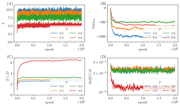
We can draw mutant phenotypes to be correlated with the phenotype of a parent, which is chosen with probability proportional to its abundance for each epoch. Given the parent phenotype—the vectors and —we draw a mutant phenotype and which has elementwise Pearson correlation with the parent phenotype. We also enforce elementwise correlation between and . In Figure 13 we show numerical results from this process. The trends are similar to what we observe when we vary in the linearized model and, importantly, show that there is still a Red Queen steady state across a range of , with the phase qualitatively similar to the phase studied in depth. Of particular phenomenological interest is the dependence of on , which displays a nonmonotonicity. We deliberately stay away from the limit , which is left for future work as additional subtleties arise.
Appendix C Relation between CR and linearized models
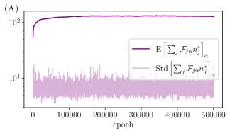
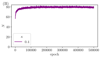
We here connect the CR model to the linearized model, which we have argued captures the behavior of the CR model and is easier to analyze. The linearization of as a function of the is justified when the mean of over (weighted by the ) is larger than its variations. In Figure 14A we show that this condition is met in the Red Queen steady state for . Figure 14B shows that the total consumer population is roughly constant in evolutionary time, which motivates a description in terms of fractional abundances for the linearized model. We carry out an expansion which allows us to separate out general fitness and interaction contributions to each strain’s growth rate.
In the Red Queen steady state the means of and are greater than due to evolutionary conditioning—for example in Figure 3A, the plot for shows that the mean of plateaus at . The mean of is smaller than that of but still larger than . If we define and , then we have . Defining , we can Taylor expand the resource abundances, yielding
| (30) |
where our definition of ensures that . If we approximate this expansion as an equality, at the fixed point the condition on the extant strains that their growth rates vanish becomes
| (31a) | ||||
| (31b) | ||||
where we have similarly defined and so that the average of over (weighted by ) vanishes. This form allows us to separate out the general fitness and interaction pieces in the growth rate of each strain. On the right hand side of Equation 31b, the first term contains the general fitnesses and is proportional to . The second term is the contribution to the growth rate of strain from the ecological interactions, and the last three terms are -independent and constitute an effective Lagrange multiplier that keeps roughly constant when .
In the assembled community, and the and have width and respectively. Therefore the width of the general fitness term scales as and the width of the interaction piece scales as . Since in an assembled community for sufficiently large , with each of the being , the distribution of general fitnesses is a factor of wider than the distribution of drives. Since and are in order to make the majority of entries in and positive, the general fitnesses dominate in the assembled community. However when the community evolves, the vectors elongate in the direction of the supply vector . As they push into their gaussian tail, they decrease the width of the distribution of extant , which is governed by the variations of the vectors in the direction parallel to . However the width of the extant drive distribution does not decrease and this allows the distributions of general fitnesses and growth rates from ecological interactions to attain comparable widths in an evolved community with (Section II.2).
Appendix D Algorithm to find fixed point
Integrating the ecological dynamics to find their stable fixed point is too slow to observe many of the features of the long-term evolution of interest. In order to probe longer evolutionary trajectories, we have used a heuristic method to find the fixed point; we then check that it is stable and cannot be invaded by any of the extinct strains. Below we describe the algorithm for the linearized and LV models, and a modification of the algorithm for the CR model. For the LV and linearized models, given an interaction matrix, the procedure can be modified to include selective differences by adding to the th row of : for ease of notation we refer to this effective interaction matrix simply as . The main challenge is to find the set of strains in the community that has nonzero abundance at the stable uninvadable fixed point. We accomplish this with an iterative method that converges most of the time.
-
1.
Initialize as the set of all strains in the community (including the new invader) and initialize the extinct set as an empty set. is the submatrix of interactions for the extant strains, and therefore contains the rows and columns corresponding to strains in .
-
2.
Invert to find a fixed point of the dynamics via and which fixes . In general some of the will be negative. Remove the set from and add it to .
-
3.
Calculate the invasion fitnesses of each strain in as . Transfer the set of strains that could invsade, , from to .
-
4.
Iterate steps and until convergence to sets and such that for all and for all .
One can then check stability of the final fixed point by computing the Jacobian of the dynamical equation. The vast majority of the time, the fixed point found in this way is stable.
When the algorithm does not converge within iterations, we stop adding extinct strains with positive invasion fitnesses back into the community, and thereby converge to a fixed point with positive abundances, which is invadable by some of the strains that were declared extinct. This adjustment is most often deployed when and have similar sizes at the fixed point, which can happen for an initial assembled community with large , or for the evolved state with small where is small and each invader can cause extinctions. In these cases the iterative algorithm does not converge reliably. However for small perturbations to the community, as in the case of primary interest, is much smaller than and the algorithm converges rapidly. Results from the error-prone regimes of evolution do not play a substantial part in any of our conclusions.
In the CR model, one cannot simply invert a matrix to find the fixed point for a subset of strains due to the nonlinearity in the interactions. Therefore we use a numerical solver to find the fixed point for a given —the rest of the algorithm is the same as in the linearized and LV cases.
Appendix E LV evolution across range of
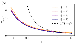
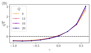
As in the linearized model, the LV model (shown in Figure 15 for ) exhibits a Red Queen steady state in which is less than its maximal value in an assembled community, , independent of , as reviewed in Appendix F. The gap between and diverges as , reflecting the fact that the fragility is numerically larger for , and so it drives an average of one strain extinct per invasion for farther from . For (as in these simulations) changes sign at , at which we have a quantitative understanding of the Red Queen phase (Section IV.3). As in the linearized model, we expect weak dependence of on , and for gaussian with large .
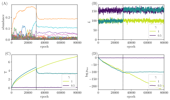
In the oligarch phase, for with for , there are strains that grow to comprise an fraction of the population, and continually increases with the community becoming harder and harder to invade. The width of the crossover between these two phases appears to sharpen for increasing (not shown), indicating a sharp transition in the high-diversity limit . The oligarch phase is not a steady state and runs away to arbitrarily large values, but remains roughly constant, and it is this that is plotted as for in Figure 15A.
The rate of increase of jumps discontinuously up from zero through the transition. This discontinuity suggests a first order transition, motivating our investigation of hysteresis around the critical . One can start the evolution with , and, after some period of time, reduce to below for the newly invading strains. Figure 16A shows strain abundance dynamics during such a “quench.” Here for the first epochs of evolution, after which the invading strains start to enter the community with . The strains into which an fraction of the community have condensed start to decrease in abundance, but instead of going extinct and turning over, they reach an apparent steady state in which they fluctuate around their still- mean values. This behavior becomes rarer as the post-quench is decreased, indicating a region of phase coexistence around . Figures 16B–D show the dynamics of , and through this process, compared with the behaviors for constant throughout the evolution and constant . If one looks only at , the hysteresis is not apparent, with the post-quench similar to for a community that has always had . Is it possible that, as for , the fragility only depends on but not the abundance distribution? If so, the fragility could set in steady state with little dependence on the history.
In contrast to , and show clearly that the post-quench steady state is significantly different from a Red Queen state that has been evolving with from its beginning. This post-quench steady state displays properties of both the oligarch phase and the Red Queen phase, and may therefore be a useful route to better understand the oligarch phase.
Appendix F Cavity calculation for assembled community
Here we carry out the static cavity calculation for a top-down assembled community in the linearized model: our results and approach are similar to that of ref. Blumenthal et al. [2024]. An analogous calculation for the LV model proceeds in a similar manner Bunin [2017], Pearce et al. [2020], Opper and Diederich [1992], and we summarize it at the end of this section. We consider a large community of strains at its fixed point, and add in another strain and resource, treating these as a small perturbation and then enforcing self-consistency between the statistics of this newly added strain and resource and the rest of the community. We will use the convention that repeated indices are summed over, unless otherwise stated.
Linearized model: The strains obey the dynamical equation
| (32) |
for , where for and with . Defining resources , the fixed point abundances satisfy
| (33) |
where tildes indicate the fixed point values prior to adding a new strain and resource. Now we add in a new strain and resource with fixed point abundances and respectively. Defining quantities and , we have
| (34) |
If we define “local susceptibilities” and , then the changes in and are and . (Here repeated indices are not summed.)
Assuming self-averaging (distributions concentrating around their mean for large systems), the new strain and resource abundances are
| (35) |
where and are “global ” susceptibilities.
Since and are weighted sums of the and matrix elements respectively, they are gaussian distributed with mean . We will denote their variances as and respectively. Let us take the to be gaussian distributed with mean and variance , and define and . We can now write self-consistency conditions for the variables , , , and , which require that the distributions of the added strain and resource abundances are the same as the distributions in the original community: in other words, Equation 35 is true for all strains, not just the cavity strain. Defining partial moments
| (36) |
our self-consistency conditions are
| (37a) | ||||
| (37b) | ||||
| (37c) | ||||
| (37d) | ||||
| (37e) | ||||
These equations can be reduced to
| (38a) | ||||
| (38b) | ||||
| (38c) | ||||
along with an equation for alone:
| (39) |
A solution to these equations give us the distributions of the strain and resource abundances in the community, as well as the susceptibilities and , and the scaled Lagrange multiplier . This mean field solution is expected to describe the unique stable uninvadable fixed point as long as it is stable: in particular to any small random perturbation on each of the strains’ growth rates.
To look at the nonlinear instability that signals the breakdown of the mean field theory, we add a random field to each of the biases and look at the change in the bias of strain . We find that
| (40) |
where the sum is over both and . Then in evaluating the mean square of both sides of this equation we have
| (41) |
Assuming that the strains are statistically identical, we can drop the strain indices to get
| (42a) | ||||
| (42b) | ||||
where we have defined the fragility as the factor relating the variance of the random fields to the sum of the squared changes in abundances that these produce. Since and in the mean field solution, we can write the fragility in terms of as
| (43) |
An instability signaling a phase transition occurs when the fragility diverges, at . We could have (more naturally) defined the fragility as the response of the strain abundances to adding a random field to the resource fields , but the form of divergence at the phase transition is the same in both cases (and in LV model, only the fragility we use here is defined). The location of the divergence implies that the number of surviving strains is at the transition. Substituting this relation into Equation 39 tells us that is the solution to
| (44) |
For , the solution to this equation is and . For , we have and , meaning that and . The reciprocal of gives the invasion probability of the saturated community by an independent invader. The scaling of and with and is reflected in the scaling forms of and in the Red Queen steady state.
Note that the linear susceptibility diverges when . The nonlinear instability occurs for lower than the linear instability for , meaning that the cavity solution becomes invalid before it displays a linear instability. The nonlinear and linear instabilities occur in the same place for , marking the onset of a “shielded” phase when Tikhonov and Monasson [2017]. With , diverges for , indicating the marginality of the shielded phase which occurs only for , .
LV model: We now summarize the cavity calculation for the LV model. In this case the cavity method yields, for the fixed point abundance of the cavity strain,
| (45) |
where , and . Note the similarity with the expression from the linearized model
| (46) |
(a consequence of Equations 35 and 38) if one identifies with , with and with , which account for the integrated-out resources as well as the factor of between the LV and linearized models.
The self consistency equations for the LV model with gaussian distributed of variance , for unknowns , and , are then
| (47a) | ||||
| (47b) | ||||
| (47c) | ||||
where, as before, . These equations can be reduced to
| (48) | |||
| (49) |
along with an equation for alone:
| (50) |
The fragility can be calculated from local susceptibility in terms of :
| (51) |
implying a divergence of at .
Appendix G Exponential distribution of general fitnesses
In order to analyze the transient behavior of as (the local scale of the distribution) decreases during the evolutionary transient, it is useful to investigate the behavior of the assembled community with an exponential distribution of positive given by . We define the variable . The self consistency conditions then deal with the distribution of , which is
| (52) |
where is the standard normal CDF and is the variance of the drives in the assembled community. If we define partial moments
| (53) |
then the self consistency conditions can be written down in a similar fashion to those for the gaussian in Equation 37. For the LV model, these conditions are
| (54) | ||||
| (55) | ||||
| (56) |
For large , the lower limit of the exponential does not matter and the distribution is roughly an unbounded exponential. Therefore we have
| (57) |
which allows us to write the self consistency conditions just in terms of the number of extant strains , regardless of and the normalization of :
| (58) | ||||
| (59) | ||||
| (60) |
In the large- regime, we therefore have , implying that to leading order in , the diversity is given by . A similar analysis in the linearized model yields .
As discussed in Section IV.5, the analysis of the exponential also describes the steady-state behavior for decaying faster than exponentially, and large. In that case, is a function of and the distribution of has pushed far enough into the tail of to look locally exponential around .
Note that and diverge for sufficiently large whether the critical , denoted , is proportional to—with an factor— in the LV model and in the linearized model. This is because, as increases, the maximum —given by and in the LV and linearized models respectively—becomes smaller than or respectively, and so cannot diverge. Therefore for an exponential , sufficiently large eliminates the instability of an assembled community.
For understanding the evolutionary transients in models with faster-than-exponential tails (Section IV.5), it is important to note that for , as more strains are added, continues to increase without the community otherwise changing.
Appendix H Dynamical cavity analysis in simplest case
Here we carry out the dynamical cavity analysis for the evolutionary steady state of the LV model with , . In particular we calculate the temporal correlation function of the cavity strain in Equation 10 and derive self-consistency conditions to find the statistical properties of the evolution of strain abundances. Throughout, we suppress the index of the cavity strain.
Solution for correlation function: Because of the absorbing boundary condition at , we can use the solution of the Ornstein Uhlenbeck process (Equation 11) together with the method of images to write down the distribution of given that it started at some initial value at invasion time . For simplicity we set : integrating the correlation function over —as we will later do—is the same as integrating over . We use the fact that, for , we have . Therefore we can write the distribution of conditioned on as
| (61) |
where we have used the notation to denote the probability density with an absorbing boundary condition at : the integral of over is the survival probability of the strain as a function of time . We calculate the expectation over the joint distribution . We then integrate over all times and over all distributed according to
| (62) |
where is the standard deviation of the incoming drive distribution, and is the rate of attempted invasions. in our case since time is in units of successful invasions, and so each invader has probability of successfully invading. The integrals over and correspond to summing over all the strains in the community and can be done exactly, yielding
| (63a) | ||||
| (63b) | ||||
We now assert that the dynamics of the cavity drive are the same as those of the drives in the community. Since the cavity drive can fluctuate in sign, its correlation function is , from an unconditioned Ornstein Uhlenbeck process at stationarity. Equating our two expressions for gives
| (64) |
We can get another self-consistency condition by enforcing . Note that , where the expectation is taken with an absorbing boundary condition at . Integrating this expression over the past and over the half-gaussian distribution of starting positions (as before) gives .
The number of strains in steady state, , is determined by the fact that the survival probability up to time is . Integrating over all past times and over the distribution of gives . Now we have two self-consistency conditions for and , along with an equation for :
| (65) | ||||
| (66) | ||||
| (67) |
We can solve these equations in terms of . The most easily testable prediction from numerics is
| (68) |
which agrees well with numerics for across a range of (Figure 10A). We also find that , and where , implying that . Therefore the theory prediction for the correlation function of the cavity drive is
| (69) |
As stated previously, since this makes the integral of the half-gaussian incoming drive distribution (and therefore the rate of incoming strains) equal to .
Lifetime distribution: The distribution of strain lifetimes can be computed using known results from the theory of Ornstein Uhlenbeck (OU) processes—which can also be derived from the method of images. A useful result Ricciardi and Sato [1988] is that the distribution of survival times for an OU process starting at position and ending when it hits the origin is
| (70) |
We can then integrate over the distribution
| (71) |
We obtain , as quoted in Equation 14.
Abundance distribution: The steady state distribution of abundances can also be computed from our self consistent solution. The abundance distribution obeys a Fokker Planck equation (with the appropriate boundary conditions) that captures the dynamics of the drives from Equation 11 and includes a source term for incoming invaders. Therefore in the steady state, the condition for stationarity of the distribution is
| (72) |
with boundary conditions . Equation 72 contains effects of the systematic and random parts in as well as the input from invading strains.
If we change variables to and so that , we find that the number density of the rescaled abundances obeys the -independent differential equation
| (73) |
with . The solution to this equation with boundary conditions , is plotted in Figure 9 as the theoretical prediction for the distribution of scaled abundances in the evolved community.
Appendix I Fluctuations in steady state:
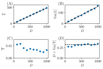
Figures 17A and B show that in the Red Queen steady state for the linearized model, fluctuates around a mean value which is proportional to , with fluctuations that scale with . This scaling is consistent with expectations from the finite fragility of the Red Queen steady state—with evolutionary perturbations to the community not causing large changes and fluctuations therefore down by a factor of . Figures 17C and D show the same statistics for . We expect to be but is anomalously small in simulations (since ), and it is possible that the coefficient of its part is zero, with a —or some other—correction showing up in numerics. For , we know that in the limit , , (which reduces to the Lotka-Volterra model), as well as when , since in the latter case becomes nonpositive and asymptotes to from below. It is therefore possible that for intermediate as well, but our results are inconclusive. Note that fluctuations in have size as expected.
Appendix J Evolutionary transients with
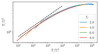
In Section IV.5 we discussed the transient behavior of the evolution as the distribution of extant pushes into the tail of . For a gaussian distribution of the , we expect that during the transient,
| (74) |
In Figure 18 we find that this prediction agrees well with numerics for as a function of evolutionary time, and the collapse of the curves scaled by verifies the predictions. The curves collapse even for , beyond which the cavity analysis would naively predict that the mean strain lifetime diverges. The data indicate that, in agreement with observation in Figure 5C, for our choice of parameters, the simulations with have not yet reached their steady state by the end of epochs. The dynamics of during the transient (not shown) are less well-fit by a simple power law since varies over a smaller range and has a larger constant correction.
Appendix K Correlations and lifetimes for nonzero and
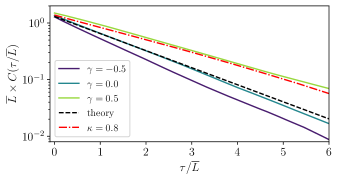
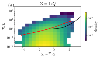
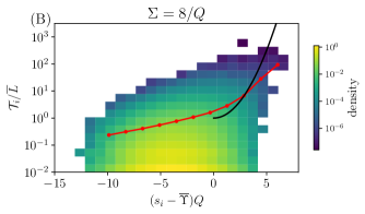
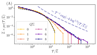
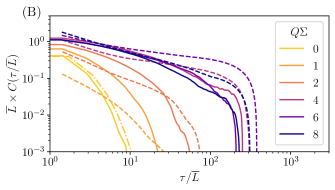
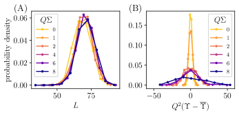
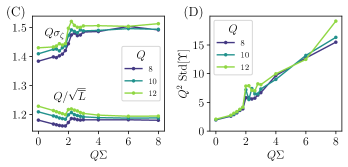
Here we examine the lifetime distribution, and the correlation function in the LV model for various with , and for gaussian with various , restricting to . We find that in all cases—even when the cavity analysis suggests otherwise (Section IV.5)—a steady state appears to obtain in numerics, and the lifetime distribution decays sufficient rapidly that the relation between the average strain lifetime and the average diversity holds.
Nonzero with : In Figure 19 we show for the LV model, with time rescaled by the average strain lifetime, equal to . Defining rescaled time , we see that decays exponentially for large , with the rate of this exponential depending on . Larger results in slower turnover and slower decay, presumably because with positive , invading strains are likely to increase the abundance of already-abundant strains, which therefore decay to extinction more slowly. Before the exponential regime it appears that for , decays slightly faster for small than for large , with the opposite trend for .
Nonzero with : In the LV model, due to the interactions being (instead of in the linearized model), the natural scale for the width of the extant distribution at steady state is , rather than . We therefore consider in the following analysis.
For , subtleties arise for gaussian as discussed in Section IV.5. For less than some crossover scale , is predicted to decay as a -dependent power law, while for (or for broader-than-gaussian ) one naively expects that large- strains cause to diverge, disallowing a steady state. However in contrast to this expectation, we find in numerics that a seemingly well-behaved steady state occurs even for large .
In order to understand this behavior it is useful to examine deviations from the cavity analysis exhibited by our numerics. As discussed in Section IV.5, extinction for large requires a rare fluctuation of away from zero (its mean) by an amount . If the stochastic process has a gaussian steady state even out into the rare tails of large negative , the rate of extinction (and therefore inverse lifetime) will be roughly , where is the variance of the stationary state distribution of . Figure 20 shows the joint distribution of and , and compares the mean lifetime for a given , denoted , to the predicted inverse-gaussian-large dependence. The numerics show a slower increase of with than suggested by a gaussian steady state, indicating wider fluctuations of and shorter lifetimes.
These shorter-than-expected lifetimes can also be seen directly from . Under the gaussian cavity assumption, strains which last for time will have typical general fitness . If , this yields an estimate for the large- decay of : for , we have , while for gaussian we have, at asymptotically long times,
| (75) |
which yields a finite only for , i.e. . At intermediate times, especially for larger , is expected to decay as with , due to the roughly exponential decay of (with slope ) near .
In Figure 21A is plotted on a log-log scale for gaussian with various . As goes from to , increases modestly from to , and barely changes (Figures 22A and C). Even for , which is less than , the decay of is considerably faster than the predicted . For the difference between numerics and cavity analysis is even larger: appears to saturate at in contrast to the predicted for , and is not well fit by the intermediate- transient either (Figure 21A). Thus something is making the rare fluctuations to large negative —assuming the basic cavity structure in terms of is still valid—much larger than gaussian.
Given the difference between naive expectations and numerics for , we investigate whether these differences carry over to the correlation function, , which, as discussed in Section IV.5, is determined by strains that survive for at least time . is plotted in Figure 21B for gaussian with the same range of between and . With the joint distribution of and , and approximating the contribution to of a strain with by , can be estimated from the observed (Equation 20). The result of this estimation is shown in Figure 21B along with the empirically calculated , and we find rough agreement.
As discussed in Section IV.5, a possible source of the discrepancy between naive cavity analysis and numerics is the emergence of long-tailed memory kernels that increase the rate of extinction by allowing anomalously long-lasting negative . Such dynamics could drive strains with large extinct at a higher rate than the naive “barrier-crossing” estimate. But as long as the is a stationary gaussian process, this cannot happen: the correlations between and the typically-small at the invasion time can only decrease the probability of a large deviation. Instead, a more viable scenario is that the large- limit is subtle with large deviations from the gaussian Ansatz of the statistics making extinction events of large strains much less unlikely, as seen in Figure 20.
In general, one does not expect that the limits of large and behavior in the tails of distributions will commute: the central limit theorem is only for the non-too-rare center of the distribution. Likewise, the long-time limit and large limit need not commute. Concretely, if large fluctuations that drive extinctions are only exponentially rare in , and hence lifetimes “only” exponentially long in , would decay roughly as a power of even for very large where the distribution of extant is close to exponential. This behavior is roughly consistent with the apparent power-law decay in this regime (Figure 21A). Exponential—rather than gaussian—tails often occur, for example if the rare events that drive extinctions result from the sum of effects of a series of roughly independent events. Thus this putative resolution of the apparent paradox may well be viable.
Another effect that could cause extinctions is large fluctuations in , particularly for exponential , which plays a key role in the behavior for large . With exponential (in contrast to ) there is no special value of in steady state. Instead there is a special value of for which a steady state occurs, equal to the steady-state for all in the limit of large (Section IV.5). Since any in an exponential tail is equivalent (conditioned on invasion of strains) there are likely to be at least diffusive—and hence unbounded—fluctuations in . Upwards fluctuations in would eventually drive extinctions of strains that had anomalously large at their invasion time. Additionally, persistent large- strains will themselves cause substantial increases in , perhaps providing sufficient feedback for these to limit their own lifetimes.
The fluctuations in about the steady state for gaussian can be estimated by noting that in the LV model, an invader changes by an amount of order , the typical amount needed to keep for the random changes in caused by the invasion (Section IV.2). Combining these diffusive fluctuations with the linear deterministic push towards (which can be seen by expanding Equation 23 for near ) yields a prediction: . Simulations for modest in Figure 22 show that while the distribution of in steady state depends only weakly on , the distribution of in steady state appears consistent with this dependence on . We expect that the diffusion coefficient of would increase—and perhaps diverge—for large , due to long-time correlations of the fluctuations in and hence in . In order to play a role in the extinctions of strains with large , fluctuations of would have to be larger than expected by a factor of , and would likely need to have non-gaussian tails as well. While we have not explored the tails, Figures 22B and D indeed show increased fluctuations in as a function of increasing , with a sharp increase as passes through at which the naive analysis predicts a divergence of . For larger , the dependence of on becomes stronger, perhaps indicating a crossover to a regime with the fluctuations scaling as and thus comparable to .
At this point it is unclear what kind of non-gaussian fluctuations, or other subtleties of large but finite , cause the persistence of a Red Queen steady state even when large ’s can occur. However our numerics indicate that the eco-evolutionary steady state obtains even for large with gaussian . Further investigation of is needed, but it is possible that a similar mechanism preserves the steady state there as well.
Appendix L Comparison with results of de Pirey and Bunin
Recent work of de Pirey and Bunin Arnoulx de Pirey and Bunin [2024] (dPB for short) has explored a Red Queen-like phase in a different context. dPB study ecological dynamics in a Lotka-Volterra model in the limit of small migration for each species, such that there is a clear separation between extant species which have substantial abundance, and species which would be extinct if not for the small migration. They find that if the diversity is high enough, the ecological dynamics are chaotic such that there are species which go nearly extinct before rising again to high abundance and rejoining the extant subset which is almost at a stable fixed point. Due to a separation of timescales arising from the very small migration rate (analogous to our separation of evolutionary and ecological timescales), the ecological dynamics consist of a series of almost-fixed points punctuated by changes that occur when a near-extinct species rises up to non-negligible abundance.
When a species transitions from near-extinct to extant, the process is similar to an independent invader joining the community, as the abundance of the invader can jump up to a nonzero value determined by its ecological interactions with the extant community. This entrance to the community causes a change in the biases of the other strains, which can drive low abundance strains out and produces a steady state in which low-abundance strains are depleted relative to the truncated gaussian distribution of the assembled community. Indeed dPB find that their distribution at steady state is not well approximated by a truncated gaussian, and the number of extant species at any given time is less than the total capacity of an assembled community.
However, in the model studied by dPB, the steady state abundance distribution does not vanish at zero abundance, in contrast to our evolved communities. This is because when a species goes from extant to nearly-extinct, its probability of rejoining the extant community due to an ecological fluctuation is a decreasing function of time as ecological fluctuations drive its abundance farther from the boundary between extant and near-extinct. Therefore the boundary condition at zero abundance is not an absorbing one but rather a permeable boundary where species that hit zero abundance can be resurrected by a small change in the community and come back into the community soon after their extinction. dPB are able to write dynamical mean field equations for the abundance dynamics and solve these equations numerically to get the steady state abundance distribution. Our case turns out to be simpler in this respect since with evolutionary dynamics the extinction boundary is strictly absorbing which, fortuitously, makes the self-consistent correlations simple and enables an exact solution, with the equation satisfied by the abundance distribution reduced to a boundary value problem (Equation 73) that can be solved numerically (Figure 9).
References
- Sunagawa et al. [2015] Shinichi Sunagawa, Luis Pedro Coelho, Samuel Chaffron, Jens Roat Kultima, Karine Labadie, Guillem Salazar, Bardya Djahanschiri, Georg Zeller, Daniel R Mende, Adriana Alberti, et al. Structure and function of the global ocean microbiome. Science, 348(6237):1261359, 2015.
- hum [2012] A framework for human microbiome research. Nature, 486(7402):215–221, 2012.
- Fierer [2017] Noah Fierer. Embracing the unknown: disentangling the complexities of the soil microbiome. Nature Reviews Microbiology, 15(10):579–590, 2017.
- Kashtan et al. [2014] Nadav Kashtan, Sara E Roggensack, Sébastien Rodrigue, Jessie W Thompson, Steven J Biller, Allison Coe, Huiming Ding, Pekka Marttinen, Rex R Malmstrom, Roman Stocker, et al. Single-cell genomics reveals hundreds of coexisting subpopulations in wild prochlorococcus. Science, 344(6182):416–420, 2014.
- Rosen et al. [2015] Michael J Rosen, Michelle Davison, Devaki Bhaya, and Daniel S Fisher. Fine-scale diversity and extensive recombination in a quasisexual bacterial population occupying a broad niche. Science, 348(6238):1019–1023, 2015.
- Rosenzweig et al. [1994] R Frank Rosenzweig, RR Sharp, David S Treves, and Julian Adams. Microbial evolution in a simple unstructured environment: genetic differentiation in escherichia coli. Genetics, 137(4):903–917, 1994.
- Friesen et al. [2004] Maren L Friesen, Gerda Saxer, Michael Travisano, and Michael Doebeli. Experimental evidence for sympatric ecological diversification due to frequency-dependent competition in escherichia coli. Evolution, 58(2):245–260, 2004.
- Maharjan et al. [2006] Ram Maharjan, Shona Seeto, Lucinda Notley-McRobb, and Thomas Ferenci. Clonal adaptive radiation in a constant environment. Science, 313(5786):514–517, 2006.
- Good et al. [2017] Benjamin H Good, Michael J McDonald, Jeffrey E Barrick, Richard E Lenski, and Michael M Desai. The dynamics of molecular evolution over 60,000 generations. Nature, 551(7678):45–50, 2017.
- Lenski [2017] Richard E Lenski. Experimental evolution and the dynamics of adaptation and genome evolution in microbial populations. The ISME journal, 11(10):2181–2194, 2017.
- Finkel and Kolter [1999] Steven E Finkel and Roberto Kolter. Evolution of microbial diversity during prolonged starvation. Proceedings of the National Academy of Sciences, 96(7):4023–4027, 1999.
- Ignacio-Espinoza et al. [2020] J Cesar Ignacio-Espinoza, Nathan A Ahlgren, and Jed A Fuhrman. Long-term stability and red queen-like strain dynamics in marine viruses. Nature Microbiology, 5(2):265–271, 2020.
- Marston et al. [2012] Marcia F Marston, Francis J Pierciey Jr, Alicia Shepard, Gary Gearin, Ji Qi, Chandri Yandava, Stephan C Schuster, Matthew R Henn, and Jennifer BH Martiny. Rapid diversification of coevolving marine synechococcus and a virus. Proceedings of the National Academy of Sciences, 109(12):4544–4549, 2012.
- Buckling and Rainey [2002] Angus Buckling and Paul B Rainey. Antagonistic coevolution between a bacterium and a bacteriophage. Proceedings of the Royal Society of London. Series B: Biological Sciences, 269(1494):931–936, 2002.
- Van Valen [1973] Leigh Van Valen. A new evolutionary law. Evolutionary Theory, 1:1, 1973.
- De Visser and Krug [2014] J Arjan GM De Visser and Joachim Krug. Empirical fitness landscapes and the predictability of evolution. Nature Reviews Genetics, 15(7):480–490, 2014.
- Fisher [2021] Daniel S Fisher. Inevitability of red queen evolution driven by organismic complexity and simple feedback via environmental modification. bioRxiv, pages 2021–09, 2021.
- Agarwala and Fisher [2019] Atish Agarwala and Daniel S Fisher. Adaptive walks on high-dimensional fitness landscapes and seascapes with distance-dependent statistics. Theoretical Population Biology, 130:13–49, 2019.
- Bunin [2017] Guy Bunin. Ecological communities with lotka-volterra dynamics. Physical Review E, 95(4):042414, 2017.
- Opper and Diederich [1992] Manfred Opper and Sigurd Diederich. Phase transition and 1/f noise in a game dynamical model. Physical Review Letters, 69(10):1616, 1992.
- Blumenthal et al. [2024] Emmy Blumenthal, Jason W Rocks, and Pankaj Mehta. Phase transition to chaos in complex ecosystems with nonreciprocal species-resource interactions. Physical Review Letters, 132(12):127401, 2024.
- Ros et al. [2023] Valentina Ros, Felix Roy, Giulio Biroli, Guy Bunin, and Ari M Turner. Generalized lotka-volterra equations with random, nonreciprocal interactions: The typical number of equilibria. Physical Review Letters, 130(25):257401, 2023.
- Pearce et al. [2020] Michael T Pearce, Atish Agarwala, and Daniel S Fisher. Stabilization of extensive fine-scale diversity by ecologically driven spatiotemporal chaos. Proceedings of the National Academy of Sciences, 117(25):14572–14583, 2020.
- Xue and Goldenfeld [2017] Chi Xue and Nigel Goldenfeld. Coevolution maintains diversity in the stochastic “kill the winner” model. Physical Review Letters, 119(26):268101, 2017.
- Huisman et al. [2001] Jef Huisman, Anna M Johansson, Eelke O Folmer, and Franz J Weissing. Towards a solution of the plankton paradox: the importance of physiology and life history. Ecology Letters, 4(5):408–411, 2001.
- Yan et al. [2019] Le Yan, Richard A Neher, and Boris I Shraiman. Phylodynamic theory of persistence, extinction and speciation of rapidly adapting pathogens. Elife, 8:e44205, 2019.
- Armstrong and McGehee [1980] Robert A Armstrong and Richard McGehee. Competitive exclusion. The American Naturalist, 115(2):151–170, 1980.
- Shoresh et al. [2008] Noam Shoresh, Matthew Hegreness, and Roy Kishony. Evolution exacerbates the paradox of the plankton. Proceedings of the National Academy of Sciences, 105(34):12365–12369, 2008.
- Schippers et al. [2001] Peter Schippers, Antonie M Verschoor, Matthijs Vos, and Wolf M Mooij. Does “supersaturated coexistence” resolve the “paradox of the plankton”? Ecology letters, 4(5):404–407, 2001.
- Doebeli and Ispolatov [2010] Michael Doebeli and Iaroslav Ispolatov. Complexity and diversity. Science, 328(5977):494–497, 2010.
- Tikhonov and Monasson [2018] Mikhail Tikhonov and Remi Monasson. Innovation rather than improvement: A solvable high-dimensional model highlights the limitations of scalar fitness. Journal of Statistical Physics, 172:74–104, 2018.
- Serván and Allesina [2021] Carlos A Serván and Stefano Allesina. Tractable models of ecological assembly. Ecology Letters, 24(5):1029–1037, 2021.
- Capitán et al. [2009] José A Capitán, José A Cuesta, and Jordi Bascompte. Statistical mechanics of ecosystem assembly. Physical Review Letters, 103(16):168101, 2009.
- Altieri et al. [2021] Ada Altieri, Felix Roy, Chiara Cammarota, and Giulio Biroli. Properties of equilibria and glassy phases of the random lotka-volterra model with demographic noise. Physical Review Letters, 126(25):258301, 2021.
- Tikhonov and Monasson [2017] Mikhail Tikhonov and Remi Monasson. Collective phase in resource competition in a highly diverse ecosystem. Physical Review Letters, 118(4):048103, 2017.
- Cui et al. [2020] Wenping Cui, Robert Marsland III, and Pankaj Mehta. Effect of resource dynamics on species packing in diverse ecosystems. Physical Review Letters, 125(4):048101, 2020.
- Biroli et al. [2018] Giulio Biroli, Guy Bunin, and Chiara Cammarota. Marginally stable equilibria in critical ecosystems. New Journal of Physics, 20(8):083051, 2018.
- Marsland III et al. [2020] Robert Marsland III, Wenping Cui, and Pankaj Mehta. The minimum environmental perturbation principle: A new perspective on niche theory. The American Naturalist, 196(3):291–305, 2020.
- Bonachela et al. [2017] Juan A Bonachela, Meike T Wortel, and Nils Chr Stenseth. Eco-evolutionary red queen dynamics regulate biodiversity in a metabolite-driven microbial system. Scientific Reports, 7(1):17655, 2017.
- Law et al. [1997] Richard Law, Paul Marrow, and Ulf Dieckmann. On evolution under asymmetric competition. Evolutionary Ecology, 11:485–501, 1997.
- Nordbotten and Stenseth [2016] Jan Martin Nordbotten and Nils C Stenseth. Asymmetric ecological conditions favor red-queen type of continued evolution over stasis. Proceedings of the National Academy of Sciences, 113(7):1847–1852, 2016.
- May [1972] Robert M May. Will a large complex system be stable? Nature, 238(5364):413–414, 1972.
- Mahadevan et al. [2023] Aditya Mahadevan, Michael T Pearce, and Daniel S Fisher. Spatiotemporal ecological chaos enables gradual evolutionary diversification without niches or tradeoffs. Elife, 12:e82734, 2023.
- Posfai et al. [2017] Anna Posfai, Thibaud Taillefumier, and Ned S Wingreen. Metabolic trade-offs promote diversity in a model ecosystem. Physical Review Letters, 118(2):028103, 2017.
- Caetano et al. [2021] Rodrigo Caetano, Yaroslav Ispolatov, and Michael Doebeli. Evolution of diversity in metabolic strategies. Elife, 10:e67764, 2021.
- Daly et al. [2018] Aisling J Daly, Jan M Baetens, and Bernard De Baets. Ecological diversity: measuring the unmeasurable. Mathematics, 6(7):119, 2018.
- Vrins [2018] Frédéric Vrins. Sampling the multivariate standard normal distribution under a weighted sum constraint. Risks, 6(3):64, 2018.
- Diederich and Opper [1989] Sigurd Diederich and Manfred Opper. Replicators with random interactions: A solvable model. Physical Review A, 39(8):4333, 1989.
- Roy et al. [2019] Felix Roy, Giulio Biroli, Guy Bunin, and Chiara Cammarota. Numerical implementation of dynamical mean field theory for disordered systems: Application to the lotka–volterra model of ecosystems. Journal of Physics A: Mathematical and Theoretical, 52(48):484001, 2019.
- Cugliandolo et al. [1997] Leticia F Cugliandolo, Jorge Kurchan, Pierre Le Doussal, and Luca Peliti. Glassy behaviour in disordered systems with nonrelaxational dynamics. Physical Review Letters, 78(2):350, 1997.
- Arnoulx de Pirey and Bunin [2024] Thibaut Arnoulx de Pirey and Guy Bunin. Many-species ecological fluctuations as a jump process from the brink of extinction. Physical Review X, 14(1):011037, 2024.
- Bonsma-Fisher and Goyal [2023] Madeleine Bonsma-Fisher and Sidhartha Goyal. Dynamics of immune memory and learning in bacterial communities. Elife, 12:e81692, 2023.
- Marchi et al. [2021] Jacopo Marchi, Michael Lässig, Aleksandra M Walczak, and Thierry Mora. Antigenic waves of virus-immune coevolution. Proceedings of the National Academy of Sciences, 118(27):e2103398118, 2021.
- Goyal et al. [2022] Akshit Goyal, Leonora S Bittleston, Gabriel E Leventhal, Lu Lu, and Otto X Cordero. Interactions between strains govern the eco-evolutionary dynamics of microbial communities. Elife, 11:e74987, 2022.
- Yoshida et al. [2007] Takehito Yoshida, Stephen P Ellner, Laura E Jones, Brendan J M Bohannan, Richard E Lenski, and Nelson G Hairston Jr. Cryptic population dynamics: rapid evolution masks trophic interactions. PLoS Biology, 5(9):e235, 2007.
- Valles-Colomer et al. [2023] Mireia Valles-Colomer, Aitor Blanco-Míguez, Paolo Manghi, Francesco Asnicar, Leonard Dubois, Davide Golzato, Federica Armanini, Fabio Cumbo, Kun D Huang, Serena Manara, et al. The person-to-person transmission landscape of the gut and oral microbiomes. Nature, 614(7946):125–135, 2023.
- Zhou et al. [2020] Wei Zhou, Michelle Spoto, Rachel Hardy, Changhui Guan, Elizabeth Fleming, Peter J Larson, Joseph S Brown, and Julia Oh. Host-specific evolutionary and transmission dynamics shape the functional diversification of staphylococcus epidermidis in human skin. Cell, 180(3):454–470, 2020.
- Martin-Platero et al. [2018] Antonio M Martin-Platero, Brian Cleary, Kathryn Kauffman, Sarah P Preheim, Dennis J McGillicuddy, Eric J Alm, and Martin F Polz. High resolution time series reveals cohesive but short-lived communities in coastal plankton. Nature Communications, 9(1):266, 2018.
- Ricciardi and Sato [1988] Luigi M Ricciardi and Shunsuke Sato. First-passage-time density and moments of the ornstein-uhlenbeck process. Journal of Applied Probability, 25(1):43–57, 1988.