Autoencoder Enhanced Realised GARCH on Volatility Forecasting
Abstract
Realised volatility has become increasingly prominent in volatility forecasting due to its ability to capture intraday price fluctuations. With a growing variety of realised volatility estimators, each with unique advantages and limitations, selecting an optimal estimator may introduce challenges. In this thesis, aiming to synthesise the impact of various realised volatility measures on volatility forecasting, we propose an extension of the Realised GARCH model that incorporates an autoencoder-generated synthetic realised measure, combining the information from multiple realised measures in a nonlinear manner. Our proposed model extends existing linear methods, such as Principal Component Analysis and Independent Component Analysis, to reduce the dimensionality of realised measures. The empirical evaluation, conducted across four major stock markets from January 2000 to June 2022 and including the period of COVID-19, demonstrates both the feasibility of applying an autoencoder to synthesise volatility measures and the superior effectiveness of the proposed model in one-step-ahead rolling volatility forecasting. The model exhibits enhanced flexibility in parameter estimations across each rolling window, outperforming traditional linear approaches. These findings indicate that nonlinear dimension reduction offers further adaptability and flexibility in improving the synthetic realised measure, with promising implications for future volatility forecasting applications.
1 Introduction
1.1 Background
Financial volatility modelling and forecasting are crucial tools for understanding and managing risk in financial markets. The 2008 Global Financial Crisis (GFC) and the COVID-19 pandemic are stark reminders of the devastating consequences of inadequate volatility assessment. During the GFC, flawed volatility models failed to capture the mounting risk within the subprime mortgage market, leading to underestimation of potential losses, institutional failures and widespread economic fallout. Similarly, during COVID-19, the unprecedented volatility drove sharp and extreme price fluctuations in the stock market, resulting in significant losses for investors. These events clearly demonstrate the important link between financial market volatility and the real economy. Effective volatility analysis provides valuable insights for financial institutions and policymakers, acting as a barometer for the vulnerability of financial markets and aiding in risk management and timely interventions. More importantly, advanced volatility forecasting can detect early warning signals, allowing stakeholders to anticipate potential shocks and deal with similar financial crises more effectively in the future. Given these roles in maintaining financial stability, accurate volatility forecasting is a meaningful topic in financial research.
One may ask why we do not focus on predicting returns directly to control outcomes. The challenge lies in the nature of financial returns, specifically of stocks, which are affected by many factors, such as the efficient market hypothesis and the random walk nature of price movement, both of which make predicting returns notoriously challenging (McAleer and Medeiros,, 2008). Financial volatility, on the other hand, exhibits more predictable behaviours, such as mean reversion, making it mathematically more feasible to forecast than returns (Poon and Granger,, 2003).
Another complexity is that volatility is a latent variable, it cannot be explicitly observed from a single piece of data (Andersen and Teräsvirta,, 2009). Although we can observe closing prices and changes, these are the results of volatility rather than direct measures of it. Volatility is not directly observable as it represents the underlying variability in a market’s returns over a period. To estimate this hidden volatility, we infer it from the known values, such as point-to-point returns. Daily squared returns are widely used in financial research as a proxy for volatility, approximating the latent volatility by reflecting the magnitude of price changes. However, the daily squared return is typically calculated at the end of a day using the closing price. They can reflect the volatility observed in the entire previous day, but cannot provide real-time information.
Extensive effort has been dedicated to finding good real-time estimates of current volatility. With the rapidly increasing availability of high-frequency transaction data across financial assets, researchers have developed a more accurate ex-post volatility estimator, realised volatility. The realised volatility calculated from high-frequency intraday returns captures price changes at very fine time scales, such as minute-by-minute or even seconds, providing a near real-time estimate of “true” volatility (Andersen and Teräsvirta,, 2009). Now, this measure is widely used as it offers a dynamic view of volatility in near real-time, offering a more immediate estimate of volatility than daily returns.
With these measures in place, researchers and practitioners also recognise that volatility has both persistence and heteroskedasticity features (Poon and Granger,, 2003; Engle,, 2004). To capture these characteristics, volatility measures are often integrated into advanced econometric models, such as Generalised Autoregressive Conditional Heteroskedasticity (GARCH) (Bollerslev,, 1986) and Realised GARCH models (Hansen et al.,, 2012), which employs squared returns and realised volatility, respectively, to account for the inherent latent and dynamic nature of volatility (Andersen and Teräsvirta,, 2009).
1.2 Research Question and Objective
With realised volatility becoming increasingly prevalent, numerous measures for realised volatility have been developed, such as Realised Variance, Realised Kernel, and Bipower Variation, et al. This variety leads to an initial research question: which realised volatility measure should be selected for volatility forecasting analysis? Naimoli et al., (2022) handle this by generating a synthetic realised measure from a range of candidate measures using linear combination techniques, including Principal Component Analysis and Independent Component Analysis, and incorporate them into the Realised GARCH model to improve the accuracy of volatility forecasting. Inspired by the idea of combining various measures into a single synthetic measure, and recognising the limitations of linear transformations, we propose to explore the potential benefits of a nonlinear combination for generating this synthetic measure. This leads to the final research question: does employing a nonlinear dimension reduction approach enhance the effectiveness of the synthetic realised volatility measure in Realised GARCH compared to linear methods?
Autoencoder, as a deep learning algorithm based on neural network architecture, has an outstanding ability for nonlinear dimension reduction and numerous applications in financial time series analysis. In this context, our research objective is designed to: develop a framework that uses nonlinear dimension reduction through an autoencoder to generate a synthetic realised volatility measure with essential information and incorporate it into Realised GARCH for volatility forecasting.
The primary contribution of this thesis lies in the novel use of autoencoder-based nonlinear dimension reduction to create a flexible synthetic measure. This enhanced measure enables Realised GARCH to achieve more adaptable parameter estimations at each forecasting step, ultimately improving volatility forecasting accuracy compared to linear methods.
1.3 Thesis Structure
The rest of this thesis is presented as follows: Chapter 2 reviews the relevant literature on volatility forecasting models, realised volatility measures, and dimension reduction techniques. Chapter 3 presents the essential knowledge of background models, along with the proposed framework and its parameter estimation method. Chapter 4 provides an empirical study of the proposed model, comparing in-sample estimates and out-of-sample forecasting performance against competing models. Chapter 5 summarises the conclusions, discusses limitations, and suggests future research directions.
2 Literature Review
2.1 GARCH Models and Realised Volatility
2.1.1 Introduction to GARCH Models
Since the groundbreaking paper of Engle, (1982), Autoregressive Conditional Heteroskedasticity (ARCH) offers a new perspective for understanding volatility. Bollerslev, (1986) further expands it to include the lagged conditional variance to predict future volatility, developing the Generalised ARCH (GARCH). Since their introduction, ARCH and GARCH have been recognised as foundational approaches to financial volatility modelling and are commonly used to describe and predict volatility. Specifically, GARCH uses squared daily returns as a proxy for the ex-post volatility. Let innovation in returns be written as , where represents an independent stochastic process with mean zero and unit variance, while the latent volatility evolves according to the specific model formula. This approach provides an unbiased estimate of volatility as . However, it is prone to noise from idiosyncratic errors , especially during periods of significant volatility changes (Andersen and Bollerslev,, 1998). This noise limits the model’s effectiveness in adjusting to new levels of volatility, highlighting the need for more efficient volatility measures based on high-frequency data (Hansen et al.,, 2012).
2.1.2 Realised Volatility Measures
As high-frequency financial data become increasingly available and standard in volatility forecasting. The latent volatility can be measured by analysing the variability of intraday squared returns based on high-frequency data, which provides more information than daily squared returns (Andersen et al.,, 2003). Therefore, Realised Variance (RV) was introduced by Andersen and Bollerslev, (1998), as a realised volatility measure, dramatically outperforming daily squared returns. In addition to RV, several more informative measures for volatility have been proposed, such as the Realised Kernel (RK) (Barndorff-Nielsen and Shephard,, 2002), and Bipower Variation (BV) (Barndorff-Nielsen,, 2004).
RV is calculated by summing the intraday squared returns, a method that has been extensively used for volatility measurement. However, high-frequency data based RV is contaminated by the market microstructure effect, such as discreteness of prices, bid-ask bounce and irregular trading, which introduce noise into the data. This noise arises because the microstructure effect is not reflective of actual price changes but from the mechanics of trading. As a result, using high-frequency data may lead to inaccurate volatility estimates as the observed fluctuations are affected by factors unrelated to “true” volatility. On the other hand, using low-frequency data may miss important volatility information from price changes. Therefore, RV faces the problem of deriving the appropriate frequency to balance the noise impact and the loss of information (Christensen and Podolskij,, 2007).
Barndorff-Nielsen and Shephard, (2002) focus on kernel-based estimators and design the class of RK. RK estimates the quadratic variation from high-frequency noisy data, similar to the sum-of-squares variance estimator. However, it combines the estimation of intraday volatility and kernel smoothing, resulting in robustness and efficiency in the presence of market frictions, therefore being more robust to microstructure noise (Barndorff-Nielsen et al., 2008a, ).
BV is introduced by Barndorff-Nielsen, (2004) as a realised volatility measure that effectively distinguishes between the continuous and jump components of price movements. Unlike RV, which captures both continuous price movements and rare price jumps, BV is designed to specifically capture the continuous component of the price process, calculated by summing the products of absolute returns over adjacent time intervals. The difference between RV and BV, known as the jump variation, provides an estimate of the jump component of volatility, capturing the effect of large and infrequent price changes which is a key element in volatility modelling (Barndorff-Nielsen,, 2004).
In addition, various other realised measures exist and serve as candidate measures in this thesis. Realised Semivariance (RSV), which divides RV into downside and upside, emphasises the magnitude of downside risk (Barndorff-Nielsen et al., 2008c, ). Median Realised Variance (MedRV) squares the median absolute return among three consecutive intraday returns, asymptotically avoiding the impact of a jump in the measure while reducing the sensitivity to the extreme return values caused by the microstructure effect within the trading day (Andersen et al.,, 2012). Two-scale Realised Kernel (TwoScale RK) proposed by Ikeda, (2015) is a bias-corrected realised kernel estimator, given by a particular convex combination of two RK estimators with different bandwidths.
Although some of the measures introduced above can partially mitigate the impact of microstructure, their reliance on high-frequency data still exposes them to microstructure noise (Christensen et al.,, 2017). Consequently, the techniques for smoothing out noise can also be used in realised volatility measures.
The subsampling approach introduced by Zhang et al., (2005) involves taking samples every 5 minutes, starting with the first observation, then the second, and so forth. Then averaging the results across those subgrids significantly decreases bias. The Parzen Weighted RK introduced by Barndorff-Nielsen et al., 2008b assigns varying weights to observations based on their distance from the centre of the sample, focusing on central and reducing noisy observations, thus dampening the influence of high-frequency noise.
2.1.3 Incorporating Realised Measures in GARCH Models
Based on the informative characteristics of the realised volatility measures, they provide significant improvements in modelling volatility compared to squared returns. These improvements have led researchers to incorporate realised measures directly into volatility models. Engle, (2002) includes a realised measure like RV in the GARCH framework (GARCH-X), effectively illustrating the feasibility of using RV in forecasting volatility. In the GARCH-X model, the high-frequency data-based realised measure is used as an exogenous variable (X).
Building on GARCH-X, Hansen et al., (2012) introduce the Realised GARCH model (RealGARCH), which addresses the gap by incorporating an explicit volatility explanation within the realised measure. RealGARCH adds a measurement equation, relating the observed realised volatility as a dependent variable on contemporaneous latent volatility. Watanabe, (2012) verifies the predictive likelihood improvement of RealGARCH over GARCH and GARCH-X models.
To extend RealGARCH further, Hansen and Huang, (2016) develop the Realised Exponential GARCH (RealEGARCH), allowing the incorporation of multiple realised volatility measures through multiple measurement equations. Compared with RealGARCH, an additional feature of the RealEGARCH model is the introduction of two leverage terms within both GARCH and measurement equations.
2.2 Linear Dimension Reduction
Given the numerous volatility measures proposed in the existing literature, one of the new questions is which realised measure should be selected in the model. Although RealEGARCH can incorporate multiple realised measures for volatility, this added additional flexibility is achieved at the price of a higher-dimensional problem (Naimoli et al.,, 2022).
To overcome the high-dimensional problem when considering multiple realised measures, dimension reduction can be employed as a solution. There are many famous linear dimensionality-reduced techniques, such as Principal Component Analysis (PCA) and Independent Component Analysis (ICA). PCA is a nonparametric method that is applied to reduce the dimensionality of the data while maintaining as much variability as possible. It was invented by Pearson, (1901) and further developed by Hotelling, (1933). Given the calculation of eigenvectors of the covariance matrix of the input data, PCA linearly transforms high-dimension inputs into low-dimension ones whose components are not correlated (Cao et al.,, 2003). In addition, these components are also ordered according to the variance, which means that the first principal component can explain the largest variance (Tahmasebi et al.,, 2020).
ICA is considered as an extension of PCA. Instead of focusing on optimising the covariance matrix of the data, ICA optimises higher-order statistics such as kurtosis (Tharwat,, 2021). ICA targets independent components and can extract statistically independent sources when the higher-order correlations are insignificant (Hyvärinen and Oja,, 2000). Hyvarinen, (1999) propose an algorithm of ICA called FastICA, which extracts the independent component by maximising non-Gaussianity. Later, ICA was generalised to a well-known method like PCA for feature extraction (Jang et al.,, 1999).
With the promotion of PCA and ICA, there are many applications of these techniques applied in Multivariate Factor GARCH. For PCA, such as Orthogonal-GARCH (Alexander,, 2001), Generalised Orthogonal-GARCH (Van Der Weide,, 2002), and conditionally uncorrelated component model (Fan et al.,, 2008). For ICA, it has been widely applied in financial econometrics, such as papers of Chen et al., (2007) and García-Ferrer et al., (2012), among others.
In order to overcome the problem of selecting the optimal set of realised volatility measures and integrating it in a univariate RealGARCH framework, Naimoli et al., (2022) propose an extension of RealGARCH with the use of PCA and ICA, respectively, denoted as PC-RealGARCH and IC-RealGARCH. By incorporating dimension reduction techniques, a synthetic realised volatility measure is generated from a wide range of candidate realised measures, and it is used to substitute a single realised measure in RealGARCH. The performance of PC-RealGARCH and IC-RealGARCH with a mixed realised measure leads to significant accuracy gains in tail risk forecasting (Naimoli et al.,, 2022).
2.3 Nonlinear Dimension Reduction
While PCA is widely used for dimension reduction, its linear structure may reduce its effectiveness in capturing the complexity of nonlinear data. In this case, nonlinear methods such as locally linear embedding (LLE) (Roweis and Saul,, 2000), stochastic neighbour embedding (SNE) (Hinton and Roweis,, 2002), and autoencoder (Hinton and Salakhutdinov,, 2006) were developed.
In this thesis, we employ the autoencoder to reduce the dimension of realised measures nonlinearly. Because autoencoder is a deep learning approach based on a neural network architecture that can use local adjustments in connection weights to reduce the multidimensional data of raw input to a cohesive and lower dimension, and then reconstruct this transformed data back to its original form as accurately as possible (Baldi,, 2012). By minimising the distortion, the layers of autoencoder work together to capture the essential information, forming a self-organisation process.
The autoencoder is also widely used to handle dimension reduction problems in the financial time series field. Cortés et al., (2024) develop an innovative clustering framework leveraging autoencoder to compress financial time series data. Bao et al., (2017) propose stacked autoencoders for financial time series, which consisting multiple single-layer autoencoders where the output of each layer is successively transformed to the following layer. Zhang et al., (2020) combine the autoencoder with the ensemble learning algorithm to predict stock returns, reducing the dimension, eliminating redundant noise, and resulting in more robust prediction performance.
2.4 Development of Research Proposal
Building on the robust volatility modelling capabilities of RealGARCH (Hansen et al.,, 2012), we choose it as our foundation of the volatility model. Starting with our initial question of selecting the optimal realised volatility measure from the wide range of available candidate measures to incorporate into RealGARCH, we propose moving beyond an individual measure by generating a synthetic measure. Motivated by PC-RealGARCH and IC-RealGARCH (Naimoli et al.,, 2022), which illustrate combining measures through linear dimension reduction can enhance accuracy. Our objective is to integrate a nonlinear approach to aggregate information from multiple realised measures more flexibly. In particular, we employ an autoencoder which is well-suited for dimension reduction and financial time series, to synthesise and embed a realised measure within RealGARCH, enhancing the volatility modelling and forecasting performance.
3 Methodology
Building on the theoretical foundation of GARCH-type models and drawing inspiration from the successful dimension reduction using PCA and ICA on RealGARCH (Naimoli et al.,, 2022), we propose an autoencoder enhanced RealGARCH. This approach aims to use the synthetic realised measure generated by the autoencoder to further improve volatility forecasting performance, compared to existing methods that rely on linear combinations.
3.1 Background Models
3.1.1 GARCH and GARCH-X Models
The standard GARCH model can be written as:
| (1) | ||||
where , representing the scaled percentage log return, calculated from the closing price on day and on day . denotes the conditional volatility on day . The random error term is distributed independently and identically, as a normal distribution with zero mean and one variance . , , , as positivity condition for conditional variance. and the stationary condition requires .
Inspired by the more informative advantage of realised volatility measures, replacing the squared returns with a realised measure in Equation (1), leads to the construction of the GARCH-X model:
| (2) |
where is a realised volatility measure such as RV. Both and are expressed on the variance scale, as they quantify the magnitude of squared fluctuations.
3.1.2 Realised GARCH
The GARCH model traditionally uses squared returns as a proxy for hidden volatility. GARCH-X improves it by replacing returns with the realised volatility measure. The key contribution of RealGARCH is introducing a measurement equation that links realised volatility with latent volatility, further improving the volatility modelling framework. With its log specification, RealGARCH ensures a strictly positive conditional variance and stabilises the variance process. Here, we use RealGARCH with log specification to integrate the synthetic realised measure and forecast volatility. RealGARCH models the volatility through three key components: the return equation, the GARCH equation, and the measurement equation. Three equations, presented in the order below, form a cohesive volatility framework:
| (3) | ||||
where is always positive because of the log transformation, the sign of is the same with , ensuring they share the same positive or negative direction. Here, , is the standard deviation of error term . is a realised volatility measure, and the term is regarded as the leverage function, capturing the asymmetric influence of positive and negative returns on volatility. More specifically, the asymmetric impact arises from the term , depending on whether is negative or positive, while the term remains unchanged to different signs of as yields the same value regardless.
In the measurement equation, observed realised volatility measure is related to contemporary hidden variance using a linear regression with leverage effect term and a random error term .
In addition to the model structure, there are some conditions that constrain the RealGARCH model. Since RealGARCH with log specification has already ensured a positive conditional variance , the stationary condition remains justified in this model.
Combining the measurement equation into the GARCH equation in Equation (3) results in an autoregressive process of order 1 (AR(1)), incorporating a lag 1 log conditional variance:
where , , and . Since , the stationary condition for an AR(1) model requires that , so that the required condition for the RealGARCH is:
| (4) |
3.1.3 Principal Component and Independent Component Realised GARCH Models
The above discussed how RealGARCH models volatility using a realised measure. However, recent research has made it increasingly available to access a growing range of volatility estimators such as RV, RK, BV, et al., as introduced in Section 2.1.2. Therefore, Naimoli et al., (2022) propose to replace the single realised measure in RealGARCH with a combined measure obtained by aggregating the principal information from a wide set of different realised volatility measures using PCA and ICA, respectively.
Given a times series , where represents a -dimensional row vector of realised volatility measures at time . The entire series over period can be written as a matrix (usually ):
| (5) |
PCA first conducts the eigen decomposition on the covariance matrix of , generating an orthogonal matrix . Then, linearly transforms the input measures matrix into a principal component matrix by
where , is the orthogonal matrix whose th column is the th eigenvector. Eigenvectors provide the weights for each principal component and show the direction in the feature space along which the data varies the most. These weights (eigenvectors) determine how much each realised volatility measure contributes to the principal component.
Since the first principal component can explain the largest variance as illustrated in Tahmasebi et al., (2020), Naimoli et al., (2022) use the first principal component generated from PCA as the synthetic measure in univariate RealGARCH. The first principal component vector can be written as:
| (6) |
where only the first column in (first eigenvector), , is used as the weight to project the realised measures. This results in the vector , which represents a series of linearly combined measures derived from the realised measure matrix and the first weights. Finally, is rescaled to match the range defined by the maximum and minimum values of :
| (7) |
where each element in represents the projected first principal component at time .
The PC-RealGARCH replaces the single realised measure with the first principal component , which can be defined as:
| (8) | ||||
Different from PCA, which attempts to find an orthogonal linear transformation of realised measures, ICA operates based on the inverse of the central limit theorem (CLT), decomposing independent components by maximising their non-Gaussianity. Consequently, ICA eliminates the correlations and higher-order dependencies, whereas PCA only removes correlations (Naimoli et al.,, 2022).
One necessary condition for ICA to work is that it requires non-Gaussianity in the underlying sources (Tharwat,, 2021). Since the realised volatility measures are inherently computed on the variance scale, strictly non-negative, and exhibit clear non-Gaussian behaviour, this asymmetric non-Gaussianity allows ICA to explore the independent directions for each component. FastICA, as introduced in Section 2.2, is therefore used here as an alternative to PCA and a suitable technique when applied in dimension reduction for realised volatility measures.
FastICA estimates the un-mixing matrix by maximising the non-Gaussianity of the components (Hyvarinen,, 1999). The independent component matrix is obtained by:
where , is the un-mixing matrix whose th column is , analogous to in PCA, playing the role of weights. Similarly, the first independent component vector is obtained by the product of the and ,:
| (9) |
Then, is also rescaled according to Equation (7) to the range of maximum and minimum values of realised measures , similar to the re-scaling process of from PCA. Each element in represents the first independent component at time . Finally, replace the with in RealGARCH to construct IC-RealGARCH:
| (10) | ||||
In the spirit of PC-RealGARCH and IC-RealGARCH, a simpler combined realised measure generated from directly taking an average of a range of different realised measures can be used to replace the single measure in RealGARCH. This combined realised measure is calculated as the average of realised measures:
| (11) |
where is the element in . Incorporating the averaged realised measure in the RealGARCH results AVG-RealGARCH:
| (12) | ||||
3.2 Proposed Model
3.2.1 Autoencoder
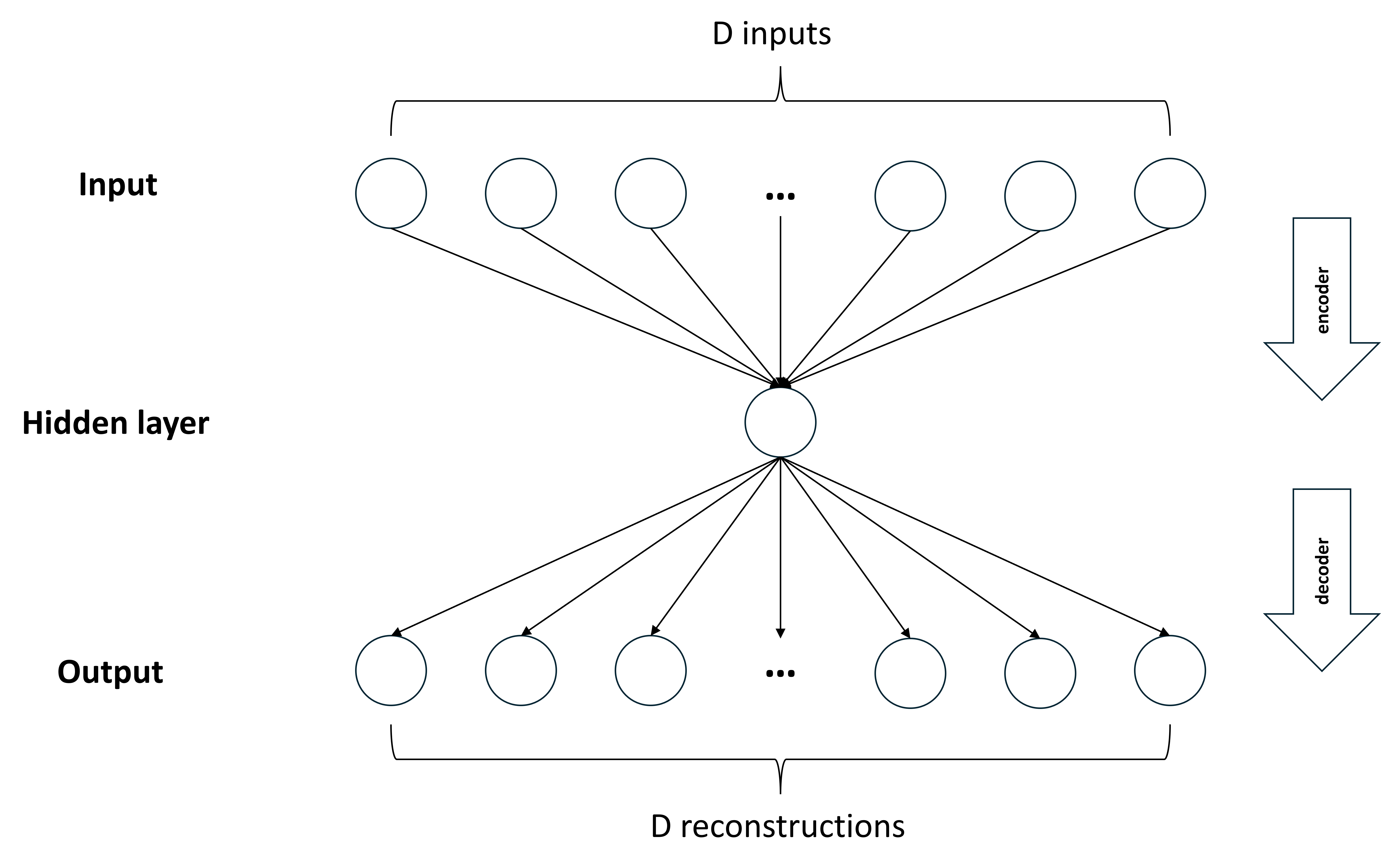
The autoencoder is a special neural network model designed to generate the output that approximates the input data. This autoencoder is composed of two main components: an encoder and a decoder (Gu et al.,, 2021). The inputs are transformed through a relatively smaller number of neurons in the hidden layer(s) than the dimension of inputs, resulting in a low-dimensional encoded representation of the inputs. This process is called encoding and happens in the “encoder”. The encoded data are then transformed through a “decoder” network with an opposite structure of “encoder”, to recover the encoded data, resulting in a reconstruction of inputs. The whole system is called an “autoencoder”. Since the autoencoder generates output to approximate its input, no labelled data is needed. The autoencoder is trained as an unsupervised process. However, the training process is still based on the optimisation of minimising the discrepancy between the input data and its reconstruction in the output (Hinton and Salakhutdinov,, 2006).
Autoencoder with L hidden layers can be written as the recursive formula. Denote as the number of neurons in layer , where . The input and output of a single neuron in layer can be written as:
where is the input sent to neuron , is the output. is the weight that connects neuron in layer to neuron in layer , is the bias for neuron . The input is transformed through an activation function , becoming the output and being passed to the next layer. Define the vector of all inputs to layer as , and outputs of this layer as . The output in layer can then be written in a matrix notation as
| (13) |
where , is a matrix of weight parameters, and is a bias vector. The final output at layer of the autoencoder is:
| (14) |
where the final output has the same dimension as the input.
Ideally, an autoencoder could employ multiple hidden layers and neurons, allowing for deep learning and more nuanced feature extraction. However, increasing network complexity can make training significantly harder. Without proper pretraining, a deep autoencoder often fails to capture patterns effectively, instead outputting a result that approximates the average of the input data. As Hinton and Salakhutdinov, (2006) note, this issue can persist despite extensive fine-tuning, whereas a shallower autoencoder with a single hidden layer can learn without the need for pretraining. Given the complexity and time-consuming nature of the deep autoencoder, this thesis employs a single hidden-layer autoencoder as a starting point to explore the effectiveness of nonlinear dimension reduction, with plans to extend to a deeper architecture in future work.
In this design, the layer between the input and the hidden layer works as an encoder, transforming the input to the hidden representation. The layer between the hidden layer and the output works as a decoder, reconstructing the original input. To initialise, the input is the realised volatility measures vector , , as defined in Equation (5). Thus, with . There is one neuron in the hidden layer , as its output is used to incorporate into univariate RealGARCH. We use the sigmoid function as nonlinear activation functions in two layers, . Let denote the initial input , denote the output of the encoder layer , and denote the output of the decoder layer . The autoencoder in this thesis can be written as:
| (15) | ||||
where is a encoded value (scalar) at time , is a vector of weight parameters for the encoder, and is a scalar of bias parameter. is a vector of weight parameters for the decoder, and is a vector of bias parameters. and . Over period , the autoencoder generates a synthetic realised measure vector , composed of scalar outputs for each time . Like , and , serves as the synthetic realised measure series. But is obtained through nonlinear dimension reduction of realised measures, different to the linear dimension reduction in PCA, ICA and average. Figure 1 illustrates the architecture of the autoencoder employed in this thesis, where the input and output are displayed in a horizontal layout for visualisation purpose.
Empirically, the weights and biases of the autoencoder can be estimated by minimising the loss function between input and its reconstruction , we adopt Mean Squared Error (MSE) here:
| (16) |
where represents the th feature of the input realised measures input at time , while represents the corresponding reconstructed feature at time .
3.2.2 Regularised Autoencoder
The Autoencoder shares a similar essence with neural networks. The high capacity of neural networks gives the autoencoder more flexibility in extracting significant features from the data. However, this highly flexible characteristic is directly related to the complexity of the model. The standard autoencoder is trained based on minimising the loss function in Equation (16), which typically leads to the underlying overfitting problem. Motivated by Gu et al., (2021), we considered the use of regularisation to prevent overfitting in two aspects: weights and sparsity.
Weight Regularisation
The most common type of regularisation is to add a complexity penalty to the optimisation objective. We define the optimisation objective as:
| (17) |
where is a hyperparameter and is the regulariser that measures the complexity of the model as a function of weight parameters.
There are many choices for penalty functions, such as Ridge and Lasso. Given that the input data consists of realised volatility measures, which are different approaches to measuring realised volatility, these features are closely relevant to each other. Compared to Lasso, which assigns substantial coefficients to a small number of features, Ridge is more suitable in this context, as it assigns similar and small coefficients to all features, better capturing the correlated relationships among measures. Therefore, we use Ridge regularisation which takes the form:
| (18) |
where is the weight connecting input and the neuron in the first layer, is the weight connecting the neuron and output in the second layer. The Ridge regularisation term is the sum of squared elements of the weight vectors for each layer.
Sparsity Regularisation
In addition to weight regularisation, sparsity regularisation also encourages the autoencoder to find a more general and robust representation of the input data by constraining the activation value. This helps prevent the autoencoder from fitting to noise and learning undesired variations, ensuring that the encoded data captures consistent patterns in realised measures instead of noise. This regularisation works on the average output activation value of the neuron in the hidden layer, the average of this neuron from the training samples with a size of can be expressed as:
| (19) |
The sparsity regularisation aims to restrict the value of to be low, preventing the encoded data from fluctuating significantly when the original data do not show extreme variations.
The sparsity regularisation is designed to give a large penalty when the average activation value is not close to the settled value . We use the Kullback-Leibler divergence as the function, which has the form:
| (20) |
where KL provides a value of 0 only when and are equal to each other, but provides a large value when they diverge from each other. Therefore, minimising this sparsity regularisation term enforces approaching as close as possible.
Finally, the parameters in the autoencoder , , and for a dataset with size can be estimated by minimising the overall loss function , which is designed as:
| (21) |
where and control the magnitude of the penalty in the loss function, and controls the desired value of the average activation value.
3.2.3 Autoencoder Enhanced Realised GARCH
The autoencoder-produced realised measure series , consisting of , can be obtained by first estimating parameters through minimising the loss function in Equation (21), and then applying these estimated parameters to the autoencoder formula in Equation (15). Similarly to realised measure series , and , includes a linear weighted combination process but also has an additional nonlinear transformation process using the sigmoid activation function. Additionally, in terms of decomposition purposes, PCA and ICA are designed to produce uncorrelated and independent components, respectively. However, the autoencoder encoded the realised measures into a synthetic measure which can be decoded back to the original realised measures with minimum accuracy loss. Here, we denote , , and in row vector formats as shorthands for their transposed forms for later reference.
The nonlinear dimensionality-reduced realised measure is then rescaled by Equation (7), to fall within the typical range of realised measures. Replace the single realised measure in RealGARCH, we propose an autoencoder enhanced RealGARCH (AE-RealGARCH):
| (22) | ||||
In the empirical study section, we will compare the volatility forecasting performance of AE-RealGARCH, PC-RealGARCH, IC-RealGARCH and AVG-RealGARCH to evaluate the improvements offered by the autoencoder-produced synthetic measure.
3.3 Model Estimation
The AE-RealGARCH, PC-RealGARCH, IC-RealGARCH and AVG-RealGARCH models employ different processes on realised measure , but their underlying volatility modelling principles are all rooted in the RealGARCH framework. The estimation of these models adheres to the procedures established for RealGARCH, as outlined by Hansen et al., (2012), where parameters as estimated by maximising the likelihood function. Accordingly, the following section presents the likelihood function for RealGARCH as a representative example.
Given the return and realised volatility measure can be observed at day , the Maximum Likelihood (ML) can be used here to find the parameters in RealGARCH that make these two observed data most probable under our specified model. Following the approach of Hansen et al., (2012), the joint likelihood in RealGARCH is equal to the sum of two likelihood functions.
Let denote here for consistent presentation, we assume Gaussian distributions , and . Therefore the zero-mean returns are given by and the “de-meaned” realised measure is modelled as: . The distributions can be expressed as: , . In this case, the probability density function (PDF) of and are:
| (23) | ||||
The joint log-likelihood function for RealGARCH, omitting constant terms, can then be written as the sum of two log-likelihood functions for returns and realised measure :
| (24) |
where , . In AE-RealGARCH, replace with ; in PC-RealGARCH, replace with ; and similarly, use and for IC-RealGARCH and AVG-RealGARCH, respectively. is the training sample size. summarise the parameters . and represent the log-likelihood functions for returns component and realised measure component, respectively. Consequently, the parameters in the RealGARCH model can be estimated by maximising the log-likelihood function , while considering the constraint in Equation (4).
It is worth noting that, GARCH-type models such as GARCH and GARCH-X do not have the log-likelihood function for realised measure , their parameters are estimated based on the maximisation of only. In this case, differences in the log-likelihood function specifications between RealGARCH and GARCH-type models make the direct comparison of the overall maximised log-likelihood challenging. In this case, the common log-likelihood term for returns , allows for a meaningful comparison for assessment purpose (Naimoli et al.,, 2022).
Since the optimisation objective includes an inequality constraint as in Equation (4), Sequential Least Squares Programming (SLSQP) is used to solve the constrained optimisation problem. Developed by Kraft, (1988), SLSQP is implemented as an optimisation method in Python’s Scipy library. Compared to standard gradient descent, SLSQP does not require specifying the learning rate and batch size at the beginning. Known for reaching global convergence and superlinear convergence speed (Xie et al.,, 2020), SLSQP ensures the resulting parameters satisfy the constraint condition in Equation (4).
All GARCH-type models are estimated using the Python code developed for this thesis. The synthetic realised measures from PCA and ICA, , , are computed using Scikit-learn library in Python, while is obtained with Matlab’s Deep Learning Toolbox.
4 Empirical Study
4.1 Data Description
Four daily international stock market indices are analysed in this study: the S&P 500 (US); FTSE 100 (UK); AORD (Australia); Hang Seng (Hong Kong). Data for the daily closing price index from January 2000 to June 2022 are collected from The Oxford-Man Institute’s Realised Library. These closing prices are used to calculate daily returns. The daily percentage log returns are calculated as , where is the closing price on day . The returns are then de-meaned. Since the return requires the closing price on the previous day, the first row of each market data is removed to match the series of returns. The market-specific non-trading days are removed from each market data. After these adjustments, the whole dataset sizes for four markets are approximately 5600 days, with the largest size being 5668 days in AORD and the smallest size being 5504 days in Hang Seng.
In addition, 12 realised volatility measures introduced in Section 2.1.2, are included in the dataset: Realised Variance (RV) (Andersen and Bollerslev,, 1998), Realised Semivariance (RSV) (Barndorff-Nielsen et al., 2008c, ), Median Realised Variance (MedRV) (Andersen et al.,, 2012), Realised Kernel (RK) (Barndorff-Nielsen and Shephard,, 2002), Two-scale Realised Kernel (TwoScale RK) (Ikeda,, 2015), Parzen Weighted Realised Kernel (Parzen RK) (Barndorff-Nielsen et al., 2008b, ), Bipower Variation (BV) (Barndorff-Nielsen,, 2004), computed at 5 and 10-minute frequencies and combined with subsampling technique (Zhang et al.,, 2005), resulting 12 different realised measures. These 12 realised measures are calculated based on the high-frequency data within the trading time, and they are used as the input to generate the synthetic realised measure using PCA, ICA, average, and autoencoder, respectively. Hence, the input dimension in Equation (5) is 12 in this thesis.
| Mean | Std.Dev | Median | Min | Max | Skewness | Kurtosis | |
|---|---|---|---|---|---|---|---|
| 0.000 | 1.242 | 0.044 | -12.687 | 10.625 | -0.393 | 10.120 | |
| -0.679 | 1.146 | -0.744 | -4.408 | 4.350 | 0.356 | 0.339 | |
| -0.691 | 1.172 | -0.747 | -4.344 | 4.355 | 0.329 | 0.303 | |
| -1.480 | 1.246 | -1.543 | -6.101 | 3.563 | 0.302 | 0.202 | |
| -1.594 | 1.224 | -1.676 | -6.753 | 3.363 | 0.350 | 0.268 | |
| -0.679 | 1.146 | -0.744 | -4.408 | 4.350 | 0.356 | 0.339 | |
| -0.691 | 1.172 | -0.747 | -4.344 | 4.355 | 0.329 | 0.303 | |
| -1.480 | 1.246 | -1.543 | -6.101 | 3.563 | 0.302 | 0.202 | |
| -0.795 | 1.108 | -0.870 | -4.135 | 4.422 | 0.412 | 0.390 | |
| -0.798 | 1.220 | -0.839 | -4.711 | 3.933 | 0.266 | 0.207 | |
| -0.786 | 1.115 | -0.861 | -4.113 | 4.444 | 0.406 | 0.347 | |
| -0.876 | 1.138 | -0.951 | -4.551 | 4.097 | 0.414 | 0.384 | |
| -0.876 | 1.138 | -0.951 | -4.551 | 4.097 | 0.414 | 0.384 |
Table 1 reports the summary statistics of daily percentage log returns and 12 log-transformed daily realised volatility measures in the S&P 500. Similar patterns are observed in the other three markets, where the daily percentage log returns following a de-mean process have a mean value of 0, exhibiting positive excess kurtosis, persistent heteroskedasticity, and negative skewness. The original realised volatility measures are all positive and obvious right-skewed distributions, the log-transformed realised measures display the properties of mitigated positive skewness and positive excess kurtosis. Furthermore, the statistics for the realised measures closely align with those of the sub-sampled realised measures.
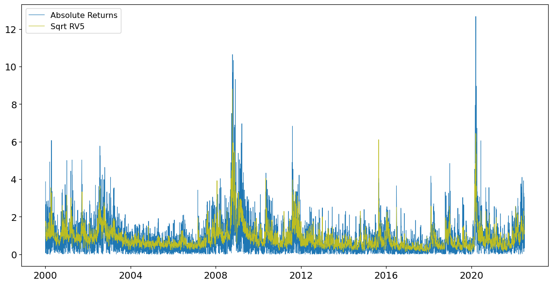
Figure 2 displays the plot of absolute log percentage returns and the square root of 5-min RV for the full dataset of S&P 500. The consistent pattern between these two series indicates the effectiveness of the realised volatility measure as a proxy for the underlying volatility influencing returns. Notably, the high volatility periods are associated with significant fluctuation events. The burst of the tech bubble caused market volatility from 2000 to 2002, while the GFC of 2007-2008, triggered by the collapse of the US housing market, resulted in significant volatility during that period. Additionally, the crisis that spread from the banking system to sovereign debt issues in Europe was evident in late 2011. Finally, the immediate global impact of COVID-19 led to an unprecedented surge in market volatility during 2019-2020.
The full dataset is divided into two disjoint time periods, comprising approximately 80% and 20% of the data while maintaining the temporal order. The first subsample, in-sample, from January 2000 to December 2017, including the period of the GFC, is used to estimate the models. The second subsample, out-of-sample, from January 2018 to June 2022, including the period of COVID-19, is used for comparing the predictive performance of models. There are some small differences in the size of in-sample and out-of-sample across markets due to the specific non-trading days in each market. The resulting in-sample sizes for all four markets are approximately 4500 days, with the largest size being 4537 days in AORD and the smallest being 4412 days in Hang Seng. The out-of-sample sizes for four markets are around 1100 days, with the largest size being 1133 days in AORD and the smallest size being 1092 days in Hang Seng.
4.2 In-sample Analysis
4.2.1 In-sample Series
This section illustrates the synthetic realised measures derived from PCA, ICA, average and autoencoder approaches for in-sample data of all markets. As the data split described in Section 4.1, the in-sample size for S&P 500 is 4517 days, and estimated model parameters for the S&P 500 are displayed here for discussion.
Table 2 shows the statistical summary of synthetic measures after log transformation. Since these synthetic measures undergo log transformation when incorporated into the RealGARCH model, the table provides their log-transformed statistics, facilitating comparison with Table 1. Specifically, , and share the same minimum and maximum values, because they all have been rescaled according to Equation (7) to fit within the minimum and maximum values of realised measures, shown in Table 1. Moreover, the highly close statistics of and indicate a strong similarity between the two series, suggesting that both PCA and ICA capture similar patterns in decomposition.
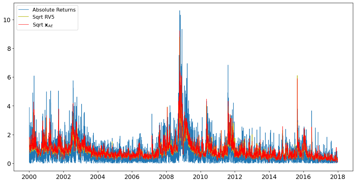
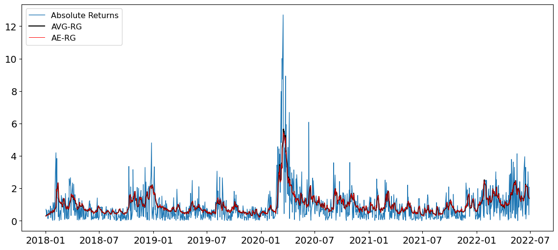
Figure 3 shows that the synthetic realised measure generated from the autoencoder has a similar pattern to that of the realised volatility measure, such as 5-min RV, effectively capturing the changing pattern in absolute returns. This means that the autoencoder can successfully generate a synthetic realised measure through nonlinear dimension reduction from multiple realised measures, to serve as a proxy for the underlying volatility.
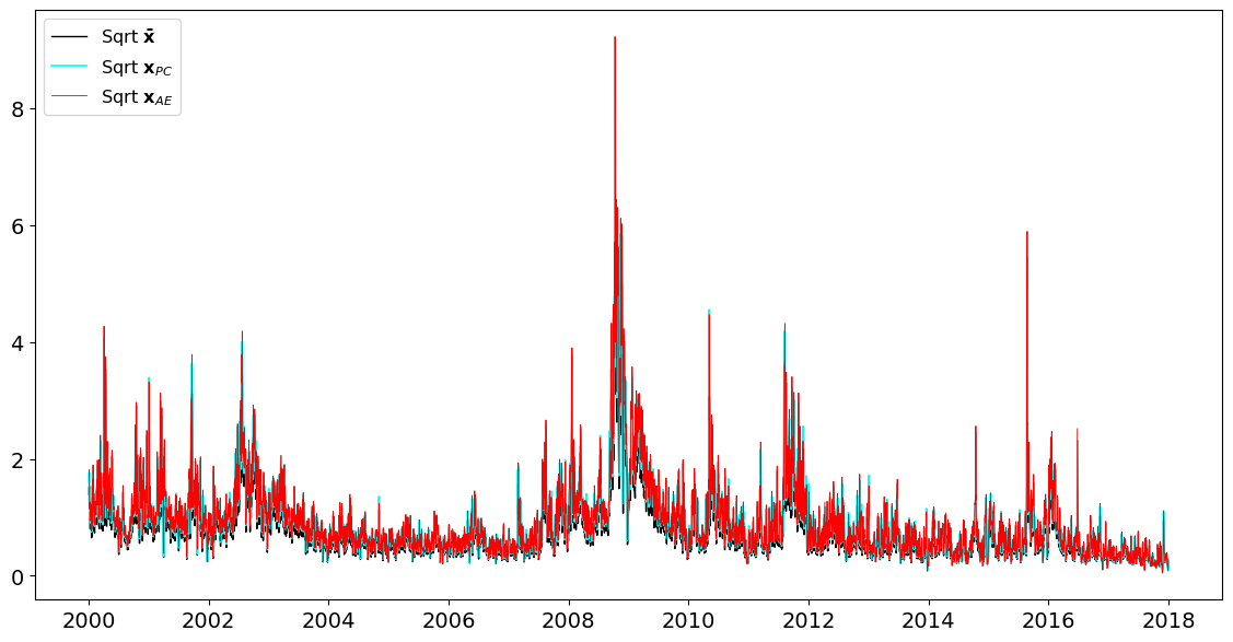
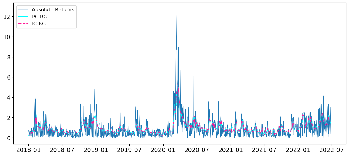
Figure 4 displays that the nonlinear combined realised measure from autoencoder shares a similar pattern to those of linear-combined measures, such as PCA and average. Given and are highly close as shown in Table 2, only the realised measure from PCA, , is displayed here to maintain visual clarity. This similarity suggests that the autoencoder captures core dynamic volatility, which is comparable to traditional linear combined methods. This novel representation of volatility offers an opportunity to improve the predictive performance and robustness of volatility modelling.
| Mean | Std.Dev | Median | Min | Max | Skewness | Kurtosis | |
|---|---|---|---|---|---|---|---|
| S&P500 | |||||||
| -0.532 | 1.179 | -0.572 | -6.101 | 4.444 | 0.202 | 0.479 | |
| -0.582 | 1.171 | -0.617 | -6.101 | 4.444 | 0.195 | 0.496 | |
| -0.582 | 1.171 | -0.617 | -6.101 | 4.444 | 0.195 | 0.496 | |
| -0.845 | 1.129 | -0.903 | -4.524 | 4.135 | 0.340 | 0.359 | |
| FTSE | |||||||
| 0.019 | 1.074 | -0.039 | -7.062 | 4.838 | 0.300 | 0.781 | |
| -0.396 | 1.087 | -0.465 | -7.062 | 4.838 | 0.309 | 0.689 | |
| -0.396 | 1.087 | -0.465 | -7.062 | 4.838 | 0.309 | 0.689 | |
| -0.654 | 1.005 | -0.747 | -3.512 | 4.477 | 0.569 | 0.520 | |
| AORD | |||||||
| -0.651 | 0.968 | -0.728 | -6.063 | 3.344 | 0.389 | 0.701 | |
| -0.864 | 1.023 | -0.943 | -6.063 | 3.344 | 0.377 | 0.635 | |
| -0.864 | 1.023 | -0.943 | -6.063 | 3.344 | 0.377 | 0.635 | |
| -1.409 | 0.957 | -1.505 | -4.657 | 2.643 | 0.542 | 0.564 | |
| Hang Seng | |||||||
| -0.187 | 0.957 | -0.251 | -6.034 | 4.219 | 0.330 | 0.859 | |
| -0.205 | 0.949 | -0.275 | -6.034 | 4.219 | 0.365 | 0.880 | |
| -0.205 | 0.949 | -0.275 | -6.034 | 4.219 | 0.365 | 0.880 | |
| -0.662 | 0.856 | -0.757 | -3.126 | 3.634 | 0.676 | 0.780 |
4.2.2 In-sample Parameters
The estimated parameters of two GARCH-type models and five RealGARCH-type models are presented in Table 3. Overall, the GARCH equation parameters are comparable among these models, and the consistency of measurement equation parameters can be observed.
In terms of the GARCH equation, in standard GARCH and GARCH-X is the coefficient of lagged squared returns and realised measure, respectively. Since GARCH-X replaces the squared returns with the more informative realised measure, specifically 5-min RV here, the value of is much higher than in standard GARCH. This higher indicates that GARCH-X assigns more weight to the realised measure than squared returns, enhancing its contribution to volatility modelling. Therefore, GARCH-X has a lower training negative log-likelihood value than standard GARCH, indicating the improvement when using the more efficient realised measure during the training process. In RealGARCH models, is the coefficient for the lagged realised measure term, comparable to the in GARCH and GARCH-X models. The values of in PC-RealGARCH, IC-RealGARCH, AVG-RealGARCH, and AE-RealGARCH are around 0.36 to 0.38, illustrating the comparable effectiveness of synthetic realised measures.
In terms of the measurement equation, there are 5 parameters in RealGARCH models specifically. The values for these 5 parameters are consistent with the estimates in Table : “Results for the log-linear specification” of Hansen et al., (2012). The estimates of in RealGARCH models are all close to unity, suggesting that the synthetic realised measure is roughly proportional to the conditional variance of daily returns. The always negative estimates of reflect that a negative bias correction is needed in the regression of realised measure and the conditional variance of returns. One potential explanation for this is that the returns calculated in this thesis are based on close-to-close prices, including the overnight period (e.g. 24 hours) for prices to fluctuate. In contrast, the synthetic realised measure is derived from various realised measures, which are captured during the opening hours of the market (e.g., 6.5 hours). This shorter calculation period may lead to an underestimation of the underlying volatility of returns on average. Therefore, should be expected, and a downside bias correction is required to align the conditional variance of returns with realised measures, resulting in the log-transformed realised measure being a biased estimator of the true log-transformed volatility.
Regarding the leverage effect term , the estimates of are all below 0, which is consistent with the famous phenomenon in stock markets of negative correlation between today’s return and tomorrow’s volatility (Nelson,, 1991). To be specific, given , is negative when the return , then is a positive value. Combining this positive value with produces a larger term, resulting in a larger in the measurement equation than that of . Then this larger will lead to a larger volatility when predicting through the GARCH equation as the coefficient of is positive. Consequently, these estimates of parameters successfully reflect the existing leverage effect in markets.
| GARCH | GARCH-X | RV-RG | PC-RG | IC-RG | AVG-RG | AE-RG | |
|---|---|---|---|---|---|---|---|
| 0.0148 | 0.0387 | 0.1536 | 0.1334 | 0.1334 | 0.2417 | 0.1155 | |
| 0.8932 | 0.6816 | 0.5982 | 0.5743 | 0.5743 | 0.5707 | 0.5718 | |
| 0.0949 | 0.3184 | 0.3566 | 0.3669 | 0.3669 | 0.3840 | 0.3712 | |
| -0.4475 | -0.3803 | -0.3803 | -0.6457 | -0.3281 | |||
| 1.0487 | 1.0828 | 1.0828 | 1.0443 | 1.0760 | |||
| -0.1010 | -0.1332 | -0.1332 | -0.1447 | -0.1823 | |||
| 0.1165 | 0.1136 | 0.1136 | 0.1062 | 0.1072 | |||
| 0.5374 | 0.5324 | 0.5324 | 0.5025 | 0.5288 | |||
| 4019.5764 | 3708.9311 | 3681.8538 | 3687.5621 | 3687.5621 | 3665.8649 | 3670.8105 |
4.3 Out-of-sample Forecasting
4.3.1 Forecasting Performance
For each market, the out-of-sample period spans approximately 1090 to 1130 days, starting on 2 January 2018 and ending on 28 June 2022. The parameters mentioned above, generated from the first estimation window (in-sample, 4 January 2000 to 31 December 2017), are used to produce the first one-step-ahead forecast for 2 January 2018 in out-of-sample. Then, the estimation window is slid forward by one day, maintaining a fixed window size. The synthetic realised measure series , , and are re-generated based on the updated estimation window to re-estimate each model and produce the forecast for the next day. This rolling process is repeated daily until forecasts are generated for all days in the out-of-sample period across all models. Eventually, we obtained a total of approximately 1090 to 1130 one-step-ahead forecasts for each market.
Specifically, the hyperparameter values for , and in Equation (21) are set to 0.001, 0.001, and 0.05, respectively, which correspond to the default values of hyperparameters in “trainAutoencoder” function in Matlab. To pursue a more accurate encoding effect, the hyperparameters should ideally be selected through the validation process within each rolling window. However, due to the computational cost, we use the default values in this case, which work well in the empirical study with comprehensive tests. The encoded series has a desired pattern with realised measures in each rolling window, as shown in Figure 3. It is noted that in some rolling window forecasting steps, the autoencoder may generate encoded series with unintended patterns by estimating negative weights in the encoder. This is because the negative weights can cause the input values to approach negative infinity more readily than positive weights would, thereby resulting in the average activation value that is more easily closer to the desired level through the sigmoid activation function . In this case, we re-run those steps, which then yield series with desired patterns.
As introduced in Section 3.3, the common log-likelihood function part is used to compare between models. To assess the volatility forecasting performance, can be used to calculate the predictive log-likelihood values. According to Gerlach and Wang, (2016), the predictive log-likelihood function can be written as:
where starts from the first day in out-of-sample. For the first predictive log-likelihood value, is the forecasted variance based on estimated parameters () and all available information up to and including time . is the squared return observed at time . Generally, the forecast volatility is generated at time ; when time advances to , the observed return allows to be used as a measure of predictive accuracy. These calculations are performed for each day in the out-of-sample period and eventually summed to estimate the overall predictive log-likelihood for each model.
Table 4 reports the predictive log-likelihood values for GARCH, GARCH-X and RealGARCH using 5-min RV, PC-RealGARCH, IC-RealGARCH, AVG-RealGARCH, and AE-RealGARCH in four markets.
First, in all markets, GARCH-X replacing squared returns with realised volatility measure, 5-min RV, consistently shows a lower negative predictive log-likelihood compared to standard GARCH using squared returns. This aligns with the findings of Engle, (2002). The in-sample parameters analysis in Section 4.2.2 may partially explain this improvement. Additionally, RealGARCH extends GARCH-X by adding a measurement equation, while still using the same 5-min RV, further improving the predictive accuracy in three out of four markets.
| S&P 500 | FTSE | AORD | Hang Seng | |
| GARCH | 1168.0 | 1119.9 | 736.1 | 1666.9 |
| GARCH-X | 1074.3 | 1044.0 | 731.5 | 1637.8 |
| RV-RG | 1011.4 | 1046.3 | 727.0 | 1625.2 |
| PC-RG | 1000.5 | 1047.4 | 722.4 | 1626.3 |
| IC-RG | 1000.5 | 1047.4 | 722.4 | 1626.3 |
| AVG-RG | 992.8 | 1040.9 | 719.5 | 1624.7 |
| AE-RG | 990.9 | 1036.0 | 719.8 | 1627.3 |
| 4517 | 4533 | 4535 | 4412 | |
| 1117 | 1129 | 1133 | 1092 |
Second, PC-RealGARCH and IC-RealGARCH, which use the synthetic realised measure and derived from PCA and ICA, respectively, exhibit the same predictive log-likelihood values across all markets. This similarity could be explained by the similarity of log-transformed series, and , in Section 4.2.1, as well as the estimated parameters incorporated into PC-RealGARCH and IC-RealGARCH, as described in Section 4.2.2. The statistical summaries of and , along with the parameter estimates and training negative log-likelihood values, are highly similar in PC-RealGARCH and IC-RealGARCH. Therefore, the high similarity between the two models suggests that, although PCA and ICA are based on different principles, targeting uncorrelation and independence, respectively, their decompositions of realised measures produce highly coincident results. This illustrates that PCA and ICA may not provide significantly different benefits when dealing with realised volatility measures.
Finally, the proposed model AE-RealGARCH ranks first in volatility forecasting for S&P 500 and FTSE, and second for AORD, demonstrating its solid performance among the competing models. The other fairly competitive model is the AVG-RealGARCH, which consistently ranks first or second for all markets, outperforming linear dimension reduction techniques like PCA and ICA. This observation motivates the exploration of nonlinear dimension reduction techniques for realised measures. In this regard, generated through a nonlinear transformation in autoencoder, gaining additional flexibility and capturing more information about volatility, provides a more effective and informative realised volatility measure than linear methods, resulting in a reliable AE-RealGARCH.
Figure 5 shows the forecasted volatility series of AE-RealGARCH, AVG-RealGARCH, PC-RealGARCH and IC-RealGARCH, respectively. All models exhibit forecasted volatility series that consistently align with the absolute returns in the out-of-sample period, indicating that RealGARCH models using synthetic realised measures effectively capture and forecast dynamic volatility. Specifically, the forecasted volatility series in PC-RealGARCH and IC-RealGARCH are nearly identical, meaning that RealGARCH using whether or produces highly close forecasted volatility results, which is in line with the predictive log-likelihood analysis discussed above.
4.3.2 Out-of-sample Parameters
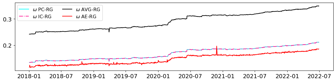
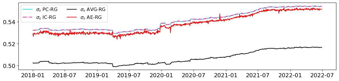
To further illustrate the impact of linear and nonlinear dimension reduction techniques on the synthetic realised measure within the RealGARCH model, Figure 6 presents parameter estimates of , , in the GARCH equation, as well as in measurement equation, across each forecasting step for S&P 500 out-of-sample period. Results are shown for the PC-RealGARCH, IC-RealGARCH, AE-RealGARCH and AVG-RealGARCH models, respectively.
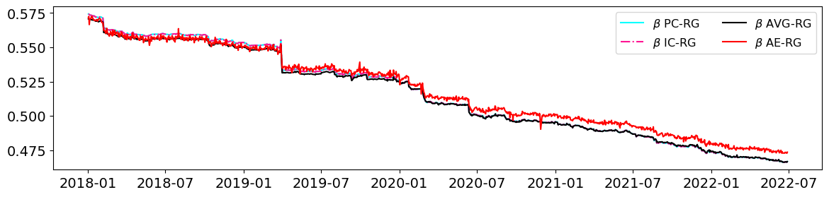
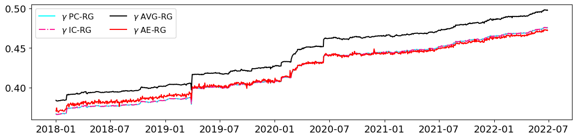
First, regarding the parameters in the GARCH equation, the estimated value of continuously increases over time, while the estimate of decreases correspondingly. This indicates that as RealGARCH forecasts volatility, it gradually relies on the realised measure during the out-of-sample period. The realised measure contributes progressively more to the model. Additionally, the estimates of parameters , and in the AE-RealGARCH exhibit significantly larger fluctuations than those of other models. One potential reason for this is that AE-RealGARCH incorporates the realised measure produced by autoencoder , keeping a high sensitivity to each day’s volatility. As a result, AE-RealGARCH has more flexibility to adjust the parameters in each forecasting step, effectively capturing the time-varying nature of volatility. The parameter estimates in PC-RealGARCH and IC-RealGARCH are almost identical in each rolling forecast window, which can further confirm the similar effect of PCA and ICA on realised measures discussed in Section 4.3.1.
Second, regarding the measurement equation, the frequently fluctuated volatility in AE-RealGARCH indicates the synthetic realised measure has a more fluctuating volatility in each rolling window. Compared with , and which are obtained by linearly combining series with weights, is derived from a linear combination with weights first, followed by a nonlinear activation function , specifically the sigmoid function in this thesis. This nonlinear activation function provides additional flexibility, enabling it to effectively capture the underlying volatility across numerous realised measures, thus resulting in greater adaptability in each rolling window.
5 Conclusion and Future Research
5.1 Conclusion
In this thesis, we propose an autoencoder enhanced RealGARCH that relies on a synthetic realised volatility measure obtained through the nonlinear dimension reduction of the autoencoder. This choice led to significant improvements in the out-of-sample predictive performance, compared to RealGARCH employing a single realised measure; linearly dimension-reduced synthetic realised measure from PCA, ICA and average, respectively, as well as traditional GARCH models. Furthermore, this study provides a new perspective for volatility modelling when researchers face the challenge of selecting a single volatility measure from multiple candidates. Instead of subjective selection, AE-RealGARCH synthesises the information from different realised measures into a robust component for model fitting and forecasting. The intended flexibility of the nonlinear transformation is evident through the more flexible parameter estimates in each rolling window, highlighting the ability of the autoencoder to capture complex patterns beyond the limitations of linear methods. This adaptability confirms the advantage of using nonlinear synthesis for volatility forecasting.
5.2 Limitations and Extensions
This study could be extended in the following ways. First, the autoencoder designed in this thesis has a single hidden layer for dimension reduction, and the input realised measures are directly transformed into a one-dimensional measure for RealGARCH. It is worthwhile to extend the single hidden layer autoencoder into a multilayer format, as in Hinton and Salakhutdinov, (2006). Additionally, incorporating uncertainty measures based on financial news, such as economic policy uncertainty (Baker et al.,, 2016), alongside realised volatility measures could enrich the model’s input. This approach could allow the dimension-reduced output to be more than one dimension, thereby enhancing its integration with the RealEGARCH model. Second, the hyperparameter values for the autoencoder are set to the default values in Matlab, and the same hyperparameters are used for the subsequent rolling window steps to minimise computational cost. Further improvement involves validation setting for more advanced hyperparameter selection in each rolling window step, to tune based on different volatility conditions on each day. Lastly, this study employs Gaussian distribution for errors in returns to estimate models. Future research could consider more appropriate distributions, such as Student- errors, to further enhance forecasting accuracy.
References
- Alexander, (2001) Alexander, C. (2001). Market Models: A Guide to Financial Data Analysis. University of Sussex.
- Andersen and Bollerslev, (1998) Andersen, T. G. and Bollerslev, T. (1998). Answering the Skeptics: Yes, Standard Volatility Models do Provide Accurate Forecasts. International Economic Review, 39(4):885–905.
- Andersen et al., (2003) Andersen, T. G., Bollerslev, T., Diebold, F. X., and Labys, P. (2003). Modeling and Forecasting Realized Volatility. Econometrica, 71(2):579–625.
- Andersen et al., (2012) Andersen, T. G., Dobrev, D., and Schaumburg, E. (2012). Jump-robust volatility estimation using nearest neighbor truncation. Journal of Econometrics, 169(1):75–93.
- Andersen and Teräsvirta, (2009) Andersen, T. G. and Teräsvirta, T. (2009). Realized Volatility. In Mikosch, T., Kreiß, J.-P., Davis, R. A., and Andersen, T. G., editors, Handbook of Financial Time Series, pages 555–575. Springer, Berlin, Heidelberg.
- Baker et al., (2016) Baker, S. R., Bloom, N., and Davis, S. J. (2016). Measuring Economic Policy Uncertainty*. The Quarterly Journal of Economics, 131(4):1593–1636.
- Baldi, (2012) Baldi, P. (2012). Autoencoders, Unsupervised Learning, and Deep Architectures. In Proceedings of ICML Workshop on Unsupervised and Transfer Learning, pages 37–49. JMLR Workshop and Conference Proceedings.
- Bao et al., (2017) Bao, W., Yue, J., and Rao, Y. (2017). A deep learning framework for financial time series using stacked autoencoders and long-short term memory. PLOS ONE, 12(7):e0180944.
- Barndorff-Nielsen, (2004) Barndorff-Nielsen, O. E. (2004). Power and Bipower Variation with Stochastic Volatility and Jumps. Journal of Financial Econometrics, 2(1):1–37.
- (10) Barndorff-Nielsen, O. E., Hansen, P. R., Lunde, A., and Shephard, N. (2008a). Designing Realised Kernels to Measure the Ex-Post Variation of Equity Prices in the Presence of Noise. SSRN Electronic Journal.
- (11) Barndorff-Nielsen, O. E., Hansen, P. R., Lunde, A., and Shephard, N. (2008b). Realised Kernels in Practice: Trades and Quotes. SSRN Electronic Journal.
- (12) Barndorff-Nielsen, O. E., Kinnebrock, S., and Shephard, N. (2008c). Measuring Downside Risk - Realised Semivariance. SSRN Electronic Journal.
- Barndorff-Nielsen and Shephard, (2002) Barndorff-Nielsen, O. E. and Shephard, N. (2002). Econometric Analysis of Realized Volatility and its Use in Estimating Stochastic Volatility Models. Journal of the Royal Statistical Society Series B: Statistical Methodology, 64(2):253–280.
- Bollerslev, (1986) Bollerslev, T. (1986). Generalized autoregressive conditional heteroskedasticity. Journal of Econometrics, 31(3):307–327.
- Cao et al., (2003) Cao, L., Chua, K., Chong, W., Lee, H., and Gu, Q. (2003). A comparison of PCA, KPCA and ICA for dimensionality reduction in support vector machine. Neurocomputing, 55(1-2):321–336.
- Chen et al., (2007) Chen, Y., Härdle, W., and Spokoiny, V. (2007). Portfolio value at risk based on independent component analysis. Journal of Computational and Applied Mathematics, 205(1):594–607.
- Christensen and Podolskij, (2007) Christensen, K. and Podolskij, M. (2007). Realized range-based estimation of integrated variance. Journal of Econometrics, 141(2):323–349.
- Christensen et al., (2017) Christensen, K., Podolskij, M., Thamrongrat, N., and Veliyev, B. (2017). Inference from high-frequency data: A subsampling approach. Journal of Econometrics, 197(2):245–272.
- Cortés et al., (2024) Cortés, D. G., Onieva, E., López, I. P., Trinchera, L., and Wu, J. (2024). Autoencoder-Enhanced Clustering: A Dimensionality Reduction Approach to Financial Time Series. IEEE Access, 12:16999–17009.
- Engle, (2002) Engle, R. (2002). New frontiers for arch models. Journal of Applied Econometrics, 17(5):425–446.
- Engle, (2004) Engle, R. (2004). Risk and Volatility: Econometric Models and Financial Practice. American Economic Review, 94(3):405–420.
- Engle, (1982) Engle, R. F. (1982). Autoregressive Conditional Heteroscedasticity with Estimates of the Variance of United Kingdom Inflation. Econometrica, 50(4):987–1007.
- Fan et al., (2008) Fan, J., Wang, M., and Yao, Q. (2008). Modelling Multivariate Volatilities via Conditionally Uncorrelated Components. Journal of the Royal Statistical Society Series B: Statistical Methodology, 70(4):679–702.
- García-Ferrer et al., (2012) García-Ferrer, A., González-Prieto, E., and Peña, D. (2012). A conditionally heteroskedastic independent factor model with an application to financial stock returns. International Journal of Forecasting, 28(1):70–93.
- Gerlach and Wang, (2016) Gerlach, R. and Wang, C. (2016). Forecasting risk via realized GARCH, incorporating the realized range. Quantitative Finance, 16(4):501–511.
- Gu et al., (2021) Gu, S., Kelly, B., and Xiu, D. (2021). Autoencoder asset pricing models. Journal of Econometrics, 222(1):429–450.
- Hansen and Huang, (2016) Hansen, P. R. and Huang, Z. (2016). Exponential GARCH Modeling With Realized Measures of Volatility. Journal of Business & Economic Statistics, 34(2):269–287.
- Hansen et al., (2012) Hansen, P. R., Huang, Z., and Shek, H. H. (2012). Realized GARCH: A joint model for returns and realized measures of volatility. Journal of Applied Econometrics, 27(6):877–906.
- Hinton and Roweis, (2002) Hinton, G. E. and Roweis, S. (2002). Stochastic Neighbor Embedding. In Advances in Neural Information Processing Systems, volume 15. MIT Press.
- Hinton and Salakhutdinov, (2006) Hinton, G. E. and Salakhutdinov, R. R. (2006). Reducing the Dimensionality of Data with Neural Networks. Science, 313(5786):504–507.
- Hotelling, (1933) Hotelling, H. (1933). Analysis of a complex of statistical variables into principal components. Journal of Educational Psychology, 24(6):417–441.
- Hyvarinen, (1999) Hyvarinen, A. (1999). Fast and robust fixed-point algorithms for independent component analysis. IEEE Transactions on Neural Networks, 10(3):626–634.
- Hyvärinen and Oja, (2000) Hyvärinen, A. and Oja, E. (2000). Independent component analysis: Algorithms and applications. Neural Networks, 13(4):411–430.
- Ikeda, (2015) Ikeda, S. S. (2015). Two-Scale Realized Kernels: A Univariate Case. Journal of Financial Econometrics, 13(1):126–165.
- Jang et al., (1999) Jang, G.-J., Yun, S.-J., and Oh, Y.-H. (1999). Feature vector transformation using independent component analysis and its application to speaker identification. In 6th European Conference on Speech Communication and Technology, pages 767–770. ISCA.
- Kraft, (1988) Kraft, D. (1988). A Software Package for Sequential Quadratic Programming. Deutsche Forschungs- Und Versuchsanstalt Für Luft- Und Raumfahrt Köln: Forschungsbericht. Wiss. Berichtswesen d. DFVLR.
- McAleer and Medeiros, (2008) McAleer, M. and Medeiros, M. C. (2008). Realized Volatility: A Review. Econometric Reviews, 27(1-3):10–45.
- Naimoli et al., (2022) Naimoli, A., Gerlach, R., and Storti, G. (2022). Improving the accuracy of tail risk forecasting models by combining several realized volatility estimators. Economic Modelling, 107:105701.
- Nelson, (1991) Nelson, D. B. (1991). Conditional Heteroskedasticity in Asset Returns: A New Approach. Econometrica, 59(2):347–370.
- Pearson, (1901) Pearson, K. (1901). LIII. On lines and planes of closest fit to systems of points in space. The London, Edinburgh, and Dublin Philosophical Magazine and Journal of Science, 2(11):559–572.
- Poon and Granger, (2003) Poon, S.-H. and Granger, C. W. (2003). Forecasting volatility in financial markets: A review. Journal of Economic Literature, 41(2):478–539.
- Roweis and Saul, (2000) Roweis, S. T. and Saul, L. K. (2000). Nonlinear Dimensionality Reduction by Locally Linear Embedding. Science, 290(5500):2323–2326.
- Tahmasebi et al., (2020) Tahmasebi, P., Kamrava, S., Bai, T., and Sahimi, M. (2020). Machine learning in geo- and environmental sciences: From small to large scale. Advances in Water Resources, 142:103619.
- Tharwat, (2021) Tharwat, A. (2021). Independent component analysis: An introduction. Applied Computing and Informatics, 17(2):222–249.
- Van Der Weide, (2002) Van Der Weide, R. (2002). GO-GARCH: A multivariate generalized orthogonal GARCH model. Journal of Applied Econometrics, 17(5):549–564.
- Watanabe, (2012) Watanabe, T. (2012). Quantile Forecasts of Financial Returns Using Realized Garch Models. The Japanese Economic Review, 63(1):68–80.
- Xie et al., (2020) Xie, J., Zhang, H., Shen, Y., and Li, M. (2020). Energy consumption optimization of central air-conditioning based on sequential-least-square-programming. In 2020 Chinese Control And Decision Conference (CCDC), pages 5147–5152.
- Zhang et al., (2020) Zhang, H., Liang, Q., Wang, R., and Wu, Q. (2020). Stacked Model with Autoencoder for Financial Time Series Prediction. In 2020 15th International Conference on Computer Science & Education (ICCSE), pages 222–226.
- Zhang et al., (2005) Zhang, L., Mykland, P. A., and Aït-Sahalia, Y. (2005). A Tale of Two Time Scales. Journal of the American Statistical Association, 100(472):1394–1411.