Connected fundamental domains for congruence subgroups
Abstract.
We produce canonical sets of right coset representatives for the congruence subgroups , and , and prove that the corresponding fundamental domains are connected. We present some pictures and examples at the end.
1. Introduction
Let act on the upper-half plane by the Möbius transformation
Two points in are called equivalent under if they are in the same orbit of . We have the following definition from [Shimura]*p. 15.
Definition 1.1.
For a discrete subgroup , we call a set a fundamental domain for if
-
(1)
is open and connected,
-
(2)
no two points of are equivalent under ,
-
(3)
every point of is equivalent to a point in , the closure of .
It is well known that a fundamental domain for in the above sense is
| (1.2) |
Since is in the center of , we see that is also a subgroup of . When , . Note that the Möbius transformation for is the identity. If we have a choice of right coset representatives
| (1.3) |
where , we will show in Lemma 2.1 that
| (1.4) |
is a fundamental domain for provided that it is connected, where the closure is, as always in this paper, taken in . We will then call such a list of right coset representatives
fundamental.
Consider the congruence subgroups [DS]*p. 13
The main purpose of this paper is to provide conceptual and canonical lists of fundamental right coset representatives such that the corresponding domains are connected.
We remark that to the best of our knowledge, such lists are missing in the literature. There are some algorithms implemented in computer programs for computing and drawing connected fundamental domains, with the most notable one by Verrill [Verrill]. But that is an algorithm by running through and comparing possible representatives without structure to the final list.
Recall that is generated by two elements
| (1.5) |
with . Therefore each element in can be written in the form
where the at an end and the sign may or may not appear.
In this paper, we mainly work in the ring . We write the elements as if they are just integers as . Note that the greatest common divisors and are well defined as positive integers between 1 and .
To make our final pictures more centered and hence more visualizable, we define our symmetric choice of residue classes mod . The usual choice of classes from to mathematically would work the same (with suitable small modifications), but the pictures would not be as nice when drawn out.
Notation 1.6.
For , let and , where is the usual floor function.
For , we define to be the unique integer such that and .
The following is our main result.
Theorem 1.7.
Let .
-
(1)
For , a fundamental list of right coset representatives is as
(1.8) where is defined in .
- (2)
-
(3)
For , a fundamental list of right coset representatives is
We consider Part (1) for to be the heart of our work. The corresponding representatives for and then follow.
2. Proofs of the main result
We first present two lemmas that will be used in the proof of our main theorem.
Lemma 2.1.
The set described in (1.4) is a fundamental domain for provided that it is connected.
Proof.
For simplicity of notation, we write
| (2.2) |
Then since is open and , we have . Since (1.2) is an ideal geodesic triangle in , so is every . Therefore,
| (2.3) | |||
| (2.4) |
Assuming that is connected, we will precisely check the conditions of Definition 1.1 for to be a fundamental domain for .
(1) This condition is satisfied as the interior of a set is by definition open and we assume it is connected.
(2) Suppose that two points are equivalent under , that is, there exists such that
| (2.5) |
We will show that .
Let and , then and is a homeomorphism.
Now (2.3) implies that the nonempty open sets and contained in intersect non-trivially as open sets in its closure. Then the restriction
is a homeomorphism, and and are nonempty by (2.4). Therefore there exists and such that .
Definition 2.6.
For any finite set where , we define a graph to have vertex set , with the vertices adjacent if , or , where and are as in (1.5).
Remark 2.7.
Consider the (uncolored, undirected) Cayley graph of with respect to the symmetric generator set . Our graph is just the subgraph of the Cayley graph whose vertices belong to the subset .
Lemma 2.8.
is connected as a graph iff is connected.
Proof.
Again, we denote .
i) For any two distinct , and can intersect in the empty set, a vertex point or an edge by the definition of (1.2). We first prove as a preliminary result that if , the following are equivalent:
-
•
is connected,
-
•
and share an edge,
-
•
is adjacent to in .
We suppose that is connected. Applying the homeomorphism , we get
We know that this set will also be connected. This can only be true if and share an edge, and by inspection of (1.2). The last condition is exactly our adjacency condition for and in . The arguments are reversible, so we have the proven our preliminary result.
ii) Now suppose that are such that and are adjacent and and are adjacent. By i), and are connected. Then is connected since the two sets have a nontrivial intersection containing . Then by
a standard topology result says that the middle set is connected. An induction argument can quickly be applied to say that for any path (indicated by its vertices in order) in the graph , the set is connected.
Now since is connected, we see that
where runs through paths connecting to the other . Now is connected because the have a nonempty intersection containing , and again the middle set is connected.
iii) Now suppose is connected. Since and so are locally path connected, is path connected. Let and be the two vertices of the ideal geodesic triangle (1.2). Consider the finite set . Then is still path connected. For any distinct and , let be a polygonal path from a point to . Then passes through a sequence of with the first being and the last being . Two successive and must share an edge, because has no vertices. By our result in (i), we have found a path in connecting the node to the node . ∎
Now we start the proof of our main theorem.
Proof of Theorem 1.7.
First, Part (1) for . From [Crem]*§2.2, we know that there is a bijection between the right cosets in and
where if there is such that . We write the class of by .
Furthermore, the bijection is induced from the following map
| (2.9) |
where we choose the notation for row, and we abuse notation to regard as projected by .
Our study consists of finding good representatives for and realizing them through (2.9) by good matrices in .
Let be the group of units in . If or equivalently , then . We consider
to the the affine part of the projective line. We consider the complement to be the set of points at infinity, and denote it by
| (2.10) |
Then
We define
| (2.11) |
The condition is the same as , so is independent of the choice of the representative , so well defined on . For simplicity, we write for .
Now we show that the set is nonempty, so takes on finite values. If , then clearly would work.
For any class with , we can always find positive representatives such that [Crem]*§2.2. Concretely, for a particular representative with (both can’t be zero by ), our assumption that implies that and . Then let and , and we observe that and . We apply the Dirichlet prime number theorem (see, e.g., [IR]*Ch 16, Thm 1) to say that there are infinitely many primes of the form . When is a prime not dividing which has only finitely many prime factors, , thus in fact is nonempty.
Now we define our map to pick preferred elements in the classes of by
| (2.14) |
where is defined in (2.12).
We concentrate on on . For convenience of notation, we write , and call this a preferred element in the class . Then , and from (2.13), the defining property of is that
| (2.15) |
For with note that , , and . We now define for such ,
| (2.16) |
Then the above says that the set if nonempty, and .
We claim for each , there exists such that
| (2.19) |
By (2.17), in , so we let Then
| (2.20) |
Now for all ,
is not a unit by (2.18) since . Therefore by (2.11), . Also we have from (2.15) and (2.20) that is the preferred element. We have proved (2.19).
Having picked our preferred representatives for and proved some of their properties, we now go on to realize them by concrete matrices in paying attention to the connectedness requirement.
We compute
and
| (2.21) |
We let range through integer representatives for with and the corresponding (2.16). By (2.9) and (2.14), we have
Using our choice of representatives for in (1.6), we have established that the list in (1.8) is exactly a right coset representatives for .
Taking projected into , the following is an illustration of a spanning tree of defined in Definition 2.6.
We argue that the graph is connected. It is sufficient to describe a path from to every other vertex in . We know that will always be in because is in for , so is in . Now we can create the path . Since as well as are along this path for any in our range, so each of those are connected to via restriction of the provided path.
Now for any such that and , is adjacent to , which as established above, is connected to , so via concatenation, we get a path from to . Then, we can also write the path
Concatenating this with the path from to , we get a path from to any where . Therefore, is connected and by Lemma 2.8, the domain (1.4) corresponding to (1.8) is connected and, by Lemma 2.1, a fundamental domain for .
Now, Part (2) for . We know that if we have a set of right coset representatives for
then the products of them with (1.8) for the right cosets in give us a set of right coset representatives for .
We have the following exact sequence of homomorphism [DS]*p. 14
Let with , and an integer representing its inverse modulo . We calculate
This is an element of .
When runs through representatives for , the corresponding matrices run through the right coset representatives for.
When , , but we choose to be the coset representative instead. Therefore
| (2.22) |
is a set of right coset representatives for .
The products of the above elements with the elements in (1.8) give the elements in (1.9), as our right coset representatives for . In particular, the first two lines in (1.9) are , and the last two lines are obtained as . For example, the last line follows from
Here, we omit the , and observe that in our picking of , it only depends on , so we can always pick such that .
Now taking our list in (1.9) projected into , the following is an illustration of a spanning tree of .
This graph in fact has as a subgraph, so we only need to extend the connectedness argument to our last two categories in (1.9). (It is also interesting to note that the graph corresponding to the representatives (2.22) is not connected, and only after multiplying with , we get a connected graph for .)
Since the index set of is a subset of the index set of , we have is adjacent to which has a path going to . Since the index set of includes 0 and increments by , we can again construct the path
which can be restricted to paths from to each , giving us a path from to each of those.
By our choice in (1.6), we also have that each is within the index set of , so is adjacent to which has a path to . Then we construct the path
to connect to for all .
Part (3), . This part follows from similar arguments to Part (2). We use the fact that is a set of right coset representatives for . The corresponding graph is connected, since there is a path for these representatives and there is a copy of branching off from each of these. ∎
Remark 2.23.
We consider a special case when has two prime factors and . For , and , we show that , that is, is a unit mod . This is true, since under our assumption, is one of the prime factors to some positive power and is the other. Therefore is not divisible by either of the prime factors, so a unit mod . Hence, can be at most 1 in this case.
On the other hand, if is a prime power, then and would require , and then .
We think it is an interesting question to study the behavior of the function (2.11) on for a general , which will be pursued in a future work.
Indeed, the project was started by trying to find for each with , so that the (together with the ) can be good coset representatives for .
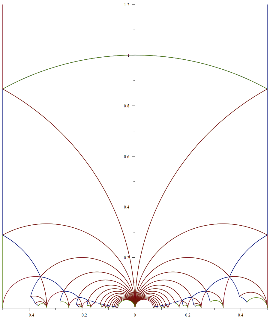
3. Some pictures and examples
We have implemented our fundamental domains on the computer algebra system Maple by drawing the ideal geodesic triangles. In Maple, the system decides that the edges of such triangles should have colors among red, blue and green. When the edges overlap, the priority is redbluegreen. As a result, the colors of the geodesic triangles in our fundamental domains are
Example 3.1.
We show a labeled picture of our fundamental domain for to assist in intuition of what regions are produced by our fundamental domains. Note that
where is the Euler totient function. Since , this is the same as .
Here the function for with is
| 0 | 2 | 3 | ||
| 1 | 0 | 0 | 1 |
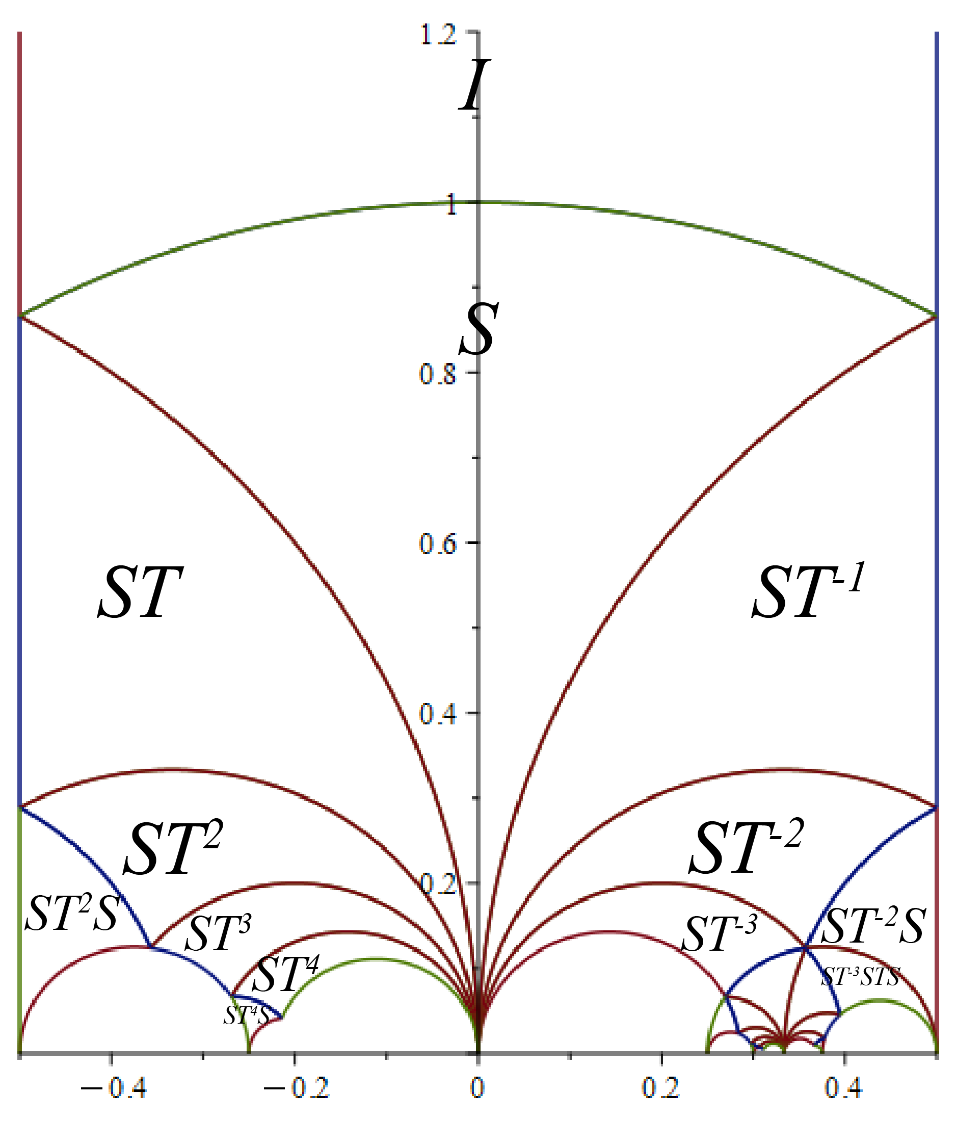
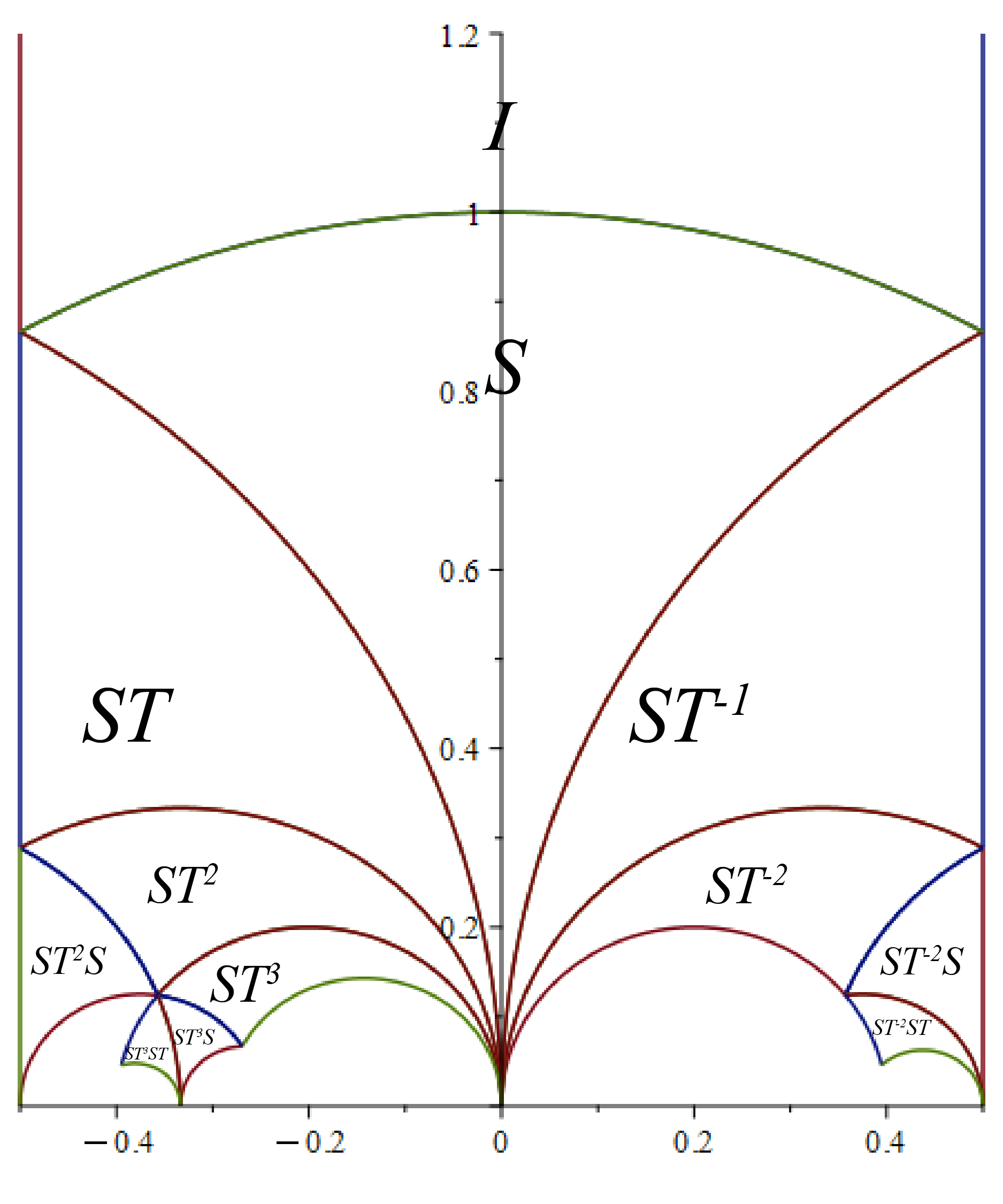
Example 3.2.
We show the fundamental domain for , with labels including a zoomed out and zoomed in version in order to fully label it in a readable fashion.
In this case, is always 0 for with as in Remark 2.23 since . The with is only with . Then , where . These numbers are observed in the picture as .
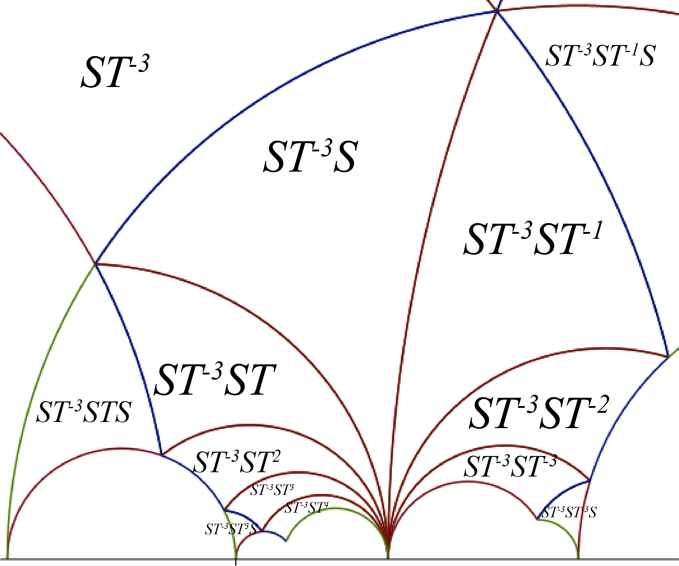
Example 3.3.
It may help to illustrate in detail our result for in the case of . We chose since it has three prime factors, so is the first example with by Remark 2.23.
The index [DS]* p. 21 is
Now has 30 elements. The number of nonunits with is . Each corresponds to a preferred with .
Now we concentrate on the classes with . We have of them. The following is a list of the elements in the equivalent classes, with and listed in the front.
| 1 | (, ) | {(2, 3), (14, ), (, 3), (, 9), (4, ), (8, ), (, 9), (, )} |
| 2 | (, ) | {(2, 5), (14, 5), (, ), (, 5), (4, ), (8, 5), (, ), (, )} |
| 1 | (4, 3) | {(2, 9), (14, 3), (, 9), (, ), (4, 3), (8, ), (, ), (, )} |
| 1 | (, 15) | {(2, 15), (14, 15), (, 15), (, 15), (4, 15), (8, 15), (, 15), (, 15)} |
| 1 | (, ) | {(2, ), (14, ), (, ), (, 3), (4, ), (8, 9), (, 3), (, 9)} |
| 1 | (, ) | {(2, ), (14, ), (, 5), (, ), (4, 5), (8, ), (, 5), (, 5)} |
| 2 | (, ) | {(2, ), (14, 9), (, ), (, ), (4, 9), (8, 3), (, ), (, 3)} |
| 1 | (3, 2) | {(3, 2), (, 14), (3, ), (9, ), (, 4), (, 8), (9, ), (, )} |
| 1 | (, ) | {(3, 4), (, ), (3, 14), (9, ), (, 8), (, ), (9, 2), (, )} |
| 2 | (3, 5) | {(3, 5), (, 5), (3, ), (9, 5), (, ), (, 5), (9, ), (, )} |
| 3 | (3, 8) | {(3, 8), (, ), (3, ), (9, 14), (, ), (, 2), (9, 4), (, )} |
| 1 | (, ) | {(3, 10), (, 10), (3, ), (9, 10), (, ), (, 10), (9, ), (, )} |
| 1 | (9, 8) | {(3, ), (, ), (3, ), (9, ), (, 2), (, 4), (9, 8), (, 14)} |
| 3 | (5, 14) | {(5, 2), (5, 14), (, ), (5, ), (, 4), (5, 8), (, ), (, )} |
| 2 | (5, 9) | {(5, 3), (5, ), (, 3), (5, 9), (, ), (5, ), (, 9), (, )} |
| 1 | (5, 4) | {(5, 4), (5, ), (, 14), (5, ), (, 8), (5, ), (, 2), (, )} |
| 1 | (, ) | {(5, 6), (5, 12), (, 6), (5, ), (, 12), (5, ), (, ), (, )} |
| 1 | (6, 5) | {(6, 5), (12, 5), (6, ), (, 5), (12, ), (, 5), (, ), (, )} |
| 1 | (10, 9) | {(10, 3), (10, ), (, 3), (10, 9), (, ), (10, ), (, 9), (, )} |
| 1 | (15, 14) | {(15, 2), (15, 14), (15, ), (15, ), (15, 4), (15, 8), (15, ), (15, )} |
Putting the information together, we see that for a nonunit , we have the following list.
| 0 | |
|---|---|
| 1 | |
| 2 | |
| 3 | 3, 5 |
The total number of with and is now
The corresponding cusp for in (2.21) is
and since , we see that this cusp happens for times. Therefore, we have the following table, where we also give which cusp representative each is equivalent to.
| 2 | 3 | 4 | 5 | 6 | 8 | 9 | 10 | 12 | 14 | 15 | |||||||||||
| cusp | |||||||||||||||||||||
| 1 | 4 | 2 | 4 | 2 | 1 | 2 | 2 | 1 | 1 | 2 | 2 | 1 | 1 | 2 | 2 | 1 | 2 | 3 | 2 | 3 | |
| cusp rep |
Here we compute the cusp representatives by [DS]*Prop 3.8.3, and their widths by [S]*Algorithm 1.19, summarized below.
| cusp rep | ||||||||
|---|---|---|---|---|---|---|---|---|
| width | 15 | 10 | 6 | 5 | 3 | 2 | 1 | 30 |
Note that the for our equivalent to a cusp representative add to its total width.
All these patterns can be observed nicely in our Figure 4.