Optimal and Stable Distributed Bipartite Load Balancing

We study distributed load balancing in bipartite queueing systems. Specifically, a set of frontends route jobs to a set of heterogeneous backends with workload-dependent service rates, with an arbitrary bipartite graph representing the connectivity between the frontends and backends. Each frontend operates independently without any communication with the other frontends, and the goal is to minimize the expectation of the sum of the latencies of all jobs. Routing based on expected latency can lead to arbitrarily poor performance compared to the centrally coordinated optimal routing. To address this, we propose a natural alternative approach that routes jobs based on marginal service rates, which does not need to know the arrival rates. Despite the distributed nature of this algorithm, it achieves effective coordination among the frontends. In a model with independent Poisson arrivals of discrete jobs at each frontend, we show that the behavior of our routing policy converges (almost surely) to the behavior of a fluid model, in the limit as job sizes tend to zero and Poisson arrival rates are scaled at each frontend so that the expected total volume of jobs arriving per unit time remains fixed. Then, in the fluid model, where job arrivals are represented by infinitely divisible continuous flows and service times are deterministic, we demonstrate that the system converges globally and strongly asymptotically to the centrally coordinated optimal routing. Moreover, we prove the following guarantee on the convergence rate: if initial workloads are $\delta$-suboptimal, it takes $\mathcal{O}(\delta+\log{1/\epsilon})$ time to obtain an $\epsilon$-suboptimal solution.

1 Introduction

This paper studies distributed load balancing in bipartite queueing systems. In many real-world applications such as data centers, cloud computing systems, and wireless networks, the systems often consist of multiple frontends (routers) that receive job requests and backends (servers) that process these jobs. A critical operational question is how to efficiently route jobs to the backends, namely, how to minimize the sum of the latencies experienced by jobs. Efficient resource management is becoming increasingly important given the growing demand for serving machine learning inference queries, which incur high latencies and require expensive computational resources.

We focus on distributed control as it offers several attractive features: 1) robustness: there is no single point of failure, 2) scalability: it is easy to add or remove frontends and backends, 3) reducing communication overhead: this is important due to privacy concerns and is critical for latency-sensitive service where communication delays can impact performance. These features are crucial for today’s large-scale service systems that require resilience and high performance.

Specifically, we consider a system where a set of frontends route jobs to a set of backends, with a general bipartite graph representing their connectivity. Due to various reasons including data residency regulations, geographical proximity, and job-server compatibility requirements, the frontends and backends do not necessarily form a complete graph. The backends have workload-dependent service rates, modeled as general functions of their workload. This modeling choice is motivated by the complexities of modern applications. Traditional many-server queue models represent the service process as a fixed number of identical processors, each processing one job at a time, working independently of one another. Hence, the rate at which the queue can process jobs increases linearly in the number of jobs requesting service, until every processor is occupied, at which point the processing rate does not increase at all. In backend systems for complex tasks like large language models inference, there is a high degree of parallelism but also contention for shared resources (e.g., bandwidth to various levels of the memory hierarchy, synchronization locks) leading to non-linearity in the processing rate as a function of total workload.

We model job arrivals to each frontend as independent Poisson processes. When a job arrives at a frontend, the frontend needs to decide which connected backend to route the job to. We allow general service distributions and only assume the number of job departures during each period equals the workload-dependent service rate in expectation. Jobs can be queued both at the frontends and at the backends, and we want the frontends to make routing decisions independently without communication among the frontends. The goal is to minimize expected latency, i.e., the total amount of time a job spends in the system.

1.1 Contributions

In this work, we study a distributed load balancing problem in a general bipartite queueing system with heterogeneous backends that has workload-dependent service rates. Routing the jobs to a connected backend with the shortest expected latency, though a natural idea, can lead to suboptimal outcomes. See Appendix A for a detailed discussion with Pigou’s Example (Pigou, 1920). We develop a simple distributed load balancing policy called the Greatest Marginal Service Rate policy (GMSR), which facilitates coordination among the frontends and achieves stability and asymptotic latency optimality under minimal assumptions on the problem setting. Our stability analysis introduces a novel Lyapunov function and relies on a combinatorial argument, which may be of independent interest.

A Simple Distributed Load Balancing Policy.

Motivated by the structure of the centrally coordinated optimal routing solution, we propose the GMSR policy as an alternative to routing based on expected latency. Under this policy, when a job arrives at a frontend, it is routed to a connected backend with the highest marginal service rate, i.e., the backend where an additional job would have the least impact on the overall service rate due to its current workload. GMSR enjoys the following advantages:

• Distributed control: each frontend only needs to know the marginal service rate at connected backends and does not need to communicate with each other.

• Stability and latency optimality: GMSR is shown to minimize the expected latency jobs experience in the large-system limit. Specifically, the system is globally strongly asymptotically stable, which means that, regardless of the system’s starting point (globally), every possible trajectory (strongly) converges to the equilibrium point over time (asymptotically). I.e., GMSR facilitates effective coordination among the frontends so that the system converges to the centrally coordinated optimal routing.

• Agnostic to arrival rates: GMSR does not need to know the arrival rates of the jobs to the frontends, in contrast to LP-based policies previously studied in the literature (e.g., Bassamboo et al. 2006).

• Generality: applicable to general bipartite graphs with heterogeneous arrival rates and heterogeneous backends with workload-dependent service rates. The system can also start with an arbitrary amount of workload. This makes our policy feasible for a variety of practical systems that feature complex data locality and job-server compatibility constraints.

• Convergence rate guarantee: if initial workloads are $\delta$-suboptimal, i.e., the absolute difference between the sum of the initial workloads and the sum of the optimal workloads is $\delta$, then it takes $\mathcal{O}(\delta+\log{1/\epsilon})$ time to obtain an $\epsilon$-suboptimal solution.

• Robust to bounded adversarial perturbations: our asymptotic optimality result continues to hold in a semi-random model where an adversary can arbitrarily tamper the parameters up to some finite point in time. More generally, when the centrally coordinated optimal routing shifts due to changes in arrival rates, bipartite graph topology, or service rates, the system in the fluid model will consistently chase the new optimal routing and we provide convergence rates to the new optimal routing. Exact convergence, however, may not be guaranteed if the optimal routing changes too rapidly, i.e., the system is continuously adjusting but not fully catching up.

The GMSR policy extends the celebrated Join-the-Shortest Queue policy (JSQ) that is extensively studied in the literature (see Section 2.2), and our results imply the asymptotic optimality of the JSQ for identical servers with general bipartite graph, which to the best of our knowledge, had not previously been established.

Moreover, our model allows jobs to be queued at both frontends and backends, i.e., we allow a mixture of input queueing (jobs are queued at the frontends), and output queueing (jobs are queued at the backends). As output queueing requires each arriving job to be assigned to backends immediately upon arrival, the space of controls allowed for an output-queueing system is a subset of the corresponding input-queueing systems. Nevertheless, GMSR, as an output-queueing policy, achieves asymptotic latency optimality. Thus, we demonstrate that we can control the output-queueing system as efficiently as the corresponding input-queueing system in the large-system limit as job sizes tend to zero and arrival rates increase correspondingly.

Comparison to Related Work.

Four key characteristics set the focus of this paper apart from the literature: (i) distributed control, (ii) general bipartite graph topology, (iii) asymptotic latency optimality of the proposed policy, and (iv) heterogeneous and state-dependent servers. Prior studies, which we overview in Section 2, often differ by focusing on throughput optimality (i.e., stability of the policy), employing centralized control, or considering parallel systems with identical servers.

1.2 Our Techniques

The main techniques and novelty of our analyses are summarized as follows.

• We show the discrete-time stochastic system dynamics converge in the large-system limit (Theorem 1).

  Specifically, we consider a sequence of systems in which we shrink the job size to zero and scale the arrival rates correspondingly. We show the absolute compactness of the system dynamics by 1) establishing the relative compactness of its compensator, i.e., the expectation of stochastic integrals, and 2) showing that the dynamics converge to this compensator. In the latter step, we apply Burkholder inequality to establish a uniform law of large numbers for triangular arrays of martingale differences. By the Arzela-Ascoli theorem, we thus have the existence of sub-sequential limits. Moreover, we leverage classical functional analysis results such as Banach-Alaoglu and Banach-Saks theorems to show the limit is a solution of a differential inclusion.

• We adopt differential inclusion to formalize the system dynamics in the fluid model.

  Differential inclusions generalize differential equations by allowing the derivative to belong to a set of possible values (Aubin and Cellina, 1984; Smirnov, 2022). Therefore, a differential inclusion is an ideal mathematical framework to capture the system dynamics under GMSR, where ties in the gradients can lead to multiple potential routing decisions. Throughout the paper, we will use marginal service rate and gradient interchangeably.

  As the centrally optimal routing solution is equivalent to the equilibrium point of the differential inclusion (Lemma 4), the asymptotic optimality of GMSR is equivalent to the stability of solutions to the differential inclusion.

• We design a novel Lyapunov function that depends on flow imbalance for stability analysis (Lemma 5).

  Specifically, the Lyapunov function is defined as the sum of absolute values of drifts at the backends, which physically represents the total flow imbalance (difference between job arrivals and service completion) in the system. This function not only depends on the system state (i.e., workloads) but also on internal algorithmic choice (i.e., routing decisions). Our Lyapunov function also implies the robustness of the system to bounded adversarial perturbations. Since the Lyapunov function is the sum of absolute values of drifts at the backends, any changes in system parameters—such as arrival rates, service rates, or the network topology—will be inherently accounted for. The system will always converge to the optimal fluid solution corresponding to the concurrent parameters.

  By showing this Lyapunov function consistently decreases over time, we demonstrate the global strong asymptotic stability of the system, i.e., regardless of the system’s initial state, every possible solution of the differential inclusion will converge to the equilibrium point over time (Theorem 2). The challenge of the analysis lies in the existence of equal-gradient hypersurfaces on which frontends need to decide how to break ties between connected backends with equal marginal service rates. For example, suppose there is one frontend connected to two backends. When one backend has a strictly higher marginal service rate, the system dynamics are uniquely determined. However, when both backends are equally favorable, the frontend can pick an arbitrary tie-breaking rule between them. This phenomenon is related to sliding mode control (Utkin, 2013), where the drifts are discontinuous at the sliding surface (the equal-gradient hypersurfaces in our problem), and the system dynamics on and around the sliding surface depend on various factors such as job arrival rates, local service rates, and their derivatives, and the graph structure.

• We present a combinatorial analysis of the system dynamics using the concepts of tier and TierGraph to show the value of the Lyapunov function always decreases.

  The notion of a “tier” (Definition 3) is used to capture the frontends’ routing decisions. Given the connectivity bipartite graph and a workload level, consider a subgraph with the edges connecting frontends with their most preferrable backends, i.e., with the highest gradients. A tier, consisting of a set of frontends and backends, is a connected component in this graph. The “TierGraph” (Definition 4) is a graphical representation of the original connectivity bipartite graph that captures the relationship between the tiers. Each tier is reduced to a vertex, and a vertex $v_{i}$, representing tier $i$, has an edge pointing to vertex $v_{j}$, representing tier $j$, if and only if there exists a frontend in tier $i$ that is connected with a backend in tier $j$. Thus, the reachability relation on the TierGraph reveals some fundamental facts about the relative order of gradient values of tiers.

  Note that the tiers and TierGraph change as the system state (i.e., workloads) changes. By analyzing the dynamics of them, we can understand how the system evolves over time. Specifically, we examine the implications of tiers that slide (workloads within the tier change while maintaining the tier structure), split (a tier divides into multiple tiers), and reconfigure (tiers merge or reorganize). Through this combinatorial analysis, we show that the Lyapunov function we constructed continues to decrease regardless of how the tiers change.

• We establish a two-phase convergence process for the total workloads approaching the optimal workloads, with the latter phase exponentially fast (Theorem 3).

  Notably, the Euclidean distance between the workloads and the optimal workloads need not decrease monotonically with time. Nevertheless, we show the sum of workloads at the backends converges as follows. The convergence can have two phases—the first phase may not be present depending on the initial system state. If the system starts with high workloads (which is made clear in Section 6.3), we show at least one backend’s workload decreases linearly. Within a finite time, the system will reach a stage where the Lyapunov function converges to zero exponentially fast. We show the absolute difference between the total workloads and the optimal workloads is bounded by the Lyapunov function, implying the exponential convergence of the total workloads. This two-phase process can be concisely summarized with a unified theorem: if initial workloads are $\delta$-suboptimal, it takes $\mathcal{O}(\delta+\log{1/\epsilon})$ time to obtain an $\epsilon$-suboptimal solution.

1.3 Organization of the Paper

The rest of the paper is organized as follows. In Section 2, we review related literature. Section 3 described the discrete-time model and the fluid relaxation problem. The GMSR policy is introduced in Section 4, and we present the convergence to the fluid model in Section 5. The stability analyses are in Section 6. Finally, we discuss the performance of GMSR in the original discrete-time model and conclude with further research directions. All proofs are deferred to the appendix.

2 Literature Review

We discuss two streams of work distinguished by where the jobs are queued: input queueing, where jobs are queued at the frontends, and output queueing, where jobs are queued at the backends.

2.1 Input Queueing Systems

Motivated by applications in call centers and manufacturing, there has been extensive literature on dynamic scheduling for parallel server systems aimed at minimizing costs such as holding costs, customer delay costs, and customer reneging costs.

These studies focus on asymptotically optimal dynamic scheduling policies under different heavy traffic regimes (Harrison and López, 1999; Mandelbaum and Stolyar, 2004; Bell and Williams, 2005; Anselmi and Casale, 2013; Atar, 2005; Tezcan and Dai, 2010; Atar et al., 2004; Ward and Armony, 2013; Bassamboo et al., 2006; Mandelbaum and Stolyar, 2004).

While these works provide valuable insights into scheduling policies that multiserver input-queued systems with multiple task types, they focus on input-queueing settings where jobs are queued at the frontends. Here the control is to pick which job to serve when a server becomes available. In our setting, the backends have workload-dependent service rates, it’s not clear when the backend is “available.” Thus the policies designed for input queueing systems have limited applicability in our setting.

2.2 Output Queueing Systems

Motivated by wireless networks, there have been extensive studies on distributed load balancing that aim to minimize latency and maximize throughput.

Join-the-Shortest Queue (JSQ) and Variants.

The JSQ policy, first described for a single-router model, directs jobs to the queue with the shortest line. Its optimality in minimizing the long-run average latency has been established under various conditions (Winston, 1977; Weber, 1978; Johri, 1989; Liu et al., 2022).

However, JSQ is not always optimal, even with identical servers and one router, see Whitt (1986) for counterexamples (e.g. service time distributions with large variance).

To address systems with heterogeneous servers, Chen and Ye (2012) generalize JSQ and show its asymptotic optimality in the heavy traffic regime, and Hurtado-Lange and Maguluri (2021) gives necessary and sufficient conditions for throughput and latency optimality.

JSQ can also be applied to systems with multiple routers in a distributed fashion, where each router sends jobs to the connected servers with the shortest queue. Foss and Chernova (1998) discusses sufficient conditions for stability, while Cruise et al. (2020) investigates stability in systems where task-server constraints are modeled as a hypergraph. Weng et al. (2020) consider the join-the-fastest-shortest-queue (JFSQ) and the join-the-fastest-idle-queue (JFIQ) policy and shows their asymptotic optimality, but they need the graph to be “well-connected.” The impact of connectivity constraints (also referred to as data locality) on the performance of routing policies is explored in Zhao et al. (2024); Cardinaels et al. (2022); Rutten and Mukherjee (2023). Stolyar (2005) proposes routing based on the queue length weighted by the inverse of the service rate, but their model does not incorporate state-dependent service rates, which are a key feature in our setting. For a comprehensive overview, readers may refer to Van der Boor et al. (2018). Our policy can be interpreted as “Join-the-Steepest Queue,” as the frontends send jobs to connected backends with the highest marginal service rate; and when we have identical servers, our policy is reduced to JSQ.

Similar to JSQ, Tezcan (2008) shows that Minimum-Expected-Delay Faster-Server-First and Minimum-Expected-Delay Load-Balancing (that balance the utilization of servers) are asymptotically optimal under the Halfin and Whitt regime for one router and heterogeneous servers.

Backpressure/MaxWeight Policy.

The classic backpressure policy (Tassiulas and Ephremides, 1990; Georgiadis et al., 2006) in a bipartite graph with output queueing (i.e., jobs are queued at the servers) can be reduced to JSQ. The backpressure policy will be mean rate optimal but not necessarily latency optimal in our setting. Neely (2022) proposes a drift-plus-penalty method that can be used to stabilize a queueing network while also minimizing the time average of a penalty function. However, since the penalty function depends only on the controller’s actions and not on the queue lengths, this method is not suitable for latency minimization in our setting. MaxWeight policies, when applied to input queueing systems, require centralized computation of a weighted bipartite matching (Stolyar, 2004; Maguluri et al., 2012), making them unsuitable for distributed control at the frontend side.

Other policies.

Round Robin (RR) policies have the advantage of requiring no state information. Hajek (1985) shows it minimizes average latency with one router and identical servers; Ye (2023) shows that for one router and heterogeneous servers, RR achieves the optimal performance asymptotically within the class of admissible policies that require no state information. Lastly, there is a stream of papers that study probabilistic assignment and pattern allocation (Combé and Boxma, 1994; Altman et al., 2000).

3 Problem Formulation

In this section, we introduce a discrete-time model for the load balancing problem with a bipartite queueing system. Consider a bipartite graph $\mathcal{G}=(\mathcal{F},\mathcal{B},\mathcal{E})$, where $\mathcal{F}$ is the set of frontends, $\mathcal{B}$ is the set of backends, and $\mathcal{E}$ is the set of edges connecting frontends to backends: if $(f,b)\in\mathcal{E}$ for $f\in\mathcal{F},b\in\mathcal{B}$, then frontend $f$ can route jobs to backend $b$, and we say $f$ and $b$ are connected. We denote by $\mathcal{F}(b)$ and $\mathcal{B}(f)$ the set of frontends connected to backend $b\in\mathcal{B}$ and the set of backends connected to frontend $f\in\mathcal{F}$, respectively. We do not assume the graph to be fully connected, and we only assume that no frontends or backends are isolated, i.e., $\mathcal{F}(b)\neq\emptyset$, $\mathcal{B}(f)\neq\emptyset$ for all $f\in\mathcal{F},b\in\mathcal{B}$.

In each period $n\geq 1$, the number of jobs arriving at frontend $f$ is a Poisson variable with rate $\lambda_{f}$, denoted by $W_{f}(n)$. Upon arrival, a job can either queue at the frontend or be sent to a connected backend for service. The job service rate at the backend $b\in\mathcal{B}$ is denoted by $\ell_{b}(N_{b})\geq 0$, which is a function of the workload $N_{b}$ at this backend $b$. Let $G_{f}(n)$ denote the number of jobs queued at frontend $f$ and let $N_{b}(n)$ denote the number of jobs at backend $b$ at time period $n$, the system dynamics are given by

$$G_{f}(n+1)=G_{f}(n)+W_{f}(n)-\sum_{b\in\mathcal{B}(f)}A_{f,b}(n),$$

$$N_{b}(n+1)=N_{b}(n)+\sum_{f\in\mathcal{F}(b)}A_{f,b}(n)-D_{b}(n),$$

where

• $A_{f,b}(n)$ denotes the number of arriving jobs routed from frontend $f$ to backend $b$, and the total number of jobs routed from frontend $f$ cannot exceed the total number of jobs queueing there, i.e., $\sum_{b\in\mathcal{B}(f)}A_{f,b}(n)\leq G_{f}(n)+W_{f}(n)$.

• $D_{b}(n)$ denotes the number of jobs departures from backend $b$, which satisfies $\mathbb{E}[D_{b}(n)]=\ell_{b}(N_{b}(n))$ and $D_{b}(n)\leq N_{b}(n)$.

The decision-maker needs to design an online policy that routes arriving jobs to the backends to minimize the long-run average latency each job experiences. If the system can be stabilized, i.e., the workload does not explode, then we can apply Little’s Law, which implies the objective is equivalent to minimizing the long-run average number of jobs in the system.

Let $\pi$ denote any online policy for our load balancing problem, then the long-run average number of jobs in the system under policy $\pi$ is defined as

$$\limsup_{n\to\infty}\frac{1}{n}\mathbb{E}_{\pi}\left[\sum_{k=1}^{n}\left(\sum_{f\in\mathcal{F}}G_{f}(k)+\sum_{b\in\mathcal{B}}N_{b}(k)\right)\right],$$

where the expectation is taken over the arrival process, job service process, and the probability measure induced by the policy $\pi$.

To analyze the performance of a policy $\pi$, we benchmark against the fluid relaxation of the problem. The fluid optimization problem can be formulated as follows:

$$\textsf{OPT =}\min_{\bm{N},\bm{x}}\quad \sum_{b\in\mathcal{B}}N_{b}$$ (1)

s.t. $$\sum_{f\in\mathcal{F}}\lambda_{f}x_{f,b}=\ell_{b}(N_{b}),\forall b\in\mathcal{B},$$

$$\sum_{b\in\mathcal{B}}x_{f,b}=1,\forall f\in\mathcal{F},$$

$$x_{f,b}\geq 0,\forall(f,b)\in\mathcal{E},$$

$$x_{f,b}=0,\forall(f,b)\notin\mathcal{E},$$

where $N_{b}$ denotes the steady-state load level at each backend $b\in\mathcal{B}$, and $x_{f,b}$ for $(f,b)\in\mathcal{E}$ denotes the proportion of jobs that is sent from frontend $f$ to backend $b$. The first constraint imposes flow balance at each backend, i.e., at the equilibrium point, the total flow into backend $b$, $\sum_{f\in\mathcal{F}}\lambda_{f}x_{f,b}$ equals the total flow out of backend $b$, $\ell_{b}(N_{b})$. The second constraint imposes flow balance at each frontend, i.e., all jobs are sent to backends. The last two sets of constraints impose the connectivity constraints.

We conduct our analysis under the following assumptions.

Assumption 1.

The service rate functions $\{\ell_{b}\}_{b\in\mathcal{B}}$ are strictly increasing, strictly concave, bounded, and twice continuously differentiable, with $\ell_{b}(0)=0$.

Service rates are non-decreasing because higher loads lead to higher service rates: the service rate never decreases when new jobs arrive because the backend always has the option to delay working on those jobs and continue processing the ones that were already in progress. Concavity reflects decreasing returns to scale: the available resources to process the next-arriving job are a decreasing function of the number of jobs already being served. When the workload is zero, so is the service rate. We assume boundedness to reflect the finite capacity of real-world systems. Twice continuous differentiability and strict concavity are technical assumptions to simplify the analysis. The assumption that service rate functions are strictly increasing is a direct consequence of strict concavity combined with non-decreasingness.

Assumption 2.

The optimization problem (1) is feasible.

The feasibility assumption is necessary for the system to be stable, i.e., the service capacity of the backends is enough to serve all arriving jobs without allowing the queue sizes to explode. A necessary and sufficient condition is the existence of workloads such that for every subset of frontends their total arrival rates is weakly smaller than the service rate of their connected backends. Feasibility also guarantees the existence of an optimal solution as the feasible set is non-empty and closed, and the objective function is continuous and coercive over the feasible set.

An important result connecting the performance of any online policy and the optimal fluid relaxation is given by the following lemma.

Lemma 1.

For any online policy $\pi$,

$$\mathsf{OPT}\leq\limsup_{n\to\infty}\frac{1}{n}\mathbb{E}_{\pi}\left[\sum_{k=1}^{n}\left(\sum_{f\in\mathcal{F}}G_{f}(k)+\sum_{b\in\mathcal{B}}N_{b}(k)\right)\right].$$

This lemma establishes that the fluid optimal solution provides a lower bound on the performance of any online policy. It holds for all online policies, regardless of whether they are centralized or distributed. The proof relies on identifying the following necessary condition for the system to be stable (i.e., the workloads do not explode): for any subset of frontends, the total arrival rates should be at most the total service rates of all connected backends at the long-run average workload level. When this necessary condition holds, we use max-flow-min-cut to show that the induced long-run average workload is a feasible solution to an optimization problem that has the same optimal solution to the fluid optimization problem (1).

Next, we explore two properties of the optimal solution to the fluid optimization problem.

Lemma 2.

The optimal $\bm{N}^{*}$ to the fluid optimization problem (1) is unique.

The uniqueness of the optimal workload holds as the service rate functions are strictly increasing and strictly concave, and we prove this by contradiction. Note that the optimal flow assignment $\bm{x}^{*}$ could be non-unique if the graph has cycles because we can always push flow through a circulation without changing the objective value.

Lemma 3.

Let $(\bm{N},\bm{x})$ denote a feasible solution to the fluid optimization problem (1), then $(\bm{N},\bm{x})$ is optimal if and only if for each frontend $f\in\mathcal{F}$ there exists a constant $c_{f}$ such that for $b\in\mathcal{B}(f)$ we have $1/\ell_{b}^{\prime}(N_{b})\geq c_{f}$ with equality holding if $x_{f,b}>0$.

This lemma motivates our GMSR policy, as we explain in detail in the next section.

4 Greatest Marginal Service Rate Algorithm and System Dynamics

Lemma 3 implies that for any two backends $b_{1},b_{2}$ connected to the same frontend $f$, if the optimal proportions of jobs sent to them are positive, i.e., $x_{f,b_{1}}^{*}>0,x_{f,b_{2}}^{*}>0$, then their service rate gradients at the optimal workloads must be equal:

$$\ell^{\prime}_{b_{1}}({N_{b_{1}}^{*}})=\ell^{\prime}_{b_{2}}({N_{b_{2}}^{*}}).$$

Motivated by this observation—the gradients of service rate functions are balanced in the optimal solution—we consider the following policy, which we refer to as the Greatest Marginal Service Rate policy (GMSR): when a job arrives at a frontend, send it to a connected backend with the highest gradient $\ell_{b}^{\prime}(N_{b})$. In this algorithm, frontends make independent decisions without communication with each other, and each frontend only needs to know the workloads at its connected backends. Notably, the algorithm does not require knowledge of the job arrival rates $\{\lambda_{f}\}_{f\in\mathcal{F}}$.

Mathematically, frontends send jobs to a connected backend with the highest gradient, i.e., for all $f\in\mathcal{F}$ we pick $\bm{x}_{f}\in X_{f}(\bm{N})$ where

$$X_{f}(\bm{N}):=\arg\max \sum_{b\in\mathcal{B}(f)}{x_{f,b}}{\ell^{\prime}_{b}(N_{b})}$$ (2)

s.t. $$\sum_{b\in\mathcal{B}}x_{f,b}=1,$$

$$x_{f,b}\geq 0,\forall(f,b)\in\mathcal{E},$$

$$x_{f,b}=0,\forall(f,b)\notin\mathcal{E}.$$

Here $x_{f,b}$ represents the proportions of jobs routing from frontend $f$ to backend $b$. It is important to note that the system dynamics under GMSR may not be uniquely determined at all times due to potential ties in the gradients $\ell^{\prime}_{b}(N_{b})$. Thus, $X_{f}(\bm{N})$ is a set-valued function.

We remark that GMSR can break ties between backends in any way and how ties are broken in the discrete-time stochastic system does not impact our analysis. For example, if there is one frontend connected to two backends and $\ell_{1}^{\prime}(N_{1}(n))=\ell_{2}^{\prime}(N_{2}(n))$, then the feasible proportion of jobs that are sent to the two backends can be anything as long as $x_{1,1}(n)+x_{1,2}(n)=1,x_{1,1}(n),x_{1,2}(n)\geq 0$.

Given the routing decisions, the system dynamics under GMSR is given by

$$N_{b}(n+1)=N_{b}(n)+\sum_{f\in\mathcal{F}(b)}A_{f,b}(n)-D_{b}(n),$$

where

• $A_{f,b}(n)$ denotes the number of arriving jobs routed from frontend $f$ to backend $b$, which satisfies $\mathbb{E}[A_{f,b}(n)]=\lambda_{f}x_{f,b}(n)$ with $\bm{x}_{f}(n)\in X_{f}(\bm{N}(n))$, and $\sum_{b\in\mathcal{F}(b)}A_{f,b}(n)$ follows a Poisson distribution with rate $\lambda_{f}$.

• $D_{b}(n)$ denotes the number of jobs departures from backend $b$, which satisfies $\mathbb{E}[D_{b}(n)]=\ell_{b}(N_{b}(n))$ and $D_{b}(n)\leq N_{b}(n)$.

5 Convergence to the Fluid Model

In this section, we show that the discrete system dynamics under GMSR converge to a fluid model in a large-system limit in which we shrink the job size to zero and scale the arrival rates correspondingly. In this fluid model, jobs are modeled as infinitely divisible continuous flows and there is no stochasticity in arrivals or service times.

To formalize this, fix a time horizon $T>0$, and consider a sequence of discrete systems indexed by a “system size” parameter $(c)$ whose dynamics within time interval $[0,T]$ are as follows:

$$N_{b}^{(c)}(n+1) =N_{b}^{(c)}(n)+\sum_{f\in\mathcal{F}(b)}A_{f,b}^{(c)}(n)-D_{b}^{(c)}(n),$$

where

• $n$ is the index of the discrete time step, each time step has a physical time length of $1/c$ in the $c^{th}$ system. Hence $n$ ranges over $\{0,1,\ldots,\lfloor T/c\rfloor\}$;

• $A^{(c)}_{f,b}(n)$ satisfies $\mathbb{E}[A^{(c)}_{f,b}(n)]=\lambda_{f}x^{(c)}_{f,b}(n)$ with $\bm{x}^{(c)}_{f}(n)\in X_{f}(\bm{N}^{(c)}(n)/c)$, and $\sum_{b\in\mathcal{F}(b)}A^{(c)}_{f,b}(n)$ follows a Poisson distribution with rate $\lambda_{f}$.

• $D_{b}^{(c)}(n)$ satisfies $\mathbb{E}[D_{b}^{(c)}(n)]=\ell_{b}(N_{b}^{(c)}(n)/c)$, $D_{b}^{(c)}(n)\leq N_{b}^{(c)}(n)$, and

  $$\sup_{c}\sup_{1\leq n\leq Tc}\mathbb{E}[(D_{b}^{(c)}(n))^{4}]<\infty.$$

The stochastic recursion given above is often referred to as a stochastic recursive inclusion. Note that we do not need the number of jobs sent from frontend $f$ to backend $b$, i.e., $A_{f,b}^{(c)}(n)$, to follow a Poisson distribution. When jobs arrive at the frontend, the frontend can 1) break ties arbitrarily as long as it picks the most preferable connected backends and 2) upon picking $\bm{x}^{(c)}_{f}$, the frontend can implement this routing proportion in any way as long as the number of jobs distributed follows $\bm{x}^{(c)}_{f}$ in expectation. For example, the control can be implemented in a weighted round-robin or probabilistic fashion. As for job departures, we allow general service distributions and only require the fourth moment to be uniformly bounded across time and system scale.

Our scaling shrinks the length of each time step and the size of jobs by a factor of $1/c$, and we will scale $c$ to infinity. Let $Y_{b}^{(c)}(n):=N_{b}^{(c)}(n)/c$ for all $b\in\mathcal{B}$. To analyze the convergence, let $t$ denote the physical time index, which should be distinguished from the algorithmic discrete time step index $n$. Specifically, in the $c^{th}$ system, the physical time for one discrete time step is $1/c$, thus the time point after $n$ steps is $n/c$. On the other hand, given time $t>0$, the number of steps passed is given by $\lceil tc\rceil$.

We construct a continuous piecewise-linear interpolation $\bar{\bm{Y}}^{(c)}(t)$ of the discrete process ${\bm{Y}}^{(c)}(n)$ over $t\in[0,T]$, where $\bar{\bm{Y}}^{(c)}(n/c)=\bm{Y}^{(c)}(n),n\geq 0$, and

$$\bar{\bm{Y}}^{(c)}(t)=\bm{Y}^{(c)}(n)+\left(\bm{Y}^{(c)}(n+1)-\bm{Y}^{(c)}(n)\right)\frac{t-n/c}{1/c},t\in[n/c,(n+1)/c].$$

With some abuse of notation, we use the argument to refer both to the discrete step index in ${\bm{Y}}^{(c)}(n)$ and the physical time index in $\bar{\bm{Y}}^{(c)}(t)$.

Our convergence result is as follows.

Theorem 1.

Almost surely, the set of sub-sequential limits of $\{\bar{\bm{Y}}^{(c)}(\cdot)\}$ as $c\to\infty$ is non-empty in the space of continuous functions with the uniform norm topology $C([0,T],\mathbb{R}^{|\mathcal{B}|})$, and for every such limit point $\bm{N}(\cdot)$, there exists $\bm{x}_{f}(t)\in X_{f}(\bm{N}(t))$ for all $f\in\mathcal{F}$, $t\in[0,T]$ such that $\bm{N}(\cdot)$ satisfies

$$N_{b}(t)=N_{b}(0)+\int_{0}^{t}\left(\sum_{f\in\mathcal{F}(b)}\lambda_{f}x_{f,b}(\tau)-\ell_{b}(N_{b}(\tau))\right)\,d\tau\text{ for all }b\in\mathcal{B},t\in[0,T].$$

The proof is built on Theorem 5.2 of Borkar (2008) and Theorem 3.7 of Duchi and Ruan (2018), who study stochastic recursive inclusions. The main difference is that they consider diminishing time step sizes and analyze the system behavior as time goes to infinity; our results focus on a sequence of systems indexed by $c$ and examine the system behavior as $c$ goes to infinity. This shift necessitates the analysis of a uniform law of large numbers for triangular arrays of martingale differences, which we prove using Burkholder inequality (see Lemma 19). The proof has two steps. Firstly, we use our uniform law of large numbers to show that the stochastic process $\{\bar{\bm{Y}}^{(c)}(\cdot)\}_{c\in\mathbb{N}}$ converges uniformly to its compensator, i.e., the integral of its drift. Because the compensator is equicontinous, we can use the Arzela-Ascoli theorem to extract a converging subsequence, which implies, in turn, the relative compactness of the original process $\{\bar{\bm{Y}}^{(c)}(\cdot)\}_{c\in\mathbb{N}}$. Secondly, we apply some functional analysis results to show that every limit point is a solution to the differential inclusion.

Remark 1.

Note that $\bm{x}_{f}(t)\in X_{f}(\bm{N}(t))$ is a set-valued function due to the potential non-uniqueness of optimal routing decisions when gradients are tied, thus the limit point $\bm{N}(\cdot)$ is a solution to a differential inclusion, which is a mathematical formulation that generalizes differential equations to allow the derivative to belong to a set of possible values (for details, see Aubin and Cellina 1984; Smirnov 2022). Specifically, the dynamics of the limit is defined by:

$$\dot{\bm{N}}(t)\in H(\bm{N}(t)),$$ (3)

where

$$H(\bm{N}):=\left\{(v_{1},\ldots,v_{|\mathcal{B}|}):v_{b}=\sum_{f\in\mathcal{F}(b)}\lambda_{f}x_{f,b}(t)-\ell_{b}(N_{b}(t)),\bm{x}_{f}\in X_{f}(\bm{N}),\forall f\in\mathcal{F},b\in\mathcal{B}\right\}.$$ (4)

Theorem 1 shows the stochastic recursive inclusion can be interpreted as a noisy discretization of a solution of the differential inclusion (3), i.e., $\{\bar{\bm{Y}}^{(c)}\}$ “track” a solution $\bm{N}(\cdot)$ with probability 1. In addition, Theorem 1 implies the existence of an absolutely continuous solution to the differential inclusion (3) on $[0,T]$. For proof of the existence of the global solution, i.e., on $[0,\infty)$, see Appendix C.1.

While the differential inclusion allows for arbitrary tie-breaking in routing decisions, the set of feasible routing decisions in a solution to the differential inclusion is in fact quite constrained by the requirement that the solution be absolutely continuous. This is due to the self-correcting feature of the algorithm. For instance, consider a scenario with one frontend and two identical backends, both starting with zero workloads. If the frontend initially routes unequal flows to the backends, the backend receiving more flow will accumulate more workloads, resulting in a lower gradient and making it less attractive to the frontend. When jobs are discrete, the system state will oscillate around the equal-gradient curve, where both backends have the same gradient (see Appendix F for simulations). However, in the fluid model, when we model jobs as infinitely divisible continuous flows, the system always stays on the equal gradient curve. To do so, in the one-frontend-two-backends example, the differential inclusion must pick the unique routing proportions $(x_{1,1}(t),x_{1,2}(t))\in X_{1}((N_{1}(t),N_{2}(t)))$ that produce a drift tangent to the equal-gradient curve. The routing proportions $\bm{x}_{1}(t)$ in the differential inclusion can be interpreted as a “local” time-average of the routing proportions $\bm{x}_{1}^{(c)}(n)$ of the stochastic recursive inclusion.

In the following lemma, we connect the equilibrium point of the dynamical system (3) with the optimal solution to the fluid optimization problem.

Lemma 4.

The dynamic system (3) has a unique equilibrium point $\bm{N}^{eq}$, which is optimal for the fluid optimization problem (1).

Therefore, the equilibrium point of the dynamic system (3) is equivalent to the unique optimal solution to the fluid optimization problem (1), and we will refer to it as $\bm{N}^{*}$ in the remainder of the paper.

6 Stability and Convergence Rate Analyses

In the previous section, we establish the convergence result, and that the equilibrium of the differential inclusion corresponds to the optimal fluid solution. We now analyze the stability of this equilibrium and the convergence rate to this equilibrium, which then implies that GMSR is asymptotically optimal and achieves effective coordination in the fluid model. Specifically, we show that $\bm{N}^{*}$ is globally strongly asymptotically stable, i.e., regardless of the system’s starting point (globally), every possible trajectory or solution (strongly) of the differential inclusion will converge to the equilibrium point over time (asymptotically), as time approaches infinity.

Definition 1.

The equilibrium position $\bm{N}^{*}$ of differential inclusion (3) is said to be globally strongly asymptotically stable if each solution $\bm{N}(\cdot)$ of the differential inclusion (3) with any initial state $\bm{N}(0)$ satisfies

$$\lim_{t\to\infty}\bm{N}(t)=\bm{N}^{*}.$$

Our main results are the following two theorems.

Theorem 2 (Stability).

The equilibrium position $\bm{N}^{*}$ of the differential inclusion (3) is globally strongly asymptotically stable.

Theorem 3 (Convergence Rate).

If initial workloads are $\delta$-suboptimal $(\delta>0)$, i.e.,

$$\left|\sum_{b\in\mathcal{B}}N_{b}(0)-\sum_{b\in\mathcal{B}}N_{b}^{*}\right|=\delta,$$

it takes $\mathcal{O}(\delta+\log{1/\epsilon})$ time to obtain an $\epsilon$-suboptimal solution ($\epsilon>0$).

To prove the stability result, we use the Lyapunov direct method. Specifically, we construct a function that serves as a measure of the system’s “energy,” which is zero at the equilibrium point $\bm{N}^{*}$, and demonstrate this function consistently decreases over time. The Lyapunov function is formally defined in Section 6.1.

To prove the convergence rate result, we notice that the drift of the Lyapunov function restricted to a subset of backends with the same gradient is proportional to the Lyapunov function itself and the gradient of these backends. Therefore, if the gradients can be lower bounded by a constant, the Lyapunov function will converge exponentially fast. We define a set of system states in which gradients are uniformly bounded from below and show it is an invariant set, i.e., once the system reaches the set, it stays there forever. Then, we argue that the system state reaches this invariant set in linear time if starting outside, which gives our two-phase convergence process. We remark that the constants in the convergence rate can depend on the initial workloads and the initial parameters (the arrival rates, service rate functions, and compatibility graph).

The proofs for the following results, however complicated in the form, all rely on a simple yet powerful observation: frontends always send jobs to the most preferable connected backends. If a backend with a very high marginal service rate is not receiving jobs from a frontend, then either they are not connected, or the frontend is connected to another backend with an even higher marginal service rate.

Our analysis of the performance of GMSR primarily focuses on the fluid model. Back to the discrete model, the system may not converge precisely to the centrally coordinated optimal routing due to stochasticity and may oscillate around the optimal solution. The extent to which it oscillates should decrease as we scale the system size (see Appendix F for simulation results) and we leave the analyses of the discrete model with finite $c$ for future work.

6.1 Preliminaries

The next lemma introduces the Lyapunov function and proves its positive definiteness. Recall the system state at time $t$ is $\bm{N}(t)=(N_{1}(t),N_{2}(t),\ldots,N_{|\mathcal{B}|}(t))$, the workloads at each backend at time $t$, and the system dynamics follows $\dot{N}_{b}(t)=\sum_{f\in\mathcal{F}(b)}\lambda_{f}x_{f,b}(t)-\ell_{b}(N_{b}(t))$, where $\bm{x}_{f}(t)=(x_{f,1}(t),\ldots,x_{f,|\mathcal{B}|}(t))\in X_{f}(\bm{N}(t))$ for $f\in\mathcal{F}$. Let $\bm{x}(t)$ denote the matrix $\{x_{f,b}(t)\}_{f\in\mathcal{F},b\in\mathcal{B}}$.

Lemma 5.

The function $V(\bm{N},\bm{x})=\sum_{b\in\mathcal{B}}\left|\sum_{f\in\mathcal{F}(b)}\lambda_{f}x_{f,b}-\ell_{b}(N_{b})\right|$ is positive definite, i.e., $V(\bm{N},\bm{x})\geq 0$ for all $\bm{N},\bm{x}$ and for all $\bm{x}_{f}\in X_{f}(\bm{N})$ we have

$$V(\bm{N},\bm{x})=0\text{ if and only if }(\bm{N},\bm{x})=(\bm{N}^{*},\bm{x}^{*}),$$

where $\bm{x}^{*}$ satisfies $\sum_{f\in\mathcal{F}(b)}\lambda_{f}x_{f,b}^{*}-\ell_{b}(N_{b}^{*})=0$ for all $b\in\mathcal{B}$.

We next introduce some definitions that are based on workloads, $\bm{N}$, at the backends.

Definition 2 (Best Backend Graph).

Given a connectivity bipartite graph $\mathcal{G}=(\mathcal{F},\mathcal{B},\mathcal{E})$ and workloads at the backends $\bm{N}$, we define the best backend graph at $\bm{N}$ to be a subgraph of the original graph $\mathcal{G}$ that involves only those edges that connect each frontend $f$ to its most preferable backends according to $\ell_{b}^{\prime}(N_{b})$. Mathematically,

$${G}(\bm{N})=(\mathcal{F},\mathcal{B},{E}(\bm{N}))\text{ with }{E}(\bm{N})=\{(f,b)\in\mathcal{E}|b\in S_{f}(\bm{N})\},$$

where $S_{f}(\bm{N})=\{b\in\mathcal{B}(f)|\ell_{b}^{\prime}(N_{b})=\max_{j\in\mathcal{B}(f)}\ell_{j}^{\prime}(N_{j})\}$ is the set of best backends for frontend $f\in\mathcal{F}$ at $\bm{N}$.

Figure 1: A connectivity bipartite graph with four frontends (left side) and five backends (right side) with edges denoting feasible flow routing.

Figure 2: The best backend graph given a connectivity bipartite graph as shown in Figure 2 at a system state $\bm{N}$ with $\ell_{1}^{\prime}(N_{1})=3,\ell_{2}^{\prime}(N_{2})=2,\ell_{3}^{\prime}(N_{3})=1,\ell_{4}^{\prime}(N_{4})=2,\ell_{5}^{\prime}(N_{5})=3$.

Figure 3: A connectivity bipartite graph from Figure 2 rearranged with solid edges denoting that the frontend $f$ is connected to a best backends in $S_{f}(\bm{N})$ and dashed edges denoting connected but not best backends. The system state $\bm{N}$ is the same as in Figure 2.

Figure 4: The TierGraph $\mathcal{T}(\bm{N})$ at $\bm{N}$ that corresponds to the graph in Figure 2. Here the tiers are $(\{f_{1},f_{4}\},\{b_{1},b_{5}\}),(\{f_{2}\},\{b_{2}\}),(\{f_{3}\},\{b_{4}\})$ and $(\emptyset,\{b_{3}\})$, which corresponds to $v_{1},v_{2},v_{3},v_{4}$ respectively in the TierGraph.

Definition 3 (Tier).

We say that $(F,B)$ with $F\subseteq\mathcal{F},B\subseteq\mathcal{B}$ is a tier at $\bm{N}$ if

• $F\cup B$ is connected in the best backend graph ${G}(\bm{N})$,

• for all frontends $f\in F$ there is no backend $b\in\mathcal{B}\setminus B$ such that $(f,b)\in{E}(\bm{N})$,

• for all backends $b\in B$ there is no frontend $f\in\mathcal{F}\setminus F$ such that $(f,b)\in{E}(\bm{N})$.

In graph theory, the above definition is equivalent to say $F\cup B$ is the node set of a connected component of the best backend graph $G(\bm{N})$. Note that $F$ can be an empty set for a tier, and this will happen when $B=\{b\}$ with $b\notin\cup_{f\in\mathcal{F}}S_{f}(\bm{N})$, i.e., no frontend finds the backend preferable. On the other hand, $B$ can never be an empty set as $\mathcal{B}(f)\neq\emptyset$ for all $f\in\mathcal{F}$, thus every frontend will find at least one backend preferable. By definition, all backends in the same tier share the same gradient value, so we let $\ell^{\prime}_{B}(\bm{N})$ denote $\ell_{b}^{\prime}(N_{b})$ for $b\in B$ at $\bm{N}$.

Definition 4 (TierGraph).

Let $k(\bm{N})$ denote the number of disjoint tiers at $\bm{N}$, a TierGraph $\mathcal{T}(\bm{N})$ at $\bm{N}$ is defined as follows:

• the graph has $k(\bm{N})$ vertices, with each vertex $v_{i}$ representing a tier $(F_{i},B_{i})$ at $\bm{N}$,

• there is an arc pointing from vertex $v_{i}=(F_{i},B_{i})$ to vertex $v_{j}=(F_{j},B_{j})$ ($i\neq j$), which is denoted as $v_{i}\to v_{j}$, if there exists $f\in F_{i}\cap B_{j}$ such that $(f,b)\in\mathcal{E}$, i.e., they are connected in the connectivity bipartite graph $\mathcal{G}=(\mathcal{F},\mathcal{B},\mathcal{E})$.

We say $(F_{i},B_{i})\prec(F_{j},B_{j})$ if vertex $v_{i}$ can reach vertex $v_{j}$ in $\mathcal{T}(\bm{N})$.

For an example of tiers and TierGraph, please refer to Figure 4 and Figure 4. In the remainder of the paper, we denote the vertices in the TierGraph and their corresponding tiers using the same index. We next present some fundamental facts about the structure of the TierGraph and how the reachability relation on the TierGraph reveals the relative order of gradient values of tiers.

Lemma 6.

For two tiers $(F_{i},B_{i}),(F_{j},B_{j})$ with $F_{i},F_{j}\subseteq\mathcal{F},B_{i},B_{j}\subseteq\mathcal{B}$ at $\bm{N}$, let vertex $v_{i}$ and vertex $v_{j}$ denote their corresponding vertices in the TierGraph $\mathcal{T}(\bm{N})$. If $v_{i}\to v_{j}$, then $\ell_{B_{i}}^{\prime}(\bm{N})>\ell_{B_{j}}^{\prime}(\bm{N})$.

Corollary 1.

For two tiers $(F_{i},B_{i}),(F_{j},B_{j})$ with $F_{i},F_{j}\subseteq\mathcal{F},B_{i},B_{j}\subseteq\mathcal{B}$ at $\bm{N}$, if $(F_{i},B_{i})\prec(F_{j},B_{j})$, then $\ell_{B_{i}}^{\prime}(\bm{N})>\ell_{B_{j}}^{\prime}(\bm{N})$.

Corollary 2.

The TierGraph $\mathcal{T}(\bm{N})$ is a directed acyclic graph.

6.2 Stability Analysis

We proceed to prove the stability of the solution to the differential inclusion (3). There are two steps of the proof:

1. We show that if there exists a tier that does not change for a time interval, the workloads at the backends in this tier must all increase or all decrease, depending on the total flow imbalance within the tier (see Lemma 7). Specifically, when the total arrival rates exceed the total service rates, the workloads will increase and vice versa. We also establish flow imbalance inequalities for any subset of the tier, which will be used in the second step (see Lemma 8 and Lemma 9).

2. We next analyze the Lyapunov function. When the tiers do not change for a time interval, we show its value is the sum of absolute values of total flow imbalance within each tier, which decreases with time (see Lemma 10). When the tiers change, we show the value of the Lyapunov function still decreases (see Lemma 11 and Lemma 12) by analyzing how the tiers change, which relies on some fundamental structural properties of the TierGraph established in the previous section.

6.2.1 Analysis of a Tier’s Dynamics

First, we show that within a tier, the workloads of the backends evolve in the same direction. This is because, by definition, all backends in the same tier will share the same marginal service rate. Therefore to stay in the same tier, their gradients must remain aligned, and so are the workloads.

Lemma 7.

If there exists $t_{1}<t_{2}$ and $F\subseteq\mathcal{F},B\subseteq\mathcal{B}$ such that $(F,B)$ is a tier at $\bm{N}(t)$ for $t\in[t_{1},t_{2}]$, then for any $b_{1},b_{2}\in B$, $\frac{d}{dt}N_{b_{1}}(t)\cdot\frac{d}{dt}N_{b_{2}}(t)\geq 0$ for $t\in[t_{1},t_{2}]$.

Next, we establish flow imbalance inequalities for subsets of a tier, which are critical for analyzing the Lyapunov function. Within a tier, when the total arrival rates are higher than the total service rates, which we refer to as having “positive flow imbalance,” jobs arrive faster than jobs depart and the workload at every backend must increase. Locally, we prove each backend must experience positive flow imbalance too, i.e., in-flow dominates out-flow, and for this to be feasible, the flow imbalance inequalities for any subset of backends and their connected frontends in the tier must also hold. This result leverages that backends are sliding in their equal-gradient hypersurface.

Lemma 8.

If there exists $t_{1}<t_{2}$ and $F\subseteq\mathcal{F},B\subseteq\mathcal{B}$ such that for $t\in[t_{1},t_{2}]$,

• $(F,B)$ is a tier at $\bm{N}(t)$,

• $\sum_{f\in F}\lambda_{f}-\sum_{b\in B}\ell_{b}(N_{b}(t))\geq 0$.

Then for $t\in[t_{1},t_{2}]$, the following holds:

• $N_{b}(t)$ is non-decreasing in $t$ for all $b\in B$,

• for any subset of backends $Q\subseteq B$,

  $$\sum_{f\in F\cap(\cup_{b\in Q}\mathcal{F}(b))}\lambda_{f}\geq\sum_{b\in Q}\ell_{b}(N_{b}(t)).$$

Similarly, we have the following results for the “negative flow imbalance” case, i.e., when the total arrival rates are lower than the total service rates. In this case, jobs arrive slower than jobs depart, so the workloads at the backends must decrease. This implies similar local inequalities for any subset of frontends and their connected backends in the tier.

Lemma 9.

If there exists $t_{1}<t_{2}$ and $F\subseteq\mathcal{F},B\subseteq\mathcal{B}$ such that

• $(F,B)$ is a tier at $\bm{N}(t),t\in[t_{1},t_{2}]$,

• $\sum_{f\in F}\lambda_{f}-\sum_{b\in B}\ell_{b}(N_{b}(t))\leq 0$.

Then for $t\in[t_{1},t_{2}]$, the following holds:

• $N_{b}(t)$ is non-increasing in $t$ for all $b\in B$,

• for any subset of frontends $P\subseteq F$,

  $$\sum_{f\in P}\lambda_{f}\leq\sum_{b\in B\cap(\cup_{f\in P}\mathcal{B}(f))}\ell_{b}(N_{b}(t)).$$

6.2.2 Analysis of the Lyapunov Function

In the following, given $B\subseteq\mathcal{B}$, we define

$$V_{B}(\bm{N},\bm{x})=\sum_{b\in B}\left|\sum_{f\in\mathcal{F}(b)}\lambda_{f}x_{f,b}-\ell_{b}(N_{b})\right|\,,$$

i.e., the sum of absolute values of drifts of backends within the set $B$, which we refer to as Total Absolute Drifts.

Before proving the general result that the value of the Lyapunov function decreases over time, we first focus on two specific cases: (1) the Constant Tier case, where $V_{B}$ is shown to decrease during intervals when the tier structure remains unchanged, and (2) the Single-Tier Splitting case, where $V_{B}$ decreases when a single tier $(F,B)$ splits into multiple tiers. These cases help build the foundation for the more general result, where we show that the Lyapunov function decreases when several tiers merge and subsequently split, which we refer to as the Tiers Reconfiguration case.

Constant Tier Case

When the tier structure does not change, by Lemma 7, the workloads at the backend change in the same direction, thus the total absolute drifts equals the absolute total drifts, i.e., the absolute value of total flow imbalance. Note that the flow imbalance drives workloads towards equilibrium at which flow is balanced, with jobs arriving at the same rate as jobs departing. Therefore, the absolute flow imbalance decreases.

Lemma 10.

Suppose there exists $t_{1}<t_{2}$ and $F\subseteq\mathcal{F},B\subseteq\mathcal{B}$ such that for $t\in[t_{1},t_{2}]$, $(F,B)$ is a tier at $\bm{N}(t)$. Then, the total absolute drifts for the backends in $B$ satisfy

$$V_{B}(\bm{N}(t),\bm{x}(t))=\left|\sum_{f\in F}\lambda_{f}-\sum_{b\in B}\ell_{b}(N_{b}(t))\right|,$$

and $V_{B}(\bm{N}(t),\bm{x}(t))$ is non-increasing in $[t_{1},t_{2}]$.

Single-Tier Splitting Case

When a tier $(F,B)$ splits into multiple tiers at time $\tau$, we show that $(F,B)$ and the resulting tiers will all have the same sign of flow imbalance. The proof relies on the flow imbalance inequalities presented in Lemma 8 and Lemma 9 and analyzing the structure of the TierGraph induced by the tiers after splitting. Specifically, if $(F,B)$ has a positive flow imbalance, by the flow imbalance inequalities in Lemma 8, we can show that the tier that corresponds to a source vertex in the TierGraph must also have positive flow imbalance. Then by the fundamental properties of TierGraph, we can show other tiers must also have positive flow imbalance. Therefore, we can apply Lemma 10 to show that $V_{B}(\bm{N}(\tau^{-}),\bm{x}(\tau^{-}))=V_{B}(\bm{N}(\tau^{+}),\bm{x}(\tau^{+}))$.

Lemma 11.

Suppose there exists $t_{1}<\tau<t_{2}$ and $F\subseteq\mathcal{F},B\subseteq\mathcal{B}$ such that

• $(F,B)$ is a tier at $\bm{N}(t),t\in[t_{1},\tau)$,

• $(F,B)$ splits into ${\hat{k}}>1$ tiers $(\hat{F}_{1},\hat{B}_{1}),\ldots,(\hat{F}_{\hat{k}},\hat{B}_{\hat{k}})$ at $\bm{N}(t),t\in(\tau,t_{2}]$,

• $F=\hat{F}_{1}\cup\cdots\cup\hat{F}_{\hat{k}}$ and $B=\hat{B}_{1}\cup\cdots\cup\hat{B}_{\hat{k}}$.

Then, the total absolute drifts for the backends in $B$ satisfy

$$V_{B}(\bm{N}(t),\bm{x}(t))=\left|\sum_{f\in F}\lambda_{f}-\sum_{b\in B}\ell_{b}(N_{b}(t))\right|,$$

and $V_{B}(\bm{N}(t),\bm{x}(t))$ is non-increasing in $[t_{1},t_{2}]$.

Having established the behavior of the Lyapunov function during a single-tier split, we now consider the most general case, where the tiers reconfigure by first merging and then splitting into multiple tiers.

Tiers Reconfiguration Case.

If, prior to the reconfiguration, all tiers have the same sign of flow imbalance—whether positive or negative—the proof is similar to the argument presented in Lemma 11. The challenge arises when the tiers involved in the reconfiguration have opposing flow imbalances, i.e., some tiers have positive flow imbalances while others have negative flow imbalances. In this case, the dynamics become more complex, as the connectivity graph structure, arrival rates, and current workloads at the time of reconfiguration all influence the system’s dynamics.

In this complex case, the proof relies on splitting the frontends and backends in $(F,B)$ into subsets based on the local flow imbalance each of them experiences. This is done separately for $[t_{1},\tau)$ and $(\tau,t_{2}]$ so we will have two subsets of frontends and two subsets of backends defined based on $\bm{N}(t)$ at $[t_{1},\tau)$ and the same for $\bm{N}(t)$ at $(\tau,t_{2}]$. We present an explicit expression of $V_{B}(\bm{N}(\tau^{-}),\bm{x}(\tau^{-}))-V_{B}(\bm{N}(\tau^{+}),\bm{x}(\tau^{+}))$ that is based on these eight subsets, and show this difference is non-negative by analyzing the structure of the TierGraph induced by the tiers prior reconfiguration and after reconfiguration.

Lemma 12.

Suppose there exists $t_{1}<\tau<t_{2}$ and $F_{1},\ldots,F_{k}\subseteq\mathcal{F},B_{1},\ldots,B_{k}\subseteq\mathcal{B}$ such that

• $(F_{1},B_{1}),\ldots,(F_{k},B_{k})$ are tiers at $\bm{N}(t),t\in[t_{1},\tau)$,

• $\ell^{\prime}_{B_{1}}(\bm{N}(\tau))=\ell^{\prime}_{B_{2}}(\bm{N}(\tau))=\cdots=\ell^{\prime}_{B_{k}}(\bm{N}(\tau))$,

• $(F_{1},B_{1}),\ldots,(F_{k},B_{k})$ split into $(\hat{F}_{1},\hat{B}_{1}),\ldots,(\hat{F}_{\hat{k}},\hat{B}_{\hat{k}})$ that are tiers at $\bm{N}(t),t\in(\tau,t_{2}]$,

• $F:=F_{1}\cup\cdots\cup F_{k}=\hat{F}_{1}\cup\cdots\cup\hat{F}_{k}$ and $B:=B_{1}\cup\cdots\cup B_{k}=\hat{B}_{1}\cup\cdots\cup\hat{B}_{k}$,

Then, the total absolute drifts for the backends in $B$, $V_{B}(\bm{N}(t),\bm{x}(t))$ is non-increasing in $[t_{1},t_{2}]$.

Putting the three cases together, we have shown that the Lyapunov function will consistently decrease over time until the system state hits the equilibrium and stays there.

6.2.3 Putting Things Together

We have shown that $V_{B}(\bm{N}(t),\bm{x}(t))$, the total absolute drifts of the backends within a tier $(F,B)$, is proportional to the total flow imbalance within the tier when the tier structure remains constant. Thus, when the flow is balanced at the tier, $V_{B}(\bm{N}(t),\bm{x}(t))$ can remain constant. Note in the statements of Lemma 10, Lemma 11 and Lemma 12, we use “non-increasing.” Nevertheless, as the flow imbalances are zero for all tiers only at the equilibrium (formalized in the following corollary), this implies that when $\bm{N}(t)\neq\bm{N}^{*}$, there exists at least one tier at $\bm{N}(t)$ with non-zero flow imbalance. Therefore, the Lyapunov function $V(\bm{N}(t),\bm{x}(t))$, which is the sum of $V_{B}(\bm{N}(t),\bm{x}(t))$ over all tiers at $\bm{N}(t)$, is strictly decreasing until $\bm{N}(t)=\bm{N}^{*}$.

Corollary 3.

If there exists $F_{1},\ldots,F_{k}\subseteq\mathcal{F},B_{1},\ldots,B_{k}\subseteq\mathcal{B}$ such that

• $(F_{1},B_{1}),\ldots,(F_{k},B_{k})$ are tiers at $\bm{N}$,

• $\mathcal{F}=F_{1}\cup\cdots\cup F_{k}$ and $\mathcal{B}=B_{1}\cup\cdots\cup B_{k}$,

• $\sum_{f\in F_{i}}\lambda_{f}=\sum_{b\in B_{i}}\ell_{b}(N_{b})$ for all $i\in[k]$.

Then, we must have $\bm{N}=\bm{N}^{*}$.

6.3 Convergence Rate

In this section, we discuss the convergence rate of the system. Notably, the Euclidean distance between the workloads at time $t$, $\bm{N}(t)$, and the equilibrium workloads $\bm{N}^{*}$ does not decrease monotonically with $t$. Otherwise, we could use this distance as our Lyapunov function. Nevertheless, we can show the total workloads converge exponentially to the optimum, i.e., $\left|\sum_{b\in\mathcal{B}}N_{b}(t)-\sum_{b\in\mathcal{B}}N_{b}^{*}\right|$ when $\bm{N}(t)$ reaches an invariant set to be defined later. A set is said to be invariant if once the state enters the set, it never leaves. A challenging part of our analysis is dealing with the fact that the Lyapunov function depends on both the system state $\bm{N}$ and the routing matrix, $\bm{x}$, whose dependence on $\bm{N}$ is only semi-continuous. In particular, if the optimal solution lies in an equal gradient hypersurface, there are workloads arbitrarily close yet outside of this hypersurface that induce large drifts under the GMSR policy.

To establish the convergence rate, we first define the invariant set $K$, within which the marginal service rates of all backends are bounded from below. Within the set, the Lyapunov function converges to zero exponentially fast (see Proposition 2), and this convergence rate translates to exponential convergence of $\left|\sum_{b\in\mathcal{B}}N_{b}(t)-\sum_{b\in\mathcal{B}}N_{b}^{*}\right|$, as we show this difference can be bounded by the Lyapunov function (see Proposition 3). If the system state is outside of $K$, we show at least one backend’s workload decreases linearly (see Proposition 4), pushing the system towards $K$ in finite time.

We begin by showing that there exists $\tilde{\bm{N}}$ where 1) all backends have marginal service rates lower bounded by a constant, and 2) capacity slackness holds.

Lemma 13 (Capacity Slack).

Under Assumption 1 and Assumption 2, there exists constants $\kappa>0$ and $\Delta>0$ that are independent of the initial state, such that for every subset $P\subseteq\mathcal{F}$ of frontends we have

$$\sum_{f\in P}\lambda_{f}+\Delta\leq\sum_{b\in(\cup_{f\in P}\mathcal{B}(f))}\ell_{b}(\tilde{N}_{b}),$$

where $\tilde{N}_{b}$ is the unique workload satisfying $\ell_{b}^{\prime}(\tilde{N}_{b})=\kappa$.

With the existence of $\kappa$ in hand, we define the set where the marginal service rates of all backends are weakly larger than $\kappa$ and show it is an invariant set.

Proposition 1.

Define $K=\{\bm{N}\in\mathbb{R}^{|\mathcal{B}|}_{+}:\ell_{b}^{\prime}(N_{b})\geq\kappa,\forall b\in\mathcal{B}\}$, then $K$ is an invariant set, i.e., for all $\bm{N}_{0}\in K$, all the trajectories of the differential inclusion (3) with $\bm{N}(0)=\bm{N}_{0}$, remain in $K$.

The following result establishes that the Lyapunov function $V(\bm{N}(t),\bm{x}(t))$ converges to zero exponentially fast if the system starts in the invariant set $K$.

Proposition 2.

If $\bm{N}(0)\in K$, the value of the Lyapunov function $V(\bm{N}(t),\bm{x}(t))$ converges to zero exponentially fast for $t\geq 0$.

Next, we establish the relationship between 1) the Lyapunov function, and 2) the absolute difference between the total workloads and the optimal workloads when the system state lies in the invariant set $K$.

Proposition 3.

For all $(\bm{N},\bm{x})$ with $\bm{N}\in K$ and $\bm{x}_{f}\in X_{f}(\bm{N})$ for all $f\in\mathcal{F}$, we have

$$\left|\sum_{b\in\mathcal{B}}N_{b}\;-\;\sum_{b\in\mathcal{B}}N^{*}_{b}\right|\leq\frac{V(\bm{N},\bm{x})}{\kappa}.$$

Therefore, Proposition 2 and Proposition 3 together imply that the total workloads converge exponentially fast to the optimal workloads if the system state lies in the invariant set $K$.

Lastly, we show that if the system state starts outside of the invariant set $K$, it approaches $K$ in finite time at a linear rate.

Proposition 4.

If $\bm{N}(0)\notin K$, there exists $T<\infty$ such that $\bm{N}(t)\in K$ for $t\geq T$. In particular, for $t\in[0,T)$, there exists a constant $\eta>0$ that is independent of the initial state such that

$$\min_{b\in\mathcal{B}}\dot{N}_{b}(t)\leq-\eta,$$

i.e., at least one backend’s workload decreases linearly.

7 Conclusions

In this paper, we investigate distributed load balancing for general bipartite queueing systems. We propose the Greatest Marginal Service Rate policy that routes jobs based on the marginal service rates of connected backends. Our analyses show that GMSR minimizes expected latency asymptotically, matching the performance of a centrally coordinated optimal routing policy in the fluid model.

We believe this work opens new avenues for future research. In some settings, it could take time for jobs to travel from frontends to backends and for backends to communicate their state to the frontends. How can we design latency-aware routing policies that are robust to this delay? In practice, there are often multiple layers of routers, e.g., each backend also has a local router that decides how to dispatch jobs to individual physical machines—how to design multi-layer service networks and the routing policies? Lastly, in our model, we assume the service rate functions are known to the decision-maker, but in reality, these functions need to be estimated. How to route while learning is a practically relevant and theoretically interesting future research direction.

Appendix A Failure of Routing based on Expected Latency

A natural idea is to route the job to a connected backend with the shortest expected latency. However, this approach can lead to suboptimal outcomes. Let’s illustrate this using the famous Pigou’s Example (Pigou, 1920). Suppose there is one frontend connected to two backends. The arrival rate to the frontend is $1$. If we route $x_{1}$ proportion of jobs to backend 1, the job’s expected latency is $1$, regardless of $x_{1}$. For backend 2, the expected latency equals the proportion of jobs routed there, which is denoted by $x_{2}$. Therefore, the total expected latency is $x_{1}\cdot 1+x_{2}\cdot x_{2}$ subject to $x_{1},x_{2}\geq 0$ and $x_{1}+x_{2}=1$.

The optimal solution is $x_{1}=x_{2}=1/2$, which yields the minimal total expected latency of $3/4$. However, if the frontend routes jobs based on expected latency, then $x_{1}=0,x_{2}=1$, and the resulting expected latency is $1$. This simple example illustrates the sub-optimality of routing based on expected latency. In systems with multiple frontends operating independently, the problem becomes even more complex. Indeed, Altman et al. (2011) shows the price of anarchy can be unbounded.

Appendix B Fluid Optimization Problem

B.1 Proof of Lemma 1

Lemma.

For any online policy $\pi$,

$$\mathsf{OPT}\leq\limsup_{n\to\infty}\frac{1}{n}\mathbb{E}_{\pi}\left[\sum_{k=1}^{n}\left(\sum_{f\in\mathcal{F}}G_{f}(k)+\sum_{b\in\mathcal{B}}N_{b}(k)\right)\right].$$

Proof.

For any subset $P\subseteq\mathcal{F}$, let $Q:=\cup_{f\in P}\mathcal{B}(f)$ denote the set of all backends that are connected to frontends in $P$.

By the system dynamics, the number of jobs at frontend set $P$ and at the backend set $Q$ at time period $n$ is given by

$$\sum_{f\in P}G_{f}(n)+\sum_{b\in Q}N_{b}(n) \stackrel{{\scriptstyle(a)}}{{=}}\sum_{f\in P}G_{f}(0)+\sum_{k=0}^{n-1}\sum_{f\in P}\left(W_{f}(k)-\sum_{b\in\mathcal{B}(f)}A_{f,b}(k)\right)$$

$$\quad\quad+\sum_{b\in Q}N_{b}(0)+\sum_{k=0}^{n-1}\sum_{b\in Q}\left(\sum_{f\in\mathcal{F}(b)}A_{f,b}(n)-D_{b}(k)\right)$$

$$=\sum_{f\in P}G_{f}(0)+\sum_{b\in Q}N_{b}(0)+\sum_{k=0}^{n-1}\left(\sum_{f\in P}W_{f}(k)-\sum_{b\in Q}D_{b}(k)\right)$$

$$\quad\quad+\sum_{k=0}^{n-1}\left(\sum_{b\in Q}\sum_{f\in\mathcal{F}(b)}A_{f,b}(n)-\sum_{f\in P}\sum_{b\in\mathcal{B}(f)}A_{f,b}(k)\right)$$

$$\stackrel{{\scriptstyle(b)}}{{\geq}}\sum_{f\in P}G_{f}(0)+\sum_{b\in Q}N_{b}(0)+\sum_{k=0}^{n-1}\left(\sum_{f\in P}W_{f}(k)-\sum_{b\in Q}D_{b}(k)\right),$$

where $(a)$ follows from the system dynamic recursions; $(b)$ follows as 1) $A_{f,b}(n)\geq 0$ for $n\geq 1$, and 2) $Q=\mathcal{B}\cap(\cup_{f\in P}\mathcal{B}(f))$, which means $P\subseteq\mathcal{F}\cap(\cup_{b\in Q}\mathcal{F}(b))$, thus $\{(f,b):f\in P,b\in Q\}\subseteq\{(f,b):f\in\mathcal{F}\cap(\cup_{b\in Q}\mathcal{F}(b)),b\in Q\}$.

Dividing both sides by $n$ and taking expectation and $\limsup$ over both sides, we obtain

$$\limsup_{n\to\infty}\frac{1}{n}\mathbb{E}\left[\sum_{f\in P}G_{f}(n)+\sum_{b\in Q}N_{b}(n)\right]$$

$$\quad\quad\geq\limsup_{n\to\infty}\frac{1}{n}\left\{\mathbb{E}\left[\sum_{f\in P}G_{f}(0)+\sum_{b\in Q}N_{b}(0)\right]+\mathbb{E}\left[\sum_{k=0}^{n-1}\left(\sum_{f\in P}W_{f}(k)-\sum_{b\in Q}D_{b}(k)\right)\right]\right\}$$

$$\quad\quad\stackrel{{\scriptstyle(a)}}{{\geq}}\limsup_{n\to\infty}\frac{1}{n}\mathbb{E}\left[\sum_{k=0}^{n-1}\left(\sum_{f\in P}W_{f}(k)-\sum_{b\in Q}D_{b}(k)\right)\right]$$

$$\quad\quad\stackrel{{\scriptstyle(b)}}{{\geq}}\limsup_{n\to\infty}\left(\sum_{f\in P}\lambda_{f}-\frac{1}{n}\sum_{b\in Q}\mathbb{E}\left[\sum_{k=0}^{n-1}D_{b}(k)\right]\right)$$

$$\quad\quad\stackrel{{\scriptstyle(c)}}{{\geq}}\limsup_{n\to\infty}\left(\sum_{f\in P}\lambda_{f}-\sum_{b\in Q}\ell_{b}\left(\mathbb{E}\left[\frac{1}{n}\sum_{k=0}^{n-1}N_{b}(k)\right]\right)\right)$$

$$\quad\quad\stackrel{{\scriptstyle(d)}}{{=}}\sum_{f\in P}\lambda_{f}+\limsup_{n\to\infty}\left(-\sum_{b\in Q}\ell_{b}\left(\mathbb{E}\left[\frac{1}{n}\sum_{k=0}^{n-1}N_{b}(k)\right]\right)\right)$$

$$\quad\quad=\sum_{f\in P}\lambda_{f}-\liminf_{n\to\infty}\left(\sum_{b\in Q}\ell_{b}\left(\mathbb{E}\left[\frac{1}{n}\sum_{k=0}^{n-1}N_{b}(k)\right]\right)\right)$$

$$\quad\quad\stackrel{{\scriptstyle(e)}}{{\geq}}\sum_{f\in P}\lambda_{f}-\sum_{b\in Q}\ell_{b}\left(\liminf_{n\to\infty}\mathbb{E}\left[\frac{1}{n}\sum_{k=0}^{n-1}N_{b}(k)\right]\right)$$

$$\quad\quad\stackrel{{\scriptstyle(f)}}{{\geq}}\sum_{f\in P}\lambda_{f}-\sum_{b\in Q}\ell_{b}\left(\limsup_{n\to\infty}\mathbb{E}\left[\frac{1}{n}\sum_{k=0}^{n-1}N_{b}(k)\right]\right),$$ (5)

where $(a)$ holds as $G_{f}(0),N_{b}(0)\geq 0$; $(b)$ holds as $W_{f}(k)$ follows a Poisson distribution with rate $\lambda_{f}$ for all $k\geq 1$; $(c)$ follows from (6) below; $(d)$ follows from Lemma 15 as $\ell_{b}(\cdot)$ is bounded; $(e)$ follows from Lemma 16; $(f)$ follows from $\limsup_{n\to\infty}x_{n}\geq\liminf_{n\to\infty}x_{n}$ for any real sequence $\{x_{n}\}_{n\geq 1}$ and $\ell_{b}(\cdot)$ is an increasing function.

To see $(c)$ holds, note that

$$\mathbb{E}\left[\frac{1}{n}\sum_{k=0}^{n-1}D_{b}(k)\right] \stackrel{{\scriptstyle(a)}}{{=}}\mathbb{E}\left[\frac{1}{n}\mathbb{E}\left[\sum_{k=0}^{n-1}D_{b}(k)\Bigg{|}N_{b}(k)\right]\right]$$

$$\stackrel{{\scriptstyle(b)}}{{=}}\mathbb{E}\left[\frac{1}{n}\sum_{k=0}^{n-1}\ell_{b}(N_{b}(k))\right]$$

$$\stackrel{{\scriptstyle(c)}}{{\leq}}\mathbb{E}\left[\ell_{b}\left(\frac{1}{n}\sum_{k=0}^{n-1}N_{b}(k)\right)\right]$$

$$\stackrel{{\scriptstyle(d)}}{{\leq}}\ell_{b}\left(\mathbb{E}\left[\frac{1}{n}\sum_{k=0}^{n-1}N_{b}(k)\right]\right).$$ (6)

where $(a)$ follows from law of total expectation; $(b)$ follows from definition of $D_{b}(n)$; $(c)$ follows from Jensen’s inequality (finite form) as $\ell_{b}(\cdot)$ is concave; $(d)$ follows from Jensen’s inequality (probabilistic form).

Let $\bar{N}_{b}:=\limsup_{n\to\infty}\mathbb{E}\left[\frac{1}{n}\sum_{k=0}^{n-1}N_{b}(k)\right]$, if $\sum_{f\in P}\lambda_{f}>\sum_{b\in Q}\ell_{b}\left(\bar{N}_{b}\right)$, then

$$\limsup_{n\to\infty}\frac{1}{n}\mathbb{E}\left[\sum_{f\in P}G_{f}(n)+\sum_{b\in Q}N_{b}(n)\right]>0,$$

thus the system is not mean rate stable (Definition 5). By Theorem 2.8 from Neely (2022), as the expected arrivals are bounded by a constant, mean rate stability is necessary for strong stability (Definition 6).

Therefore, a necessary condition for the system to be strongly stable is for any $P\subseteq\mathcal{F}$,

$$\sum_{f\in P}\lambda_{f}\leq\sum_{b\in Q}\ell_{b}\left(\bar{N}_{b}\right).$$ (7)

We proceed to show that for any $\{\bar{N}_{b}\}_{b\in\mathcal{B}}$ that satisfies (7), there exists a routing matrix $\{x_{f,b}\}_{f\in\mathcal{F},b\in\mathcal{B}}$ such that $(\{\bar{N}_{b}\}_{b\in\mathcal{B}},\{x_{f,b}\}_{f\in\mathcal{F},b\in\mathcal{B}})$ is a feasible solution to the following optimization problem:

$$\textsf{OPT' =}\min_{\bm{N},\bm{x}}\quad \sum_{b\in\mathcal{B}}N_{b}$$ (8)

s.t. $$\sum_{f\in\mathcal{F}}\lambda_{f}x_{f,b}\leq\ell_{b}(N_{b}),\forall b\in\mathcal{B},$$

$$\sum_{b\in\mathcal{B}}x_{f,b}=1,\forall f\in\mathcal{F},$$

$$x_{f,b}\geq 0,\forall(f,b)\in\mathcal{E},$$

$$x_{f,b}=0,\forall(f,b)\notin\mathcal{E}.$$

To see this, consider a graph with a source connected to all frontends with capacities $\lambda_{f}$ and a sink connected to all backends with capacities $\ell_{b}(\bar{N}_{b})$, and the arcs $\mathcal{E}$ having infinite capacities. Note that there are three types of cuts with finite capacity in this network: 1) cuts involving only the edges that connect the source to all front-end nodes, with capacity $\sum_{f\in\mathcal{F}}\lambda_{f}$; 2) cuts involving only the edges that connect all back-end nodes to the sink $\sum_{b\in\mathcal{B}}\ell_{b}(\bar{N_{b}})$; 3) cuts that combine edges from both the first and second types; that is, cuts formed by selecting edges from the source-to-$P$ connections and some from the $\mathcal{B}\setminus Q$-to-sink connections, see Figure 5. Here $P$ is an arbitrary subset of $\mathcal{F}$ and $Q:=\cup_{f\in P}\mathcal{B}(f)$ as before. The capacity of the third type of cut is

$$\sum_{f\in P}\lambda_{f}+\sum_{b\in\mathcal{B}\setminus Q}\ell_{b}(\bar{N}_{b})=\sum_{f\in P}\lambda_{f}+\sum_{b\in\mathcal{B}}\ell_{b}(\bar{N}_{b})-\sum_{b\in Q}\ell_{b}(\bar{N}_{b})\leq\sum_{b\in\mathcal{B}}\ell_{b}(\bar{N}_{b}).$$

Therefore, by the Max-Flow Min-Cut theorem, the max flow is $\min\{\sum_{f\in\mathcal{F}}\lambda_{f},\sum_{b\in\mathcal{B}}\ell_{b}(\bar{N_{b}})\}=\sum_{f\in\mathcal{F}}\lambda_{f}$. Therefore, a feasible routing matrix $\{x_{f,b}\}_{f\in\mathcal{F},b\in\mathcal{B}}$ exists.

We conclude by showing $\textsf{OPT'}=\textsf{OPT}$. For any feasible solution $(\bm{N},\bm{x})$ to (8), as $\ell_{b}$ are increasing, we can construct a feasible solution $(\bm{N}^{\prime},\bm{x})$ to (1) such that $\sum_{b\in\mathcal{B}}N_{b}^{\prime}\leq\sum_{b\in\mathcal{B}}N_{b}$. The results follow as the optimal solution to (1) is also feasible to (8). ∎

Definition 5 (Definition 2.3 Neely (2022), Mean Rate Stable).

A discrete-time process $N(n)$ is mean rate stable if:

$$\lim_{n\to\infty}\frac{\mathbb{E}[|N(n)|]}{n}=0.$$

Definition 6 (Definition 2.7 Neely (2022), Strongly Stable).

A discrete-time process $N(n)$ is strongly stable if:

$$\limsup_{n\to\infty}\frac{1}{n}\sum_{i=1}^{n}\mathbb{E}[|N(n)|]=0.$$

Lemma 14 (Cesaro’s Theorem).

Given a real sequence $\{x_{n}\}_{n\geq 1}$, we have,

$$\liminf_{n\to\infty}\frac{x_{1}+x_{2}+\cdots+x_{n}}{n}\geq\liminf_{n\to\infty}x_{n}.$$

Lemma 15.

Given two bounded real sequence $\{x_{n}\}_{n\geq 1}$ and $\{y_{n}\}_{n\geq 1}$ such that $y_{n}$ converges to $y$, we have

$$\limsup_{n\to\infty}(x_{n}+y_{n})=\limsup_{n\to\infty}x_{n}+y.$$

Lemma 16.

Given a continuous function $f(\cdot)$, and a real sequence $\{x_{n}\}_{n\geq 1}$, we have

$$f(\liminf_{n\to\infty}x_{n})\geq\liminf_{n}f(x_{n}).$$

Proof.

By definition,

$$f(\liminf_{n\to\infty}x_{n})=f(\lim_{N\to\infty}\inf_{n\geq N}x_{n})=\lim_{N\to\infty}f(\inf_{n\geq N}x_{n})\geq\lim_{N\to\infty}\inf_{n\geq N}f(x_{n})=\liminf_{n}f(x_{n}).\qed$$

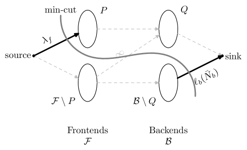
Figure 5: Illustration of the Third Type of Cut

B.2 Proof of Lemma 2

Lemma.

The optimal $\bm{N}^{*}$ to the fluid optimization problem (1) is unique.

Proof.

Suppose not. There exists $(\bm{x},\bm{N})$ and $(\bm{x}^{\prime},\bm{N}^{\prime})$ both optimal and $\bm{N}\neq\bm{N}^{\prime}$. Now consider $\tilde{\bm{x}}=({\bm{x}+\bm{x}^{\prime}})/{2}$, then for all $b\in\mathcal{B}$,

$$\tilde{N}_{b}=\ell^{-1}_{b}\left(\sum_{f\in\mathcal{F}(b)}\lambda_{f}\frac{x_{f,b}+x^{\prime}_{f,b}}{2}\right)<\frac{1}{2}\ell_{b}^{-1}\left(\sum_{f\in\mathcal{F}(b)}\lambda_{f}x_{f,b}\right)+\frac{1}{2}\ell_{b}^{-1}\left(\sum_{f\in\mathcal{F}(b)}\lambda_{f}x^{\prime}_{f,b}\right)=\frac{N_{b}+N^{\prime}_{b}}{2},$$

where the inequality follows as $\{\ell_{b}\}_{b\in\mathcal{B}}$ are strictly increasing and strongly concave by assumption, thus $\{\ell^{-1}_{b}\}_{b\in\mathcal{B}}$ are strictly increasing and strongly convex. Therefore, the objective value corresponding to $\tilde{\bm{x}},\tilde{\bm{N}}$ is even smaller than the optimal objective value, which is a contradiction.∎

B.3 Proof of Lemma 3

Lemma.

Let $(\bm{N},\bm{x})$ denote a feasible solution to the fluid optimization problem (1), then $(\bm{N},\bm{x})$ is optimal if and only if for each frontend $f\in\mathcal{F}$ there exists a constant $c_{f}$ such that for $b\in\mathcal{B}(f)$ we have $1/\ell_{b}^{\prime}(N_{b})\geq c_{f}$ with equality holding if $x_{f,b}>0$.

Proof.

We first argue the conditions in the statement are necessary. As the service rate function is strictly increasing by assumption, it is invertible so we can rewrite the optimization problem with $\bm{x}$ as the decision variables. Let $N_{b}(\bm{x})=\ell_{b}^{-1}\left(\sum_{f\in\mathcal{F}(b)}\lambda_{f}x_{f,b}\right)$. Pre-multiplying the flow balance constraint of frontend $f$ by $\lambda_{f}$, we obtain by using the method of Lagrange multipliers:

$$L(\bm{x},\bm{c},\bm{\alpha})=\sum_{b\in\mathcal{B}}N_{b}(\bm{x})+\sum_{f\in\mathcal{F}}c_{f}\lambda_{f}\left(1-\sum_{b\in\mathcal{B}(f)}x_{f,b}\right)+\sum_{(f,b)\in\mathcal{E}}\alpha_{f,b}x_{f,b}\,,$$

where $c_{f}$ are the Lagrange multiplier of the frontends flow balance constraint and $\alpha_{f,b}$ are the Lagrange multipliers of the non-negativity constraints.

The Karush–Kuhn–Tucker conditions are

$$\frac{\partial N_{b}(\bm{x})}{\partial x_{f,b}}-c_{f}\lambda_{f}-\alpha_{f,b}=0,\forall(f,b)\in\mathcal{E},$$

$$\sum_{b\in\mathcal{B}(f)}x_{f,b}=1,\forall f\in\mathcal{F},$$

$$\alpha_{f,b}x_{f,b}=0,\forall(f,b)\in\mathcal{E},$$

$$\alpha_{f,b}\geq 0,x_{f,b}\geq 0,\forall(f,b)\in\mathcal{E},$$

$$x_{f,b}=0,\forall(f,b)\not\in\mathcal{E}.$$

By the implicit function theorem, $\partial N_{b}(\bm{x})/\partial x_{f,b}=\lambda_{f}/\ell_{b}^{\prime}(N_{b})$. Therefore, for $x_{f,b}^{*}>0$ complementary slackness implies $\alpha_{f,b}=0$ and

$$\frac{\lambda_{f}}{\ell_{b}^{\prime}(N_{b}^{*})}=\lambda_{f}c_{f}\,.$$

For $(f,b)\in\mathcal{E}$ with $x_{f,b}^{*}=0$ we have $\alpha_{f,b}\geq 0$ and thus

$$\frac{\lambda_{f}}{\ell_{b}^{\prime}(N_{b}^{*})}\geq\lambda_{f}c_{f}.$$

The result follows by dividing both conditions by $\lambda_{f}>0$.

Sufficiency follows because the problem is convex since the feasible set is linear and $N_{b}(\bm{x})$ is convex. Therefore, the first-order conditions are sufficient for optimality. ∎

B.4 Proof of Theorem 1

Theorem.

Almost surely, the set of sub-sequential limits of $\{\bar{\bm{Y}}^{(c)}(\cdot)\}$ in $C([0,T],\mathbb{R}^{|\mathcal{B}|})$ as $c\to\infty$ is non-empty, and for every such limit point $\bm{y}(\cdot)$, there exists $\bm{x}_{f}(t)\in X_{f}(\bm{N}(t))$ for all $f\in\mathcal{F}$, $t\in[0,T]$ such that $\bm{y}(\cdot)$ satisfies

$$y_{b}(t)=y_{b}(0)+\int_{0}^{t}\left(\sum_{f\in\mathcal{F}(b)}\lambda_{f}x_{f,b}(\tau)-\ell_{b}(y_{b}(\tau))\right)\,d\tau\text{ for all }b\in\mathcal{B},t\in[0,T].$$

First Part

We have that $Y_{b}^{(c)}(n):=N_{b}^{(c)}(n)/c$ satisfies the following stochasic recursive inclusion

$$Y_{b}^{(c)}(n+1) =Y_{b}^{(c)}(n)+\frac{1}{c}\left(\sum_{f\in\mathcal{F}(b)}A_{f,b}^{(c)}(n)-D_{b}^{(c)}(n)\right)$$

$$=Y_{b}^{(c)}(n)+\frac{1}{c}\underbrace{\left(\sum_{f\in\mathcal{F}(b)}\lambda_{f}x^{(c)}_{f,b}(n)-\ell_{b}(Y_{b}^{(c)}(n))\right)}_{g^{(c)}_{b}(n)}$$

$$\quad\quad+\frac{1}{c}\underbrace{\left(\sum_{f\in\mathcal{F}(b)}A_{f,b}^{(c)}(n)-D_{b}^{(c)}(n)-\left(\sum_{f\in\mathcal{F}(b)}\lambda_{f}x^{(c)}_{f,b}(n)-\ell_{b}(Y_{b}^{(c)}(n))\right)\right)}_{\varepsilon_{b}^{(c)}(n+1)}$$

$$=Y_{b}^{(c)}(n)+\frac{1}{c}\left(g^{(c)}_{b}(n)+\varepsilon_{b}^{(c)}(n+1)\right).$$

We hereafter move the time step index $n$ to the subscript, i.e.,

$$\bm{Y}^{(c)}_{n+1}=\bm{Y}^{(c)}_{n}+\frac{1}{c}\left(\bm{g}^{(c)}_{n}+\bm{\varepsilon}^{(c)}_{n+1}\right),$$ (9)

where $\bm{\varepsilon}^{(c)}_{n+1}$ is the difference between a random variable and its mean, which can be viewed as the noise added to the system. Specifically, $\{\bm{\varepsilon}^{(c)}_{n}\}$ is a martingale difference sequence with respect to the past:

$$\mathbb{E}[\bm{\varepsilon}^{(c)}_{n+1}|\sigma(\bm{Y}^{(c)}_{m},\bm{\varepsilon}^{(c)}_{m},m\leq n)]=0\text{ a.s., }n\geq 0.$$

To prove the relative compactness of the linear interpolations $\{\bar{\bm{Y}}^{(c)}(\cdot)\}_{c\in\mathbb{N}}$, we show an equivalence between it and the following differential sequence, whose relative compactness is straight-forward.

Let’s define a continuous, piecewise constant $\bar{\bm{g}}^{(c)}(t)$, $t\in[0,T]$ where $\bar{\bm{g}}^{(c)}(n/c)=\bm{g}^{(c)}_{n}$, $n\geq 0$ and on each interval $t\in[n/c,(n+1)/c]$,

$$\bar{\bm{g}}^{(c)}(t)=\bm{g}^{(c)}_{n}.$$

Let $\bm{y}^{(c)}(\cdot)$ denote the integrals of the piecewise linear $\bar{\bm{g}}^{(c)}(\cdot)$ that start with $\bar{\bm{Y}}^{(c)}(0)$ at time 0, i.e.,

$${\bm{y}}^{(c)}(t)=\bm{y}^{(c)}(0)+\int_{0}^{t}\bar{\bm{g}}^{(c)}(t),\bm{y}^{(c)}(0)=\bar{\bm{Y}}^{(c)}(0).$$

Here process $\bm{y}^{(c)}(\cdot)$ is the compensator of the process $\bm{Y}^{(c)}(\cdot)$, i.e., the integral of the drift; and we will work with $\bm{y}^{(c)}(\cdot)$ as it allows us to work with the expected values. Using that $\sup_{n\leq\lceil Tc\rceil}\|\bm{g}^{(c)}_{n}\|<\infty$ a.s., we have that $\{\bm{y}^{(c)}(\cdot)\}_{c\in\mathbb{N}}$ is equicontinuous and pointwise bounded. By the Arzela-Ascoli Theorem, it is relatively compact in $C([0,T];\mathbb{R}^{|\mathcal{B}|})$. The following lemma allows us to pass the relative compactness to $\bm{Y}^{(c)}(\cdot)$.

Lemma 17.

For any $T>0$, let $\|\cdot\|$ denote Euclidean norm, we have

$$\lim_{c\to\infty}\sup_{t\in[0,T]}\|\bar{\bm{Y}}^{(c)}(t)-\bm{y}^{(c)}(t)\|=0,\text{ a.s..}$$

Proof.

Let’s fix a sample path and fix $t\in[0,T]$, let $[t]:=\max\{n/c:n/c\leq t,n\in\mathbb{N}\}$, then

$$\bm{y}^{(c)}(t) \stackrel{{\scriptstyle(a)}}{{=}}\bm{y}^{(c)}(0)+\int_{0}^{t}\bar{\bm{g}}^{(c)}(u)\,du$$

$$\stackrel{{\scriptstyle(b)}}{{=}}\bar{\bm{Y}}^{(c)}(0)+\int_{0}^{[t]}\bar{\bm{g}}^{(c)}(u)\,du+\int_{[t]}^{t}\bar{\bm{g}}^{(c)}(u)\,du$$

$$\stackrel{{\scriptstyle(c)}}{{=}}\bar{\bm{Y}}^{(c)}(0)+\sum_{k=0}^{[t]-1}\frac{1}{c}{\bm{g}}^{(c)}_{k}+\int_{[t]}^{t}\bar{\bm{g}}^{(c)}(u)\,du$$

$$\stackrel{{\scriptstyle(d)}}{{=}}\bar{\bm{Y}}^{(c)}([t])-\sum_{k=1}^{[t]}\frac{1}{c}\bm{\varepsilon}^{(c)}_{k}+\int_{[t]}^{t}\bar{\bm{g}}^{(c)}(u)\,du$$

$$\stackrel{{\scriptstyle(e)}}{{=}}\bar{\bm{Y}}^{(c)}(t)-\sum_{k=1}^{[t]}\frac{1}{c}\bm{\varepsilon}^{(c)}_{k}+\left(\bar{\bm{Y}}^{(c)}([t])+\int_{[t]}^{t}\bar{\bm{g}}^{(c)}(u)\,du-\bar{\bm{Y}}^{(c)}(t)\right),$$

where $(a)$ follows as $\bm{y}^{(c)}(\cdot)$ is the solution to the differential equation $\dot{\bm{y}}^{(c)}(t)=\bar{\bm{g}}^{(c)}(t)$; $(b)$ follows as $\bm{y}^{(c)}(0)=\bar{\bm{Y}}^{(c)}(0)$ by definition; $(c)$ follows as $\bar{\bm{g}}^{(c)}(t)=\bm{g}^{(c)}_{n},t\in[n/c,(n+1)/c]$ are piecewise constant in each interval; $(d)$ follows as $\bar{\bm{Y}}^{(c)}(0)=\bm{Y}^{(c)}_{0}$, $\bar{\bm{Y}}^{(c)}([t])=\bm{Y}^{(c)}_{[t]}$ and the stochastic recursion (9); $(e)$ follows by adding and subtracting $\bar{\bm{Y}}^{(c)}(t)$.

We proceed to bound the norm of the term in the bracket:

$$\left\|\bar{\bm{Y}}^{(c)}([t])+\int_{[t]}^{t}\bar{\bm{g}}^{(c)}(u)\,du-\bar{\bm{Y}}^{(c)}(t)\right\| \stackrel{{\scriptstyle(a)}}{{\leq}}\|\bar{\bm{Y}}^{(c)}([t])-\bar{\bm{Y}}^{(c)}(t)\|+\int_{[t]}^{t}\|\bar{\bm{g}}^{(c)}(u)\|\,du$$

$$\stackrel{{\scriptstyle(b)}}{{\leq}}\frac{1}{c}(\|\bm{\varepsilon}^{(c)}_{[t]+1}\|+2\|{\bm{g}}^{(c)}_{[t]}\|),$$

where $(a)$ follows the triangle inequality; $(b)$ follows from $\bar{\bm{Y}}^{(c)}([t])-\bar{\bm{Y}}^{(c)}(t)\leq([t]-t)({\bm{g}}^{(c)}_{[t]}+\bm{\varepsilon}^{(c)}_{[t]+1})$ and $[t]-t<1/c$, and $\int_{[t]}^{t}\|\bar{\bm{g}}^{(c)}(u)\|\,du=(t-[t])\|{\bm{g}}^{(c)}_{[t]}\|\leq\frac{1}{c}\|{\bm{g}}^{(c)}_{[t]}\|$.

By Lemma 18 and $\ell_{b}$ are bounded by assumption, we have

$$\lim_{c\to\infty}\frac{1}{c}\sup_{1\leq n\leq Tc}(\|\bm{\varepsilon}^{(c)}_{[t]}\|+2\|{\bm{g}}^{(c)}_{[t]}\|)=0.$$

Combining with Lemma 19, the result thus follows. ∎

Therefore, Lemma 17 implies that $\{\bar{\bm{Y}}^{(c)}(\cdot)\}_{c\in\mathbb{N}}$ is also relatively compact, otherwise this contradicts the compactness of $\{\bm{y}^{(c)}(\cdot)\}_{c\in\mathbb{N}}$.

Thus, there exists a subsequence such that

$$\bar{\bm{Y}}^{(c)}(\cdot)\to\bm{y}(\cdot)\text{ in }C([0,T];\mathbb{R}^{|\mathcal{B}|}).$$

As $\{\bar{\bm{g}}^{(c)}(\cdot)\}_{c\in\mathbb{N}}$ is a subset of $L_{2}([0,T],\mathbb{R}^{|\mathcal{B}|})$ with bounded norm, by the Banach-Alaoglu Theorem (Rudin, 1991) it is weakly relatively sequentially compact. Thus, the subsequence has a further subsubsequence such that

$$\bar{\bm{g}}^{(c)}(\cdot)\to\bm{g}(\cdot)\text{ weakly in }L^{2}([0,T];\mathbb{R}^{|\mathcal{B}|}).$$

Recall that

$$\bm{y}^{(c)}(t)=\bm{y}^{(c)}(0)+\int_{0}^{t}\bar{\bm{g}}^{(c)}(u)\,du,$$

taking $c\to\infty$ we have

$$\bm{y}(t)=\bm{y}(0)+\int_{0}^{t}\bm{g}(u)\,du.$$

We conclude by showing that $\bm{g}(u)\in H(\bm{y}(u))$ for $u\in[0,t]$.

By the Banach-Saks Theorem (Partington, 1977), as $\bar{\bm{g}}^{(c)}(\cdot)\to\bm{g}(\cdot)\text{ weakly in }L^{2}([0,T];\mathbb{R}^{|\mathcal{B}|})$, passing to a subsequence, which we denote by $\bar{g}^{(c)}(\cdot)$ to simplify notation,

$$\frac{1}{c}\sum_{i=1}^{c}\bar{\bm{g}}^{(i)}(\cdot)\to\bm{g}(\cdot)\text{ almost everywhere.}$$

Recall $[t]:=\max\{n/c:n/c\leq t,n\in\mathbb{N}\}$, we have $\bar{\bm{g}}^{(c)}(u)={\bm{g}}^{(c)}_{[u]}\in H(\bm{Y}^{(c)}_{[u]})$, and as $c\to\infty$, we have $\bm{Y}^{(c)}_{[u]}\to\bar{\bm{Y}}^{(c)}(u)$ and $\bar{\bm{Y}}^{(c)}(u)\to\bm{y}(u)$, thus

$$\bar{\bm{g}}^{(c)}(u)\to H(\bm{y}(u)).$$

Finally, as $H$ is upper semi-continuous with convex and compact values, we have for $u\in[0,t]$

$$\bm{g}(u)\in H(\bm{y}(u)).$$

Lemma 18.

Let $Z_{b}^{(c)}(n)=\sum_{f\in\mathcal{F}(b)}A_{f,b}^{(c)}(n)-D_{b}^{(c)}(n)$, for any $T>0$,

$$\lim_{c\to\infty}\sup_{1\leq n\leq Tc}\frac{1}{c}|Z_{b}^{(c)}(n)|=0\text{ a.s.. }$$

Proof.

For any $\epsilon>0$, let $2<q\leq 4$,

$$\mathbb{P}\left(\sup_{1\leq n\leq Tc}\frac{1}{c}|Z_{b}^{(c)}(n)|>\epsilon\right) \stackrel{{\scriptstyle(a)}}{{\leq}}\frac{\mathbb{E}\left[\sup_{1\leq n\leq Tc}|Z_{b}^{(c)}(n)|^{q}\right]}{c^{q}\epsilon^{q}}$$

$$\stackrel{{\scriptstyle(b)}}{{\leq}}\frac{\sum_{1\leq n\leq Tc}\mathbb{E}\left[|Z_{b}^{(c)}(n)|^{q}\right]}{c^{q}\epsilon^{q}}$$

$$\stackrel{{\scriptstyle(c)}}{{\leq}}\frac{TcK_{z}}{c^{q}\epsilon^{q}},$$

where $(a)$ follows Chebyshev’s inequality; $(b)$ follows as for any sequence $\{a_{n}\}$, we have $\sum_{n}|a_{n}|\geq\sup_{n}|a_{n}|$; $(c)$ follows by Minkowski’s Inequality and the definition of $Z_{b}^{(c)}(n)$:

$$\left(\mathbb{E}\left[|Z_{b}^{(c)}(n)|^{q}\right]\right)^{1/q}\leq\sum_{f\in\mathcal{F}(b)}\left(\mathbb{E}\left[|A_{f,b}^{(c)}(n)|^{q}\right]\right)^{1/q}+\left(\mathbb{E}\left[|D_{b}^{(c)}(n)|^{q}\right]\right)^{1/q}\leq K_{z}^{1/q},$$ (10)

here $K_{z}^{1/q}$ is a finite constant as $A_{f,b}^{(c)}(n)\leq\sum_{b\in\mathcal{B}(f)}A_{f,b}^{(c)}(n)$, where the right-hand-side of the inequality is a Poisson random variables with rate $\lambda_{f}<\infty$; and that $D_{b}^{(c)}(n)$ has finite fourth moment.

Therefore,

$$\sum_{c=1}^{\infty}\mathbb{P}\left(\sup_{1\leq n\leq Tc}\frac{1}{c}|Z_{b}^{(c)}(n)|>\epsilon\right)\leq\sum_{c=1}^{\infty}\frac{TK_{z}}{c^{q-1}\epsilon^{q}}<\infty.$$

By Borel-Cantelli lemma, as $\epsilon>0$ was arbitrary, the result follows. ∎

Lemma 19.

For any $T>0$,

$$\lim_{c\to\infty}\sup_{1\leq n\leq Tc}\frac{1}{c}\sum_{k=1}^{n}\bm{\varepsilon}^{(c)}_{k}=0\text{ a.s..}$$

Proof.

As $\{\bm{\varepsilon}^{(c)}_{k}\}$ is martingale difference, we have $M_{n}^{(c)}=\sum_{k=1}^{n}\bm{\varepsilon}^{(c)}_{k}$ is a martingale with respect to $\{\sigma(\bm{\varepsilon}^{(c)}_{1},\ldots,\bm{\varepsilon}^{(c)}_{n-1})\}$.

We then have

$$\mathbb{E}\left[(M_{n}^{c})^{4}\right] \stackrel{{\scriptstyle(a)}}{{\leq}}K_{4}\mathbb{E}\left[\left(\sum_{k=1}^{n}(\bm{\varepsilon}^{(c)}_{k})^{2}\right)^{2}\right]$$

$$=K_{4}\mathbb{E}\left[\sum_{1\leq i,j\leq n}(\bm{\varepsilon}^{(c)}_{i})^{2}(\bm{\varepsilon}^{(c)}_{j})^{2}\right]$$

$$\stackrel{{\scriptstyle(b)}}{{=}}K_{4}\sum_{1\leq i,j\leq n}\mathbb{E}\left[(\bm{\varepsilon}^{(c)}_{i})^{2}(\bm{\varepsilon}^{(c)}_{j})^{2}\right]$$

$$\stackrel{{\scriptstyle(c)}}{{\leq}}K_{4}\sum_{1\leq i,j\leq n}\sqrt{\mathbb{E}[(\bm{\varepsilon}^{(c)}_{i})^{4}]}\sqrt{\mathbb{E}[(\bm{\varepsilon}^{(c)}_{j})^{4}]}$$

$$\stackrel{{\scriptstyle(d)}}{{\leq}}K_{m}n^{2}.$$

where $(a)$ follows from Burkholder’s Inequality (Burkholder (1966) Theorem 9) with $K_{4}>0$ being a constant; $(b)$ follows from linearity of expectation; $(c)$ follows from Cauchy–Schwarz inequality; $(d)$ follows from (10) where we show $\mathbb{E}[(\bm{\varepsilon}^{(c)}_{i})^{4}]<\infty$, $K_{m}>0$ is a constant.

Therefore, by Doob’s Maximal inequality,

$$\mathbb{P}\left(\sup_{1\leq n\leq Tc}|M_{n}^{(c)}|\geq c\epsilon\right)\leq\frac{\mathbb{E}[\max\{(M_{\lceil Tc\rceil}^{c})^{4},0\}]}{(c\epsilon)^{4}}=\frac{\mathbb{E}[(M_{\lceil Tc\rceil}^{c})^{4}]}{(c\epsilon)^{4}}\leq\frac{K_{m}T^{2}}{\epsilon^{4}c^{2}},$$

which implies

$$\sum_{c=1}^{\infty}\mathbb{P}\left(\sup_{1\leq n\leq Tc}|M_{n}^{(c)}|\geq c\epsilon\right)<\infty.$$

By Borel-Cantelli Lemma, as $\epsilon>0$ was arbitrary, the result follows. ∎

Theorem 4 (Theorem 9 Burkholder (1966)).

Let $1<p<\infty$. There are positive real numbers $k_{p},K_{p}$ such that if $\{M_{n}\}$ is a martingale then

$$k_{p}\mathbb{E}[S_{n}^{p}]\leq\mathbb{E}[|M_{n}|^{p}]\leq K_{p}\mathbb{E}[S_{n}^{p}],$$

where $S_{n}=\sqrt{\sum_{k=1}^{n}(M_{k}-M_{k-1})^{2}}$, $M_{0}=0$.

Appendix C Differential Inclusion

Definition 7 (Definition 1.4.1 Aubin and Frankowska (1990)).

A set-valued map $H:\mathcal{N}\mapsto\mathcal{V}$ is called upper semi-continuous at $\bm{N}_{0}\in\mathcal{N}$ if for any open set $M$ containing $H(\bm{N}_{0})$ there exists a neighborhood $\Omega$ of $\bm{N}_{0}$ such that $H(\Omega)\subset M$. A set-valued map $H$ is said to be upper semi-continuous if it is so at every point $\bm{N}_{0}\in\mathcal{N}$.

Definition 8 (Definition 2.2.1 Kunze (2000)).

Let $I\subseteq\mathbb{R}$ be an interval with $0\in I$, $\mathcal{N}\subseteq\mathbb{R}^{n},\bm{N}_{0}\in\mathcal{N}$, and $H:\mathcal{N}\mapsto\mathcal{V}$ a multi-valued mapping. A function $\bm{N}$ such that

• $\bm{N}:I\mapsto\mathcal{N}$ is absolutely continuous on $I$,

• $\bm{N}(0)=\bm{N}_{0}$, and

• $\dot{\bm{N}}(t)\in H(\bm{N}(t))$ for almost everywhere $t\in I$

is called a solution of the differential inclusion $\dot{\bm{N}}\in H(\bm{N})$ a.e., $\bm{N}(0)=\bm{N}_{0}$.

Theorem 5 (Theorem 4, Chapter 2, Section 1 Aubin and Cellina (1984)).

Let $F$ be an upper semi-continuous map from $\mathcal{N}\mapsto\mathcal{N}$ with non-empty closed convex values. We suppose that $\pi_{H(\bm{N})}(0)$ (the element in $H(\bm{N})$ with the minimal norm) remains in a compact subset of $\mathcal{N}$. For any $\bm{N}_{0}\in\mathcal{N}$, there exists an absolutely continuous function defined on $[0,\infty)$,a solution to $\dot{\bm{N}}(t)\in H(\bm{N}(t)),\bm{N}(0)=\bm{N}_{0}$.

C.1 Proof of Existence of Solution to the Differential Inclusion (3)

Lemma 20 (Existence of Solution).

For any $\bm{N}_{0}\geq\bm{0}$, there exists an absolutely continuous function defined on $[0,\infty)$, a solution to the differential inclusion (3) with $\bm{N}(0)=\bm{N}_{0}$.

Proof.

First note the feasible set of the optimization problem (2) is nonempty, compact valued, and continuous. The objective function is also a continuous function by assumption. Then by Berge’s Maximum Theorem, the optimal flow assignment correspondence $X_{f}(\cdot)$ is nonempty, compact valued, and upper semi-continuous.

Recall

$$H(\bm{N}):=\left\{(v_{1},\ldots,v_{|\mathcal{B}|}):v_{b}=\sum_{f\in\mathcal{F}(b)}\lambda_{f}x_{f,b}(t)-\ell_{b}(N_{b}(t)),\bm{x}_{f}\in X_{f}(\bm{N}),\forall f\in\mathcal{F},b\in\mathcal{B}\right\}$$ (11)

denote the right-hand-side of the differential inclusion, i.e., $\dot{\bm{N}}(t)\in H(\bm{N}(t))$. We proceed to show that $H(\cdot)$ is upper semi-continuous with closed convex values, then as the service rate functions are bounded, by Theorem 4, Chapter 2, Section 1 in Aubin and Cellina (1984), the existence of global solution (i.e., defined on $[0,\infty)$ follows.

The closed convex part is straightforward. Fix any $\bm{N}_{0}\geq\bm{0}$, for any open set $M$ such that $H(\bm{N})\subseteq M$, there must exists open sets $\{X_{f}\}_{f\in\mathcal{F}}$ such that $X_{f}(\bm{N}_{0})\subseteq X_{f}$ and

$$\left\{(v_{1},\ldots,v_{|\mathcal{B}|}):v_{b}=\sum_{f\in\mathcal{F}(b)}\lambda_{f}x_{f,b}(t)-\ell_{b}(N_{b}(t)),\bm{x}_{f}\in X_{f},\forall f\in\mathcal{F},b\in\mathcal{B}\right\}\subseteq M.$$

As $X_{f}(\cdot)$ is upper semi-continuous for all $f\in\mathcal{F}$, for any open set $X_{f}$ such that $X_{f}(\bm{N}_{0})\subseteq X_{f}$, there exists a neighborhood $\Omega_{f}$ of $\bm{N}_{0}$ such that for all $X_{f}(\Omega_{f})\subseteq X_{f}$. Therefore, let $\Omega=\cap_{f\in\mathcal{F}}\Omega_{f}$, we have for any $N^{\prime}\in\Omega$, $H(\bm{N}^{\prime})\subseteq M$. By definition, this implies that $H(\cdot)$ is upper semi-continuous. ∎

C.2 Proof of Lemma 4

Lemma.

The dynamic system (3) has a unique equilibrium point $\bm{N}^{eq}$, which is optimal for the fluid optimization problem (1).

Proof.

At an equilibrium point $\bm{N}^{eq}$, we must have the temporal derivatives equal zero, i.e., $\bm{0}\in H(\bm{N}^{eq})$. Therefore, there exists $\bm{x}_{f}\in X_{f}(\bm{N}^{eq})$ for all $f\in\mathcal{F}$ such that

$$\sum_{f\in\mathcal{F}(b)}\lambda_{f}x_{f,b}=\ell_{b}(N_{b}^{eq}),\forall b\in\mathcal{B}.$$

Therefore, $(\bm{N}^{eq},\bm{x})$ is a feasible solution to the optimization problem (1). Moreover, by definition of $X_{f}(\bm{N})$, if $x_{f,b}>0$, $\ell^{\prime}_{b}(N_{b})=\max_{j\in\mathcal{B}(f)}\ell^{\prime}_{j}(N_{j})$. Then by Lemma 3, $\bm{N}^{eq}$ satisfy the first-order conditions, which we prove is also sufficient, thus $\bm{N}^{eq}$ is optimal for (1). The uniqueness follows as the fluid optimization problem has a unique solution (Lemma 2) and every equilibrium point is optimal. ∎

Appendix D Stability Analyses

D.1 Proof of Lemma 5

Lemma.

The function $V(\bm{N},\bm{x})=\sum_{b\in\mathcal{B}}|\sum_{f\in\mathcal{F}(b)}\lambda_{f}x_{f,b}-\ell_{b}(N_{b})|$ is positive definite, i.e., $V(\bm{N},\bm{x})\geq 0$ for all $\bm{N},\bm{x}$ and for all $\bm{x}_{f}\in X_{f}(\bm{N})$ we have

$$V(\bm{N},\bm{x})=0\text{ if and only if }(\bm{N},\bm{x})=(\bm{N}^{*},\bm{x}^{*}),$$

where $\bm{x}^{*}$ satisfies $\sum_{f\in\mathcal{F}(b)}\lambda_{f}x_{f,b}^{*}-\ell_{b}(N_{b}^{*})=0$ for all $b\in\mathcal{B}$.

Proof.

If $(\bm{N},\bm{x})=(\bm{N}^{*},\bm{x}^{*})$, then $V(\bm{N},\bm{x})=\sum_{b\in\mathcal{B}}|\sum_{f\in\mathcal{F}(b)}\lambda_{f}x_{f,b}^{*}-\ell_{b}(N_{b}^{*})|=0$ by the definition of $\bm{x}^{*}$.

If $V(\bm{N},\bm{x})=0$, then we must have $\sum_{f\in\mathcal{F}(b)}\lambda_{f}x_{f,b}-\ell_{b}(N_{b})=0$ for all $b\in\mathcal{B}$. Meanwhile, as $\bm{x}_{f}\in X_{f}(\bm{N})$, this implies $\sum_{b\in\mathcal{B}(f)}x_{f,b}=1$ and $\bm{x}_{f}\geq\bm{0}$ for all $f\in\mathcal{F}$. Therefore, $\bm{N}$ is a feasible solution to the optimization problem (1).

Moreover, for any $f\in\mathcal{F}$, as $\bm{x}_{f}\in X_{f}(\bm{N})$

$$\ell_{b_{1}}^{\prime}(N_{b_{1}})=\ell_{b_{2}}^{\prime}(N_{b_{2}})\text{ for }b_{1},b_{2}\in\{b\in\mathcal{B}(f):x_{f,b}>0\},$$

Therefore, by Lemma 3, $\bm{N}=\bm{N}^{*}$, which implies $\bm{x}=\bm{x}^{*}$.∎

D.2 TierGraphs

Proof of Lemma 6

Lemma.

For two tiers $(F_{i},B_{i}),(F_{j},B_{j})$ with $F_{i},F_{j}\subseteq\mathcal{F},B_{i},B_{j}\subseteq\mathcal{B}$ at $\bm{N}$, let vertex $v_{i}$ and vertex $v_{j}$ denote their corresponding vertices in the TierGraph $\mathcal{T}(\bm{N})$. If $v_{i}\to v_{j}$, then $\ell_{B_{i}}^{\prime}(\bm{N})>\ell_{B_{j}}^{\prime}(\bm{N})$.

Proof.

By Definition 4, $v_{i}\to v_{j}$ implies there exists $f\in F_{i}\cap B_{j}$ such that $(f,b)\in E$. Therefore, by Definition 3, $b\notin S_{f}(\bm{N})$, i.e., $\ell_{B_{i}}^{\prime}(\bm{N})>\ell_{B_{j}}^{\prime}(\bm{N})$.∎

Proof of Corollary 1

Corollary.

For two tiers $(F_{i},B_{i}),(F_{j},B_{j})$ with $F_{i},F_{j}\subseteq\mathcal{F},B_{i},B_{j}\subseteq\mathcal{B}$ at $\bm{N}$, if $(F_{i},B_{i})\prec(F_{j},B_{j})$, then $\ell_{B_{i}}^{\prime}(\bm{N})>\ell_{B_{j}}^{\prime}(\bm{N})$.

Proof.

By Definition 4, $(F_{i},B_{i})\prec(F_{j},B_{j})$ implies that in the TierGraph $\mathcal{T}(\bm{N})$, vertex $v_{i}$ can reach vertex $v_{j}$, i.e., there exists a sequence of vertices $v_{a_{1}},v_{a_{2}},\ldots,v_{a_{k}}$ such that

$$v_{i}\to v_{a_{1}}\to v_{a_{2}}\to\cdots\to v_{a_{k}}\to v_{j}$$

in the TierGraph $\mathcal{T}(\bm{N})$. By Lemma 6, we then have

$$\ell_{B_{i}}^{\prime}(\bm{N})>\ell_{B_{a_{1}}}^{\prime}(\bm{N})>\ell_{B_{a_{2}}}^{\prime}(\bm{N})>\cdots>\ell_{B_{a_{k}}}^{\prime}(\bm{N})>\ell_{B_{j}}^{\prime}(\bm{N}).\qed$$

Proof of Corollary 2

Corollary.

The TierGraph $\mathcal{T}(\bm{N})$ is a directed acyclic graph.

Proof.

Suppose not, i.e., there exists a sequence of vertices such that $v_{1}\to v_{2}\to\cdots\to v_{m}\to v_{1}$ in the TierGraph $\mathcal{T}(\bm{N})$. Then by Corollary 1, we have

$$\ell_{B_{1}}^{\prime}(\bm{N})>\ell_{B_{2}}^{\prime}(\bm{N})>\cdots>\ell_{B_{m}}^{\prime}(\bm{N})>\ell_{B_{1}}^{\prime}(\bm{N}),$$

which is a contradiction.∎

D.3 Proof of Lemma 7

Lemma.

If there exists $t_{1}<t_{2}$ and $F\subseteq\mathcal{F},B\subseteq\mathcal{B}$ such that $(F,B)$ is a tier at $\bm{N}(t)$ for $t\in[t_{1},t_{2}]$, then for any $b_{1},b_{2}\in B$, $\frac{d}{dt}N_{b_{1}}(t)\cdot\frac{d}{dt}N_{b_{2}}(t)\geq 0$ for $t\in[t_{1},t_{2}]$.

Proof.

As $(F,B)$ is a tier at $\bm{N}(t)$ for $t\in[t_{1},t_{2}]$, for any $b_{1},b_{2}\in B$, we have

$$\ell_{b_{1}}^{\prime}(N_{b_{1}}(t))=\ell_{b_{2}}^{\prime}(N_{b_{2}}(t)),\forall t\in[t_{1},t_{2}],$$

which implies by taking derivatives with respect to $t$,

$$\frac{d}{dt}\ell_{b_{1}}^{\prime}(N_{b_{1}}(t))=\frac{d}{dt}\ell_{b_{2}}^{\prime}(N_{b_{2}}(t)),\forall t\in[t_{1},t_{2}],$$

or equivalently,

$$\ell_{b_{1}}^{\prime\prime}(N_{b_{1}}(t))\frac{d}{dt}N_{b_{1}}(t)=\ell_{b_{2}}^{\prime\prime}(N_{b_{2}}(t))\frac{d}{dt}N_{b_{2}}(t),\forall t\in[t_{1},t_{2}].$$

Note that $\ell_{b}^{\prime\prime}(N_{b})<0$ for all $N_{b}\geq 0$ by assumption, the result thus follows.∎

D.4 Proof of Lemma 8

Lemma.

If there exists $t_{1}<t_{2}$ and $F\subseteq\mathcal{F},B\subseteq\mathcal{B}$ such that for $t\in[t_{1},t_{2}]$,

• $(F,B)$ is a tier at $\bm{N}(t)$,

• $\sum_{f\in F}\lambda_{f}-\sum_{b\in B}\ell_{b}(N_{b}(t))\geq 0$.

Then for $t\in[t_{1},t_{2}]$, the following holds:

• $N_{b}(t)$ is increasing in $t$ for all $b\in B$,

• for any subset of backends $Q\subseteq B$,

  $$\sum_{f\in F\cap(\cup_{b\in Q}\mathcal{F}(b))}\lambda_{f}\geq\sum_{b\in Q}\ell_{b}(N_{b}(t)).$$

Proof.

We first show $N_{b}(t)$ is increasing for all $b\in B,t\in[t_{1},t_{2}]$.

$$\sum_{b\in B}\dot{N}_{b}(t) \stackrel{{\scriptstyle(a)}}{{=}}\sum_{b\in B}\left(\sum_{f\in F\cap\mathcal{F}(b)}\lambda_{f}x_{f,b}(t)-\ell_{b}(N_{b}(t))\right)$$

$$=\sum_{f\in F}\lambda_{f}\sum_{b\in B\cap\mathcal{B}(f)}x_{f,b}-\sum_{b\in B}\ell_{b}(N_{b}(t))$$

$$\stackrel{{\scriptstyle(b)}}{{=}}\sum_{f\in F}\lambda_{f}-\sum_{b\in B}\ell_{b}(N_{b}(t))\stackrel{{\scriptstyle(c)}}{{\geq}}0,$$ (12)

where $(a)$ follows from the definition of the differential inclusion (3); $(b)$ follows from $\sum_{b\in B\cap\mathcal{B}(f)}x_{f,b}(t)=1$ for all $f\in F$; $(c)$ follows from the assumption.

Combined with Lemma 7, i.e., the change in workloads at the backends in the same tier must have the same direction, we have $\dot{N}_{b}(t)\geq 0$ for all $b\in B$.

Therefore, this means for $t\in[t_{1},t_{2}]$, there must exist $\{x_{f,b}(t)\}_{f\in F\cap B}$ such that

$$\frac{d}{dt}N_{b}(t)=\sum_{f\in F\cap\mathcal{F}(b)}\lambda_{f}x_{f,b}(t)-\ell_{b}(N_{b}(t))\geq 0$$ (13)

$$0\leq x_{f,b}\leq 1,\forall f_{1}\in F\cap B,$$

$$\sum_{b\in B\cap\mathcal{B}(f)}x_{f,b}=1,\forall f\in F,$$

where the last two constraints follow from the definition of the differential inclusion (3).

Therefore, for any subset of backends $Q\subseteq B$,

$$\sum_{b\in Q}\ell_{b}(N_{b}(t))\stackrel{{\scriptstyle(d)}}{{\leq}}\sum_{b\in Q}\sum_{f\in F\cap\mathcal{F}(b)}\lambda_{f}x_{f,b}(t)=\sum_{f\in F\cap(\cup_{b\in Q}\mathcal{F}(b))}\lambda_{f}x_{f,b}(t)\stackrel{{\scriptstyle(e)}}{{\leq}}\sum_{f\in F\cap(\cup_{b\in Q}\mathcal{F}(b))}\lambda_{f}.$$

where $(d)$ follows inequality (13); $(e)$ holds as $x_{f,b}(t)\leq 1$.∎

D.5 Proof of Lemma 9

Lemma.

If there exists $t_{1}<t_{2}$ and $F\subseteq\mathcal{F},B\subseteq\mathcal{B}$ such that

• $(F,B)$ is a tier at $\bm{N}(t),t\in[t_{1},t_{2}]$,

• $\sum_{f\in F}\lambda_{f}-\sum_{b\in B}\ell_{b}(N_{b}(t))\leq 0$.

Then for $t\in[t_{1},t_{2}]$, the following holds:

• $N_{b}(t)$ is decreasing in $t$ for all $b\in B$,

• for any subset of frontends $P\subseteq F$,

  $$\sum_{f\in P}\lambda_{f}\leq\sum_{b\in B\cap(\cup_{f\in P}\mathcal{B}(f))}\ell_{b}(N_{b}(t)).$$

Proof.

Similar to the proof for Lemma 8, we can show that $N_{b}(\tau_{1})\leq N_{b}(\tau_{2})$ for any $\tau_{1}\leq\tau_{2}\in[t_{1},t_{2}]$, for all $b\in B$. Therefore, by definition of differential inclusion, there must exist $\{x_{f,b}(t)\}_{f\in F\cap B}$ such that

$$\frac{d}{dt}N_{b}(t)=\sum_{f\in F\cap\mathcal{F}(b)}\lambda_{f}x_{f,b}(t)-\ell_{b}(N_{b}(t))\leq 0,$$ (14)

$$0\leq x_{f,b}\leq 1,\forall f_{1}\in F\cap B,$$

$$\sum_{b\in B\cap\mathcal{B}(f)}x_{f,b}=1,\forall f\in F.$$ (15)

Therefore, for any subset of frontends $P\subseteq F$,

$$\sum_{f\in P}\lambda_{f} \stackrel{{\scriptstyle(a)}}{{=}}\sum_{f\in P}\lambda_{f}\sum_{b\in B\cap\mathcal{B}(f)}x_{f,b}(t)$$

$$=\sum_{b\in B\cap(\cup_{f\in P}\mathcal{B}(f))}\sum_{f\in P\cap\mathcal{F}(b)}\lambda_{f}x_{f,b}(t)$$

$$\stackrel{{\scriptstyle(b)}}{{\leq}}\sum_{b\in B\cap(\cup_{f\in P}\mathcal{B}(f))}\sum_{f\in F\cap\mathcal{F}(b)}\lambda_{f}x_{f,b}(t)$$

$$\stackrel{{\scriptstyle(c)}}{{\leq}}\sum_{b\in B\cap(\cup_{f\in P}\mathcal{B}(f))}\ell_{b}(N_{b}(t)),$$

where $(a)$ follows equality (15); $(b)$ holds as $P\subseteq F$; $(c)$ follows inequality (14).∎

D.6 Proof of Corollary 4

When the tier structure remains unchanged, the total flow imbalance never flips sign from positive to negative or vice versa. This is because flow imbalance drives workloads towards equilibrium, and when the flow is balanced, i.e., jobs arrive at the same rate as jobs depart, the workloads stabilize, and the total flow imbalance remains at zero. This observation is formalized in the following corollary.

Corollary 4.

If there exists $t_{1}<t_{2}$ and $F\subseteq\mathcal{F},B\subseteq\mathcal{B}$ such that for $t\in[t_{1},t_{2}]$, $(F,B)$ is a tier at $\bm{N}(t)$, then for $\tau_{1},\tau_{2}\in[t_{1},t_{2}]$,

$$\left(\sum_{f\in F}\lambda_{f}-\sum_{b\in B}\ell_{b}(N_{b}(\tau_{1}))\right)\cdot\left(\sum_{f\in F}\lambda_{f}-\sum_{b\in B}\ell_{b}(N_{b}(\tau_{2}))\right)\geq 0.$$

Proof.

By continuity of $\ell_{b}(N_{b}))$, the flow imbalance is also continuous in time. If there exists $t_{1}<\tau<t_{2}$ such that $\sum_{f\in F}\lambda_{f}-\sum_{b\in B}\ell_{b}(N_{b}(\tau))=0$, i.e., the total flow is balanced, then by Lemma 8, we have $\frac{d}{dt}N_{b}(t)|_{t=\tau}\geq 0$ for all $b\in B$; and by Lemma 9, we have $\frac{d}{dt}N_{b}(t)|_{t=\tau}\leq 0$ for all $b\in B$. Therefore, we must have $\frac{d}{dt}N_{b}(t)|_{t=\tau}=0$ for all $b\in B$. This implies $\sum_{f\in F}\lambda_{f}-\sum_{b\in B}\ell_{b}(N_{b}(t))=0$ for $t\in[\tau,t_{2}]$. ∎

D.7 Proof of Corollary 3

Corollary.

If there exists $F_{1},\ldots,F_{k}\subseteq\mathcal{F},B_{1},\ldots,B_{k}\subseteq\mathcal{B}$ such that

• $(F_{1},B_{1}),\ldots,(F_{k},B_{k})$ are tiers at $\bm{N}$,

• $\mathcal{F}=F_{1}\cup\cdots\cup F_{k}$ and $\mathcal{B}=B_{1}\cup\cdots\cup B_{k}$,

• $\sum_{f\in F_{i}}\lambda_{f}=\sum_{b\in B_{i}}\ell_{b}(N_{b})$ for all $i\in[k]$.

Then we must have $\bm{N}=\bm{N}^{*}$.

Proof.

The conditions imply that for all $f\in\mathcal{F}$ there exists $\bm{x}_{f}\in X_{f}(\bm{N})$ such that

$$\sum_{b\in\mathcal{B}}\left|\sum_{f\in\mathcal{F}(b)}\lambda_{f}x_{f,b}-\ell_{b}(N_{b})\right|=0.$$

Therefore, by Lemma 5, we must have $\bm{N}=\bm{N}^{*}$.∎

D.8 Proof of Lemma 10

Lemma.

If there exists $t_{1}<t_{2}$ and $F\subseteq\mathcal{F},B\subseteq\mathcal{B}$ such that for $t\in[t_{1},t_{2}]$, $(F,B)$ is a tier at $\bm{N}(t)$. Then, the total absolute drifts for the backends in $B$ satisfy

$$V_{B}(\bm{N}(t),\bm{x}(t))=\left|\sum_{f\in F}\lambda_{f}-\sum_{b\in B}\ell_{b}(N_{b}(t))\right|,$$

and $V_{B}(\bm{N}(t),\bm{x}(t))$ is non-increasing in $[t_{1},t_{2}]$.

Proof.

The total drift for the backends in $B$ is

$$V_{B}(\bm{N}(t),\bm{x}(t)) =\sum_{b\in B}\left|\sum_{f\in\mathcal{F}(b)}\lambda_{f}x_{f,b}(t)-\ell_{b}(N_{b}(t))\right|$$

$$\stackrel{{\scriptstyle(a)}}{{=}}\sum_{b\in B}\left|\sum_{f\in F\cap\mathcal{F}(b)}\lambda_{f}x_{f,b}(t)-\ell_{b}(N_{b}(t))\right|$$

$$\stackrel{{\scriptstyle(b)}}{{=}}\left|\sum_{b\in B}\sum_{f\in F\cap\mathcal{F}(b)}\lambda_{f}x_{f,b}(t)-\sum_{b\in B}\ell_{b}(N_{b}(t))\right|$$

$$=\left|\sum_{f\in F}\lambda_{f}\sum_{b\in B\cap\mathcal{B}(f)}x_{f,b}(t)-\sum_{b\in B}\ell_{b}(N_{b}(t))\right|$$

$$\stackrel{{\scriptstyle(c)}}{{=}}\left|\sum_{f\in F}\lambda_{f}-\sum_{b\in B}\ell_{b}(N_{b}(t))\right|,$$

where $(a)$ follows as $(F,B)$ is a tier, thus $x_{f,b}(t)=0$ for $b\in B\cap\mathcal{F}(b)\setminus F$; $(b)$ follows from Lemma 7 because flow balance for backends in a tier have the same sign; $(c)$ follows as $\sum_{b\in B\cap\mathcal{B}(f)}x_{f,b}(t)=1$ by flow balance at the frontends.

We conclude the proof by showing that $V_{B}(\bm{N}(t),\bm{x}(t))$ is decreasing in $[t_{1},t_{2}]$. If $\sum_{f\in F}\lambda_{f}\geq\sum_{b\in B}\ell_{b}(N_{b}(t_{1}))$. Then by Corollary 4, we have $\sum_{f\in F}\lambda_{f}\geq\sum_{b\in B}\ell_{b}(N_{b}(t))$ for $t\in[t_{1},t_{2}]$. Therefore, for $t\in[t_{1},t_{2}]$,

$$\frac{d}{dt}V_{B}(\bm{N}(t),\bm{x}(t)) =\frac{d}{dt}\left(\sum_{f\in F}\lambda_{f}-\sum_{b\in B}\ell_{b}(N_{b}(t))\right)$$

$$=-\sum_{b\in B}\ell^{\prime}_{b}(N_{b}(t))\frac{d}{dt}N_{b}(t)$$

$$\stackrel{{\scriptstyle(a)}}{{=}}-\ell_{B}^{\prime}(\bm{N}(t))\sum_{b\in B}\frac{d}{dt}N_{b}(t)$$

$$\stackrel{{\scriptstyle(b)}}{{=}}-\ell_{B}^{\prime}(\bm{N}(t))\left(\sum_{f\in F}\lambda_{f}-\sum_{b\in B}\ell_{b}(N_{b}(t))\right)$$

$$\stackrel{{\scriptstyle(c)}}{{\leq}}0.$$ (16)

where $(a)$ follows as all backends in a tier share the same gradient value and $\ell_{B}^{\prime}(\bm{N}(t))$ is used to denote this shared gradient value of this tier; $(b)$ follows (12); $(c)$ follows as $\ell_{b}^{\prime}(N_{b})>0$ by assumption and $\sum_{f\in F}\lambda_{f}\geq\sum_{b\in B}\ell_{b}(N_{b}(t))$ for $t\in[t_{1},t_{2}]$.

Similarly, if the tier has negative flow imbalance, for $t\in[t_{1},t_{2}]$,

$$\frac{d}{dt}V_{B}(\bm{N}(t),\bm{x}(t)) =\frac{d}{dt}\left(\sum_{b\in B}\ell_{b}(N_{b}(t))-\sum_{f\in F}\lambda_{f}\right)$$

$$=\sum_{b\in B}\ell^{\prime}_{b}(N_{b}(t))\frac{d}{dt}N_{b}(t)$$

$$\stackrel{{\scriptstyle(a)}}{{=}}\ell_{B}^{\prime}(\bm{N}(t))\sum_{b\in B}\frac{d}{dt}N_{b}(t)$$

$$\stackrel{{\scriptstyle(b)}}{{=}}\ell_{B}^{\prime}(\bm{N}(t))\left(\sum_{f\in F}\lambda_{f}-\sum_{b\in B}\ell_{b}(N_{b}(t))\right)$$

$$=-\ell_{B}^{\prime}(\bm{N}(t))\left(\sum_{b\in B}\ell_{b}(N_{b}(t))-\sum_{f\in F}\lambda_{f}\right)$$

$$\stackrel{{\scriptstyle(c)}}{{\leq}}0.$$ (17)

where $(a)$ follows as all backends in a tier share the same gradient value; $(b)$ follows (12); $(c)$ follows as $\ell_{b}^{\prime}(N_{b})>0$ by assumption and $\sum_{f\in F}\lambda_{f}\leq\sum_{b\in B}\ell_{b}(N_{b}(t))$ for $t\in[t_{1},t_{2}]$. ∎

D.9 Proof of Lemma 11

Lemma.

If there exists $t_{1}<\tau<t_{2}$ and $F\subseteq\mathcal{F},B\subseteq\mathcal{B}$ such that

• $(F,B)$ is a tier at $\bm{N}(t),t\in[t_{1},\tau)$,

• $(F,B)$ splits into ${\hat{k}}>1$ tiers $(\hat{F}_{1},\hat{B}_{1}),\ldots,(\hat{F}_{\hat{k}},\hat{B}_{\hat{k}})$ at $\bm{N}(t),t\in(\tau,t_{2}]$,

• $F=\hat{F}_{1}\cup\cdots\cup\hat{F}_{\hat{k}}$ and $B=\hat{B}_{1}\cup\cdots\cup\hat{B}_{\hat{k}}$,

Then the total absolute drifts for the backends in $B$ satisfy

$$V_{B}(\bm{N}(t),\bm{x}(t))=\left|\sum_{f\in F}\lambda_{f}-\sum_{b\in B}\ell_{b}(N_{b}(t))\right|,$$

and $V_{B}(\bm{N}(t),\bm{x}(t))$ is non-increasing in $[t_{1},t_{2}]$.

Proof.

First by Lemma 10, $V_{B}(\bm{N}(t),\bm{x}(t))=\left|\sum_{f\in F}\lambda_{f}-\sum_{b\in B}\ell_{b}(N_{b}(t))\right|$ for $t\in[t_{1},\tau)$. We proceed to show that this holds for $t\in(\tau,t_{2}]$.

• Suppose $\sum_{f\in F}\lambda_{f}-\sum_{b\in B}\ell_{b}(N_{b}(t))\geq 0$ for $t\in[t_{1},\tau)$, which we refer to as the tier having positive flow imbalance. We proceed to show that all tiers $(\hat{F}_{1},\hat{B}_{1}),\ldots,(\hat{F}_{\hat{k}},\hat{B}_{\hat{k}})$ also have positive flow imbalance for $t\in(\tau,t_{2}]$.

  Without loss of generality, let $\mathcal{T}(\bm{N}(t))$ denote the TierGraph that is restricted to tiers $(\hat{F}_{1},\hat{B}_{1}),\ldots,(\hat{F}_{\hat{k}},\hat{B}_{\hat{k}})$ for $t\in(\tau,t_{2}]$.

  • If $(\hat{F}_{i},\hat{B}_{i})$ corresponds to a source vertex in the TierGraph $\mathcal{T}(\bm{N}(t))$, then

    $$\sum_{b\in\hat{B}_{i}}\ell_{b}(N_{b}(\tau))\stackrel{{\scriptstyle(a)}}{{=}}\sum_{b\in\hat{B}_{i}}\ell_{b}(N_{b}(\tau^{-}))\stackrel{{\scriptstyle(b)}}{{\leq}}\sum_{f\in F\cap(\cup_{b\in\hat{B}_{i}}\mathcal{F}(b))}\lambda_{f}\stackrel{{\scriptstyle(c)}}{{=}}\sum_{f\in\hat{F}_{i}}\lambda_{f},$$ (18)

    where $(a)$ follows from the continuity of $\ell_{b}(N_{b}(t))$; $(b)$ follows from Lemma 8; $(c)$ follows as $(\hat{F}_{i},\hat{B}_{i})$ corresponds to a source vertex, i.e., $F\cap(\cup_{b\in\hat{B}_{i}}\mathcal{F}(b))=\hat{F}_{i}$.

    Therefore, by Corollary 4, $\sum_{b\in\hat{B}_{i}}\ell_{b}(N_{b}(t))\leq\sum_{f\in\hat{F}_{i}}\lambda_{f}$ for $t\in[\tau,t_{2}]$.

  • If $(\hat{F}_{i},\hat{B}_{i})$ does not correspond to a source vertex in the TierGraph $\mathcal{T}(\bm{N}(t))$, i.e., there exists a tier $(\hat{F}_{j},\hat{B}_{j})$ that corresponds to a source vertex such that $(\hat{F}_{j},\hat{B}_{j})\prec(\hat{F}_{i},\hat{B}_{i})$.

    We prove by contradiction, i.e., suppose there exists $\hat{\tau}\in(\tau,t_{2}]$ such that $\sum_{b\in\hat{B}_{i}}\ell_{b}(N_{b}(\hat{\tau}))>\sum_{f\in\hat{F}_{i}}\lambda_{f}$. Then by Corollary 4, as $(\hat{F}_{i},\hat{B}_{i})$ is a tier at $\bm{N}(t)$ for $t\in(\tau,t_{2}]$, we have that that tier $(\hat{F}_{i},\hat{B}_{i})$ has negative flow imbalance in the whole interval $(\tau,t_{2}]$, i.e., $\sum_{b\in\hat{B}_{i}}\ell_{b}(N_{b}(t))\geq\sum_{f\in\hat{F}_{i}}\lambda_{f}$ for $t\in(\tau,t_{2}]$. Therefore, for $b_{i}\in\hat{B}_{i},b_{j}\in\hat{B}_{j}$,

    $$\ell^{\prime}_{b_{i}}(N_{b_{i}}(t))\stackrel{{\scriptstyle(d)}}{{>}}\ell^{\prime}_{b_{i}}(N_{b_{i}}(\tau))\stackrel{{\scriptstyle(e)}}{{=}}\ell^{\prime}_{b_{i}}(N_{b_{i}}(\tau^{-}))\stackrel{{\scriptstyle(f)}}{{=}}\ell^{\prime}_{b_{j}}(N_{b_{j}}(\tau^{-}))\stackrel{{\scriptstyle(e)}}{{=}}\ell^{\prime}_{b_{j}}(N_{b_{j}}(\tau))\stackrel{{\scriptstyle(g)}}{{\geq}}\ell^{\prime}_{b_{j}}(N_{b_{j}}(t)),$$

    where $(d)$ follows because by Lemma 9 we have $N_{b_{i}}(t)<N_{b_{i}}(\tau)$ and $\ell_{b}^{\prime}$ is decreasing; $(e)$ follows from the continuity of $\ell_{b}^{\prime}(N_{b}(t))$; $(f)$ follows because $b_{i},b_{j}$ are in the same tier for $t\in[t_{1},\tau)$; $(g)$ follows from (18), i.e., tier $(\hat{F}_{j},\hat{B}_{j})$ corresponds to a source vertex and thus has positive flow imbalance, which implies $N_{b_{j}}(t)\geq N_{b_{j}}(\tau)$ by Lemma 8.

    This contradicts $(\hat{F}_{j},\hat{B}_{j})\prec(\hat{F}_{i},\hat{B}_{i})$ by Corollary 1.

  Therefore, we have shown that all tiers $(\hat{F}_{1},\hat{B}_{1}),\ldots,(\hat{F}_{k},\hat{B}_{k})$ have positive flow imbalance. Then for $t\in(\tau,t_{2}]$,

  $$V_{B}(\bm{N}(t),\bm{x}(t)) =\sum_{b\in B}\left|\sum_{f\in\mathcal{F}(b)}\lambda_{f}x_{f,b}(t)-\ell_{b}(N_{b}(t))\right|$$

  $$\stackrel{{\scriptstyle(a)}}{{=}}\sum_{i\in[\hat{k}]}\sum_{b\in\hat{B}_{i}}\left|\sum_{f\in\mathcal{F}(b)}\lambda_{f}x_{f,b}(t)-\ell_{b}(N_{b}(t))\right|$$

  $$\stackrel{{\scriptstyle(b)}}{{=}}\sum_{i\in[\hat{k}]}\left|\sum_{f\in\hat{F}_{i}}\lambda_{f}-\sum_{b\in\hat{B}_{i}}\ell_{b}(N_{b}(t))\right|$$

  $$\stackrel{{\scriptstyle(c)}}{{=}}\sum_{f\in F}\lambda_{f}-\sum_{b\in B}\ell_{b}(N_{b}(t))$$

  $$=\left|\sum_{f\in F}\lambda_{f}-\sum_{b\in B}\ell_{b}(N_{b}(t))\right|,$$

  where $(a)$ follows as $(\hat{F}_{1},\hat{B}_{1}),\ldots,(\hat{F}_{\hat{k}},\hat{B}_{\hat{k}})$ are tiers at $\bm{N}(t),t\in(\tau,t_{2}]$ and $B=\hat{B}_{1}\cup\cdots\cup\hat{B}_{\hat{k}}$; $(b)$ follows from Lemma 10; $(c)$ follows as all tiers have positive flow imbalance.

• Suppose $\sum_{f\in F}\lambda_{f}-\sum_{b\in B}\ell_{b}(N_{b}(t))\leq 0$ for $t\in[t_{1},\tau)$, which we refer to as the tier having negative flow imbalance. We proceed to show that all tiers also have negative flow imbalance for $t\in(\tau,t_{2}]$.

  Without loss of generality, let $\mathcal{T}(\bm{N}(t))$ denote the TierGraph that is restricted to tiers $(\hat{F}_{1},\hat{B}_{1}),\ldots,(\hat{F}_{k},\hat{B}_{k})$ for $t\in(\tau,t_{2}]$.

  • If $(\hat{F}_{i},\hat{B}_{i})$ corresponds to a sink vertex in the TierGraph $\mathcal{T}(\bm{N}(t))$, then

    $$\sum_{f\in\hat{F}_{i}}\lambda_{f}\stackrel{{\scriptstyle(a)}}{{\leq}}\sum_{b\in B\cap(\cup_{f\in\hat{F}_{i}}\mathcal{B}(f))}\ell_{b}(N_{b}(\tau^{-}))\stackrel{{\scriptstyle(b)}}{{=}}\sum_{b\in\hat{B}_{i}}\ell_{b}(N_{b}(\tau^{-}))\stackrel{{\scriptstyle(c)}}{{=}}\sum_{b\in\hat{B}_{i}}\ell_{b}(N_{b}(\tau)),$$ (19)

    where $(a)$ follows from Lemma 9; $(b)$ follows as $(\hat{F}_{i},\hat{B}_{i})$ corresponds to a sink vertex, i.e., $B\cap(\cup_{f\in\hat{F}_{i}}\mathcal{B}(f))=\hat{B}_{i}$; $(c)$ follows from the continuity of $\ell_{b}(N_{b}(t))$.

    Therefore, by Corollary 4, $\sum_{f\in\hat{F}_{i}}\lambda_{f}\leq\sum_{b\in\hat{B}_{i}}\ell_{b}(N_{b}(t))$ for $t\in[\tau,t_{2}]$.

  • If $(\hat{F}_{i},\hat{B}_{i})$ does not correspond to a sink vertex in the TierGraph $\mathcal{T}(\bm{N}(t))$, i.e., there exists a tier $(\hat{F}_{j},\hat{B}_{j})$ that corresponds to a sink vertex such that $(\hat{F}_{i},\hat{B}_{i})\prec(\hat{F}_{j},\hat{B}_{j})$.

    We prove by contradiction, i.e., suppose there exists $\hat{\tau}\in(\tau,t_{2}]$ such that $\sum_{b\in\hat{B}_{i}}\ell_{b}(N_{b}(\hat{\tau}))<\sum_{f\in F_{i}}\lambda_{f}$. Then by Corollary 4, as $(\hat{F}_{i},\hat{B}_{i})$ is a tier at $\bm{N}(t)$ for $t\in(\tau,t_{2}]$, we have that $\sum_{b\in\hat{B}_{i}}\ell_{b}(N_{b}(t))\leq\sum_{f\in\hat{F}_{i}}\lambda_{f}$ for $t\in(\tau,t_{2}]$. Therefore, for $b_{i}\in\hat{B}_{i},b_{j}\in\hat{B}_{j}$,

    $$\ell^{\prime}_{b_{i}}(N_{b_{i}}(t))\stackrel{{\scriptstyle(d)}}{{<}}\ell^{\prime}_{b_{i}}(N_{b_{i}}(\tau))\stackrel{{\scriptstyle(e)}}{{=}}\ell^{\prime}_{b_{i}}(N_{b_{i}}(\tau^{-}))\stackrel{{\scriptstyle(f)}}{{=}}\ell^{\prime}_{b_{j}}(N_{b_{j}}(\tau^{-}))\stackrel{{\scriptstyle(e)}}{{=}}\ell^{\prime}_{b_{j}}(N_{b_{j}}(\tau))\stackrel{{\scriptstyle(g)}}{{\leq}}\ell^{\prime}_{b_{j}}(N_{b_{j}}(t)),$$

    where $(d)$ follows as by Lemma 8, we have $N_{b_{i}}(t)>N_{b_{i}}(\tau)$ and $\ell_{b}^{\prime}$ are decreasing; $(e)$ follows from the continuity of $\ell_{b}^{\prime}(N_{b}(t))$; $(f)$ follows as $b_{i},b_{j}$ are in the same tier for $t\in[t_{1},\tau)$; $(g)$ follows from (19), i.e., tier $(\hat{F}_{j},\hat{B}_{j})$ corresponds to a sink vertex and thus has negative flow imbalance, which implies $N_{b_{j}}(t)\leq N_{b_{j}}(\tau)$ by Lemma 9.

    This contradicts $(F_{i},B_{i})\prec(F_{j},B_{j})$ by Corollary 1.

  Therefore, similarly to the first case, for $t\in(\tau,t_{2}]$,

  $$V_{B}(\bm{N}(t),\bm{x}(t))=\sum_{b\in B}\ell_{b}(N_{b}(t))-\sum_{f\in F}\lambda_{f}=\left|\sum_{f\in F}\lambda_{f}-\sum_{b\in B}\ell_{b}(N_{b}(t))\right|.$$

Therefore, we have show that $V_{B}(\bm{N}(t),\bm{x}(t))=\left|\sum_{f\in F}\lambda_{f}-\sum_{b\in B}\ell_{b}(N_{b}(t))\right|$. By (16) and (17), we can show the total absolute drifts are decreasing in $[t_{1},t_{2}]$. ∎

D.10 Proof of Lemma 12

Lemma.

If there exists $t_{1}<\tau<t_{2}$ and $F_{1},\ldots,F_{k}\subseteq\mathcal{F},B_{1},\ldots,B_{k}\subseteq\mathcal{B}$ such that

• $(F_{1},B_{1}),\ldots,(F_{k},B_{k})$ are tiers at $\bm{N}(t),t\in[t_{1},\tau)$,

• $\ell^{\prime}_{B_{1}}(\bm{N}(\tau))=\ell^{\prime}_{B_{2}}(\bm{N}(\tau))=\cdots=\ell^{\prime}_{B_{k}}(\bm{N}(\tau))$,

• $(F_{1},B_{1}),\ldots,(F_{k},B_{k})$ split into $(\hat{F}_{1},\hat{B}_{1}),\ldots,(\hat{F}_{\hat{k}},\hat{B}_{\hat{k}})$ that are tiers at $\bm{N}(t),t\in(\tau,t_{2}]$,

• $F:=F_{1}\cup\cdots\cup F_{k}=\hat{F}_{1}\cup\cdots\cup\hat{F}_{k}$ and $B:=B_{1}\cup\cdots\cup B_{k}=\hat{B}_{1}\cup\cdots\cup\hat{B}_{k}$,

Then, the total absolute drifts for the backends in $B$, $V_{B}(\bm{N}(t),\bm{x}(t))$ is non-increasing in $[t_{1},t_{2}]$.

Proof.

Let’s define the following sets that depend on the flow imbalance of each frontend and backend experience at state $\bm{N}(t_{1})$.

$$F^{+}=\bigcup_{i\in[k]:\sum_{f\in F_{i}}\lambda_{f}>\sum_{b\in B_{i}}\ell_{b}(N_{b}(t_{1}))}F_{i},$$

$$B^{+}=\bigcup_{i\in[k]:\sum_{b\in B_{i}}\lambda_{f}>\sum_{b\in B_{i}}\ell_{b}(N_{b}(t_{1}))}B_{i},$$

$$F^{-}=\bigcup_{i\in[k]:\sum_{f\in F_{i}}\lambda_{f}\leq\sum_{b\in B_{i}}\ell_{b}(N_{b}(t_{1}))}F_{i},$$

$$B^{-}=\bigcup_{i\in[k]:\sum_{b\in B_{i}}\lambda_{f}\leq\sum_{b\in B_{i}}\ell_{b}(N_{b}(t_{1}))}B_{i}.$$

Similarly we can define $\hat{F}^{+},\hat{F}^{-},\hat{B}^{+}$ and $\hat{B}^{-}$ based on $(\hat{F}_{1},\hat{B}_{1}),\ldots,(\hat{F}_{\hat{k}},\hat{B}_{\hat{k}})$ based on $\bm{N}(t_{2})$.

By Corollary 4, the flow imbalance for each tier will never flip signs for the time interval $[t_{1},\tau)$ and $(\tau,t_{2}]$, thus by Lemma 10, we have

$$V_{B}(\bm{N}(t),\bm{x}(t)) =\sum_{f\in F^{+}}\lambda_{f}-\sum_{b\in B^{+}}\ell_{b}(N_{b}(t))+\sum_{b\in B^{-}}\ell_{b}(N_{b}(t))-\sum_{f\in F^{-}}\lambda_{f},\text{ for }t\in[t_{1},\tau),$$

$$V_{B}(\bm{N}(t),\bm{x}(t)) =\sum_{f\in\hat{F}^{+}}\lambda_{f}-\sum_{b\in\hat{B}^{+}}\ell_{b}(N_{b}(t))+\sum_{b\in\hat{B}^{-}}\ell_{b}(N_{b}(t))-\sum_{f\in\hat{F}^{-}}\lambda_{f},\text{ for }t\in(\tau,t_{2}].$$

and $V_{B}(\bm{N}(t),\bm{x}(t))$ is decreasing within $[t_{1},\tau)$ and $(\tau,t_{2}]$. Therefore, we proceed to prove that

$$V_{B}(\bm{N}(\tau^{-}),\bm{x}(\tau^{-}))\geq V_{B}(\bm{N}(\tau^{+}),\bm{x}(\tau^{+})).$$

We first present a useful result that states the difference between $V_{B}$ at $\tau^{-}$ and $\tau^{+}$, and we will provide the proof later in Appendix D.10.1.

Lemma 21.

The difference in $V_{B}$ is

$$V_{B}(\bm{N}(\tau^{-}),\bm{x}(\tau^{-}))-V_{B}(\bm{N}(\tau^{+}),\bm{x}(\tau^{+}))$$

$$\quad\quad=2\left(\sum_{f\in F^{+}\cap\hat{F}^{-}}\lambda_{f}-\sum_{b\in B^{+}\cap\hat{B}^{-}}\ell_{b}(N_{b}(\tau))\right)+2\left(\sum_{b\in B^{-}\cap\hat{B}^{+}}\ell_{b}(N_{b}(\tau))-\sum_{f\in F^{-}\cap\hat{F}^{+}}\lambda_{f}\right).$$ (20)

We proceed to discuss the following three cases:

• if $F^{-}=\emptyset,B^{-}=\emptyset$, we can show $\hat{F}^{-}=\emptyset,\hat{B}^{-}=\emptyset$, thus $V_{B}(\bm{N}(\tau^{-}),\bm{x}(\tau^{-}))-V_{B}(\bm{N}(\tau^{+}),\bm{x}(\tau^{+}))=0$.

• if $F^{+}=\emptyset,B^{+}=\emptyset$, we can show $\hat{F}^{+}=\emptyset,\hat{B}^{+}=\emptyset$, thus $V_{B}(\bm{N}(\tau^{-}),\bm{x}(\tau^{-}))-V_{B}(\bm{N}(\tau^{+}),\bm{x}(\tau^{+}))=0$.

• otherwise, $V_{B}(\bm{N}(\tau^{-}),\bm{x}(\tau^{-}))-V_{B}(\bm{N}(\tau^{+}),\bm{x}(\tau^{+}))\geq 0$.

First case.

If for $t\in[t_{1},\tau)$, $F^{-}=\emptyset,B^{-}=\emptyset$, i.e., $\sum_{f\in F_{i}}\lambda_{f}\geq\sum_{b\in B_{i}}\ell_{b}(N_{b}(t))$ for all $i\in[k]$, we first show a generalization of Lemma 8 for multiple tiers.

For any subset of backends $Q\subseteq B$ and for $t\in[t_{1},\tau)$,

$$\sum_{b\in Q}\ell_{b}(N_{b}(t))=\sum_{i\in[k]}\sum_{b\in Q\cap B_{i}}\ell_{b}(N_{b}(t))\stackrel{{\scriptstyle(a)}}{{\leq}}\sum_{i\in[k]}\sum_{f\in F_{i}\cap(\cup_{b\in Q\cap B_{i}}\mathcal{F}(b))}\lambda_{f}\stackrel{{\scriptstyle(b)}}{{\leq}}\sum_{f\in F\cap(\cup_{b\in Q}\mathcal{F}(b))}\lambda_{f},$$ (21)

where $(a)$ follows from Lemma 8; $(b)$ follows as for sets $\{A_{i}\}_{i\in[n]},\{B_{i}\}_{i\in[n]}$,

$$\bigcup_{i\in[n]}(A_{i}\cap B_{i})\subseteq\left(\bigcup_{i\in[n]}A_{i}\right)\cap\left(\bigcup_{i\in[n]}B_{i}\right).$$ (22)

Therefore similar to the proof for Lemma 11, which is a special case with $K=1$, we can show that all tiers that correspond to a source vertex in the TierGraph restricted to tiers $(\hat{F}_{1},\hat{B}_{1}),\ldots,(\hat{F}_{\hat{k}},\hat{B}_{\hat{k}})$ have positive flow imbalance; and by the same proof by contradiction argument, all tiers at $t\in(\tau,t_{2}]$ have positive flow imbalance.

Therefore, we have $F^{-}=\emptyset,B^{-}=\emptyset,\hat{F}^{-}=\emptyset,\hat{B}^{-}=\emptyset$. This means $F^{+}\cap\hat{F}^{-}=\emptyset,B^{+}\cap\hat{B}^{-}=\emptyset,B^{-}\cap\hat{B}^{+}=\emptyset$ and $F^{-}\cap\hat{F}^{+}=\emptyset$, so $V_{B}(\bm{N}(\tau^{-}),\bm{x}(\tau^{-}))-V_{B}(\bm{N}(\tau^{+}),\bm{x}(\tau^{+}))=0$.

Second Case.

If for $t\in[t_{1},\tau)$, $F^{+}=\emptyset,B^{+}=\emptyset$, i.e., $\sum_{f\in F_{i}}\lambda_{f}\leq\sum_{b\in B_{i}}\ell_{b}(N_{b}(t))$ for all $i\in[k]$, we first show a generalization of Lemma 9 for multiple tiers.

For any subset of frontends $P\subseteq F$ and for $t\in[t_{1},t_{2}]$,

$$\sum_{f\in P}\lambda_{f}=\sum_{i\in[k]}\sum_{f\in P\cap F_{i}}\lambda_{f}\stackrel{{\scriptstyle(a)}}{{\leq}}\sum_{i\in[k]}\sum_{b\in B_{i}\cap(\cup_{f\in P\cap F_{i}}\mathcal{B}(f))}\ell_{b}(N_{b}(t))\stackrel{{\scriptstyle(b)}}{{\leq}}\sum_{b\in B\cap(\cup_{f\in P}\mathcal{B}(f))}\ell_{b}(N_{b}(t)),$$ (23)

where $(a)$ follows from Lemma 9; $(b)$ follows as (22). Therefore similar to the proof for Lemma 11, which is a special case with $K=1$, we can show that the tiers at $t\in(\tau,t_{2}]$ also have negative flow imbalance. Therefore, $V_{B}(\bm{N}(\tau^{-}),\bm{x}(\tau^{-}))-V_{B}(\bm{N}(\tau^{+}),\bm{x}(\tau^{+}))=0$.

Third Case.

If for $t\in[t_{1},\tau)$, $\sum_{f\in F_{i}}\lambda_{f}\geq\sum_{b\in B_{i}}\ell_{b}(N_{b}(t))$ for a strict subset of tiers. We first present a useful lemma, and the proof of this result is deferred to Appendix D.10.2.

Lemma 22.

If $b\in\hat{B}^{-}$, then $\mathcal{F}(b)\cap F\subseteq\hat{F}^{-}$. If $f\in\hat{F}^{+}$, then $\mathcal{B}(f)\cap B\subseteq\hat{B}^{+}$.

Therefore,

$$\sum_{b\in B^{+}\cap\hat{B}^{-}}\ell_{b}(N_{b}(\tau))\stackrel{{\scriptstyle(a)}}{{=}}\sum_{b\in B^{+}\cap\hat{B}^{-}}\ell_{b}(N_{b}(\tau^{-}))\stackrel{{\scriptstyle(b)}}{{\leq}}\sum_{f\in F^{+}\cap(\cup_{b\in B^{+}\cap\hat{B}^{-}}\mathcal{F}(b))}\lambda_{f}\stackrel{{\scriptstyle(c)}}{{\leq}}\sum_{f\in F^{+}\cap\hat{F}^{-}}\lambda_{f},$$ (24)

where $(a)$ follows from the continuity of $\ell_{b}(N_{b}(t))$; $(b)$ follows from $b\in B^{+}$ at time $\tau^{-}$ and (21); $(c)$ follows from $F\cap(\cup_{b\in B^{+}\cap\hat{B}^{-}}\mathcal{F}(b))\subseteq\hat{F}^{-}$ by Lemma 22. Similarly,

$$\sum_{f\in F^{-}\cap\hat{F}^{+}}\lambda_{f}\stackrel{{\scriptstyle(a)}}{{\leq}}\sum_{b\in B^{-}\cap(\cup_{f\in F^{-}\cap\hat{F}^{+}}\mathcal{B}(f))}\ell_{b}(N_{b}(\tau^{-}))\stackrel{{\scriptstyle(b)}}{{\leq}}\sum_{b\in B^{-}\cap\hat{B}^{+}}\ell_{b}(N_{b}(\tau^{-}))\stackrel{{\scriptstyle(c)}}{{=}}\sum_{b\in B^{-}\cap\hat{B}^{+}}\ell_{b}(N_{b}(\tau)),$$ (25)

where $(a)$ follows from $f\in F^{-}$ at time $\tau^{-}$ and (23); $(b)$ follows from $B\cap(\cup_{f\in F^{-}\cap\hat{F}^{+}}\mathcal{B}(f))\subseteq\hat{B}^{+}$ by Lemma 22; $(c)$ follows from the continuity of $\ell_{b}(N_{b}(t))$.

Therefore, by Lemma 21,

$$V_{B} (\bm{N}(\tau^{-}),\bm{x}(\tau^{-}))-V_{B}(\bm{N}(\tau^{+}),\bm{x}(\tau^{+}))$$

$$=2\left(\sum_{f\in F^{+}\cap\hat{F}^{-}}\lambda_{f}-\sum_{b\in B^{+}\cap\hat{B}^{-}}\ell_{b}(N_{b}(\tau))\right)+2\left(\sum_{b\in B^{-}\cap\hat{B}^{+}}\ell_{b}(N_{b}(\tau))-\sum_{f\in F^{-}\cap\hat{F}^{+}}\lambda_{f}\right)$$

$${\geq}0,$$

where the inequality follows from (24) and (25).∎

D.10.1 Proof of Lemma 21

Lemma.

The difference in $V_{B}$ is

$$V_{B}(\bm{N}(\tau^{-}),\bm{x}(\tau^{-}))-V_{B}(\bm{N}(\tau^{+}),\bm{x}(\tau^{+}))$$

$$\quad\quad=2\left(\sum_{f\in F^{+}\cap\hat{F}^{-}}\lambda_{f}-\sum_{b\in B^{+}\cap\hat{B}^{-}}\ell_{b}(N_{b}(\tau))\right)+2\left(\sum_{b\in B^{-}\cap\hat{B}^{+}}\ell_{b}(N_{b}(\tau))-\sum_{f\in F^{-}\cap\hat{F}^{+}}\lambda_{f}\right).$$

Proof.

The difference in $V_{B}$ is

$$V_{B} (\bm{N}(\tau^{-}),\bm{x}(\tau^{-}))-V_{B}(\bm{N}(\tau^{+}),\bm{x}(\tau^{+}))$$

$$\stackrel{{\scriptstyle(a)}}{{=}}\left(\sum_{f\in F^{+}}\lambda_{f}-\sum_{b\in B^{+}}\ell_{b}(N_{b}(\tau^{-}))+\sum_{b\in B^{-}}\ell_{b}(N_{b}(\tau^{-}))-\sum_{f\in F^{-}}\lambda_{f}\right)$$

$$\quad\quad-\left(\sum_{f\in\hat{F}^{+}}\lambda_{f}-\sum_{b\in\hat{B}^{+}}\ell_{b}(N_{b}(\tau^{+}))+\sum_{b\in\hat{B}^{-}}\ell_{b}(N_{b}(\tau^{+}))-\sum_{f\in\hat{F}^{-}}\lambda_{f}\right)$$

$$\stackrel{{\scriptstyle(b)}}{{=}}\left(\sum_{f\in F^{+}}\lambda_{f}-\sum_{b\in B^{+}}\ell_{b}(N_{b}(\tau))+\sum_{b\in B^{-}}\ell_{b}(N_{b}(\tau))-\sum_{f\in F^{-}}\lambda_{f}\right)$$

$$\quad\quad-\left(\sum_{f\in\hat{F}^{+}}\lambda_{f}-\sum_{b\in\hat{B}^{+}}\ell_{b}(N_{b}(\tau))+\sum_{b\in\hat{B}^{-}}\ell_{b}(N_{b}(\tau))-\sum_{f\in\hat{F}^{-}}\lambda_{f}\right)$$

$$=\sum_{f\in F^{+}\setminus\hat{F}^{+}}\lambda_{f}-\sum_{f\in\hat{F}^{+}\setminus F^{+}}\lambda_{f}+\sum_{b\in\hat{B}^{+}\setminus B^{+}}\ell_{b}(N_{b}(\tau))-\sum_{b\in B^{+}\setminus\hat{B}^{+}}\ell_{b}(N_{b}(\tau))$$

$$\quad\quad+\sum_{b\in B^{-}\setminus\hat{B}^{-}}\ell_{b}(N_{b}(\tau))-\sum_{b\in\hat{B}^{-}\setminus B^{-}}\ell_{b}(N_{b}(\tau))+\sum_{f\in\hat{F}^{-}\setminus F^{-}}\lambda_{f}-\sum_{f\in F^{-}\setminus\hat{F}^{-}}\lambda_{f}$$

$$\stackrel{{\scriptstyle(c)}}{{=}}\sum_{f\in F^{+}\cap\hat{F}^{-}}\lambda_{f}-\sum_{f\in F^{-}\cap\hat{F}^{+}}\lambda_{f}+\sum_{b\in B^{-}\cap\hat{B}^{+}}\ell_{b}(N_{b}(\tau))-\sum_{b\in B^{+}\cap\hat{B}^{-}}\ell_{b}(N_{b}(\tau))$$

$$\quad\quad+\sum_{b\in B^{-}\cap\hat{B}^{+}}\ell_{b}(N_{b}(\tau))-\sum_{b\in B^{+}\cap\hat{B}^{-}}\ell_{b}(N_{b}(\tau))+\sum_{f\in F^{+}\cap\hat{F}^{-}}\lambda_{f}-\sum_{f\in F^{-}\cap\hat{F}^{+}}\lambda_{f}$$

$$=2\left(\sum_{f\in F^{+}\cap\hat{F}^{-}}\lambda_{f}-\sum_{b\in B^{+}\cap\hat{B}^{-}}\ell_{b}(N_{b}(\tau))\right)+2\left(\sum_{b\in B^{-}\cap\hat{B}^{+}}\ell_{b}(N_{b}(\tau))-\sum_{f\in F^{-}\cap\hat{F}^{+}}\lambda_{f}\right),$$

where $(a)$ follows from Lemma 10; $(b)$ follows from the continuity of $\ell_{b}(N_{b}(t))$; $(c)$ follows from $F=F^{+}\cup F^{-}=\hat{F}^{+}\cup\hat{F}^{-},B=B^{+}\cup B^{-}=\hat{B}^{+}\cup\hat{B}^{-}$.∎

D.10.2 Proof of Lemma 22

Lemma.

If $b\in\hat{B}^{-}$, then $\mathcal{F}(b)\cap F\subseteq\hat{F}^{-}$. If $f\in\hat{F}^{+}$, then $\mathcal{B}(f)\cap B\subseteq\hat{B}^{+}$.

Proof.

For the first half of the result, suppose not, i.e., there exists $\bar{f}\in\mathcal{F}(b)\cap F,\bar{f}\in\hat{F}^{+}$. Therefore, for $t\in(\tau,t_{2}]$, there exists $\bar{b}\in S_{\bar{f}}(\bm{N}(t))$,

$$\ell^{\prime}_{\bar{b}}(N_{\bar{b}}(t))\stackrel{{\scriptstyle(a)}}{{<}}\ell^{\prime}_{\bar{b}}(N_{\bar{b}}(\tau))\stackrel{{\scriptstyle(b)}}{{=}}\ell^{\prime}_{\bar{b}}(N_{\bar{b}}(\tau^{-}))\stackrel{{\scriptstyle(c)}}{{=}}\ell^{\prime}_{{b}}(N_{{b}}(\tau^{-}))\stackrel{{\scriptstyle(b)}}{{=}}\ell^{\prime}_{b}(N_{b}(\tau))\stackrel{{\scriptstyle(d)}}{{\leq}}\ell^{\prime}_{b}(N_{b}(t)),$$

where $(a)$ follows as $\bar{f}\in\hat{F}^{+}$ thus $\bar{b}\in\hat{B}^{+}$ and by Lemma 8 $N_{\bar{b}}(t)>N_{\hat{t}}(\tau)$ and $\ell_{b}^{\prime}$ is decreasing; $(b)$ follows from the continuity of $\ell_{b}^{\prime}(N_{b}(t))$; $(c)$ follows from the condition that all the backends share the same gradient at time $\tau$; $(d)$ follows as $b\in\hat{B}^{-}$ and by Lemma 9 $N_{{b}}(t)\leq N_{{t}}(\tau)$ and $\ell_{b}^{\prime}$ is decreasing. This contradicts $\bar{b}\in S_{\bar{f}}(\bm{N}(t))$ but $b\notin S_{\bar{f}}(\bm{N}(t))$ for $t\in(\tau,t_{2}]$.

The second half can be shown using a similar argument. Suppose not, i.e., there exists $\bar{b}\in\mathcal{B}(f)\cap B,\bar{b}\in\hat{B}^{-}$ and $b\in\mathcal{B}(f)\cap B,b\in\hat{B}^{+}$. Therefore, for $t\in(\tau,t_{2}]$,

$$\ell^{\prime}_{\bar{b}}(N_{\bar{b}}(t))\stackrel{{\scriptstyle(a)}}{{>}}\ell^{\prime}_{\bar{b}}(N_{\bar{b}}(\tau))\stackrel{{\scriptstyle(b)}}{{=}}\ell^{\prime}_{\bar{b}}(N_{\bar{b}}(\tau^{-}))\stackrel{{\scriptstyle(c)}}{{=}}\ell^{\prime}_{{b}}(N_{{b}}(\tau^{-}))\stackrel{{\scriptstyle(b)}}{{=}}\ell^{\prime}_{b}(N_{b}(\tau))\stackrel{{\scriptstyle(d)}}{{\geq}}\ell^{\prime}_{b}(N_{b}(t)),$$

where $(a)$ follows as $\bar{b}\in\hat{B}^{-}$ and by Lemma 9 $N_{\bar{b}}(t)<N_{\hat{t}}(\tau)$ and $\ell_{b}^{\prime}$ is decreasing; $(b)$ follows from the continuity of $\ell_{b}^{\prime}(N_{b}(t))$; $(c)$ follows from the condition that all the backends share the same gradient at time $\tau$; $(d)$ follows as $b\in\hat{B}^{+}$ and by Lemma 8 $N_{{b}}(t)\geq N_{{t}}(\tau)$ and $\ell_{b}^{\prime}$ is decreasing. This contradicts $\bar{b}\notin S_{\bar{f}}(\bm{N}(t))$ but $b\in S_{\bar{f}}(\bm{N}(t))$ for $t\in(\tau,t_{2}]$. ∎

Appendix E Convergence Rate

E.1 Proof of Lemma 13

Lemma (Capacity Slack).

Under Assumption 1 and Assumption 2, there exists constants $\kappa>0,\Delta>0$ such that for any subset $P\subseteq\mathcal{F}$,

$$\sum_{f\in P}\lambda_{f}+\Delta\leq\sum_{b\in(\cup_{f\in P}\mathcal{B}(f))}\ell_{b}(\tilde{N}_{b}),$$

where $\ell_{b}^{\prime}(\tilde{N}_{b})=\kappa$, for $b\in(\cup_{f\in P}\mathcal{B}(f))$.

Proof.

Let $\bm{N}$ be a feasible solution, which is guaranteed to exist by Assumption 2. We have for any subset $P\subseteq\mathcal{F}$,

$$\sum_{f\in P}\lambda_{f}\leq\sum_{b\in(\cup_{f\in P}\mathcal{B}(f))}\ell_{b}({N}_{b}).$$

Note that

$$\limsup_{N\to\infty}\ell^{\prime}_{b}(N)\leq\limsup_{N\to\infty}\ell_{b}(N)/N=0,$$

where the inequality holds as the service rate functions are concave with $\ell_{b}(0)=0$, and the equality holds as the functions are bounded (Assumption 1). Let $\kappa=\min_{b\in\mathcal{B}}\ell_{b}^{\prime}(N_{b})/2$, as $\ell_{b}$ is twice continuously differentiable, i.e., $\ell_{b}^{\prime}$ is continuous, there must exist $\tilde{N}_{b}$ such that $\ell_{b}^{\prime}(\tilde{N}_{b})=\kappa$ for all $b\in\mathcal{B}$ by the intermediate value theorem. Uniqueness follows by strict concavity.

Then for any subset $p\subseteq\mathcal{F}$,

$$\sum_{f\in P}\lambda_{f}\leq\sum_{b\in(\cup_{f\in P}\mathcal{B}(f))}\ell_{b}({N}_{b})<\sum_{b\in(\cup_{f\in P}\mathcal{B}(f))}\ell_{b}(\tilde{N}_{b}).$$

Letting $\Delta=\min_{b\in\mathcal{B}}\left\{\ell_{b}(\tilde{N}_{b})-\ell_{b}({N}_{b})\right\}$ finishes the proof. ∎

E.2 Proof of Proposition 1

Proposition.

Define $K=\{\bm{N}\in\mathbb{R}^{|\mathcal{B}|}_{+}:\ell_{b}^{\prime}(N_{b})\geq\kappa,\forall b\in\mathcal{B}\}$, then $K$ is an invariant set, i.e., for all $\bm{N}_{0}\in K$, all the trajectories of the differential inclusion (3) with $\bm{N}(0)=\bm{N}_{0}$, remain in $K$.

Proof.

Suppose not, and let $b_{1}\in\mathcal{B}$ is the first backend such that $\ell^{\prime}_{b_{1}}(N_{b_{1}}(\tau^{-}))>\kappa$ and $\ell^{\prime}_{b_{1}}(N_{b_{1}}(\tau^{+}))<\kappa$. Let $(F,B)$ the tier in which $b_{1}$ lies. By definition of a tier, we have $\ell_{b}^{\prime}(N_{b}(\tau))\leq\kappa$ for all $b\in\cup_{f\in F}\mathcal{B}(f)$, otherwise the frontends in $F$ should send jobs to better connected backends than $b_{1}$. Meanwhile, for $b_{1}$ to be the first backend that moves out of $K$, we have that $\ell^{\prime}_{b}(N_{b}(\tau))\geq\kappa$ for all other backends $b\in\mathcal{B}$. Therefore, $\ell_{b}^{\prime}(N_{b}(\tau))=\kappa$ for all $b\in\cup_{f\in F}\mathcal{B}(f)$, i.e., $B=\cup_{f\in F}\mathcal{B}(f)$.

As $\ell_{b}^{\prime}(\cdot)$ is a decreasing function, this implies $\frac{d}{dt}N_{b_{1}}(\tau)>0$, i.e., the total jobs arrivals to backend $b_{1}$ must exceed the its service rate. In other words, the tier that $b_{1}$ lies in, denoted by $(F,B)$, must have 1) $F\neq\emptyset$, and 2) by the contrapositive of Lemma 9, we must have positive flow imbalance:

$$\sum_{f\in F}\lambda_{f}>\sum_{b\in B}\ell_{b}(N_{b}(\tau))=\sum_{b\in B}\ell_{b}(\tilde{N}_{b}),$$

where the equality holds as 1) $\ell_{b}^{\prime}(N_{b}(\tau))=\kappa$ for all $b\in B$ as backends in the same tier share the gradient, and 2) $\kappa=\ell_{b}^{\prime}(\tilde{N}_{b})$ by definition of $\tilde{N}_{b}$. However, by Lemma 13, we have

$$\sum_{f\in F}\lambda_{f}\leq\sum_{b\in B}\ell_{b}(\tilde{N}_{b}),$$

which is a contradiction. ∎

E.3 Proof of Proposition 2

Proposition.

If $\bm{N}(0)\in K$, the value of the Lyapunov function $V(\bm{N}(t),\bm{x}(t))$ converges to zero exponentially fast for $t\geq 0$.

Proof.

To see the exponential convergence rate, as $V(\bm{N}(\cdot))$ is continuous except at time points of measure zero, we only focus on constant tier case. Fix a tier $(F,B)$. We have that derivative of the total absolute drifts for backends $B$ satisfy

$$\frac{d}{dt}V_{B}(\bm{N}(t),\bm{x}(t)) \stackrel{{\scriptstyle(a)}}{{=}}-\ell_{B}^{\prime}(\bm{N}(t))\left|\sum_{f\in F}\lambda_{f}-\sum_{b\in B}\ell_{b}(N_{b}(t))\right|\stackrel{{\scriptstyle(b)}}{{=}}-\ell_{B}^{\prime}(\bm{N}(t))\cdot V_{B}(\bm{N}(t),\bm{x}(t)),$$ (26)

where $(a)$ follows from (16) and (17) in Appendix D; $(b)$ follows from Lemma 10, for tier $(F,B)$,

$$V_{B}(\bm{N}(t),\bm{x}(t))=\left|\sum_{f\in F}\lambda_{f}-\sum_{b\in B}\ell_{b}(N_{b}(t))\right|.$$

Here $\ell_{B}^{\prime}(\bm{N}(t))$ denotes the shared gradient value of the backends within the tier $(F,B)$. Let $\sum_{(F,B)_{t}}$ denote a short-hand for summing over all tiers at time $t$, then we have

$$\frac{d}{dt}V(\bm{N}(t),\bm{x}(t)) \stackrel{{\scriptstyle(a)}}{{=}}\sum_{(F,B)_{t}}\frac{d}{dt}V_{B}(\bm{N}(t),\bm{x}(t))$$

$$\stackrel{{\scriptstyle(b)}}{{=}}\sum_{(F,B)_{t}}-\ell_{B}^{\prime}(\bm{N}(t))\cdot V_{B}(\bm{N}(t),\bm{x}(t))$$

$$\stackrel{{\scriptstyle(c)}}{{\leq}}-\kappa\sum_{(F,B)_{t}}V_{B}(\bm{N}(t),\bm{x}(t))$$

$$=-\kappa V(\bm{N}(t),\bm{x}(t)),$$

where $(a)$ follows as

$$V(\bm{N}(t),\bm{x}(t))=\sum_{b\in\mathcal{B}}|\dot{N}_{b}(t)|=\sum_{(F,B)_{t}}\sum_{b\in{B}}|\dot{N}_{b}(t)|=\sum_{(F,B)_{t}}V_{B}(\bm{N}(t),\bm{x}(t)),$$

where $(b)$ follows from (26); and $(c)$ follows because $\ell_{b}^{\prime}(N_{b}(t))\geq\kappa$ as $\bm{N}(t)\in K$ and the Lyapunov function is non-negative. ∎

E.4 Proof of Proposition 3

Proposition.

For all $(\bm{N},\bm{x})$ with $\bm{N}\in K$ and $\bm{x}_{f}\in X_{f}(\bm{N})$ for all $f\in\mathcal{F}$, we have

$$\left|\sum_{b\in\mathcal{B}}N_{b}\;-\;\sum_{b\in\mathcal{B}}N^{*}_{b}\right|\leq\frac{V(\bm{N},\bm{x})}{\kappa}.$$

Proof.

For all $b\in\mathcal{B}$ let $r_{b}$ denote the inverse function of $\ell_{b}$. Since $\ell_{b}$ is concave and strictly increasing, $r_{b}$ is convex and strictly increasing on its domain of definition. (The value $r_{b}(y)$ is undefined when $y>\sup_{N}\{\ell_{b}(N)\}$.)

For all $b\in B$ let

$$w^{*}_{b} =\sum_{f\in\mathcal{F}(b)}\lambda_{f}x^{*}_{fb}=\ell_{b}(N^{*}_{b})\,,$$

$$w_{b} =\sum_{f\in\mathcal{F}(b)}\lambda_{f}x_{fb}\,,$$

$$\tilde{w}_{b} =\ell_{b}(N_{b})\,.$$

We can interpret $w^{*}_{b}$ as the inflow/service rate of backend $b$ at the optimal solution, $w_{b}$ as the inflow at backend $b$ under $\bm{x}$, and $\tilde{w}_{b}$ as the service rate of backend $b$ at $\bm{N}$. By the definition of the Lyapunov function $V$, we have

$$V(\bm{N},\bm{x})=\|\bm{w}-\tilde{\bm{w}}\|_{1}.$$ (27)

By the chain rule and our assumption that $\bm{N}\in K$, we have

$$r^{\prime}_{b}(\tilde{w}_{b})=\frac{1}{\ell^{\prime}_{b}(N_{b})}\in\left(0,\frac{1}{\kappa}\right].$$ (28)

We first argue that $\sum_{b\in\mathcal{B}}N^{*}_{b}-\sum_{b\in\mathcal{B}}N_{b}\geq-V(\bm{N},\bm{x})/\kappa$. For the convex function $R(\bm{v})=\sum_{b\in\mathcal{B}}r_{b}(v)$ we have

$$\sum_{b\in\mathcal{B}}N^{*}_{b}=R(\bm{w}^{*}) \geq R(\tilde{\bm{w}})+\langle\nabla R(\tilde{\bm{w}}),\,\bm{w}^{*}-\tilde{\bm{w}}\rangle$$

$$=R(\tilde{\bm{w}})+\langle\nabla R(\tilde{\bm{w}}),\,\bm{w}^{*}-\bm{w}\rangle-\langle\nabla R(\tilde{\bm{w}}),\,\tilde{\bm{w}}-\bm{w}\rangle$$

$$\stackrel{{\scriptstyle(a)}}{{\geq}}R(\tilde{\bm{w}})\,-\,\|\nabla R(\tilde{\bm{w}})\|_{\infty}\|\bm{w}-\tilde{\bm{w}}\|_{1}\,+\,\langle\nabla R(\tilde{\bm{w}}),\,\bm{w}^{*}-\bm{w}\rangle$$

$$\stackrel{{\scriptstyle(b)}}{{\geq}}\sum_{b\in\mathcal{B}}N_{b}\,-\,\frac{V(\bm{N},\bm{x})}{\kappa}\,+\,\sum_{f\in\mathcal{F}}\lambda_{f}\langle\nabla R(\tilde{\bm{w}}),\,\bm{x}^{*}_{f}-\bm{x}_{f}\rangle$$

$$\stackrel{{\scriptstyle(c)}}{{\geq}}\sum_{b\in\mathcal{B}}N_{b}\,-\,\frac{V(\bm{N},\bm{x})}{\kappa}\,,$$

where (a) follows from Hölder inequality.

Line (b) is justified by the following considerations. First,

$$R(\tilde{\bm{w}})=\sum_{b\in\mathcal{B}}r_{b}(\ell_{b}(N_{b}))=\sum_{b\in\mathcal{B}}N_{b}\,,$$

by the definitions of $R(\cdot)$ and $\tilde{\bm{w}}$. Second,

$$\|\nabla R(\tilde{\bm{w}})\|_{\infty}\|\bm{w}-\tilde{\bm{w}}\|_{1}\leq\frac{V(\bm{N},\bm{x})}{\kappa}\,,$$

by equation (27) and inequality (28). Third, $\bm{w}^{*}=\sum_{f\in\mathcal{F}}\bm{x}^{*}_{f}$ and $\bm{w}=\sum_{f\in\mathcal{F}}\bm{x}_{f}$. Lastly, to justify line (c), we argue that for each $f\in\mathcal{F}$,

$$\langle\nabla R(\tilde{\bm{w}}),\,\bm{x}_{f}\rangle\leq\langle\nabla R(\tilde{\bm{w}}),\,\bm{x}^{*}_{f}\rangle.$$ (29)

In fact, the relation $\bm{x}_{f}\in X_{f}(N_{b})$ implies that $x_{fb}>0$ only for those $b\in\mathcal{B}(f)$ that maximize $\ell^{\prime}_{b}(N_{b})$. According to formula (28) these are exactly the $b\in\mathcal{B}(f)$ that minimize $r^{\prime}_{b}(\tilde{w}_{b})$. Accordingly, $\bm{x}_{f}$ attains the minimum of $\langle\nabla R(\tilde{\bm{w}}),\,\bm{z}\rangle$ over all $\bm{z}$ in the probability simplex $\bm{\Delta}(\mathcal{B}(f))$. Since $\bm{x}^{*}_{f}$ also belongs to $\bm{\Delta}(\mathcal{B}(f))$, the inequality (29) follows.

We next argue that $\sum_{b\in\mathcal{B}}N_{b}-\sum_{b\in\mathcal{B}}N_{b}^{*}\geq-V(\bm{N},\bm{x})/\kappa$. As before, we have by convexity of $R(\cdot)$

$$\sum_{b\in\mathcal{B}}N_{b}=R(\tilde{\bm{w}}) \geq R(\bm{w}^{*})+\langle\nabla R(\bm{w}^{*}),\,\tilde{\bm{w}}-\bm{w}^{*}\rangle$$

$$=R(\bm{w}^{*})-\langle\nabla R(\bm{w}^{*}),\,\bm{w}-\tilde{\bm{w}}\rangle+\langle\nabla R(\bm{w}^{*}),\,\bm{w}-\bm{w}^{*}\rangle$$

$$\stackrel{{\scriptstyle(a)}}{{\geq}}R(\bm{w}^{*})\,-\,\|\nabla R(\bm{w}^{*})\|_{\infty}\|\bm{w}-\tilde{\bm{w}}\|_{1}\,+\,\langle\nabla R(\bm{w}^{*}),\,\bm{w}-\bm{w}^{*}\rangle$$

$$\stackrel{{\scriptstyle(b)}}{{\geq}}\sum_{b\in\mathcal{B}}N^{*}_{b}\,-\,\frac{V(\bm{N},\bm{x})}{\kappa}\,+\,\sum_{f\in\mathcal{F}}\lambda_{f}\langle\nabla R(\bm{w}^{*}),\,\bm{x}_{f}-\bm{x}^{*}_{f}\rangle$$

$$\stackrel{{\scriptstyle(c)}}{{\geq}}\sum_{b\in\mathcal{B}}N_{b}^{*}\,-\,\frac{V(\bm{N},\bm{x})}{\kappa}\,,$$

where (a) follows from Hölder inequality.

Line (b) is justified by the following considerations. First,

$$R(\bm{w}^{*})=\sum_{b\in\mathcal{B}}r_{b}(\ell_{b}(N_{b}^{*}))=\sum_{b\in\mathcal{B}}N_{b}^{*}\,,$$

by the definitions of $R(\cdot)$ and $\bm{w}^{*}$. Second,

$$\|\nabla R(\bm{w}^{*})\|_{\infty}\|\bm{w}-\tilde{\bm{w}}\|_{1}\leq\frac{V(\bm{N},\bm{x})}{\kappa}\,,$$

by equation (27) and inequality (28). Third, $\bm{w}^{*}=\sum_{f\in\mathcal{F}}\bm{x}^{*}_{f}$ and $\bm{w}=\sum_{f\in\mathcal{F}}\bm{x}_{f}$. Lastly, to justify line (c), we argue that for each $f\in\mathcal{F}$,

$$\langle\nabla R(\bm{w}^{*}),\,\bm{x}_{f}^{*}\rangle\leq\langle\nabla R(\bm{w}^{*}),\,\bm{x}_{f}\rangle.$$ (30)

This is because $\bm{x}^{*}_{f}$ attains the minimum of $\langle\nabla R(\bm{w}^{*}),\,\bm{z}\rangle$ over all $\bm{z}$ in the probability simplex $\bm{\Delta}(\mathcal{B}(f))$. Since $\bm{x}_{f}$ also belongs to $\bm{\Delta}(\mathcal{B}(f))$, the inequality (30) follows. ∎

E.5 Proof of Proposition 4

Proposition.

If $\bm{N}(0)\notin K$, there exists $T<\infty$ such that $\bm{N}(t)\in K$ for $t\geq T$. For $t\in[0,T)$, there exists a constant $\eta>0$ such that

$$\min_{b\in\mathcal{B}}\dot{N}_{b}(t)\leq-\eta,$$

i.e., at least one backend’s workload decreases linearly.

Proof.

By the global strong asymptotic stability of the solution $\bm{N}(\cdot)$ to the differential inclusion (3), the first part of the result follows as $\bm{N}^{*}\in K$.

As $\bm{N}(t)\notin K$, there exists a nonempty $Q\subseteq\mathcal{B}$ such that $\ell_{b}^{\prime}(N_{b}(t))<\kappa$ for $b\in Q$. Note that for all $b\in Q$ the service rates satisfy

$$\ell_{b}(N_{b}(t))\geq\ell_{b}(\tilde{N}_{b})\,,$$ (31)

because $\ell_{b}(\cdot)$ is increasing and $N_{b}(t)\geq\tilde{N}_{b}$ since $\ell_{b}^{\prime}(N_{b}(t))<\kappa=\ell_{b}^{\prime}(\tilde{N}_{b})$ together with $\ell_{b}^{\prime}(\cdot)$ being decreasing.

If there exists $b_{1}\in Q$ such that its job in-flow is zero, i.e,

$$\ell_{b_{1}}^{\prime}(N_{b_{1}}(t))<\min\{\ell_{b}^{\prime}({N_{b}}(t)):b\in\cup_{f\in\mathcal{F}(b_{1}),b\neq b_{1}}\mathcal{B}(f)\},$$

then we have

$$\dot{N}_{b_{1}}(t)=-\ell_{b_{1}}(N_{b_{1}}(t))\stackrel{{\scriptstyle(a)}}{{\leq}}-\ell_{b_{1}}(\tilde{N}_{b_{1}})\stackrel{{\scriptstyle(b)}}{{\leq}}-\ell^{\prime}_{b_{1}}(\tilde{N}_{b_{1}})\cdot\tilde{N}_{b_{1}}\stackrel{{\scriptstyle(c)}}{{\leq}}-\kappa\tilde{N}_{b_{1}},$$

where $(a)$ follows from (31); $(b)$ follows from the concavity of $\ell_{b}(\cdot)$ and $\ell_{b}(0)=0$; $(c)$ follows as $\ell^{\prime}_{b_{1}}(\tilde{N}_{b_{1}})\geq\kappa$.

If there does not exist a $b_{1}\in Q$ with zero in-flow, i.e., all backends have a non-zero job in-flow, then $Q$ must be the union of the backend sets of multiple tiers each having non-empty frontend sets. Let $(F,B)$ denote a tier in that group with the lowest tier gradient. Then, we must have $B=\cup_{f\in F}\mathcal{B}(f)$. To see this, first we have $B\subseteq\cup_{f\in F}\mathcal{B}(f)$ as they form a tier; second suppose there exists $b_{2}\in\cup_{f\in F}\mathcal{B}(f)$ with $b_{2}\notin B$, then we must have 1) $\ell_{b_{2}}^{\prime}(N_{b_{2}}(t))<\kappa$ as frontends in $F$ prefers other backends with gradients lower than $\kappa$, and 2) its in-flow is zero as $(F,B)$ is the tier with the lowest tier gradient. Thus, this contradicts that all backends in $Q$ have a non-zero job in-flow. Therefore, by Lemma 13,

$$\sum_{f\in F}\lambda_{f}+\Delta\leq\sum_{b\in B}\ell_{b}(\tilde{N}_{b})\stackrel{{\scriptstyle(a)}}{{\leq}}\sum_{b\in B}\ell_{b}({N}_{b}(t))\,,$$ (32)

where $(a)$ follows from (31)

Therefore, for $b\in B$, we have

$$\frac{d}{dt}N_{b}(t)\stackrel{{\scriptstyle(a)}}{{=}}\frac{1}{\ell_{b}^{\prime\prime}(N_{b}(t))}\frac{\sum_{f\in F}\lambda_{f}-\sum_{b\in B}\ell_{b}(N_{b}(t))}{\sum_{j\in B}1/\ell_{j}^{\prime\prime}(N_{j}(t))}\stackrel{{\scriptstyle(b)}}{{\leq}}-\frac{1/\ell_{b}^{\prime\prime}(N_{b}(t))}{\sum_{j\in B}1/\ell_{j}^{\prime\prime}(N_{j}(t))}\Delta,$$

where $(a)$ follows as: for any $b_{1},b_{2}\in B$, as shown in the proof of Lemma 7, we have

$$\frac{d}{dt}\ell_{b_{1}}^{\prime}(N_{b_{1}}(t))=\ell_{b_{1}}^{\prime\prime}(N_{b_{1}}(t))\frac{d}{dt}N_{b_{1}}(t)=\ell_{b_{2}}^{\prime\prime}(N_{b_{2}}(t))\frac{d}{dt}N_{b_{2}}(t)=\frac{d}{dt}\ell_{b_{2}}^{\prime}(N_{b_{2}}(t)),$$

combining this with

$$\sum_{b\in B}\frac{d}{dt}N_{b}(t)=\sum_{f\in F}\lambda_{f}-\sum_{b\in B}\ell_{b}(N_{b}(t))$$

from (12) in Appendix D, we can solve for $\frac{d}{dt}\ell_{b}^{\prime}(N_{b}(t))$ and also $\frac{d}{dt}N_{b}(t)$ with $b\in B$; $(b)$ follows from (32). Finally, as

$$\max_{i\in[n]}\min_{x_{1},x_{2},\ldots,x_{n}\geq 0}\frac{x_{i}}{\sum_{j=1}^{n}x_{j}}=\frac{1}{n},$$

there must exists $b\in B$ such that

$$\frac{d}{dt}N_{b}(t)\leq-\frac{\Delta}{|\mathcal{B}|}\,.$$

The result follows from combining both cases. ∎

Appendix F Simulation

In this section, we perform some simulations to illustrate the behavior of the GMSR policy in the discrete-time stochastic system and its convergence to the fluid model. We consider an example with two frontends connected to two backends as depicted in the “N” model shown in Figure 6.

Figure 6: “N” Model

We consider a sequence of discrete systems indexed by $(c)$ whose dynamics within time interval $[0,T]$ are as follows:

$$N_{1}^{(c)}(n+1)=N_{1}^{(c)}(n)+A_{1,1}^{(c)}(n)+A_{2,1}^{(c)}(n)-D_{1}^{(c)}(n),$$

$$N_{2}^{(c)}(n+1)=N_{2}^{(c)}(n)+A_{2,2}^{(c)}(n)-D_{2}^{(c)}(n),$$

$$A_{1,1}^{(c)}(n)=\text{Poisson}(0.4),$$

$$A_{2,1}^{(c)}(n)+A_{2,2}^{(c)}(n)=\text{Poisson}(0.6),$$

$$D_{1}^{(c)}(n)=0\text{ with probability }\frac{1}{N+1},D_{1}^{(c)}(n)=1\text{ with probability }\frac{N}{N+1},$$

$$D_{1}^{(c)}(n)=0\text{ with probability }\frac{2}{N+2},D_{1}^{(c)}(n)=1\text{ with probability }\frac{N}{N+2}.$$

We will plot the normalized workload defined as

$$Y_{1}^{(c)}(n+1)=Y_{1}^{(c)}(n)+\frac{1}{c}\left(A_{1,1}^{(c)}(n)+A_{2,1}^{(c)}(n)-D_{1}^{(c)}(n)\right),$$

$$Y_{2}^{(c)}(n+1)=Y_{2}^{(c)}(n)+\frac{1}{c}\left(A_{2,2}^{(c)}(n)-D_{2}^{(c)}(n)\right),$$

and the solution, denoted by $N_{1}(t),N_{2}(t)$ to the differential inclusion

$$\dot{N}_{1}(t)=\lambda_{1}+\lambda_{2}x_{2,1}(t)-\ell_{1}(N_{1}(t)),\dot{N}_{2}(t)=\lambda_{2}x_{2,1}(t)-\ell_{1}(N_{1}(t)),$$

where $(x_{2,1}(t),x_{2,2}(t))\in X_{2}((N_{1}(t),N_{2}(t))$. Note that the physical time for one discrete time step is $1/c$ in the $c^{th}$ step, thus the normalized workload at time $t$ with $t=n/c$ is $Y_{b}^{(c)}(n)$. The equilibrium of the system is $N_{1}^{*}=2,N_{2}^{*}=1$.

In Figure 7, we plot the workloads at the two backends as a function of time until $T=50$, each subpanel starting with different initial states. These plots show both the workloads in the discrete-time stochastic model as well as the solution to the differential inclusion. We vary the system scaling parameter $c$, which affects the physical length of the time step and job size. We observe 1) as time progresses, the system workloads approach the equilibrium values and oscillate around it; and 2) as $c$ increases, the fluctuations in the stochastic system decrease and fluid model better approximates the stochastic system.

In Figure 8, we present a scatter plot of the workloads at the two backends for various values of $c$. Here the system starts at the equilibrium point $N_{1}=2,N_{2}=1$, and we can see the system states oscillate around the equal gradient curve (the dotted curve) in the plot. As $c$ increases, the range of oscillation reduces, i.e., the system state orbits closely around the equilibrium point.

(a) Initial state $(0,0)$

(b) Initial state $(1,2)$

(c) Initial state $(2,4)$

Figure 7: Comparison of normalized workloads in the stochastic system for different values of $c$ and the fluid model as function of the physical time $t$. Each subpanel considers a different initial state.

Figure 8: Scatter plot of normalized workloads for different $c$ values. The initial state is $(2,1)$. The dotted line is the equal-gradient curve $\{(N_{1},N_{2}):\ell_{1}^{\prime}(N_{1})=\ell_{2}^{\prime}(N_{2})\}$.

References

• Altman et al. (2000) Eitan Altman, Bruno Gaujal, and Arie Hordijk. Balanced sequences and optimal routing. Journal of the ACM (JACM), 47(4):752–775, 2000.
• Altman et al. (2011) Eitan Altman, Urtzi Ayesta, and Balakrishna J Prabhu. Load balancing in processor sharing systems. Telecommunication Systems, 47:35–48, 2011.
• Anselmi and Casale (2013) Jonatha Anselmi and Giuliano Casale. Heavy-traffic revenue maximization in parallel multiclass queues. Performance Evaluation, 70(10):806–821, 2013.
• Atar (2005) Rami Atar. Scheduling control for queueing systems with many servers: Asymptotic optimality in heavy traffic. 2005.
• Atar et al. (2004) Rami Atar, Avi Mandelbaum, and Martin I Reiman. Scheduling a multi class queue with many exponential servers: Asymptotic optimality in heavy traffic. 2004.
• Aubin and Cellina (1984) Jean Pierre Aubin and A. Cellina. Differential Inclusions: Set-Valued Maps and Viability Theory. Springer-Verlag, Berlin, Heidelberg, 1984. ISBN 0387131051.
• Aubin and Frankowska (1990) J.P. Aubin and H. Frankowska. Set-valued Analysis. Systems & control. Birkhäuser, 1990. ISBN 9783764334789.
• Bassamboo et al. (2006) Achal Bassamboo, J Michael Harrison, and Assaf Zeevi. Design and control of a large call center: Asymptotic analysis of an lp-based method. Operations Research, 54(3):419–435, 2006.
• Bell and Williams (2005) Steven Bell and Ruth Williams. Dynamic scheduling of a parallel server system in heavy traffic with complete resource pooling: Asymptotic optimality of a threshold policy. 2005.
• Borkar (2008) Vivek S Borkar. Stochastic approximation: a dynamical systems viewpoint, volume 9. Springer, 2008.
• Burkholder (1966) Donald Lyman Burkholder. Martingale transforms. The Annals of Mathematical Statistics, 37(6):1494–1504, 1966.
• Cardinaels et al. (2022) Ellen Cardinaels, Sem Borst, and Johan SH van Leeuwaarden. Heavy-traffic universality of redundancy systems with assignment constraints. Operations Research, 2022.
• Chen and Ye (2012) Hong Chen and Heng-Qing Ye. Asymptotic optimality of balanced routing. Operations research, 60(1):163–179, 2012.
• Combé and Boxma (1994) MB Combé and Onno J. Boxma. Optimization of static traffic allocation policies. Theoretical Computer Science, 125(1):17–43, 1994.
• Cruise et al. (2020) James Cruise, Matthieu Jonckheere, and Seva Shneer. Stability of jsq in queues with general server-job class compatibilities. Queueing Systems, 95:271–279, 2020.
• Duchi and Ruan (2018) John C Duchi and Feng Ruan. Stochastic methods for composite and weakly convex optimization problems. SIAM Journal on Optimization, 28(4):3229–3259, 2018.
• Foss and Chernova (1998) Serguei Foss and Natalia Chernova. On the stability of a partially accessible multi-station queue with state-dependent routing. Queueing Systems, 29:55–73, 1998.
• Georgiadis et al. (2006) Leonidas Georgiadis, Michael J Neely, Leandros Tassiulas, et al. Resource allocation and cross-layer control in wireless networks. Foundations and Trends® in Networking, 1(1):1–144, 2006.
• Hajek (1985) Bruce Hajek. Extremal splittings of point processes. Mathematics of operations research, 10(4):543–556, 1985.
• Harrison and López (1999) J Michael Harrison and Marcel J López. Heavy traffic resource pooling in parallel-server systems. Queueing systems, 33:339–368, 1999.
• Hurtado-Lange and Maguluri (2021) Daniela Hurtado-Lange and Siva Theja Maguluri. Throughput and delay optimality of power-of-d choices in inhomogeneous load balancing systems. Operations Research Letters, 49(4):616–622, 2021.
• Johri (1989) Pravin K Johri. Optimality of the shortest line discipline with state-dependent service rates. European Journal of Operational Research, 41(2):157–161, 1989.
• Kunze (2000) Markus Kunze, editor. Non-Smooth Dynamical Systems, volume 1744 of Lecture Notes in Mathematics. Springer-Verlag Berlin Heidelberg, 2000.
• Liu et al. (2022) Xin Liu, Kang Gong, and Lei Ying. Steady-state analysis of load balancing with coxian-2 distributed service times. Naval Research Logistics (NRL), 69(1):57–75, 2022.
• Maguluri et al. (2012) Siva Theja Maguluri, Rayadurgam Srikant, and Lei Ying. Stochastic models of load balancing and scheduling in cloud computing clusters. In 2012 Proceedings IEEE Infocom, pages 702–710. IEEE, 2012.
• Mandelbaum and Stolyar (2004) Avishai Mandelbaum and Alexander L Stolyar. Scheduling flexible servers with convex delay costs: Heavy-traffic optimality of the generalized c$\mu$-rule. Operations Research, 52(6):836–855, 2004.
• Neely (2022) Michael Neely. Stochastic network optimization with application to communication and queueing systems. Springer Nature, 2022.
• Partington (1977) JR Partington. On the banach–saks property. In Mathematical Proceedings of the Cambridge Philosophical Society, volume 82, pages 369–374. Cambridge University Press, 1977.
• Pigou (1920) Arthur Pigou. The economics of welfare. Macmillan, 1920.
• Rudin (1991) W. Rudin. Functional Analysis. International series in pure and applied mathematics. McGraw-Hill, 1991. ISBN 9780070542365.
• Rutten and Mukherjee (2023) Daan Rutten and Debankur Mukherjee. Load balancing under strict compatibility constraints. Mathematics of Operations Research, 48(1):227–256, 2023.
• Smirnov (2022) Georgi V Smirnov. Introduction to the theory of differential inclusions, volume 41. American Mathematical Society, 2022.
• Stolyar (2004) Alexander L Stolyar. Maxweight scheduling in a generalized switch: State space collapse and workload minimization in heavy traffic. The Annals of Applied Probability, 14(1):1–53, 2004.
• Stolyar (2005) Alexander L Stolyar. Optimal routing in output-queued flexible server systems. Probability in the Engineering and Informational Sciences, 19(2):141–189, 2005.
• Tassiulas and Ephremides (1990) Leandros Tassiulas and Anthony Ephremides. Stability properties of constrained queueing systems and scheduling policies for maximum throughput in multihop radio networks. In 29th IEEE Conference on Decision and Control, pages 2130–2132. IEEE, 1990.
• Tezcan (2008) Tolga Tezcan. Optimal control of distributed parallel server systems under the halfin and whitt regime. Mathematics of operations research, 33(1):51–90, 2008.
• Tezcan and Dai (2010) Tolga Tezcan and Jim G Dai. Dynamic control of n-systems with many servers: Asymptotic optimality of a static priority policy in heavy traffic. Operations Research, 58(1):94–110, 2010.
• Utkin (2013) Vadim I Utkin. Sliding modes in control and optimization. Springer Science & Business Media, 2013.
• Van der Boor et al. (2018) Mark Van der Boor, Sem C Borst, Johan SH Van Leeuwaarden, and Debankur Mukherjee. Scalable load balancing in networked systems: Universality properties and stochastic coupling methods. In Proceedings of the International Congress of Mathematicians: Rio de Janeiro 2018, pages 3893–3923. World Scientific, 2018.
• Ward and Armony (2013) Amy R Ward and Mor Armony. Blind fair routing in large-scale service systems with heterogeneous customers and servers. Operations Research, 61(1):228–243, 2013.
• Weber (1978) Richard R Weber. On the optimal assignment of customers to parallel servers. Journal of Applied Probability, 15(2):406–413, 1978.
• Weng et al. (2020) Wentao Weng, Xingyu Zhou, and R Srikant. Optimal load balancing in bipartite graphs. arXiv preprint arXiv:2008.08830, 2020.
• Whitt (1986) Ward Whitt. Deciding which queue to join: Some counterexamples. Operations research, 34(1):55–62, 1986.
• Winston (1977) Wayne Winston. Optimality of the shortest line discipline. Journal of applied probability, 14(1):181–189, 1977.
• Ye (2023) Heng-Qing Ye. Optimal routing to parallel servers in heavy traffic. Operations Research, 2023.
• Zhao et al. (2024) Zhisheng Zhao, Debankur Mukherjee, and Ruoyu Wu. Exploiting data locality to improve performance of heterogeneous server clusters. Stochastic Systems, 2024.