Non-extensive Hard Thermal Loop Resummation and Its Applications: Analysis in Zero and Finite Magnetic Fields

Abstract

The impact of non-extensive statistics on the hard thermal loop (HTL) resummation technique is investigated, in the absence and presence of a magnetic field. By utilizing the non-extensive bare propagators in real-time formalism of finite temperature field theory, we determine the non-extensive deformations of both HTL gluon self-energies and resummed gluon propagators at the one-loop order. We observe that the introduction of non-extensivity results in distinct shifts in the Debye masses for the retarded and symmetric gluon self-energies. Applying the non-extensive modified resummed gluon propagators to the dielectric permittivity of a quark-gluon plasma, we compute the static heavy quark potential, which incorporates both short-range Yukawa and long-range string-like interactions between heavy quarks and the QGP medium. The real part of the potential exhibits increased screening as the non-extensive parameter $q$ ($q\geq 1$) increases, resulting in a reduction of binding energies for heavy quarkonia. Notably, at a fixed separation distance, the slope of the real part of the potential with respect to $q$ is steeper in the pure thermal case than in the presence of a magnetic field. Furthermore, including non-extensivity enhances the magnitude of the imaginary part of the potential, suggesting a broadening of the decay widths for heavy quarkonia. Based on these observations, we estimate the melting temperatures of heavy quarkonia. Our results indicate that non-extensivity significantly reduces the melting temperatures of heavy quarkonia, leading to their earlier dissociation, whereas the magnetic field tends to mitigate this dissociation process.

1 Introduction

Studying the properties of strongly interacting matter at high temperatures and/or high densities is a frontier topic in nuclear physics. It is expected that strongly interacting matter under such extreme conditions exhibits a deconfined state of quarks and gluons called quark-gluon plasma (QGP). The wealth of data harvested in the Relativistic Heavy Ion Collider (RHIC) at BNL and the Large Hadron Collider (LHC) at CERN provide the evidence for the existence of QGP and characterize its properties STAR:2005gfr ; PHENIX:2004vcz . Furthermore, the strong magnetic field is also expected to be generated in the early stage of the non-central heavy-ion collisions. The theoretical estimations showed the maximum magnetic field can reach $eB\sim 5~{}m_{\pi}^{2}$ in Au+Au collisions at the top RHIC energies and $eB\sim 70~{}m_{\pi}^{2}$ in Pb+Pb collisions at the LHC energies Deng:2012pc ; Skokov:2009qp ; Voronyuk:2011jd where $m_{\pi}$ is pion mass, and $e$ represents the charge of the proton.

At sufficiently high temperatures, the QGP behaves as a weak coupling plasma ($g\ll 1$, $g\equiv\sqrt{4\pi\alpha_{s}}$ is the QCD gauge coupling), the perturbative quantum chromodynamics (QCD) at finite temperature ($T$) and density is an essential theoretical framework for the description of QGP properties, both in the absence and presence of a magnetic field Toimela:1984xy ; Weldon:1982aq ; Frenkel:1989br ; Braaten:1991gm ; Thoma:2000dc ; Elmfors:1996fx ; FTFT1 ; FTFT2 ; Andersen:2011sf ; Haque:2014rua . However, in the naive perturbative expansion calculation, several results for gauge fields become gauge-dependent and/or suffer from infrared divergences using the bare propagators and vertices. To resolve these issues, Braatten and Pisarski developed hard thermal loop (HTL) resummation technique Pisarski:1990ds ; Braaten:1991gm . Under the HTL approximation, the typical momenta of thermal quarks and gluons, comprising the internal lines in the loop-expansion diagrams, are hard scales ($\sim T$ for gluon-loop, $\sim T,\sqrt{eB}$ for quark-loop), while the momentum transfers via gluon exchanges, comprising the external lines in the loop-expansion diagrams, are soft scales ($\sim geB$ and $gT^{2}$). Using HTL resummation technique, the effective propagators and vertices which take into account the summation of higher-order expansion terms take over the bare propagator and vertices. The HTL resummation perturbative theory allows for systematic computations of various observables of the QGP, such as parton self-energies Mrowczynski:2000ed ; Thoma:1995ju , in-medium complex heavy quark potential Burnier:2015nsa ; Laine:2007gj ; Laine:2006ns ; Beraudo:2007ky ; Zhang:2023ked , heavy quark diffusion coefficients Caron-Huot:2007rwy ; Moore:2004tg ; Fukushima:2015wck ; Zhang:2023ked , dilepton production rate Burnier:2007qm ; Braaten:1990wp ; Wong:1991be , energy loss of partons Thoma:1990fm , and so on. Recently, the use of the HTL resummation technique has been extended to some specific non-equilibrium scenarios in the absence of a magnetic field. Specifically, the momentum anisotropy due to the rapid longitudinal expansion in the early time of heavy-ion collision and the bulk viscous effects of the medium are embedded in real-time bare propagators by deforming distribution function of thermal particles Romatschke:2003ms ; Romatschke:2004jh ; Kasmaei:2018yrr , to influence the HTL parton self-energies and resummed propagators Dumitru:2009fy ; Du:2016wdx , subsequently impact the in-medium properties of heavy quarkonia Dong:2022mbo ; Dumitru:2009ni ; Thakur:2020ifi ; Thakur:2021vbo ; Thakur:2012eb .

Over the last decades, there has been a widespread consensus that strong dynamical correlations, long-range color interaction, and microscopic memory effects can exist in high-energy collisions. The non-extensive statistical mechanism, which is first proposed by C. Tsallis Tsallis:1987eu , provides an appropriate theoretical framework to deal with these physical phenomena. In non-extensive statistics, a real non-extensive parameter $q$ is introduced to incorporate the intrinsic fluctuating ambiance and quantify the degree of non-extensivity in the system Wilk:1999dr . The successful high-energy physics applications of non-extensive statistics are the accurate fitting of transverse momentum spectra of final state particles in the high energy particle collision experiments Shao:2009mu ; Wong:2013sca ; Che:2020fbz ; Tang:2008ud ; Wilk:1999dr ; Alberico:1999nh ; Huovinen:2012is ; ALICE:2010syw ; PHENIX:2010qqf ; Chen:2020zuw ; Su:2021bfm ; Sharma:2018utk . There have also been a considerable variety of issues to explore the possible non-extensive effects on the hydrodynamics Alqahtani:2022xvo ; Biro:2011bq ; Osada:2008sw , thermodynamics Gervino:2012xh ; Wu:2023pch ; Kyan:2022eqp , transport coefficients Tiwari:2017aon ; Rath:2019nne , and the structure of phase transition Rozynek:2009zh ; Lavagno:2010xu ; Zhao:2020wks , in the high energy physics.

In this article, we extend the hard thermal loop (HTL) resummation technique to the non-extensive situation, starting from the non-extensive version of the bare propagators for quarks and gluons within real-time field theory. We compute the retarded, advanced, and symmetric HTL gluon self-energies and corresponding resummed propagators for both zero and finite magnetic fields in the presence of non-extensivity at the leading order of $(q-1)$. As an application, we utilize the non-extensive modified resummed gluon propagators to derive the dielectric permittivity of the non-extensive QGP, and then obtain the complex heavy quark potential incorporating both the perturbative Yukawa and the non-perturbative string-like interactions between heavy quarks and the medium. We discuss the responses of the potential to non-extensive effects. Furthermore, we use the real part of the non-extensive modified potential to solve the Schr$\ddot{\rm o}$dinger equation to obtain the binding energies of heavy quarkonia, while the imaginary part of the modified potential folding with radial wave function is used to determine the decay widths of heavy quarkonia, in both the absence and presence of a magnetic field. Subsequently, the melting temperatures of heavy quarkonia are estimated for different values of $q$.

The article is organized as follows. In section 2, we introduce the basic formalism, including the non-extensive distribution functions of quarks and gluons, the non-extensive real-time bare propagators of quarks and gluons, and the general expressions of HTL resummed gluon propagators to the leading order of $(q-1)$ in Keldysh presentation. In section 3, we compute the non-extensive correction to the retarded, advanced, and symmetry (time-order) HTL gluon self-energies as well as the corresponding resummed gluon propagators, both in the absence and presence of a magnetic field. We also discuss the impact of non-extensive effects on Debye masses. In section 4, we apply our obtained non-extensive modified resummed gluon propagators to derive the dielectric permittivity of QGP, then compute the static complex heavy quark potential, analyzing the effects of non-extensivity on its real and imaginary parts. Section 5 presents calculations of binding energies, decay widths, and melting temperatures for heavy quarkonia, discussing their responses to non-extensive correction. In the Appendix, we present some derivations of the HTL gluon self-energy, both in zero and finite magnetic fields, within non-extensive statistics, using real-time formalism.

2 Formalism

2.1 Non-extensive distribution functions of (anti)quarks and gluons

Following Refs. Hasegawa ; Rahaman:2019dhp , the non-extensive versions of single-particle distribution functions for (anti)quarks and gluons are respectively given as

$$f_{q,F}^{\pm}(E^{f})=\frac{1}{[\exp_{q}(\beta(E^{f}\mp\mu_{f}))]^{q}+1},~{}~{}f_{q,B}(k)=\frac{1}{[\exp_{q}(\beta E)]^{q}-1},$$ (1)

where the left equation relates to quarks (superscript “$+$”) and antiquarks (subscript “$-$”), and the right equation relates to gluons. $\mu_{f}$ stands for the chemical potential of $f$-th flavor quark, in this work we takes $\mu_{u}=\mu_{d}=\mu_{d}=\mu$. $\beta=1/T$ is the inverse temperature of the system. In the absence of the magnetic field, the dispersion relation of $f$-th flavor (anti)quarks is given by $E^{f}=\sqrt{k^{2}+m_{f}^{2}}$ with $k\equiv|\bm{k}|$, wherein $m_{f}$ is current mass of $f$-th quark. In the presence of the magnetic field oriented along the $z$-axis, the Landau quantized dispersion relation of $f$-th (anti)quarks is given as $E_{k_{z},n}^{f}=\sqrt{k_{z}^{2}+2n|e_{f}B|+m_{f}^{2}}$ with quantum number of Landau level $n$, where $e_{f}$ is the electric charge of $f$-flavor quark. From now on, we will take the massless quark limit ($m_{f}=0$), then arrive at $E^{f}=k$ as well as $E_{k_{z},n}^{f}=\sqrt{k_{z}^{2}+2n|e_{f}B|}$. In eq. (1), $\exp_{q}(x)$ is the non-extensive exponential. For $x\leq 0$ and $q>1$, $\exp_{q}(x)$ reads

$$\exp_{q}(x)=\left[1+(q-1)x\right]^{1/(q-1)}.$$ (2)

From a phenomenological perspective, the non-extensive parameter $q$ can be considered as a free parameter, and its values are generally greater than 1 in the realm of high energy collisions (see, for instance, Refs. Alberico:1999nh ; Alberico:2009gj ; Lavagno:2002hv ; Biyajima:2004ub ; Biyajima:2006mv ; Wilk:1999dr ). Notice that in the limit $q\to 1$, $\exp_{q}(x)=\exp(x)$, eq. (1) recovers to the standard Fermi-Dirac and Bose-Einstein distributions, which are respectively presented as

$$f_{F}^{0\pm}(k)=\frac{1}{\exp(\beta(E\mp\mu))+1},~{}~{}f_{B}^{0}(k)=\frac{1}{\exp(\beta k)-1}.$$ (3)

In the present work, we will focus our study on small deviations from the standard statistics, eq. (1) can be expanded in a Taylor series of powers of $(q-1)$, yielding the following result,

$$f_{q,F}^{\pm}(k)=f_{F}^{0\pm}(k)+\delta f_{q,F,(1)}^{\pm}(k).$$ (4)

The correction term $f_{q,F,(1)}^{\pm}$ is a measure of the degree of non-extensivity of the system, and its specific form is given as

$$f_{q,F,(1)}^{\pm}(k)=\frac{[(k\mp\mu)^{2}-2(k\mp\mu)T](q-1)}{2T^{2}}f^{0\pm}_{F}(k)(1-f_{F}^{0\pm}(k)).$$ (5)

It is worth noting that the linear expansion holds when $k/T$ is not too large. The HTL approximation, based on the assumption that soft momenta of the order $k\sim gT$ and hard ones of the order $k\sim T$ can be distinguished in the weak coupling limit $g\ll 1$, satisfies this condition. In the presence of a magnetic field, the non-extensive correction term of distribution functions for (anti)quarks can be obtained by simply replacing $k$ in eq. (5) with $E_{k_{z},n}^{f}$. For gluons, their non-extensive correction term of the distribution function is given as

$$f_{q,B,(1)}(k)=\frac{{(k^{2}-2kT)}(q-1)}{2T^{2}}f_{q,B}^{0}(k)(1+f_{q,B}^{0}(k)).$$ (6)

2.2 Real-time bare propagators with the scope of non-extensive statistics

Following Ref. Rahaman:2019dhp ; Rahaman:2021xqv , the real-time bare propagator for massless quarks within the scope of non-extensive statistic at a finite chemical potential is a $2\times 2$ matrix, which takes the following form,

$$iS(K)= \displaystyle{\not}K\left(\begin{array}[]{cc}\frac{i}{K^{2}+i\epsilon}&0\\ 0&\frac{-i}{K^{2}-i\epsilon}\\ \end{array}\right)+\displaystyle{\not}K2\pi\delta(K^{2})\left(\begin{array}[]{cc}N(k_{0})&N(k_{0})-\Theta(-k_{0})\\ N(k_{0})-\Theta(k_{0})&N(k_{0})\\ \end{array}\right)\,,$$ (11)

with four-momentum $K=(k_{0},\bm{k})$ and $N(k_{0})=\Theta(k_{0})f_{q,F}^{+}(k_{0})+\Theta(-k_{0})f_{q,F}^{-}(-k_{0})$. $\Theta(x)$ is the Heaviside step function. In the limit $q\to 1$, we return to the standard real-time bare quark propagator. Accordingly, in the Landau level presentation, the real-time bare propagator for massless quarks with $f$-th flavor in the magnetic field within non-extensive statistics is given as

$$iS^{n,f}(K)= e^{-\frac{\bm{k}_{\perp}^{2}}{|e_{f}B|}}\sum_{n=0}^{\infty}(-1)^{n}D_{n}^{f}(k)\bigg{[}\left(\begin{array}[]{cc}\frac{i}{K_{\|}^{2}-2n|e_{f}B|+i\,\epsilon}&0\\ 0&\frac{-i}{K_{\|}^{2}-2n|e_{f}B|-i\,\epsilon}\\ \end{array}\right)$$ (14)

$$+ 2\pi\delta(K_{\|}^{2}-2n|e_{f}B|)\left(\begin{array}[]{cc}N(k_{0})&N(k_{0})-\Theta(-k_{0})\\ N(k_{0})-\Theta(k_{0})&N(k_{0})\\ \end{array}\right)\,\bigg{]},$$ (17)

where $K_{\|}^{2}=k^{2}_{0}-k_{z}^{2}$ and $\bm{k}_{\perp}^{2}=k_{x}^{2}+k_{y}^{2}$, the transverse function is given as

$$D_{n}^{f}(K)= 2\displaystyle{\not}K_{\|}\left[\mathcal{P}^{f}_{+}L^{0}_{n}\bigg{(}\frac{2\bm{k}_{\perp}^{2}}{|e_{f}B|}\bigg{)}-\mathcal{P}^{f}_{-}L^{0}_{n-1}\bigg{(}\frac{2\bm{k}_{\perp}^{2}}{|e_{f}B|}\bigg{)}\right]+4\displaystyle{\not}\bm{k}_{\perp}L_{n-1}^{1}\bigg{(}\frac{2\bm{k}_{\perp}^{2}}{|e_{f}B|}\bigg{)},$$ (18)

with $\mathcal{P}_{\pm}^{f}=[1\pm i\gamma^{x}\gamma^{y}\mathrm{sgn}(e_{f}B)]/2$ being the projection operator into a state with spin aligning with magnetic field direction. $L_{n}^{\alpha}(x)$ are the generalized Laguerre polynomials, and $L_{-1}^{\alpha}=0$ by definition. For the real-time bare propagator for gluons in the non-extensive statistics, its $2\times 2$ matrix can be formulated as

$$iG(K)= \left(\begin{array}[]{cc}\frac{i}{K^{2}+i\,\epsilon}&0\\ 0&\frac{-i}{K^{2}-i\,\epsilon}\\ \end{array}\right)+2\pi\delta(K^{2})\left(\begin{array}[]{cc}f_{q,B}(k_{0})&f_{q,B}(k_{0})+\Theta(-k_{0})\\ f_{q,B}(k_{0})+\Theta(k_{0})&f_{q,B}(k_{0})\\ \end{array}\right)\,.$$ (23)

The four components of the real-time bare propagator are not independent, therefore, it is more useful to write the bare propagators in terms of three independent components (the retarded, advanced, and symmetric components satisfy $S_{11}-S_{12}-S_{21}+S_{22}=0$) in Keldysh representation Chou:1984es ; Keldysh:1964ud . Accordingly, one gets

$$S_{R/A}(K) =S_{11}(K)-S_{12/21}(K)=\frac{\displaystyle{\not}K}{K^{2}\pm i\,\mathrm{sgn}(k_{0})\epsilon},$$ (24)

$$S_{F}(K) =S_{11}(K)+S_{22}(K)=-2\pi i\displaystyle{\not}K[1-2N(k_{0})]\delta(K^{2}).$$ (25)

Only the symmetric component of the bare propagator depends on the temperature, chemical potential, as well as non-extensive parameter. In the finite magnetic field, three independent components of the bare quark propagator are given by

$$S^{n,f}_{R/A}(K)=S^{n,f}_{11}(K)-S^{n,f}_{12/21}(K)= \frac{e^{-\frac{\bm{k}_{\perp}^{2}}{|e_{f}B|}}\sum_{n=0}^{\infty}(-1)^{n}D_{n}^{f}(K)}{K_{\|}^{2}-2n|e_{f}B|\pm i\,\mathrm{sgn}(k_{0})\epsilon},$$ (26)

$$S^{n,f}_{F}(K)=S^{n,f}_{11}(K)+S^{n,f}_{22}(K)= -2\pi iD_{n}^{f}(K)[1-2N(k_{0})]\delta(K_{\|}^{2}-2n|e_{f}B|).$$ (27)

For the bare gluon propagator, three independent components in the Keldysh representation take the following forms:

$$G_{R/A}(K) =G_{11}(K)-G_{12/21}(K)=\frac{1}{K^{2}\pm i\,\mathrm{sgn}(k_{0})\epsilon},$$ (28)

$$G_{F}(K) =G_{11}(K)+G_{22}(K)=-2\pi i[1+2f_{q,B}(k_{0})]\delta(K^{2}).$$ (29)

Using real-time formalism, the self-energy also becomes a $2\times 2$ matrix. The three components of gluon self-energy, which fulfill relation $\Pi_{11}(K)+\Pi_{12}(K)+\Pi_{21}(K)+\Pi_{22}(K)=0$, in Keldysh representation are defined as Carrington:1996rx

$$\Pi_{R}(K) =\Pi_{11}(K)+\Pi_{12}(K),$$ (30)

$$\Pi_{A}(K) =\Pi_{11}(K)+\Pi_{21}(K),$$ (31)

$$\Pi_{F}(K) =\Pi_{11}(K)+\Pi_{22}(K).$$ (32)

2.3 Resummed gluon propagators in the presence of non-extensivity

Having the bare propagators and gluon self-energies, one can compute the resummed gluon propagator, which describes the propagation of a collective plasma mode. Here we restrict ourselves to the system in Coulomb gauge, where only the temporal components of the self-energies and bare or resummed propagators, such as $\Pi_{R}^{00}$ and $G_{R}^{00}$, are considered. In the following, we will omit the superscript “00” of temporal components for simplification unless otherwise specified. Similar to the case in thermal field theory with the scope of extensive quantum statistics, the resummed retarded/advanced gluon propagator within non-extensive statistics in the Coulomb gauge can also be determined from the following Dyson-Schwinger equation,

$${G}_{R/A}^{*}(K)=G_{R/A}(K)+G_{R/A}(K)\Pi_{R/A}(K)G_{R/A}^{*}(K),$$ (33)

where $G_{R/A}(K)=\frac{1}{\bm{k}^{2}}$ is the temporal component of bare retarded/advanced propagator. We use the superscript “$*$” here to label a resummed propagator. The resummed symmetric gluon propagator satisfies the following Dyson-Schwinger equation

$$G_{F}^{*}(K)=G_{F}(K)+G_{R}(K)\Pi_{R}(K)G^{*}_{F}(K)+G_{F}(K)\Pi_{A}(K)G^{*}_{A}(K)+G_{R}(K)\Pi_{F}(K)G^{*}_{A}(K).$$ (34)

Using the identity for the bare symmetric gluon propagators in non-extensive statistics, $G_{F}(K)=(1+2f_{q,B}(k_{0}))\mathrm{sgn}(k_{0})(G_{R}(K)-G_{A}(K))$, the solution to eq. (34) takes the following form:

$${G}^{*}_{F}(K) =(1+2f_{q,B}(k_{0}))\mathrm{sgn}(k_{0})({G}^{*}_{R}(K)-{G}^{*}_{A}(K))$$

$$+{G}^{*}_{R}(K)\big{[}{\Pi}_{F}(K)-\left(1+2f_{q,B}(k_{0})\right)\mathrm{sgn}(k_{0})\left({\Pi}_{R}(K)-{\Pi}_{A}(K)\right)\big{]}{G}^{*}_{A}.$$ (35)

In the presence of small non-extensivity, we only consider the contributions at leading order in $(q-1)$. Consequently, the temporal components of the resummed gluon propagator (either retarded, advanced, or symmetry) and gluon self energies can be expanded as:

$$G_{R/A/F}^{*}(K) \approx G_{R/A/F,(0)}^{*}(K)+G_{R/A/F,(1)}^{*}(K),$$ (36)

$$\Pi_{R/A/F}(K) \approx\Pi_{R/A/F,(0)}(K)+\Pi_{R/A/F,(1)}(K).$$ (37)

The temporal component of resummed retarded/advanced/symmetric propagator to the order of $(q-1)^{0}$, denoted as $G^{*}_{R/A/F,(0)}(K)$, which satisfies the relation, i.e., $G_{R/A,(0)}^{*}(K)=G_{R/A}(K)+G_{R/A}(K)\Pi_{R/A,(0)}(K)G_{R/A,(0)}^{*}(K)$. For the linear term of order $(q-1)$ in eq. (36), the expression is presented as,

$$G_{R/A,(1)}^{*}(K)=G_{R/A}(K)\Pi_{R/A,(1)}(K)G_{R/A,(0)}^{*}(K)+G_{R/A}(K)\Pi_{R/A,(0)}(K)G_{R/A,(1)}^{*}(K).$$ (38)

Finally, we can get

$$G^{*}_{R/A,(0)}(K) =\frac{1}{G_{R/A}^{-1}(K)-\Pi_{R/A,(0)}(K)},$$ (39)

$$G^{*}_{R/A,(1)}(K) =\frac{\Pi_{R/A,(1)}}{\left(G_{R/A}^{-1}(K)-\Pi_{R/A,(0)}(K)\right)^{2}}.$$ (40)

In the absence of non-extensivity, the term in the curly brackets of eq. (2.3) vanishes as a consequence of the Kubo-Martin-Schwinger boundary condition:

$$G_{F,(0)}^{*}(K) =(1+2f^{0}_{B}(k_{0}))\mathrm{sgn}(k_{0})[G_{R,(0)}^{*}(K)-G_{A,(0)}^{*}(K)],$$ (41)

which is free of possible pinch problems and reflects the dissipation-fluctuation theorem. The non-extensive correction term of the temporal component of resummed symmetric gluon propagator at the leading order in $(q-1)$ is given by

$$G_{F,(1)}^{*}(K) =(1+2f^{0}_{B}(k_{0}))\mathrm{sgn}(k_{0})\left[G_{R,(1)}^{*}(K)-G_{A,(1)}^{*}(K)\right]$$

$$+2f_{q,B,(1)}(k_{0})\mathrm{sgn}(k_{0})\left[G_{R,(0)}^{*}(K)-G_{A,(0)}^{*}(K)\right]$$

$$+G_{R,(0)}^{*}(K)\bigg{\{}\Pi_{F,(1)}(K)-(1+2f_{B}^{0}(k_{0}))\mathrm{sgn}(k_{0})\left[\Pi_{R,(1)}(K)-\Pi_{A,(1)}(K)\right]$$

$$-2f_{q,B,(1)}(k_{0})\mathrm{sgn}(k_{0})\left[\Pi_{R,(0)}(K)-\Pi_{A,(0)}(K)\right]\bigg{\}}G_{A,(0)}^{*}(K).$$ (42)

All expressions in this subsection are general for zero and finite magnetic field backgrounds. To obtain the definite expressions of these resummed gluon propagators, we need to compute the HTL gluon self-energy first.

3 Non-extensive correction to retarded, advanced, and symmetric HTL gluon self-energies and resummed gluon propagators

In the HTL resummed technique, gluon self-energy at the one-loop order comprises two distinct contributions: quark contribution and gluonic contribution. Furthermore, due to the Landau level quantization of light quark motions in the presence of a magnetic field, the one-loop contribution from quarks to the gluon self-energy will be strikingly different from that in a zero magnetic field. Therefore, we will divide the computation of non-extensive modified gluon self-energies into two subsections: a case of the zero magnetic field and a case of the finite magnetic field.

3.1 Case of the zero magnetic field

In the HTL approximation, the one-loop contributions from $N_{f}=3$ quarks and $2N_{c}=6$ gluons to the temporal component of the retarded/advanced gluon self-energy, denoted as $\Pi_{R/A}^{\rm quark}$ and $\Pi_{R/A}^{\rm gluon}$ within the framework of non-extensive statistics are respectively given as (for a detailed derivation, see Appendix A),

$$\Pi^{\rm quark}_{R}(Q) =\frac{N_{f}g^{2}}{(2\pi)^{3}}\sum_{b=\pm}\int kdkf_{q,F}^{b}(k)\frac{d\Omega_{k}}{2}\bigg{[}\frac{1+x^{2}}{[x+(\omega+i\epsilon)/\widetilde{q}]^{2}}+\frac{1+x^{2}}{[-x+(\omega+i\epsilon)/\widetilde{q}]^{2}}\bigg{]},$$ (43)

$$\Pi^{\rm gluon}_{R}(Q) =\frac{2N_{c}g^{2}}{(2\pi)^{3}}\int kdkf_{q,B}(k)\frac{d\Omega_{k}}{2}\bigg{[}\frac{1+x^{2}}{[x+(\omega+i\epsilon)/\widetilde{q}]^{2}}+\frac{1+x^{2}}{[-x+(\omega+i\epsilon)/\widetilde{q}]^{2}}\bigg{]},$$ (44)

where $Q=(\omega,\widetilde{\bm{q}})$ denotes the external four-momentum in the one-loop diagram and is a soft scale. The differential solid angle is given by $d\Omega_{k}=\sin\theta d\theta d\phi=dxd\phi$, where $x=\bm{k}\cdot\widetilde{\bm{q}}/(k\widetilde{q})$ with $\widetilde{q}\equiv|\widetilde{\bm{q}}|$. The variable $x$ ranges from $-1$ to 1. As $q$ approaches 1, $f_{q,F}^{\pm}(k)$ and $f_{q,B}(k)$ recover to $f_{F}^{0\pm}(k)$ and $f_{B}^{0}(k)$, respectively. If the distributions are angular-independent, the square bracket term in eqs. (43) and (44) after the integration over $\Omega_{k}$ arrives at

$$\int d\Omega_{k}\bigg{[}\frac{1+x^{2}}{[x+(\omega+i\epsilon)/\widetilde{q}]^{2}}+\frac{1+x^{2}}{[-x+(\omega+i\epsilon)/\widetilde{q}]^{2}}\bigg{]}=16\pi\left(\frac{\omega}{2\widetilde{q}}\ln\frac{\omega+\widetilde{q}+i\epsilon}{\omega-\widetilde{q}+i\epsilon}-1\right).$$ (45)

Subsequently, to the order of $(q-1)^{0}$, eq. (43) and eq. (44) are respectively computed as

$$\Pi^{\rm quark}_{R,(0)}(Q) =(m^{\rm quark}_{D})^{2}\left(\frac{\omega}{2\widetilde{q}}\ln\frac{\omega+\widetilde{q}+i\epsilon}{\omega-\widetilde{q}+i\epsilon}-1\right),$$ (46)

$$\Pi^{\rm gluon}_{R,(0)}(Q) =(m^{\rm gluon}_{D})^{2}\left(\frac{\omega}{2\widetilde{q}}\ln\frac{\omega+\widetilde{q}+i\epsilon}{\omega-\widetilde{q}+i\epsilon}-1\right).$$ (47)

Here, $m^{\rm quark/gluon}_{D}$ denotes the one-loop contribution from quarks/gluons to the Debye mass in extensive statistics. By summing eq. (46) and eq. (47), the total retarded/advanced gluon self-energy to the order of $(q-1)^{0}$ is obtained as

$$\Pi_{R/A,(0)}(Q)=m^{2}_{D,R}\left(\frac{\omega}{2\widetilde{q}}\ln\frac{\omega+\widetilde{q}\pm i\epsilon}{\omega-\widetilde{q}\pm i\epsilon}-1\right),$$ (48)

which is nothing but retarded/advanced gluon self-energy in the standard equilibrium QGP within extensive quantum statistics. In eq. (48), $m_{D,R}$ presents the total retarded Debye mass, and is given by

$$m^{2}_{D,R}=m^{2}_{D}=(m^{\rm quark}_{D})^{2}+(m_{D}^{\rm gluon})^{2}=\frac{g^{2}T^{2}}{6}\left[N_{f}\left(1+\frac{3\alpha^{2}}{\pi^{2}}\right)+2N_{c}\right],$$ (49)

where $\alpha=\mu/T$. In the space-like region where $\omega^{2}<\widetilde{q}^{2}$, eq. (48) has an imaginary part, and the bracket term has the following structure

$$\left(\frac{\omega}{2\widetilde{q}}\ln\frac{\omega+\widetilde{q}\pm i\epsilon}{\omega-\widetilde{q}\pm i\epsilon}\right)=\frac{\omega}{2\widetilde{q}}\bigg{[}\ln\bigg{|}\frac{\omega+\widetilde{q}}{\omega-\widetilde{q}}\bigg{|}\mp i\pi\Theta(\widetilde{q}^{2}-\omega^{2})\bigg{]}.$$ (50)

In the presence of small non-extensivity, the temporal component of retarded/advanced gluon self-energy is modified as $\Pi_{R/A}(Q)=\Pi_{R/A,(0)}(Q)+\Pi_{R/A,(1)}(Q)$, where $\Pi_{R/A,(1)}(Q)=\Pi_{R/A,(1)}^{\rm quark}(Q)+\Pi_{R/A,(1)}^{\rm gluon}(Q)$ represents the non-extensive correction to $\Pi_{R/A}(Q)$ in the leading order of $(q-1)$. Here, one-loop contributions from quarks and gluons to $\Pi_{R/A,(1)}(Q)$, denoted as $\Pi^{\rm quark}_{R/A,(1)}(Q)$ and $\Pi^{\rm gluon}_{R/A,(1)}(Q)$, respectively, are computed as follows:

$$\Pi^{\rm quark}_{R,(1)}(Q) =\frac{N_{f}g^{2}}{\pi^{2}}\sum_{b=\pm}\int kdkf_{q,F,(1)}^{b}(k)\left(\frac{\omega}{2\widetilde{q}}\ln\frac{\omega+\widetilde{q}+i\epsilon}{\omega-\widetilde{q}+i\epsilon}-1\right)$$ (51)

$$=\left(m_{D,R,(1)}^{\rm quark}\right)^{2}\left(\frac{\omega}{2\widetilde{q}}\ln\frac{\omega+\widetilde{q}+i\epsilon}{\omega-\widetilde{q}+i\epsilon}-1\right),$$ (52)

$$\Pi^{\rm gluon}_{R,(1)}(Q) =\frac{2N_{c}g^{2}}{\pi^{2}}\int kdkf_{q,B,(1)}(k)\left(\frac{\omega}{2\widetilde{q}}\ln\frac{\omega+\widetilde{q}+i\epsilon}{\omega-\widetilde{q}+i\epsilon}-1\right)$$ (53)

$$=\left(m_{D,R,(1)}^{\rm gluon}\right)^{2}\left(\frac{\omega}{2\widetilde{q}}\ln\frac{\omega+\widetilde{q}+i\epsilon}{\omega-\widetilde{q}+i\epsilon}-1\right).$$ (54)

Here, $m_{D,R,(1)}^{\rm quark/gluon}$ denotes the non-extensive correction term of the quark/gluonic contribution to the retarded Debye mass. By combining eq. (48), eq. (52), and eq. (54), the temporal component of total retarded/advanced gluon self-energy, including non-extensive correction, can be expressed as

$$\Pi_{R/A}(Q)=\widetilde{m}_{D,R/A}^{2}\left(\frac{\omega}{2\widetilde{q}}\ln\frac{\omega+\widetilde{q}\pm i\epsilon}{\omega-\widetilde{q}\pm i\epsilon}-1\right).$$ (55)

Here, $\widetilde{m}_{D,R/A}^{2}=m^{2}_{D}+m^{2}_{D,R/A,(1)}$ represents the non-extensive modified retarded/advanced Debye mass, and the total correction term $m^{2}_{D,R/A,(1)}$ is written as

$$m^{2}_{D,R/A,(1)} =(m_{D,R/A,(1)}^{\rm gluon})^{2}+(m_{D,R/A,(1)}^{\rm quark})^{2}$$ (56)

$$=\frac{q-1}{2}\left[(m_{D}^{\rm gluon})^{2}a^{\rm gluon}_{R/A}+(m_{D}^{\rm quark})^{2}a^{\rm quark}_{R/A}\right],$$ (57)

where the dimensionless quantities $a^{\rm quark}_{R/A}$ and $a^{\rm gluon}_{R/A}$ are respectively defined as

$$a^{\rm quark}_{R/A}=\frac{2}{(q-1)}\frac{\sum_{b=\pm}\int kdkf_{q,F,(1)}^{b}(k)}{\sum\limits_{b=\pm}\int kdkf_{F}^{0b}(k)},~{}a^{\rm gluon}_{R/A}=\frac{2}{(q-1)}\frac{\int kdkf_{q,B,(1)}(k)}{\int kdkf^{0}_{B}(k)},$$ (58)

and their explicit forms are respectively given as

$$a^{\rm quark}_{R/A}= -\frac{36}{\pi^{2}+3\alpha^{2}}\left[{\rm Li}_{3}(-e^{\alpha})+{\rm Li}_{3}(-e^{-\alpha})\right]+\frac{24}{\pi^{2}+3\alpha^{2}}\left[\mathrm{Li}_{2}(-e^{\alpha})+\mathrm{Li}_{2}(-e^{-\alpha})\right]$$

$$+ \frac{24}{\pi^{2}+3\alpha^{2}}\alpha\left[\mathrm{Li}_{2}(-e^{\alpha})-\mathrm{Li}_{2}(-e^{-\alpha})\right]+\frac{6}{\pi^{2}+3\alpha^{2}}\alpha^{2}\left[\ln(1+e^{\alpha})+\ln(1+e^{-\alpha})\right]$$

$$+ \frac{12}{\pi^{2}+3\alpha^{2}}\alpha\left[\ln(1+e^{\alpha})-\ln(1+e^{-\alpha})\right],$$ (59)

$$a^{\rm gluon}_{R/A}= \frac{36}{\pi^{2}}\zeta(3)-4,$$ (60)

with ${\rm Li}_{n}(x)$ being the polylogarithm functions. Finally, the non-extensive modified retarded/advanced Debye mass is given as

$$\widetilde{m}_{D,R/A}^{2}=\frac{g^{2}{T^{2}}}{6}\left[2N_{c}\left(1+a^{\rm gluon}_{R/A}\frac{q-1}{2}\right)+N_{f}\left(1+\frac{3\alpha^{2}}{\pi^{2}}\right)\left(1+a^{\rm quark}_{R/A}\frac{q-1}{2}\right)\right].$$ (61)

When the chemical potential is zero, $a^{\rm quark}_{R/A}$ simplifies to: $a^{\rm quark}_{R/A}=\frac{54}{\pi^{2}}\zeta(3)-4$. Consequently, the non-extensive statistic effect leads to a shift in the retarded/advanced Debye mass, yielding,

$$\frac{\widetilde{m}^{2}_{D,R/A}}{m^{2}_{D}} =\left[1+\frac{(72N_{c}+54N_{f})\zeta(3)-4\pi^{2}(2N_{c}+N_{f})}{\pi^{2}(2N_{c}+N_{f})}\frac{(q-1)}{2}\right]$$ (62)

$$=\left[1+\left(\frac{21}{\pi^{2}}\zeta(3)-2\right)(q-1)\right].$$ (63)

In the HTL approximation, the one-loop contributions from $N_{f}$ quarks and $2N_{c}$ gluons to the temporal component of the symmetric gluon self-energy denotes as $\Pi_{F}^{\rm quark}$ and $\Pi_{F}^{\rm gluon}$, in non-extensive statistics are respectively computed as (for a detailed derivation, see Appendix A),

$$\Pi^{\rm quark}_{F}(Q) = -iN_{f}g^{2}\sum_{b=\pm}\int\frac{dkk^{2}}{2\pi}f_{q,F}^{b}(k)(1-f^{b}_{q,F}(k))\frac{2}{\widetilde{q}}\Theta(\widetilde{q}^{2}-\omega^{2}),$$ (64)

$$\Pi^{\rm gluon}_{F}(Q) = -i2N_{c}g^{2}\int\frac{dkk^{2}}{2\pi}f_{q,B}(k)(1+f_{q,B}(k))\frac{2}{\widetilde{q}}\Theta(\widetilde{q}^{2}-\omega^{2}).$$ (65)

Upon substitution of the distributions in eq. (64) and eq. (65) with $f_{F}^{0b}(k)$ and $f_{B}^{0}(k)$, the extensive contributions from eq. (64) and eq. (65) are respectively expressed as

$$\Pi^{\rm quark}_{F,(0)}(Q) =-2\pi i(m_{D}^{\rm quark})^{2}\frac{T}{\widetilde{q}}\Theta(\widetilde{q}^{2}-\omega^{2}),$$ (66)

$$\Pi^{\rm gluon}_{F,(0)}(Q) =-2\pi i(m_{D}^{\rm gluon})^{2}\frac{T}{\widetilde{q}}\Theta(\widetilde{q}^{2}-\omega^{2}).$$ (67)

Accordingly, the temporal component of total symmetric gluon self-energy in the equilibrium QGP, within the framework of extensive quantum statistics, can be written as

$$\Pi_{F,(0)}(Q)=-2\pi im_{D,F}^{2}\frac{T}{\widetilde{q}}\Theta(\widetilde{q}^{2}-\omega^{2}),$$ (68)

where $m_{D,F}=m_{D}$ is the standard symmetric Debye mass. Similar to the retarded gluon self-energy, considering the small non-extensivity, the temporal component of total symmetric gluon self-energy is expressed as $\Pi_{F}(Q)=\Pi_{F,(0)}(Q)+\Pi_{F,(1)}(Q)$, and $\Pi_{F,(1)}(Q)=\Pi_{F,(1)}^{\rm quark}(Q)+\Pi_{F,(1)}^{\rm gluon}(Q)$ represents the non-extensive correction to $\Pi_{F}(Q)$ in the leading order of $(q-1)$. The one-loop contribution from quarks and gluons to $\Pi_{F,(1)}(Q)$, denoted as $\Pi^{\rm quark}_{F,(1)}(Q)$ and $\Pi^{\rm gluon}_{F,(1)}(Q)$, respectively, are computed as follows:

$$\Pi^{\rm quark}_{F,(1)}(Q) = -iN_{f}g^{2}\sum_{b=\pm}\int\frac{dkk^{2}}{2\pi}f^{b}_{q,F,(1)}(k)(1-2f^{0b}_{F}(k))\frac{2}{\widetilde{q}}\Theta(\widetilde{q}^{2}-\omega^{2})$$ (69)

$$= -2\pi i\big{(}m_{D,F,(1)}^{\rm quark}\big{)}^{2}\frac{T}{\widetilde{q}}\Theta(\widetilde{q}^{2}-\omega^{2}),$$ (70)

$$\Pi^{\rm gluon}_{F,(1)}(Q) = -i2N_{c}g^{2}\int\frac{dkk^{2}}{2\pi}f_{q,B}(k)(1+2f_{q,B}(k))\frac{2}{\widetilde{q}}\Theta(\widetilde{q}^{2}-\omega^{2})$$ (71)

$$= -2\pi i\big{(}m_{D,F,(1)}^{\rm gluon}\big{)}^{2}\frac{T}{\widetilde{q}}\Theta(\widetilde{q}^{2}-\omega^{2}).$$ (72)

Here, $m_{D,F,(1)}^{\rm quark/gluon}$ denotes the non-extensive correction term of the quark/gluonic contribution to the symmetric Debye mass. Finally, the temporal component of total symmetric gluon self-energy including the effect of non-extensivity is written as

$$\Pi_{F}(Q)=-2\pi i\widetilde{m}_{D,F}^{2}\frac{T}{\widetilde{q}}\Theta(\widetilde{q}^{2}-\omega^{2}),$$ (73)

where $\widetilde{m}_{D,F}^{2}=m^{2}_{D}+m^{2}_{D,F,(1)}$ represents the non-extensive modified symmetric Debye mass and the associated non-extensive correction term in the leading order of $(q-1)$ is given by

$$m^{2}_{D,F,(1)} =(m^{\rm gluon}_{D,F,(1)})^{2}+(m^{\rm quark}_{D,F,(1)})^{2}$$ (74)

$$=\frac{q-1}{2}\left[(m_{D}^{\rm gluon})^{2}a^{\rm gluon}_{F}+(m_{D}^{\rm quark})^{2}a^{\rm quark}_{F}\right].$$ (75)

Here, the dimensionless quantities $a^{\rm quark}_{F}$ and $a^{\rm gluon}_{F}$ are respectively defined as

$$a^{\rm quark}_{F} = \frac{2}{q-1}\frac{\sum_{b=\pm}\int dk\ k^{2}f^{b}_{q,F,(1)}(k)(1-2f^{0b}_{F}(k))}{\sum_{b=\pm}\int dk\ k^{2}f_{F}^{0b}(k)(1-f_{F}^{0b}(k))},$$ (76)

$$a^{\rm gluon}_{F} = \frac{2}{q-1}\frac{\int dk\ k^{2}f_{q,B,(1)}(k)(1+2f^{0}_{B}(k))}{\int dk\ k^{2}f^{0}_{B}(k)(1+f^{0}_{B}(k))},$$ (77)

and their explicit forms respectively are

$$a^{\rm quark}_{F}= -\frac{72}{\pi^{2}+3\alpha^{2}}\left[{\rm Li}_{3}(-e^{-\alpha})+{\rm Li}_{3}(-e^{\alpha})\right]+\frac{36}{\pi^{2}+3\alpha^{2}}\left[{\rm Li}_{2}(-e^{-\alpha})+{\rm Li}_{2}(-e^{\alpha})\right]$$

$$- \frac{36\alpha}{\pi^{2}+3\alpha^{2}}\left[{\rm Li}_{2}(-e^{-\alpha})-{\rm Li}_{2}(-e^{\alpha})\right]+\frac{6\alpha^{2}}{\pi^{2}+3\alpha^{2}}\left[\ln(1+e^{\alpha})+\ln(1+e^{-\alpha})\right]$$

$$+ \frac{12\alpha}{\pi^{2}+3\alpha^{2}}\left[\ln(1+e^{\alpha})-\ln(1+e^{-\alpha})\right],$$ (78)

$$a^{\rm gluon}_{F}= \frac{72}{\pi^{2}}\zeta(3)-6.$$ (79)

Finally, the symmetric Debye mass including the small non-extensive correction is expressed as

$$\widetilde{m}_{D,F}^{2}=\frac{g^{2}{T^{2}}}{6}\left[2N_{c}\left(1+a^{\rm gluon}_{F}\frac{q-1}{2}\right)+N_{f}\left(1+\frac{3\alpha^{2}}{\pi^{2}}\right)\left(1+a^{\rm quark}_{F}\frac{q-1}{2}\right)\right].$$ (80)

At zero chemical potential, the expression of $a^{\rm quark}_{F}$ reduces to $a^{\rm quark}_{F}=\frac{108}{\pi^{2}}\zeta(3)-6$, one consequence of the non-extensive statistic effect is a shift in the symmetric Debye mass, namely,

$$\frac{\widetilde{m}^{2}_{D,F}}{m^{2}_{D}} =\bigg{[}1+\frac{(144N_{c}+108N_{f})\zeta(3)-6\pi^{2}(2N_{c}+N_{f})}{\pi^{2}(2N_{c}+N_{f})}\frac{(q-1)}{2}\bigg{]}$$ (81)

$$=\bigg{[}1+\left(\frac{42}{\pi^{2}}\zeta(3)-3\right)(q-1)\bigg{]}.$$ (82)

Comparing eq. (82) with eq. (63), when $q>1$, we find that $\widetilde{m}_{D,R}^{2}\neq\widetilde{m}_{D,F}^{2}$ and $\frac{\widetilde{m}_{D,F}^{2}}{\widetilde{m}_{D,R}^{2}}=\frac{\pi^{2}+(42\zeta(3)-3\pi^{2})(q-1)}{\pi^{2}+(21\zeta(3)-2\pi^{2})(q-1)}>1$, indicating that the presence of non-extensivity violates the equivalence between the symmetric Debye mass and the retarded Debye mass.

3.2 Case of the finite magnetic field

Following the procedures outlined in the above subsection, we determine the non-extensive correction to retarded, advanced, and symmetric gluon self-energies, as well as the corresponding resummed propagators, in a magnetic field background. The Landau quantization of motions of light quarks significantly alters the computation of the quark-loop contribution to gluon self-energy in a magnetic field, making it strikingly different from the case with the zero magnetic field. Furthermore, unlike the HTL approximation in $(3+1)$ dimensions, the quark-loop contribution to the gluon self-energy in a vacuum within a magnetic field persists even at high temperature and/or density. To gain a better understanding, we divide the computations of the real and imaginary components of gluon self-energy. In the HTL approximation, characterized by the hierarchy of scale $T^{2}\sim eB\gg g^{2}T^{2}$ Elmfors:1996fx ; Zhang:2023ked ; Fukushima:2015wck , the one-loop contribution from quarks to the real part of medium part of retarded gluon self-energy in a magnetic field, denoted as $\mathrm{Re}\,\Pi_{R,B,\rm med}^{\rm quark}$, under the static limit ($\omega\to 0$) is computed as (see detailed derivation in Appendix B),

$$\underset{\omega\to 0}{\mathrm{lim}}\mathrm{Re}\,\Pi_{R,B,\rm med}^{\rm quark}(Q)= -\sum_{f}\sum_{n=1}^{\infty}\sum_{b=\pm}\frac{g^{2}|e_{f}B|}{4\pi}\int\frac{dk_{z}}{(2\pi)}\bigg{\{}-\frac{2(E^{f}_{k_{z},n})^{2}+\widetilde{q}_{z}k_{z}}{E_{k_{z},n}^{f}[(E_{k_{z},n}^{f})^{2}-(E_{p_{z},n}^{f})^{2}]}$$

$$\times f^{b}_{q,F}(E_{k_{z},n}^{f})+\frac{(E^{f}_{p_{z},n})^{2}+(E^{f}_{k_{z},n})^{2}+\widetilde{q}_{z}k_{z}}{E_{p_{z},n}^{f}[(E_{k_{z},n}^{f})^{2}-(E_{p_{z},n}^{f})^{2}]}f^{b}_{q,F}(E_{p_{z},n}^{f})\bigg{\}},$$ (83)

where $E_{p_{z},n}^{f}=\sqrt{(k_{z}+\widetilde{q}_{z})^{2}+2n|e_{f}B|}$ with $p_{z}=k_{z}+\widetilde{q}_{z}$. In the presence of non-extensivity, when takes $\widetilde{q}_{z}\to 0$, the bracket in eq. (3.2), to the leading order of $(q-1)$, can be expanded as follows:

$$\bigg{\{}\dots\bigg{\}}\approx\frac{H_{b}^{f}(E^{f}_{k_{z},n})+f_{q,F,(1)}^{b}(E_{k_{z},n}^{f})(1-2f_{F}^{0b}(E_{k_{z},n}^{f}))}{T}-\frac{1}{T^{2}}(q-1)(E_{k_{z},n}^{f}-b\mu)H_{b}^{f}(E^{f}_{k_{z},n})$$

$$+\frac{1}{T}(q-1)H_{b}^{f}(E^{f}_{k_{z},n}).$$ (84)

Here, $H_{b}^{f}(E^{f}_{k_{z},n})=f_{F}^{0b}(E^{f}_{k_{z},n})(1-f_{F}^{0b}(E^{f}_{k_{z},n}))$ with $\alpha_{0n}=(2-\delta_{0n})$ being the Landau level-dependent spin degeneracy. Adding the real part in eq. (172), the total real part of the one-loop contribution from quarks to the retarded/advanced gluon self-energy in the magnetic field within the framework of extensive quantum statistics, denoted as $\mathrm{Re}\,\Pi_{R/A,B,(0)}^{\rm quark}$, in the static limit ($\omega\to 0,\widetilde{q}_{z}\to 0$) is written as

$$\underset{\begin{subarray}{c}\omega\to 0\\ \widetilde{q}_{z}\to 0\end{subarray}}{\mathrm{lim}}\mathrm{Re}\,\Pi_{R/A,B,(0)}^{\rm quark}(Q) = -\sum\limits_{f}\sum\limits_{n=0}\limits^{\infty}\sum_{b=\pm}\frac{g^{2}\alpha_{0n}|e_{f}B|}{4\pi T}\int\frac{dk_{z}}{2\pi}H_{b}^{f}(E^{f}_{k_{z},n}).$$ (85)

The above equation is nothing but the standard Debye mass from quark contribution to the gluon self-energy in a magnetic field, i.e., $(m_{D,B}^{\rm quark})^{2}=-\mathrm{Re}\,\Pi_{R/A,B,(0)}^{\rm quark}(\omega\to 0,\bm{\widetilde{q}}\to 0)$. Since thermal gluons are not directly affected by the magnetic field, the computation of gluonic contribution to gluon self-energy in the presence of a magnetic field is identical to that in the absence of a magnetic field. Therefore, the total magnetic field-dependent Debye mass from retarded/advanced gluon self-energy in the equilibrium within extensive quantum statistics is given as $m_{D,B}^{2}=(m_{D,B}^{\rm quark})^{2}+(m_{D}^{\rm gluon})^{2}$, which is also consistent with the result using the semi-classical transport theory in the magnetic field Kurian:2019nna .

Inserting eq. (84) into eq. (3.2), the non-extensive correction term of the real part of the quark contribution to the retarded/advanced gluon self-energy in a magnetic field, denoted as $\mathrm{Re}\,\Pi_{R/A,B,(1)}^{\rm quark}$, within the static limit ($\omega\to,\widetilde{q}_{z}\to 0$) is expressed as

$$\underset{\begin{subarray}{c}\omega\to 0\\ \widetilde{q}_{z}\to 0\end{subarray}}{\mathrm{lim}}\mathrm{Re}\ \Pi_{R/A,B,(1)}^{\rm quark}(Q)=-\sum\limits_{f}\sum\limits_{n=1}\limits^{\infty}\sum_{b=\pm}\frac{g^{2}|e_{f}B|}{4\pi T}\int\frac{dk_{z}}{2\pi}\frac{(q-1)}{2}M_{b}^{f}(E^{f}_{k_{z},n}),$$ (86)

where the function $M_{b}^{f}(E_{k_{z},n}^{f})$ is defined as

$$M^{f}_{b}(E_{k_{z},n}^{f}) =H_{b}^{f}(E_{k_{z},n}^{f})\frac{(E_{k_{z},n}^{f}-b\mu)}{T}\bigg{[}\frac{(E_{k_{z},n}^{f}-b\mu-2T)}{T}\tanh\left(\frac{E_{k_{z},n}^{f}-b\mu}{2T}\right)$$

$$-2+\frac{2T}{(E_{k_{z},n}^{f}-b\mu)}\bigg{]}.$$ (87)

Accordingly, we also get the non-extensive correction term of the quark contribution to retarded Debye mass in a magnetic field, namely,

$$(m_{D,R,B,(1)}^{\rm quark})^{2}=-\mathrm{Re}\,\Pi_{R,B,(1)}^{\rm quark}(\omega\to 0,\bm{\widetilde{q}}\to 0).$$ (88)

Finally, the total non-extensive modified retarded Debye mass in the magnetic field is given as

$$\widetilde{m}_{D,R,B}^{2}=(m_{D,B}^{\rm quark})^{2}(1+\frac{q-1}{2}a_{R,B}^{\rm quark})+\frac{g^{2}{T^{2}}}{6}2N_{c}\left(1+\frac{q-1}{2}a^{\rm gluon}_{F}\right),$$ (89)

with dimensionless quantity $a_{R,B}^{\rm quark}=2(m_{D,R,B,(1)}^{\rm quark})^{2}/((q-1)(m_{D,B}^{\rm quark})^{2})$.

Next, we explore the quark contribution to the temporal component of the imaginary part of retarded gluon self-energy in the magnetic field, denoted as $\mathrm{Im}\,\Pi_{R,B}^{\rm quark}$. After some calculations listed in Appendix.B, the medium part of $\mathrm{Im}\,\Pi_{R,B}^{\rm quark}$ in a non-extensive QGP within the static limit is given as

$$\underset{\omega\to 0}{\mathrm{lim}}\frac{\mathrm{Im}\,\Pi^{\rm quark}_{R,B,\rm med}(Q)}{\omega}= -\sum_{f}\sum_{n=1}^{\infty}\sum_{b=\pm}\frac{g^{2}}{4\pi}\frac{2n|e_{f}B|^{2}}{E_{\widetilde{q}_{z}/2,n}^{f}|\widetilde{q}_{z}|}\frac{1}{2T}$$

$$\times \bigg{[}q\exp_{q}\bigg{(}\frac{E_{\widetilde{q}_{z}/2,n}^{f}-b\mu}{T}\bigg{)}\left(f_{q,F}^{b}(E_{\widetilde{q}_{z}/2,n}^{f})\right)^{2}\bigg{]}.$$ (90)

In the presence of small non-extensivity, the square bracket term in eq. (3.2) is expanded to the leading order of $(q-1)$, yielding

$$\bigg{[}\dots\bigg{]}\approx H_{b}^{f}(E_{\widetilde{q}_{z}/2,n}^{f})+\frac{q-1}{2}M_{b}^{f}(E_{\widetilde{q}_{z}/2,n}^{f}).$$ (91)

Putting eq. (91) into eq. (3.2) and summing the vacuum part of $\mathrm{Im}\,\Pi_{R,B}^{\rm quark}$ given in eq. (172), the expression of $\mathrm{Im}\,\Pi_{R,B}^{\rm quark}$ in the order of $(q-1)^{0}$ within the static limit ($\omega\to 0$) is written as

$$\underset{\omega\to 0}{\mathrm{lim}}\frac{\mathrm{Im}\,\Pi^{\rm quark}_{R,B,(0)}(Q)}{\omega} =-\sum_{f}\sum_{n=1}^{\infty}\sum_{b=\pm}\frac{g^{2}}{4\pi}\frac{2n|e_{f}B|^{2}}{TE_{\widetilde{q}_{z}/2,n}^{f}|\widetilde{q}_{z}|}H^{f}_{b}(E^{f}_{\widetilde{q}_{z}/2,n})-\sum_{f}\frac{g^{2}}{4\pi}|e_{f}B|\delta(\widetilde{q}_{z}).$$ (92)

To the leading order in $(q-1)$, we get

$$\underset{\omega\to 0}{\mathrm{lim}}\frac{\mathrm{Im}\,\Pi^{\rm quark}_{R,B,(1)}(Q)}{\omega} =-\sum_{f}\sum_{n=1}^{\infty}\sum_{b=\pm}\frac{g^{2}}{4\pi}\frac{2n|e_{f}B|^{2}}{TE_{\widetilde{q}_{z}/2,n}^{f}|\widetilde{q}_{z}|}\frac{q-1}{2}M^{f}_{b}(E^{f}_{\widetilde{q}_{z}/2,n}).$$ (93)

By summing the set of equations ( (47), (54), (85), (86), (92), and (93)), the temporal component of total retarded gluon self-energy in the presence of a magnetic field, incorporating the non-extensive correction, is expressed as

$$\Pi_{R,B}(Q) =\mathrm{Re}\,\Pi^{\rm quark}_{R,B,(0)}(Q)+i\,\mathrm{Im}\,\Pi^{\rm quark}_{R,B,(0)}(Q)+\mathrm{Re}\,\Pi^{\rm quark}_{R,B,(1)}(Q)+i\,\mathrm{Im}\,\Pi^{\rm quark}_{R,B,(1)}(Q)$$

$$+\Pi_{R,(0)}^{\rm gluon}(Q)+\Pi_{R,(1)}^{\rm gluon}(Q).$$ (94)

The one-loop contribution from quarks to the symmetric gluon self-energy in a magnetic field depends purely on the medium and only has an imaginary part. Using eqs. (B)-(B) from Appendix B, we compute its temporal component in the static limit within non-extensive statistics, which is written as

$$\underset{\omega\to 0}{\mathrm{lim}}\Pi^{\rm quark}_{F,B}(Q)= -i\sum_{f}\sum_{n=1}^{\infty}\sum_{b=\pm}\frac{g^{2}}{4\pi}\frac{4n|e_{f}B|^{2}}{E_{\widetilde{q}_{z}/2,n}^{f}|\widetilde{q}_{z}|}\bigg{[}f_{q,F}^{b}(E_{\widetilde{q}_{z}/2,n}^{f})\left(1-f_{q,F}^{b}(E_{\widetilde{q}_{z}/2,n}^{f})\right)\bigg{]}.$$ (95)

If we take into account the small non-extensive correction, the square bracket in the above equation can be expanded up to the leading order of $(q-1)$, yielding,

$$\big{[}\dots\big{]}\approx H_{b}^{f}(E_{\widetilde{q}_{z}/2,n}^{f})+f_{q,F,(1)}^{b}(E_{\widetilde{q}_{z}/2,n}^{f})\left[1-2f_{F}^{0b}(E_{\widetilde{q}_{z}/2,n}^{f})\right].$$ (96)

Finally, eq. (95) to the order of $(q-1)^{0}$ is obtained as follows:

$$\underset{\omega\to 0}{\mathrm{lim}}\Pi^{\rm quark}_{F,B,(0)}(Q)= -i\sum_{f}\sum_{n=1}^{\infty}\sum_{b=\pm}\frac{g^{2}}{4\pi}\frac{8n|e_{f}B|^{2}}{E_{\widetilde{q}_{z}/2,n}^{f}|\widetilde{q}_{z}|}H^{f}_{b}(E_{\widetilde{q}_{z}/2,n}^{f}).$$ (97)

The associated non-extensive correction term in the leading order of $(q-1)$ is expressed as

$$\underset{\omega\to 0}{\mathrm{lim}}\Pi^{\rm quark}_{F,B,(1)}(Q)=-i\sum_{f}\sum_{n=1}^{\infty}\sum_{b=\pm}\frac{g^{2}}{4\pi}\frac{8n|e_{f}B|^{2}}{E_{\widetilde{q}_{z}/2,n}^{f}|\widetilde{q}_{z}|}\frac{q-1}{2}W^{f}_{b}(E_{\widetilde{q}_{z}/2,n}^{f}),$$ (98)

where the function $W_{b}^{f}(E_{\widetilde{q}_{z}/2,n}^{f})$ is defined as

$$W_{b}^{f}(E_{\widetilde{q}_{z}/2,n}^{f})=\frac{(E_{\widetilde{q}_{z}/2,n}^{f}-b\mu)(E_{\widetilde{q}_{z}/2,n}^{f}-b\mu-2T)}{T^{2}}\tanh\bigg{(}\frac{E_{\widetilde{q}_{z}/2,n}^{f}-b\mu}{2T}\bigg{)}H_{b}^{f}(E_{\widetilde{q}_{z}/2,n}^{f}).$$ (99)

Due to the electrically neutral nature of gluons, the one-loop contribution from gluons to the symmetric gluon self-energy in the magnetic field is the same as that in the zero magnetic field. Thus, the temporal component of HTL symmetric gluon self-energy, including a small non-extensive correction, in the magnetic field is expressed as

$$\Pi_{F,B}(Q)=\Pi^{\rm quark}_{F,B,(0)}(Q)+\Pi^{\rm quark}_{F,B,(1)}(Q)+\Pi^{\rm gluon}_{F,(0)}(Q)+\Pi^{\rm gluon}_{F,(1)}(Q).$$ (100)

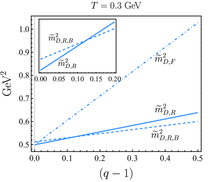
Figure 1: Variation of the non-extensive modified retarded Debye mass $\widetilde{m}_{D,R}^{2}$ (solid line) and non-extensive modified symmetric Debye masses $\widetilde{m}_{D,F}^{2}$ (dot-dashed line) with respect to the non-extensive parameter $q$ for a vanishing magnetic field $eB=0$. The $(q-1)$ dependence of magnetic field-dependent non-extensive modified retarded Debye mass $\widetilde{m}_{D,R,B}^{2}$ (dotted line) is also plotted for $eB=15~{}m_{\pi}^{2}$. In the illustration we compare $\widetilde{m}_{D,R}^{2}$ and $\widetilde{m}_{D,R,B}^{2}$ in the small $(q-1)$ region. All numerical results are performed at a fixed temperature of $T=0.3$ GeV and zero chemical potential.

In figure. 1, we present the non-extensive modified retarded Debye mass $\widetilde{m}_{D,R}^{2}$ and symmetric Debye mass $\widetilde{m}_{D,F}^{2}$ in the zero magnetic field, alongside with the non-extensive modified retarded Debye mass under the finite magnetic field, i.e., $\widetilde{m}_{D,R,B}^{2}$. We observe that all Debye masses monotonically increase with increasing $q$, indicating that the screening effect of the medium is strengthened by non-extensivity. Specially, $\widetilde{m}_{D,R}^{2}$ is smaller than $\widetilde{m}_{D,F}^{2}$, and this difference can be more pronounced at larger $(q-1)$ region. In the absence of non-extensivity, $\widetilde{m}_{D,R,B}^{2}$ is slightly larger than $\widetilde{m}_{D,R}^{2}$, suggesting the screening effect of the medium is increased by the presence of a magnetic field. When both non-extensivity and magnetic field are taken into account, their competing effects determine the final relation between $\widetilde{m}_{D,R}^{2}$ and $\widetilde{m}_{D,R,B}^{2}$. From the illustration in figure. 1, we note that in the small $(q-1)$ region, $\widetilde{m}_{D,R,B}^{2}$ remains slightly larger than $\widetilde{m}_{D,R}$. However, as $(q-1)$ increases further, the non-extensive effect becomes more significant for $\widetilde{m}_{D,R}^{2}$. The steeper slope of $\widetilde{m}_{D,R}^{2}(q-1)$ compared to that of $\widetilde{m}_{D,R,B}^{2}(q-1)$ results in a situation where $\widetilde{m}_{D,R}^{2}$ can overtake the dominance of $\widetilde{m}^{2}_{D,R,B}$ at larger values of $(q-1)$.

Inserting eq. (48) into eq. (39), the temporal component of HTL resummed retarded gluon propagator to the order of $(q-1)^{0}$, $G_{R,(0)}^{*}$, in the zero magnetic field can be determined. It is in the static limit ($\omega\to 0$) written as

$$\underset{\omega\to 0}{\lim}G_{R,(0)}^{*}(Q)=\frac{1}{\widetilde{q}^{2}+m_{D}^{2}}-i\frac{m_{D}^{2}}{2\widetilde{q}}\frac{\pi\omega}{(\widetilde{q}^{2}+m_{D}^{2})^{2}},$$ (101)

which follows from $\underset{\omega\to 0}{\mathrm{lim}}\left[\ln\frac{\omega+\widetilde{q}+i\epsilon}{\omega-\widetilde{q}+i\epsilon}\right]=-i\pi$. By inserting eq. (55) to eq. (40), the non-extensive correction term of temporal component of resummed retarded gluon propagator in the leading order of $(q-1)$, denoted as $G_{R,(1)}^{*}$ within the static limit, is obtained as

$$\underset{\omega\to 0}{\rm lim}G_{R,(1)}^{*}(Q)=-\frac{m_{D,R,(1)}^{2}}{(\widetilde{q}^{2}+m_{D}^{2})^{2}}-i\frac{m_{D,R,(1)}^{2}}{2\widetilde{q}}\frac{(\widetilde{q}^{2}-m_{D}^{2})\omega}{(\widetilde{q}^{2}+m_{D}^{2})^{3}}.$$ (102)

We explicitly determine the temporal component of the resummed symmetric gluon propagator, $G_{F}^{*}$. To facilitate calculation, we will use the following identity:

$$\underset{\omega\to 0}{\mathrm{lim}}(1+2f_{q,B,(0)}(\omega))\mathrm{sgn}(\omega) =\frac{2T}{\omega}+\dots.$$ (103)

Utilizing the set of equations ( (48), (52), (54), (70), (72), and (103)) into eqs. (41) and (2.3), the expressions of $G_{F}^{*}$ up to the order of $(q-1)^{0}$ and $(q-1)$, in the static limit within a zero magnetic field, are respectively derived as

$$\underset{\omega\to 0}{\mathrm{lim}}G_{F,(0)}^{*}(Q) =-i\frac{2\pi T{m}_{D}^{2}}{\widetilde{q}(\widetilde{q}^{2}+{m}_{D}^{2})^{2}},$$ (104)

$$\underset{\omega\to 0}{\mathrm{lim}}G_{F,(1)}^{*}(Q) =-i\frac{m_{D,R,(1)}^{2}}{2\widetilde{q}}\frac{4\pi T(\widetilde{q}^{2}-m_{D}^{2})}{(\widetilde{q}^{2}+m_{D}^{2})^{3}}-i\frac{2\pi T[{m}_{D,F,(1)}^{2}-{m}_{D,R,(1)}^{2}]}{\widetilde{q}(\widetilde{q}^{2}+{m}_{D}^{2})^{2}}.$$ (105)

In the finite magnetic field, inserting eq. (47) and eq. (85) into eq. (39), the temporal component of resummed retarded gluon propagator to order $(q-1)^{0}$, denoted as $G^{*}_{R,B,(0)}$, in the static limit is obtained as

$$\underset{\omega\to 0}{\mathrm{lim}}G^{*}_{R,B,(0)}(Q)= \frac{1}{{\widetilde{q}}^{2}+{m}_{D,B}^{2}}-i\frac{\omega\sum_{f}g^{2}|e_{f}B|)}{4\pi({\widetilde{q}}^{2}+{m}_{D,B}^{2})^{2}}\delta(\widetilde{q}_{z})-i\frac{\omega\pi({m}_{D}^{\rm gluon})^{2}}{2\widetilde{q}({\widetilde{q}}^{2}+{m}_{D,B}^{2})^{2}}$$

$$- i\sum_{f}\sum_{n=1}^{\infty}\sum_{b=\pm}\frac{\omega g^{2}2n|e_{f}B|^{2}H_{b}^{f}(E_{\widetilde{q}_{z}/2,n}^{f})}{4\pi T({\widetilde{q}}^{2}+{m}_{D,B}^{2})^{2}|\widetilde{q}_{z}|E^{f}_{\widetilde{q}_{z}/2,n}}.$$ (106)

Inserting the set of equations ((47), (54), (85), and (86)) into eq. (LABEL:eq:_G^*_R(1)), the correction term of temporal component of resummed retarded gluon propagator to leading order of $(q-1)$, denoted as $G^{*}_{R,B,(1)}$, in the static limit arrives at

$$\underset{\omega\to 0}{\mathrm{lim}}G^{*}_{R,B,(1)}(Q)= -\frac{(m_{D,R,B,(1)}^{\rm quark})^{2}+(m_{D,R,(1)}^{\rm gluon})^{2}}{({\widetilde{q}}^{2}+{m}_{D,B}^{2})^{2}}-i\frac{\omega\pi({m}_{D,R,(1)}^{\rm gluon})^{2}(\widetilde{q}^{2}+m_{D,B}^{2})}{2\widetilde{q}({\widetilde{q}}^{2}+{m}_{D,B}^{2})^{3}}$$

$$+ i\frac{2\omega\pi({m}_{D}^{\rm gluon})^{2}m_{D,R,B,(1)}^{2}}{2\widetilde{q}({\widetilde{q}}^{2}+{m}_{D,B}^{2})^{3}}+i\frac{2\omega\sum_{f}g^{2}|e_{f}B|m_{D,R,B,(1)}^{2}}{4\pi({\widetilde{q}}^{2}+{m}_{D,B}^{2})^{3}}\delta(\widetilde{q}_{z})$$

$$- i\sum_{f}\sum_{n=1}^{\infty}\sum_{b=\pm}\frac{\omega g^{2}2n|e_{f}B|^{2}M_{b}^{f}(E_{\widetilde{q}_{z}/2,n}^{f})}{4\pi T({\widetilde{q}}^{2}+{m}_{D,B}^{2})^{2}|\widetilde{q}_{z}|E^{f}_{\widetilde{q}_{z}/2,n}}\frac{q-1}{2}$$

$$+ i\sum_{f}\sum_{n=1}^{\infty}\sum_{b=\pm}\frac{2\omega g^{|}e_{f}B|^{2}H_{b}^{f}(E_{\widetilde{q}_{z}/2,n}^{f})m_{D,R,B,(1)}^{2}}{4\pi T({\widetilde{q}}^{2}+{m}_{D,B}^{2})^{3}|\widetilde{q}_{z}|E^{f}_{\widetilde{q}_{z}/2,n}}.$$ (107)

Similarly, inserting eq. (106) into eq. (41), the temporal component of resummed symmetric gluon propagator to the order of $(q-1)^{0}$ in the magnetic field, denoted as $G_{F,B,(0)}^{*}$, within the static limit ($\omega\to 0$) is obtained as,

$$\underset{\omega\to 0}{\mathrm{lim}}G_{F,B,(0)}^{*}(Q) =-i\sum_{f}\sum_{n=1}^{\infty}\sum_{b=\pm}\frac{g^{2}8n|e_{f}B|^{2}H_{b}^{f}(E^{f}_{\widetilde{q}_{z}/2,n})}{4\pi({\widetilde{q}}^{2}+m_{D,B}^{2})^{2}|\widetilde{q}_{z}|E^{f}_{\widetilde{q}_{z}/2,n}}-i\frac{2T\pi({m}_{D}^{\rm gluon})^{2}}{\widetilde{q}({\widetilde{q}}^{2}+m_{D,B}^{2})^{2}}.$$ (108)

By inserting the set of equations ((47), (54), (67), (72), (92), (93),(97), (98), (106), and (109)) into eq. (2.3), one finally gets the non-extensive correction term of the temporal component of resummed symmetric gluon propagator to the leading order of $(q-1)$ in a magnetic field, denoted as $G_{F,B,(1)}^{*}$, which in the static limit ($\omega\to 0$) is expressed as

$$\underset{\omega\to 0}{\mathrm{lim}}G_{F,B,(1)}^{*}(Q) =-i\frac{2T\pi({m}_{D,R,(1)}^{\rm gluon})^{2}}{\widetilde{q}({\widetilde{q}}^{2}+{m}_{D,B}^{2})^{2}}-i\frac{2T\pi\left[(m^{\rm gluon}_{D,F,(1)})^{2}-(m^{\rm gluon}_{D,R,(1)})^{2}\right]}{\widetilde{q}({\widetilde{q}}^{2}+{m}_{D,B}^{2})^{2}}$$

$$+i\frac{4T\pi({m}_{D}^{\rm gluon})^{2}m_{D,R,B,(1)}^{2}}{\widetilde{q}({\widetilde{q}}^{2}+{m}_{D,B}^{2})^{3}}+i\frac{8T\sum_{f}g^{2}|e_{f}B|m_{D,R,B,(1)}^{2}}{4\pi({\widetilde{q}}^{2}+{m}_{D,B}^{2})^{3}}\delta(\widetilde{q}_{z})$$

$$+i\sum_{f}\sum_{n=1}^{\infty}\sum_{b=\pm}\frac{g^{2}16n|e_{f}B|^{2}H_{b}^{f}(E^{f}_{\widetilde{q}_{z}/2,n})m_{D,R,B,(1)}^{2}}{4\pi({\widetilde{q}}^{2}+{m}_{D,B}^{2})^{3}|\widetilde{q}_{z}|E^{f}_{\widetilde{q}_{z}/2,n}}$$

$$-i\sum_{f}\sum_{n=1}^{\infty}\sum_{b=\pm}\frac{g^{2}8n|e_{f}B|^{2}W^{f}_{b}(E_{\widetilde{q}_{z}/2,n}^{f})}{4\pi({\widetilde{q}}^{2}+{m}_{D,B}^{2})^{2}|\widetilde{q}_{z}|E_{\widetilde{q}_{z}/2,n}^{f}}\frac{q-1}{2}.$$ (109)

Compared to eq. (108), we note that the term related to the vacuum contribution from quark-loop to the symmetric gluon self-energy is present in the non-extensive correction term.

4 Heavy quark potential in a non-extensive QGP in zero and finite magnetic fields

Applying the non-extensive modified resummed gluon propagator in the static limit, we investigate the in-medium heavy quark potential. This potential describes the interactions between a quark and its antiquark within a QGP and serves as the starting point for non-relativistic approaches to study the in-medium properties of heavy quarkonia. In a vacuum, the heavy quark potential can be well parameterized by the Cornell potential Eichten:1974af ; Matsui:1986dk :

$$V_{\rm Cornell}(r)=-C_{F}\alpha_{s}/r+\sigma r,$$ (110)

where $r\equiv|\bm{r}|$ denotes the separation distance between heavy quark and antiquark, $\alpha_{s}$ represents the strong coupling constant, $C_{F}=(N_{c}^{2}-1)/2N_{c}$, $\sigma$ is the string tension which is determined to reproduce the vacuum quarkonium property Jacobs:1986gv . The first term corresponds to the Coulombic part, reflecting the asymptotic freedom at small separation distances, while the second term represents the string-like part, responsible for color confinement at large separation distances. In the QGP, the in-medium heavy quark potential can be obtained by modifying the vacuum potential with the dielectric permittivity Thakur:2013nia ; Agotiya:2008ie ; Thakur:2016cki .

4.1 Dielectric permittivity

As described in refs. Thakur:2013nia ; Agotiya:2008ie ; Thakur:2016cki , the dielectric permittivity $\varepsilon$, which encodes in-medium effects, such as finite temperature and non-extensive effects, is obtained by using the temporal component of the 11-part of the HTL resummed gluon propagator. It is expressed as

$$\varepsilon^{-1}(\widetilde{{q}})=\lim_{\omega\to 0}\widetilde{q}^{2}G_{11}^{*}(Q)=\lim_{\omega\to 0}\widetilde{q}^{2}\left(G_{R}^{*}(Q)+G_{A}^{*}(Q)+G_{F}^{*}(Q)\right)/2.$$ (111)

By inserting eqs. (101), (102), (104), and (105) into eq. (111), the non-extensive modified dielectric permittivity in the presence of small non-extensivity for vanishing magnetic field can be determined as:

$$\varepsilon^{-1}({\widetilde{q}}) =\frac{\widetilde{q}^{2}}{{\widetilde{q}}^{2}+{m}^{2}_{D}}-\frac{\widetilde{q}^{2}m_{D,R,(1)}^{2}}{({\widetilde{q}}^{2}+{m}^{2}_{D})^{2}}-i\frac{\pi T\widetilde{q}({m}_{D}^{\rm gluon})^{2}}{(\widetilde{q}^{2}+{m}_{D}^{2})^{2}}-i\frac{\pi T\widetilde{q}(\widetilde{q}^{2}-m_{D}^{2})}{(\widetilde{q}^{2}+m_{D}^{2})^{3}}(m_{D,R,(1)}^{\rm gluon})^{2}$$

$$-i\frac{\pi T\widetilde{q}\left[({m}_{D,F,(1)}^{\rm gluon})^{2}-({m}_{D,R,(1)}^{\rm gluon})^{2}\right]}{(\widetilde{q}^{2}+{m}_{D}^{2})^{2}}-i\frac{\pi T\widetilde{q}({m}_{D}^{\rm quark})^{2}}{(\widetilde{q}^{2}+{m}_{D}^{2})^{2}}-i\frac{\pi T\widetilde{q}(\widetilde{q}^{2}-m_{D}^{2})}{(\widetilde{q}^{2}+m_{D}^{2})^{3}}(m_{D,R,(1)}^{\rm quark})^{2}$$

$$-i\frac{\pi T\widetilde{q}\left[({m}_{D,F,(1)}^{\rm quark})^{2}-({m}_{D,R,(1)}^{\rm quark})^{2}\right]}{(\widetilde{q}^{2}+{m}_{D}^{2})^{2}}.$$ (112)

As $q$ approaches 1, ${m}_{D,R,(1)}^{\rm quark/gluon}$ and ${m}_{D,F,(1)}^{\rm quark/gluon}$ vanish, then the extensive equilibrium form of $\varepsilon^{-1}$ is reproduced. Similarly, by putting eqs. (106), (107), (108), and (109) into eq. (111), the non-extensive modified dielectric permittivity for the finite magnetic field is written as

$$\varepsilon^{-1}_{B}({\widetilde{q}})= \frac{\widetilde{q}^{2}}{{\widetilde{q}}^{2}+{m}_{D,B}^{2}}-\frac{\widetilde{q}^{2}m_{D,R,B,(1)}^{2}}{({\widetilde{q}}^{2}+{m}_{D,B}^{2})^{2}}-i\frac{\pi T\widetilde{q}({m}_{D}^{\rm gluon})^{2}}{({\widetilde{q}}^{2}+m_{D,B}^{2})^{2}}-i\frac{\pi T\widetilde{q}(m^{\rm gluon}_{D,F,(1)})^{2}}{({\widetilde{q}}^{2}+{m}_{D,B}^{2})^{2}}$$

$$+ i\frac{2\pi T\widetilde{q}({m}_{D}^{\rm gluon})^{2}m_{D,R,B,(1)}^{2}}{({\widetilde{q}}^{2}+{m}_{D,B}^{2})^{3}}-i\sum_{f}\sum_{n=1}^{\infty}\sum_{b=\pm}\frac{\alpha_{s}4n|e_{f}B|^{2}H_{b}^{f}(E^{f}_{\widetilde{q}_{z}/2,n})\widetilde{q}^{2}}{({\widetilde{q}}^{2}+m_{D,B}^{2})^{2}|\widetilde{q}_{z}|E^{f}_{\widetilde{q}_{z}/2,n}}$$

$$+ i\frac{4T\sum_{f}\alpha_{s}|e_{f}B|m_{D,R,B,(1)}^{2}\widetilde{q}^{2}}{({\widetilde{q}}^{2}+{m}_{D,B}^{2})^{3}}\delta(\widetilde{q}_{z})$$

$$+ i\sum_{f}\sum_{n=1}^{\infty}\sum_{b=\pm}\frac{\alpha_{s}8n|e_{f}B|^{2}H_{b}^{f}(E^{f}_{\widetilde{q}_{z}/2,n})m_{D,R,B,(1)}^{2}\widetilde{q}^{2}}{({\widetilde{q}}^{2}+{m}_{D,B}^{2})^{3}|\widetilde{q}_{z}|E^{f}_{\widetilde{q}_{z}/2,n}}$$

$$- i\sum_{f}\sum_{n=1}^{\infty}\sum_{b=\pm}\frac{\alpha_{s}4n|e_{f}B|^{2}W^{f}_{b}(E_{\widetilde{q}_{z}/2,n}^{f})\widetilde{q}^{2}}{({\widetilde{q}}^{2}+{m}_{D,B}^{2})^{2}|\widetilde{q}_{z}|E_{\widetilde{q}_{z}/2,n}^{f}}\frac{q-1}{2}.$$ (113)

4.2 Real part of in-medium heavy quark potential

Following the approach proposed in Thakur:2013nia ; Agotiya:2008ie ; Thakur:2016cki , the in-medium heavy quark potential in the non-extensive QGP can be determined through the convolution of the Cornell potential and the non-extensive modified dielectric permittivity,

$$V({\widetilde{q}})=V_{\rm Cornell}({\widetilde{q}})\varepsilon^{-1}({\widetilde{q}}).$$ (114)

Here, the Fourier transform of the Cornell potential in the momentum space, $V_{\rm Cornell}({\widetilde{q}})$, is given as Thakur:2013nia

$$V_{\rm Cornell}(\widetilde{q})=-\sqrt{(2/\pi)}\frac{C_{F}\alpha_{s}}{\widetilde{q}^{2}}-\frac{4\sigma}{\sqrt{2\pi}\widetilde{q}^{4}}.$$ (115)

Through the Fourier transform, eq. (114) is transformed into real coordinate space, which is expressed as

$$V(\bm{r}) = \int\frac{d^{3}\bm{\widetilde{q}}}{{(2\pi)}^{3/2}}(e^{i\bm{\widetilde{\bm{q}}}\cdot\bm{r}}-1)~{}\frac{V_{\rm Cornell}(\widetilde{q})}{\varepsilon({\widetilde{q}})}.$$ (116)

Without loss of generality, $\widetilde{\bm{q}}$ and $\bm{r}$ are chosen as $\bm{\widetilde{q}}=\widetilde{q}(\sin\theta\cos\phi,\sin\theta\sin\phi,\cos\theta)$ and $\bm{r}=r(\sin\chi,0,\cos\chi)$, respectively. Here, $\chi$ denotes the angle between $\bm{\widetilde{q}}$ and $\bm{r}$. The dot product $\bm{\widetilde{q}}\cdot\bm{r}$ is given by $\widetilde{q}r(\sin\chi\cos\phi\sin\theta+\cos\chi\cos\theta)$. Consequently, eq. (116) can be rewritten as

$$V(r,\chi,q,T,eB)=\int\frac{\widetilde{q}^{2}\sin\theta d\theta d\widetilde{q}}{(2\pi)^{1/2}}\left[J_{0}(\widetilde{q}r\sin\theta\sin\chi)e^{i\widetilde{q}r\cos\theta\cos\chi}-1\right]V({\widetilde{q}}),$$ (117)

where $J_{m}(x)$ is the Bessel function of the first kind.

In the present work, the string tension is chosen as $\sigma=0.18~{}\mathrm{GeV}^{2}$ Satz:2005hx . The running strong coupling strength $g$ is obtained from Ayala:2018wux

$$\alpha_{s}(\Lambda^{2},eB)=\frac{g^{2}}{4\pi}=\frac{\alpha_{s}(\Lambda^{2})}{1+\frac{11N_{c}-2N_{f}}{12\pi}\alpha_{s}(\Lambda^{2})\ln(\frac{\Lambda^{2}}{\Lambda^{2}+eB})},$$ (118)

where the one-loop QCD strong coupling constant $\alpha_{s}$ for $eB=0$ is given as $\alpha_{s}(\Lambda^{2})=g^{2}/(4\pi)=\frac{12\pi}{11N_{c}-2N_{f}}\ln\frac{\Lambda_{\bar{MS}}^{2}}{\Lambda^{2}}$ at $\Lambda_{\bar{MS}}=176~{}\mathrm{MeV}$ for $N_{f}=N_{c}=3$. The scale $\Lambda$ is taken as $2\pi\sqrt{T^{2}+\mu^{2}/\pi^{2}}$ for quarks and $2\pi T$ for gluons, $b_{1}=\frac{11N_{c}-2N_{f}}{12\pi}$ and $\Lambda_{\bar{MS}}=176~{}\mathrm{MeV}$ Bazavov:2012ka .

By inserting the real part of eq. (112) into eq. (117), we compute the real part of the potential, denoted as $\mathrm{Re}\,V$, in the absence of a magnetic field. The extensive contribution of $\mathrm{Re}\,V$ is then obtained as follows:

$$\mathrm{Re}\,V_{(0)}(r,T) =\mathrm{Re}\,V_{\rm HTL,(0)}(r,T)+\mathrm{Re}\,V_{\rm string,(0)}(r,T)$$ (119)

$$=-C_{F}\alpha_{s}\,{m}_{D}\left(\frac{e^{-{m}_{D}\,r}}{{m}_{D}\,r}+1\right)+\frac{2\sigma}{{m}_{D}}\left(\frac{e^{-{m}_{D}\,{r}}-1}{{m}_{D}\,r}+1\right).$$ (120)

The non-extensive correction term of $\mathrm{Re}\,V$ in the leading order of $(q-1)$ is obtained as

$$\mathrm{Re}\,V_{(1)}(r,q,T) =\mathrm{Re}\,V_{\rm HTL,(1)}(r,q,T)+\mathrm{Re}\,V_{\rm string,(1)}(r,q,T)$$ (121)

$$=C_{F}\alpha_{s}\frac{m_{D,R,(1)}^{2}}{2m_{D}}\left(e^{-m_{D}r}-1\right)$$

$$+\frac{\sigma m_{D,R,(1)}^{2}}{m_{D}^{3}}\left(\frac{2-(2+m_{D}r)e^{-m_{D}r}}{m_{D}r}-1\right).$$ (122)

Similarly, by inserting the real part of eq. (113) into eq. (117), the $\mathrm{Re}V$ in the presence of a magnetic field is also computed, and its extensive contribution can be written as

$$\mathrm{Re}\,V_{(0)}(r,T,eB) =\mathrm{Re}\,V_{\rm HTL,(0)}(r,T,eB)+\mathrm{Re}\,V_{\rm string,(0)}(r,T,eB)$$ (123)

$$=-C_{F}\alpha_{s}\,{m}_{D,B}\left(\frac{e^{-{m}_{D,B}\,r}}{{m}_{D,B}\,r}+1\right)+\frac{2\sigma}{{m}_{D,B}}\left(\frac{e^{-{m}_{D,B}\,{r}}-1}{{m}_{D,B}\,r}+1\right).$$ (124)

In the leading order of $(q-1)$, its non-extensive correction term is obtained as

$$\mathrm{Re}\,V_{(1)}(r,q,T,eB) =\mathrm{Re}\,V_{\rm HTL,(1)}(r,q,T,eB)+\mathrm{Re}\,V_{\rm string,(1)}(r,q,T,eB),$$ (125)

$$=C_{F}\alpha_{s}\frac{m_{D,R,B,(1)}^{2}}{2m_{D,B}}\left(e^{-m_{D,B}r}-1\right)$$

$$+\frac{\sigma m_{D,R,B,(1)}^{2}}{m_{D,B}^{3}}\left(\frac{2-(2+m_{D,B}r)e^{-m_{D,B}r}}{m_{D,B}r}-1\right).$$ (126)

The first and second terms on the right side of eqs. (119)-(126) are the HTL and string-like parts of the potential, which are related to the short-range perturbative Yukawa and long-range non-perturbative color confining or string-like interactions between heavy quarks and the QGP medium, respectively. It is clear that by transforming $m_{D}$ and $m_{D,R,(1)}$ in eq. (120) and eq. (122) to $m_{D,B}$ and $m_{D,R,B,(1)}$, respectively, we can arrive at eq. (124) and eq. (126).

In figure. 2, we plot the real part of the heavy quark potential, $\mathrm{Re}\,V$, for different values of non-extensive parameter $q$ with varying quark-antiquark separation distances $r$ in both $eB=0$ (solid lines) and $eB=15~{}m_{\pi}^{2}$ (dashed lines). The magnetic field influences $\mathrm{Re}\,V$ by affecting the quark contribution to the gluon self-energy and the QCD coupling constant. The non-extensive correction alters $\mathrm{Re}\,V$ by modifying the Debye masses, transforming $m_{D}$ and $m_{D,B}$ into $\widetilde{m}_{D,R}$ and $\widetilde{m}_{D,R,B}$, respectively. In the absence of non-extensivity, we observe that the $\mathrm{Re}\,V$ flattens as $r$ increases. Furthermore, the HTL component of $\mathrm{Re}\,V$ ($\mathrm{Re}\,V_{\rm HTL}$) is more screened in a non-zero magnetic field compared to that in a zero magnetic field, whereas the magnetic field dependence of the string component of $\mathrm{Re}\,V$ ($\mathrm{Re}\,V_{\rm string}$) is insignificant, especially in the range $B=0$ to $eB=15~{}m_{\pi}^{2}$. Furthermore, introducing non-extensivity cannot change the qualitative behavior of $\mathrm{Re}\,V$ with $r$. Higher values of $q$ lead to a shorter Debye screening length (or equivalently, a larger Debye screening mass), which results in both $\mathrm{Re}\,V_{\rm HTL}$ and $\mathrm{Re}\,V_{\rm string}$ becoming flatter with increasing $q$ in both the absence and presence of a magnetic field, as shown in the upper panel of figure 2. We also note that, compared to $\mathrm{Re}\,V_{\rm string}$, $\mathrm{Re}\,V_{\rm HTL}$ is more sensitive to the variation in $q$. At $q=1.2$, the difference between $\mathrm{Re}\,V_{\rm HTL}$ for zero magnetic field and finite magnetic field becomes smaller, which can be understood from the left panel of figure 2. Here, the slope of $\mathrm{Re}\,V_{\rm HTL}$ with $q-1$ at a fixed distance in the absence of a magnetic field is steeper than that in the presence of a magnetic field, meaning the variation in $\mathrm{Re}\,V_{\rm HTL}$ due to non-extensive correction in the absence of a magnetic field is more significant. When $(q-1)$ increases further, the $\mathrm{Re}V_{\rm HTL}$ in the absence of a magnetic field can exceed that in the presence of a magnetic field. The slope of $\mathrm{Re}V_{\rm string}$ with respect to $(q-1)$ is qualitatively similar to that of $\mathrm{Re}V_{\rm HTL}$, as shown in the middle panel of figure 2. However, for $q\leq 1.2$, the difference between $\mathrm{Re}\,V_{\rm string}$ with and without a magnetic field is minimal and an over point is located about at $(q-1)=0.1$. When $(q-1)$ increases further, the $\mathrm{Re}\,V_{\rm string}$ in the absence of a magnetic field also can exceed that in the presence of a magnetic field. Due to the overwhelming contribution of $\mathrm{Re}\,V_{\rm string}$ in quantitative, the $\mathrm{Re}\,V$ experiences a slight increase with $q$, and the magnetic field has an insignificant effect in the region of interest where $(q-1)\leq 0.2$, which is clearly shown in the right panel of figure. 2.

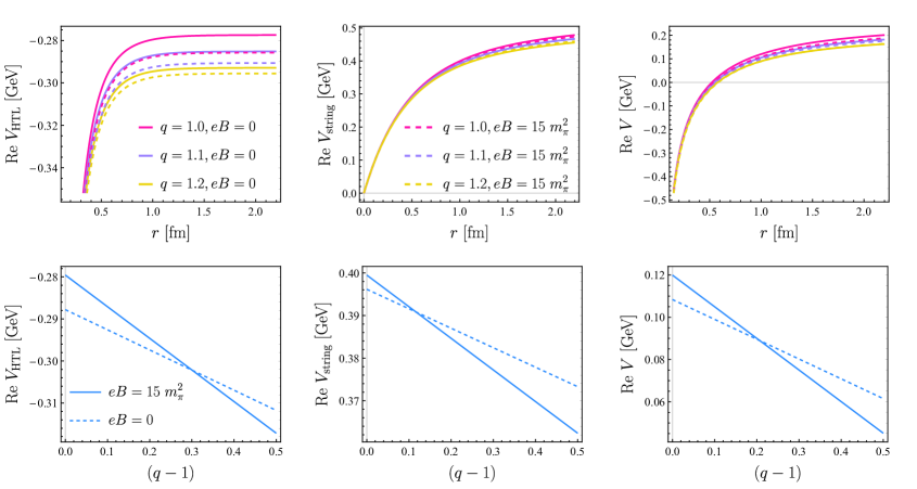
Figure 2: (Upper panel) The HTL component (left), string component (middle), and total component (right) of the real part of heavy quark potential, $\mathrm{Re}\,V$, as functions of quark-antiquark separation distance $r$ at different values of non-extensive parameter $q$. (Lower panel) The $(q-1)$ dependence of $\mathrm{Re}\,V_{\rm HTL}$ (left), $\mathrm{Re}\,V_{\rm string}$ (middle) and $\mathrm{Re}\,V$ (right) for a fixed separation distance $r=1~{}\mathrm{fm}$ and a fixed temperature $T=0.3$ GeV. The solid lines and dashed lines represent the results for the zero magnetic field and for the finite magnetic field with $eB=15~{}m_{\pi}^{2}$, respectively.

4.3 Imaginary part of in-medium heavy quark potential

Next, we study the imaginary part of in-medium heavy quark potential, denoted as $\mathrm{Im}V$, which relates physically to the inelastic scattering of the light constituents of the medium with heavy quarkonium via exchanged gluons (Landau damping phenomenon) in HTL resummed perturbation theory Brambilla:2011sg . A larger magnitude of $\mathrm{Im}\,V$ could trigger a broadening decay width for quarkonium states, which plays an important role in quarkonium dissociation. Since the gluonic and quark contributions to the gluon self-energy, particularly in a finite magnetic field are strikingly different in form, we will separately analyze their respective contributions to the $\mathrm{Im}\,V$, to better elucidate the qualitative features of the potential. Accordingly, the $\mathrm{Im}\,V$ can be decomposed into $\mathrm{Im}\,V=\mathrm{Im}\,V^{\mathrm{gluon}}+\mathrm{Im}\,V^{\mathrm{quark}}$.

Let us first look at the imaginary part of the potential associated with the gluonic contribution to gluon self-energy, denoted as $\mathrm{Im}\,V^{\rm gluon}$. By inserting the third term in the right-hand side of eq. (112) to eq. (116), its extensive part in a zero magnetic field is computed as

$$\mathrm{Im}\,V^{\rm gluon}_{(0)}(r,T) =\mathrm{Im}\,V_{\rm HTL,(0)}^{\rm gluon}(r,T)+\mathrm{Im}\,V_{\rm string,(0)}^{\rm gluon}(r,T)$$ (127)

$$=-C_{F}\alpha_{s}T\frac{({m}_{D}^{\rm gluon})^{2}}{{m}_{D}^{2}}\phi_{2}({m}_{D}r)-\frac{2\sigma T({m}_{D}^{\rm gluon})^{2}}{{m}_{D}^{4}}\chi_{2}({m}_{D}r).$$ (128)

Then, inserting the fourth and fifth terms in the right-hand side of eq. (112) to eq. (116), the non-extensive correction term of $\mathrm{Im}\,V^{\rm gluon}$ in a zero magnetic field is obtained as

$$\mathrm{Im~{}V}^{\rm gluon}_{(1)}(r,q,T) =\mathrm{Im}V_{\rm HTL,(1)}^{\rm gluon}(r,q,T)+\mathrm{Im}V_{\rm string,(1)}^{\rm gluon}(r,q,T),$$ (129)

$$=-C_{F}\alpha_{s}T\bigg{[}\frac{(m_{D,R,(1)}^{\rm gluon})^{2}}{m_{D}^{2}}\bigg{(}\psi(m_{D}r)-\phi_{2}(m_{D}r)-\phi_{3}(m_{D}r)\bigg{)}$$

$$+\frac{(m_{D,F,(1)}^{\rm gluon})^{2}}{{m}_{D}^{2}}\phi_{2}({m}_{D}r)\bigg{]}-\frac{2\sigma T}{m_{D}^{2}}\bigg{[}\frac{(m_{D,F,(1)}^{\rm gluon})^{2}}{{m}_{D}^{2}}\chi_{2}({m}_{D}r)$$

$$+\frac{({m}_{D,R,(1)}^{\rm gluon})^{2}}{{m}_{D}^{2}}\bigg{(}\phi_{3}(m_{D}r)-\chi_{2}(m_{D}r)-\chi_{3}(m_{D}r)\bigg{)}\bigg{]}.$$ (130)

In the presence of a magnetic field, by inserting eq. (113) to eq. (116), $\mathrm{Im}V_{(0)}^{\rm gluon}$ and $\mathrm{Im}V_{(1)}^{\rm gluon}$ are computed as

$$\mathrm{Im}\,V_{(0)}^{\rm gluon}(r,T,eB) =\mathrm{Im}\,V_{\rm HTL,(0)}^{\rm gluon}(r,T,eB)+\mathrm{Im}\,V_{\rm string,(0)}^{\rm gluon}(r,T,eB)$$ (131)

$$=-C_{F}\alpha_{s}T\frac{({m}_{D}^{\rm gluon})^{2}}{{m}_{D,B}^{2}}\phi_{2}({m}_{D,B}r)-\frac{2\sigma T({m}_{D}^{\rm gluon})^{2}}{{m}_{D,B}^{4}}\chi_{2}({m}_{D,B}r),$$ (132)

and

$$\mathrm{Im}\,V_{(1)}^{\rm gluon}(r,q,T,eB) =\mathrm{Im}\,V_{\rm HTL,(1)}^{\rm gluon}(r,q,T,eB)+\mathrm{Im}\,V_{\rm string,(1)}^{\rm gluon}(r,q,T,eB)$$ (133)

$$=-C_{F}\alpha_{s}T\bigg{[}\frac{(m_{D,F,(1)}^{\rm gluon})^{2}}{{m}_{D,B}^{2}}\phi_{2}({m}_{D,B}r)$$

$$-\frac{2m_{D,R,B,(1)}^{2}(m_{D}^{\rm gluon})^{2}}{m_{D,B}^{4}}\phi_{3}(m_{D,B}r)\bigg{]}-\frac{2\sigma T}{m_{D,B}^{2}}\bigg{[}\frac{(m_{D,F,(1)}^{\rm gluon})^{2}}{{m}_{D,B}^{2}}\chi_{2}({m}_{D,B}r)$$

$$-\frac{2{m}_{D,R,B,(1)}^{2}({m}_{D}^{\rm gluon})^{2}}{{m}_{D,B}^{4}}\chi_{3}(m_{D,B}r)\bigg{]},$$ (134)

respectively. It is clear that eq. (132) is formally consistent with eq. (128) except for the Debye mass. The functions $\phi_{n}(x)$ and $\chi(x)$ are defined by $\phi_{n}(x)\equiv 2\int_{0}^{\infty}dz\frac{z}{(z^{2}+1)^{n}}\left[1-\frac{\sin(xz)}{xz}\right]$, $\chi_{n}(x)\equiv 2\int_{0}^{\infty}\frac{dz}{z(z^{2}+1)^{n}}\left[1-\frac{\sin(xz)}{xz}\right]$, respectively, as well as $\psi(x)=2\int_{0}^{\infty}\frac{z^{3}}{(z+1)^{3}}\left[1-\frac{\sin(xz)}{xz}\right]$. Comparing eq. (130) and eq. (134), we note that the non-extensive correction terms of $\mathrm{Im}\,V^{\rm gluon}$ in the absence and presence of the magnetic field are different.

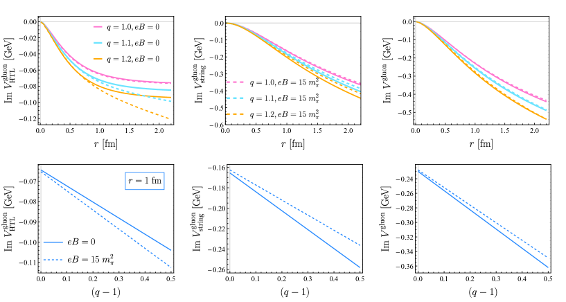
Figure 3: Same as figure. 2 but for the different components of the imaginary part of the potential originated from the gluonic contribution to the gluon self-energy, $\mathrm{Im}\,V^{\rm gluon}$.

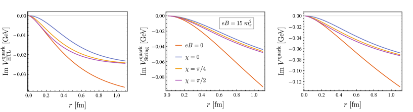
Figure 4: The HTL component (left), string component (middle), and total component (right) of the imaginary part of heavy quark potential originating from quark contribution to gluon self-energy, $\mathrm{Im}\,V^{\rm quark}$, as a function of quark-antiquark separation distance $r$ in $eB=0$ and $eB=15~{}m_{\pi}^{2}$ with $\chi=0,\pi/4,\pi/2$.

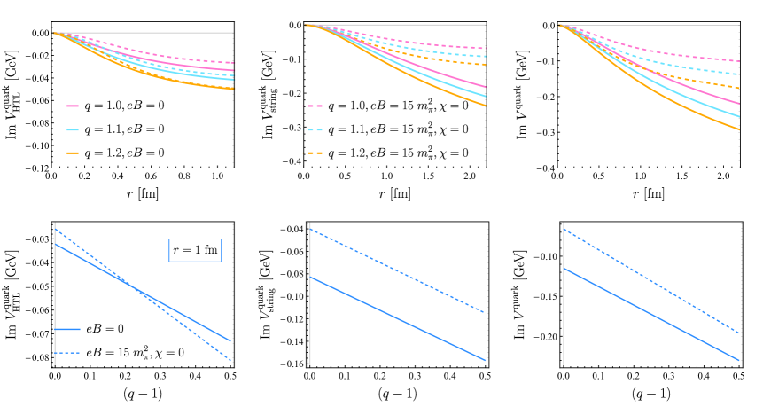
Figure 5: Same as figure. 2 but for the different components of $\mathrm{Im}\,V^{\rm quark}$. The solid lines and dashed lines represent the results for the vanishing magnetic field and the finite magnetic field $eB=15~{}m_{\pi}^{2}$ with $\chi=0$, respectively.

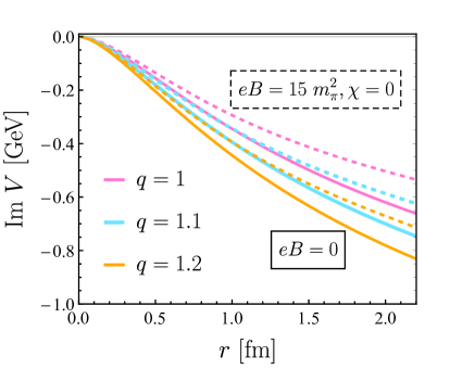
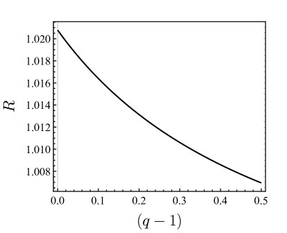
Figure 6: (Left panel) The variation of the total imaginary part of the heavy quark potential, $\mathrm{Im}\,V$, with quark-antiquark separation distance $r$ for different values of $q$ at a fixed temperature $T=0.3$ GeV. The solid lines represent the results for the vanishing magnetic field, while the dashed lines represent the results for the finite magnetic field $eB=15~{}m_{\pi}^{2}$ with $\chi=0$, respectively. (Right panel) The anisotropy ratio of $\mathrm{Im}V$, defined as $R=\mathrm{Im}\,V(r,\chi=\pi/2,q,T,eB)/\mathrm{Im}\,V(r,\chi=0,q,T,eB)$ is plotted as a function of $(q-1)$ at $r=1~{}$fm.

In the upper panel of figure. 3, we show the dependence of the imaginary part of in-medium heavy quark potential related to the gluonic contribution of gluon self-energy, $\mathrm{Im}V^{\rm gluon}$, on the quark-antiquark separation distance $r$ at different values of non-extensive parameter $q$. Results are presented for $eB=0$ (solid lines) and $eB=15~{}m_{\pi}^{2}$ (dashed lines) at $T=0.3~{}$GeV. It is clear that the magnitudes of both the HTL and string components of $\mathrm{Im}\,V^{\rm gluon}$ exhibit an increasing trend with $r$ and $q$. Specifically, the $\mathrm{Im}\,V_{\rm HTL}^{\rm gluon}$ dominates in the small $r$ region due to $\phi_{2}\sim r^{2}\ln r$ and $\chi_{2}\sim r^{2}$ to leading order, while the $\mathrm{Im}\,V_{\rm string}^{\rm gluon}$, dominates in the large $r$ region. In the absence of non-extensity, the magnetic field dependence of $\mathrm{Im}\,V^{\rm gluon}$ is also minimal. When the non-extensive correction is considered, the magnetic field effect significantly enhances the magnitude of $\mathrm{Im}\,V_{\rm HTL}^{\rm gluon}$ but weakly lowers the magnitude of $\mathrm{Im}\,V_{\rm string}^{\rm gluon}$. These variations become more pronounced with increasing $q$, as illustrated in the lower panel of figure. 3. The $(q-1)$ dependence of both HTL and string components for $\mathrm{Im}\,V^{\rm gluon}$ remains unchanged by the magnetic field. Due to the opposite responses of $\mathrm{Im}\,V_{\rm HTL}^{\rm gluon}$ and $\mathrm{Im}\,V_{\rm string}^{\rm gluon}$ to the magnetic field, the difference between the $\mathrm{Im}\,V^{\rm gluon}$ in zero and finite magnetic fields is still insignificant at both $q=1.1$ and $q=1.2$. As $q$ further increases, this difference can slightly enlarge, as depicted in the lower panel of figure. 3.

Next, we examine the non-extensive correction to the imaginary part of the heavy quark potential originating from the quark contribution to gluon self-energy, $\mathrm{Im}\,V^{\rm quark}$, both in the absence and presence of a magnetic field. By inserting the sixth term from the right-hand side of eq. (112) into eq. (116), the extensive part of $\mathrm{Im}\,V^{\rm quark}$, in the absence of a magnetic field is computed as

$$\mathrm{Im}\,V_{(0)}^{\rm quark}(r,T) =\mathrm{Im}\,V_{\rm HTL,(0)}^{\rm quark}(r,T)+\mathrm{Im}\,V_{\rm string,(0)}^{\rm quark}(r,T)$$ (135)

$$=-C_{F}\alpha_{s}T\frac{({m}_{D}^{\rm quark})^{2}}{{m}_{D}^{2}}\phi_{2}({m}_{D}r)-\frac{2\sigma T({m}_{D}^{\rm quark})^{2}}{{m}_{D}^{4}}\chi_{2}({m}_{D}r).$$ (136)

Putting the seventh and eighth terms from the right-hand side of eq. (112) into eq. (116), the non-extensive correction term of $\mathrm{Im}\,V^{\rm quark}$ up to the order of ($q-1$), arrives at

$$\mathrm{Im}\,V_{(1)}^{\rm quark}(r,q,T) =\mathrm{Im}\,V_{\rm HTL,(1)}^{\rm quark}(r,q,T)+\mathrm{Im}\,V_{\rm string,(1)}^{\rm quark}(r,q,T)$$ (137)

$$=-C_{F}\alpha_{s}T\bigg{[}\frac{(m_{D,R,(1)}^{\rm quark})^{2}}{m_{D}^{2}}\bigg{(}\psi(m_{D}r)-\phi_{2}(m_{D}r)-\phi_{3}(m_{D}r)\bigg{)}$$

$$+\frac{(m_{D,F,(1)}^{\rm quark})^{2}}{{m}_{D}^{2}}\phi_{2}({m}_{D}r)\bigg{]}-\frac{2\sigma T}{m_{D}^{2}}\bigg{[}\frac{(m_{D,F,(1)}^{\rm quark})^{2}}{{m}_{D}^{2}}\chi_{2}({m}_{D}r)$$

$$+\frac{({m}_{D,R,(1)}^{\rm quark})^{2}}{{m}_{D}^{2}}\bigg{(}\phi_{3}(m_{D}r)-\chi_{2}(m_{D}r)-\chi_{3}(m_{D}r)\bigg{)}\bigg{]}.$$ (138)

Similarly, inserting the sixth term from the right-hand side of eq. (113) into eq. (116), the extensive part of $\mathrm{Im}V^{\rm quark}$ in the presence of a magnetic field is computed as follows:

$$\mathrm{Im}\,V_{(0)}^{\rm quark}(r,\chi,T,eB) =\mathrm{Im}\,V_{\rm HTL,(0)}^{\rm quark}(r,\chi,T,eB)+\mathrm{Im}\,V_{\rm string,(0)}^{\rm quark}(r,\chi,T,eB)$$ (139)

$$=\int\widetilde{q}^{2}\sin\theta d\theta d\widetilde{q}\left[J_{0}(\widetilde{q}r\sin\theta\sin\chi)e^{i\widetilde{q}r\cos\theta\cos\chi}-1\right]$$

$$\times\left[\sum_{f}\sum_{n=1}^{\infty}\sum_{b=\pm}\frac{\alpha_{s}4n|e_{f}B|^{2}H^{f}_{b}(E_{\widetilde{q}_{z}/2,n}^{f})}{({\widetilde{q}}^{2}+m_{D,B}^{2})^{2}|\widetilde{q}_{z}|E^{f}_{\widetilde{q}_{z}/2,n}}\right]\left(\frac{C_{F}\alpha_{s}}{\pi}+\frac{2\sigma}{\widetilde{q}^{2}\pi}\right).$$ (140)

By inserting the seventh, eighth, and ninth terms from the right-hand side of eq. (113) into eq. (116), we obtain the non-extensive correction term of $\mathrm{Im}V^{\rm quark}$ in the presence of the magnetic field, up to leading order of ($q-1$), which is written as

$$\mathrm{Im}\,V_{(1)}^{\rm quark}(r,\chi,q,T,eB) =\mathrm{Im}\,V^{\rm quark}_{\rm HTL,(1)}(r,\chi,q,T,eB)+\mathrm{Im}\,V^{\rm quark}_{\rm string,(1)}(r,\chi,q,T,eB)$$ (141)

$$=\int\widetilde{q}^{2}\sin\theta d\theta d\widetilde{q}\left[J_{0}(\widetilde{q}r\sin\theta\sin\chi)e^{i\widetilde{q}r\cos\theta\cos\chi}-1\right]$$

$$\times\bigg{\{}\sum_{f}\sum_{n=1}^{\infty}\sum_{b=\pm}\frac{\alpha_{s}4n|e_{f}B|^{2}}{({\widetilde{q}}^{2}+m_{D,B}^{2})^{2}|\widetilde{q}_{z}|E^{f}_{\widetilde{q}_{z}/2,n}}\bigg{[}W^{f}_{b}(E_{\widetilde{q}_{z}/2,n}^{f})\frac{q-1}{2}$$

$$-\frac{2H_{b}^{f}(E_{\widetilde{q}_{z}/2,n}^{f})m_{D,R,B,(1)}^{2}}{\widetilde{q}^{2}+m_{D,B}^{2}}\bigg{]}\bigg{\}}\left(\frac{C_{F}\alpha_{s}}{\pi}+\frac{2\sigma}{\widetilde{q}^{2}\pi}\right)$$

$$-\frac{C_{F}\alpha_{s}T}{2\pi}\frac{\sum_{f}\alpha_{s}|e_{f}B|m_{D,R,B,(1)}^{2}}{m_{D,B}^{4}}$$

$$\times\bigg{[}m_{D,B}^{2}r^{2}K_{2}(m_{D,B}r\sin\chi)(\sin\chi)^{2}-2\bigg{]}$$

$$-\frac{4\sigma T}{\pi}\int d\widetilde{q}\left[J_{0}(\widetilde{q}r\sin\chi)-1\right]\frac{\sum_{f}\alpha_{s}|e_{f}B|m_{D,R,B,(1)}^{2}}{\widetilde{q}(\widetilde{q}^{2}+m_{D,B}^{2})^{3}}.$$ (142)

Here, $E_{\widetilde{q}_{z}/2,n}^{f}$ needs to rewrite as $E_{\widetilde{q}_{z}/2,n}^{f}=\sqrt{(\widetilde{q}\cos\theta/2)^{2}+2n|e_{f}B|}$ and $K_{m}(x)$ is the Bessel function of the second kind. It is noted that $\mathrm{Im}\,V^{\rm quark}=\mathrm{Im}\,V_{(0)}^{\rm quark}+\mathrm{Im}\,V_{(1)}^{\rm quark}$ in a magnetic field becomes directional or angular $\chi$ dependent.

In figure. 4, we show the angular dependence of each component of $\mathrm{Im}\,V^{\rm quark}$ in the presence of a magnetic field $eB=15~{}m_{\pi}^{2}$. As illustrated in figure. 4, both HTL and string components of $|\mathrm{Im}\,V^{\rm quark}|$ exhibit a maximum at $\chi=\pi/2$, where the quark-antiquark dipole is aligned perpendicular to the magnetic field direction. Conversely, a minimum is observed at $\chi=0$, where the quark-antiquark dipole is parallel to the magnetic field direction. This observation confirms the anisotropy of $\mathrm{Im}\,V^{\rm quark}$ in a magnetic field. Furthermore, including a magnetic field significantly suppresses the magnitude of $\mathrm{Im}\,V^{\rm quark}$. Quantitatively, the decreasing trend in each component of $|\mathrm{Im}\,V^{\rm quark}|$ with increasing $r$ is similar, both in the absence and presence of a magnetic field.

Based above, in figure. 5, we plot the separation distance $r$ dependence of each component of $\mathrm{Im}\,V^{\rm quark}$ in the zero magnetic field at different values of $q$, and compare with the corresponding numerical results in $eB=15~{}m_{\pi}^{2}$ with the case of $\chi=0$. In both zero and magnetic fields, the HTL and string components of $|\mathrm{Im}\,V^{\rm quark}|$ increase as $q$ increases, as observed from their $q$-dependence at a fixed distance in the lower panel of figure. 5. When considering the non-extensive correction, as shown in the upper panel of figure. 5, we see that the suppression of $|\mathrm{Im}\,V^{\rm quark}_{\rm HTL}|$ by the magnetic field is less pronounced at $q=1.1$ compared to $q=1$. At $q=1.2$, the curves for $\mathrm{Im}\,V^{\rm quark}_{\rm HTL}$ in the absence and presence of a magnetic field almost overlap. This minimal difference can be attributed to the steeper slope of $\mathrm{Im}\,V^{\rm quark}_{\rm HTL}$ with $q$ in a magnetic field, as illustrated in the lower-left panel of figure. 5. Consequently, the magnitude of $\mathrm{Im}\,V^{\rm quark}_{\rm HTL}$ for a fixed distance of $1$ fm surpasses that in the absence of a magnetic field at $q>1.2$. Unlike $\mathrm{Im}\,V^{\rm quark}_{\rm HTL}$, $\mathrm{Im}\,V^{\rm quark}_{\rm string}$ exhibits a consistently lower magnitude in the presence of a magnetic field at different values of $q$, as evident from the middle panel of figure. 5. Combining the HTL and string components, as shown in the right panel of figure. 5, the magnitude of $\mathrm{Im}\,V^{\rm quark}$ in the presence of a magnetic field remains smaller than that in the absence of a magnetic field, regardless of the non-extensive correction.

In the left panel of figure. 6, we present the behavior of the total imaginary part of the potential, $\mathrm{Im}V$, with separation distance $r$ in both zero (solid lines) and finite magnetic field with the case of $\chi=0$ (dashed lines). As $q$ and $r$ increase, the magnitudes of both $\mathrm{Im}\,V^{\rm gluon}$ and $\mathrm{Im}\,V^{\rm quark}$ increase, leading to a continuous increase in $|\mathrm{Im}V|$. In the presence of a magnetic field, the magnitude of $\mathrm{Im}V$ for different $q$ values is smaller compared to that in the purely thermal case. In the right panel of figure. 6, we present the anisotropy ratio $R$ of the $\mathrm{Im}\,V$ to quantify its anisotropic response to the magnetic field and non-extensive correction. After accounting for the isotropic contribution from $\mathrm{Im}V^{\rm gluon}$, the anisotropic feature of $\mathrm{Im}\,V$ becomes negligible. For $r=1$ fm and $eB=15~{}m_{\pi}^{2}$, the anisotropy ratio at $q=1$ is only about $2\%$. Varying the values of $q$ does not significantly change the anisotropy ratio of $\mathrm{Im}\,V$.

5 Non-extensive correction to in-medium properties of heavy quarkonia

The computation of the in-medium heavy quark potential provides us vital insights into the properties of heavy quarkonia in the QGP medium, we next explore the non-extensive effect on in-medium properties of heavy quarkonium states including binding energy ($E_{\rm bin}$), decay width ($\Gamma$), as well as melting temperature ($T_{\rm melt}$). To obtain the binding energies of heavy quarkonia, one needs to solve time-independent Schr$\ddot{\mathrm{o}}$dinger equation for the radial wave function $\psi(r)$ with the real part of in-medium heavy quark potential Thakur:2020ifi ,

$$-\frac{1}{m_{HQ}}\left(\psi^{\prime\prime}(r)+\frac{2}{r}\psi^{\prime}(r)-\frac{l(l+1)}{r^{2}}\psi(r)\right)+\mathrm{Re}\,V(r,q,T,eB)\psi(r)=\epsilon_{ln}\psi(r),$$ (143)

where $\epsilon_{nl}$ are eigenvalues of heavy quarkonia with principal quantum number $n$ and orbital quantum number $l$, and $m_{HQ}$ denotes heavy quark mass. At small distances, the real part of the potential reduces to Coulomb-like potential, given by $\mathrm{Re}\,V\sim-\frac{C_{F}\alpha_{s}}{r}$. We are only interested in the ground states ($n=0,~{}l=0$) of charmonium $J/\Psi$ and bottomonium $\Upsilon$. The associated Coulombic radial wave function is given as $\psi(r)=\frac{1}{\sqrt{\pi a_{0}^{3}}}e^{-r/a_{0}}$, where $a_{0}=2/(C_{F}\alpha_{s}m_{HQ})$ Jamal:2018mog . By solving eq. (143) using the real part of the potential at a small distance limit, we determine the eigenvalue of quarkonium ground state, which is given as $\epsilon_{00}=-(C_{F}\alpha_{s})^{2}m_{HQ}/4$.

Following Ref. Thakur:2020ifi , the binding energies of heavy quarkonia at high temperatures are determined by the difference between the asymptotic value of the real part of the potential and the associated eigenvalue,

$$E_{bin}(q,T,eB)=\mathrm{Re}V(r\to\infty,q,T,eB)-\epsilon_{nl}.$$ (144)

At large distances, the real part of the potential in the zero magnetic field (in the finite magnetic field) can also be simplified into Coulomb-like potential by identifying with a different coefficient $C_{F}\alpha_{s}\to 2\sigma/\widetilde{m}_{D,R}^{2}$ ($C_{F}\alpha_{s}\to 2\sigma/\widetilde{m}_{D,R,B}^{2}$ ), i.e., $\mathrm{Re}\,V\sim-\frac{2\sigma}{\widetilde{m}_{D,R}^{2}r}$ ($\mathrm{Re}\,V\sim-\frac{2\sigma}{\widetilde{m}_{D,R,B}^{2}r}$). In this situation, the eigenvalues of heavy quarkonium ground states are obtained as $\epsilon_{00}=-\frac{m_{HQ}\sigma^{2}}{\widetilde{m}_{D,R}^{2}}$ ($\epsilon_{00}=-\frac{m_{HQ}\sigma^{2}}{\widetilde{m}_{D,R,B}^{2}}$). Then, applying eq. (144), the binding energies of heavy quarkonium ground states at high temperatures are determined as $E_{\rm bin}=-C_{F}\alpha_{s}\widetilde{m}_{D,R}+\frac{2\sigma}{\widetilde{m}_{D,R}}+\frac{m_{HQ}\sigma^{2}}{\widetilde{m}_{D,R}^{2}}\simeq\frac{m_{HQ}\sigma^{2}}{\widetilde{m}_{D,R}^{2}}$ ($E_{\rm bin}=-C_{F}\alpha_{s}\widetilde{m}_{D,R,B}+\frac{2\sigma}{\widetilde{m}_{D,R,B}}+\frac{m_{HQ}\sigma^{2}}{\widetilde{m}_{D,R,B}^{2}}\simeq\frac{m_{HQ}\sigma^{2}}{\widetilde{m}_{D,R,B}^{2}}$). In the numerical calculation, the charm and bottom masses are taken as $m_{c}=1.275~{}\mathrm{GeV}$ and $m_{b}=4.66~{}\mathrm{GeV}$, respectively.

We also provide an estimate for the decay widths ($\Gamma$) of heavy quarkonia. In a first-order perturbative theory, by using the obtained non-extensive modified imaginary part of the potential and folding with the Coulomb radial wave function, the decay widths of heavy quarkonia are computed as

$$\Gamma(q,T,eB) = -\frac{\int d^{3}{\bm{r}}(\psi(r))^{2}\mathrm{Im}\,V(r,\chi,q,T,eB)}{\int d^{3}\bm{r}(\psi(r))^{2}}$$ (145)

$$= -\frac{\int d\chi drr^{2}\sin\chi(\psi(r))^{2}\mathrm{Im}\,V(r,\chi,q,T,eB)}{\int d\chi drr^{2}\sin\chi(\psi(r))^{2}}.$$ (146)

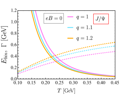
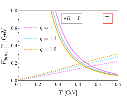
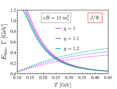
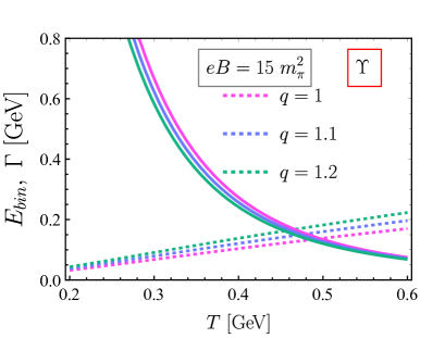
Figure 7: The binding energies (solid lines) and decay widths (dashed lines) for charmonium $J/\Psi$ (left panel) and bottomonium $\Upsilon$ (right panel) as a function of temperature at different values of the non-extensive parameter. In all plots, a fixed temperature of $T=0.3$ GeV and zero chemical potential are chosen. The upper and lower panels are the numerical results performed at zero magnetic field and finite magnetic field $eB=15~{}m_{\pi}^{2}$, respectively.

Based on the computations of the binding energies and decay widths for heavy quarkonia, we can estimate the melting temperatures $(T_{\rm melt})$ of heavy quarkonia, which are determined by a common criterion that the binding energy coincides with the decay width for a quarkonium state, i.e., $\Gamma(T_{\rm melt})=E_{bin}(T_{\rm melt})$ Mocsy:2007jz .

Now, let us delve into the impact of non-extensivity on the binding energies and decay widths of heavy quarkonia. In figure. 7, we depict the binding energies and decay widths for charmonium $J/\Psi$ (left panel) and bottomonium $\Upsilon$ (right panel) as functions of temperature, both in the absence and presence of a magnetic field. The solid lines represent binding energies of $J/\Psi$ and $\Upsilon$, whereas the dotted lines correspond to decay widths of $J/\Psi$ and $\Upsilon$, incorporating varying degrees of non-extensivity. We observe that binding energies of $J/\Psi$ and $\Upsilon$ decrease, whereas decay widths increase with increasing temperature. The binding energies of $J/\Psi$ and $\Upsilon$ in the magnetic field are slightly smaller than those in the pure thermal case. As shown in the upper panel of figure. 7, the non-extensive correction with $(q-1)>0$ reduces the binding energies of $J/\Psi$ and $\Upsilon$ due to an increase in the Debye mass and subsequently stronger screening of the QGP medium. As for decay widths of $J/\Psi$ and $\Upsilon$, the inclusion of non-extensivity amplifies their magnitude, which is inherited from the characteristics of the $\mathrm{Im}\,V$, as depicted in the left panel of figure. 6. We also observe that the decay widths of $J/\Psi$ and $\Upsilon$ are slightly decreased in a magnetic field compared to a purely thermal case, which holds for both the extensive and non-extensive QGP.

Magnetic field	State	$T_{\rm melt}^{q=1}$	$T_{\rm melt}^{q=1.1}$	$T_{\rm melt}^{q=1.2}$	Ref. Lafferty:2019jpr
$eB=0$	$J/\Psi$	0.254	0.232	0.219	0.267
$eB=15m_{\pi}^{2}$	$J/\Psi$	0.270	0.255	0.243
$eB=0$	$\Upsilon$	0.468	0.431	0.411	0.440
$eB=15m_{\pi}^{2}$	$\Upsilon$	0.496	0.472	0.453

Table 1: Melting temperatures of charmonium ($J/\Psi$) and bottomonium ($\Upsilon$) both in the absence and presence of a magnetic field for different values of $q$. The results at $q=1$ are compared with a recent work based on lattice QCD Lafferty:2019jpr .

In the figure. 7, the intersection points of solid and dashed lines of the same color denote the melting temperatures of heavy quarkonia. The melting temperatures of $J/\Psi$ and $\Upsilon$ for different values of $q$ in both the absence and presence of a magnetic field are summarized in Table 1. In the absence of non-extensivity, our computed melting temperatures align reasonably well with lattice data. The table reveals that although the magnetic field may induce a moderate increase in melting temperatures, thereby delaying the dissociation of heavy quarkonia, the incorporation of non-extensivity markedly accelerates the dissociation processes of heavy quarkonia can be significantly accelerated, leading to an earlier onset of dissociation. Furthermore, the decreasing trend of melting temperatures for $J/\Psi$ and $\Upsilon$ with varying $q$ is almost unaffected by the magnetic field.

6 Summary

In this paper, we incorporated the concept of non-extensivity into the HTL resummed perturbative theory, utilizing the non-extensive statistical mechanics parameterized by a non-extensive parameter $q$. Utilizing the real-time formalism, we systematically investigated the non-extensive corrections to the retarded, advanced, and symmetric (time-ordered) HTL gluon self-energies, as well as the resulting resummed gluon propagators, both in the absence and presence of a magnetic field. In the massless limit and without a magnetic field, we found that the incorporation of non-extensivity leads to distinct shifts in the retarded/advanced and symmetric Debye masses. Specifically, in the leading order of $(q-1)$, the retarded/advanced Debye mass at zero chemical potential is modified from $\frac{g^{2}T^{2}}{6}(2N_{c}+N_{f})$ to:

$$\frac{g^{2}T^{2}}{6}2N_{c}\left[1+\left(q-1\right)\left(\frac{18\zeta(3)}{\pi^{2}}-2\right)\right]+\frac{g^{2}T^{2}}{6}N_{f}\left[1+\left(q-1\right)\left(\frac{27\zeta(3)}{\pi^{2}}-2\right)\right],$$

while the symmetric Debye mass is modified to:

$$\frac{g^{2}T^{2}}{6}2N_{c}\left[1+\left(q-1\right)\left(\frac{36\zeta(3)}{\pi^{2}}-3\right)\right]+\frac{g^{2}T^{2}}{6}N_{f}\left[1+\left(q-1\right)\left(\frac{54\zeta(3)}{\pi^{2}}-3\right)\right].\\$$

When a magnetic field is considered, the Landau quantization of light quark motions leads to distinct forms of the Debye masses in the one-loop contributions from quarks and gluons to the retarded/advanced HTL gluon self-energies, necessitating a clear distinction between them. We observed that the retarded Debye mass becomes slightly larger in a finite magnetic field than in a zero magnetic field. When non-extensivity of the system is taken into account, the slope of retarded Debye mass with respect to $q$ for a zero magnetic field becomes steeper than that for a finite magnetic field. Consequently, the retarded Debye mass enhances more significantly as $q$ increases in the absence of a magnetic field, occasionally even exceeding the value observed in the presence of a magnetic field.

Applying non-extensive modified resummed gluon propagators, we obtained the dielectric permittivity, which encapsulates the properties of the QGP medium. Subsequently, this permittivity was employed to compute the complex heavy quark potential. Our observations revealed that the real part of the potential at $q=1$ exhibits a slight flattening in the presence of a magnetic field compared to the scenario without a magnetic field. When accounting for non-extensivity, the real part of the potential decreases with increasing $q$ at a fixed separation distance. Notably, the slope of the real part of the potential with respect to $q$ in the absence of a magnetic field is steeper than that observed in the presence of a magnetic field. Consequently, the difference between the real part of the potential in the two scenarios initially diminishes but subsequently increases. Ultimately, for $q$ values exceeding 1.2, the real part of the potential in the presence of a magnetic field surpasses that in the absence of a magnetic field. Incorporating non-extensivity enhances the magnitude of the imaginary part of the potential, whereas the presence of a magnetic field reduces it. Notably, the imaginary part of the potential arising from the quark contribution to the gluon self-energy exhibits significant anisotropy in a magnetic field, although this anisotropy is largely mitigated by the dominant contribution of $\mathrm{Im}\,V^{\rm gluon}$.

Using the obtained real part of the potential, we solved the time-independent Schr$\ddot{\rm o}$dinger equation for the radial wave function to determine the binding energies of heavy quarkonia, specifically $J/\Psi$ and $\Upsilon$. Additionally, performing the coordinate space integration and folding with probability density and imaginary part of the potential, we calculated the decay widths of heavy quarkonia. Inheriting traits from heavy quark potential, the binding energies of $J/\Psi$ and $\Upsilon$ decrease, while their decay widths increase with rising temperature and $q$. Subsequently, we estimated the melting temperatures of heavy quarkonia. Our findings indicated that the melting temperatures decrease as $q$ increases, leading to earlier dissociation of heavy quarkonia. Conversely, the presence of a magnetic field results in a slight increase in the melting temperatures, thereby delaying the dissociation process of heavy quarkonia.

Appendix A Non-extensive gluon self-energy in the zero magnetic field

Utilizing eq. (11) and eq. (30), as well as applying the Feynman rule, the one-loop contribution from quarks to the retarded gluon polarization tensor depicted in figure. 8 can read as

$$\Pi^{\mu\nu,\rm quark}_{R}(Q)= -iN_{f}g^{2}\int\frac{d^{4}K}{(2\pi)^{4}}\big{\{}\mathrm{Tr}[t_{b}\gamma^{\mu}S_{11}(K)t_{a}\gamma^{\nu}S_{11}(P)]$$

$$- \mathrm{Tr}[t_{b}\gamma^{\mu}S_{21}(K)t_{a}\gamma^{\nu}S_{12}(P)]\big{\}}$$ (147)

$$= -iN_{f}\frac{g}{4}^{2}\int\frac{d^{4}K}{(2\pi)^{4}}4(K^{\mu}P^{\nu}+K^{\nu}P^{\mu}-g^{\mu\nu}K\cdot P)[\Delta_{F}(K)\Delta_{R}(P)$$

$$+ \Delta_{A}(K)\Delta_{F}(P)+\Delta_{R}(K)\Delta_{R}(P)+\Delta_{A}(K)\Delta_{A}(P)],$$ (148)

where $P=K+Q$, $t_{a,b}$ are the generators of color group, and $S_{ij}(K)\equiv\displaystyle{\not}K\Delta_{ij}(K)$. The minus sign in front of the second square bracket of eq. (147) appears due to the vertex of type-2 field Landsman:1986uw . In deriving eq. (148) from eq. (147), we utilized the eq. (24) and eq. (25), and performed the trace over the gamma matrices as well as suppressed the color indices.

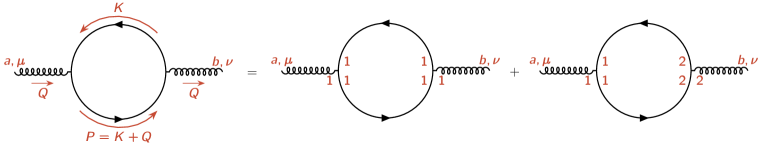
Figure 8: One-loop diagram for quark contribution to retarded gluon polarization tensor.

It should be noted that $\Delta_{R}(K)\Delta_{R}(P)$ and $\Delta_{A}(K)\Delta_{A}(P)$ in the integrand of eq. (148) are zero upon integration over $k_{0}$. Given our focus on the temporal component of the gluon self-energy, we set $\mu=\nu=0$ directly to obtain $(K^{\mu}P^{\nu}+K^{\nu}P^{\mu}-g^{\mu\nu}K\cdot P)=(k_{0}p_{0}+\bm{k}\cdot\bm{p})$. Consequently, the temporal component of $\Pi_{R}^{\mu\nu,\rm quark}(Q)$, denoted as $\Pi_{R}^{\rm quark}(Q)$ is expressed as

$$\Pi_{R}^{\rm quark}(Q)= -iN_{f}g^{2}\int\frac{d^{4}K}{(2\pi)^{4}}(k_{0}p_{0}+\bm{k}\cdot\bm{p})\left[{\Delta}_{F}(K){\Delta}_{R}(P)+{\Delta}_{A}(K){\Delta}_{F}(P)\right]$$ (149)

$$= -N_{f}g^{2}\int\frac{d^{4}K}{(2\pi)^{3}}(k_{0}p_{0}+\bm{k}\cdot\bm{p})\Bigg{[}\frac{1-2\Theta(k_{0})f_{q,F}^{+}(k_{0})-2\Theta(-k_{0})f_{q,F}^{-}(-k_{0})}{P^{2}+i\ \mathrm{sgn}(p_{0})\epsilon}$$

$$\times \delta(K^{2})+\frac{1-2\Theta(p_{0})f_{q,F}^{+}(p_{0})-2\Theta(-p_{0})f_{q,F}^{-}(-p_{0})}{K^{2}-i\ \mathrm{sgn}(k_{0})\epsilon}\delta(P^{2})\Bigg{]}$$ (150)

$$= 2N_{f}g^{2}\int\frac{d^{4}K}{(2\pi)^{3}}\bigg{\{}\Big{[}(\Theta(k_{0})\left(f_{q,F}^{+}(k_{0})+f_{q,F}^{-}(k_{0})\right)$$

$$+ \Theta(-k_{0})\left(f_{q,F}^{+}(-k_{0})+f_{q,F}^{-}(-k_{0})\right)\Big{]}\delta(k_{0}^{2}-\bm{k}^{2})$$

$$\times \frac{k_{0}(k_{0}+\omega)+\bm{k}\cdot(\bm{k}+\widetilde{\bm{q}})}{(k_{0}+\omega)^{2}-(\bm{k}+\widetilde{\bm{q}})^{2}+i\mathrm{sgn}(k_{0}+\omega)\epsilon}\bigg{\}}$$ (151)

$$= N_{f}g^{2}\int\frac{dkk^{2}d\Omega_{k}}{(2\pi)^{3}}\frac{1}{k}\left(f_{q,F}^{+}(k)+f_{q,F}^{-}(k)\right)$$

$$\times \bigg{[}\frac{k(k+\omega)+\bm{k}\cdot(\bm{k}+\widetilde{\bm{q}})}{(k+\omega)^{2}-(\bm{k}+\widetilde{\bm{q}})^{2}+i\epsilon}+\frac{-k(-k+\omega)+\bm{k}\cdot(\bm{k}+\widetilde{\bm{q}})}{(-k+\omega)^{2}-(\bm{k}+\widetilde{\bm{q}})^{2}-i\epsilon}\bigg{]}.$$ (152)

From eq. (150) to eq. (152), we have used the momentum substitution $K\to-P$ and $d\Omega_{k}=d\phi\sin\theta d\theta$. Here, the vacuum part has been neglected because it is suppressed compared to the medium part in the HTL approximation. Considering that $\omega/k$ and $\widetilde{q}/k$ in the HTL approximation are small terms, the square bracket in eq. (152) can be expanded as follows:

$$\frac{k(k+\omega)+\bm{k}\cdot(\bm{k}+\widetilde{\bm{q}})}{(k+\omega)^{2}-(\bm{k}+\widetilde{\bm{q}})^{2}+i\epsilon} =\frac{2k^{2}+k\omega+kq\cos\theta}{2k\omega+Q^{2}-2k\widetilde{q}\cos\theta+i\epsilon}$$ (153)

$$\simeq\frac{k}{\omega-\widetilde{q}\cos\theta+i\epsilon}-\frac{1}{2}\frac{Q^{2}}{(\omega-q\cos\theta+i\epsilon)^{2}}$$

$$+\frac{1}{2}\frac{\omega+\widetilde{q}\cos\theta}{\omega-\widetilde{q}\cos\theta+i\epsilon},$$ (154)

$$\frac{-k(-k+\omega)+\bm{k}\cdot(\bm{k}+\widetilde{\bm{q}})}{(-k+\omega)^{2}-(\bm{k}+\widetilde{\bm{q}})^{2}-i\epsilon} =\frac{2k^{2}-k\omega+k\widetilde{q}\cos\theta}{-2k\omega+Q^{2}-2k\widetilde{q}\cos\theta-i\epsilon}$$ (155)

$$\simeq-\frac{k}{\omega+\widetilde{q}\cos\theta+i\epsilon}-\frac{1}{2}\frac{Q^{2}}{(\omega+\widetilde{q}\cos\theta+i\epsilon)^{2}}$$

$$+\frac{1}{2}\frac{\omega-\widetilde{q}\cos\theta}{\omega+\widetilde{q}\cos\theta+i\epsilon},$$ (156)

where $x=\bm{k}\cdot\widetilde{\bm{q}}/(|\bm{k}||\widetilde{\bm{q}}|)=\cos\theta$. Since the first term in both eq. (154) and eq. (156) is an odd function of $x$, they integrate to zero over the range from $-1$ to 1. Therefore, eq. (152) simplifies to the following result:

$$\Pi_{R}^{\rm quark}(Q) =-N_{f}g^{2}\int\frac{k^{2}dkd\Omega_{k}}{2(2\pi)^{3}}\frac{1}{k}\left(f_{q,F}^{+}(k)+f_{q,F}^{-}(k)\right)$$

$$\times\left[\frac{1-x^{2}}{[x+(\omega+i\epsilon)/\widetilde{q}]^{2}}+\frac{1-x^{2}}{[-x+(\omega+i\epsilon)/\widetilde{q}]^{2}}\right].$$ (157)

By utilizing eq. (11) and eq. (32), the one-loop contribution from quarks to the symmetric gluon self-energy tensor is expressed as

$$\Pi^{\mu\nu,\rm quark}_{F}(Q)= -iN_{f}g^{2}\int\frac{d^{4}K}{(2\pi)^{4}}\big{\{}\mathrm{Tr}[t_{b}\gamma^{\mu}S_{11}(K)t_{a}\gamma^{\nu}S_{11}(P)]$$

$$+ \mathrm{Tr}[t_{b}\gamma^{\mu}S_{22}(K)t_{a}\gamma^{\nu}S_{22}(P)]\big{\}}$$ (158)

$$= -iN_{f}g^{2}\int\frac{d^{4}K}{(2\pi)^{4}}(K^{\mu}P^{\nu}+K^{\nu}P^{\mu}-g^{\mu\nu}K\cdot P)$$

$$\times [\Delta_{F}(K)\Delta_{F}(P)-(\Delta_{R}(K)-\Delta_{A}(K))(\Delta_{R}(P)-\Delta_{A}(P))].$$ (159)

Utilizing the relation $\Delta_{R}(K)-\Delta_{A}(K)=-i2\pi\delta(K^{2})\mathrm{sgn}(k_{0})$, and focusing specifically on the temporal component where $\mu=\nu=0$, we obtain

$$\Pi_{F}^{\rm quark}(Q) =iN_{f}g^{2}\int\frac{d^{4}K}{(2\pi)^{2}}(k_{0}p_{0}+\bm{k}\cdot\bm{p})\big{\{}[1-2\Theta(k_{0})f_{q,F}^{+}(k_{0})-2\Theta(-k_{0})f_{q,F}^{-}(-k_{0})]$$

$$\times[1-2\Theta(p_{0})f_{q,F}^{+}(p_{0})-2\Theta(-p_{0})f_{q,F}^{-}(-p_{0})]-\mathrm{sgn}(k_{0})\mathrm{sgn}(p_{0})\big{\}}$$

$$\times\delta(K^{2})\delta(P^{2})$$ (160)

$$=iN_{f}g^{2}\int\frac{k^{2}dkd\Omega_{k}}{(2\pi)^{2}}(k(k+\omega)+\bm{k}\cdot(\bm{k}+\widetilde{\bm{q}}))\frac{1}{2k}\delta(Q^{2}+2k\omega-2\bm{k}\cdot\widetilde{\bm{q}})$$

$$\times[-2f_{q,F}^{+}(k)-2f_{q,F}^{+}(k+\omega)+4f_{q,F}^{+}(k)f_{q,F}^{+}(k+\omega)]$$

$$+iN_{f}g^{2}\int\frac{dkk^{2}d\Omega_{k}}{(2\pi)^{2}}(-k(-k+\omega)+\bm{k}\cdot(\bm{k}+\widetilde{\bm{q}}))\frac{1}{2k}\delta(Q^{2}-2k\omega-2\bm{k}\cdot\widetilde{\bm{q}})$$

$$\times[-2f_{q,F}^{-}(k)-2f_{q,F}^{-}(k-\omega)+4f_{q,F}^{-}(k)f_{q,F}^{-}(k-\omega)].$$ (161)

In the HTL approximation with soft momentum limit $\omega/T\ll 1$, ${f}_{q,F}^{\pm}(k\pm\omega)$ can be expanded to the leading order of $\omega/T$, yields

$${f}_{q,F}^{\pm}(k\pm\omega)\approx{f}_{q,F}^{\pm}(k)\mp\frac{\omega q}{T}\exp_{q}\left(\frac{k\mp\mu}{T}\right)\left[{f}_{q,F}^{\pm}(k)\right]^{2}.$$ (162)

In eq. (161), $\delta(Q^{2}\pm 2k\omega-2\bm{k}\cdot\widetilde{\bm{q}})$ can be rewritten as $\frac{1}{2k\widetilde{q}}\delta(Q^{2}/(2k\widetilde{q})\pm\omega/\widetilde{q}-x)$, subsequently, the term $Q^{2}/(2k\widetilde{q})$ in the HTL approximation with $k\gg\omega$ becomes irrelevant and can be reasonably removed. Then, eq. (161) can be rewritten as

$$\Pi_{F}^{\rm quark}(Q)=-iN_{f}g^{2}\int\frac{dkk^{2}}{(2\pi)}\left[f_{q,F}^{+}(k)(1-f_{q,F}^{+}(k))+f_{q,F}^{-}(k)(1-f_{q,F}^{-}(k))\right]\frac{2}{\widetilde{q}}\Theta(\widetilde{q}^{2}-\omega^{2}),$$ (163)

where we have used the integral over the angle, yielding

$$\int d\Omega_{k}\delta(\omega/\widetilde{q}\pm x)=2\pi\Theta(\widetilde{q}^{2}-\omega^{2}).$$ (164)

Since we are interested in the space-like region within the static limit ($\omega\to 0$), which results in $\Theta(\widetilde{q}^{2}-\omega^{2})=1$.

The detailed derivation of the one-loop contribution from gluons to the gluon self-energy can be found in Refs. Wang:2022dcw ; Gorda:2023zwy ; Bellac:2011kqa . By repeating the computation procedure in Ref. Bellac:2011kqa and applying the non-extensive bare gluon propagators listed in eqs. (28) and (29), the gluonic contribution (including the gluon-loop, ghost-loop, and tadpole contributions) to the retarded gluon self-energy tensor is given as

$$\Pi_{R}^{\mu\nu,\rm gluon}(Q) =-i2N_{c}g^{2}\frac{d^{4}K}{(2\pi)^{4}}(K^{\mu}P^{\nu}+K^{\nu}P^{\mu}-g^{\mu\nu}K\cdot P)$$

$$\times[\tilde{\Delta}_{F}(K)\tilde{\Delta}_{R}(P)+\tilde{\Delta}_{A}(K)\tilde{\Delta}_{F}(P)].$$ (165)

Here, $G_{ij}(K)\equiv\tilde{\Delta}_{ij}(K)$. Using the HTL approximation and concerning the temporal component, a straightforward calculation leads to

$$\Pi_{R}^{\rm gluon}(Q) =2N_{c}g^{2}\int\frac{k^{2}dkd\Omega_{k}}{(2\pi)^{3}}\frac{f_{q,B}(k)}{2k}\bigg{[}\frac{1+x^{2}}{[x+(\omega+i\epsilon)/\widetilde{q}]^{2}}+\frac{1+x^{2}}{[-x+(\omega+i\epsilon)/\widetilde{q}]^{2}}\bigg{]}.$$ (166)

For the one-loop contribution from gluons to the symmetric gluon self-energy tensor, it can be expressed as

$$\Pi^{\mu\nu,\rm gluon}_{F}(Q)= -i2N_{c}g^{2}\int\frac{d^{4}K}{(2\pi)^{4}}(K^{\mu}P^{\nu}+K^{\nu}P^{\mu}-g^{\mu\nu}K\cdot P)$$

$$\times\left[\tilde{\Delta}_{F}(K)\tilde{\Delta}_{F}(P)-\left(\tilde{\Delta}_{R}(K)-\tilde{\Delta}_{A}(K)\right)\left(\tilde{\Delta}_{R}(P)-\tilde{\Delta}_{A}(P)\right)\right].$$ (167)

In the HTL approximation within the small $\omega$ limit, the temporal component of the above equation yields,

$$\Pi^{\rm gluon}_{F}(Q)=-i2N_{c}g^{2}\int\frac{dkk^{2}}{2\pi}f_{q,B}(k)(1+f_{q,B}(k))\frac{2}{\widetilde{q}}\Theta(\widetilde{q}^{2}-\omega^{2}),$$ (168)

which has the same structure as eq. (163) but with $f_{q,F}$ replaced by a non-extensive deformed Bose-Einstein distribution function.

Appendix B Non-extensive gluon self-energy in the finite magnetic field

Similar to the case of a zero magnetic field, the one-loop contribution from quarks to the retarded gluon self-energy tensor in the magnetic field is expressed as

$$\Pi^{\mu\nu,\rm quark}_{R,B}(Q)=-i\sum_{f}\sum_{n,l=0}\frac{g^{2}}{4}\int\frac{d^{2}K_{\|}}{(2\pi)^{2}}L^{\mu\nu}\left[\Delta^{n,f}_{F}(K)\Delta^{l,f}_{R}(P)+\Delta^{n,f}_{A}(K)\Delta^{l,f}_{F}(P)\right],$$ (169)

where $S_{R/A/F}^{n,f}(K)=\exp\left(-\frac{\bm{k}_{\perp}^{2}}{|e_{f}B|}\right)\sum_{n=0}^{\infty}(-1)^{n}D_{n}^{f}(k)\Delta_{R/A/F}^{n,f}(K)$ and the expression of tensor $L^{\mu\nu}$ is given as

$$L^{\mu\nu}=\int\frac{d^{2}\bm{k}_{\perp}}{(2\pi)^{2}}(-1)^{n+l}\exp\left(\frac{-\bm{k}_{\perp}^{2}-\bm{p}_{\perp}^{2}}{|e_{f}B|}\right)\mathrm{Tr}[\gamma^{\mu}D_{n}^{f}(K)\gamma^{\nu}D_{l}^{f}(P)]$$ (170)

In the HTL approximation with the hierarchy of scale of $\widetilde{q}^{2}\ll eB\sim T^{2}$, the tensor $L^{\mu\nu}$ can be further simplified to $L^{\mu\nu}=(-1)^{n+l}\frac{|e_{f}B|}{\pi}\big{[}4|e_{f}B|n\delta_{l-1}^{n-1}g_{\|}^{\mu\nu}+(\delta^{n}_{l}+\delta^{n-1}_{l-1})(K_{\|}^{\mu}P_{\|}^{\nu}+K_{\|}^{\nu}P_{\|}^{\mu}-g_{\|}^{\mu\nu}(K_{\|}\cdot P_{\|}))-(\delta_{l}^{n-1}+\delta^{n}_{l-1})(K_{\|}\cdot P_{\|})g_{\perp}^{\mu\nu}\big{]}$ Zhang:2023ked . The metric is defined as $g^{\mu\nu}=g^{\mu\nu}_{\|}+g_{\perp}^{\mu\nu}$, where $g^{\mu\nu}_{\|}=\mathrm{diag}(1,0,0,-1)$ and $\mathrm{diag}(0,-1,-1,0)$. In the soft momentum transfer limit, the perturbative QCD interaction cannot induce the Landau level transition for light (anti-)quarks, because they do not possess enough energy to jump across the energy gap separating the Landau levels, which is proportional to $\sqrt{eB}$. Consequently, by taking $n=l$, the tensor $L^{\mu\nu}$ resonantly simplifies to: $L^{\mu\nu}=\frac{e_{f}B}{\pi}\alpha_{0n}[2n|e_{f}B|g_{\|}^{\mu\nu}+(K_{\|}^{\mu}P_{\|}^{\nu}+K_{\|}^{\nu}P_{\|}^{\mu})-g_{\|}^{\mu\nu}(K_{\|}\cdot P_{\|})]$, where $\alpha_{0n}=(2-\delta_{0,n})$ is the Landau level-dependent spin degeneracy. Focusing solely on the temporal component of $\Pi^{\mu\nu,\rm quark}_{R,B}(Q)$, we arrive at the following result:

$$\Pi^{\rm quark}_{R,B}(Q)= -\sum_{f}\sum_{n=0}\frac{g^{2}}{4}\int\frac{d^{2}K_{\|}}{(2\pi)}\bigg{\{}\bigg{[}(1-2\Theta(k_{0})f_{q,F}^{+}(k_{0})-2\Theta(-k_{0})f_{q,F}^{-}(-k_{0}))$$

$$\times\frac{L^{00}(k_{0})\delta(K_{\|}^{2}-2n|e_{f}B|)}{P_{\|}^{2}-2n|e_{f}B|+i\,\mathrm{sgn}(p_{0})\epsilon}\bigg{]}+\bigg{[}(1-2\Theta(p_{0})f_{q,F}^{+}(p_{0})-2\Theta(-p_{0})f^{-}_{q,F}(-p_{0}))$$

$$\times\frac{L^{00}(k_{0})\delta(P_{\|}^{2}-2n|e_{f}B|)}{K_{\|}^{2}-2n|e_{f}B|-i\,\mathrm{sgn}(k_{0})\epsilon}\bigg{]}\bigg{\}}.$$ (171)

Here, $L^{00}(k_{0})=\alpha_{0n}(k_{0}p_{0}+k_{z}p_{z}+2n|e_{f}B|)\frac{|e_{f}B|}{\pi}$. In the presence of a magnetic field, it is essential to isolate the vacuum part and medium part in $\Pi^{\rm quark}_{R,B}(Q)$. In a magnetic field, the vacuum part in $\Pi^{\rm quark}_{R,B}(Q)$, denoted as $\Pi_{R,B,\rm vac}^{\rm quark}(Q)$, becomes significant, which has been extensively computed in the literature (see Refs. Fukushima:2015wck ; Hattori:2012ny ; Fukushima:2011nu , for details). It is given as:

$$\Pi_{R,B,\rm vac}^{\rm quark}(Q)=\frac{\widetilde{q}_{z}^{2}}{Q_{\|}^{2}}\sum_{f}\frac{\alpha_{s}|e_{f}B|}{\pi}-i\frac{\omega}{2}\sum_{f}\alpha_{s}|e_{f}B|\left[\delta(\omega-\widetilde{q}_{z})+\delta(\omega+\widetilde{q})\right],$$ (172)

where the form factor $\exp(-\frac{\bm{\widetilde{q}}_{\perp}^{2}}{2|e_{f}B|})$ has been removed in the HTL approximation with soft momentum limit $\widetilde{q}^{2}\ll T^{2}\sim eB$.

We proceed to the computation of medium part of $\Pi^{\rm quark}_{R,B}(Q)$, denoted as $\mathrm{Re}\,\Pi^{\mathrm{quark}}_{R,B,\rm med}$, which can be computed as follows:

$$\mathrm{Re}\,\Pi^{\rm quark}_{R,B,\rm med}(Q)= -\sum_{f}\sum_{n=0}\frac{g^{2}}{4}\int\frac{dk_{z}}{2\pi}\bigg{\{}\bigg{[}-\frac{f^{+}_{q,F}(E_{k_{z},n}^{f})}{E_{k_{z},n}^{f}}\frac{L^{00}(E_{k_{z},n}^{f})}{(\omega+E_{k_{z},n}^{f})^{2}-(E_{p_{z},n}^{f})^{2}}$$

$$- \frac{f^{-}_{q,F}(E_{k_{z},n}^{f})}{E_{k_{z},n}^{f}}\frac{L^{00}(-E_{k_{z},n}^{f})}{(\omega-E_{k_{z},n}^{f})^{2}-(E_{p_{z},n}^{f})^{2}}-\frac{f^{+}_{q,F}(E_{p_{z},n}^{f})}{E_{p_{z},n}^{f}}\frac{L^{00}(-\omega+E_{p_{z},n}^{f})}{(\omega+E_{p_{z},n}^{f})^{2}-(E_{k_{z},n}^{f})^{2}}$$

$$- \frac{f^{-}_{q,F}(E_{p_{z},n}^{f})}{E_{p_{z},n}^{f}}\frac{L^{00}(-\omega-E_{p_{z},n}^{f})}{(\omega+E_{p_{z},n}^{f})^{2}-(E_{k_{z},n}^{f})^{2}}\bigg{]}\bigg{\}},$$ (173)

where $L^{00}(\pm E^{f}_{k_{z},n})=2(E^{f}_{k_{z},n})^{2}\pm\omega E^{f}_{k_{z},n}+\widetilde{q}_{z}k_{z}$, and $L^{00}(-\omega\pm E^{f}_{p_{z},n})=(E^{f}_{p_{z},n})^{2}\mp\omega E^{f}_{p_{z},n}+(E^{f}_{k_{z},n})^{2}+k_{z}\widetilde{q}_{z}$. By taking the static limit ($\omega\to 0$), the above equation can be simplified as

$$\underset{\omega\to 0}{\mathrm{lim}}\mathrm{Re}\,\Pi^{\rm quark}_{R,B,\rm med}(Q)= -\sum_{f}\sum_{n=1}\frac{g^{2}|e_{f}B|}{4\pi}\int\frac{dk_{z}}{(2\pi)}\bigg{\{}-\frac{2(E^{f}_{k_{z},n})^{2}+\widetilde{q}_{z}k_{z}}{E_{k_{z},n}^{f}(E_{k_{z},n}^{f})^{2}-(E_{p_{z},n}^{f})^{2}}$$

$$\times \left[f^{+}_{q,F}(E_{k_{z},n}^{f})+f^{-}_{q,F}(E_{k_{z},n}^{f})\right]-\frac{(E^{f}_{p_{z},n})^{2}+(E^{f}_{k_{z},n})^{2}+\widetilde{q}_{z}k_{z}}{E_{p_{z},n}^{f}(E_{p_{z},n}^{f})^{2}-(E_{k_{z},n}^{f})^{2}}$$

$$\times \left[f^{+}_{q,F}(E_{p_{z},n}^{f})+f^{-}_{q,F}(E_{p_{z},n}^{f})\right]\bigg{\}}.$$ (174)

By extracting the imaginary part from eq. (B) and performing a momentum substitution $P\to-K$ in the first square bracket of eq. (B), we obtain:

$$\mathrm{Im}\,\Pi^{\rm quark}_{R,B,\rm med}(Q)= -\sum_{f}\sum_{n=0}^{\infty}\frac{g^{2}}{8}\int d^{2}K_{\|}L^{00}(k_{0})\delta(K_{\|}^{2}-2n|e_{f}B|)\delta(P_{\|}^{2}-2n|e_{f}B|)$$

$$\times \bigg{\{}\mathrm{sgn}(-k_{0})\left[\Theta(-p_{0})f^{+}_{q,F}(-p_{0})+\Theta(p_{0})f^{-}_{q,F}(p_{0})\right]$$

$$- \mathrm{sgn}(k_{0})\left[\Theta(p_{0})f^{+}_{q,F}(p_{0})+\Theta(-p_{0})f^{-}_{q,F}(-p_{0})\right]\bigg{\}}$$ (175)

$$= -\sum_{f}\sum_{n=0}^{\infty}\frac{g^{2}}{8}\int dk_{z}\frac{L^{00}(E_{k_{z},n}^{f})}{4E_{k_{z},n}^{f}E_{p_{z},n}^{f}}\left[-f^{-}_{q,F}(\omega+E_{k_{z},n}^{f})-f^{+}_{q,F}(\omega+E_{k_{z},n}^{f})\right]$$

$$\times \left[\delta(\omega+E_{k_{z},n}^{f}-E_{p_{z},n}^{f})+\delta(\omega+E_{k_{z},n}^{f}+E_{p_{z},n}^{f})\right]$$

$$- \sum_{f}\sum_{n=0}^{\infty}\frac{g^{2}}{8}\int dk_{z}\frac{L^{00}(-E_{k_{z},n}^{f})}{4E_{k_{z},n}^{f}E_{p_{z},n}^{f}}\left[f^{+}_{q,F}(E_{k_{z},n}^{f}-\omega)+f^{-}_{q,F}(E_{k_{z},n}^{f}-\omega)\right]$$

$$\times \left[\delta(\omega+E_{k_{z},n}^{f}-E_{p_{z},n}^{f})+\delta(\omega+E_{k_{z},n}^{f}+E_{p_{z},n}^{f})\right].$$ (176)

In eq. (176), only the delta functions related to the decay processes ($\delta(\omega+E^{f}_{k_{z},n}-E^{f}_{p_{z},n})$ and $\delta(\omega-E^{f}_{k_{z},n}+E^{f}_{p_{z},n})$) contribute to our work. Within the static limit ($\omega\to 0$), these delta functions of our interest can be explicitly worked out as

$$\delta(E_{k_{z},n}^{f}-E_{p_{z},n}^{f})=(E_{\widetilde{q}_{z}/2,n}^{f}/|\widetilde{q}_{z}|)\delta(k_{z}+\widetilde{q}_{z}/2).$$ (177)

By utilizing eq. (84) and performing the integration over $k_{z}$, eq. (176) in the static limit ($\omega\to 0$), finally can be computed as

$$\underset{\omega\to 0}{\mathrm{lim}}\frac{\mathrm{Im}\,\Pi^{\rm quark}_{R,B,\rm med}(Q)}{\omega}= -\sum_{f}\sum_{n=0}^{\infty}\frac{g^{2}}{4\pi}\frac{\alpha_{0n}2n|e_{f}B|^{2}}{E_{\widetilde{q}_{z}/2,n}^{f}|\widetilde{q}_{z}|}\frac{q}{2T}\bigg{[}\exp_{q}\left(\frac{E_{\widetilde{q}_{z}/2,n}^{f}+\mu}{T}\right)\left(f_{q,F}^{-}(E_{\widetilde{q}_{z}/2,n}^{f})\right)^{2}$$

$$+ \exp_{q}\left(\frac{E_{\widetilde{q}_{z}/2,n}^{f}-\mu}{T}\right)\left(f_{q,F}^{+}(E_{\widetilde{q}_{z}/2,n}^{f})\right)^{2}\bigg{]}.$$ (178)

Since we consider the massless QCD limit when light quarks occupy the lowest Landau level, $\mathrm{Im}\,\Pi_{R,B,\rm med}^{\rm quark}(Q)$ becomes zero.

The one-loop contribution from quarks to the symmetric gluon self-energy tensor in a magnetic field, denoted as $\Pi^{\mu\nu,\rm quark}_{F,B}(Q)$, is purely imaginary and can be expressed as

$$\Pi^{\mu\nu,\rm quark}_{F,B}(Q)= -i\sum_{f}\sum_{n,l}^{\infty}\frac{g^{2}}{4}\int\frac{d^{2}K_{\|}}{(2\pi)^{4}}L^{\mu\nu}\big{[}\Delta_{F}^{n,f}(K)\Delta_{F}^{l,f}(P)$$

$$- \left(\Delta_{R}^{n,f}(K)-\Delta_{A}^{n,f}(K)\right)\left(\Delta_{R}^{l,f}(P)-\Delta_{A}^{l,f}(P)\right)\big{]}.$$ (179)

By inserting the definite expressions of $\Delta_{R/A}^{n,f}(K)$ and $\Delta_{F}^{n,f}(K)$ into the above equation, and following a similar calculation procedure as for $\Pi^{\mu\nu,\rm quark}_{R,B}$, the temporal component of eq. (B) in the HTL approximation is computed as:

$$\Pi^{\rm quark}_{F,B}(Q)= i\sum_{f}\sum_{n=0}^{\infty}\frac{g^{2}}{4}\int d^{2}K_{\|}L^{00}(k_{0})\bigg{\{}\left[1-2\Theta(k_{0})f_{q,F}^{+}(k_{0})-2\Theta(-k_{0})f_{q,F}^{-}(-k_{0})\right]$$

$$\times \left[1-2\Theta(p_{0})f_{q,F}^{+}(p_{0})-2\Theta(-p_{0})f_{q,F}^{-}(-p_{0})\right]-\mathrm{sgn}(p_{0})\mathrm{sgn}(k_{0})\bigg{\}}$$

$$\times \delta(K_{\|}^{2}-2n|e_{f}B|)\delta(P_{\|}^{2}-2n|e_{f}B|).$$ (180)

By performing integration over $k_{0}$ and using the identities for Dirac delta functions, the above equation can be further computed as

$$\Pi^{\rm quark}_{F,B}(Q)= -i\sum_{f}\sum_{n=0}^{\infty}\frac{g^{2}}{4}\int\frac{dk_{z}}{4E_{k_{z},n}^{f}E_{p_{z},n}^{f}}\bigg{\{}L^{00}(E_{k_{z},n}^{f})\bigg{[}2f_{q,F}^{+}(E_{k_{z},n}^{f})+2f_{q,F}^{+}(\omega+E_{k_{z},n}^{f})$$

$$-4f_{q,F}^{+}(E_{k_{z},n}^{f})f_{q,F}^{+}(\omega+E_{k_{z},n}^{f})\bigg{]}$$

$$+L^{00}(-E_{k_{z},n}^{f})\bigg{[}2f_{q,F}^{-}(E_{k_{z},n}^{f})+2f_{q,F}^{-}(-\omega+E_{k_{z},n}^{f})$$

$$-4f_{q,F}^{-}(E_{k_{z},n}^{f})f_{q,F}^{-}(-\omega+E_{k_{z},n}^{f})\bigg{]}\bigg{\}}$$

$$\times\left[\delta(\omega+E_{k_{z},n}^{f}-E_{p_{z},n}^{f})+\delta(\omega+E_{k_{z},n}^{f}+E_{p_{z},n}^{f})\right].$$ (181)

By utilizing eq. (84) again and considering the decay processes, the above equation in the static limit ($\omega\to 0$) can finally be obtained as

$$\underset{\omega\to 0}{\mathrm{lim}}\Pi^{\rm quark}_{F,B}(Q)= -i\sum_{f}\sum_{n=0}^{\infty}\frac{g^{2}}{4\pi}\frac{\alpha_{n0}4n|e_{f}B|^{2}}{E_{\widetilde{q}_{z}/2,n}^{f}|\widetilde{q}_{z}|}\bigg{\{}\bigg{[}f_{q,F}^{+}(E_{\widetilde{q}_{z}/2,n}^{f})\left(1-f_{q,F}^{+}(E_{\widetilde{q}_{z}/2,n}^{f})\right)$$

$$+ f_{q,F}^{-}(E_{\widetilde{q}_{z}/2,n}^{f})\left(1-f_{q,F}^{-}(E_{\widetilde{q}_{z}/2,n}^{f})\right)\bigg{]}\bigg{\}}.$$ (182)

Since thermal gluons are not directly coupled to the magnetic field, the gluonic contribution to the symmetric HTL gluon self-energy in a magnetic field is consistent with that in the absence of a magnetic field, as presented in eq. (168).

References

• (1) J. Adams et al. [STAR], Nucl. Phys. A 757, 102-183 (2005) doi:10.1016/j.nuclphysa.2005.03.085 [arXiv:nucl-ex/0501009 [nucl-ex]].
• (2) K. Adcox et al. [PHENIX], Nucl. Phys. A 757, 184-283 (2005) doi:10.1016/j.nuclphysa.2005.03.086 [arXiv:nucl-ex/0410003 [nucl-ex]].
• (3) W. T. Deng and X. G. Huang, Phys. Rev. C 85, 044907 (2012) doi:10.1103/PhysRevC.85.044907 [arXiv:1201.5108 [nucl-th]].
• (4) V. Skokov, A. Y. Illarionov and V. Toneev, Int. J. Mod. Phys. A 24, 5925-5932 (2009) doi:10.1142/S0217751X09047570 [arXiv:0907.1396 [nucl-th]].
• (5) V. Voronyuk, V. D. Toneev, W. Cassing, E. L. Bratkovskaya, V. P. Konchakovski and S. A. Voloshin, Phys. Rev. C 83, 054911 (2011) doi:10.1103/PhysRevC.83.054911 [arXiv:1103.4239 [nucl-th]].
• (6) T. Toimela, Int. J. Theor. Phys. 24, 901 (1985) [erratum: Int. J. Theor. Phys. 26, 1021 (1987)] doi:10.1007/BF00671334
• (7) J. O. Andersen, L. E. Leganger, M. Strickland and N. Su, JHEP 08, 053 (2011) doi:10.1007/JHEP08(2011)053 [arXiv:1103.2528 [hep-ph]].
• (8) N. Haque, A. Bandyopadhyay, J. O. Andersen, M. G. Mustafa, M. Strickland and N. Su, JHEP 05, 027 (2014) doi:10.1007/JHEP05(2014)027 [arXiv:1402.6907 [hep-ph]].
• (9) J.I. Kapusta, Finite-Temperature Field Theory (Cambridge University Press, Cambridge, 1989).
• (10) M. Le Bellac, Thermal Field Theory (Cambridge University Press, Cambridge 1996).
• (11) H. A. Weldon, Phys. Rev. D 26, 1394 (1982) doi:10.1103/PhysRevD.26.1394.
• (12) J. Frenkel and J. C. Taylor, Nucl. Phys. B 334, 199-216 (1990) doi:10.1016/0550-3213(90)90661-V.
• (13) P. Elmfors, Nucl. Phys. B 487, 207-230 (1997) doi:10.1016/S0550-3213(96)00666-9 [arXiv:hep-ph/9608271 [hep-ph]].
• (14) E. Braaten and R. D. Pisarski, Phys. Rev. D 45, no.6, R1827 (1992) doi:10.1103/PhysRevD.45.R1827.
• (15) M. H. Thoma, [arXiv:hep-ph/0010164 [hep-ph]].
• (16) R. D. Pisarski, Nucl. Phys. A 525, 175-188 (1991) doi:10.1016/0375-9474(91)90325-Z.
• (17) S. Mrowczynski and M. H. Thoma, Phys. Rev. D 62, 036011 (2000) doi:10.1103/PhysRevD.62.036011 [arXiv:hep-ph/0001164 [hep-ph]].
• (18) M. H. Thoma, doi:10.1142/9789812830661_0002 [arXiv:hep-ph/9503400 [hep-ph]].
• (19) M. Laine, O. Philipsen, P. Romatschke and M. Tassler, JHEP 03, 054 (2007) doi:10.1088/1126-6708/2007/03/054 [arXiv:hep-ph/0611300 [hep-ph]].
• (20) M. Laine, JHEP 05, 028 (2007) doi:10.1088/1126-6708/2007/05/028 [arXiv:0704.1720 [hep-ph]].
• (21) Y. Burnier and A. Rothkopf, Phys. Lett. B 753, 232-236 (2016) doi:10.1016/j.physletb.2015.12.031 [arXiv:1506.08684 [hep-ph]].
• (22) A. Beraudo, J. P. Blaizot and C. Ratti, Nucl. Phys. A 806, 312-338 (2008) doi:10.1016/j.nuclphysa.2008.03.001 [arXiv:0712.4394 [nucl-th]].
• (23) H. X. Zhang and E. Wang, Phys. Rev. D 109, no.7, 074034 (2024) doi:10.1103/PhysRevD.109.074034 [arXiv:2301.09110 [hep-ph]].
• (24) G. D. Moore and D. Teaney, Phys. Rev. C 71, 064904 (2005) doi:10.1103/PhysRevC.71.064904 [arXiv:hep-ph/0412346 [hep-ph]].
• (25) S. Caron-Huot and G. D. Moore, Phys. Rev. Lett. 100, 052301 (2008) doi:10.1103/PhysRevLett.100.052301 [arXiv:0708.4232 [hep-ph]].
• (26) K. Fukushima, K. Hattori, H. U. Yee and Y. Yin, Phys. Rev. D 93, no.7, 074028 (2016) doi:10.1103/PhysRevD.93.074028 [arXiv:1512.03689 [hep-ph]].
• (27) E. Braaten, R. D. Pisarski and T. C. Yuan, Phys. Rev. Lett. 64, 2242 (1990) doi:10.1103/PhysRevLett.64.2242.
• (28) S. M. H. Wong, Z. Phys. C 53, 465-478 (1992) doi:10.1007/BF01625907.
• (29) Y. Burnier, M. Laine and M. Vepsalainen, JHEP 01, 043 (2008) doi:10.1088/1126-6708/2008/01/043 [arXiv:0711.1743 [hep-ph]].
• (30) M. H. Thoma and M. Gyulassy, Nucl. Phys. B 351, 491-506 (1991) doi:10.1016/S0550-3213(05)80031-8.
• (31) P. Romatschke and M. Strickland, Phys. Rev. D 68, 036004 (2003) doi:10.1103/PhysRevD.68.036004 [arXiv:hep-ph/0304092 [hep-ph]].
• (32) P. Romatschke and M. Strickland, Phys. Rev. D 70, 116006 (2004) doi:10.1103/PhysRevD.70.116006 [arXiv:hep-ph/0406188 [hep-ph]].
• (33) B. S. Kasmaei and M. Strickland, Phys. Rev. D 97, no.5, 054022 (2018) doi:10.1103/PhysRevD.97.054022 [arXiv:1801.00863 [hep-ph]].
• (34) Q. Du, A. Dumitru, Y. Guo and M. Strickland, JHEP 01, 123 (2017) doi:10.1007/JHEP01(2017)123 [arXiv:1611.08379 [hep-ph]].
• (35) A. Dumitru, Y. Guo and M. Strickland, Phys. Rev. D 79, 114003 (2009) doi:10.1103/PhysRevD.79.114003 [arXiv:0903.4703 [hep-ph]].
• (36) L. Dong, Y. Guo, A. Islam, A. Rothkopf and M. Strickland, JHEP 09, 200 (2022) doi:10.1007/JHEP09(2022)200 [arXiv:2205.10349 [hep-ph]].
• (37) A. Dumitru, Y. Guo, A. Mocsy and M. Strickland, Phys. Rev. D 79, 054019 (2009) doi:10.1103/PhysRevD.79.054019 [arXiv:0901.1998 [hep-ph]].
• (38) L. Thakur and Y. Hirono, JHEP 02, 207 (2022) doi:10.1007/JHEP02(2022)207 [arXiv:2111.08225 [hep-ph]].
• (39) L. Thakur, N. Haque and Y. Hirono, JHEP 06, 071 (2020) doi:10.1007/JHEP06(2020)071 [arXiv:2004.03426 [hep-ph]].
• (40) L. Thakur, N. Haque, U. Kakade and B. K. Patra, Phys. Rev. D 88, no.5, 054022 (2013) doi:10.1103/PhysRevD.88.054022 [arXiv:1212.2803 [hep-ph]].
• (41) C. Tsallis, J. Statist. Phys. 52, 479-487 (1988) doi:10.1007/BF01016429.
• (42) G. Wilk and Z. Wlodarczyk, Phys. Rev. Lett. 84, 2770 (2000) doi:10.1103/PhysRevLett.84.2770 [arXiv:hep-ph/9908459 [hep-ph]].
• (43) P. Huovinen and H. Petersen, Eur. Phys. J. A 48, 171 (2012) doi:10.1140/epja/i2012-12171-9 [arXiv:1206.3371 [nucl-th]].
• (44) K. Aamodt et al. [ALICE], Phys. Lett. B 693, 53-68 (2010) doi:10.1016/j.physletb.2010.08.026 [arXiv:1007.0719 [hep-ex]].
• (45) A. Adare et al. [PHENIX], Phys. Rev. D 83, 052004 (2011) doi:10.1103/PhysRevD.83.052004 [arXiv:1005.3674 [hep-ex]].
• (46) J. Chen, J. Deng, Z. Tang, Z. Xu and L. Yi, Phys. Rev. C 104, no.3, 034901 (2021) doi:10.1103/PhysRevC.104.034901 [arXiv:2012.02986 [nucl-th]].
• (47) Y. Su, Y. Sun, Y. Zhang and X. Chen, Nucl. Sci. Tech. 32, no.10, 108 (2021) doi:10.1007/s41365-021-00945-4 [arXiv:2109.14386 [hep-ex]].
• (48) C. Y. Wong and G. Wilk, Phys. Rev. D 87, no.11, 114007 (2013) doi:10.1103/PhysRevD.87.114007 [arXiv:1305.2627 [hep-ph]].
• (49) G. Che, J. Gu, W. Zhang and H. Zheng, J. Phys. G 48, no.9, 095103 (2021) doi:10.1088/1361-6471/ac09dc [arXiv:2010.14880 [nucl-th]].
• (50) M. Shao, L. Yi, Z. Tang, H. Chen, C. Li and Z. Xu, J. Phys. G 37, 085104 (2010) doi:10.1088/0954-3899/37/8/085104 [arXiv:0912.0993 [nucl-ex]].
• (51) Z. Tang, Y. Xu, L. Ruan, G. van Buren, F. Wang and Z. Xu, Phys. Rev. C 79, 051901 (2009) doi:10.1103/PhysRevC.79.051901 [arXiv:0812.1609 [nucl-ex]].
• (52) W. M. Alberico, A. Lavagno and P. Quarati, Eur. Phys. J. C 12, 499-506 (2000) doi:10.1007/s100529900220 [arXiv:nucl-th/9902070 [nucl-th]].
• (53) S. Sharma and M. Kaur, Phys. Rev. D 98, no.3, 034008 (2018) doi:10.1103/PhysRevD.98.034008 [arXiv:1802.05587 [hep-ph]].
• (54) T. Osada and G. Wilk, Phys. Rev. C 77, 044903 (2008) [erratum: Phys. Rev. C 78, 069903 (2008)] doi:10.1103/PhysRevC.77.044903 [arXiv:0710.1905 [nucl-th]].
• (55) M. Alqahtani, N. Demir and M. Strickland, Eur. Phys. J. C 82, no.10, 973 (2022) doi:10.1140/epjc/s10052-022-10943-4 [arXiv:2203.14968 [nucl-th]].
• (56) T. S. Biro and E. Molnar, Phys. Rev. C 85, 024905 (2012) doi:10.1103/PhysRevC.85.024905 [arXiv:1109.2482 [nucl-th]].
• (57) G. Gervino, A. Lavagno and D. Pigato, Central Eur. J. Phys. 10, 594-601 (2012) doi:10.2478/s11534-011-0123-3 [arXiv:1202.3091 [nucl-th]].
• (58) W. H. Wu, J. Q. Tao, H. Zheng, W. C. Zhang, X. Q. Liu, L. L. Zhu and A. Bonasera, Nucl. Sci. Tech. 34, no.10, 151 (2023) doi:10.1007/s41365-023-01307-y.
• (59) K. Kyan and A. Monnai, Phys. Rev. D 106, no.5, 054004 (2022) doi:10.1103/PhysRevD.106.054004 [arXiv:2205.01742 [nucl-th]].
• (60) T. Bhattacharyya, J. Cleymans and S. Mogliacci, Phys. Rev. D 94, 094026 (2016) doi:10.1103/PhysRevD.94.094026 [arXiv:1608.08965 [cond-mat.stat-mech]].
• (61) S. K. Tiwari, S. Tripathy, R. Sahoo and N. Kakati, Eur. Phys. J. C 78, no.11, 938 (2018) doi:10.1140/epjc/s10052-018-6411-y [arXiv:1709.06352 [hep-ph]].
• (62) R. Rath, S. Tripathy, B. Chatterjee, R. Sahoo, S. Kumar Tiwari and A. Nath, Eur. Phys. J. A 55, no.8, 125 (2019) doi:10.1140/epja/i2019-12814-3 [arXiv:1902.07922 [hep-ph]].
• (63) J. Rozynek and G. Wilk, J. Phys. G 36, 125108 (2009) doi:10.1088/0954-3899/36/12/125108 [arXiv:0905.3408 [nucl-th]].
• (64) A. Lavagno, D. Pigato and P. Quarati, J. Phys. G 37, no.11, 115102 (2010) doi:10.1088/0954-3899/37/11/115102 [arXiv:1005.4643 [nucl-th]].
• (65) Y. P. Zhao, S. Y. Zuo, C. M. Li, QCD chiral phase transition and critical exponents within the nonextensive Polyakov-Nambu-Jona-Lasinio model. Chin. Phys. C 45, 073105 (2021). doi:10.1088/1674-1137/abf8a2 [arXiv:2008.09276 [hep-ph]].
• (66) H. Hasegawa, Phys. Rev. E 80, 011126 (2009) doi:10.1103/PhysRevE.80.011126 [arXiv:0904.2399 [cond-mat.stat-mech]].
• (67) M. Rahaman, T. Bhattacharyya and J. e. Alam, [arXiv:1906.02893 [hep-ph]].
• (68) W. M. Alberico and A. Lavagno, Eur. Phys. J. A 40, 313-323 (2009) doi:10.1140/epja/i2009-10809-3 [arXiv:0901.4952 [nucl-th]].
• (69) A. Lavagno, Phys. Lett. A 301, 13-18 (2002) doi:10.1016/S0375-9601(02)00964-7 [arXiv:cond-mat/0207353 [cond-mat.stat-mech]
• (70) M. Biyajima, M. Kaneyama, T. Mizoguchi and G. Wilk, Eur. Phys. J. C 40, 243-250 (2005) doi:10.1140/epjc/s2005-02140-2 [arXiv:hep-ph/0403063 [hep-ph]].
• (71) M. Biyajima, T. Mizoguchi, N. Nakajima, N. Suzuki and G. Wilk, Eur. Phys. J. C 48, 597-603 (2006) doi:10.1140/epjc/s10052-006-0026-4 [arXiv:hep-ph/0602120 [hep-ph]].
• (72) M. Rahaman, T. Bhattacharyya and J. e. Alam, Int. J. Mod. Phys. A 36, no.20, 2150154 (2021) doi:10.1142/S0217751X21501542.
• (73) K. c. Chou, Z. b. Su, B. l. Hao and L. Yu, Phys. Rept. 118, 1-131 (1985) doi:10.1016/0370-1573(85)90136-X.
• (74) L. V. Keldysh, Zh. Eksp. Teor. Fiz. 47, 1515-1527 (1964).
• (75) M. E. Carrington and U. W. Heinz, Eur. Phys. J. C 1, 619-625 (1998) doi:10.1007/s100520050110 [arXiv:hep-th/9606055 [hep-th]].
• (76) M. Kurian, S. K. Das and V. Chandra, Phys. Rev. D 100, no.7, 074003 (2019) doi:10.1103/PhysRevD.100.074003 [arXiv:1907.09556 [nucl-th]].
• (77) E. Eichten, K. Gottfried, T. Kinoshita, J. B. Kogut, K. D. Lane and T. M. Yan, Phys. Rev. Lett. 34, 369-372 (1975) [erratum: Phys. Rev. Lett. 36, 1276 (1976)] doi:10.1103/PhysRevLett.34.369.
• (78) T. Matsui and H. Satz, Phys. Lett. B 178, 416-422 (1986) doi:10.1016/0370-2693(86)91404-8.
• (79) S. Jacobs, M. G. Olsson and C. Suchyta, III, Phys. Rev. D 33, 3338 (1986) [erratum: Phys. Rev. D 34, 3536 (1986)] doi:10.1103/PhysRevD.33.3338.
• (80) V. Agotiya, V. Chandra and B. K. Patra, Phys. Rev. C 80, 025210 (2009) doi:10.1103/PhysRevC.80.025210 [arXiv:0808.2699 [hep-ph]].
• (81) L. Thakur, N. Haque and H. Mishra, Phys. Rev. D 95, no.3, 036014 (2017) doi:10.1103/PhysRevD.95.036014 [arXiv:1611.04568 [hep-ph]].
• (82) L. Thakur, U. Kakade and B. K. Patra, Phys. Rev. D 89, no.9, 094020 (2014) doi:10.1103/PhysRevD.89.094020 [arXiv:1401.0172 [hep-ph]].
• (83) H. Satz, J. Phys. G 32, R25 (2006) doi:10.1088/0954-3899/32/3/R01 [arXiv:hep-ph/0512217 [hep-ph]].
• (84) A. Ayala, C. A. Dominguez, S. Hernandez-Ortiz, L. A. Hernandez, M. Loewe, D. Manreza Paret and R. Zamora, Phys. Rev. D 98, no.3, 031501 (2018) doi:10.1103/PhysRevD.98.031501 [arXiv:1805.08198 [hep-ph]].
• (85) A. Bazavov, N. Brambilla, X. Garcia Tormo, i, P. Petreczky, J. Soto and A. Vairo, Phys. Rev. D 86, 114031 (2012) doi:10.1103/PhysRevD.86.114031 [arXiv:1205.6155 [hep-ph]].
• (86) N. Brambilla, M. A. Escobedo, J. Ghiglieri and A. Vairo, JHEP 12, 116 (2011) doi:10.1007/JHEP12(2011)116 [arXiv:1109.5826 [hep-ph]].
• (87) M. Y. Jamal, I. Nilima, V. Chandra and V. K. Agotiya, Phys. Rev. D 97, no.9, 094033 (2018) doi:10.1103/PhysRevD.97.094033 [arXiv:1805.04763 [nucl-th]].
• (88) D. Lafferty and A. Rothkopf, Phys. Rev. D 101, no.5, 056010 (2020) doi:10.1103/PhysRevD.101.056010 [arXiv:1906.00035 [hep-ph]].
• (89) A. Mocsy and P. Petreczky, Phys. Rev. Lett. 99, 211602 (2007) doi:10.1103/PhysRevLett.99.211602 [arXiv:0706.2183 [hep-ph]].
• (90) N. P. Landsman and C. G. van Weert, Phys. Rept. 145, 141 (1987) doi:10.1016/0370-1573(87)90121-9.
• (91) Y. Wang, Q. Du and Y. Guo, Phys. Rev. D 106, no.5, 054033 (2022). doi:10.1103/PhysRevD.106.054033 [arXiv:2207.06039 [hep-ph]].
• (92) T. Gorda, R. Paatelainen, S. Säppi and K. Seppänen, JHEP 08, 021 (2023). doi:10.1007/JHEP08(2023)021 [arXiv:2304.09187 [hep-ph]].
• (93) M. L. Bellac, Cambridge University Press, 2011, ISBN 978-0-511-88506-8, 978-0-521-65477-7 doi:10.1017/CBO9780511721700.
• (94) K. Hattori and K. Itakura, Annals Phys. 334, 58-82 (2013) doi:10.1016/j.aop.2013.03.016 [arXiv:1212.1897 [hep-ph]].
• (95) K. Fukushima, Phys. Rev. D 83, 111501 (2011) doi:10.1103/PhysRevD.83.111501 [arXiv:1103.4430 [hep-ph]].