Upper and lower bounds on the subgeometric convergence of adaptive Markov chain Monte Carlo

Abstract

We investigate lower bounds on the subgeometric convergence of adaptive Markov chain Monte Carlo under any adaptation strategy. In particular, we prove general lower bounds in total variation and on the weak convergence rate under general adaptation plans. If the adaptation diminishes sufficiently fast, we also develop comparable convergence rate upper bounds that are capable of approximately matching the convergence rate in the subgeometric lower bound. These results provide insight into the optimal design of adaptation strategies and also limitations on the convergence behavior of adaptive Markov chain Monte Carlo. Applications to an adaptive unadjusted Langevin algorithm as well as adaptive Metropolis-Hastings with independent proposals and random-walk proposals are explored.

MSC: 60J05; 60J22; 60G07

Keywords: adaptive Metropolis-Hastings; lower bounds for adaptive MCMC; weak convergence of adaptive MCMC;

1 Introduction

Let $\pi$ be a Borel probability measure on a Polish space $\mathcal{X}$. Adaptive Markov chain Monte Carlo [Haario et al., 2001, Roberts and Rosenthal, 2007] is a widely successful framework to simulate realizations from $\pi$ when optimal tuning parameters for the Markov chain are not readily available. The adaptive process $(\Gamma_{t},X_{t})_{t=1}^{\infty}$ is constructed from a family of Markov kernels indexed by a set of potential tuning parameters. The discrete-time adaptive process first updates the tuning parameter $\Gamma_{t}|(\Gamma_{s},X_{s})_{0\leq s\leq t-1}$ with an adaptation strategy utilizing previous history and next, updates $X_{t}|\Gamma_{t},X_{t-1}$ using a Markov transition kernel. The goal is for the adaptive process to “learn” optimal tuning parameters so that the marginal distribution of the random variable $X_{t}$ produces a close approximation to the measure $\pi$.

With a large option for adaptation strategies, theoretical convergence rates of adaptive algorithms are less understood than for non-adaptive Markov chain Monte Carlo (MCMC) where fixed tuning parameters are chosen carefully beforehand. In particular, a theoretical understanding of the rate of convergence is essential in applications as it helps to ensure a stable and reliable Monte Carlo simulation. However, adaptive MCMC can exhibit empirical performance superseding the performance of standard MCMC even though much of the theoretical understanding is lacking. For example, adaptive MCMC is widely used to automatically learn the covariance in random-walk Metropolis-Hastings [Haario et al., 2001], which is often difficult or impossible to choose optimally with only fixed tuning parameter choices.

The main contributions of this paper develop general subgeometric lower bounds in total variation and the weak convergence rate of adaptive MCMC paired with upper bounds under strong conditions on the rate at which adaptation diminishes. Applications of the theory are demonstrated on an adaptive unadjusted Langevin algorithm, Metropolis-Hastings independence sampler, and an adaptive Metropolis-Hastings random-walk. The lower bounds for convergence hold under arbitrary adaptation plans and serve as a measurement of the optimal convergence behavior for adaptive MCMC. The techniques for obtaining these lower bounds are based on finding large discrepancies between the tail probabilities of the marginal adaptive process and the target measure $\pi$. Since the convergence rate is determined by tail properties, this may guide further theoretical understanding of some modern adaptation strategies that restrict adaptation to compact sets [Pompe et al., 2020]. Convergence rate lower bounds can also be of practical use in applications to determine if an appropriate rate is achievable so that central limit theorems may hold [Andrieu and Moulines, 2006, Laitinen and Vihola, 2024].

One barrier in developing lower bounds for adaptive MCMC is due to the non-Markovian, non-reversible nature of these processes and spectral analysis for reversible Markov processes is not directly available. To the best of our knowledge, the lower bounds for weak convergence developed here are novel, even when applied to non-adapted Markov chains, and general total variation lower bounds have not yet been explored for adaptive MCMC. In specific situations, adaptive random-walk algorithms have been shown to improve “local” behavior but fail to adapt to “global” properties of the target measure, such as the tail probabilities, and proven to experience poor convergence properties [Schmidler and Woodard, 2011]. Related research develops general lower bounds in total variation for Markov processes [Hairer, 2009, Theorem 3.6, Corollary 3.7]. More recently, this technique has also been extended to polynomial rate lower bounds in unbounded Wasserstein distances for some Markov processes [Sandrić et al., 2022, Theorem 1.2]. When the tail decay of the target measure is unavailable, lower bounds for Markov processes in total variation have recently been developed, but a precise computation of the constants is not available [Brešar and Mijatović, 2024].

In addition to lower bounds, we develop explicit quantitative subgeometric upper bounds in total variation that can match the lower bound rate if the adaptation diminishes sufficiently fast. The condition required on the adaptation is similar to the well-known diminishing adaptation condition [Roberts and Rosenthal, 2007] often used for the asymptotic convergence of adaptive MCMC. To the best of our knowledge, this is the first subgeometric upper bound to quantify the mixing for adaptive MCMC in total variation. In comparison, existing convergence results require strong assumptions for adaptive MCMC and are not quantitative [Andrieu and Moulines, 2006] or develop central limit theorems through Poisson’s equation [Laitinen and Vihola, 2024].

The organization of this article is as follows. Section 2 first develops lower bounds in total variation for large classes of adaptation strategies and then extends these lower bounds to weak convergence when the state space is Euclidean. A lower bound is shown on a concrete example for the adapted unadjusted Langevin algorithm. Section 3 proves comparable upper bounds under diminishing conditions on the adaptation plans that are capable of approximately matching the lower bound rates. Section 4 illustrates the lower bounds on a toy example with an adaptive Metropolis-Hastings independence sampler, and Section 5 applies the lower bounds to the popular adaptive random-walk Metropolis-Hastings. Section 6 provides a final discussion on the results and future research directions.

2 Lower bounds on the convergence of adaptive MCMC

For two Borel probability measures $\mu,\nu$ on $\mathcal{X}$, let $\mathcal{C}(\mu,\nu)$ be the set of all couplings consisting of Borel probability measures on $\mathcal{X}\times\mathcal{X}$ satisfying $\Gamma(\cdot\times\mathcal{X})=\mu$ and $\Gamma(\mathcal{X}\times\cdot)=\nu$. Denote then the total variation distance between $\mu$ and $\nu$ as the best probability of the off-diagonal over all possible couplings, that is,

$$\left\lVert\mu-\nu\right\rVert_{\text{TV}}=\inf_{\xi\in\mathcal{C}(\mu,\nu)}\xi(\{(x,y)\in\mathcal{X}\times\mathcal{X}:x\not=y\}).$$

Denote the min and max of $a,b\in\mathbb{R}$ by $a\wedge b$ and $a\vee b$ respectively. On a Polish space $(\mathcal{X},d)$ where $d:\mathcal{X}\times\mathcal{X}\to[0,\infty)$ is a metric, we denote the Wasserstein distance that metrizes the weak convergence of probability measures [Dudley, 2018, Theorem 11.3.3]

$$\mathcal{W}_{d\wedge 1}(\mu,\nu)=\inf_{\xi\in\mathcal{C}(\mu,\nu)}\int_{\mathcal{X}\times\mathcal{X}}\left[d(x,y)\wedge 1\right]\xi(dx,dy).$$

Let $\mathcal{X}$ be a Polish space and $\mathcal{Y}$ be a Borel measurable space equipped with their Borel sigma-algebras $\mathcal{B}(\mathcal{X})$ and $\mathcal{B}(\mathcal{Y})$ respectively where $\mathcal{X}$ is the state space and $\mathcal{Y}$ is the space for tuning parameters. We now define the adaptive process $(\Gamma_{t},X_{t})_{t=0}^{\infty}$ on $\mathcal{Y}\times\mathcal{X}$ using the filtration $\mathcal{H}_{t}=\mathcal{B}(\Gamma_{s},X_{s},0\leq s\leq t)$. Let $\mathcal{Q}$ define an adaptation plan which denotes the map $t\mapsto\mathcal{Q}_{t}$ for all $t\in\mathbb{Z}_{+}$ where $\mathcal{Q}_{t}:(\mathcal{Y}\times\mathcal{X})^{t}\times\mathcal{B}(\mathcal{Y})\to[0,1]$ is a Borel probability kernel. The kernels $\mathcal{Q}_{t}$ act on Borel functions $g:\mathcal{Y}\to\mathbb{R}$ and Borel measures $\nu$ on $(\mathcal{Y}\times\mathcal{X})^{t}$ with

$$(\mathcal{Q}_{t}g)(\gamma_{0},x_{0},\ldots,\gamma_{t-1},x_{t-1})=\int_{\mathcal{X}}g(\gamma_{t})\mathcal{Q}_{t}(\gamma_{0},x_{0},\ldots,\gamma_{t-1},x_{t-1},d\gamma_{t})$$

$$(\nu\mathcal{Q}_{t})(\cdot)=\int_{\mathcal{X}}\mathcal{Q}_{t}(\gamma_{0},x_{0},\ldots,\gamma_{t-1},x_{t-1},\cdot)\nu(d\gamma_{0},dx_{0},\ldots,d\gamma_{t-1},dx_{t-1})$$

for all $t\in\mathbb{Z}_{+}$ and $\gamma_{0},x_{0},\ldots,\gamma_{t-1},x_{t-1}\in(\mathcal{Y}\times\mathcal{X})^{t}$. Initialized at fixed $x_{0},\gamma_{0}\in\mathcal{X}\times\mathcal{Y}$, the discrete-time adaptive process first updates the tuning parameter

$$\Gamma_{t}|(\Gamma_{s},X_{s})_{0\leq s\leq t-1}\sim\mathcal{Q}_{t}((\Gamma_{s},X_{s})_{0\leq s\leq t-1},\cdot)$$

using an adaptation plan. Let $(\mathcal{P}_{\gamma})_{\gamma\in\mathcal{Y}}$ be a family of Borel Markov kernels where $\mathcal{P}_{\gamma}:\mathcal{X}\times\mathcal{B}(\mathcal{X})\to[0,1]$ for each $\gamma\in\mathcal{Y}$ and for each $x\in\mathcal{X}$, $\gamma\mapsto\mathcal{P}_{\gamma}(x,\cdot)$ is Borel measurable. The Markov family acts on Borel functions $f:\mathcal{X}\to\mathbb{R}$ and Borel measures $\mu$ on $\mathcal{X}$ with

$$(\mathcal{P}_{\gamma}f)(x)=\int_{\mathcal{X}}f(y)\mathcal{P}_{\gamma}(x,dy) (\mu\mathcal{P}_{\gamma})(\cdot)=\int_{\mathcal{X}}\mathcal{P}_{\gamma}(x,\cdot)\mu(dx)$$

for all $x,\gamma\in\mathcal{X}\times\mathcal{Y}$. The process then updates the state space given the updated tuning parameters

$$X_{t}|\Gamma_{t},X_{t-1}\sim\mathcal{P}_{\Gamma_{t}}(X_{t-1},\cdot)$$

using the Markov kernel.

Let $\mathcal{S}(\mathcal{X},\mathcal{Y})$ denote the set of all possible adaptation plans $\mathcal{Q}$ that define the Borel kernels $\mathcal{Q}_{t}$ updating the tuning parameters at every iteration time $t$. For a chosen adaptive strategy $\mathcal{Q}\in\mathcal{S}(\mathcal{X},\mathcal{Y})$, we denote the marginal of the adaptive process at iteration time $t$ by $X_{t}\sim\mathcal{A}_{\mathcal{Q}}^{(t)}((\gamma_{0},x_{0}),\cdot)$. We will develop conditions to lower bound the the total variation over all feasible adaptation strategies, that is, to lower bound

$$\inf_{\mathcal{Q}\in\mathcal{S}(\mathcal{X},\mathcal{Y})}\left\lVert\mathcal{A}_{\mathcal{Q}}^{(t)}(\gamma_{0},x_{0},\cdot)-\pi\right\rVert_{\text{TV}}$$

for $t\in\mathbb{Z}_{+}$.

The main tool will be a function prescribing a subgeometric rate defined implicitly as an inverse which we now define. For concave functions $\varphi:(0,\infty)\to(0,\infty)$ and $w_{0}\in[1,\infty)$, define

$$H_{w_{0},\varphi}(w)=\int_{w_{0}}^{w}\frac{dv}{\varphi(v)}$$ (1)

for all $w\geq w_{0}$. The assumptions on $\varphi$ imply it is non-decreasing and $H_{w_{0},\varphi}(\cdot)$ is strictly increasing as well as the inverse $H^{-1}_{w_{0},\varphi}(\cdot)$ exists. Depending on the form of $\varphi$, the inverse function $H^{-1}_{w_{0},\varphi}(\cdot)$ defines a polynomial, subgeometric, or geometric function increasing to infinity.

The first lower bound in total variation uses a technique extended from [Hairer, 2009, Corollary 3.7] to adaptive MCMC over all adaptive strategies.

Theorem 1.

Assume there is a Borel function $W:\mathcal{X}\to[1,\infty)$ and constants $C,\kappa>0$ where

$$\pi(W\geq r)\geq Cr^{-\kappa}$$ (2)

holds for all $r>0$ and there is an $\alpha>\kappa$ and a concave function $\varphi:(0,\infty)\to(0,\infty)$ such that

$$(\mathcal{P}_{\gamma}W^{\alpha})(x)-W(x)^{\alpha}\leq\varphi(W(x)^{\alpha})$$ (3)

holds for all $x,\gamma\in\mathcal{X}\times\mathcal{Y}$. Then for all $t\in\mathbb{Z}_{+}$,

$$\inf_{\mathcal{Q}\in\mathcal{S}(\mathcal{X},\mathcal{Y})}\left\lVert\mathcal{A}_{\mathcal{Q}}^{(t)}(\gamma_{0},x_{0},\cdot)-\pi\right\rVert_{\text{TV}}\geq\frac{M}{\left(H_{W(x_{0})^{\alpha},\varphi}^{-1}(t)\right)^{\frac{\kappa}{\alpha-\kappa}}}$$

where

$$M=C^{\frac{\alpha}{\alpha-\kappa}}\left[(\kappa/\alpha)^{\frac{\kappa}{\alpha-\kappa}}-(\kappa/\alpha)^{\frac{\alpha}{\alpha-\kappa}}\right].$$ (4)

Proof.

Let $V(x)=W^{\alpha}(x)$, and let $t\in\mathbb{Z}_{+}$, so then we have

$$\mathbb{E}\left(V(X_{t+1})|\mathcal{H}_{t}\right)-V(X_{t})\leq\varphi(X_{t}).$$

Since $\mathbb{E}\left[V(X_{1})\right]-V(x_{0})\leq\varphi(V(x_{0}))$, then assume by induction for all $k\leq t$, $\mathbb{E}\left[V(X_{k+1})\right]-\mathbb{E}[V(X_{k})]\leq\varphi(\mathbb{E}[V(X_{k}])$ and $\mathbb{E}[V(X_{k})]<\infty$. By the induction hypothesis and Jensen’s inequality,

$$\mathbb{E}\left[V(X_{t+1})\right]-\mathbb{E}\left[V(X_{t})\right] =\mathbb{E}\left[\mathbb{E}\left(V(X_{t+1})|\mathcal{H}_{t}\right)-V(X_{t})\right]$$

$$\leq\mathbb{E}\left[\varphi[V(X_{t})]\right]$$

$$\leq\varphi[\mathbb{E}\left(V(X_{t}\right)].$$ (5)

The inverse function theorem implies the derivative

$$\frac{d}{ds}H^{-1}_{V(x_{0}),\varphi}(s)=\varphi(H^{-1}_{V(x_{0}),\varphi}(s)).$$

Since $H^{-1}_{V(x_{0}),\varphi}(0)\geq V(x_{0})$, assume by induction $H^{-1}_{V(x_{0}),\varphi}(k)\geq\mathbb{E}[V(X_{k})]$ for all $k\leq t$. Since $\varphi$ is non-decreasing, the fundamental theorem of calculus, and (5),

$$H^{-1}_{V(x_{0}),\varphi}(t+1)=H^{-1}_{V(x_{0}),\varphi}(t)+\int_{t}^{t+1}\varphi(H^{-1}_{V(x_{0}),\varphi}(s))ds \geq H^{-1}_{V(x_{0}),\varphi}(t)+\varphi(H^{-1}_{V(x_{0}),\varphi}(t))$$

$$\geq\mathbb{E}\left[V(X_{t})\right]+\varphi(\mathbb{E}\left[V(X_{t})\right])$$

$$\geq\mathbb{E}\left[V(X_{t+1})\right].$$

By Markov’s inequality,

$$\mathbb{P}(W(X_{t})\geq r)\leq\frac{\mathbb{E}\left[W(X_{t})^{\alpha}\right]}{r^{\alpha}}\leq\frac{H_{W(x_{0})^{\alpha},\varphi}^{-1}(t)}{r^{\alpha}}.$$

Optimizing $r$ gives the lower bound

$$\left\lVert\mathcal{A}^{(t)}(\gamma_{0},x_{0},\cdot)-\pi\right\rVert_{\text{TV}} \geq\pi(W\geq r)-\mathbb{P}(W(X_{t})\geq r)\geq\frac{C}{r^{\kappa}}-\frac{H_{W(x_{0})^{\alpha},\varphi}^{-1}(t)}{r^{\alpha}}$$

$$\geq\frac{M}{\left(H_{W(x_{0})^{\alpha},\varphi}^{-1}(t)\right)^{\frac{\kappa}{\alpha-\kappa}}}.$$

∎

Assumption (3) of Theorem 1 requires the Markov family $(\mathcal{P}_{\gamma})_{\gamma\in\mathcal{Y}}$ to satisfy a simultaneous growth condition for some concave function $\varphi$. We look at some concrete examples of concave functions that lead to common subgeometric convergence rates that have been explored previously for upper bounds [Douc et al., 2004].

Example 2.

(Polynomial lower bounds) Assume (2) holds with constants $C>0$ and $\kappa=1$ and additionally, (3) holds with function $W(\cdot)$, $\alpha=2$, and $\varphi(w)=cw^{\beta}$ for some constants $c>0$ and $\beta\in(0,1)$. Then a straight forward calculation gives $H^{-1}_{W(x_{0})^{2},\varphi}(t)=\left((1-\beta)ct+W(x_{0})^{2(1-\beta)}\right)^{\frac{1}{1-\beta}}$ and Theorem 1 implies for all $t\in\mathbb{Z}_{+}$,

$$\inf_{\mathcal{Q}\in\mathcal{S}(\mathcal{X},\mathcal{Y})}\left\lVert\mathcal{A}_{\mathcal{Q}}^{(t)}(\gamma_{0},x_{0},\cdot)-\pi\right\rVert_{\text{TV}}\geq\frac{C^{2}}{4\left((1-\beta)ct+W(x_{0})^{2(1-\beta)}\right)^{\frac{1}{1-\beta}}}.$$

Example 3.

(Subgeometric lower bounds) If (2) holds with constants $C>0$ and $\kappa=1$ and (3) holds with $W(\cdot)$, $\alpha=2$, and $\varphi(x)=c(x+K_{\beta})/\log(x+K_{\beta})^{\beta}$ where $K_{\beta}=\exp(\beta+1)$, then

$$H^{-1}_{W(x_{0})^{2},\varphi}(t)\leq(W(x_{0})^{2}+K_{\beta})\exp\left((1+\beta)ct^{\frac{1}{1+\beta}}\right).$$

By Theorem 1, then for all $t\in\mathbb{Z}_{+}$

$$\inf_{\mathcal{Q}\in\mathcal{S}(\mathcal{X},\mathcal{Y})}\left\lVert\mathcal{A}_{\mathcal{Q}}^{(t)}(\gamma_{0},x_{0},\cdot)-\pi\right\rVert_{\text{TV}}\geq\frac{C^{2}}{4(W(x_{0})^{2}+K_{\beta})}\exp\left(-(1+\beta)ct^{\frac{1}{1+\beta}}\right).$$

Now we obtain a matching weak lower bound rate under essentially the same conditions as total variation in Euclidean spaces. Let $\left\lVert\cdot\right\rVert$ denote the Euclidean norm.

Theorem 4.

Let $\mathcal{X}=\mathbb{R}^{d}$ for $d\in\mathbb{Z}_{+}$. Assume (2) holds with $C,\kappa$ and (3) holds with $W(\cdot)$, and $\alpha$, and let $M$ be defined as in (4). Assume for each $r>0$, the sets $\{x\in\mathbb{R}^{d}:W(x)\leq r\}$ are compact. Then for any $\epsilon\in(0,1)$,

$$\inf_{\mathcal{Q}\in\mathcal{S}(\mathcal{X},\mathcal{Y})}\inf_{\xi\in\mathcal{C}\left[\mathcal{A}_{\mathcal{Q}}^{(t)}(\gamma_{0},x_{0},\cdot),\pi\right]}\xi(\{x,y\in\mathcal{X}\times\mathcal{X}:\left\lVert x-y\right\rVert>\delta_{\epsilon}\})\geq\frac{(1-\epsilon)M}{H_{W(x_{0})^{\alpha},\varphi}^{-1}(t)^{\frac{\kappa}{\alpha-\kappa}}}$$

holds for some $\delta_{\epsilon}\in(0,1)$ and all $t\geq H_{W(x_{0})^{\alpha},\varphi}\left(\kappa C(1-\epsilon)^{\alpha}/\alpha\right)$. In particular,

$$\inf_{\mathcal{Q}\in\mathcal{S}(\mathcal{X},\mathcal{Y})}\mathcal{W}_{\left\lVert\cdot\right\rVert\wedge 1}\left(\mathcal{A}_{\mathcal{Q}}^{(t)}(\gamma_{0},x_{0},\cdot),\pi\right)\geq\frac{\delta_{\epsilon}(1-\epsilon)M}{H_{W(x_{0})^{\alpha},\varphi}^{-1}(t)^{\frac{\kappa}{\alpha-\kappa}}}.$$

Proof.

Let $r\geq 1$ and let $T=\{x\in\mathcal{X}:W(x)\geq r\}$. Since $W$ is continuous, then $T$ is closed and by Strassen’s theorem ([Strassen, 1965] and [Villani, 2003, Corollary 1.28]), then for any $\delta>0$,

$$\inf_{\xi\in\mathcal{C}\left[\mathcal{A}_{\mathcal{Q}}^{(t)}(\gamma_{0},x_{0},\cdot),\pi\right]}\xi(\{x,y\in\mathcal{X}\times\mathcal{X}:\left\lVert x-y\right\rVert>\delta\})\geq\pi(T)-\mathcal{A}_{\mathcal{Q}}^{(t)}(\gamma_{0},x_{0},T^{\delta})$$

where $T^{\delta}=\{y\in\mathbb{R}^{d}:\text{dist}(y,T)\leq\delta\}$ and $\text{dist}(y,T)=\inf_{x\in T}\left\lVert x-y\right\rVert$. Thus, we will find a discrepancy between $\pi\left(\{W\geq r\}\right)$ and $\mathcal{A}_{\mathcal{Q}}^{(t)}\left(\gamma_{0},x_{0},\{W\geq(1-\epsilon)r\}\right)$ for small $\epsilon$ and the intuition is illustrated in Figure 1.

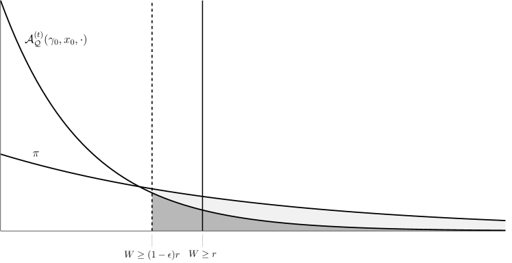
Figure 1: The diagram illustrates intuition for a discrepancy between the set $\{W\geq r\}$ for the adaptive process and the target measure and also $\{W\geq(1-\epsilon)r\}$ for small $\epsilon$.

Let $\partial A=\text{cl}(A)\setminus\text{int}(A)$ denote the boundary of a set $A$ where cl is the closure and int is the interior. Since $\mathbb{R}^{d}$ is convex, we have that $d(x,T)=d(x,\partial T)$ (see Lemma 20). Since $K=\{x\in\mathbb{R}^{d}:W(x)\leq r\}$ is compact, then $W$ is uniformly continuous on $K$. For $\epsilon\in(0,1)$, we can then choose $\delta_{\epsilon}$ depending on $\epsilon$ sufficiently small so that $W(x)\geq(1-\epsilon)r$ if $\text{dist}(x,T)\leq\delta_{\epsilon}$ and so

$$\mathbb{P}(X_{t}\in T^{\delta_{\epsilon}}) \leq\mathbb{P}(W(X_{t})\geq(1-\epsilon)r).$$

Markov’s inequality and (3) imply that

$$\mathbb{P}(W(X_{t})\geq(1-\epsilon)r)\leq\frac{\mathbb{E}\left[W^{\alpha}(X_{t})\right]}{(1-\epsilon)^{\alpha}r^{\alpha}}\leq\frac{H_{W(x_{0})^{\alpha},\varphi}^{-1}(t)}{(1-\epsilon)^{\alpha}r^{\alpha}}.$$

Optimizing, we get for $t$ large enough so that

$$r=\left(\frac{\alpha}{\kappa C(1-\epsilon)^{\alpha}}H_{W(x_{0})^{\alpha},\varphi}^{-1}(t)\right)^{\frac{1}{\alpha-\kappa}}\geq 1$$

and this yields the lower bound

$$\delta_{\epsilon}^{-1}\mathcal{W}_{\left\lVert\cdot\right\rVert\wedge 1}\left(\mathcal{A}_{\mathcal{Q}}^{(t)}(\gamma_{0},x_{0},\cdot),\pi\right) \geq\inf_{\xi\in\mathcal{C}\left[\mathcal{A}_{\mathcal{Q}}^{(t)}(\gamma_{0},x_{0},\cdot),\pi\right]}\xi(\{x,y:\left\lVert x-y\right\rVert>\delta_{\epsilon}\})$$

$$\geq\frac{C}{r^{\kappa}}-\frac{H_{W(x_{0})^{\alpha},\varphi}^{-1}(t)}{(1-\epsilon)^{\alpha}r^{\alpha}}.$$

$$\geq(1-\epsilon)^{\frac{\alpha\kappa}{\alpha-\kappa}}\frac{M}{H_{W(x_{0})^{\alpha},\varphi}^{-1}(t)^{\frac{\kappa}{\alpha-\kappa}}}$$

where $M$ is defined by (4). The conclusion follows since $\epsilon$ is arbitrary. ∎

An interpretation of Theorem 4 is the best possible rate of convergence for adaptive MCMC satisfying (3) for target measure satisfying (2). The conclusion of Theorem 4 can also be extended to general path-connected state spaces $\mathcal{X}$. The mild assumption of compact level sets for the function $W$ often holds in many applications. However, there is a significant drawback to the Wasserstein lower bound being the constant is non-explicit compared to the explicit lower bound in total variation.

What is surprising about the lower bounds in this section is the requirement only on the Markov family $(\mathcal{P}_{\gamma})_{\gamma\in\mathcal{Y}}$ to satisfy (3) and does not directly depend on an adaptation strategy. For example, it is common scenario in adaptive MCMC for the parameters space $\mathcal{Y}$ to be compact. In this case, the simultaneous growth condition (3) often holds if a Markov kernel satisfies some mild regularity conditions and (3) holds with only fixed parameters.

Example 5.

(Adaptive Unadjusted Langevin algorithm) Consider the multivariate Student’s t-distribution $\pi$ on $\mathbb{R}^{d}$ with $d\geq 1$ and $v>0$ degrees of freedom. The Lebesgue density is defined by

$$D_{\pi}(x)=\frac{(v+d)/2}{\Gamma(v/2)(v\pi)^{d/2}}\exp(-U(x))$$

where $U(x)=\frac{v+d}{2}\log(1+\left\lVert x\right\rVert^{2})$. The adapted unadjusted Langevin process $(\Gamma_{t},X_{t})_{t\geq 0}$ on $(0,1)\times\mathbb{R}^{d}$ defined by

$$X_{t+1}=X_{t}-\Gamma_{t+1}\nabla U(x)+\sqrt{2\Gamma_{t+1}}Z_{t+1}$$

where $\Gamma_{t+1}\in(0,1)$ and $Z_{t+1}$ is an independent standard normal random vector. Subgeometric drift conditions have been shown for unadjusted Langevin in the non-adaptive case for heavy tailed target measures [Kamatani, 2009].

Let $\alpha>0$ and $W(x)=(1+\left\lVert x\right\rVert^{2})^{(v+d)/2}$. By Ito’s formula, for large enough $\left\lVert x\right\rVert$, there is a constant $\epsilon>0$ such that the second term is bounded using the moment generating function of non-central chi-square random variables by

$$\mathbb{E}\left[W^{\alpha}(X_{t+1})|\Gamma_{t+1}=\gamma,X_{t}=x\right]-W^{\alpha}(x)$$

$$=\mathbb{E}\left[\int_{0}^{\gamma}\nabla W(x)^{\alpha}\cdot dX_{t}\right]+\mathbb{E}\left[\int_{0}^{\gamma}\text{tr}\left(\nabla^{2}W(x)^{\alpha}x\right)dt\right]$$

$$\leq\alpha(v+d)\left[-\gamma_{*}(v+2)+\alpha(v+d)+\epsilon\right]\left(1+\left\lVert x\right\rVert^{2}\right)^{\alpha(v+d)/2-1}.$$

It follows that for some constant $C_{\alpha}>0$ and for all $x,\gamma$,

$$\mathbb{E}\left[W^{\alpha}(X_{t+1})|\Gamma_{t+1}=\gamma,X_{t}=x\right]-W^{\alpha}(x)\leq C_{\alpha}W^{\alpha}(x)^{1-\frac{2}{\alpha(v+d)}}.$$

One has the lower bound for some constant $C>0$

$$\pi(W\geq r)\geq\frac{C}{r^{1-2/(v+d)}}.$$

If $v+d-2>0$, then by Theorem 4, then there is a constants $M>0$ such that

$$\inf_{\mathcal{Q}\in\mathcal{S}(\mathcal{X},\mathcal{Y})}\mathcal{W}_{\left\lVert\cdot\right\rVert\wedge 1}(\mathcal{A}_{\mathcal{Q}}^{(t)}(\gamma_{0},0,\cdot),\pi)\geq\frac{M}{(1+t)^{v+d-2}}.$$

Of particular interest is that the rate cannot be geometric even when considering weak convergence.

In certain situations, the tail probability decay on $\pi$ in (2) may be difficult to establish. In this case, we consider finding a function that is not integrable with respect to $\pi$, but this results in a trade-off of only a having a lower bound for a subsequence. An analogous result will also hold in total variation.

Theorem 6.

Let $\mathcal{X}=\mathbb{R}^{d}$ for $d\in\mathbb{Z}_{+}$. Assume for some Borel function $W:\mathcal{X}\to[1,\infty)$ such that $\int_{\mathcal{X}}Wd\pi=\infty$ but also for some $\alpha>1$ and some concave function $\varphi:(0,\infty)\to(0,\infty)$,

$$(\mathcal{P}_{\gamma}W^{\alpha})(x)-W(x)^{\alpha}\leq\varphi(W(x)^{\alpha})$$ (6)

holds for all $x,\gamma\in\mathcal{X}\times\mathcal{Y}$. Assume additionally for each $r>0$, the set $\{x\in\mathbb{R}^{d}:W(x)\leq r\}$ is compact. Then there is a constant $M_{*}>0$ and a subsequence $t_{n}\in\mathbb{Z}_{+}$ increasing to infinity such that for any $\epsilon\in(0,1)$ with $\alpha>1+\epsilon$,

$$\inf_{\mathcal{Q}\in\mathcal{S}(\mathcal{X},\mathcal{Y})}\mathcal{W}_{\left\lVert\cdot\right\rVert\wedge 1}\left(\mathcal{A}_{\mathcal{Q}}^{(t_{n},\mathcal{Q})}(\gamma_{0},x_{0},\cdot),\pi\right)\geq\frac{M_{*}}{\left(H_{W^{\alpha}(x_{0}),\varphi}^{-1}(t_{n})\right)^{\frac{1+\epsilon}{\alpha-1-\epsilon}}}.$$

Proof.

Since $\int_{\mathcal{X}}Wd\pi=\infty$, there is a sequence $(r_{n})_{n}$ with $\lim_{n}r_{n}=\infty$ such that with $T_{n}=\{x:W(x)\geq r_{n}\}$,

$$\pi(T_{n})\geq\frac{2^{\alpha+1}}{r_{n}^{1+\epsilon}}.$$

The conclusion follows by Theorem 4. ∎

3 Subgeometric upper bounds for adaptive MCMC

This section is dedicated to studying conditions such that an upper bound convergence rate can be obtained for adaptive MCMC comparable to the lower bounds in the previous section. We first consider an alternative to the diminishing adaptation condition [Roberts and Rosenthal, 2007] that is stronger in the sense that it requires a specified rate of decay.

Definition 7.

An adaptive process satisfies expected diminishing adaptation with function $G:\mathbb{Z}_{+}\to(0,\infty)$ strictly decreasing to infinity if and for all $t\in\mathbb{Z}_{+}$,

$$\sup_{x\in\mathcal{X}}\mathbb{E}\left[\left\lVert\mathcal{P}_{\Gamma_{t+1}}(x,\cdot)-\mathcal{P}_{\Gamma_{t}}(x,\cdot)\right\rVert_{\text{TV}}\mid X_{t}=x\right]\leq G(t).$$ (7)

Proposition 17 ensures Borel measurability of the total variation in (7). One way to satisfy this condition is if $\rho$ is a metric on $\mathcal{Y}$ and $\sup_{x}\mathbb{E}\left[\rho(\Gamma_{t+1},\Gamma_{t})\mid X_{t}=x\right]\leq G(t)$, then the expected diminishing adaptation condition can be shown through Lipschitz continuity of $\mathcal{P}_{\gamma}$. For example, if for each $x\in\mathcal{X}$, $\gamma\mapsto\mathcal{P}_{\gamma}(x,\cdot)$ is $\rho$-Lipschitz with constant $L_{x}$, then

$$\sup_{x\in\mathcal{X}}\left\lVert\mathcal{P}_{\Gamma_{t+1}}(x,\cdot)-\mathcal{P}_{\Gamma_{t}}(x,\cdot)\right\rVert_{\text{TV}}\leq\left(\sup_{x\in\mathcal{X}}L_{x}\right)\rho(\Gamma_{t+1},\Gamma_{t}).$$

This has been shown to hold generally for adaptive Metropolis-Hastings with symmetric proposals [Andrieu and Moulines, 2006]. Next, we consider a simultaneous version of a subgeometric drift condition on the Markov family.

Definition 8.

A Markov family $(\mathcal{P}_{\gamma})_{\gamma\in\mathcal{Y}}$ satisfies a simultaneous subgeometric drift condition if there is a Borel function $V:\mathcal{X}\to[1,\infty)$ and a concave function $\varphi:[0,\infty)\to[0,\infty)$ strictly increasing to infinity with $\lim_{v\to\infty}\varphi(v)/v=0$ and a constant $K\geq 0$ such that

$$(\mathcal{P}_{\gamma}V)(x)-V(x)\leq-\varphi(V(x))+K$$ (8)

holds for every $x,\gamma\in\mathcal{X}\times\mathcal{Y}$.

Here we assume $\lim_{v\to\infty}\varphi(v)/v=0$ to exclude the geometric case. Subgeometric drift conditions for Markov chains has been studied previously [Jarner and Roberts, 2002, Douc et al., 2004] but we adjust the previous conditions to hold over feasible tuning parameters $\mathcal{Y}$. We now combine this drift condition with a simultaneous local contracting condition.

Definition 9.

A Markov family $(\mathcal{P}_{\gamma})_{\gamma\in\mathcal{Y}}$ satisfies a simultaneously locally contracting condition on a set $C\subseteq\mathcal{X}\times\mathcal{X}$ if there is a constant $\alpha\in(0,1)$ where

$$\left\lVert\mathcal{P}_{\gamma}(x,\cdot)-\mathcal{P}_{\gamma}(y,\cdot)\right\rVert_{\text{TV}}\leq 1-\alpha$$ (9)

holds for all $x,y\in C$ and $\gamma\in\mathcal{Y}$.

Local coupling conditions have been studied in the subgeometric case for Markov chains [Durmus et al., 2016]. For example, a minorization condition can be used to verify the Markov family is simultaneously locally contracting (see [Roberts and Rosenthal, 2007]). Under these three conditions, we can establish an upper bound for the adaptation process.

Theorem 10.

Assume the expected diminishing adaptation condition (7) holds with $G(\cdot)$ decreasing to infinity. Additionally assume the following assumptions hold for the Markov family $(\mathcal{P}_{\gamma})_{\gamma\in\mathcal{Y}}$:

1. $\pi\mathcal{P}_{\gamma}=\pi$ for all $\gamma\in\mathcal{Y}$.

2. A simultaneously subgeometric drift condition (8) holds with a Borel function $V:\mathcal{X}\to[0,\infty)$.

3. A simultaneous locally contracting condition (9) holds on the set $C=\{x,y\in\mathcal{X}\times\mathcal{X}:V(x)+V(y)\leq 2K/(1-\delta)\}$ for some $\delta\in(0,1)$.

Then for all $\epsilon\in(0,1)$ and all $t\in\mathbb{Z}_{+}$,

$$\left\lVert\mathcal{A}_{\mathcal{Q}}^{(T_{\epsilon,t}+t)}((\gamma_{0},x_{0}),\cdot)-\pi\right\rVert_{\text{TV}}\leq\frac{\delta+\left[r(1)+1\right][V(x_{0})+\int Vd\pi+KT_{\epsilon,t}+C}{\delta H_{1,\varphi}^{-1}\left(\frac{t}{-\log(H_{1,\varphi}^{-1}(t))/\log(1-\alpha)+1}\right)}+\epsilon$$

where $T_{\epsilon,t}=(1/G)^{-1}(t^{2}/\epsilon)$ and

$$r(\cdot)=\varphi(H_{1,\varphi}^{-1}(\cdot)),\hskip 10.00002ptR=\varphi^{-1}(2K/(1-\delta)), C=\left[r(1)+1\right]\left\{R+\frac{r(1)}{r(0)}(R+4K)\right\}.$$

Theorem 10 requires satisfying expected diminishing adaptation (7) with a sufficiently fast rate. Table 1 compares approximate upper bounds for different combinations of $\varphi(\cdot)$ and $G(\cdot)$. The upper and lower bounds may be also combined and in particular, Theoerem 10 can guarantee the adaptive process approximately achieves the lower bound rate if the adaptation diminishes sufficiently fast. For example, if in addition to the assumptions of Theorem 10, there are constants $C,\kappa>0$ such that

$$\pi(V\geq r)\geq Cr^{-\kappa}, (\mathcal{P}_{\gamma}V^{2\kappa})(x)-V(x)^{2\kappa}\leq\varphi(V(x)^{2\kappa})$$

holds for every $x,\gamma\in\mathcal{X}\times\mathcal{Y}$. Then Theorem 1 and Theorem 10 imply some constants $M^{*},\alpha>0$ such that

$$\frac{C^{2}}{4H_{V(x_{0})^{2\kappa},\varphi}^{-1}(t)}\leq\left\lVert\mathcal{A}_{\mathcal{Q}}^{t}((\gamma_{0},x_{0}),\cdot)-\pi\right\rVert_{\text{TV}}\leq\frac{M^{*}T_{\epsilon,t}}{H_{1,\varphi}^{-1}\left(\frac{t}{-\log(H_{1,\varphi}^{-1}(t))/\log(1-\alpha)+1}\right)}+\epsilon$$

holds for all $t$ and $\epsilon$. Similarly, Theorem 4 can be used to give a weak lower bound. As an example, consider a target measure on $\mathbb{R}^{d}$ with potential $U:\mathbb{R}^{d}\to\mathbb{R}$ defined by $\pi(dx)\propto\exp(-U(x))dx$ and Lyapunov function defined by $\exp(\kappa U(x))$ for $\alpha>0$. Then with $\alpha<1$, this can be used to obtain an upper bound and with $\alpha>1$, this can be used to obtain a lower bound.

Examples of upper bound rates from Theorem 10
G(t)	$\varphi(w)=cw^{\beta},\beta\in(0,1)$	$\varphi(x)=c(x+K)/\log(x+K)^{\beta},\beta\in(0,1)$
$\exp(-\alpha t),\alpha>0$	$\propto\frac{\log(t)}{(1+(1-\beta)ct)^{1/(1-\beta)}}$	$\propto\log(t)\exp\left(-(1+\beta)ct^{\frac{1}{1+\beta}}\right)$
$\exp(-t^{\alpha}),\alpha\in(0,1)$	$\propto\frac{\log(t)^{1/\alpha}}{(1+(1-\beta)ct)^{1/(1-\beta)}}$	$\propto\log(t)^{1/\alpha}\exp\left(-(1+\beta)ct^{\frac{1}{1+\beta}}\right)$
$t^{-\alpha},\alpha>1$	$\propto\frac{t^{2/\alpha}}{(1+(1-\beta)ct)^{1/(1-\beta)}}$	$\propto t^{2/\alpha}\exp\left(-(1+\beta)ct^{\frac{1}{1+\beta}}\right)$

Table 1: Upper bound convergence rate comparisons from Theorem 10 for different combinations of $\varphi(\cdot)$ and $G(\cdot)$. The table entries specify a convergence rate upper bound up to an explicit constant.

Proof of Theorem 10.

We first specify a finite adaptation plan $\mathcal{Q}^{T}$ with a time $T\in\mathbb{Z}_{+}$ defining a stopping point of adaptation. This defines an adaptive process where for all $t\geq T$, $\Gamma_{t}=\Gamma_{T}$ and $(\Gamma_{t},X_{t})|(\Gamma_{s},X_{s})_{s\leq t-1}\sim\delta_{\Gamma_{T}}(\cdot)\mathcal{P}_{\Gamma_{T}}(X_{t-1},\cdot)$ where $\delta_{\Gamma_{T}}$ is the Dirac measure at $\Gamma_{T}$. Using the finite adaptation process, we have the upper bound via the triangle inequality

$$\left\lVert\mathcal{A}_{\mathcal{Q}}^{(T+t)}((\gamma_{0},x_{0}),\cdot)-\pi\right\rVert_{\text{TV}}$$

$$\leq\left\lVert\mathcal{A}_{\mathcal{Q}}^{(T+t)}((\gamma_{0},x_{0}),\cdot)-\mathcal{A}_{\mathcal{Q}^{T}}^{(T+t)}((\gamma_{0},x_{0}),\cdot)\right\rVert_{\text{TV}}+\left\lVert\mathcal{A}_{\mathcal{Q}^{T}}^{(T+t)}((\gamma_{0},x_{0}),\cdot)-\pi\right\rVert_{\text{TV}}.$$ (10)

We will bound each term on the right hand side of (10) separately. For the first term in (10), fix $\epsilon\in(0,1)$ and choose $T_{\epsilon,t}=(1/G)^{-1}(t^{2}/\epsilon)$. Using the triangle inequality, we have that

$$\sup_{x\in\mathcal{X}}\mathbb{E}\left[\left\lVert\mathcal{P}_{\Gamma_{T+t}}(x,\cdot)-\mathcal{P}_{\Gamma_{T}}(x,\cdot)\right\rVert_{\text{TV}}\mid X_{T+t-1}=x\right]$$

$$\leq\sum_{s=1}^{t}\sup_{x\in\mathcal{X}}\mathbb{E}\left[\left\lVert\mathcal{P}_{\Gamma_{T+s}}(x,\cdot)-\mathcal{P}_{\Gamma_{T+s-1}}(x,\cdot)\right\rVert_{\text{TV}}\mid X_{T+s-1}=x\right]$$

$$\leq tG(T)$$

$$\leq\epsilon/t.$$

Since $\mathcal{X}$ is Polish, Proposition 17 ensures the total variation is Borel measurable.

Let $(\Gamma_{t},X_{t})_{t\geq 0}$ be an adaptive process initialized at $x_{0},\gamma_{0}$ and $(\Gamma^{\prime}_{t},X^{\prime}_{t})_{t\geq 0}$ be the finite adaptation process initialized similarly. Since both of these processes are initialized at the same point, we can construct a coupling where $X_{s}=X_{s}^{\prime}$ for $s\leq T$ and

$$\mathbb{P}\left(X_{t+T}=Y_{t+T}\right) =\mathbb{P}\left(X_{t+T}=Y_{t+T}|X_{t+T-1}=Y_{t+T-1}\right)\mathbb{P}\left(X_{t+T-1}=Y_{t+T-1}\right)$$

$$\geq(1-\epsilon/t)\mathbb{P}\left(X_{t+T-1}=Y_{t+T-1}\right)$$

$$\geq(1-\epsilon/t)^{t}$$

$$\geq 1-\epsilon.$$

Since $\mathcal{X}$ is Polish, then it follows immediately that the optimal coupling is controlled by this coupling we have constructed so that

$$\left\lVert\mathcal{A}_{\mathcal{Q}}^{(T_{\epsilon,t}+t)}((\gamma_{0},x_{0}),\cdot)-\mathcal{A}_{\mathcal{Q}^{T_{\epsilon,t}}}^{(T_{\epsilon,t}+t)}((\gamma_{0},x_{0}),\cdot)\right\rVert_{\text{TV}}\leq\mathbb{P}\left(X_{t+T}\not=Y_{t+T}\right)\leq\epsilon.$$

To bound the second term in (10), the following is adapted from previous arguments for subgeometric upper bounds for non-adapted Markov chains [Durmus et al., 2016], but modified for adaptive MCMC, and the constants are improved and explicit. Since $\mathcal{X}$ is Polish, there is a Borel measurable conditional total variation distance by [Villani, 2009, Theorem 4.8] so that

$$\left\lVert\mathcal{A}_{\mathcal{Q}^{T}}^{(T+t)}((\gamma_{0},x_{0}),\cdot)-\pi\right\rVert_{\text{TV}} \leq\mathbb{E}\left[\left\lVert\mathcal{P}_{\Gamma_{T}}^{t}(X_{T},\cdot)-\pi\right\rVert_{\text{TV}}\right].$$

Let $\tau_{C}=\inf\{n\geq 1:X_{n},Y_{n}\in C\}$ be the first hit time to the set $C$. For $n\in\mathbb{Z}_{+}$, let $\theta_{n}$ denote the shift operator applied $n$ times so that $\theta_{n}(X_{i})=X_{i+n}$ for all $i\in\mathbb{Z}_{+}$. Define the successive hit times to $C$ recursively by

$$\tau_{1}=\tau_{C}, \tau_{n+1}=\tau_{n}+\tau_{C}\circ\theta_{\tau_{n}}=\sum_{k=1}^{n+1}\tau_{k}$$

for each $n\in\mathbb{Z}_{+}$. The inverse function theorem implies the derivative $r(s)=\frac{d}{ds}H^{-1}_{1,\varphi}(s)=\varphi(H^{-1}_{1,\varphi}(s))$ for $s\geq 0$. Thus, $H_{1,\varphi}^{-1}$ is convex since its derivative is monotone increasing by Lemma 18. By Markov’s inequality and Jensen’s inequality,

$$\mathbb{P}(\tau_{m}\geq t) \leq\frac{\mathbb{E}\left[H_{1,\varphi}^{-1}\left(\frac{1}{m}\sum_{k=1}^{m}\tau_{k}\right)\right]}{H_{1,\varphi}^{-1}(t/m)}$$

$$\leq\frac{\frac{1}{m}\sum_{k=1}^{m}\mathbb{E}\left[H_{1,\varphi}^{-1}(\tau_{k})\right]}{H_{1,\varphi}^{-1}(t/m)}.$$

For any $t,m\in\mathbb{Z}_{+}$ with $t\geq m$, the local coupling condition (9) implies an upper bound via a coupling argument with [Jarner and Tweedie, 2001, Lemma 3.1] so that for all $\gamma\in\mathcal{Y}$ and $x,y\in\mathcal{X}$,

$$\left\lVert\mathcal{P}_{\gamma}^{t}(x,\cdot)-\mathcal{P}_{\gamma}^{t}(y,\cdot)\right\rVert_{\text{TV}} \leq\inf_{\xi\in\mathcal{C}\left(\mathcal{P}_{\gamma}^{t}(x,\cdot),\mathcal{P}_{\gamma}^{t}(y,\cdot)\right)}\xi(\{u,v:u\not=v,\tau_{m}<t\})+\mathbb{P}(\tau_{m}\geq t)$$

$$\leq(1-\alpha)^{m}+\mathbb{P}\left(\sum_{k=1}^{m}\tau_{k}>t\right)$$

$$\leq(1-\alpha)^{m}+\frac{\frac{1}{m}\sum_{k=1}^{m}\mathbb{E}\left[H_{1,\varphi}^{-1}(\tau_{k})\right]}{H_{1,\varphi}^{-1}(t/m)}.$$

Since $\varphi$ is concave, it is subadditive so $\varphi(V(x)+V(y))\leq\varphi(V(x))+\varphi(V(y))$. Since $\varphi$ is strictly increasing, by the drift condition,

$$(\mathcal{P}_{\gamma}V)(x)+(\mathcal{P}_{\gamma}V)(y)-[V(x)+V(y)] \leq-[\varphi(V(x))+\varphi(V(y))]+2K$$

$$\leq-[\varphi(V(x)+V(y))]+2K$$

holds for all $x,y\in\mathcal{X}$. Using Lemma 19,

$$(\mathcal{P}_{\gamma}V)(x)+(\mathcal{P}_{\gamma}V)(y)-[V(x)+V(y)]\leq-\delta[\varphi(V(x)+V(y))]+(R+2K)I_{C}(x,y).$$

By [Douc et al., 2004, Proposition 2.2],

$$\sup_{x,y\in C}\mathbb{E}_{x,y}\left(\sum_{i=0}^{\tau_{C}-1}r(i)\right)\leq\frac{\varphi^{-1}(2K/(1-\delta))}{\delta}+\frac{(R+2K)r(1)}{\delta r(0)}.$$

We have that $r(\cdot)=\varphi(H_{1,\varphi}^{-1}(\cdot))$ is log-concave and so $r(s+t)\leq r(s)r(t)$ for all $t,s\geq 0$ [Douc et al., 2004, see the proof of Proposition 2.1]. We then have the upper bound for $k\geq 2$,

$$\mathbb{E}\left[H_{1,\varphi}^{-1}(\tau_{k})\right] =\mathbb{E}\left[\mathbb{E}_{X_{\tau_{k-1}}}\left(\int^{\tau_{k}}_{0}r(s)ds\right)\right]$$

$$\leq\mathbb{E}\left[\mathbb{E}_{X_{\tau_{k-1}}}\left(\sum_{i=1}^{\tau_{C}}r(i)\right)\right]$$

$$\leq\mathbb{E}\left[\mathbb{E}_{X_{\tau_{k-1}}}\left(r(\tau_{C})\right)\right]-r(0)+\mathbb{E}\left[\mathbb{E}_{X_{\tau_{k-1}}}\left(\sum_{i=0}^{\tau_{C}-1}r(i)\right)\right]$$

$$\leq r(1)\mathbb{E}\left[\mathbb{E}_{X_{\tau_{k-1}}}\left(r(\tau_{C}-1)\right)\right]-r(0)+\mathbb{E}\left[\mathbb{E}_{X_{\tau_{k-1}}}\left(\sum_{i=0}^{\tau_{C}-1}r(i)\right)\right]$$

$$\leq[r(1)+1]\mathbb{E}\left[\mathbb{E}_{X_{\tau_{k-1}}}\left(\sum_{i=0}^{\tau_{C}-1}r(i)\right)\right]-r(0)$$

$$\leq\frac{r(1)+1}{\delta}\left\{R\left(1+\frac{r(1)}{r(0)}\right)+\frac{2Kr(1)}{r(0)}\right\}.$$

For $k=1$, similarly, we have

$$\mathbb{E}\left[H_{1,\varphi}^{-1}(\tau_{C})\right]\leq\frac{r(1)+1}{\delta}\left\{V(x)+V(y)+\frac{Rr(1)}{r(0)}+\frac{2Kr(1)}{r(0)}\right\}.$$

Combining these upper bounds,

$$\mathbb{E}\left[H_{1,\varphi}^{-1}\left(\frac{1}{m}\sum_{k=1}^{m}\tau_{k}\right)\right]\leq\frac{r(1)+1}{\delta}\left\{V(x)+V(y)+R+\frac{r(1)}{r(0)}(R+4K)\right\}.$$

The simultaneous subgeometric drift condition (8) implies

$$\mathbb{E}\left[V(X_{T})\right]\leq V(x_{0})+KT.$$

Choosing $m\equiv m_{t}=\lceil\log(H_{1,\varphi}^{-1}(t))/\log(1/(1-\alpha))\rceil$, we have the upper bound

$$\left\lVert\mathcal{A}_{\mathcal{Q}^{T}}^{(T+t)}((\gamma_{0},x_{0}),\cdot)-\pi\right\rVert_{\text{TV}}$$

$$\leq(1-\alpha)^{m_{t}}+\frac{\left[r(1)+1\right]\left\{V(x_{0})+KT+\int Vd\pi+R+\frac{r(1)}{r(0)}(R+4K)\right\}}{\delta H_{1,\varphi}^{-1}(t/m_{t})}$$

$$\leq\frac{\delta+\left[r(1)+1\right]\left\{V(x_{0})+KT+\int Vd\pi\right\}+C}{\delta H_{1,\varphi}^{-1}(t/m_{t})}.$$

∎

4 Example: adaptive Metropolis-Hastings independence sampler

In many cases, it is difficult to choose a proposal for Metropolis-Hastings that approximately matches the tail behavior of a complex target measure and adaptive MCMC is often employed. The point of this toy example is to concretely demonstrate this scenario. We will use the upper and lower bounds on the convergence to investigate and the sensitivity to different adaptation strategies. Consider the target measure $\pi(dx)=\exp(-x)I_{[0,\infty)}(x)dx$. Let $(\gamma_{*},\gamma^{*})$ be the interval for some potential tuning parameters $1<\gamma_{*}<\gamma^{*}$ and consider a Metropolis-Hastings Markov chain with independent proposal $\gamma\exp(-\gamma x)I_{[0,\infty)}(x)$ and Markov kernel defined for $x,\gamma\in[0,\infty)\times(\gamma_{*},\gamma^{*})$ and all Borel sets $A\subseteq[0,\infty)$ by

$$\mathcal{P}_{\gamma}(x,A)=\int_{A}a_{\gamma}(x,y)\gamma\exp(-\gamma y)dy+\delta_{x}(A)R_{\gamma}(x)$$ (11)

where the acceptance function is $a_{\gamma}(x,y)=\exp\left[(\gamma-1)(y-x)\right]\wedge 1$ and the rejection probability is $R_{\gamma}(x)=1-\int_{0}^{\infty}a_{\gamma}(x,y)\gamma\exp(-\gamma y)dy$. Since we restrict $\gamma>1$, the tail probabilities of the proposal and the Metropolis-Hastings kernel are lighter than the target. Due to this restriction, we will have a polynomial lower bound over any possible adaptation plan.

Proposition 11.

Let $\mathcal{A}_{\mathcal{Q}}^{(t)}(\gamma_{0},x_{0},\cdot)$ be the marginal of the adaptive independent Metropolis-Hastings process at time $t\in\mathbb{Z}_{+}$ from (11) with adaptation parameter set $(\gamma_{*},\gamma^{*})$ and initialized at $x_{0},\gamma_{0}\in(0,\infty)\times(\gamma_{*},\gamma^{*})$. Then

$$\inf_{\mathcal{Q}\in\mathcal{S}([0,\infty),(\gamma_{*},\gamma^{*}))}\left\lVert\mathcal{A}_{\mathcal{Q}}^{(t)}(\gamma_{0},0,\cdot)-\pi\right\rVert_{\text{TV}}\geq\frac{M_{*}}{\left(c_{*}t+1\right)^{\frac{1}{\gamma_{*}-1}}}$$

where $M_{*}=\gamma_{*}^{-1/(\gamma_{*}-1)}-\gamma_{*}^{-\gamma_{*}/(\gamma_{*}-1)}$ and $c_{*}=\frac{\gamma^{*}}{\gamma_{*}-1}+\gamma^{*}-1$.

Proof.

Define $W(x)=\exp(x)$, and we have by a standard computation $\pi(W(x)\geq r)=r^{-1}$. Assume $1<\gamma_{*}<\gamma$. For $\alpha<\gamma$, the identity holds

$$(\mathcal{P}_{\gamma}W^{\alpha})(x)-W^{\alpha}(x)$$

$$=\int_{[0,\infty)}\exp(\alpha y)1\wedge\left\{\exp\left[(\gamma-1)(y-x)\right]\right\}\gamma\exp(-\gamma y)dy-\exp(\alpha x)\mathbb{E}\left(a_{\gamma}(x,Y)\right).$$

We also have for any $\alpha<\gamma$,

$$\int_{[0,\infty)}\exp(\alpha y)1\wedge\left\{\exp\left[(\gamma-1)(y-x)\right]\right\}\gamma\exp(-\gamma y)dy$$

$$=\frac{\gamma\exp\left[(1-\gamma)x\right]}{\alpha-1}\int_{0}^{x}(\alpha-1)\exp\left[(\alpha-1)y\right]dy$$

$$\hskip 15.00002pt+\frac{\gamma}{\gamma-\alpha}\int_{x}^{\infty}(\gamma-\alpha)\exp\left[-(\gamma-\alpha)y\right]dy$$

$$=\left\{\frac{\gamma}{\alpha-1}+\frac{\gamma}{\gamma-\alpha}\right\}\exp\left[-(\gamma-\alpha)x\right]-\frac{\gamma}{\alpha-1}\exp\left[-(\gamma-1)x\right].$$ (12)

Using (12), $\mathbb{E}\left(a_{\gamma}(x,Y)\right)=\gamma\exp((1-\gamma)x)+(1-\gamma)\exp(-\gamma x).$ So then

$$(\mathcal{P}_{\gamma}W^{\alpha})(x)-W^{\alpha}(x)$$

$$=\left\{\frac{\gamma}{\alpha-1}+\frac{\gamma}{\gamma-\alpha}+\gamma-1\right\}\exp\left[-(\gamma-\alpha)x\right]-\frac{\gamma}{\alpha-1}\exp\left[-(\gamma-1)x\right]-\gamma W(x)^{\frac{1+\alpha-\gamma}{\alpha}}.$$

It follows that

$$(\mathcal{P}_{\gamma}W^{\gamma_{*}})(x)-W^{\gamma_{*}}(x) =\left\{\frac{\gamma}{\gamma_{*}-1}+\frac{\gamma}{\gamma-\gamma_{*}}+\gamma-1\right\}\exp(-(\gamma-\gamma_{*})x)$$

$$\hskip 15.00002pt-\frac{\gamma}{\gamma_{*}-1}\exp(-(\gamma-1)x)-\gamma W^{\gamma_{*}}(x)^{\frac{1+\gamma_{*}-\gamma}{\gamma_{*}}}$$

$$\leq c_{*}.$$ (13)

With the upper bound in (13), we can now use Theorem 1 with $\varphi\equiv c^{*}$, $\kappa=1$, and $\alpha=\gamma_{*}$. We then have the lower bound

$$\left\lVert\mathcal{A}_{\mathcal{Q}}^{(t)}(\gamma_{0},x_{0},\cdot)-\pi\right\rVert_{\text{TV}}\geq\frac{M_{*}}{\left[c_{*}t+\exp(\gamma_{*}x_{0})\right]^{\frac{1}{\gamma_{*}-1}}}$$

holds for every $t\in\mathbb{Z}_{+}$ uniformly in the adaptation strategy $\mathcal{Q}$. ∎

In Table 2, we compute the lower bound in Proposition 11 for different choices of $(\gamma_{*},\gamma^{*})$. The large values from Table 2 illustrate that even in this toy example, it is possible to observe poor convergence behavior of adaptive MCMC with certain tuning parameter sets independently of the adaptation strategy. However, this limitation on the convergence rate can be avoided if the adaptation plan is capable of crossing the critical boundary $\gamma=1$. By Theorem 4, the lower bound rate in Proposition 11 will be the same even when converging weakly.

Lower bound computations from Proposition 11
Iteration	$(\gamma_{*},\gamma^{*})=(3,5)$	$(\gamma_{*},\gamma^{*})=(4,6)$	$(\gamma_{*},\gamma^{*})=(8,10)$
$10^{3}$	$0.0048$	$0.0247$	$0.173$
$10^{4}$	$0.0015$	$0.0115$	$0.125$
$10^{5}$	$0.0005$	$0.00532$	$0.0898$
$10^{6}$	$0.0001$	$0.00247$	$0.0646$

Table 2: Lower bound computations from Propositon 11 for the adaptive Metropolis-Hastings independence sampler.

We now look at upper bounds from Section 3 where we require adaptation is restricted to a compact set. This is a commonly used strategy in adaptive MCMC [Pompe et al., 2020].

Proposition 12.

For $t\in\mathbb{Z}_{+}$, let $\mathcal{A}_{\mathcal{Q}}^{(t)}(\gamma_{0},x_{0},\cdot)$ be the marginal of an adaptive independent Metropolis-Hastings process and $M_{*},c_{*}$ defined in Proposition 11. Assume for each $t\in\mathbb{Z}_{+}$, $\mathcal{P}_{\Gamma_{t+1}}(x,\cdot)=\mathcal{P}_{\Gamma_{t}}(x,\cdot)$ for all $x\geq r$ for some $r>0$ and

$$\sup_{x\in\mathcal{X}}\mathbb{E}\left[\left\lVert\Gamma_{t+1}-\Gamma_{t}\right\rVert_{F}\mid X_{t}=x\right]\leq G(t)$$

for some function $G(\cdot)$ strictly decreasing to infinity. Additionally, assume $\gamma^{*}<2-\epsilon$ for some $\epsilon\in(0,1)$. Then for all $\delta\in(0,1)$ and $t\in\mathbb{Z}_{+}$ with $T_{\delta,t}=(1/G)^{-1}\left(Jt^{2}/\delta\right)$,

$$\frac{M_{*}}{\left[c_{*}(T_{\delta,t}+t)+1\right]^{\frac{1}{\gamma_{*}-1}}}\leq \left\lVert\mathcal{A}_{\mathcal{Q}}^{(T_{\delta,t}+t)}((\gamma_{0},0),\cdot)-\pi\right\rVert_{\text{TV}} \leq\frac{2\left[r(1)+1\right]KT_{\delta,t}+C}{\left[1+c\frac{t}{-\log(1+ct)/\log(1-\alpha)+1}\right]^{\frac{1-\epsilon}{\gamma^{*}-1}}}+\delta$$

where

$$J=2/\gamma_{*}^{2}+r+\frac{1}{\gamma_{*}},c=\frac{\gamma^{*}-1}{1-\epsilon},K=\frac{\gamma^{*}}{\gamma_{*}-1+\epsilon},\alpha=\frac{\gamma_{*}}{(2K)^{\frac{\gamma*^{-}1}{1-\epsilon}}},r(1)=\left(c+1\right)^{\frac{2-\epsilon-\gamma^{*}}{\gamma^{*}-1}},$$

$$R=(4K)^{\frac{1-\epsilon}{2-\epsilon-\gamma^{*}}},C=1+2\left[r(1)+1\right][1+\epsilon^{-1}]+\left[r(1)+1\right]\left\{R+r(1)(R+4K)\right\}.$$

Proof.

We will use Theorem 10 to establish the upper bound. We first verify the expected diminishing adaptation condition (7). Let $\varphi:\mathbb{R}\to[0,1]$ and for $x>0$ and let $\psi_{x}(y)=\varphi(y)-\varphi(x)$. Then

$$\mathcal{P}_{\gamma^{\prime}}\varphi(x)-\mathcal{P}_{\gamma}\varphi(x)=\mathcal{P}_{\gamma^{\prime}}\psi_{x}(x)-\mathcal{P}_{\gamma}\psi_{x}(x)$$

$$=\int\psi_{x}(y)\left[a_{\gamma^{\prime}}(x,y)\gamma^{\prime}\exp(-\gamma^{\prime}y)-a_{\gamma}(x,y)\gamma\exp(-\gamma y)\right]dy$$

$$\leq|\gamma^{\prime}-\gamma|\int|y-x|\gamma^{\prime}\exp(-\gamma^{\prime}y)dy+\int|\gamma^{\prime}\exp(-\gamma^{\prime}y)-\gamma\exp(-\gamma y)|dy$$

$$\leq(2/\gamma_{*}^{2}+|x|)|\gamma^{\prime}-\gamma|+\frac{1}{\gamma_{*}}|\gamma^{\prime}-\gamma|.$$

Let $J=2/\gamma_{*}^{2}+r+\frac{1}{\gamma_{*}}$ and so expected diminishing adaptation (7) since

$$\sup_{x\in[0,\infty)}\mathbb{E}\left(\left\lVert\mathcal{P}_{\Gamma_{t+1}}(x,\cdot)-\mathcal{P}_{\Gamma_{t}}(x,\cdot)\right\rVert_{\text{TV}}\mid X_{t}=x\right) \leq J\sup_{|x|\leq r}\mathbb{E}\left(|\Gamma_{t+1}-\Gamma_{t}|\mid X_{t}=x\right)$$

$$\leq JG(t).$$

Next, we verify the simultaneous subgeometric drift condition. Let $V(x)=\exp(x)$, and using the identity (12), for $\epsilon\in(0,1)$,

$$(\mathcal{P}_{\gamma}V^{1-\epsilon})(x)-V^{1-\epsilon}(x)\leq\left\{\frac{\gamma^{*}}{\gamma_{*}-1+\epsilon}+\gamma^{*}-1\right\}-\gamma_{*}V(x)^{\frac{2-\epsilon-\gamma^{*}}{1-\epsilon}}.$$

Now we satisfy the simultaneous local coupling with a minorization condition. If $V(x)\leq R$, then $\exp((\gamma-1)x)\leq R^{\frac{\gamma-1}{1-\epsilon}}$. Define $\nu_{\gamma}(\cdot)=Z^{-1}\int_{\cdot}1\wedge\exp((\gamma-1)y)\gamma\exp(-\gamma y)dy$ where $Z$ is the normalizing constant. So then

$$\inf_{V(x)\leq R}\mathcal{P}_{\gamma}(x,\cdot)\geq\frac{\gamma_{*}}{R^{\frac{\gamma*^{-}1}{1-\epsilon}}}\nu_{\gamma}(\cdot).$$

∎

If adaptation diminishes fast enough, Proposition 12 shows the upper bound rate is essentially $(1+t)^{\frac{1-\epsilon}{1-\gamma^{*}}}$ and depends on the largest tuning parameter $\gamma^{*}$. This is due to the adaptation plan possibly concentrating on $\gamma^{*}$, which is farthest from the optimal choice. On the other hand, the lower bound rate $(1+t)^{\frac{1}{1-\gamma_{*}}}$ depends on the smallest tuning parameter $\gamma_{*}$ being closest to the optimal choice. In particular, there can be a gap in the upper and lower bounds on the convergence characterized by potential tuning parameters. In Table 3, we compare the upper bound convergence rates with $\epsilon=.01$, $G(t)=\exp(-t)$, and $\delta=(1+ct)^{\frac{1-\epsilon}{1-\gamma^{*}}}$. We observe that the upper bound is sensitive to the tuning of $\gamma^{*}$.

Upper bound computations from Proposition 12
Iteration $t$	$(\gamma_{*},\gamma^{*})=(1.2,1.5)$	$(\gamma_{*},\gamma^{*})=(1.2,1.6)$	$(\gamma_{*},\gamma^{*})=(1.2,1.7)$
$10^{3}$	$2.048\cdot 10^{-1}$	$7.859\cdot 10^{0}$	$7.368\cdot 10^{2}$
$10^{4}$	$2.217\cdot 10^{-3}$	$1.784\cdot 10^{-1}$	$2.867\cdot 10^{1}$
$10^{5}$	$2.379\cdot 10^{-5}$	$4.018\cdot 10^{-5}$	$1.106\cdot 10^{0}$
$10^{6}$	$2.550\cdot 10^{-7}$	$9.04\cdot 10^{-5}$	$4.26\cdot 10^{-2}$

Table 3: A comparison of the upper bounds from Proposition 12 for the adaptive Metropolis-Hastings independence sampler with $\epsilon=.01$, $G(t)=\exp(-t)$, and $\delta=(1+ct)^{\frac{1-\epsilon}{1-\gamma^{*}}}$.

5 Example: Adaptive random walk Metropolis

Adaptive random-walk Metropolis is a popular simulation algorithm for Bayesian statistics [Haario et al., 2001]. Let $U:\mathbb{R}^{d}\to\mathbb{R}$ and consider the target measure with with normalizing constant $Z=\int_{\mathbb{R}^{d}}\exp(-U(x))dx$ defined by $\pi(dx)=Z^{-1}\exp(-U(x))dx$. We make the following regularity assumptions on the target $\pi$ which have been used previously to show convergence results in MCMC [Douc et al., 2004]. Let $\left\lVert\cdot\right\rVert_{F}$ denote the Frobenius norm.

Assumption 13.

Suppose $U$ is continuous and twice continuously differentiable and there exists a minimum such that $x_{*}$ such that $U(x_{*})=0$. Assume there are constants $d_{k},D_{k},r>0$ for $k=1,2,3$ such that for all $x\in\mathbb{R}^{d}$ with $\left\lVert x\right\rVert\geq R$ for some $R>0$,

$$d_{1}\left\lVert x\right\rVert^{m}\leq U(x)\leq D_{1}\left\lVert x\right\rVert^{m},$$ (14)

$$d_{2}\left\lVert x\right\rVert^{m-1}\leq\left\lVert\nabla U(x)\right\rVert\leq D_{2}\left\lVert x\right\rVert^{m-1}, \frac{\nabla U(x)}{\left\lVert U(x)\right\rVert}\cdot\frac{x}{\left\lVert x\right\rVert}\geq r,$$ (15)

$$d_{3}\left\lVert x\right\rVert^{m-2}\leq\left\lVert\nabla^{2}U(x)\right\rVert_{F}\leq D_{3}\left\lVert x\right\rVert^{m-2}.$$ (16)

While Assumption (13) is strong, the Weibull distribution is one example (see [Fort and Moulines, 2000]). Let $g_{K}$ be a Lebesgue density on $\mathbb{R}^{d}$ used for the proposal supported on a compact set $K\subset\mathbb{R}^{d}$ satisfying

$$g_{K}(\xi)=g_{K}(\left\lVert\xi\right\rVert)\text{ for all }\xi\in\mathbb{R}^{d}, \inf_{\xi\in K}g_{K}(\xi)>0.$$ (17)

For $\gamma\in\mathcal{Y}$, define the random-walk Metropolis Markov family for $x\in\mathbb{R}^{d}$ and Borel $A\subseteq\mathbb{R}^{d}$ by

$$\mathcal{P}_{\gamma}(x,A)=\int_{A}a(x,x+\gamma^{1/2}\xi)g_{K}(\xi)d\xi+\delta_{x}(A)R_{\gamma}(x)$$ (18)

with acceptance function $a(x,y)=\exp[U(x)-U(y)]\wedge 1$, and rejection probability $R_{\gamma}(x)=1-\int_{\mathbb{R}^{d}}a(x,x+\gamma^{1/2}\xi)g_{K}(\xi)d\xi$. We define an adaptive random-walk Metropolis process by adapting the covariance of the proposal [Haario et al., 2001] with dynamics $\Gamma_{t}|(\Gamma_{s},X_{s})_{s\leq t-1}$ first updating the covariance matrix, and then $X_{t}|\Gamma_{t},X_{t-1}$ updating the current state with random-walk Metropolis.

For the tuning parameter set $\mathcal{Y}$, we consider the set of symmetric positive definite matrices on $\mathbb{R}^{d}$ such that the eigenvalues are bounded by constants $\lambda_{*},\lambda^{*}>0$, that is,

$$\mathcal{Y}=\left\{\gamma\in\mathbb{R}^{d\times d}:\lambda_{*}I\leq\gamma\leq\lambda^{*}I,\gamma^{T}=\gamma\right\}.$$ (19)

One example is to adapt a sample covariance matrix scaled by $h>0$ using the following identity

$$\Gamma_{t}=\frac{h}{t}\sum_{s=0}^{t}(X_{s}-\bar{X}_{t})(X_{s}-\bar{X}_{t})^{T}=\frac{t-1}{t}\Gamma_{t-1}+\frac{h}{t+1}(X_{t}-\bar{X}_{t-1})(X_{t}-\bar{X}_{t-1})^{T}$$ (20)

where $\bar{X}_{t}=(t+1)^{-1}\sum_{s=0}^{t}X_{s}$ [Haario et al., 2001, Andrieu and Moulines, 2006]. The set $\mathcal{Y}$ is convex and one way to ensure the updates remain in $\mathcal{Y}$ is to truncate the eigenvalues of (20).

Under Assumption (13), we first obtain a lower bound on the convergence rate for the adaptive random-walk Metropolis process.

Proposition 14.

For $t\in\mathbb{Z}_{+}$, let $\mathcal{A}_{\mathcal{Q}}^{(t)}(\gamma_{0},x_{0},\cdot)$ be the marginal of the adaptive random-walk Metropolis process initialized at $x_{0},\gamma_{0}\in\mathbb{R}^{d}\times\mathcal{Y}$ from the Metropolis-Hastings family (18) and adaptation parameter set (19). If Assumption (13) holds for $\pi$, then there are constants $c_{*}>0$ depending on $m$ and $M_{*}$ depending on $m$ and $x_{0}$ such that

$$\inf_{\mathcal{Q}\in\mathcal{S}(\mathcal{X},\mathcal{Y})}\mathcal{W}_{\left\lVert\cdot\right\rVert\wedge 1}\left(\mathcal{A}_{\mathcal{Q}}^{(t)}(\gamma_{0},x_{0},\cdot),\pi\right)\geq M_{*}\exp\left(-c_{*}{t}^{\frac{m}{2-m}}\right).$$

In order to proceed, we will first establish a simultaneous growth condition on the Markov family.

Lemma 15.

With $W(x)=\exp(U(x))$, there are constants $M_{0},N_{0},L>0$ depending on $m$ such that for any $\alpha>0$ and $x,\gamma\in\mathcal{X}\times\mathcal{Y}$,

$$(\mathcal{P}_{\gamma}W^{\alpha})(x)-W^{\alpha}(x) \leq M_{0}\alpha^{3-2/m}\left[\alpha-N_{0}\right]\varphi(W^{\alpha}(x))+L$$ (21)

where for $K_{m}=\exp(2/(m-2)+1)$ and $w\geq 1$,

$$\varphi(w)=\frac{w+K_{m}}{\log\left[w+K_{m}\right]^{2/m-2}}.$$

Proof.

Similar to [Fort and Moulines, 2000, Lemma B.4], using the fundamental theorem of calculus and (15)

$$\sup_{\xi\in K}\frac{W^{\alpha}(x+\gamma^{1/2}\xi)}{W^{\alpha}(x)} =1+\int_{0}^{1}\frac{W^{\alpha}(x+t\gamma^{1/2}\xi)}{W^{\alpha}(x)}\gamma\nabla U(x+t\gamma\xi)dt$$

$$\leq 1+\left\lVert\gamma\right\rVert\sup_{\xi\in K}\left\lVert\xi\right\rVert\sup_{\xi\in K}\frac{W^{\alpha}(x+t\gamma^{1/2}\xi)}{W^{\alpha}(x)}\int_{0}^{1}\left\lVert x+t\gamma^{1/2}\xi\right\rVert^{m-1}dt.$$

It follows that

$$\lim_{r\to\infty}\sup_{\left\lVert x\right\rVert\geq r}\sup_{\xi\in K}\frac{W^{\alpha}(x+\gamma^{1/2}\xi)}{W^{\alpha}(x)} \leq 1.$$

Using the fundamental theorem of calculus twice with (15) and (16), there is a constant $M>0$ such that for large enough $\left\lVert x\right\rVert$

$$\left|\frac{W^{\alpha}(x+\gamma^{1/2}\xi)}{W^{\alpha}(x)}-1-\alpha\gamma^{1/2}\nabla U(x)\cdot\xi\right|$$

$$\leq\int_{0}^{1}\frac{W^{\alpha}(x+tC\xi)}{W^{\alpha}(x)}\left\{\alpha^{2}[\gamma^{1/2}\nabla U(x+t\gamma^{1/2}\xi)\cdot\xi]^{2}+\alpha\xi\cdot\gamma^{1/2}\nabla^{2}U(x+t\gamma^{1/2}\xi)\gamma^{1/2}\xi\right\}(1-t)dt$$

$$\leq\alpha^{2}M\left\lVert x\right\rVert^{2(m-1)}.$$

Similarly, we obtain

$$\left|\exp(U(x)-U(x+\gamma^{1/2}\xi))-1+\gamma^{1/2}\nabla U(x)\cdot\xi\right|\leq M\left\lVert x\right\rVert^{2(m-1)}.$$

Let $r_{\gamma}(x)=\{y\in\mathbb{R}^{d}:U(x)<U(x+\gamma^{1/2}y)\}$ denote the rejection region. By [Fort and Moulines, 2000, Lemma B.3] combined with (15), there is a constant $a>0$ such that for large enough $\left\lVert x\right\rVert$

$$\int_{r_{\gamma}(x)}\left[\gamma^{1/2}\nabla U(x)\cdot\xi\right]^{2}g_{K}(\xi)d\xi\geq a\left\lVert\nabla U(x)\right\rVert^{2}.$$

Applying these bounds, for large enough $\left\lVert x\right\rVert$,

$$\frac{(\mathcal{P}_{\gamma}W^{\alpha})(x)}{W^{\alpha}(x)}-1$$

$$\leq\alpha\int_{\mathbb{R}^{d}}\gamma^{1/2}\nabla U(x)\cdot\xi a(x,x+\gamma^{1/2}\xi)g_{K}(\xi)d\xi+M\alpha^{2}\left\lVert x\right\rVert^{2(m-1)}$$

$$=\alpha\int_{r_{\gamma}(x)}\gamma^{1/2}\nabla U(x)\cdot\xi\left(\exp[U(x)-U(x+\gamma^{1/2}\xi)]-1\right)g_{K}(\xi)d\xi+M\alpha^{2}\left\lVert x\right\rVert^{2(m-1)}$$

$$\leq-\alpha\int_{r_{\gamma}(x)}\left[\gamma^{1/2}\nabla U(x)\cdot\xi\right]^{2}dG(\xi)+M\alpha^{2}\left\lVert x\right\rVert^{2(m-1)}$$

$$\leq-\alpha a\left\lVert\nabla U(x)\right\rVert^{2}+M\alpha^{2}\left\lVert x\right\rVert^{2(m-1)}.$$

Applying (14) and (15), there are constants $M_{0},N_{0},K_{m}>0$ such that $\left\lVert x\right\rVert$ sufficiently large

$$(\mathcal{P}_{\gamma}W^{\alpha})(x)-W^{\alpha}(x) \leq M_{0}\alpha\left[\alpha-N_{0}\right]\frac{W^{\alpha}(x)}{U(x)^{2/m-2}}$$

$$\leq M_{0}\alpha^{3-2/m}\left[\alpha-N_{0}\right]\frac{W^{\alpha}(x)+K_{m}}{\log(W^{\alpha}(x)+K_{m})^{2/m-2}}.$$

For small $\left\lVert x\right\rVert$, we have by continuity, the sub-level sets of $W$ are compact and $(\mathcal{P}_{\gamma}W^{\alpha})(x)-W^{\alpha}(x)$ is bounded on compact sets, so the conclusion follows at once. ∎

We may now apply Lemma 15 to obtain the lower bound.

Proof of Proposition 14.

Changing to polar coordinates, we have for $r$ large enough

$$\pi\left(\exp(U(x))\geq r\right) \geq\pi\left(\left\lVert x\right\rVert^{m}\geq\log(r)\right)$$

$$\geq\frac{2\pi^{d/2}}{Z\Gamma(d/2)}\int_{s^{m}\geq r}s^{d-1}\exp(-s^{m})ds$$

$$\geq\frac{2\pi^{d/2}}{Zm\Gamma(d/2)}\frac{1}{r}.$$

where $Z$ is the normalizing constant and $\Gamma(t)=\int_{0}^{\infty}u^{t-1}\exp(-u)du$ for $t>0$ is the Gamma function.

By Lemma 15, for $\alpha$ sufficiently large, we have constants $M,K_{m}>0$ depending on $\alpha,m$ such that

$$(\mathcal{P}_{\gamma}W^{\alpha})(x)-W^{\alpha}(x) \leq M\frac{W^{\alpha}(x)+K_{m}}{\log(W^{\alpha}(x)+K_{m})^{2/m-2}}$$

holds for all $x,\gamma\in\mathbb{R}^{d}\times\mathcal{Y}$. Therefore, there is a constant $c_{m}>0$ depending on $m$ such that

$$H_{\varphi,W^{\alpha}(x_{0})}(u) =M\int_{W^{\alpha}(x)}^{u}\frac{\log(x+K_{m})^{2/m-2}}{x+K_{m}}dx$$

$$H_{\varphi,W^{\alpha}(x_{0})}^{-1}(t) \leq M\exp(\alpha U(x_{0}))\exp\left(c_{m}t^{\frac{m}{2-m}}\right).$$

Since $W(\cdot)$ has compact sublevel sets, the lower bound then follows by Theorem 4. ∎

We investigate now an upper bound with the expected diminishing adaptation condition (7) that can approximately achieve the lower bound rate. The following upper and lower bounds show that the convergence of adaptive random-walk Metropolis in this situation is not geometric. One drawback is that we do not obtain explicit constants in the upper and lower bounds.

Proposition 16.

For $t\in\mathbb{Z}_{+}$, let $\mathcal{A}_{\mathcal{Q}}^{(t)}(\gamma_{0},x_{0},\cdot)$ be the marginal of an adaptive random-walk Metropolis process as in Proposition 14. Assume the proposal $g$ is a truncated Gaussian on a centered closed ball and

$$\sup_{x\in\mathcal{X}}\mathbb{E}\left(\left\lVert\Gamma_{t+1}-\Gamma_{t}\right\rVert_{F}\mid X_{t}=x\right)\leq G(t)$$

with $G(\cdot)$ strictly decreasing to infinity. Then there are constants $M_{*},M^{*}$ depending on $x_{0}$ and $c_{*},c^{*},J^{*}>0$ such that for all $\epsilon\in(0,1)$ and all $t\in\mathbb{Z}_{+}$ with $T_{\epsilon,t}\geq F^{-1}\left(J^{*}t^{2}/\epsilon\right)$,

$$M_{*}\exp\left[-c_{*}(T_{\epsilon,t}+t)^{\frac{m}{2-m}}\right]\leq\mathcal{W}_{\left\lVert\cdot\right\rVert\wedge 1}\left(\mathcal{A}_{\mathcal{Q}}^{(T_{\epsilon,t}+t)}((\gamma_{0},x_{0}),\cdot),\pi\right)\leq M^{*}T_{\epsilon,t}\exp\left[-c^{*}{t}^{\frac{m}{2-m}}\right]+\epsilon.$$

Proof.

We will apply Theorem 10 to obtain the conclusion. Choosing $\alpha$ sufficiently small in the simultaneous drift condition from Lemma 15, and a compactness and continuity argument shows a simultaneous minorization condition holds.

It remains to verify expected diminishing adaptation (7). For $\gamma\in\mathcal{Y}$, define

$$f_{\gamma}(y)=\exp\left(-\frac{1}{2}\log(\det(\gamma))-\frac{1}{2}y^{T}{\gamma}^{-1}y\right).$$

Following [Andrieu and Moulines, 2006, Lemma 13], the mean value theorem gives the upper bound

$$\int_{\mathbb{R}^{d}}\left|f_{\gamma^{\prime}}(y)-f_{\gamma}(y)\right|dy \leq\frac{1}{2}\int_{\mathbb{R}^{d}}\int_{0}^{1}f_{\gamma_{t}}(y)\left|\text{tr}\left(\gamma_{t}^{-1}(\gamma^{\prime}-\gamma)+\gamma_{t}^{-1}yy^{T}\gamma_{t}^{-1}(\gamma^{\prime}-\gamma)\right)\right|dtdy$$

$$\leq\frac{d(2\pi)^{d/2}}{\lambda_{*}}\left\lVert\gamma^{\prime}-\gamma\right\rVert_{F}.$$

Since the proposal $g_{K}$ is symmetric, then for Borel $\varphi:\mathcal{X}\to[0,1]$, let $\psi(x,y)=(\varphi(y)-\varphi(x))a(x,y)$ and

$$\mathcal{P}_{\gamma^{\prime}}\varphi(x)-\mathcal{P}_{\gamma}\varphi(x) =\int\psi(x,y)g_{K}({\gamma^{\prime}}^{-1/2}(y-x))dy-\int\psi(x,y)g_{K}(\gamma^{-1/2}(y-x))dy$$

$$\leq\frac{2}{\int_{K}\exp(-\left\lVert z\right\rVert^{2}/2)dz}\int_{x+K}\left|f_{\gamma^{\prime}}(y)-f_{\gamma}(y)\right|dy$$

$$\leq J^{*}\left\lVert\gamma^{\prime}-\gamma\right\rVert_{F}$$

where $J^{*}=2d(2\pi)^{d/2}/[\lambda_{*}\int_{K}\exp(-\left\lVert z\right\rVert^{2}/2)dz]$. Taking the supremum over $\varphi$, we then have for each $t\in\mathbb{Z}_{+}$,

$$\sup_{x\in\mathcal{X}}\mathbb{E}\left[\left\lVert\mathcal{P}_{\Gamma_{t+1}}(x,\cdot)-\mathcal{P}_{\Gamma_{t}}(x,\cdot)\right\rVert_{\text{TV}}\mid X_{t}=x\right] \leq J^{*}\sup_{x\in\mathcal{X}}\mathbb{E}\left[\left\lVert\Gamma_{t+1}-\Gamma_{t}\right\rVert_{F}\mid X_{t}=x\right]$$

$$\leq J^{*}G(t).$$

∎

6 Final discussion

The general lower bound convergence rates developed here in combination with upper bounds for adaptive MCMC can provide useful guidance in designing adaptation strategies in MCMC. We showed that the lower bound for weak convergence in Theorem 4 can produce the same rate as the lower bound in total variation from Theorem 1. We also used a novel expected diminishing adaptation condition (7) to show these lower bounds can be accompanied by upper bounds with subgeometric convergence rates. Our contributions are useful not only in understanding the convergence of adaptive MCMC, but also for gaining intuition for constructing adaptation strategies in practice.

Choosing an optimal adaptation strategy for an adaptive MCMC simulation remains a difficult task in general and our subgeometric upper bounds are limited by requiring the adaptation to diminish sufficiently fast according to (7). While this is to be expected, some interesting future research directions could include finding more precise classes of adaptation strategies that are capable of achieving upper bounds that can approximately match the lower bound rate. Another area of interest is studying requirements on the adaptation that result in geometric convergence rates for adaptive MCMC.

Appendix A Supporting technical results

The following is a technical result to ensure Borel measurability of conditional Wasserstein distances used in adaptive MCMC.

Proposition 17.

Let $\mathcal{X}$ be a Polish space and $\mathcal{Y}$ be a Borel measurable space. Assume $\gamma\mapsto\mu_{\gamma}$ is Borel measurable where $\mu_{\gamma}$ is a Borel probability measure on $\mathcal{X}$ and $\gamma\in\mathcal{Y}$. Let $c:\mathcal{X}\times\mathcal{X}\to[0,\infty)$ be a lower semicontinuous function and for each $\gamma,\gamma^{\prime}\in\mathcal{Y}$, let

$$\mathcal{W}_{c}\left(\mu_{\gamma},\mu_{\gamma^{\prime}}\right)=\inf_{\xi\in\mathcal{C}\left(\mu_{\gamma},\mu_{\gamma^{\prime}}\right)}\int_{\mathcal{X}\times\mathcal{X}}c(u,v)\xi(du,dv).$$

Then there is a Borel measurable choice of the function

$$\gamma,\gamma^{\prime}\mapsto\mathcal{W}_{c}(\mu_{\gamma},\mu_{\gamma^{\prime}}).$$

Proof.

First assume $c(\cdot,\cdot)$ is continuous. Let $T$ be the set of Borel optimal couplings $\xi^{*}\in P(X\times X)$ satisfying

$$\inf_{\xi\in\mathcal{C}\left(\mu,\nu\right)}\int_{\mathcal{X}\times\mathcal{X}}c(u,v)\xi(du,dv)=\int_{\mathcal{X}\times\mathcal{X}}c(u,v)\xi^{*}(du,dv)$$

for some Borel probability measures $\mu,\nu$ on $\mathcal{X}$. Define $\Phi:T\to P(\mathcal{X})\times P(\mathcal{X})$. By [Villani, 2009, Theorem 4.1], then $\Phi$ is surjective and [Villani, 2009, Theorem 5.20] $\mathcal{C}\left(\mu_{\gamma},\mu_{\gamma}^{\prime}\right)$ is a Polish space. By the Lusin-Novikov uniformization theorem [Kechris, 2012, Theorem 18.10], there is a Borel measurable right inverse $\Phi^{-1}$. Let $\psi:\gamma,\gamma^{\prime}\mapsto(\mu_{\gamma},\mu_{\gamma}^{\prime})$ and this is Borel measurable. Thus, $\Phi^{-1}(\psi)$ is Borel measurable and so is

$$\gamma,\gamma^{\prime}\mapsto\int_{\mathcal{X}\times\mathcal{X}}c(u,v)\xi_{\gamma,\gamma^{\prime}}^{*}(du,dv).$$

Since $c(\cdot,\cdot)$ is lower semicontinuous, then it is the monotone limit of continuous functions $(c_{n})_{n}$. Then by monotone convergence $\int c_{n}(u,v)\xi_{\gamma,\gamma^{\prime}}^{*}(du,dv)\to\int c(u,v)\xi_{\gamma,\gamma^{\prime}}^{*}(du,dv)$. Since this is a limit of a measurable sequence, the conclusion follows at once. ∎

The following provides useful properties for the function $H_{1,\varphi}$ and $\varphi$ defined in Section 2.

Lemma 18.

Let $\varphi:(0,\infty)\to(0,\infty)$ be concave and define for $w\geq 1$,

$$H_{1,\varphi}(w)=\int_{1}^{w}\frac{1}{\varphi(v)}dv.$$ (22)

Then $\varphi$ is non-decreasing and $H(\cdot)$ is strictly increasing.

Proof.

The fundamental theorem of calculus implies $H_{1,\varphi}(\cdot)$ is strictly increasing and then this implies that $H_{1,\varphi}^{-1}(\cdot)$ exists. We need to show that $\varphi$ is non-decreasing. Suppose by contradiction that for some $u<v$ that $\varphi(v)<\varphi(u)$. By the subgradient inequality using concavity, for any subgradient $\partial\varphi(u)>0$, $\varphi(v)\leq\varphi(u)-\partial\varphi(u)(v-u)$. But for large $v$, this contradicts that $\varphi\geq 0$. ∎

The next simple lemma is used for drift conditions.

Lemma 19.

Assume there is a Borel function $V:\mathcal{X}\to[0,\infty)$, an strictly increasing function $\varphi:[0,\infty)\to[0,\infty)$, and a constant $K>0$ such that

$$(\mathcal{P}_{\gamma}V)(x)-V(x)\leq-\varphi(V(x))+K$$ (23)

holds for every $x,\gamma\in\mathcal{X}\times\mathcal{Y}$. Then for any $\delta\in(0,1)$ and $C_{\delta}=\{x\in\mathcal{X}:V(x)\leq\varphi^{-1}(K/(1-\delta))\}$,

$$(\mathcal{P}_{\gamma}V)(x)-V(x)\leq-\delta\varphi(V(x))+\left[\varphi^{-1}(K/(1-\delta))+K\right]I_{C_{\delta}}(x)$$

holds for all $x\in\mathcal{X}$.

Proof.

By the drift condition,

$$(\mathcal{P}_{\gamma}V)(x)-V(x)\leq\left(\frac{K}{R}-1\right)\varphi(V(x))\leq-\delta\varphi(V(x))$$

holds for all $\varphi(V(x))\geq K/(1-\delta)$. Since $\varphi$ is strictly concave, it is strictly increasing, so then

$$(\mathcal{P}_{\gamma}V)(x)\leq V(x)+K\leq\varphi^{-1}(K/(1-\delta))+K$$

for all $\varphi(V(x))\leq K/(1-\delta)$. ∎

The following is a standrad result in topology.

Lemma 20.

Let $A$ be a closed set in $\mathbb{R}^{d}$. Then for any $x\notin A$, $d(x,A)=d(x,\partial A).$

References

• Andrieu and Moulines [2006] Christophe Andrieu and Éric Moulines. On the ergodicity properties of some adaptive MCMC algorithms. The Annals of Applied Probability, 16(3):1462 – 1505, 2006. doi: 10.1214/105051606000000286.
• Brešar and Mijatović [2024] Miha Brešar and Aleksandar Mijatović. Subexponential lower bounds for f-ergodic Markov processes. Probability Theory and Related Fields, pages 1–58, 2024.
• Douc et al. [2004] Randal Douc, Gersende Fort, Eric Moulines, and Philippe Soulier. Practical drift conditions for subgeometric rates of convergence. The Annals of Applied Probability, 14(3):1353–1377, 2004.
• Dudley [2018] Richard M Dudley. Real analysis and probability. Chapman and Hall/CRC, 2018.
• Durmus et al. [2016] Alain Durmus, Gersende Fort, and Éric Moulines. Subgeometric rates of convergence in Wasserstein distance for Markov chains. Annales de l’Institut Henri Poincaré, Probabilités et Statistiques, 52(4):1799 – 1822, 2016. doi: 10.1214/15-aihp699.
• Fort and Moulines [2000] Gersende Fort and Eric Moulines. V-subgeometric ergodicity for a Hastings–Metropolis algorithm. Statistics and Probability Letters, 49(4):401–410, 2000.
• Haario et al. [2001] Heikki Haario, Eero Saksman, and Johanna Tamminen. An adaptive Metropolis algorithm. Bernoulli, 7(2):223–242, 2001.
• Hairer [2009] Martin Hairer. How hot can a heat bath get? Communications in Mathematical Physics, 292(1):131–177, 2009.
• Jarner and Tweedie [2001] S. F. Jarner and R. L. Tweedie. Locally contracting iterated functions and stability of Markov chains. Journal of Applied Probability, 38(2):494–507, 2001. ISSN 00219002.
• Jarner and Roberts [2002] Søren F. Jarner and Gareth O. Roberts. Polynomial convergence rates of Markov chains. The Annals of Applied Probability, 12(1):224 – 247, 2002. doi: 10.1214/aoap/1015961162.
• Kamatani [2009] Kengo Kamatani. Metropolis–Hastings algorithms with acceptance ratios of nearly 1. Annals of the Institute of Statistical Mathematics, 61(4):949–967, 2009. ISSN 1572-9052. doi: 10.1007/s10463-008-0180-6.
• Kechris [2012] Alexander Kechris. Classical descriptive set theory, volume 156. Springer Science & Business Media, 2012.
• Laitinen and Vihola [2024] Pietari Laitinen and Matti Vihola. An invitation to adaptive Markov chain Monte Carlo convergence theory, 2024.
• Pompe et al. [2020] Emilia Pompe, Chris Holmes, and Krzysztof Latuszynski. A framework for adaptive MCMC targeting multimodal distributions. The Annals of Statistics, 48(5):2930 – 2952, 2020. doi: 10.1214/19-aos1916.
• Roberts and Rosenthal [2007] Gareth O. Roberts and Jeffrey S. Rosenthal. Coupling and ergodicity of adaptive Markov chain Monte Carlo algorithms. Journal of Applied Probability, 44(2):458–475, 2007.
• Sandrić et al. [2022] Nikola Sandrić, Ari Arapostathis, and Guodong Pang. Subexponential upper and lower bounds in Wasserstein distance for Markov processes. Applied Mathematics & Optimization, 85(3):37, May 2022.
• Schmidler and Woodard [2011] Scott C. Schmidler and Dawn B. Woodard. Lower bounds on the convergence rates of adaptive MCMC methods. Tech. rep., Duke Univ., 2011.
• Strassen [1965] V. Strassen. The existence of probability measures with given marginals. The Annals of Mathematical Statistics, 36(2):423–439, 1965.
• Villani [2003] Cédric Villani. Topics in Optimal Transportation. Providence, RI: Amer. Math. Soc., 2003.
• Villani [2009] Cédric Villani. Optimal Transport: Old and New. Berlin: Springer, 2009.