Words Matter: Leveraging Individual Text Embeddings
for Code Generation in CLIP Test-Time Adaptation

Abstract

Vision-language foundation models, such as CLIP, have shown unprecedented zero-shot performance across a wide range of tasks. Nevertheless, these models may be unreliable under distributional shifts, as their performance is significantly degraded. In this work, we explore how to efficiently leverage class text information to mitigate these distribution drifts encountered by large pre-trained vision-language models (VLMs) during test-time inference. In particular, we propose to generate pseudo-labels for the test-time samples by exploiting generic class text embeddings as fixed centroids of a label assignment problem, which is efficiently solved with Optimal Transport. Furthermore, the proposed adaptation method (CLIP-OT) integrates a multiple template knowledge distillation approach, which replicates multi-view contrastive learning strategies in unsupervised representation learning but without incurring additional computational complexity. Extensive experiments on multiple popular test-time adaptation benchmarks presenting diverse complexity empirically show the superiority of CLIP-OT, achieving performance gains of up to $7\%$ over recent state-of-the-art methods, yet being computationally and memory efficient. We make the code available .

1 Introduction

Large pre-trained vision-language models (VLMs), such as CLIP [31] and ALIGN [18], have emerged as a new paradigm shift in machine learning, revealing promising zero-shot transferability. Nevertheless, if the model is exposed to domain drifts between the training and test samples, its performance can be largely degraded [42, 35].

While a straightforward solution to bridge this gap consists of fine-tuning the trained model to novel domains using domain-specific labeled data [20, 12], this strategy brings several limitations in real-world scenarios, which may hamper their scalability and deployment. First, adapting to new domains requires collecting labeled samples drawn from each distinct distribution. This might be impractical for specific domains and further hinder the real-time adaptation of the trained model for each input test sample. Second, fine-tuning the model may undermine its desirable zero-shot capabilities [38].

Test-Time Adaptation (TTA) presents a realistic and practical scenario of unsupervised domain adaptation, where a pre-trained model requires online adaptation to new data to address unknown distribution drifts without access to supervisory signals [37, 16, 43]. Nevertheless, despite the recent rise of VLMs, and the popularity of TTA in more traditional deep models, such as CNNs and ViTs, the study of TTA in large pre-trained vision-language models remains less explored. Initial approaches, such as TENT [37], which simply minimizes a Shannon entropy objective, have been adopted in CLIP test-time adaptation [34], whereas more recent strategies resort to pseudo-labels on the inference batch to guide the model adaptation [29]. In particular, the core idea of these later methods is to minimize a classification loss, typically the standard cross-entropy, between the generated pseudo-labels and model predictions, which guides the network updates over multiple iterations. Nonetheless, while this strategy is common in semi-supervised learning, where labeled instances are available for all categories, applying it naively in unsupervised scenarios, such as test-time adaptation (TTA), can lead to degenerate solutions [16].

In light of the above limitation, we propose a novel approach for CLIP test-time adaptation based on the simple observation that this task can draw inspiration from clustering. Nevertheless, instead of jointly learning the cluster centroids during training, these can be replaced by the fixed class prototypes derived from the text representations. By doing this, the unlabeled samples in a batch will be assigned to the most similar class prototypes, guided by the text embeddings, which serve as a strong class guidance without requiring explicit sample-wise supervision. Furthermore, as our primary goal is to match distributions between different modalities, i.e., class text embeddings and features from the test images, traditional prototype-based clustering methods may lead to suboptimal performance, as they typically assume an unimodal distribution for each cluster. In contrast, we frame the label assignment problem as an optimal transport problem, as it can more naturally model multi-modal distributions [21], and is efficiently solved using the Sinkhorn algorithm.

Our key contributions can be summarized as follows:

• We propose to cast the pseudo-labeling strategy in CLIP test-time adaptation as an Optimal Transport assignment, which leverages the class text information available in vision-language models in the form of fixed cluster centroids without requiring further annotations.

• To solve the label assignment task, we resort to the Sinkhorn algorithm, as it can handle multi-modal distributions and compute label assignments efficiently.

• Furthermore, we introduce a multi-template knowledge distillation approach, which leverages richer information derived from different text prompts to better guide the adaptation without incurring significant computational or memory overhead.

• Experiments across 244 scenarios demonstrate the superiority of CLIP-OT over recent state-of-the-art methods, all while avoiding additional computational complexity.

2 Related Work

Test-Time Adaptation.  Test-Time Adaptation (TTA) addresses the problem of adapting on-line a pre-trained model to a stream of unlabeled data points from a specific target domain, with no access to source domain samples [37, 44, 6, 28]. Existing approaches for TTA in more traditional deep models can be roughly categorized into: i) normalization-based methods, which leverage the statistics of the test data to adjust the BatchNorm statistics of the model [25, 33]; ii) entropy-based approaches [37, 27, 11], where the model is adapted optimizing the Shannon entropy of the predictions; and iii) pseudo-label strategies [23], which employ the test-time generated labels for supervising the model. With the advent of VLMs, several works have attempted to accommodate some of these techniques to adapt large pre-trained foundation models, particularly CLIP [34, 24, 29, 13], which mainly differs on the different parameter groups updated during adaptation, i.e., prompt tuning [34, 24, 8] or layer-norm [13, 29] strategies. Test-Time Prompt Tuning (TPT) [34] fine-tunes only the input text prompts, which are optimized by minimizing the marginal entropy of the model predictions. To achieve this, TPT generates multiple random augmented views for each test image, incurring additional costs due to performing multiple forward passes through the CLIP vision encoder for each image. Furthermore, TPT is largely an unimodal approach, which restricts a multi-modal model like CLIP from fully exploiting its multi-modal capabilities for adaptation. Vision-Text-Space Ensemble (VTE) [8], uses an ensemble of different prompts as input to the CLIP text encoder, where both text and visual encoders remain frozen. Nonetheless, keeping the vision encoder frozen makes it difficult for the model to adapt to images with severe noise effectively. Most recently, ClipART [13] and WATT [29] propose to fine-tune the normalization layers instead, resorting to pseudo-labels computed from image-to-image and text-to-text similarities.

Clustering for unsupervised representation learning.  Jointly learning how to adapt a set of learnable parameters of the deep network and identify the class assignments can be viewed as clustering and unsupervised representation learning. Thus, our work is closely related to recent literature on deep clustering-based approaches [1, 2, 3, 15, 40, 41, 17, 4]. In [2], $k$-means assignments are leveraged as pseudo-labels to learn visual representations, strategy that is later employed in [3] to pre-train standard supervised deep models. Nevertheless, applying naive $k$-means risks collapsing to only a few imbalanced clusters, making it ineffective. The label assignment task is cast as an instance of the optimal transport problem in [1], which stresses that the formulation presented in [2] is not principled, since potential degenerate solutions are avoided via specific implementation choices. Caron et al. [4] propose to enforce consistency between cluster assignments produced for different image views, or augmentations, which avoids expensive pairwise comparisons typically performed in contrastive learning. While we consider a similar formulation to some of these works, there exist several vital differences. In particular, all these works, e.g., [3, 1, 2]) are used in the context of unsupervised representation learning, and thus the prototypes are learned from the data distribution. In contrast, our approach leverages the text representations to enhance the cluster assignments. Note that text embeddings are accessible for free in language-vision models, and this does not incur additional supervision, as the test image label remains unknown. A natural benefit from this strategy is that we do not need to resort to additional augmentation or “multi-views” strategies [4], which introduce a computational burden. Indeed, we can leverage individual text templates as “augmented views”, enhancing the representation learning of the adapted model without incurring additional costs. In fact, these embeddings are computed only once offline, whereas image augmentation or “multi-views” strategies must create the additional images online, and perform one forward pass per new augmentation.

3 Method

3.1 Preliminaries

Test-Time Adaptation using CLIP.  CLIP [31] is a foundation vision-language model, trained via contrastive learning to produce visual representations from images $\mathbf{x}$ paired with their associated text descriptions $T$. To do so, CLIP consists of an image encoder $\boldsymbol{\theta}$ and a text encoder $\boldsymbol{\phi}$. This generates the corresponding vision $\mathbf{z}\in{}^{d}$ and class text $\mathbf{t}_{k}\in{}^{d}$ embeddings (column vectors), which are typically projected into an $\ell_{2}$-normalized shared embedding space. At inference, this learning paradigm enables zero-shot prediction. More concretely, for a given set of $K$ classes, and an ensemble of $M$ different templates, we can generate the set of available prompts as $\mathcal{T}=\{\{T_{mk}\}_{m=1}^{M}\}_{k=1}^{K}$, whose embedding for template $m$ and class $k$ is obtained as $\mathbf{t}_{mk}=\boldsymbol{\phi}(\textsc{{\color[rgb]{.5,.5,.5}``A photo of a [class${}_{k}$]''}})$. Then, a popular strategy [31, 10, 38] consists in obtaining a class zero-shot prototype, which is computed as $\mathbf{t}_{k}=\frac{1}{M}\sum^{M}_{m=1}\boldsymbol{\phi}(T_{mk})$. Then, for a given test image $\mathbf{x}_{i}$, its zero-shot prediction, $\mathbf{p}_{i}=(p_{ik})_{1\leq k\leq K}$, can be obtained as:

$$p(y=k|\mathbf{x}_{i})=\frac{\exp{(\mathbf{z}_{i}^{\top}\mathbf{t}_{k}/\tau)}}{\sum_{j=1}^{K}\exp{(\mathbf{z}_{i}^{\top}\mathbf{t}_{j}/\tau)}},$$ (1)

where $\tau$ is a temperature parameter, whose value is learned during training [31], and $\mathbf{z}^{\top}\mathbf{t}$ is the dot product operator.

Inspired by the semi-supervised learning literature, a straightforward solution to leverage the predicted probability in Eq. (1) in TTA would be to adapt the model parameters based on an entropy minimization objective, similar to TENT [37]:

$$\mathcal{L}(p)=-\frac{1}{N}\sum_{i=1}^{N}\sum_{k=1}^{K}p(y=k|\mathbf{x}_{i})\log p(y=k|\mathbf{x}_{i}),$$ (2)

with $N$ denoting the size of the test set, or batch. Nevertheless, relying on the Shannon entropy [37] in the fully unsupervised case posses a major risk, as it may potentially result into a degenerate solution, i.e., Eq. (2) is trivially minimized by assigning all data points to a single, arbitrary label.

3.2 Proposed solution

The proposed approach aims at finding reliable pseudo-labels in an online manner without any supervision. To achieve this, we propose to leverage the text embeddings generated by the frozen CLIP text encoder, which serve as strong, domain-agnostic class descriptors to yield label assignments for test samples. This contrasts to existing unsupervised representation learning literature [2], where cluster centroids are iteratively updated based on the prior label assignments. Below, we elaborate on the details of our method.

Learning objective.  To overcome the limitation of naively minimizing Eq. (2) in the fully unlabeled scenario, we first encode the model predictions as posterior distributions $q(y|\mathbf{x}_{i})$, which results in:

$$\mathcal{L}(p,q)=-\frac{1}{N}\sum_{i=1}^{N}\sum_{k=1}^{K}q(y=k|\mathbf{x}_{i})\log p(y=k|\mathbf{x}_{i})$$ (3)

Considering the probability is obtained as in Eq. (1), this loss can be expressed as:

$$\mathcal{L}(p,q)=-\frac{1}{N}\sum_{i=1}^{N}\left[\frac{1}{\tau}\mathbf{z}_{i}^{\top}\mathbf{T}\mathbf{q}_{i}-\log\sum_{k=1}^{K}\exp(\frac{\mathbf{z}_{i}^{\top}\mathbf{t}_{k}}{\tau})\right].$$ (4)

In the equation above, $\mathbf{T}=[\mathbf{t}_{1},...,\mathbf{t}_{K}]$ represents the matrix containing the class text prototypes, and the logarithmic term in the right side does not depend on $\mathbf{q}$. If we now express Eq. (4) in its matrix form over all the test images, and let $\mathbf{Q}$ be a matrix with columns $\mathbf{q}_{i}$, we have the following objective:

$$\max_{\mathbf{Q}\in\mathcal{Q}}\;tr(\mathbf{Q}^{\top}\mathbf{T}^{\top}\mathbf{Z}),$$ (5)

where, following [7], we enforce the matrix $\mathbf{Q}$ to be an element of the transportation polytope:

$$\mathcal{Q}\mathrel{:}=\{\mathbf{Q}\in{}^{K\times N}_{+}\mid\mathbf{Q}\mathbf{1}_{N}=\frac{1}{K}\mathbf{1}_{K},\mathbf{Q}^{\top}\mathbf{1}_{K}=\frac{1}{N}\mathbf{1}_{N}\},$$ (6)

with $\mathbf{1}_{K}$ and $\mathbf{1}_{N}$ denoting the vectors of ones in dimension $K$ and $N$, respectively. The constraints on $\mathcal{Q}$ enforce that on average each prototype is selected at least $\frac{N}{K}$ times, encouraging $\mathbf{Q}$ to be a matrix with uniform marginals in both rows and columns.

Optimization.  As the objective function in Eq. (5) is linear, and the constraints defining $\mathcal{Q}$ are also linear, this is a linear program. Nevertheless, directly optimizing the above learning objective is time-consuming in practice, particularly as the number of data points and classes increases. To address this issue and allow a faster optimization, we apply the Sinkhorn algorithm [7], which integrates an entropic constraint, enforcing a simple structure on the optimal regularized transport. Hence, the optimization problem becomes:

$$\max_{\mathbf{Q}\in\mathcal{Q}}\;tr(\mathbf{Q}^{\top}\mathbf{T}^{\top}\mathbf{Z})+\varepsilon\mathcal{H}(\mathbf{Q}).$$ (7)

In the equation above, $\mathcal{H}(\mathbf{Q})$ is the entropy function $\mathcal{H}(\mathbf{Q})=-\sum_{ij}\mathbf{Q}_{ij}\log\mathbf{Q}_{ij}$ and $\varepsilon$ controls its weight. Furthermore, in order to enable online code generation, we work on batches by restricting the transportation polytope to the current batch [4], in contrast to other works that employ the full dataset [1]. Thus, the dimensionality of the $\mathbf{Q}$ matrix becomes $K\times B_{s}$, where $B_{s}$ denotes the batch size.

Now, the soft codes $\mathbf{Q}^{*}$ are the solution of the problem presented in (7) over the set $\mathcal{Q}$, which can be efficiently optimized with a few iterations as:

$$\mathbf{Q}^{*}=\text{Diag}(\mathbf{u}^{(t)})\exp\left(\frac{\mathbf{T}^{\top}\mathbf{Z}}{\lambda}\right)\text{Diag}(\mathbf{v}^{(t)}),$$ (8)

where $\mathbf{u}$ and $\mathbf{v}$ are renormalization vectors in ^K and ^B respectively, with $t$ denoting the iteration.

Distilling knowledge from multiple text prototypes.  Very recent literature [29] has pointed out to the limitations of using the average text prototypes, and have instead suggested to resort to multiple category embeddings, each obtained through the different text templates in $\mathcal{T}$. Thus, we modify the solution presented in Eq. (8) to account for multiple class templates, where the codes for each template $m$ can be obtained as:

$$\mathbf{Q}^{*}_{m}=\text{Diag}(\mathbf{u}^{(t)}_{m})\exp\left(\frac{\mathbf{T}^{\top}_{m}\mathbf{Z}}{\lambda}\right)\text{Diag}(\mathbf{v}^{(t)}_{m}).$$ (9)

The renormalization vectors in our setting are computed using a small number of matrix multiplications using the iterative Sinkhorn-Knopp algorithm, where in each iteration $\mathbf{u}^{(t)}_{m}=\mathbf{u}_{m}/((\exp(\mathbf{T}_{m}^{\top}\mathbf{Z}/\lambda)\mathbf{v}^{t-1}_{m})$ and $\mathbf{v}^{(t)}_{m}=\mathbf{v}_{m}/((\exp(\mathbf{T}_{m}^{\top}\mathbf{Z}/\lambda)\mathbf{u}^{t}_{m})$, with $\mathbf{v}^{0}_{m}=\mathbf{1}$. Furthermore, $\mathbf{T}_{m}=[\mathbf{t}_{1m},...,\mathbf{t}_{Km}]$ denotes the matrix containing the class text prototypes obtained from the $m$-th template. To optimize the objective in Eq. (3), we employ the soft label assignments, as they have shown to yield superior performance compared to their hard counterpart in other problems [4]. Now, to distill the knowledge of the more diverse, and richer representations derived from multiple text predictions per category to the model, the cross-entropy in Eq. (3) is optimized $M$ times (one per template $m$), which can be defined for each image and template as $\ell(\mathbf{p}_{i},\mathbf{q}^{*}_{im})=-\mathbf{q}^{*}_{im}\log\mathbf{p}_{i}$, where $\mathbf{p}_{i}$ is obtained with the average text template as in Eq. (1). Thus, for a given test image $i$ in a batch, after each update produced by the $m$-th text template, the visual encoder produces novel visual embeddings $\mathbf{z}_{i}$, which are then used to generate new predictions $\mathbf{p}_{i}$ for $i$.

Whole learning strategy.  The final proposed algorithm consists of updating the affine parameters in Layer Normalization, such as in [37, 29, 13], and learning a label assignment matrix $\mathbf{Q}_{m}$ per text template by solving the optimization problem presented in Eq. (7). This is done iteratively by alternating two steps across the batches and text templates: i) with the learnable parameters fixed, we compute the visual features $\mathbf{Z}\in{}^{d\times B_{s}}$ of the test batch samples, and find $\mathbf{Q}_{m}^{*}$ through Eq. (9) by iterating the updates on $\mathbf{u}_{m}$ and $\mathbf{v}_{m}$; and ii) given the current label assignments $\mathbf{Q}_{m}^{*}$, and the softmax predictions for the test samples obtained with each class prototype $\mathbf{t}_{k}$, the set of learnable parameters is updated by minimizing Eq. (3) w.r.t. the layer norm parameters, where stochastic gradient descent is applied over the whole batch. This process is repeated $M$ times. Finally, the class predictions on the batch are inferred with the updated model. A view of the proposed method is detailed in Alg. 1.

Algorithm 1 CLIP-OT adaptation for one corruption.

1:input: test dataset $\mathcal{X}=\{\mathbf{x}_{n}\}$ (images), text templates $\mathcal{T}$ (class descriptions), visual and text encoders ($\boldsymbol{\theta}$, $\phi$). // Split $\mathcal{X}$ into $B$ batches of size $B_{s}$. // Compute $K\times M$ text prototypes ($\boldsymbol{\phi}(\mathcal{T}),\forall m,k)$.

2:$\mathbf{T}\in\mathbb{R}^{d\times K\times M}=\left[\mathbf{t}_{km}\right]_{k=1,\dots,K,m=1,\dots,M}$

3:for sampled minibatch $\{\mathbf{x}_{i}\}_{i=1}^{B_{s}}$ do // 1 - Adaptation

4:     for each template $m$ in a random permutation of $\{1,2,\dots,M\}$ do    // Step 1: Generation of pseudo-codes $Q^{*}_{m}$.

5:         $\mathbf{T}_{m}\in\mathbb{R}^{d\times K}$ // class text embeddings for $m$.

6:         $\mathbf{Z}=[\mathbf{z}_{1},\dots,\mathbf{z}_{B_{s}}]$ // visual features ($\boldsymbol{\theta}_{\text{LN}}^{(m-1)}$).

7:         Compute codes $\mathbf{Q}^{*}_{m}$ // Eq. (9).

8:         // Step 2: Distill knowledge to the model.

9:         $\mathbf{t}_{k}=\frac{1}{M}\sum_{m=1}^{M}\mathbf{t}_{km}\quad(\mathbf{t}_{k}\in\mathbb{R}^{d})$ // average class text embeddings over all M templates.

10:         $\mathbf{P}=[\mathbf{p}_{1},\dots,\mathbf{p}_{B_{s}}]$ // predict: $\mathbf{t}_{k},\forall k$, Eq. (1).

11:         Min. cross-entropy with $\mathbf{P}$ and $\mathbf{Q}^{*}_{m}$ // Eq. (3).

12:         $\theta_{\text{LN}}^{(m-1)}\rightarrow\theta_{\text{LN}}^{(m)}$ // Update layer norm (LN) of $\boldsymbol{\theta}$.

13:     end for // 2 - Inference (for all images in the batch).

14:     $\mathbf{Z}=[\mathbf{z}_{1},\dots,\mathbf{z}_{B_{s}}]$ // visual features (with $\boldsymbol{\theta}_{\text{LN}}^{(m)}$).

15:     $\mathbf{P}=[\mathbf{p}_{1},\dots,\mathbf{p}_{B_{s}}]$ // predict with $\mathbf{t}_{k},\forall k$, Eq. (1).

16:end for

Interpretation.  Given a batch of $B_{s}$ visual embeddings $\mathbf{Z}=[\mathbf{z}_{1},...,\mathbf{z}_{B}]$, we aim at optimizing a function to map these embeddings into the class prototypes $\mathbf{T}=[\mathbf{t}_{1},...,\mathbf{t}_{K}]$. If we let $\mathbf{Q}$ denote the codes (or mapping), our goal is optimizing $\mathbf{Q}$ to maximize the similarity between the image features and the class text prototypes. While in fully-supervised, or semi-supervised regimes, labeled data is available to generate the class prototypes, in our Test-Time Adaptation scenario this becomes more challenging, as no label information about the test images is provided. Nevertheless, in the context of large vision-language models, the text can be leveraged as a form of supervision to create the prototypes $\mathbf{T}$, which represent a robust representation of each class, which is in addition domain-agnostic. Furthermore, the entropic constraint term controls the smoothness of the mapping, promoting equally distributed predictions over all classes in each batch, which avoids degenerate solutions. In addition, the fact of resorting to multiple templates individually, instead of averaging their embeddings, fully leverage the richer, and domain-agnostic information present in natural language.

Table 1: Accuracy ($\%$) of the different approaches on CIFAR-10.1 and CIFAR-10C, using ViT-B/32 as backbone. $\Delta$ represents the difference between CLIP-OT and the State-of-the-art WATT-S [29], stressed by ( ▲ ): performance gain, or ( ▼ ): performance decrease.

Dataset	CLIP ICLR’21	TENT ICLR’21	TPT NeurIPS’22	CLIPArTT Arxiv’24	WATT-P NeurIPS’24	WATT-S NeurIPS’24	CLIP-OT Ours	$\Delta$
CIFAR-10	88.74	91.69 $\pm$0.10	88.06 $\pm$0.06	90.04 $\pm$0.13	91.41 $\pm$0.17	91.05 $\pm$0.06	93.15 $\pm$0.10	+2.10 ▲
CIFAR-10.1	83.25	87.60 $\pm$0.45	81.80 $\pm$0.27	86.35 $\pm$0.27	87.78 $\pm$0.05	86.98 $\pm$0.31	88.37 $\pm$0.10	+1.39 ▲
Gaussian Noise	35.27	41.27 $\pm$0.27	33.90 $\pm$0.08	59.90 $\pm$0.36	61.89 $\pm$0.24	63.84 $\pm$0.24	64.85 $\pm$0.14	+1.01 ▲
Shot Noise	39.67	47.20 $\pm$0.23	38.20 $\pm$0.02	62.77 $\pm$0.07	63.52 $\pm$0.08	65.28 $\pm$0.21	67.34 $\pm$0.21	+2.06 ▲
Impulse Noise	42.61	48.58 $\pm$0.31	37.66 $\pm$0.20	56.02 $\pm$0.16	57.13 $\pm$0.02	58.64 $\pm$0.11	62.27 $\pm$0.43	+3.63 ▲
Defocus Blur	69.76	77.12 $\pm$0.16	67.83 $\pm$0.28	76.74 $\pm$0.05	78.86 $\pm$0.09	78.94 $\pm$0.12	82.09 $\pm$0.05	+3.15 ▲
Glass Blur	42.40	52.65 $\pm$0.30	38.81 $\pm$0.12	61.77 $\pm$0.16	62.88 $\pm$0.06	65.12 $\pm$0.07	68.07 $\pm$0.02	+2.95 ▲
Motion Blur	63.97	71.25 $\pm$0.09	63.39 $\pm$0.13	76.01 $\pm$0.19	76.85 $\pm$0.26	77.81 $\pm$0.14	81.30 $\pm$0.18	+3.49 ▲
Zoom Blur	69.83	76.20 $\pm$0.19	68.95 $\pm$0.16	77.40 $\pm$0.20	79.35 $\pm$0.04	79.32 $\pm$0.07	83.13 $\pm$0.24	+3.81 ▲
Snow	71.78	78.29 $\pm$0.20	70.16 $\pm$0.10	77.29 $\pm$0.16	79.44 $\pm$0.09	79.79 $\pm$0.06	83.71 $\pm$0.17	+3.92 ▲
Frost	72.86	79.84 $\pm$0.09	72.39 $\pm$0.22	79.20 $\pm$0.08	80.13 $\pm$0.10	80.54 $\pm$0.12	83.40 $\pm$0.20	+2.86 ▲
Fog	67.04	77.39 $\pm$0.01	64.31 $\pm$0.28	75.74 $\pm$0.14	77.68 $\pm$0.07	78.53 $\pm$0.22	82.56 $\pm$0.08	+4.03 ▲
Brightness	81.87	87.78 $\pm$0.03	81.30 $\pm$0.18	86.59 $\pm$0.16	87.10 $\pm$0.10	87.11 $\pm$0.11	89.90 $\pm$0.06	+2.79 ▲
Contrast	64.37	79.47 $\pm$0.11	62.26 $\pm$0.31	77.82 $\pm$0.14	80.04 $\pm$0.24	81.20 $\pm$0.22	84.86 $\pm$0.11	+3.66 ▲
Elastic Transform	60.83	70.00 $\pm$0.25	56.43 $\pm$0.27	70.20 $\pm$0.01	71.76 $\pm$0.10	72.66 $\pm$0.15	76.08 $\pm$0.30	+3.42 ▲
Pixelate	50.53	63.74 $\pm$0.18	42.80 $\pm$0.40	66.52 $\pm$0.13	69.28 $\pm$0.09	71.11 $\pm$0.13	76.25 $\pm$0.05	+5.14 ▲
JPEG Compression	55.48	62.64 $\pm$0.14	53.67 $\pm$0.25	63.51 $\pm$0.14	66.49 $\pm$0.14	67.36 $\pm$0.28	70.03 $\pm$0.37	+2.67 ▲
Mean	59.22	67.56	56.80	71.17	72.83	73.82	77.06	+3.24 ▲

Link to unsupervised representation learning.  The proposed distilling strategy takes inspiration from unsupervised representation learning [5, 26, 4], where comparing random crops of the same image has the potential to yield stronger image representations. In particular, these strategies leverage these novel “views” of the same image as an image augmentation strategy, whose integration improves the semantic quality of the learned image representations. Nevertheless, i) this strategy substantially increases the computational and memory burden [5, 26], ii) specific composition of data augmentation operations is crucial for learning good representations [5], and iii) low-quality crops can alter the model performance [4]. In contrast, exploiting multiple text embeddings to guide the model adaptation process serves as a similar strategy, while also alleviating these shortcomings. More concretely, the text embeddings are low dimensional vectors, which can be computed off-line as they are image agnostic, considerably reducing computation requirements. Furthermore, in the absence of supervision, we argue that diverse text descriptions associated with a given class convey more informative representations than individual crops or “views” of an image to learn more generalizable features. While images provide valuable visual information, their parts may lack the contextual richness necessary for effective representation learning. This distinction suggests that leveraging a variety of textual prompts can indeed serve as a more promising alternative to contrastive learning based on multiple image crops while also being more efficient.

4 Experiments

4.1 Setting

In this section, we present the results obtained from our evaluations of relevant CLIP-based TTA parameter-efficient adaptation approaches, i.e., modify a set of learnable parameters. These include the baseline CLIP [31], TENT [37], TPT [34], CLIPArTT [13], and WATT [29] (both versions WATT-S and WATT-P), as well as the proposed CLIP-OT approach, across various datasets and corruption benchmarks.

Datasets.  All methods are benchmarked on standard TTA datasets known for their complexity and task diversity. These datasets include corrupted modifications from well-known datasets proposed in [14], such as CIFAR-10C, CIFAR-100C, or Tiny-ImageNet-C. Also, we employ its non-corrupted versions, i.e., CIFAR-10 and CIFAR-100 [19], CIFAR-10.1 [32], and Tiny-ImageNet [39]. Additionally, we include Domainbed datasets (PACS [22], VLCS [9], OfficeHome [36], VisDA-C [30]). More details can be found in Appendix B.

Architectures.  We employed the Vision Transformer architecture as the backbone for our experiments. The choice of ViT is driven by its superior performance on image classification tasks due to its attention mechanisms, which effectively capture long-range dependencies and spatial relationships within images. If not stated the opposite, experiments are carried out using ViT-B/32, although we also provide further evaluations with larger ViT-backbones, e.g., ViT-B/16.

Implementation details.  Following the existing literature [29, 13], we used a batch size of 128 in our experiments and a learning rate of $10^{-4}$. The only additional hyper-parameters specific to our formulation are the entropic constraint weight, $\epsilon$ in Eq. 7, and the number of repetitions in the Sinkhorn algorithm. These are fixed to the same values across all experiments. First, $\epsilon$ is incorporated through a temperature-scaling parameter, which is set to $\epsilon=0.7$. The latter is fixed to $T=3$, which was enough for convergence, as in previous works [2]. Finally, we ran the adaptation experiments for each corruption/dataset three times under different random seeds and averaged the obtained accuracy accordingly.

Table 2: Performance comparison on CIFAR-100C corruption benchmarks using ViT-B/32 backbone. $\Delta$ represents the difference between CLIP-OT and the state-of-the-art WATT-S [29], stressed by ( ▲ ): performance gain, or ( ▼ ): performance decrease.

Dataset	CLIP ICLR’21	TENT ICLR’21	TPT NeurIPS’22	CLIPArTT Arxiv’24	WATT-P NeurIPS’24	WATT-S NeurIPS’24	CLIP-OT Ours	$\Delta$
CIFAR-100	61.68	69.74 $\pm$0.16	63.78 $\pm$0.28	69.79 $\pm$0.04	70.38 $\pm$0.14	70.74 $\pm$0.20	71.68 $\pm$0.09	+0.94 ▲
Gaussian Noise	14.80	14.38 $\pm$0.14	14.03 $\pm$0.10	25.32 $\pm$0.14	31.28 $\pm$0.03	32.07 $\pm$0.23	33.43 $\pm$0.13	+1.36 ▲
Shot Noise	16.03	17.34 $\pm$0.27	15.25 $\pm$0.17	27.90 $\pm$0.05	33.44 $\pm$0.11	34.36 $\pm$0.11	35.60 $\pm$0.19	+1.24 ▲
Impulse Noise	13.85	10.03 $\pm$0.13	13.01 $\pm$0.13	25.62 $\pm$0.09	29.40 $\pm$0.11	30.33 $\pm$0.03	30.94 $\pm$0.41	+0.61 ▲
Defocus Blur	36.74	49.05 $\pm$0.07	37.60 $\pm$0.17	49.88 $\pm$0.23	52.32 $\pm$0.28	52.99 $\pm$0.16	53.87 $\pm$0.22	+0.88 ▲
Glass Blur	14.19	3.71 $\pm$0.07	16.41 $\pm$0.02	27.89 $\pm$0.03	31.20 $\pm$0.12	32.15 $\pm$0.30	35.26 $\pm$0.22	+3.11 ▲
Motion Blur	36.14	46.62 $\pm$0.27	37.52 $\pm$0.23	47.93 $\pm$0.14	49.72 $\pm$0.15	50.53 $\pm$0.12	52.77 $\pm$0.07	+2.24 ▲
Zoom Blur	40.24	51.84 $\pm$0.15	42.99 $\pm$0.11	52.70 $\pm$0.06	54.72 $\pm$0.04	55.30 $\pm$0.22	56.71 $\pm$0.17	+1.41 ▲
Snow	38.95	46.71 $\pm$0.21	42.35 $\pm$0.13	49.72 $\pm$0.01	51.79 $\pm$0.04	52.77 $\pm$0.15	54.30 $\pm$0.19	+1.53 ▲
Frost	40.56	44.90 $\pm$0.27	43.31 $\pm$0.14	49.63 $\pm$0.12	53.04 $\pm$0.08	53.79 $\pm$0.31	54.92 $\pm$0.07	+1.13 ▲
Fog	38.00	47.31 $\pm$0.04	38.81 $\pm$0.17	48.77 $\pm$0.04	50.78 $\pm$0.24	51.49 $\pm$0.21	53.57 $\pm$0.02	+2.08 ▲
Brightness	48.18	60.58 $\pm$0.18	50.23 $\pm$0.11	61.27 $\pm$0.08	62.65 $\pm$0.25	63.57 $\pm$0.21	64.43 $\pm$0.31	+0.86 ▲
Contrast	29.53	45.90 $\pm$0.11	28.09 $\pm$0.09	48.55 $\pm$0.24	51.34 $\pm$0.10	52.76 $\pm$0.27	55.01 $\pm$0.29	+2.25 ▲
Elastic Transform	26.33	33.09 $\pm$0.08	28.12 $\pm$0.15	37.45 $\pm$0.08	39.97 $\pm$0.06	40.90 $\pm$0.43	43.79 $\pm$0.27	+2.89 ▲
Pixelate	21.98	26.47 $\pm$0.09	20.43 $\pm$0.14	33.88 $\pm$0.14	39.59 $\pm$0.09	40.97 $\pm$0.16	44.51 $\pm$0.32	+3.54 ▲
JPEG Compression	25.91	29.89 $\pm$0.07	28.82 $\pm$0.09	36.07 $\pm$0.32	38.99 $\pm$0.16	39.59 $\pm$0.08	40.83 $\pm$0.14	+1.24 ▲
Mean	29.43	35.19	30.46	41.51	44.68	45.57	47.33	+1.76 ▲

4.2 Main results

We start our empirical validation by comparing the proposed approach’s performance to existing state-of-the-art CLIP-based TTA approaches across the different datasets.

Evaluation in the presence of natural or no domain shift.  Table 1 and 2 (top) report the performance of the different methods for CIFAR-10, CIFAR-10.1, and CIFAR-100, which introduce a natural or no domain shift. The proposed method consistently outperforms existing approaches, even when the domain shift is small, highlighting the usefulness of resorting to our approach over CLIP zero-shot predictions.

Impact of the performance under common corruptions.  Furthermore, in Table 1 and 2, we report a detailed analysis of the results obtained on CIFAR-10C and CIFAR-100C, which show the superiority of CLIP-OT in adapting CLIP in the presence of common corruptions. In particular, compared to the baseline CLIP, our model brings performance gains of nearly $18\%$ in CIFAR-10C and CIFAR-100C, without additional supervision. These performance gains are similar when compared to other popular TTA methods, e.g., TENT, or TPT, with differences ranging from $10\%$ to $21\%$. While this gap is reduced compared to very recent approaches, i.e., both versions of WATT and CLIPArTT, per-corruption classification accuracy differences are still significant, with CLIP-OT outperforming these two approaches by up to $5\%$ compared to WATT, i.e., $5.14\%$ in pixelate (CIFAR-10C) or $3.11\%$ in Glass Blur (CIFAR-100C), and nearly $11\%$ compared to CLIPArTT, e.g., $10.62\%$ in pixelate and $8.11\%$ in Gaussian Noise. As average, CLIP-OT improves the performance of very recent state-of-the-art approaches by a substantial difference of $3.24\%$ (CIFAR-10C), and $1.76\%$ in the more challenging scenario of CIFAR-100C, which contains $\times$10 number of classes.

Table 3: Performance comparison on Tiny-ImageNet and Tiny-ImageNet-C corruption benchmarks using ViT-B/32 backbone.

Dataset	CLIP ICLR’21	TENT ICLR’21	TPT NeurIPS’22	CLIPArTT Arxiv’24	WATT-S NeurIPS’24	CLIP-OT Ours
Tiny-ImageNet	58.29	57.72	58.90	59.85	61.35	63.69 ▲
Gaussian Noise	7.08	8.01	9.29	14.44	13.02	21.40 ▲
Shot Noise	9.41	10.04	11.70	17.44	15.94	24.90 ▲
Impulse Noise	3.44	4.18	4.85	10.37	6.90	17.34 ▲
Defocus Blur	21.71	24.53	27.56	31.46	29.91	35.39 ▲
Glass Blur	9.12	10.09	11.03	15.84	14.01	21.16 ▲
Motion Blur	34.52	36.94	38.97	41.34	41.26	46.26 ▲
Zoom Blur	27.44	29.48	34.29	35.06	33.96	40.93 ▲
Snow	32.51	32.20	34.45	36.86	37.76	42.32 ▲
Frost	36.33	35.72	37.13	38.20	39.65	44.97 ▲
Fog	25.94	27.46	28.89	33.44	32.13	38.60 ▲
Brightness	40.15	39.79	43.31	46.43	46.93	53.10 ▲
Contrast	1.81	2.24	3.15	6.24	3.53	11.88 ▲
Elastic Transf.	30.40	31.92	33.88	33.89	35.01	40.73 ▲
Pixelate	22.78	24.79	27.70	34.85	31.55	41.84 ▲
JPEG Compr.	29.59	30.93	33.60	37.32	36.46	42.86 ▲
Mean	22.14	23.22	25.32	28.88	27.87	34.91 ▲

What if the number of classes further increases?  In the following, we assess the performance of all methods on Tiny-ImageNet and Tiny-ImageNet-C benchmarks, which bring additional complexity due to the increased amount of categories present. From these results (Table 3), we can observe that the findings reported in previous sections hold, i.e., CLIP-OT significantly outperforming very recent state-of-the-art TTA approaches. More concretely, compared to WATT-S, the average improvement over all the corruptions is above $7.0\%$, with our method showing performance gains superior to $10\%$ in multiple corruptions, e.g., Shot Noise or Pixelate, and above $4.5\%$ in all remaining corruptions. Given the complexity and additional challenges that Tiny-ImageNet-C brings compared to CIFAR versions, as well as the non-negligible improvement provided by our method, we believe that these results showcase the clear superiority of CLIP-OT in more challenging scenarios.

Table 4: Performance comparison across PACS, VLCS, OfficeHome, and VisDA-C datasets using ViT-B/32 backbone. $\Delta$ represents the difference between CLIP-OT and the State-of-the-art WATT-S [29], stressed by ( ▲ ): performance gain, or ( ▼ ): performance decrease.

Dataset	Domain	CLIP ICLR’21	TENT ICLR’21	TPT NeurIPS’22	CLIPArTT Arxiv’24	WATT-P NeurIPS’24	WATT-S NeurIPS’24	CLIP-OT Ours	$\Delta$
PACS	Art	96.34	96.65 $\pm$0.05	95.52 $\pm$0.20	96.57 $\pm$0.09	96.31 $\pm$0.00	96.39 $\pm$0.00	96.54 $\pm$0.05	+0.15 ▲
	Cartoon	96.08	96.22 $\pm$0.05	94.77 $\pm$0.20	96.00 $\pm$0.02	96.52 $\pm$0.02	96.62 $\pm$0.02	98.34 $\pm$0.13	+1.72 ▲
	Photo	99.34	99.40 $\pm$0.00	99.42 $\pm$0.06	99.28 $\pm$0.00	99.48 $\pm$0.03	99.52 $\pm$0.00	99.86 $\pm$0.03	+0.34 ▲
	Sketch	82.85	82.96 $\pm$0.12	83.22 $\pm$0.14	83.93 $\pm$0.14	86.92 $\pm$0.04	86.65 $\pm$0.12	89.01 $\pm$0.29	+2.36 ▲
	Mean	93.65	93.81	93.23	93.95	94.81	94.80	95.94	+1.14 ▲
VLCS	Caltech101	99.51	99.51 $\pm$0.00	99.36 $\pm$0.06	99.51 $\pm$0.00	99.43 $\pm$0.00	99.51 $\pm$0.00	100 $\pm$0.00	+0.49 ▲
	LabelMe	68.15	67.89 $\pm$0.13	54.88 $\pm$0.12	67.96 $\pm$0.04	66.67 $\pm$0.21	68.49 $\pm$0.12	63.69 $\pm$0.39	-4.80 ▼
	SUN09	68.85	69.27 $\pm$0.04	67.30 $\pm$0.49	68.68 $\pm$0.09	72.61 $\pm$0.15	73.13 $\pm$0.17	68.45 $\pm$0.13	-4.68 ▼
	VOC2007	84.13	84.42 $\pm$0.15	76.74 $\pm$0.28	84.09 $\pm$0.02	82.30 $\pm$0.16	83.41 $\pm$0.17	81.17 $\pm$0.26	-2.24 ▼
	Mean	80.16	80.27	74.57	80.06	80.25	81.14	78.33	-2.81 ▼
OfficeHome	Art	73.75	74.03 $\pm$0.27	75.76 $\pm$0.27	73.84 $\pm$0.20	75.65 $\pm$0.27	75.76 $\pm$0.39	79.39 $\pm 0.31$	+3.63 ▲
	Clipart	63.33	63.42 $\pm$0.04	63.08 $\pm$0.31	63.54 $\pm$0.06	66.23 $\pm$0.13	65.77 $\pm$0.11	66.21 $\pm$0.17	+0.44 ▲
	Product	85.32	85.51 $\pm$0.08	84.07 $\pm$0.28	85.23 $\pm$0.16	85.41 $\pm$0.09	85.41 $\pm$0.01	86.81 $\pm$0.03	+1.40 ▲
	Real World	87.71	87.74 $\pm$0.05	85.89 $\pm$0.33	87.61 $\pm$0.05	88.22 $\pm$0.15	88.37 $\pm$0.05	88.18 $\pm$0.19	-0.19 ▼
	Mean	77.53	77.68	77.20	77.56	78.88	78.83	80.15	+1.32 ▲
VisDA-C	3D (trainset)	84.43	84.86 $\pm$0.01	79.35 $\pm$0.04	85.09 $\pm$0.01	85.42 $\pm$0.03	85.36 $\pm$0.01	90.73 $\pm$0.65	+5.37 ▲
	YT (valset)	84.45	84.68 $\pm$0.01	83.57 $\pm$0.04	84.40 $\pm$0.01	84.57 $\pm$0.00	84.69 $\pm$0.01	85.44 $\pm$0.65	+0.75 ▲
	Mean	84.44	84.77	81.46	84.75	85.00	85.03	88.08	+3.05 ▲

Performance under simulated and video shifts.  Table 4 (VisDA-C) reports the results of simulated (3D) and video (YT) shifts, which showcase the superiority of CLIP-OT compared to other methods. More concretely, the average difference compared to the second best performing approach is $3.03\%$, whereas per-dataset differences can go up to $11\%$, e.g., $11.38\%$ compared to TPT in 3D domain.

Texture and style shifts.  We now evaluate CLIP-OT on different distributional drifts, which may bring additional complexity. The results from these experiments (Table 4) show that the trend of superior performance is observed in almost all datasets (i.e., PACS and OfficeHome). However, improvements in VLCS seem to be considerably lower. As CLIP-OT has largely outperformed existing approaches in all other tasks, we decided to delve deeper into these results to shed light on this unexpected behavior. One key observation is the highly imbalanced distribution of the classes in VLCS, with majority-to-minority class ratios of up to 62 in some subdomains (More details in Table 9, Appendix B).

To further understand this behavior, we performed a per-class analysis in VLCS (Figure 1), revealing two interesting observations. First, the superior performance observed in other methods, such as WATT-S, stems from the substantial difference in a single class (i.e., person). And second, and more interestingly, this class is the most represented on the datasets. Indeed, when observing the performance of other under-represented classes, CLIP-OT outperforms WATT-S and CLIP, suggesting that it could be more robust against extremely under-represented classes.

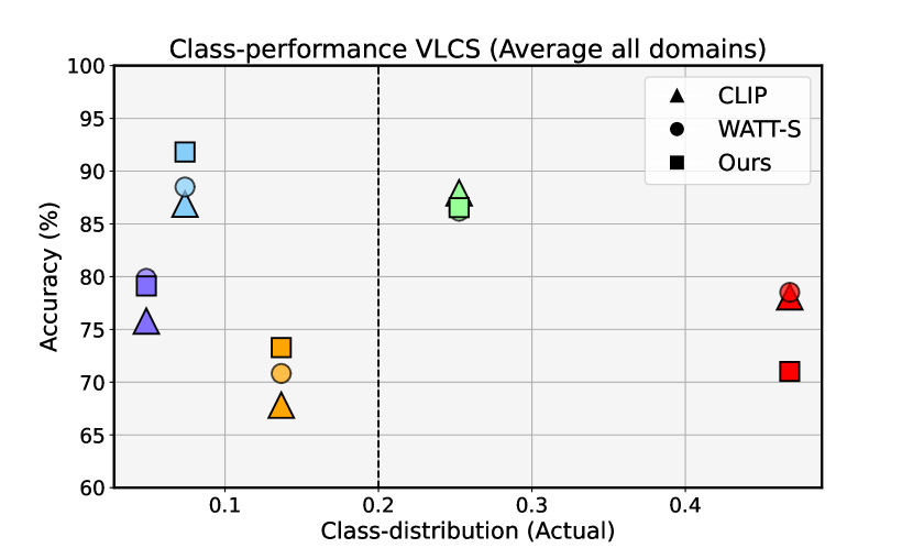
Figure 1: Further exploration on the VLCS dataset, averaged over the different sub-domains. Classes are represented by colours (Person, Chair, Bird, Car, Dog). The vertical line represents the uniform class distribution scenario for VLCS, i.e., 20%.

4.3 Ablation studies

Impact of each component.  In Figure 2, we empirically validate the benefit of each component in CLIP-OT design. Each configuration is detailed in Appendix C.1. First, we can observe that computing the code $Q^{*}_{m}$ from each template $m$ (Eq. (9)) and averaging those to obtain the final predictions consistently improves over zero-shot CLIP. It is noteworthy to stress that, while this performance is far from state-of-the-art approaches, this strategy is training-free, not requiring additional computational complexity due to gradient descent updates. Next, Average Template employs the pseudo-codes computed in the previous version to minimize the cross-entropy in Eq. (3). Furthermore, the prediction for the $i$-th image, $\mathbf{p}_{i}$, is computed with the average template for the class $k$, i.e., $\mathbf{t}_{k}$. This shows that leveraging the obtained pseudo-codes to refine the model leads to a performance improvement, which is consistent across all datasets. Last, we introduce the novel knowledge distillation strategy proposed in this work, where distinct templates are used to get multiple pseudo-codes and guide the model training, i.e., CLIP-OT. Its substantial performance gains are especially notable in the most challenging scenarios, e.g., CIFAR-100C.

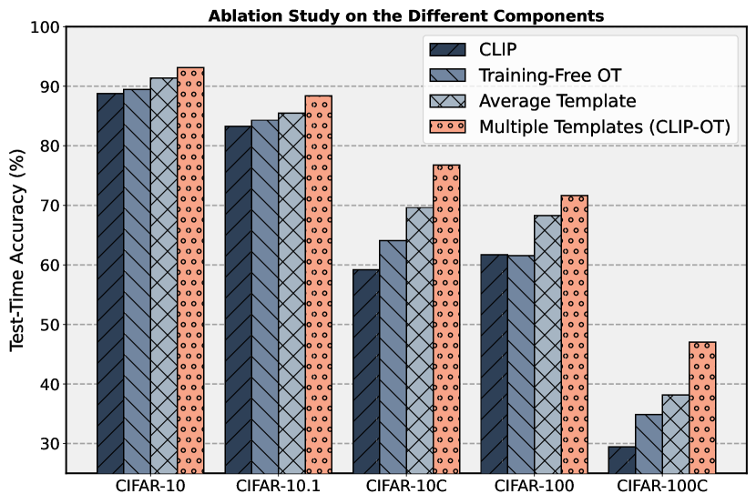
Figure 2: Ablation on each component across multiple datasets. Different results come from adding each element of the proposed formulation. The numerical values are provided in Appendix C.

Table 5: Accuracy (%) of CLIP-OT with varying numbers of templates (see Appendix A) on CIFAR-10.

$\#$ Templates	1	2	3	4	5	6	7	8
CIFAR-10	91.59	92.16	92.46	92.69	92.88	93.04	93.14	93.14
CIFAR-100	68.36	69.46	70.08	70.56	70.90	71.15	71.38	71.34
Tiny-ImageNet	60.62	61.73	62.32	62.69	62.95	63.16	63.20	63.11

On the impact of multiple templates.  We now assess how the performance evolves as the number of templates increases (Table 5). Concretely, we trained our model multiple times, varying the number of templates $N\in\{1,\dots,8\}$. For each $N$, the average accuracy over all template combinations was computed, leading to 256 experiments per dataset. Results from this experiment show that CLIP-OT performance consistently increases with the number of templates. This showcases how leveraging individually multiple templates can extract richer information to adapt CLIP at test time.

Do observations hold across backbones?  Table 6 reports the performance across different datasets when ViT-B/16 is employed as the visual encoder of CLIP. These results demonstrate that CLIP-OT is model agnostic, as its superiority is consistently maintained across different backbones.

Table 6: Quantitative results with ViT-B/16 as backbone across different datasets and baselines.

Dataset	CLIP	TENT	TPT	CLIPArTT	WATT-S	CLIP-OT
CIFAR-10	89.25	92.75	89.90	92.61	91.97	94.69
CIFAR-10.1	84.00	88.52	83.75	88.72	88.10	89.25
CIFAR-10C	60.15	68.00	59.75	73.22	76.22	80.11
CIFAR-100	64.76	71.73	67.15	71.34	72.85	74.06
CIFAR-100C	32.01	37.90	33.73	40.08	48.95	51.24
TinyImageNet	58.12	63.59	63.87	64.73	66.05	66.34
TinyImageNet-C	20.92	29.78	26.96	32.90	31.66	37.69

Computational analysis.  Table 7 introduces figures of merit for relevant baselines and the proposed CLIP-OT for several datasets with an increasing complexity, i.e., number of categories. First, it is worth noting that all methods require similar GPU resources for training since they update the same layers in the CLIP encoder. However, they substantially differ in total runtimes. In this focus, CLIP-OT archives homogeneous figures for all datasets, whatever their complexity. In contrast, the recent state-of-the-art WATT-S constantly increases the required runtime with the number of classes, driven by its iterative nature on the multiple template evaluations and weight averaging during inference. In contrast, CLIP-OT does not require such a burden since this information is properly distilled during the adaptation stage. This combination of speed and consistency establishes CLIP-OT as the most scalable and effective method, providing runtimes $\times$12 and $\times$26 faster than TENT and WATT-S, respectively, for the most complex dataset, i.e., Tiny-ImageNet.

Table 7: Computational efficiency of CLIP TTA methods. Results for an average input batch.

Dataset	Method	Runtime	GPU Memory
		(seconds)	(Gb)
CIFAR-10	TENT	1.08	4.59
	WATT-S	8.60	4.59
	CLIP-OT	0.62	4.59
CIFAR-100	TENT	4.14	4.59
	WATT-S	11.83	4.59
	CLIP-OT	0.62	4.50
Tiny-ImageNet	TENT	7.67	4.59
	WATT-S	15.96	4.59
	CLIP-OT	0.62	4.50

5 Conclusions

In this work, we have presented a novel approach for Test-Time Adaptation in vision-language models. In particular, CLIP-OT generates pseudo-labels for test samples using multiple, generic class templates, optimizing a label assignment problem solved with Optimal Transport. This strategy yields state-of-the-art results compared to recent works in several benchmarks, yet being a more efficient solution.

Limitations.  Even though CLIP-OT outperforms by a substantial margin very recent CLIP TTA methods across most datasets, its behavior for a very extremely imbalanced dataset, i.e., VLCS, is not optimal, driven by one over-represented class. On the other hand, CLIP-OT appears to be a promising option for enhancing adaptation on under-represented concepts. It is worth noting that all recent methods struggle with such imbalance tasks, marginally (if so) outperforming base CLIP predictions, which suggests future attention should be paid to this scenario.

Acknowledgments  This work was funded by the Natural Sciences and Engineering Research Council of Canada (NSERC). We also thank Calcul Quebec and Compute Canada.

Supplementary Material

Appendix A Templates Used

In the experimental setup, several predefined text templates from CLIP [10] to evaluate the adaptability and performance of the proposed model were used. These templates are designed to generalize across different contexts and image types, allowing for a robust assessment of the model’s capabilities in handling diverse visual and textual representations. In Table 8, we provide the list of templates used in our experiments. Each template includes a placeholder , which is dynamically replaced with the class name during the generation of text prompts. Note that, for the sake of fairness with prior literature, the templates are the same as the ones employed in WATT [29].

Table 8: The different templates used during the experiments.

	Template
1:	“a photo of a {class $k$}”
2:	“itap of a {class $k$}”
3:	“a bad photo of the {class $k$}”
4:	“a origami {class $k$}”
5:	“a photo of the large {class $k$}”
6:	“a {class $k$} in a video game”
7:	“art of the {class $k$}”
8:	“a photo of the small {class $k$}”

Appendix B Additional details on the datasets

CIFAR-10.1 introduces a natural shift from CIFAR-10, whereas CIFAR-10-C and CIFAR-100-C are augmented with 15 different corruptions across 5 severity levels (each containing 10,000 images), leading to 75 corruption scenarios commonly employed in domain shift problems. These datasets are critical for evaluating how well models can generalize to real-world variations and noise that are not present in the training set. Tiny-ImageNet is a downsized version of the original ImageNet dataset, providing a more accessible challenge with 200 classes. It serves as a useful benchmark for lightweight models and for educational purposes, making it easier to implement and experiment with domain adaptation techniques. Tiny-ImageNet-C further extends Tiny-ImageNet by incorporating various common corruptions, similar to CIFAR-10-C and CIFAR-100-C. This dataset is instrumental for testing the robustness of models against a variety of distortions in a more manageable setting. To assess the performance on class imbalanced datasets, we employ several datasets from Domainbed (PACS, VLCS, OfficeHome, VisDA-C) that are often utilized for benchmarking domain adaptation algorithms. Each dataset presents unique domain shift challenges and diverse visual categories, allowing for a comprehensive evaluation of a model’s ability to generalize across different environments under varying class distributions.

Furthermore, in the main paper we stated that the lower performance obtained by our approach in VLCS may stem from the imbalanced nature of its class distribution. Table 9 summarizes the class statistics of the VLCS dataset, highlighting its large class imbalance across subdomains.

Table 9: Summary of the class statistics across sub-domains for the VLCS dataset.

Domain	# of samples (Highest)	# of samples (Lowest)	Ratio
Caltech	809	62	13.0
LabelMe	1124	39	28.9
SUN	1175	19	61.9
Pascal	1394	307	4.6

Appendix C Additional details of the ablation studies

C.1 Configuration: Baselines

In this section, we detail the configurations used to assess the impact of each main component of our approach, which we refer to Training-free OT and CLIP-OT with Average Template. Note that, in short, Training-free OT motivates the use of the pseudo-codes $\mathbf{Q}^{*}$ over the CLIP baseline, whereas CLIP-OT with Average Template includes these pseudo-codes to fine-tune the model. Furthermore, we want to highlight that the later does not fully leverage multiple individual templates, which is introduced in our proposed CLIP-OT model. A more detailed description follows. Given a batch of test images, Training-free OT (Algorithm 2) computes pseudo-codes for each text template, which are later averaged to produce a final prediction. On the other hand, CLIP-OT with Average Template (Algorithm 3) utilizes the averaged pseudo-codes (obtained by Training-free OT) to refine the visual encoder. More concretely, at each batch, the average pseudo-codes $\tilde{\mathbf{Q}}$ supervise the predictions of the test images produced by the model. These predictions are obtained by resorting to Eq. (1), where the average class embedding $\mathbf{t}_{k}$ is used, together with the visual embeddings of the test images, $\mathbf{Z}$. Differences between the pseudo-codes and the predictions are minimized via a cross-entropy loss, whose gradients are used to update the layer norm parameters of the model. Then, once the model is updated, we can do the final inference for the test images.

Algorithm 2 Training-free OT.

1:input: test dataset $\mathcal{X}=\{\mathbf{x}_{n}\}$ (images), text templates $\mathcal{T}$ (class descriptions), visual and text encoders ($\boldsymbol{\theta}$, $\phi$). // Split $\mathcal{X}$ into $B$ batches of size $B_{s}$. // Compute $K\times M$ text prototypes ($\boldsymbol{\phi}(\mathcal{T}),\forall m,k)$.

2:$\mathbf{T}\in\mathbb{R}^{d\times K\times M}=\left[\mathbf{t}_{km}\right]_{k=1,\dots,K,m=1,\dots,M}$

3:for sampled minibatch $\{\mathbf{x}_{i}\}_{i=1}^{B_{s}}$ do

4:       for each template $m$ in a random permutation of $\{1,2,\dots,M\}$ do   // Step 1: Generation of pseudo-codes $Q^{*}_{m}$.

5:             $\mathbf{T}_{m}\in\mathbb{R}^{d\times K}$ // class text embeddings for $m$.

6:             $\mathbf{Z}=[\mathbf{z}_{1},\dots,\mathbf{z}_{B_{s}}]$ // visual features ($\boldsymbol{\theta}_{\text{LN}}^{(m-1)}$).

7:             Compute pseudo-codes $\mathbf{Q}^{*}_{m}$ // Eq. (9).

8:       end for // Inference (for all images in the batch).

9:       $\mathbf{P}=[\mathbf{p}_{1},\dots,\mathbf{p}_{B_{s}}]$ // predict: $\mathbf{p}_{i}=\frac{1}{M}\sum_{m=1}^{M}\mathbf{q}_{im}$.

10:end for

Algorithm 3 CLIP-OT with Average Template.

1:input: test dataset $\mathcal{X}=\{\mathbf{x}_{n}\}$ (images), text templates $\mathcal{T}$ (class descriptions), visual and text encoders ($\boldsymbol{\theta}$, $\phi$). // Split $\mathcal{X}$ into $B$ batches of size $B_{s}$. // Compute $K\times M$ text prototypes ($\boldsymbol{\phi}(\mathcal{T}),\forall m,k)$.

2:$\mathbf{T}\in\mathbb{R}^{d\times K\times M}=\left[\mathbf{t}_{km}\right]_{k=1,\dots,K,m=1,\dots,M}$

3:for sampled minibatch $\{\mathbf{x}_{i}\}_{i=1}^{B_{s}}$ do // 1 - Adaptation

4:       for each template $m$ in a random permutation of $\{1,2,\dots,M\}$ do   // Step 1: Generation of pseudo-codes $Q^{*}_{m}$.

5:             $\mathbf{T}_{m}\in\mathbb{R}^{d\times K}$ // class text embeddings for $m$.

6:             $\mathbf{Z}=[\mathbf{z}_{1},\dots,\mathbf{z}_{B_{s}}]$ // visual features ($\boldsymbol{\theta}_{\text{LN}}^{(m-1)}$).

7:             Compute pseudo-codes $\mathbf{Q}^{*}_{m}$ // Eq. (9).

8:       end for // Step 2: Compute average pseudo-codes and refine the encoder.

9:       $\tilde{\mathbf{Q}}=\frac{1}{M}\sum_{m=1}^{M}\mathbf{Q}^{*}_{m}$ // average pseudo-codes.

10:       $\mathbf{t}_{k}=\frac{1}{M}\sum_{m=1}^{M}\mathbf{t}_{km}$ // average class text embeddings over all templates.

11:       $\mathbf{P}=[\mathbf{p}_{1},\dots,\mathbf{p}_{B_{s}}]$ // predict with $\mathbf{t}_{k},\forall k$, Eq. (1).

12:       Min. cross-entropy loss between $\mathbf{P}$ and $\tilde{\mathbf{Q}}$ // Eq. (3).

13:       $\theta_{\text{LN}}^{(t)}\rightarrow\theta_{\text{LN}}^{(t+1)}$ // update layer norm. // 2 - Inference (for all images in the batch).

14:       $\mathbf{Z}=[\mathbf{z}_{1},\dots,\mathbf{z}_{B_{s}}]$ // visual features (with $\boldsymbol{\theta}_{\text{LN}}^{(m)}$).

15:       $\mathbf{P}=[\mathbf{p}_{1},\dots,\mathbf{p}_{B_{s}}]$ // predict with $\mathbf{t}_{k},\forall k$, Eq. (1).

16:end for

C.2 Extended numerical values

We further substantiate the findings presented in Figure 2 by providing detailed quantitative results in Tables 10 and 11. The tables showcase a comprehensive performance comparison of the impact of the different components of our approach, which empirically motivate our model. These results are reported for different corruption benchmarks on the CIFAR-10, CIFAR-10.1 CIFAR-10C, CIFAR-100 and CIFAR-100C datasets, respectively, using a ViT-B/32 backbone.

Table 10: Numerical Analysis for CIFAR-10, CIFAR-10.1 and CIFAR-10-C datasets as shown in Figure 2.

Dataset	CLIP	Training-Free OT	Avg. Template	CLIP-OT
CIFAR-10	88.74	89.44	91.40	93.15
CIFAR-10.1	83.25	84.30	85.50	88.37
Gaussian Noise	35.27	46.68	54.68	64.85
Shot Noise	39.67	49.84	57.13	67.34
Impulse Noise	42.61	47.18	52.72	62.27
Defocus Blur	69.76	73.22	77.84	82.09
Glass Blur	42.40	50.09	56.88	68.07
Motion Blur	63.97	70.15	74.81	81.30
Zoom Blur	69.83	74.19	77.99	83.13
Snow	71.78	73.93	78.41	83.71
Frost	72.86	75.66	79.31	83.40
Fog	67.04	69.28	75.54	82.56
Brightness	81.87	82.90	86.87	89.90
Contrast	64.37	67.30	75.30	84.86
Elastic Transform	60.83	64.06	69.54	76.08
Pixelate	50.53	56.65	62.91	76.25
JPEG Compression	55.48	59.75	64.31	70.03
Mean	59.22	64.05	69.62	77.06

Table 11: Numerical Analysis for CIFAR-100 and CIFAR-100-C datasets as shown in Figure 2.

Corruption	CLIP	Training-Free OT	Avg. Template	CLIP-OT
CIFAR-100	61.68	61.55	68.26	71.68
Gaussian Noise	14.80	21.26	23.29	33.43
Shot Noise	16.03	22.98	25.15	35.60
Impulse Noise	13.85	22.27	22.14	30.94
Defocus Blur	36.74	41.40	46.84	53.87
Glass Blur	14.19	22.47	23.60	35.26
Motion Blur	36.14	40.71	44.41	52.77
Zoom Blur	40.24	45.14	49.97	56.71
Snow	38.95	44.14	46.73	54.30
Frost	40.56	45.03	47.85	54.92
Fog	38.00	40.00	45.45	53.57
Brightness	48.18	51.26	57.22	64.43
Contrast	29.53	33.69	41.16	55.01
Elastic Transform	26.33	33.02	34.85	43.79
Pixelate	21.98	27.72	30.13	44.51
JPEG Compression	25.91	31.69	33.80	40.83
Mean	29.43	34.85	38.17	47.33

Appendix D Comparison to OT-VP

The very recent OT-VP [45] has presented a solution integrating optimal transport for test-time adaptation. Nevertheless, it presents several fundamental differences with our work. First, OT-VP involves learning a universal visual prompt for the target domain, for which an optimal transport distance is optimized. Thus, optimal transport is used for a different task. Second, OT-VP is tailored to only visual models, not being capable of leveraging the valuable information found on the text modality. And third, the adaptation scenario strongly differs from our setting. In particular, OT-VP first fine-tunes the pre-trained model (pre-trained on ImageNet-1k) to a subdomain (e.g., PACS) with labeled data, to later adapt at test-time to the other subdomains (e.g., VLCS and OfficeHome). While this strategy can be done in a single-source setting, OT-VP also evaluates the performance when multiple domains are used as the source (e.g., supervised adaptation on PACS and VLCS), and only one left out for testing, referred to as Multi-Source in Table 12. In contrast, we follow the protocol of recent literature of CLIP test-time adaptation, where CLIP is directly exposed to the unsupervised test data points, without intermediate adaptation steps. To expand the extent of our empirical validation, we compare our approach to OT-VP [45] whose results are reported in Table 12. To ensure a rigorous comparison, we use the same visual encoder as the backbone used in OT-VP and other prior models, i.e., ViT-B/16.

Table 12: Performance comparison to [45] across PACS, VLCS, and OfficeHome datasets. Best results highlighted in bold, whereas ${}_{{\textbf{{\color[rgb]{0.5,0.5,0.5}value}}}}$ indicates the difference wrt OT-VP in both single (first value) and multi (second value) source scenarios.

Method	PACS	VLCS	OfficeHome	Avg.
First Setting : Single Source
OT-VP-B${}_{\textit{WACV'25}}$	69.8	65.2	66.9	67.3
OT-VP${}_{\textit{WACV'25}}$	73.5	68.4	68.1	70.0
Second Setting : Multi Source
OT-VP-B${}_{\textit{WACV'25}}$	87.3	80.2	74.3	80.6
OT-VP${}_{\textit{WACV'25}}$	87.7	80.9	75.1	81.2
Our setting: No specific source
CLIP-OT (Ours)	96.9${}_{{\textbf{{\color[rgb]{0.5,0.5,0.5}+23.4/+9.2}}}}$	80.2${}_{{\textbf{{\color[rgb]{0.5,0.5,0.5}+11.8/-0.7}}}}$	83.4${}_{{\textbf{{\color[rgb]{0.5,0.5,0.5}+15.3/+8.3}}}}$	86.8${}_{{\textbf{{\color[rgb]{0.5,0.5,0.5}+16.8/+5.6}}}}$

Appendix E Additional Details on Epsilon ($\epsilon$)

In the main paper, we stated that $\epsilon$, the entropic constraint weight in Eq. 7 was set to $\epsilon=0.7$ based on preliminary experiments. However, here in the appendix, we explore the sensitivity of the model to different values of $\epsilon$ to assess its impact on accuracy under various corruptions and datasets. As shown in Table 13, we experimented with $\epsilon$ values of 0.3, 0.5, 0.7 and 0.9 across CIFAR-10C and CIFAR-100C datasets. Further, we show the values for CIFAR-10 and CIFAR-100 datasets along with averaged performance over corruptions in the Figure 3.

Table 13: Mean Accuracy for CIFAR-10 and CIFAR-100 under Different Corruptions and Epsilon Values

Corruption	CIFAR-10				CIFAR-100
	0.3	0.5	0.7	0.9	0.3	0.5	0.7	0.9
Original	91.15	93.01	93.15	92.81	62.26	70.95	71.62	71.01
Gaussian Noise	56.16	63.65	64.43	65.26	13.74	32.03	33.2	32.44
Shot Noise	57.53	66.29	66.27	67.4	15.62	34.69	35.33	35.46
Impulse Noise	54.27	61.22	61.84	62.42	19.44	29.94	30.99	30.36
Defocus Blur	76.27	81.33	82.1	82.49	39.16	52.77	54.16	53.32
Glass Blur	57.63	66.75	67.55	67.96	17.06	34.46	35.24	34.89
Motion Blur	71.99	80.11	81.31	80.9	36.59	51.33	52.67	51.62
Zoom Blur	76.24	82.54	83.11	83.46	42.58	55.53	56.93	56.13
Snow	78.59	83.39	82.99	83.56	40.91	53.54	54.06	54.12
Frost	78.92	82.67	82.93	83.41	40.98	54.1	54.93	54.37
Fog	75.75	81.64	81.9	82.47	40.76	52.69	53.6	53.12
Brightness	85.97	89.59	89.72	89.71	48.31	63.27	64.87	63.57
Contrast	70.38	83.55	84.53	84.6	32.09	53.61	55.39	54.41
Elastic Transform	69.17	75.42	75.67	76.09	27.78	42.69	43.78	43.01
Pixelate	61.31	74.57	76.51	76.08	22.79	42.64	44.96	43.18
JPEG Compression	66.02	69.42	70.46	70.03	30.16	40.16	41.02	40.67
Mean	70.46	76.14	76.75	77.06	31.20	46.23	47.41	46.71

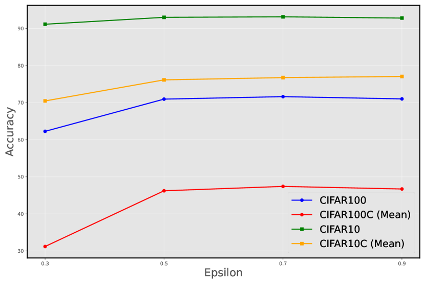
Figure 3: Ablation on epsilon values across multiple datasets.

We can observe that higher $\epsilon$ values (0.7 and 0.9) generally led to improved stability and performance, which can be attributed to stronger regularization introduced by higher entropic constraints, which prevents degenerate solutions during Sinkhorn normalization. While smaller $\epsilon$ values sometimes performed better under mild corruptions, they exhibited significant instability during Sinkhorn normalization. In several cases, the $\mathbf{Q}$ matrix became NaN, especially under high noise corruptions, rendering the adaptation process unusable. This behavior can be attributed to insufficient regularization, causing numerical instabilities during iterative updates. The chosen value ($\epsilon=0.7$) strikes a balance between stability and performance, yielding robust results across both clean and corrupted datasets.

Appendix F Discussion on the Two Hyperparameters of WATT and Motivation for CLIP-OT

WATT [29] introduces two key hyperparameters: $L$ (number of adaptation iterations for each text embedding) and $M$ (number of repetitions of the weight averaging process). While these hyperparameters play an essential role in improving WATT’s adaptation capabilities, they introduce significant computational and scalability challenges, particularly as the number of classes grows. The iterative nature of $L$ requires multiple forward and backward passes for every template, leading to substantial runtime overhead, especially for datasets with many classes like Tiny-ImageNet. Additionally, higher $L$ values, while effective for complex corruptions, risk overfitting to noisy pseudo-labels, while lower $L$ values may lead to under-adaptation. Similarly, $M$ stabilizes adaptation through repeated weight averaging, but its effectiveness diminishes beyond a certain point, with larger values providing negligible performance improvements while exponentially increasing runtime. This dependence on repeated updates for each class and template becomes especially prohibitive for datasets with a large number of classes, as demonstrated in Table 7, where runtime increases from CIFAR-10 (10 classes) to Tiny-ImageNet (200 classes).

These limitations motivate our proposed approach, CLIP-OT , which simplifies and optimizes the adaptation process, achieving robust performance without the drawbacks associated with $L$ and $M$. CLIP-OT eliminates these limitations by leveraging the Sinkhorn algorithm for single-pass optimization and precomputing averaged class embeddings, removing the need for iterative updates and weight averaging. This not only drastically reduces computational overhead but also ensures scalable, robust adaptation across diverse corruption levels and datasets, offering a practical alternative to WATT’s hyperparameter-dependent framework.

Appendix G Further results on other backbones

In this section, we present additional experimental results leveraging different backbone architectures to evaluate the robustness and generalizability of our proposed method. Specifically, we analyze the performance of CLIP models with ViT-B/16 and ViT-L/14 backbones across various datasets, including CIFAR, Tiny-ImageNet and their corruptions. These experiments validate our approach across diverse settings and highlight its adaptability to challenging domain shifts.

Table 14 details the performance of CLIP-OT with the ViT-B/16 backbone on CIFAR-10, CIFAR-10.1, and CIFAR-10-C datasets. Our proposed method demonstrates consistent improvements across both clean and corrupted data, outperforming baseline methods such as CLIP, TENT, and TPT. Similarly for ViT-L/14 backbone on these datasets, we obtain similar gains as illustrated in Table 15. Table 16 extends the evaluation to CIFAR-100 and CIFAR-100-C, demonstrating the effectiveness of our method on more complex datasets with larger label spaces. Using CLIP with the ViT-B/16 backbone, our approach achieves the highest average accuracy, with substantial improvements under corruptions such as Glass Blur ($+5.30\%$) and Contrast ($+6.23\%$). We also evaluate these datasets with backbone ViT/L-14 in Table 17.

For Tiny-ImageNet and its corrupted version, Tiny-ImageNet-C, Table 18 and Table 19 provides a detailed breakdown. On datasets with higher complexity and larger label spaces, such as Tiny-ImageNet and Tiny-ImageNet-C (Table 18), CLIP-OT exhibits substantial gains, consistent with the main paper’s observations. Specifically, our method improves over WATT-S by over 6% on average across Tiny-ImageNet-C corruptions, showcasing its scalability to more challenging scenarios.

G.1 Tiny-Imagenet Experiments

We report the mean and standard deviation over Tiny-Imagenet related experiments (Table 3, main paper) in Table 20.

Table 14: Accuracy (%) on CIFAR-10, CIFAR-10.1, and CIFAR-10-C datasets with ViT-B/16 as visual encoder.

Dataset	CLIP ICLR’21	TENT ICLR’21	TPT NeurIPS’22	CLIPArTT Arxiv’24	WATT-P NeurIPS’24	WATT-S NeurIPS’24	CLIP-OT Ours
CIFAR-10	89.25	92.75 $\pm$0.17	89.80 $\pm$0.05	92.61 $\pm$0.05	92.31 $\pm$0.10	91.97 $\pm$0.03	94.69 $\pm$0.18
CIFAR-10.1	84.00	88.52 $\pm$0.33	83.75 $\pm$0.21	88.72 $\pm$0.33	87.90 $\pm$0.11	88.10 $\pm$0.08	89.25 $\pm$0.08
Gaussian Noise	37.75	31.04 $\pm$0.38	35.35 $\pm$0.15	60.89 $\pm$0.26	63.10 $\pm$0.12	65.57 $\pm$0.22	68.50 $\pm$0.19
Shot Noise	41.10	40.54 $\pm$0.41	41.03 $\pm$0.19	65.19 $\pm$0.21	66.31 $\pm$0.10	68.67 $\pm$0.37	71.24 $\pm$0.22
Impulse Noise	51.71	58.03 $\pm$0.16	54.86 $\pm$0.07	67.55 $\pm$0.09	69.62 $\pm$0.12	70.39 $\pm$0.11	76.97 $\pm$0.17
Defocus Blur	70.07	77.57 $\pm$0.03	70.29 $\pm$0.02	78.92 $\pm$0.12	79.64 $\pm$0.08	79.90 $\pm$0.07	83.33 $\pm$0.09
Glass Blur	42.24	47.16 $\pm$0.05	37.86 $\pm$0.17	57.18 $\pm$0.20	58.98 $\pm$0.12	61.62 $\pm$0.21	68.33 $\pm$0.20
Motion Blur	65.81	76.16 $\pm$0.05	67.43 $\pm$0.11	76.59 $\pm$0.06	78.32 $\pm$0.16	79.02 $\pm$0.07	83.13 $\pm$0.10
Zoom Blur	72.50	79.64 $\pm$0.12	72.91 $\pm$0.02	79.62 $\pm$0.11	80.67 $\pm$0.07	81.10 $\pm$0.08	85.35 $\pm$0.11
Snow	73.23	81.68 $\pm$0.03	72.98 $\pm$0.32	81.13 $\pm$0.29	81.99 $\pm$0.10	82.54 $\pm$0.18	86.65 $\pm$0.12
Frost	76.52	83.22 $\pm$0.05	75.87 $\pm$0.16	81.24 $\pm$0.08	83.41 $\pm$0.16	83.46 $\pm$0.15	86.37 $\pm$0.09
Fog	68.35	80.78 $\pm$0.15	69.13 $\pm$0.27	78.47 $\pm$0.19	81.36 $\pm$0.12	81.88 $\pm$0.12	85.60 $\pm$0.24
Brightness	83.36	89.85 $\pm$0.11	83.67 $\pm$0.14	88.66 $\pm$0.15	89.06 $\pm$0.05	89.10 $\pm$0.14	92.64 $\pm$0.11
Contrast	61.90	79.24 $\pm$0.19	62.16 $\pm$0.06	75.15 $\pm$0.07	81.57 $\pm$0.23	83.79 $\pm$0.12	86.92 $\pm$0.18
Elastic Transform	53.16	62.54 $\pm$0.08	51.26 $\pm$0.23	69.49 $\pm$0.08	69.14 $\pm$0.09	70.93 $\pm$0.20	75.18 $\pm$0.14
Pixelate	48.48	67.08 $\pm$0.24	44.65 $\pm$0.21	71.80 $\pm$0.16	73.38 $\pm$0.29	75.67 $\pm$0.32	78.73 $\pm$0.30
JPEG Compression	56.05	65.42 $\pm$0.05	56.73 $\pm$0.07	66.42 $\pm$0.25	69.02 $\pm$0.10	69.65 $\pm$0.23	72.65 $\pm$0.18
Mean	60.15	68.00	59.75	73.22	75.04	76.22	80.11

Table 15: Accuracy (%) on CIFAR-10, CIFAR-10.1, and CIFAR-10-C datasets with ViT-L/14 as visual encoder.

Dataset	CLIP ICLR’21	TENT ICLR’21	TPT NeurIPS’22	CLIPArTT Arxiv’24	WATT-P NeurIPS’24	WATT-S NeurIPS’24	CLIP-OT Ours
CIFAR-10	95.36	96.13 $\pm$0.06	95.18 $\pm$0.02	95.16 $\pm$0.03	95.91 $\pm$0.10	95.71 $\pm$0.03	97.61 $\pm$0.03
CIFAR-10.1	91.20	92.22 $\pm$0.25	91.32 $\pm$0.12	91.02 $\pm$0.02	92.97 $\pm$0.13	92.10 $\pm$0.33	93.45 $\pm$0.30
Gaussian Noise	64.64	68.87 $\pm$0.20	64.44 $\pm$0.11	70.04 $\pm$0.31	72.81 $\pm$0.09	72.73 $\pm$0.03	80.47 $\pm$0.26
Shot Noise	67.82	71.95 $\pm$0.06	66.81 $\pm$0.19	71.44 $\pm$0.16	74.45 $\pm$0.16	74.60 $\pm$0.03	82.64 $\pm$0.29
Impulse Noise	78.21	80.22 $\pm$0.19	76.46 $\pm$0.17	79.42 $\pm$0.15	81.36 $\pm$0.09	80.95 $\pm$0.15	87.80 $\pm$0.15
Defocus Blur	80.73	83.10 $\pm$0.03	79.01 $\pm$0.23	81.75 $\pm$0.19	83.20 $\pm$0.10	83.15 $\pm$0.18	90.33 $\pm$0.12
Glass Blur	50.29	57.12 $\pm$0.07	49.64 $\pm$0.23	58.13 $\pm$0.23	61.51 $\pm$0.07	62.35 $\pm$0.15	77.72 $\pm$0.31
Motion Blur	80.75	82.69 $\pm$0.11	78.85 $\pm$0.04	80.76 $\pm$0.12	82.60 $\pm$0.13	82.61 $\pm$0.12	88.93 $\pm$0.17
Zoom Blur	82.75	84.91 $\pm$0.08	82.32 $\pm$0.13	83.39 $\pm$0.05	85.76 $\pm$0.06	85.44 $\pm$0.13	91.69 $\pm$0.13
Snow	83.01	85.99 $\pm$0.11	82.69 $\pm$0.10	84.48 $\pm$0.07	84.91 $\pm$0.13	85.61 $\pm$0.15	91.56 $\pm$0.11
Frost	84.90	87.15 $\pm$0.12	84.63 $\pm$0.08	85.21 $\pm$0.06	87.17 $\pm$0.13	86.88 $\pm$0.04	91.43 $\pm$0.12
Fog	78.44	81.30 $\pm$0.07	77.56 $\pm$0.17	79.27 $\pm$0.07	81.80 $\pm$0.11	81.79 $\pm$0.09	90.82 $\pm$0.11
Brightness	91.67	93.07 $\pm$0.04	90.94 $\pm$0.04	91.87 $\pm$0.09	92.78 $\pm$0.05	92.59 $\pm$0.16	95.86 $\pm$0.00
Contrast	84.20	87.93 $\pm$0.04	82.88 $\pm$0.09	86.19 $\pm$0.06	87.54 $\pm$0.12	87.38 $\pm$0.02	94.53 $\pm$0.08
Elastic Transform	65.45	69.96 $\pm$0.12	64.81 $\pm$0.14	67.43 $\pm$0.24	71.19 $\pm$0.07	71.25 $\pm$0.09	82.16 $\pm$0.23
Pixelate	75.10	77.89 $\pm$0.05	72.92 $\pm$0.12	77.11 $\pm$0.10	77.88 $\pm$0.13	77.67 $\pm$0.16	87.13 $\pm$0.16
JPEG Compression	72.58	75.49 $\pm$0.07	71.18 $\pm$0.19	74.46 $\pm$0.11	75.88 $\pm$0.16	75.84 $\pm$0.18	82.60 $\pm$0.18
Mean	76.04	79.18	75.01	78.06	80.05	80.06	86.35

Table 16: Accuracy (%) on CIFAR-100 and CIFAR-100-C datasets with ViT-B/16 as visual encoder.

Dataset	CLIP ICLR’21	TENT ICLR’21	TPT NeurIPS’22	CLIPArTT Arxiv’24	WATT-P NeurIPS’24	WATT-S NeurIPS’24	CLIP-OT Ours
CIFAR-100	64.76	71.73 $\pm$0.14	67.15 $\pm$0.23	71.34 $\pm$0.07	72.98 $\pm$0.07	72.85 $\pm$0.15	74.07 $\pm$0.20
Gaussian Noise	15.88	12.28 $\pm$0.20	15.43 $\pm$0.03	19.01 $\pm$0.24	34.23 $\pm$0.03	35.95 $\pm$0.27	38.80 $\pm$0.51
Shot Noise	17.49	15.07 $\pm$0.21	16.88 $\pm$0.07	20.27 $\pm$0.21	36.68 $\pm$0.10	37.96 $\pm$0.15	40.89 $\pm$0.10
Impulse Noise	21.43	13.13 $\pm$0.16	22.12 $\pm$0.15	17.66 $\pm$0.10	43.17 $\pm$0.35	44.62 $\pm$0.20	46.39 $\pm$0.17
Defocus Blur	40.10	50.35 $\pm$0.03	41.08 $\pm$0.22	49.86 $\pm$0.13	53.13 $\pm$0.12	53.80 $\pm$0.12	55.50 $\pm$0.24
Glass Blur	13.48	04.84 $\pm$0.14	18.43 $\pm$0.15	18.34 $\pm$0.31	32.53 $\pm$0.03	33.39 $\pm$0.11	37.89 $\pm$0.68
Motion Blur	39.82	49.85 $\pm$0.37	40.85 $\pm$0.26	50.00 $\pm$0.09	51.63 $\pm$0.06	52.72 $\pm$0.30	55.10 $\pm$0.28
Zoom Blur	45.45	54.76 $\pm$0.04	46.77 $\pm$0.06	54.13 $\pm$0.08	56.81 $\pm$0.11	57.51 $\pm$0.09	58.77 $\pm$0.33
Snow	42.77	52.38 $\pm$0.18	47.24 $\pm$0.18	52.80 $\pm$0.27	56.04 $\pm$0.06	56.73 $\pm$0.27	57.84 $\pm$0.13
Frost	45.39	51.66 $\pm$0.04	48.61 $\pm$0.14	49.56 $\pm$0.08	56.00 $\pm$0.11	56.48 $\pm$0.34	58.09 $\pm$0.04
Fog	38.98	50.74 $\pm$0.14	39.92 $\pm$0.16	49.92 $\pm$0.11	52.88 $\pm$0.33	53.83 $\pm$0.19	55.68 $\pm$0.38
Brightness	52.55	64.26 $\pm$0.09	55.83 $\pm$0.10	63.76 $\pm$0.13	65.58 $\pm$0.07	66.67 $\pm$0.19	67.76 $\pm$0.21
Contrast	33.32	48.69 $\pm$0.08	33.13 $\pm$0.16	47.86 $\pm$0.02	52.90 $\pm$0.06	55.06 $\pm$0.15	58.29 $\pm$0.51
Elastic Transform	24.39	33.56 $\pm$0.28	27.36 $\pm$0.10	32.93 $\pm$0.23	39.82 $\pm$0.21	40.37 $\pm$0.26	44.32 $\pm$0.18
Pixelate	21.89	36.20 $\pm$0.28	21.26 $\pm$0.10	39.49 $\pm$0.21	45.10 $\pm$0.06	47.02 $\pm$0.04	49.46 $\pm$0.17
JPEG Compression	27.21	30.80 $\pm$0.05	30.97 $\pm$0.10	35.56 $\pm$0.23	41.43 $\pm$0.18	42.13 $\pm$0.21	43.87 $\pm$0.23
Mean	32.01	37.90	33.73	40.08	47.86	48.95	51.24

Table 17: Accuracy (%) on CIFAR-100 and CIFAR-100-C datasets with ViT-L/14 as visual encoder.

Dataset	CLIP ICLR’21	TENT ICLR’21	TPT NeurIPS’22	CLIPArTT Arxiv’24	WATT-P NeurIPS’24	WATT-S NeurIPS’24	CLIP-OT Ours
CIFAR-100	73.28	78.03 $\pm$0.08	76.85 $\pm$0.06	79.42 $\pm$0.08	79.33 $\pm$0.05	78.85 $\pm$0.19	81.38 $\pm$0.15
Gaussian Noise	30.55	36.93 $\pm$0.03	36.10 $\pm$0.11	41.46 $\pm$0.15	43.99 $\pm$0.13	44.13 $\pm$0.11	52.26 $\pm$0.18
Shot Noise	34.58	40.96 $\pm$0.16	38.23 $\pm$0.13	44.27 $\pm$0.09	46.28 $\pm$0.22	46.63 $\pm$0.17	54.59 $\pm$0.26
Impulse Noise	44.89	49.09 $\pm$0.14	49.69 $\pm$0.21	51.44 $\pm$0.23	56.15 $\pm$0.04	56.26 $\pm$0.22	63.02 $\pm$0.12
Defocus Blur	48.88	55.23 $\pm$0.07	50.43 $\pm$0.19	56.55 $\pm$0.22	57.46 $\pm$0.01	57.66 $\pm$0.42	65.20 $\pm$0.17
Glass Blur	23.46	27.02 $\pm$0.23	24.35 $\pm$0.22	30.47 $\pm$0.14	32.54 $\pm$0.12	33.54 $\pm$0.16	48.19 $\pm$0.17
Motion Blur	50.83	56.03 $\pm$0.20	51.94 $\pm$0.04	56.98 $\pm$0.18	58.22 $\pm$0.10	57.81 $\pm$0.05	65.09 $\pm$0.17
Zoom Blur	56.02	61.19 $\pm$0.10	56.96 $\pm$0.16	62.56 $\pm$0.04	62.94 $\pm$0.02	62.74 $\pm$0.06	68.92 $\pm$0.15
Snow	49.03	55.60 $\pm$0.09	54.89 $\pm$0.11	58.81 $\pm$0.11	60.68 $\pm$0.06	61.04 $\pm$0.27	66.81 $\pm$0.15
Frost	53.27	58.21 $\pm$0.15	58.15 $\pm$0.33	60.38 $\pm$0.23	62.34 $\pm$0.14	62.76 $\pm$0.22	67.71 $\pm$0.29
Fog	48.51	53.37 $\pm$0.25	49.26 $\pm$0.13	54.38 $\pm$0.04	54.71 $\pm$0.31	54.70 $\pm$0.13	65.54 $\pm$0.23
Brightness	60.53	67.34 $\pm$0.17	66.60 $\pm$0.10	69.63 $\pm$0.14	71.52 $\pm$0.07	71.60 $\pm$0.09	76.25 $\pm$0.15
Contrast	50.24	59.91 $\pm$0.13	53.64 $\pm$0.24	63.39 $\pm$0.13	62.77 $\pm$0.22	63.95 $\pm$0.04	72.34 $\pm$0.27
Elastic Transform	35.07	38.49 $\pm$0.12	35.72 $\pm$0.09	39.57 $\pm$0.39	41.28 $\pm$0.25	41.27 $\pm$0.15	52.72 $\pm$0.24
Pixelate	43.86	48.37 $\pm$0.17	44.32 $\pm$0.10	50.45 $\pm$0.16	51.15 $\pm$0.15	51.22 $\pm$0.13	59.55 $\pm$0.06
JPEG Compression	39.11	44.42 $\pm$0.09	43.44 $\pm$0.11	47.45 $\pm$0.14	49.40 $\pm$0.17	49.78 $\pm$0.18	54.98 $\pm$0.20
Mean	44.59	50.14	47.58	52.52	54.10	54.34	69.48

Table 18: Accuracy (%) on Tiny-ImageNet and Tiny-ImageNet-C datasets with ViT-B/16 as visual encoder.

Dataset	CLIP ICLR’21	TENT ICLR’21	TPT NeurIPS’22	CLIPArTT Arxiv’24	WATT-S NeurIPS’24	CLIP-OT Ours
Tiny-ImageNet	58.12	63.59	63.87 $\pm$0.09	64.73 $\pm$0.11	66.05 $\pm$0.03	66.34 $\pm$0.07
Gaussian Noise	4.80	13.44 $\pm$0.21	10.53 $\pm$0.25	19.25 $\pm$0.18	16.78 $\pm$0.09	24.88 $\pm$0.28
Shot Noise	6.44	17.46 $\pm$0.20	12.90 $\pm$0.45	21.80 $\pm$0.11	19.27 $\pm$0.13	27.99 $\pm$0.32
Impulse Noise	4.36	9.09 $\pm$0.14	6.57 $\pm$0.20	13.46 $\pm$0.01	10.42 $\pm$0.07	20.69 $\pm$0.18
Defocus Blur	22.23	32.33 $\pm$0.09	29.16 $\pm$0.32	33.49 $\pm$0.29	33.33 $\pm$0.03	37.27 $\pm$0.16
Glass Blur	7.50	12.47 $\pm$0.14	10.88 $\pm$0.18	18.33 $\pm$0.09	16.26 $\pm$0.08	22.72 $\pm$0.14
Motion Blur	33.46	44.17 $\pm$0.06	39.91 $\pm$0.43	45.17 $\pm$0.11	44.21 $\pm$0.10	48.75 $\pm$0.37
Zoom Blur	29.86	39.24 $\pm$0.26	36.62 $\pm$0.11	40.53 $\pm$0.19	40.26 $\pm$0.21	45.16 $\pm$0.08
Snow	31.64	38.91 $\pm$0.29	38.66 $\pm$0.19	42.71 $\pm$0.11	42.31 $\pm$0.18	45.74 $\pm$0.15
Frost	33.26	42.04 $\pm$0.15	40.95 $\pm$0.20	44.28 $\pm$0.14	44.83 $\pm$0.13	48.09 $\pm$0.05
Fog	24.26	31.06 $\pm$0.18	29.22 $\pm$0.24	34.78 $\pm$0.11	34.08 $\pm$0.13	41.21 $\pm$0.19
Brightness	40.48	49.26 $\pm$0.12	47.78 $\pm$0.44	51.61 $\pm$0.39	52.16 $\pm$0.08	55.75 $\pm$0.24
Contrast	1.72	3.06 $\pm$0.09	3.58 $\pm$0.07	7.24 $\pm$0.09	5.43 $\pm$0.08	13.06 $\pm$0.18
Elastic Transform	23.85	34.57 $\pm$0.05	32.11 $\pm$0.10	35.16 $\pm$0.05	35.11 $\pm$0.05	41.69 $\pm$0.12
Pixelate	22.35	37.73 $\pm$0.18	29.02 $\pm$0.22	41.11 $\pm$0.18	37.47 $\pm$0.21	45.83 $\pm$0.17
JPEG Compression	27.65	41.92 $\pm$0.45	36.51 $\pm$0.12	44.58 $\pm$0.04	42.93 $\pm$0.08	46.55 $\pm$0.26
Mean	20.92	29.78	26.96	32.90	31.66	37.69

Table 19: Accuracy (%) on Tiny-ImageNet and Tiny-ImageNet-C datasets with ViT-L/14 as visual encoder.

Dataset	CLIP ICLR’21	TENT ICLR’21	TPT NeurIPS’22	CLIPArTT Arxiv’24	WATT-S NeurIPS’24	CLIP-OT Ours
Tiny-ImageNet	71.34	74.09 $\pm$0.12	74.51 $\pm$0.20	74.57 $\pm$0.15	75.04 $\pm$0.21	75.01 $\pm$0.09
Gaussian Noise	17.26	26.60 $\pm$0.16	23.22 $\pm$0.12	29.27 $\pm$0.03	27.98 $\pm$0.14	38.14 $\pm$0.09
Shot Noise	21.57	28.93 $\pm$0.27	27.39 $\pm$0.21	33.01 $\pm$0.18	31.47 $\pm$0.04	41.02 $\pm$0.13
Impulse Noise	17.32	22.22 $\pm$0.29	19.79 $\pm$0.18	27.93 $\pm$0.09	25.38 $\pm$0.15	35.48 $\pm$0.10
Defocus Blur	35.63	38.66 $\pm$0.19	39.44 $\pm$0.27	39.99 $\pm$0.15	40.55 $\pm$0.04	46.03 $\pm$0.17
Glass Blur	13.62	10.98 $\pm$0.13	15.72 $\pm$0.18	17.09 $\pm$0.15	17.44 $\pm$0.16	27.93 $\pm$0.18
Motion Blur	50.11	52.53 $\pm$0.01	53.91 $\pm$0.32	53.63 $\pm$0.28	54.46 $\pm$0.16	57.78 $\pm$0.06
Zoom Blur	43.65	46.02 $\pm$0.15	48.82 $\pm$0.11	47.39 $\pm$0.04	48.28 $\pm$0.09	52.67 $\pm$0.09
Snow	48.04	49.13 $\pm$0.33	51.50 $\pm$0.27	51.97 $\pm$0.14	52.60 $\pm$0.04	56.85 $\pm$0.13
Frost	49.36	50.46 $\pm$0.09	53.89 $\pm$0.22	51.49 $\pm$0.11	53.77 $\pm$0.16	57.56 $\pm$0.35
Fog	37.58	38.63 $\pm$0.15	40.43 $\pm$0.11	42.35 $\pm$0.04	42.57 $\pm$0.09	50.49 $\pm$0.09
Brightness	55.85	59.25 $\pm$0.04	61.07 $\pm$0.09	60.69 $\pm$0.12	62.01 $\pm$0.04	65.28 $\pm$0.31
Contrast	5.78	8.66 $\pm$0.14	7.48 $\pm$0.18	11.25 $\pm$0.08	9.21 $\pm$0.15	21.57 $\pm$0.13
Elastic Transform	34.15	36.81 $\pm$0.19	40.65 $\pm$0.27	38.44 $\pm$0.22	39.85 $\pm$0.08	47.86 $\pm$0.17
Pixelate	45.90	50.77 $\pm$0.18	52.28 $\pm$0.31	52.22 $\pm$0.06	51.83 $\pm$0.04	58.23 $\pm$0.29
JPEG Compression	50.13	51.88 $\pm$0.13	52.38 $\pm$0.24	52.46 $\pm$0.19	54.19 $\pm$0.16	56.82 $\pm$0.24
Mean	34.98	40.28	41.07	42.98	43.28	50.36

Table 20: Performance comparison on Tiny-ImageNet and Tiny-ImageNet-C corruption benchmarks using ViT-B/32 backbone.

Dataset	CLIP ICLR’21	TENT ICLR’21	TPT NeurIPS’22	CLIPArTT Arxiv’24	WATT-S NeurIPS’24	CLIP-OT Ours
Tiny-Imagenet	58.29	57.72 $\pm$0.14	58.90 $\pm$0.15	59.85 $\pm$0.01	61.35 $\pm$0.17	63.69 $\pm$0.15
Gaussian Noise	7.08	8.01 $\pm$0.05	9.29 $\pm$0.03	14.44 $\pm$0.25	13.02 $\pm$0.07	21.40 $\pm$0.37
Shot Noise	9.41	10.04 $\pm$0.07	11.70 $\pm$0.07	17.44 $\pm$0.12	15.94 $\pm$0.07	24.90 $\pm$0.17
Impulse Noise	3.44	4.18 $\pm$0.02	4.85 $\pm$0.01	10.37 $\pm$0.16	6.90 $\pm$0.01	17.34 $\pm$0.14
Defocus Blur	21.71	24.53 $\pm$0.05	27.56 $\pm$0.10	31.46 $\pm$0.26	29.91 $\pm$0.13	35.39 $\pm$0.16
Glass Blur	9.12	10.09 $\pm$0.06	11.03 $\pm$0.10	15.84 $\pm$0.09	14.01 $\pm$0.10	21.16 $\pm$0.19
Motion Blur	34.52	36.94 $\pm$0.07	38.97 $\pm$0.05	41.34 $\pm$0.20	41.26 $\pm$0.04	46.26 $\pm$0.37
Zoom Blur	27.44	29.48 $\pm$0.06	34.29 $\pm$0.07	35.06 $\pm$0.15	33.96 $\pm$0.07	40.93 $\pm$0.05
Snow	32.51	32.20 $\pm$0.03	34.45 $\pm$0.10	36.79 $\pm$0.08	37.76 $\pm$0.09	42.32 $\pm$0.14
Frost	36.33	35.72 $\pm$0.02	37.13 $\pm$0.05	38.37 $\pm$0.13	39.65 $\pm$0.03	44.97 $\pm$0.17
Fog	25.94	27.46 $\pm$0.04	28.89 $\pm$0.08	33.51 $\pm$0.19	32.13 $\pm$0.08	38.60 $\pm$0.32
Brightness	40.15	39.79 $\pm$0.08	43.31 $\pm$0.10	46.52 $\pm$0.06	46.93 $\pm$0.13	53.10 $\pm$0.05
Contrast	1.81	2.24 $\pm$0.04	3.15 $\pm$0.04	6.07 $\pm$0.12	3.53 $\pm$0.02	11.88 $\pm$0.23
Elastic Transform	30.40	31.92 $\pm$0.05	33.88 $\pm$0.14	33.74 $\pm$0.11	35.01 $\pm$0.13	40.73 $\pm$0.16
Pixelate	22.78	24.79 $\pm$0.03	27.70 $\pm$0.12	34.84 $\pm$0.09	31.55 $\pm$0.08	41.84 $\pm$0.09
JPEG Compression	29.59	30.93 $\pm$0.13	33.60 $\pm$0.15	37.29 $\pm$0.14	36.46 $\pm$0.11	42.86 $\pm$0.04
Mean	22.14	23.22	25.32	28.87	27.87	34.91

References

- Asano et al. [2020] YM Asano, C Rupprecht, and A Vedaldi. Self-labelling via simultaneous clustering and representation learning. In International Conference on Learning Representations (ICLR), 2020.
- Caron et al. [2018] Mathilde Caron, Piotr Bojanowski, Armand Joulin, and Matthijs Douze. Deep clustering for unsupervised learning of visual features. In European conference on computer vision (ECCV), pages 132–149, 2018.
- Caron et al. [2019] Mathilde Caron, Piotr Bojanowski, Julien Mairal, and Armand Joulin. Unsupervised pre-training of image features on non-curated data. In Proceedings of the IEEE/CVF International Conference on Computer Vision (ICCV), pages 2959–2968, 2019.
- Caron et al. [2020] Mathilde Caron, Ishan Misra, Julien Mairal, Priya Goyal, Piotr Bojanowski, and Armand Joulin. Unsupervised learning of visual features by contrasting cluster assignments. Advances in neural information processing systems (NeurIPS), 33:9912–9924, 2020.
- Chen et al. [2020] Ting Chen, Simon Kornblith, Mohammad Norouzi, and Geoffrey Hinton. A simple framework for contrastive learning of visual representations. In International conference on machine learning (ICLR), pages 1597–1607, 2020.
- Choi et al. [2022] Sungha Choi, Seunghan Yang, Seokeon Choi, and Sungrack Yun. Improving test-time adaptation via shift-agnostic weight regularization and nearest source prototypes. In European Conference on Computer Vision (ECCV), pages 440–458, 2022.
- Cuturi [2013] Marco Cuturi. Sinkhorn distances: Lightspeed computation of optimal transport. Advances in neural information processing systems (NeurIPS), 26, 2013.
- Döbler et al. [2024] Mario Döbler, Robert A Marsden, Tobias Raichle, and Bin Yang. A lost opportunity for vision-language models: A comparative study of online test-time adaptation for vision-language models. In European Conference on Computer Vision (ECCV) Workshops, 2024.
- Fang et al. [2013] Chen Fang, Ye Xu, and Daniel N Rockmore. Unbiased metric learning: On the utilization of multiple datasets and web images for softening bias. In Proceedings of the IEEE International Conference on Computer Vision (ICCV), pages 1657–1664, 2013.
- Gao et al. [2023] Peng Gao, Shijie Geng, Renrui Zhang, Teli Ma, Rongyao Fang, Yongfeng Zhang, Hongsheng Li, and Yu Qiao. Clip-adapter: Better vision-language models with feature adapters. International Journal of Computer Vision (IJCV), 2023.
- Goyal et al. [2022] Sachin Goyal, Mingjie Sun, Aditi Raghunathan, and J Zico Kolter. Test time adaptation via conjugate pseudo-labels. Advances in Neural Information Processing Systems (NeurIPS), 35:6204–6218, 2022.
- Goyal et al. [2023] Sachin Goyal, Ananya Kumar, Sankalp Garg, Zico Kolter, and Aditi Raghunathan. Finetune like you pretrain: Improved finetuning of zero-shot vision models. In Proceedings of the IEEE/CVF Conference on Computer Vision and Pattern Recognition (CVPR), pages 19338–19347, 2023.
- Hakim et al. [2024] Gustavo Adolfo Vargas Hakim, David Osowiechi, Mehrdad Noori, Milad Cheraghalikhani, Ali Bahri, Moslem Yazdanpanah, Ismail Ben Ayed, and Christian Desrosiers. Clipartt: Light-weight adaptation of clip to new domains at test time. arXiv preprint arXiv:2405.00754, 2024.
- Hendrycks and Dietterich [2019] Dan Hendrycks and Thomas G. Dietterich. Benchmarking neural network robustness to common corruptions and surface noise. In International Conference on Learning Representations (ICLR), 2019.
- Huang et al. [2019] Jiabo Huang, Qi Dong, Shaogang Gong, and Xiatian Zhu. Unsupervised deep learning by neighbourhood discovery. In International Conference on Machine Learning (ICML), pages 2849–2858, 2019.
- Iwasawa and Matsuo [2021] Yusuke Iwasawa and Yutaka Matsuo. Test-time classifier adjustment module for model-agnostic domain generalization. Advances in Neural Information Processing Systems, 34:2427–2440, 2021.
- Jabi et al. [2019] Mohammed Jabi, Marco Pedersoli, Amar Mitiche, and Ismail Ben Ayed. Deep clustering: On the link between discriminative models and k-means. IEEE transactions on pattern analysis and machine intelligence, 43(6):1887–1896, 2019.
- Jia et al. [2021] Chao Jia, Yinfei Yang, Ye Xia, Yi-Ting Chen, Zarana Parekh, Hieu Pham, Quoc Le, Yun-Hsuan Sung, Zhen Li, and Tom Duerig. Scaling up visual and vision-language representation learning with noisy text supervision. In International conference on machine learning (ICML), pages 4904–4916, 2021.
- Krizhevsky [2012] Alex Krizhevsky. Learning multiple layers of features from tiny images. In Preprint, 2012.
- Lai et al. [2023] Zhengfeng Lai, Noranart Vesdapunt, Ning Zhou, Jun Wu, Cong Phuoc Huynh, Xuelu Li, Kah Kuen Fu, and Chen-Nee Chuah. Padclip: Pseudo-labeling with adaptive debiasing in clip for unsupervised domain adaptation. In Proceedings of the IEEE/CVF International Conference on Computer Vision (ICCV), pages 16155–16165, 2023.
- Lee et al. [2019] John Lee, Max Dabagia, Eva Dyer, and Christopher Rozell. Hierarchical optimal transport for multimodal distribution alignment. In Advances in Neural Information Processing Systems (NeurIPS), 2019.
- Li et al. [2017] Da Li, Yongxin Yang, Yi-Zhe Song, and Timothy M Hospedales. Deeper, broader and artier domain generalization. In Proceedings of the IEEE International Conference on Computer Vision (ICCV), pages 5542–5550, 2017.
- Liang et al. [2020] Jian Liang, Dapeng Hu, and Jiashi Feng. Do we really need to access the source data? source hypothesis transfer for unsupervised domain adaptation. In International conference on machine learning (ICML), pages 6028–6039, 2020.
- Ma et al. [2023] Xiaosong Ma, Jie Zhang, Song Guo, and Wenchao Xu. Swapprompt: Test-time prompt adaptation for vision-language models. Advances in Neural Information Processing Systems (NeurIPS), 36, 2023.
- Mirza et al. [2022] M Jehanzeb Mirza, Jakub Micorek, Horst Possegger, and Horst Bischof. The norm must go on: Dynamic unsupervised domain adaptation by normalization. In Proceedings of the IEEE/CVF conference on computer vision and pattern recognition (CVPR), pages 14765–14775, 2022.
- Misra and Maaten [2020] Ishan Misra and Laurens van der Maaten. Self-supervised learning of pretext-invariant representations. In Proceedings of the IEEE/CVF conference on computer vision and pattern recognition (CVPR), pages 6707–6717, 2020.
- Niu et al. [2022a] Shuaicheng Niu, Jiaxiang Wu, Yifan Zhang, Yaofo Chen, Shijian Zheng, Peilin Zhao, and Mingkui Tan. Efficient test-time model adaptation without forgetting. In International conference on machine learning (ICML), pages 16888–16905, 2022a.
- Niu et al. [2022b] Shuaicheng Niu, Jiaxiang Wu, Yifan Zhang, Zhiquan Wen, Yaofo Chen, Peilin Zhao, and Mingkui Tan. Towards stable test-time adaptation in dynamic wild world. In International Conference on Learning Representations (ICLR), 2022b.
- Osowiechi et al. [2024] David Osowiechi, Mehrdad Noori, Gustavo Adolfo Vargas Hakim, Moslem Yazdanpanah, Ali Bahri, Milad Cheraghalikhani, Sahar Dastani, Farzad Beizaee, Ismail Ben Ayed, and Christian Desrosiers. WATT: Weight average test-time adaption of CLIP. In Advances in Neural Information Processing Systems (NeurIPS), 2024.
- Peng et al. [2018] Xingchao Peng, Ben Usman, Neela Kaushik, Dequan Wang, Judy Hoffman, and Kate Saenko. Visda: A synthetic-to-real benchmark for visual domain adaptation. In Proceedings of the IEEE Conference on Computer Vision and Pattern Recognition (CVPR) Workshops, 2018.
- Radford et al. [2021] Alec Radford, Jong Wook Kim, Chris Hallacy, Aditya Ramesh, Gabriel Goh, Sandhini Agarwal, Girish Sastry, Amanda Askell, Pamela Mishkin, Jack Clark, et al. Learning transferable visual models from natural language supervision. In International Conference on Machine Learning (ICML), pages 8748–8763, 2021.
- Recht et al. [2018] Benjamin Recht, Rebecca Roelofs, Ludwig Schmidt, and Vaishaal Shankar. Do CIFAR-10 classifiers generalize to cifar-10? In Preprint, 2018.
- Schneider et al. [2020] Steffen Schneider, Evgenia Rusak, Luisa Eck, Oliver Bringmann, Wieland Brendel, and Matthias Bethge. Improving robustness against common corruptions by covariate shift adaptation. Advances in neural information processing systems (NeurIPS), 33:11539–11551, 2020.
- Shu et al. [2022] Manli Shu, Weili Nie, De-An Huang, Zhiding Yu, Tom Goldstein, Anima Anandkumar, and Chaowei Xiao. Test-time prompt tuning for zero-shot generalization in vision-language models. Advances in Neural Information Processing Systems (NeurIPS), 35:14274–14289, 2022.
- Silva-Rodriguez et al. [2024] Julio Silva-Rodriguez, Sina Hajimiri, Ismail Ben Ayed, and Jose Dolz. A closer look at the few-shot adaptation of large vision-language models. In Proceedings of the IEEE/CVF Conference on Computer Vision and Pattern Recognition (CVPR), pages 23681–23690, 2024.
- Venkateswara et al. [2017] Hemanth Venkateswara, Jose Eusebio, Shayok Chakraborty, and Sethuraman Panchanathan. Deep hashing network for unsupervised domain adaptation. In Proceedings of the IEEE Conference on Computer Vision and Pattern Recognition (CVPR), pages 5018–5027, 2017.
- Wang et al. [2021] Dequan Wang, Evan Shelhamer, Shaoteng Liu, Bruno Olshausen, and Trevor Darrell. Tent: Fully test-time adaptation by entropy minimization. In International Conference on Learning Representations (ICLR), 2021.
- Wortsman et al. [2022] Mitchell Wortsman, Gabriel Ilharco, Jong Wook Kim, Mike Li, Simon Kornblith, Rebecca Roelofs, Raphael Gontijo-Lopes, Hannaneh Hajishirzi, Ali Farhadi, Hongseok Namkoong, and Ludwig Schmidt. Robust fine-tuning of zero-shot models. In Proceedings of the IEEE/CVF Conference on Computer Vision and Pattern Recognition (CVPR), pages 7959–7971, 2022.
- Wu et al. [2017] Jiayu Wu, Qixiang Zhang, and Guoxi Xu. Tiny imagenet challenge. In Preprint, 2017.
- Yan et al. [2020] Xueting Yan, Ishan Misra, Abhinav Gupta, Deepti Ghadiyaram, and Dhruv Mahajan. Clusterfit: Improving generalization of visual representations. In Proceedings of the IEEE/CVF Conference on Computer Vision and Pattern Recognition (CVPR), pages 6509–6518, 2020.
- Yang et al. [2016] Jianwei Yang, Devi Parikh, and Dhruv Batra. Joint unsupervised learning of deep representations and image clusters. In Proceedings of the IEEE conference on computer vision and pattern recognition (CVPR), pages 5147–5156, 2016.
- Yu et al. [2023] Tao Yu, Zhihe Lu, Xin Jin, Zhibo Chen, and Xinchao Wang. Task residual for tuning vision-language models. In Proceedings of the IEEE/CVF Conference on Computer Vision and Pattern Recognition (CVPR), pages 10899–10909, 2023.
- Yuan et al. [2023] Longhui Yuan, Binhui Xie, and Shuang Li. Robust test-time adaptation in dynamic scenarios. In Proceedings of the IEEE/CVF Conference on Computer Vision and Pattern Recognition (CVPR), pages 15922–15932, 2023.
- Zhang et al. [2022] Marvin Zhang, Sergey Levine, and Chelsea Finn. Memo: Test time robustness via adaptation and augmentation. Advances in neural information processing systems (NeurIPS), 35:38629–38642, 2022.
- Zhang et al. [2024] Yunbei Zhang, Akshay Mehra, and Jihun Hamm. OT-VP: Optimal transport-guided visual prompting for test-time adaptation. arXiv preprint arXiv:2407.09498, 2024.