Coherence Based Sound Speed Aberration Correction — with clinical validation in obstetric ultrasound

Abstract

The purpose of this work is to demonstrate a robust and clinically validated method for correcting sound speed aberrations in medical ultrasound. We propose a correction method that calculates focusing delays directly from the observed two-way distributed average sound speed. The method beamforms multiple coherence images and selects the sound speed that maximizes the coherence for each image pixel. The main contribution of this work is the direct estimation of aberration, without the ill-posed inversion of a local sound speed map, and the proposed processing of coherence images which adapts to in vivo situations where low coherent regions and off-axis scattering represents a challenge. The method is validated in vitro and in silico showing high correlation with ground truth speed of sound maps. Further, the method is clinically validated by being applied to channel data recorded from 172 obstetric Bmode images, and 12 case examples are presented and discussed in detail. The data is recorded with a GE HealthCare Voluson Expert 22 system with an eM6c matrix array probe. The images are evaluated by three expert clinicians, and the results show that the corrected images are preferred or gave equivalent quality to no correction ($1540\text{\,}\mathrm{m}\text{/}\mathrm{s}$) for 72.5% of the 172 images. In addition, a sharpness metric from digital photography is used to quantify image quality improvement. The increase in sharpness and the change in average sound speed are shown to be linearly correlated with a Pearson Correlation Coefficient of 0.67.

1 Introduction

The speed of sound is a fundamental parameter in medical ultrasound imaging. It determines how the ultrasound system focuses, and deviations from the true value will impact the image quality of the system. Knowledge of the true sound speed of the imaging medium can be used as a biomarker with diagnostic value, and it can be used to correctly focus and remove aberrations from sound speed errors [1]. A conventional ultrasound system assumes a sound speed of $1540\text{\,}\mathrm{m}\mathrm{/}\mathrm{s}$ and this may deviate from the true value, for example in patients with a higher percentage of fatty tissue, as fat is known to have a sound speed of $1450\text{\,}\mathrm{m}\text{/}\mathrm{s}$ [2]. The speed of sound parameter on the scanner has been shown to impact the duration and completion of clinical examinations [3, 4].

Extensive research has been conducted to perform sound speed reconstruction [5, 6] and aberration correction [7, 8] in pulse echo ultrasound, as demonstrated in a recent review article by Ali et al. [1]. A group of sound speed estimators optimizes an image quality metric by beamforming using multiple sound speed values [9, 10, 8]. This procedure can be performed by employing synthetic transmit and receive focusing with the same received signals, and thereby correct aberrations both on receive and transmit retrospectively. Some methods are based on first estimating the local sound speed map and, secondly, computing the travel time to use to focus the received signals [10, 8]. These types of estimators measure the average sound speed between the transmit aperture, imaging points, and the receive aperture. Solving for the local sound speed map is ill-posed because there exist multiple local sound speed maps that produce the same average sound speed.

In this article, we propose a sound speed aberration correction method that optimizes a coherence factor and computes the focusing delays directly from the average sound speed map. Thus, we avoid the ill-posed problem of estimating the local sound speed map. The method is motivated by the fact that the calculation of the average sound speed map is similar to the travel-time calculation when assuming wave propagation in straight rays. The method assumes that refraction can be neglected due to small deviations ($\pm$10%) in tissue sound speed.

The method includes a scan-grid compensation for an unbiased estimate of the sound speed [11]. Negative sidelobes caused by adaptive beamforming and large dynamic variations of backscatter reflectivity produce a challenge when maximizing the coherence. This is mitigated by thresholding the coherence and using rank filtering to spatially expand the main lobe. We use focused transmit and harmonic imaging to suppress reverberations and transmit sidelobes to improve the accuracy of our sound speed estimate [10]. In vivo channel data signals are stored for offline beamforming using a 2D matrix array. Matrix arrays are known to be better suited for aberration estimation and correction than 1D apertures [12, 13]. REFoCUS beamforming is used because synthetic aperture focusing is independent of the assumed sound speed and focus position during transmission [14]. Our sound speed estimate is therefore unbiased against the sound speed assumed on transmission and allows for two-way aberration correction using focused transmission [14].

2 Theory

The coordinate system and an example of the positioning of the imaging setup are visualized in Fig. 1. Point positions are notated as 3D Euclidean vectors with bold vector notation (e.g. $\mathbf{r}=\left[r_{x},r_{y},r_{z}\right]^{T}$).

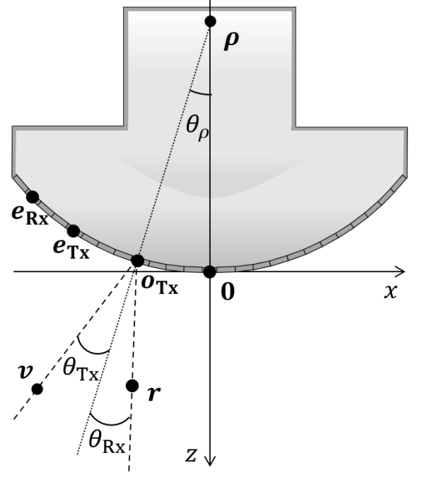
Figure 1: Visualization of imaging setup with the coordinate system origin $\mathbf{0}=\left[0,0,0\right]^{T}$. The figure shows the transmit origin $\mathbf{o_{\text{Tx}}}$, the receive element $\mathbf{e_{\text{Rx}}}$, the transmit element $\mathbf{e_{\text{Tx}}}$, the transmit focus position (virtual source) $\mathbf{v}$ and pixel position $\mathbf{r}$.

2.1 Wave propagation model

The model chosen to estimate and correct sound speed errors assumes that the wave propagation from the active transmit aperture to a pixel and back to the receivers acts as a global sound speed with individual values for individual pixels. The sound speed values in the map are the average of the different straight ray paths between the $N$ active transmit elements, the pixels, and the $M$ receive elements. This spatially distributed average sound speed $c_{\text{avg}}(\mathbf{r})$ is expressed as

$$c_{\text{avg}}(\mathbf{r})=\frac{1}{MN}\sum_{m=1}^{M}\sum_{n=1}^{N}c_{\text{har}}(\mathbf{r},\mathbf{e}_{\text{Tx}}(n))+c_{\text{har}}(\mathbf{r},\mathbf{e}_{\text{Rx}}(m)),$$ (1)

where $c_{\text{har}}(\mathbf{r},\mathbf{e})$ is the one-way harmonic average of the local sound speed from element position $\mathbf{e}$ to pixel position $\mathbf{r}$, given by

$$c_{\text{har}}(\mathbf{r},\mathbf{e})^{-1}=\frac{1}{\|\mathbf{r}-\mathbf{e}\|_{2}}\displaystyle\int\limits_{0}^{\|\mathbf{r}-\mathbf{e}\|_{2}}\frac{dl}{c_{\text{local}}(\mathbf{e}+l(\mathbf{r}-\mathbf{e})/\,\|\mathbf{r}-\mathbf{e}\|_{2})},$$ (2)

where $\|\cdot\|_{2}$ is the Euclidean norm and $l$ is the straight path length integrated over. The assumption neglects refraction and will interpret any hyperbolic delay aberration as an error in sound speed. This can lead to an aberration ambiguity as illustrated in Fig. 2. This simplified model of wave propagation captures a first-order approximation of the propagation in a medium with heterogeneous sound speed. Refraction and phase aberrations are here treated as second-order effects. Accounting for refraction is more complicated as it is sensitive to the accuracy of the estimated local sound speed map [15].

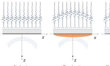
(a) No aberration.

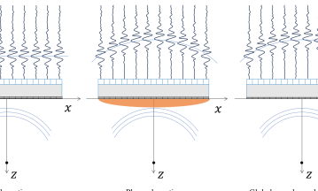
(b) Lens aberration.

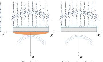
(c) Wrong global sound speed aberration.

Figure 2: Illustration of received signal from a point scatter after focusing. The received signals are similar for (b) and (c) even though (b) is aberrated by a lens and (c) is aberrated by an incorrect global sound speed.

The aberration correction is performed directly by beamforming with the average sound speed map $c_{\text{avg}}$.

Note that the spatial variation of the average sound speed maps is expected to be smooth for longer path lengths due to the cumulative integration in (2).

2.2 Beamforming with average sound speed map

During beamforming we assume the simplified wave propagation model from Section 2.1 and use a spatial weighted REFoCUS [16] implementation given as

$$b(\mathbf{r})=\sum_{m=1}^{M}\sum_{k=1}^{K}\sum_{n=1}^{N}w(\mathbf{r},m,k,n)\,s(k,m,t(\mathbf{r},m,k,n)),$$ (3)

where $s(k,m,t)$ is the analytic channel data signal, and $M$, $K$ and $N$ are the number of active receive elements, transmit events and transmit elements, respectively. The two-way TOF $t$ is expressed as

$$\begin{split}t(\mathbf{r},m,k,n)&=\frac{\|\mathbf{v}(k)-\mathbf{o_{Tx}}(k)\|-\|\mathbf{v}(k)-\mathbf{e_{Tx}}(n,k)\|}{c_{0}}\\ &+\frac{\|\mathbf{r}-\mathbf{e_{Tx}}(n,k)\|}{c_{\text{avg}}(\mathbf{r})}+\frac{\|\mathbf{r}-\mathbf{e_{Rx}}(m)\|}{c_{\text{avg}}(\mathbf{r})},\end{split}$$ (4)

where the first term is the reversed applied transmit delay and uses the assumed sound speed $c_{0}$. The second and third terms are the transmit and receive TOF respectively, and use the average sound speed which is a function of pixel position $\mathbf{r}$.

2.2.1 Pixel-grid compensation

The spatial mapping from time to space in a pixel-based beamformer depends on the speed of sound. This becomes important for the comparison of the focusing quality from pixel to pixel because it can bias the estimation if not taken into account [11, 17]. The bias is mitigated by compensating the scan grid to maintain the geometry assumed on transmission (computed with $c_{0}$). The geometry compensation of the pixel depth is a simple scaling by the sound speed ratio starting at the receive beam origin, given as

$$\|\mathbf{r}-\mathbf{o_{Tx}}\|=\frac{c_{\text{avg}}(\mathbf{r})}{c_{0}}\|\mathbf{r}_{0}-\mathbf{o_{Tx}}\|.$$ (5)

The angle of pixels changes with a change of sound speed according to Snell-Descartes law of refraction as

$$\theta_{\text{Rx}}(\mathbf{r})=\arcsin{\left(\frac{c_{\text{avg}}(\mathbf{r})}{c_{0}}\sin{\left(\theta_{\text{Rx0}}(\mathbf{r})\right)}\right)},$$ (6)

where $\theta_{\text{Rx0}}(\mathbf{r})$ is the angle in the coordinate system computed with the sound speed $c_{0}$ and $\theta_{\text{Rx}}(\mathbf{r})$ computed with $c_{\text{avg}}(\mathbf{r})$. The compensation makes all structures stationary while varying $c_{\text{avg}}(\mathbf{r})$. This is also beneficial because geometric measurements and standardized clinical indices are established with the scan grid obtained with $c_{0}=1540$.

2.3 Average sound speed estimation

The average sound speed can be found by retrospectively focusing the same data set using multiple global sound speeds and choosing a sound speed value for every pixel that optimizes a focusing quality metric [10, 8, 17]. We employ a similar optimization using the coherence factor $C_{R}$ in (7), suggested in [18].

$$C_{R}(\mathbf{r})=\frac{\left|\sum_{m=1}^{M}\hat{b}(\mathbf{r},m)\right|}{\sum_{m=1}^{M}\left|\hat{b}(\mathbf{r},m)\right|},$$ (7)

where $\hat{b}(\mathbf{r},m)$ is the beamsum, that is, the delay-and-summed channel data, summed over $K$ transmit events and $N$ transmit elements, given as

$$\hat{b}(\mathbf{r},m)=\sum_{k=1}^{K}\sum_{n=1}^{N}w(\mathbf{r},m,k,n)\,s(k,m,t(\mathbf{r},m,k,n)).$$ (8)

The numerator in (7) is the coherent sum of the received signals $s$ and the denominator is the incoherent sum.

2.4 Optimal sound speed selection near a strong scatterer

Adaptive coherence-based beamformers are known to effectively suppress side lobes in regions near strong scatterers [19]. Coherence maximization in these regions may choose an incorrect sound speed because incorrect sound speeds will suppress sidelobes less efficiently.

Maximization of coherence in a region adjacent to a strong scatterer is then susceptible to an erroneous speed of sound selection because this will actually lead to a higher sidelobe level here (see illustration in Fig. 3).

Such problems can be mitigated by spatial expanding of the coherence values in each of the coherence images before selecting the maximum across different sound speeds. Spatial expansion can be implemented using an image processing technique called percentile or rank filtering [20]. This filtering operation is performed with a 2D kernel sliding over the image picking a high percentile coherence value within the kernel. The 50th percentile and 100th percentile versions of such a filter are equivalent to a median filter and image dilation, respectively. The 90th percentile is used for the methods in this paper. Figure 3 illustrates how the percentile filter works by practically expanding the main lobe of the Point Spread Function (PSF) of the system, thus ensuring that the maximum coherence value is also selected off-axis from a strong scatterer.

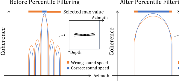
(a) No percentile filter.

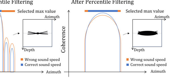
(b) With percentile filter.

Figure 3: Illustration of Point Spread Function (PSF) beamformed with correct and wrong speed of sound. The bar on top in (a) shows that the max value is chosen to be the PSF using correct sound speed in the mainlobe, but incorrect sound speed in the sidelobes. After percentile filtering in (b) the correct sound speed is chosen in the sidelobes as well.

3 Method

The sound speed correction is implemented in the python beamforming library vbeam [21]. The distributed sound speed aberration correction is performed in five steps:

1. Calculate multiple coherence factor images with constant sound speed (1440, 1450,…,$1640\text{\,}\mathrm{m}\text{/}\mathrm{s}$).

2. Threshold, smooth and rank filter the coherence images.

3. Select the sound speed with highest coherence.

4. Median filter and smooth the sounds speed map.

5. Beamform the channel data using the average sound speed map from 4).

The steps are described in more detail below, and the parameter values and kernel sizes for all filters are provided in Tables 2 and  3.

The coherence images in Step 1) are beamformed from harmonic filtered channel data using the expression in (7) and use the TOF calculation in (4) with constant sound speed values $c(\mathbf{r})=c$. The pixel-grid compensation in (5)-(6) is applied for the different coherence images.

In Step 2), we first replace some of the coherence values inside a mask. The mask is the logical union of three pixel regions; pixels where the coherence values are less than 0.2, a depth region in the extreme nearfield and at the scan sector borders (given as a percentage of the scan sector width in Tables 2 and 3). The coherence values inside the mask are replaced by the mean value of the coherence values outside the mask; $C_{R}[P]\leftarrow\overline{C_{R}[\neg P]}$, where $P$ is the logical mask, $\neg$ is the negation operator, and $\overline{\text{overline}}$, indicate the mean value. Secondly, the coherence images are smoothed with a 2D Gaussian window to average measurement noise. A moving average is also applied for each pixel over the sound speed dimension, smoothing the coherence as a function of the sound speed. Finally, a 2D rank filtering, described in Section 2.4, mitigates the influence from off-axis scatterers.

In Step 3) the sound speed with maximum coherence, after the processing in Step 2), is selected for each pixel independently. In Step 4) a 2D median filter is applied to remove outliers from the map. Secondly, the average sound speed map is smoothed with a 2D kernel size that increases linearly with depth. This increase is done because the average sound speed map is expected to be smoother at higher depths.

The aberration correction in Step 5) is performed by beamforming the channel data using the expression in (3) and the TOF calculated using the average sound speed map from Step 3).

Final displayed images were processed and visualized with software running the same image processing libraries as those used on the Voluson Expert 22 scanner. In this way, the change in image quality from the proposed sound speed correction method can be evaluated on the basis of clinically relevant images.

3.1 Validation in controlled settings

The validity of the distributed aberration correction method is tested in silico and in vitro.

3.1.1 In-silico

Three K-wave simulations [22] using a linear scan and focused transmissions are executed in a medium with different local sound speed maps. The simulation assumes $1540\text{\,}\mathrm{m}\text{/}\mathrm{s}$ during transmit focusing and images a speckle scene with point targets. The channel data from the simulations are recorded and average sound speed is estimated with the proposed method. To evaluate the precision of the estimate, the ground-truth average sound speed is calculated from the true local sound speed maps using (1). The assumed sound speed during transmit is $1540\text{\,}\mathrm{m}\text{/}\mathrm{s}$ and 21 sound speed values (1440, 1450, … $1640\text{\,}\mathrm{m}\text{/}\mathrm{s}$) are used in the estimation process. The simulation settings and processing settings are found in Table 1 and Table 2 respectively.

Table 1: K-wave simulation setup.

Parameter	Value	Units
Number of elements	128	-
Array pitch	400	$\mu$m
Pulse	Gaussian 2-cycles	-
Center frequency	4	MHz
Transmit focus depth	30	mm
Grid spacing	100	$\mu$m
Grid dimension	1080$\times$1024	pixels
Medium density	1020	kg/m3

Table 2: Aberration correction settings for the K-wave simulation.

Parameter	Value	Units
Step 2)
Extreme nearfield depth	3	mm
Valid percentage of sector	100	%
2D Gaussian kernel size	6$\times$5	mm$\times$mm
Moving average length	3	-
Percentile kernel size	8$\times$2	mm$\times$mm
Step 4)
Median filter size	4$\times$6	mm$\times$mm
2D kernel size	18 $\times$8	mm$\times$mm
Lateral increase rate	0.3	mm/mm
Axial increase rate	0.3	mm/mm

3.1.2 In vitro

Two sets of channel data are collected from the same CIRS general-purpose phantom, assuming different sound speeds during transmission. The phantom has a sound speed of $1540\text{\,}\mathrm{m}\text{/}\mathrm{s}$. Data were collected using the Voluson Expert 22 scanner and the eM6C curvilinear matrix-array probe from GE HealthCare (GE HealthCare Women’s Health Ultrasound, Zipf, Austria). The Expert 22 system allows for storage of channel data for offline processing. The eM6c use Sub-Aperture technology to limit the number of channels [23]. The two recordings are collected to test the sound speed estimators on the sound speed assumption during transmission. The probe position is stationary for the two recordings. The settings used in the aberration correction process for the in vitro and in vivo images are given in Tab. 3.

Table 3: Aberration correction settings for the eM6C probe.

Parameter	Value	Units
Step 2)
Extreme nearfield depth	10	mm
Valid percentage of sector	80	%
2D Gaussian kernel size	10$\times$5	degrees$\times$mm
Moving average length	3	-
Percentile kernel size	5$\times$3	degrees$\times$mm
Step 4)
Median filter size	10$\times$10	degrees$\times$mm
2D kernel size	20 $\times$10	degrees$\times$mm
Lateral increase rate	0.803	degrees/mm
Axial increase rate	0.6	mm/mm

3.2 Clinical validation of method

A total of 172 Bmode images of clinical standard views for fetal biometry and echocardiography were obtained in week 18-20 and 32, including BiParietal Diameter (BPD), Mean Abdominal Diameter (MAD), Femur Length (FL), Four chamber view (4CV), Pulmonary Valve Diameter (PVD) and Aortic Valve Diameter (AVD). The data were collected with the eM6C probe on the Voluson Expert 22 system at St. Olavs hospital, Trondheim University Hospital, Norway. Endurance training and time restricted eating before and during pregnancy” were invited and provided written informed consent. The project is approved by the Mid-Norway Regional Committee for Medical and Health Research Ethics. The patients provided written informed consent under a data collection agreement approved by the Mid-Norway Regional Committee for Medical and Health Research Ethics. The data were captured using a focused walking aperture transmit sequence assuming $1540\text{\,}\mathrm{m}\text{/}\mathrm{s}$ on transmit. The images are aberration corrected with the proposed method and settings used in this process are similar to the in vitro experiment given in Tab. 3.

3.2.1 Clinical evaluation

One midwife with 8 years of experience and two medical doctors with 15 and 25 years of experience, all from the Fetal Medicine Department at St. Olavs hospital, evaluated the clinical relevance of the sound speed correction. The clinicians were presented with two images, one using $1540\text{\,}\mathrm{m}\text{/}\mathrm{s}$ and one corrected for aberration, and they selected their preferred image. The clinicians also had the option to mark the image quality as similar. The image pairs were randomly shuffled in the evaluation. The clinicians have

3.2.2 Tenengrad sharpness

Tenengrad sharpness is a robust and accurate measure for focusing quality and performs well in digital photography [24, 25]. The Tenengrad measure is the magnitude of the Sobel filtered image. Because the correct speed of sound mostly affects the lateral focusing quality in pulse echo ultrasound, we use the lateral Sobel filter expressed as

$$\mathbf{G}(\mathbf{r})=\begin{bmatrix}1&0&-1\\ 2&0&-2\\ 1&0&-1\end{bmatrix}*\mathbf{A}(\mathbf{r}),$$ (9)

where the image $\mathbf{A}$ is convolved with the matrix to produce the image $\mathbf{G}$. The Tenengrad measure $F$ is calculated by summing the magnitude of the filtered image $\mathbf{G}$ as

$$F=\sum_{\mathbf{r}\in\text{ROI}}|\mathbf{G}(\mathbf{r})|$$ (10)

where the sum of pixels $\mathbf{r}$ is within a Region Of Interest (ROI) consisting of all angles within the transmitted beam sector and a depth axis beginning at $10\text{\,}\mathrm{m}\mathrm{m}$ to avoid measuring contributions from near-field artifacts. The percentage increase of image sharpness between the image corrected for sound speed and the uncorrected image is given as

$$\kappa=100\left(\frac{F_{\text{corrected}}}{F_{\text{uncorrected}}}-1\right).$$ (11)

We expect the sharpness to be correlated with the proposed sound speed correction method. To test this, we calculate the Mean Absolute Deviation (MAD) of the estimated average sound speed map from $1540\text{\,}\mathrm{m}\text{/}\mathrm{s}$ and measure the Pearson Correlation Coefficient (PCC) between the MAD and the Tenengrad image quality increase $\kappa$.

4 Results

4.1 Simulated experiments

Speckle, point targets and different sound speed maps are simulated in K-wave. Fig. 4a shows the Bmode of the medium, beamformed using the true sound speed. Fig. 4 shows the estimated sound speed maps for true constant $1480\text{\,}\mathrm{m}\text{/}\mathrm{s}$ and $1610\text{\,}\mathrm{m}\text{/}\mathrm{s}$ values. Fig. 5 shows the true local, true averaged and the estimated sound speed maps for a layered medium. The true average map in Fig. 5b is calculated from the local map in Fig. 5a using the wave propagation model assumed in (1). The estimated map follows the procedures in Section 3.

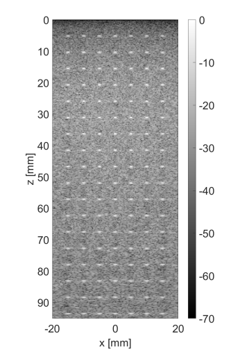
(a) Correctly
focused Bmode of
$1480\text{\,}\mathrm{m}\text{/}\mathrm{s}$ simulation.

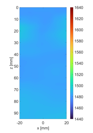
(b) Estimated map
of constant $1480\text{\,}\mathrm{m}\text{/}\mathrm{s}$
map. MAE=$4.78\text{\,}\mathrm{m}\text{/}\mathrm{s}$.

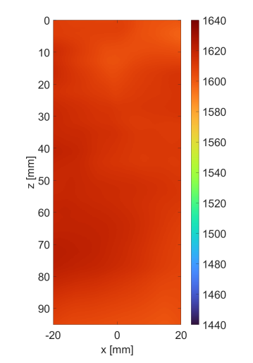
(c) Estimated map
of constant $1610\text{\,}\mathrm{m}\text{/}\mathrm{s}$
map. MAE=$4.74\text{\,}\mathrm{m}\text{/}\mathrm{s}$.

Figure 4: Estimated average sound speed map from in silico speckle phantoms with point targets and constant global sound speeds. The Mean Absolute Error (MAE) from the ground truth is written in the subcaptions.

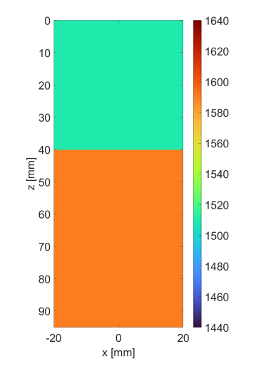
(a) Local map.

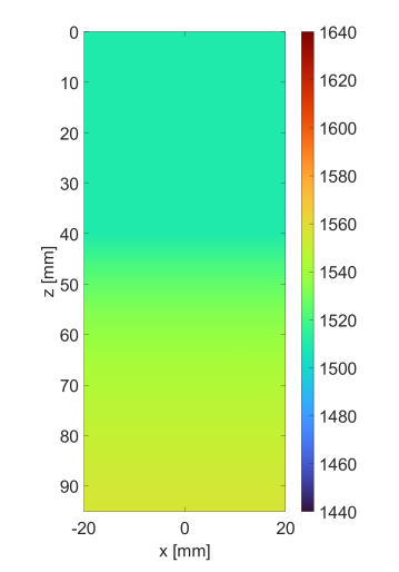
(b) True average.

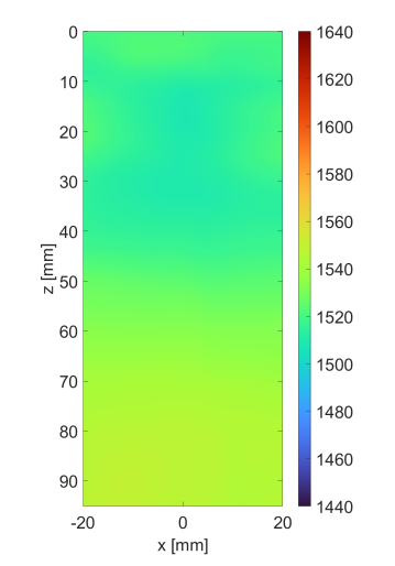
(c) Estimated average. MAE=4.31.

Figure 5: Local, true average and estimated average sound speed map from in silico phantom with speckle, point targets and a layered sound speed map. The Mean Absolute Error (MAE) from the ground truth is found in the subcaption.

4.2 In vitro experiments

The Voluson Expert 22 scanner has the option to set the sound speed to different constant values (OTI parameter). Two channel data sets from the same CIRS phantom are collected assuming $1540\text{\,}\mathrm{m}\text{/}\mathrm{s}$ and $1480\text{\,}\mathrm{m}\text{/}\mathrm{s}$. The effective focus position and the scan grid will change between the two acquisitions as a consequence of changing sound speed [11]. The estimated average sound speed map and Bmode images are shown in Fig. 6.

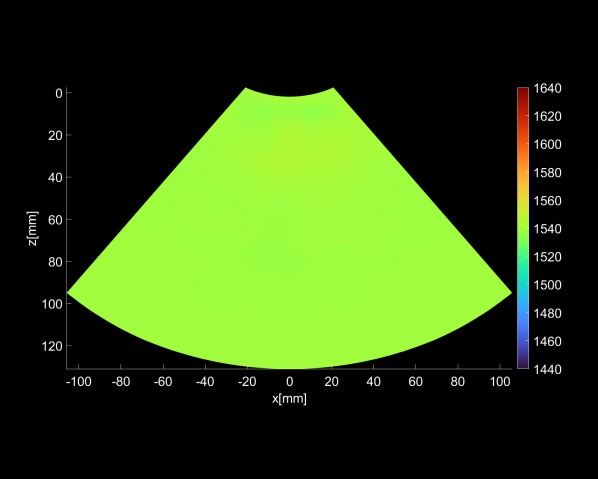
(a) Estimated sound speed map.
assuming $1540\text{\,}\mathrm{m}\text{/}\mathrm{s}$ on transmit.
MAE = $1.05\text{\,}\mathrm{m}\text{/}\mathrm{s}$.

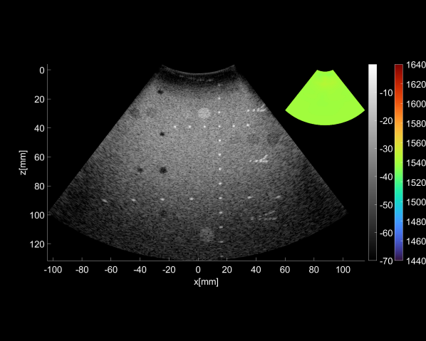
(b) Aberration corrected Bmode
assuming $1540\text{\,}\mathrm{m}\text{/}\mathrm{s}$ on transmit.

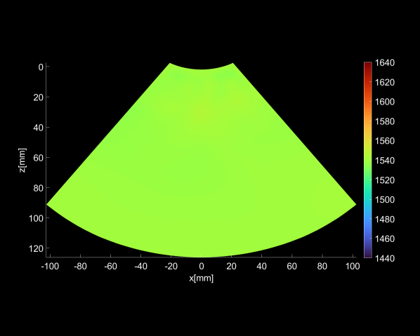
(c) Sound speed map estimated
assuming $1480\text{\,}\mathrm{m}\text{/}\mathrm{s}$ on transmit.
MAE = $1.26\text{\,}\mathrm{m}\text{/}\mathrm{s}$.

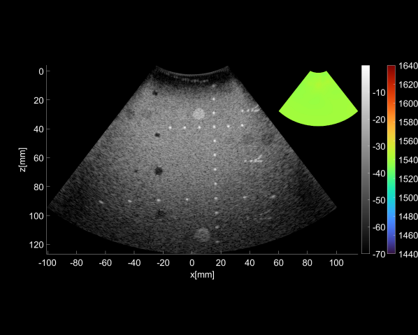
(d) Aberration corrected Bmode
assuming $1480\text{\,}\mathrm{m}\text{/}\mathrm{s}$ on transmit.

Figure 6: Estimated average sound speed maps and Bmode images of two collections of a CIRS $1540\text{\,}\mathrm{m}\text{/}\mathrm{s}$ phantom. The recordings differ in the assumed sound speed during transmission.

4.3 Clinical in vivo validation

All the 172 pairs of corrected and uncorrected clinical fetal Bmode images have been evaluated by three clinicians and image quality improvement has been estimated using the Tenengrad image quality metric $F$ from Section 3.2.2.

The average value of the estimated average sound speed maps provides global values for each image in the dataset. The distribution of the global values over the entire dataset is shown in Fig. 7.

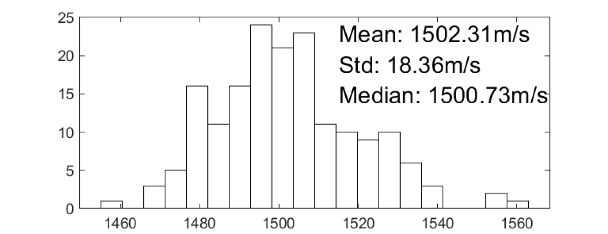
Figure 7: Distribution of estimated global speed of sound values in 172 in vivo fetal images.

Table 4 presents the evaluations of each clinician and shows that the proposed method is preferred or creates a quality similar to the uncorrected image in 72.5% (50.6%+21.9%) of the cases. Box plots of the global average sound speed estimates labeled by the evaluators are shown in Fig. 8.

Table 4: Clinical evaluation of image quality.

	Prefer corrected	Prefer $1540\text{\,}\mathrm{m}\text{/}\mathrm{s}$	Similar quality
Evaluator 1	95	47	30
Evaluator 2	66	29	77
Evaluator 3	100	66	6
Sum	261	142	113
Percentage	50.6%	27.5%	21.9%

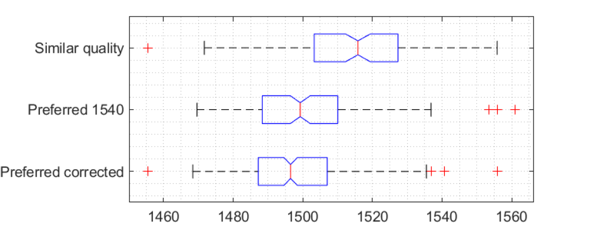
Figure 8: Distribution of the estimated global speed of sound values in the population of images label by the clinical evaluators. The notch indicate 95% confidence of the median. The median of ”similar quality” is statistically different from the others by the Wilcoxon rank sum test.

The percentage increase in image sharpness, $\kappa$, is calculated according to (11). The increase is plotted as a function of the estimated sound speed deviation in Fig. 9. The Pearson Correlation Coefficient (PCC) is measured to be 0.67.

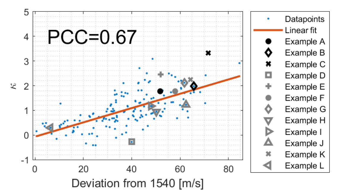
Figure 9: Percentage increase of image quality by correcting for sound speed instead of using $1540\text{\,}\mathrm{m}\text{/}\mathrm{s}$. The quality is measured using the image power after lateral Sobel filtering. Examples A-C are visualized in Figs. 10 -12 and D-L (in gray) are found in supplementary materials.

Table 5: Tabular values and evaluation answers from 12 case examples.

Example	A	B	C	D	E	F	G	H	I	J	K	L
Global speed estimate [$\mathrm{m}\text{/}\mathrm{s}$]	1488	1474	1468	1500	1488	1482	1478	1490	1492	1478	1475	1534
Sharpness increase ($\kappa$)	1.78	1.98	3.33	-0.28	2.46	1.77	2.12	0.95	1.17	1.23	2.25	0.30
Corrected preferred	3	2	3	1	2	3	1	3	3	0	3	0
Uncorrected preferred	0	1	0	1	1	0	2	0	0	3	0	0
Similar quality	0	0	0	1	0	0	0	0	0	0	0	3

Three in vivo Bmode fetal images with and without aberration correction are presented in Figs. 10-12. GIF images of examples A-L (see Fig. 9 and Table 5) alternating between the corrected and uncorrected images are uploaded as supplementary material. The differences in image quality are easier to appreciate in the GIFs than in a side-by-side comparison. The data points for the three examples are colored black in Fig. 9. Table 5 give tabular values for the global sound speed estimate, sharpness increase ($\kappa$) and answers from the clinical evaluations.

Each aberration-corrected Bmode image is gained to have the same 80th percentile pixel intensity value as the 80th percentile value of the corresponding uncorrected image. The Bmode images are plotted in dB relative to the max of the uncorrected image.

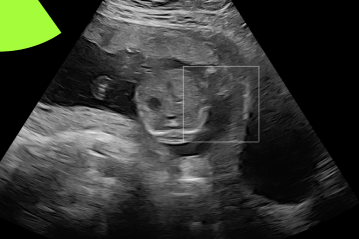
(a) Uncorrected Bmode.

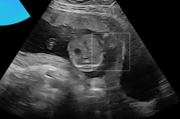
(b) Aberration corrected Bmode.

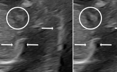
(c) Uncorrected Bmode.

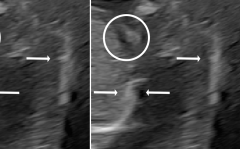
(d) Corrected Bmode.

Figure 10: Example A. In vivo fetal Bmode image using constant $1540\text{\,}\mathrm{m}\text{/}\mathrm{s}$ and the estimated average sound speed map. The average sound speed map is shown in the top right corner and the rightmost colorbar indicates the sound speed values. Alternating GIFs are found in the supplementary material.

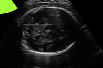
(a) Uncorrected Bmode.

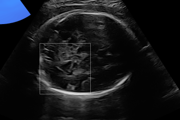
(b) Aberration corrected Bmode.

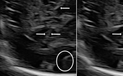
(c) Uncorrected Bmode.

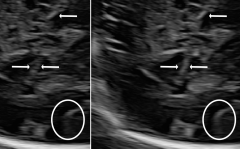
(d) Corrected Bmode.

Figure 11: Example B. In vivo fetal Bmode image using constant $1540\text{\,}\mathrm{m}\text{/}\mathrm{s}$ and the estimated average sound speed map. The average sound speed map is shown in the top right corner and the rightmost colorbar indicates the sound speed values. Alternating GIFs are found in the supplementary material.

(a) Uncorrected Bmode.

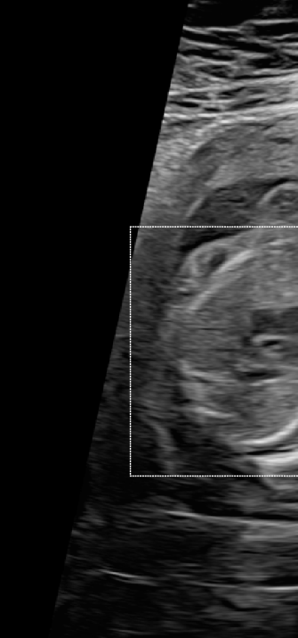
(b) Aberration corrected Bmode.

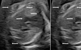
(c) Uncorrected Bmode.

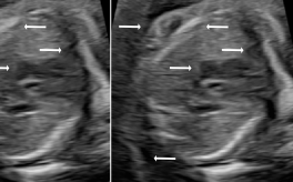
(d) Corrected Bmode.

Figure 12: Example C. In vivo fetal Bmode and coherence images using constant $1540\text{\,}\mathrm{m}\text{/}\mathrm{s}$ and the estimated average sound speed map. The average sound speed map is shown in the top right corner and the rightmost colorbar indicates the sound speed values. Alternating GIFs are found in the supplementary material.

5 Discussion

The estimated average sound speed maps for the simulated phantoms with known local maps show similarity to the true average map in the constant and layered cases. The results are similar to experiments without point targets published by Ali et al. in [10].

The sound speed estimation of the two CIRS phantom recordings appears to be similar, indicating that the estimator is independent of the assumed sound speed during transmission. This is important for in vivo estimation because a potentially wrong sound speed is assumed when calculating aperture delays for a focused transmission. The phantom is manufactured to have a constant $1540\text{\,}\mathrm{m}\text{/}\mathrm{s}$, and deviations in estimated sound speed can be a consequence of phantom wear or inaccuracies with the proposed method.

The quantitative measurement of image sharpness in Fig. 9 shows a general increase in sharpness when correcting for a deviation in sound speed. The measured Pearson Correlation Coefficient (PCC) of 0.67 signifies a clear trend.

The distribution of the estimated sound speed values in Fig. 7 shows about $40\text{\,}\mathrm{m}\text{/}\mathrm{s}$ lower mean value than the conventional sound speed of $1540\text{\,}\mathrm{m}\text{/}\mathrm{s}$. A similar finding was observed in a clinical research paper by Chauveau et al., where images assuming $1480\text{\,}\mathrm{m}\text{/}\mathrm{s}$ were graded with higher quality than the images focused assuming $1540\text{\,}\mathrm{m}\text{/}\mathrm{s}$ [4]. Based on this, a lower default sound speed value could be considered for obstetric ultrasound.

The distribution labeled as ”similar quality” in Fig. 8 shows a mean estimated sound speed value closer to $1540\text{\,}\mathrm{m}\text{/}\mathrm{s}$ than the other distributions. This is expected because images with an estimated sound speed close to $1540\text{\,}\mathrm{m}\text{/}\mathrm{s}$ will have a similar appearance to the uncorrected $1540\text{\,}\mathrm{m}\text{/}\mathrm{s}$ image. Example L, found in the supplementary material, has an estimated sound speed of 1534 and is evaluated by all evaluators as ”similar quality”.

The in vivo examples A-C, in Figs. 10-12 respectively, show different nuances of how sound speed aberration correction improves focusing quality. A noticeable improvement in Fig. 10 is the improved contrast and clarity of borders. The sound speed correction seems to remove the double structure indicated by the arrows in Figs. 10c-10d. The skull border and the brain structures in Fig. 11 are also better defined and clearer after aberration correction. Example C in Fig. 12 is the image with the highest increase in Tenengrad $\kappa$, seen from Fig. 9 and Table 5. The improvement in image quality is evident around the boundary of the fetus body and the correction sharpens the structures indicated by the arrows. The improved contrast between the layers in the shallow tissue layers is also noticeable.

Some of the measured sharpness values decrease after the correction, as seen in Fig. 9. Example D, found in the supplementary material, is one of them. The sound speed correction of Example D seems to make structures more continuous, which results in less high frequent lateral variations in the image and a lower Tenengrad value. This is a weakness of the Tenengrad sharpness measurement. The clinical evaluations answered differently for this image, as seen in Table 5.

Example J, found in the supplementary material, shows images of a fetal head for which the three evaluators preferred the $1540\text{\,}\mathrm{m}\text{/}\mathrm{s}$ image. The sound speed correction seems to sharpen the skull and tissue outside the head, but seems to defocus the structures on the left-hand side of center inside the head. A potential fix for this case is to use a smaller kernel size for smoothing the sound speed map, enabling more rapid spatial variations in average sound speed. Example G shows similar mixed corrections, and the corrected image was preferred by one clinician and the uncorrected preferred by two.

It is interesting to note the difference in the classification done by the evaluators. It is apparent that the evaluators have different opinions of what makes two images of ”similar quality”, as one evaluator classified 77 images as such and another only 6.

Further work will investigate what causes clinical evaluators to prefer the $1540\text{\,}\mathrm{m}\text{/}\mathrm{s}$ over the estimated sound speed in 27.5% of the cases. One hypothesis for this is that the proposed method may choose sound speeds that focuses the images well in most part of the image, but not particularly at some clinical relevant structure, as seen in Example J and G. 2D matrix arrays can dynamically focus in the elevation direction, and it is expected that focusing with the true sound speed will obtain a narrower main lobe and lower sidelobes in elevation. This can explain some of the structure changes seen between corrected and uncorrected images and may be a reason for clinicians to prefer the uncorrected image.

6 Conclusion

This work shows that retrospective two-way aberration correction, based on coherence maximization of the distributed sound speed, is feasible and enhances image quality in obstetric imaging. The increase in image quality is quantified for 172 images with a metric from digital photography, and the results show that sharpness increases when sound speed correction is performed. The aberration correction improves resolution and contrast, yielding clearer structures, better-defined borders, and sharper edges. The clinical evaluation shows that the proposed method is preferred or creates an image quality similar to $1540\text{\,}\mathrm{m}\text{/}\mathrm{s}$ images for 72.5% of the 172 cases. The simulation and phantom studies show that the method is unbiased against the assumed sound speed on transmission and that the proposed aberration correction technique is equivalent to focusing using the ground truth distributed average sound speed map. For the data collected in this study, a sound speed of around $1500\text{\,}\mathrm{m}\text{/}\mathrm{s}$ is found to be a better choice for fetal imaging.

References

- [1] Rehman Ali et al. “Aberration correction in diagnostic ultrasound: A review of the prior field and current directions” In Zeitschrift für Medizinische Physik, 2023 DOI: 10.1016/j.zemedi.2023.01.003
- [2] Haim Azhari “Appendix A: Typical Acoustic Properties of Tissues” In Basics of Biomedical Ultrasound for Engineers John Wiley & Sons, Ltd, 2010, pp. 313–314 URL: https://onlinelibrary.wiley.com/doi/abs/10.1002/9780470561478.app1
- [3] Jodi S. Dashe, Donald D. McIntire and Diane M. Twickler “Maternal obesity limits the ultrasound evaluation of fetal anatomy” In Journal of Ultrasound in Medicine: Official Journal of the American Institute of Ultrasound in Medicine 28.8, 2009, pp. 1025–1030 DOI: 10.7863/jum.2009.28.8.1025
- [4] B. Chauveau et al. “Improving image quality of mid-trimester fetal sonography in obese women: role of ultrasound propagation velocity” In Ultrasound in Obstetrics & Gynecology 52.6, 2018, pp. 769–775 DOI: 10.1002/uog.19015
- [5] Patrick Stähli, Martin Frenz and Michael Jaeger “Bayesian Approach for a Robust Speed-of-Sound Reconstruction Using Pulse-Echo Ultrasound” Conference Name: IEEE Transactions on Medical Imaging In IEEE Transactions on Medical Imaging 40.2, 2021, pp. 457–467 DOI: 10.1109/TMI.2020.3029286
- [6] Samuel Beuret et al. “Windowed Radon Transform for Robust Speed-of-Sound Imaging With Pulse-Echo Ultrasound” Conference Name: IEEE Transactions on Medical Imaging In IEEE Transactions on Medical Imaging 43.4, 2024, pp. 1579–1593 DOI: 10.1109/TMI.2023.3343918
- [7] William Lambert et al. “Ultrasound Matrix Imaging—Part II: The Distortion Matrix for Aberration Correction Over Multiple Isoplanatic Patches” Conference Name: IEEE Transactions on Medical Imaging In IEEE Transactions on Medical Imaging 41.12, 2022, pp. 3921–3938 DOI: 10.1109/TMI.2022.3199483
- [8] Rehman Ali et al. “Distributed Aberration Correction Techniques Based on Tomographic Sound Speed Estimates” Conference Name: IEEE Transactions on Ultrasonics, Ferroelectrics, and Frequency Control In IEEE Transactions on Ultrasonics, Ferroelectrics, and Frequency Control 69.5, 2022, pp. 1714–1726 DOI: 10.1109/TUFFC.2022.3162836
- [9] David Napolitano et al. “Sound speed correction in ultrasound imaging” In Ultrasonics 44, 2006, pp. e43–e46 DOI: 10.1016/j.ultras.2006.06.061
- [10] Rehman Ali et al. “Local Sound Speed Estimation for Pulse-Echo Ultrasound in Layered Media” In IEEE Transactions on Ultrasonics, Ferroelectrics, and Frequency Control 69.2, 2022, pp. 500–511 DOI: 10.1109/TUFFC.2021.3124479
- [11] Anders Emil Vrålstad, Ole Marius Hoel Rindal, Tore Grüner Bjåstad and Svein-Erik Måsøy “Sound Speed and Virtual Source Correction in Synthetic Transmit Focusing” Conference Name: IEEE Open Journal of Ultrasonics, Ferroelectrics, and Frequency Control In IEEE Open Journal of Ultrasonics, Ferroelectrics, and Frequency Control 4, 2024, pp. 52–62 DOI: 10.1109/OJUFFC.2024.3411578
- [12] G.E. Trahey and P.D. Freiburger “An evaluation of transducer design and algorithm performance for two dimensional phase aberration correction” In IEEE 1991 Ultrasonics Symposium,, 1991, pp. 1181–1187 vol.2 DOI: 10.1109/ULTSYM.1991.234302
- [13] Dong-Lai Liu and R.C. Waag “A comparison of ultrasonic wavefront distortion and compensation in one-dimensional and two-dimensional apertures” Conference Name: IEEE Transactions on Ultrasonics, Ferroelectrics, and Frequency Control In IEEE Transactions on Ultrasonics, Ferroelectrics, and Frequency Control 42.4, 1995, pp. 726–733 DOI: 10.1109/58.393115
- [14] Nick Bottenus “Recovery of the Complete Data Set From Focused Transmit Beams” Conference Name: IEEE Transactions on Ultrasonics, Ferroelectrics, and Frequency Control In IEEE Transactions on Ultrasonics, Ferroelectrics, and Frequency Control 65.1, 2018, pp. 30–38 DOI: 10.1109/TUFFC.2017.2773495
- [15] Thurston Brevett, Sergio Sanabria and Jeremy J. Dahl “A Comparison of Global and Local Sound Speed Estimation for Aberration Correction in Abdominal Models” ISSN: 1948-5727 In 2023 IEEE International Ultrasonics Symposium (IUS), 2023, pp. 1–4 DOI: 10.1109/IUS51837.2023.10307733
- [16] Anders Emil Vrålstad, Magnus Dalen Kvalevåg, Ole Marius Hoel Rindal and Svein-Erik Måsøy “Universal REFoCUS beamforming with spatial weighting” Conference Name: IEEE Open Journal of Ultrasonics, Ferroelectrics, and Frequency Control In IEEE Open Journal of Ultrasonics, Ferroelectrics, and Frequency Control, 2024, pp. 1–1 DOI: 10.1109/OJUFFC.2024.3398595
- [17] Rifat Ahmed and Gregg E. Trahey “Spatial Ambiguity Correction in Coherence-Based Average Sound Speed Estimation” Conference Name: IEEE Transactions on Ultrasonics, Ferroelectrics, and Frequency Control In IEEE Transactions on Ultrasonics, Ferroelectrics, and Frequency Control 71.10, 2024, pp. 1244–1254 DOI: 10.1109/TUFFC.2024.3440832
- [18] Kenneth Wayne Rigby “Method and apparatus for coherence filtering of ultrasound images”, 1999 URL: https://patents.google.com/patent/US5910115A/en
- [19] Ole Marius Hoel Rindal, Alfonso Rodriguez-Molares and Andreas Austeng “The Dark Region Artifact in Adaptive Ultrasound Beamforming” In IEEE International Ultrasonics Symposium, IUS, 2017, pp. 1–4 DOI: 10.1109/ULTSYM.2017.8092255
- [20] RM Hodgson et al. “Properties, implementations and applications of rank filters” In Image and Vision Computing 3.1, 1985, pp. 3–14 DOI: 10.1016/0262-8856(85)90037-X
- [21] Magnus Dalen Kvalevåg et al. “vbeam: a Fast and Differentiable Beamformer for Optimizing Ultrasound Imaging” In 2023 IEEE International Ultrasonics Symposium (IUS), 2023
- [22] Bradley E. Treeby and Benjamin T. Cox “k-Wave: MATLAB toolbox for the simulation and reconstruction of photoacoustic wave fields” Publisher: SPIE In Journal of Biomedical Optics 15.2, 2010, pp. 021314 DOI: 10.1117/1.3360308
- [23] Geir Ultveit Haugen, Kjell Kristoffersen and Douglas Glenn Wildes “Ultrasound probe sub-aperture processing”, 2005 URL: https://www.freepatentsonline.com/20050113699.html
- [24] F.. Groen, I.. Young and G. Ligthart “A comparison of different focus functions for use in autofocus algorithms” In Cytometry 6.2, 1985, pp. 81–91 DOI: 10.1002/cyto.990060202
- [25] Hashim Mir, Peter Xu and Peter van Beek “An extensive empirical evaluation of focus measures for digital photography” In Digital Photography X 9023 SPIE, 2014, pp. 167–177 DOI: 10.1117/12.2042350
Acknowledgment
Anders Emil Vrålstad would like to thank Magnus Dalen Kvalevåg for support with the implementation in vbeam. He also thanks Vibeke Skoura-Torsvik and Kjell Å. Salvesen for participating in the clinical evaluation.