Last Update: December 5, 2024

Transformers are Deep Optimizers: Provable In-Context Learning for Deep Model Training

Weimin Wu†‡∗111wwm@u.northwestern.edu Maojiang Su♭∗222sumaojiang@mail.ustc.edu.cn Jerry Yao-Chieh Hu†‡∗333jhu@u.northwestern.edu Zhao Song444magic.linuxkde@gmail.com Han Liu†‡§555hanliu@northwestern.edu

**footnotetext: These authors contributed equally to this work.
${}^{\dagger}\;$Center for Foundation Models and Generative AI, Northwestern University, Evanston, IL 60208, USA
${}^{\ddagger}\;$Department of Computer Science, Northwestern University, Evanston, IL 60208, USA
${}^{\flat}\;$Department of Information and Computing Science, USTC, Hefei, Anhui 230026, China
${}^{\natural}\;$Simons Institute for the Theory of Computing, UC Berkeley, Berkeley, CA 94720, USA
${}^{\S}\;$Department of Statistics and Data Science, Northwestern University, Evanston, IL 60208, USA

We investigate the transformer’s capability for in-context learning (ICL) to simulate the training process of deep models. Our key contribution is providing a positive example of using a transformer to train a deep neural network by gradient descent in an implicit fashion via ICL. Specifically, we provide an explicit construction of a $(2N+4)L$-layer transformer capable of simulating $L$ gradient descent steps of an $N$-layer ReLU network through ICL. We also give the theoretical guarantees for the approximation within any given error and the convergence of the ICL gradient descent. Additionally, we extend our analysis to the more practical setting using $\mathop{\rm{Softmax}}$-based transformers. We validate our findings on synthetic datasets for 3-layer, 4-layer, and 6-layer neural networks. The results show that ICL performance matches that of direct training.

1 Introduction

We study transformers’ ability to simulate the training process of deep models. This analysis is not only practical but also timely. On one hand, transformers and deep models (Brown, 2020; Radford et al., 2019) are so powerful, popular and form a new machine learning paradigm — foundation models. These large-scale machine learning models, trained on vast data, provide a general-purpose foundation for various tasks with minimal supervision (Team et al., 2023; Touvron et al., 2023; Zhang et al., 2022). On the other hand, the high cost of pretraining these models often makes them prohibitive outside certain industrial labs (Jiang et al., 2024; Bi et al., 2024; Achiam et al., 2023). In this work, we aim to push forward this “one-for-all” modeling philosophy of foundation model paradigm (Bommasani et al., 2021) by considering the following research problem:

Question 1.

Is it possible to train one deep model with the ICL of another foundation model?

The implication of Question 1 is profound: if true, one foundation model could lead to many others without resource-intensive pertaining, making foundation models more accessible to general users. In this work, we provide an affirmative example for Question 1. Specifically, we show that transformer models are capable of simulating the training of a deep ReLU-based feed-forward neural network with provable guarantees through In-Context Learning (ICL).

In ICL, the models learn to solve new tasks during inference by using task-specific examples provided as part of the input prompt, rather than through parameter updates (Wei et al., 2024; Shi et al., 2024; Xu et al., 2024; Wei et al., 2023; Bubeck et al., 2023; Achiam et al., 2023; Bai et al., 2023; Min et al., 2022; Garg et al., 2022; Brown, 2020). Unlike standard supervised learning, ICL enables models to adapt to new tasks during inference using only the provided examples. In this work, the new task of our interest is algorithmic approximation via ICL (Wang et al., 2024; Chen et al., 2024a; Bai et al., 2023; Zhang et al., 2023). Specifically, we aim to use the transformer’s ICL capability to replace/simulate the standard supervised training algorithms for $N$-layer networks. To be concrete, we formalize the learning problem of how transformers learn (i) a given function and (ii) a machine learning algorithm (e.g., gradient descent) via ICL, following (Bai et al., 2023).

(i) ICL for Function $f$. Let $f:\mathbb{R}^{d}\rightarrow\mathbb{R}$ be the function of our interest. Suppose we have a dataset $\mathcal{D}_{n}\coloneqq\left\{(x_{i},y_{i})\right\}_{i\in[n]}$, where $\left\{x_{i}\right\}_{i\in[n]}\subseteq\mathbb{R}^{d}$ and $\left\{y_{i}\right\}_{i\in[n]}\subseteq\mathbb{R}$ are the input and output of $f$, respectively. Let $x_{n+1}$ be the test input. The goal of ICL is to use a transformer, denoted by $\mathcal{T}$, to predict $y_{n+1}$ based on the test input and the in-context dataset autoregresively: $\widehat{y}_{n+1}\sim\mathcal{T}(\mathcal{D}_{n},x_{n+1})$. The goal is for the prediction $\widehat{y}_{n+1}$ to be close to $y_{n+1}=f(x)$.

(ii) ICL for Gradient Descent of a Parametrized Model $f(w,\cdot)$. Bai et al. (2023) generalize (i) to include algorithmic approximations of Gradient Descent (GD) training algorithms and explore how transformers simulate gradient descent during inference without parameter updates. They term the simulated GD algorithm “In-Context Gradient Descent (ICGD).” In essence, ICGD enables transformers to approximate gradient descent on a loss function $L_{n}(w)$ for a parameterized model $f(w,\cdot)$ based on a dataset $\mathcal{D}_{n}$. Traditional gradient descent updates $w$ iteratively as $w_{t+1}=w_{t}-\eta\nabla L_{n}(w_{t})$. In contrast, ICGD uses a transformer $\mathcal{T}$ to simulate these updates within a forward pass. Given example data $\mathcal{D}_{n}$ and test input $x_{n+1}$, the transformer performs gradient steps in an implicit fashion by inferring parameter updates through its internal representations, using input context without explicit weight changes. Please see Section 2 for explicit formulation.

In this work, we investigate the case where $f(w,\cdot)$ is a deep feed-forward neural network. We defer the detailed problem setting to Section 2. In comparison to standard ICGD (Bai et al., 2023), ICGD for deep feed-forward networks is not trivial. This is due to two technical challenges:

  • (C1)

    Analytical feasibility of gradient computation for these thick networks.

  • (C2)

    Explicit construction capable of approximating ICGD for such layers and their gradients.

A work similar to ours is (Wang et al., 2024). It demonstrates that the transformer implements multiple steps of ICGD on deep neural networks. However, it requires more layers in the transformer model and fails to consider the $\mathop{\rm{Softmax}}$-transformer. We provide a more detailed comparison in Section B.1. To this end, we present the first explicit expression for gradient computation of $N$-layer feed-forward network (Lemma 1). Importantly, its term-by-term tractability provides key insights for the detailed construction of a specific transformer to train this network via ICGD (Theorem 1).

Contributions. We offer a positive early investigation of Question 1. Our contributions are threefold:

  • Approximation by ReLU-Transformer. For simplicity, we begin with the ReLU-based transformer. For a broad class of smooth empirical risks, we construct a $(2N+4)L$-layer transformer to approximate $L$ steps of in-context gradient descent on the $N$-layer feed-forward networks with the same input and output dimensions (Theorem 1). We then extend this to accommodate varying dimensions (Theorem 5). We also provide the theoretical guarantees for the approximation within any given error (Corollary 1.1) and the convergence of the ICL gradient descent (Lemma 14).

  • Approximation by Softmax-Transformer. We extend our analysis to the $\mathop{\rm{Softmax}}$-transformer to better reflect realistic applications. The key technique is to ensure a qualified approximation error at each point to achieve universal approximation capabilities of the $\mathop{\rm{Softmax}}$-based Transformer (Lemma 16). We give a construction of a $4L$-layer $\mathop{\rm{Softmax}}$ transformer to approximate $L$ steps of gradient descent, and guarantee the approximation and the convergence (Theorem 6).

  • Experimental Validation. We validate our theory with ReLU- and $\mathop{\rm{Softmax}}$-transformers, specifically, ICGD for the $N$-layer networks (Theorem 1, Theorem 5, and Theorem 6). We assess the ICL capabilities of transformers by training 3-, 4-, and 6-layer networks in Appendix G. The numerical results show that the performance of ICL matches that of training $N$-layer networks.

Organization. We show our main results in Theorem 1 and the informal version in Appendix A. Section 2 presents preliminaries. Section 3 presents the problem setup and ICL approximation to GD steps of $N$-layer feed-forward network based on ReLU-transformer. The appendix includes the related works (Section B.1), the detailed proofs of the main text (Appendix D), ICL approximation to GD steps of $N$-layer network based on $\mathop{\rm{Softmax}}$-transformer (Appendix F), the experimental results (Appendix G), and the application to diffusion models (Appendix H).

Notations. We use lower case letters to denote vectors and upper case letters to denote matrices. The index set $\{1,...,I\}$ is denoted by $[I]$, where $I\in\mathbb{N}^{+}$. For any matrices $A\in\mathbb{R}^{n\times n}$, let $\ell_{p}$ norm of $A$ be induced by vector $\ell_{p}$-norm, defined as $\|A\|_{p}:=\sup\{\|Ax\|_{p}:x\in\mathbb{R}^{n}\leavevmode\nobreak\ {\rm with}\leavevmode\nobreak\ \|x\|_{p}=1\}$. For any function $f$ and distribution $P$, we denote $L^{2}(P)$ norm of $f$ as $\norm{f}_{L^{2}(P)}=\mathbb{E}_{P}^{1/2}[||f||_{2}^{2}]$. We use $A[i,j]$ to denote the element in $i$-th row and $j$-th column of matrix $A$. For any matrices $A\in\mathbb{R}^{m\times n}$ and $B\in\mathbb{R}^{m\times n}$, let $\odot$ denotes the Hadamard product: $(A\odot B)[i,j]:=A[i,j]\cdot B[i,j]$. For any matrices $A\in\mathbb{R}^{m\times n}$ and $B\in\mathbb{R}^{p\times q}$, let $\otimes$ denote the Kronecker product:

$\displaystyle A\otimes B:=\begin{bmatrix}&A[1,1]B&\cdots&A[1,n]B\\ &\vdots&\ddots&\vdots\\ &A[m,1]B&\cdots&A[m,n]B\end{bmatrix}.$

2 Preliminaries: In-Context Learning and In-Context Gradient Descent

We present the ideas we built upon: In-Context Gradient Descent (ICGD).

(i) ICL for Function $f$. Let $f:\mathbb{R}^{d}\rightarrow\mathbb{R}$ be the function of our interest. Suppose we have a dataset $\mathcal{D}_{n}\coloneqq\left\{(x_{i},y_{i})\right\}_{i\in[n]}$, where $\left\{x_{i}\right\}_{i\in[n]}\subseteq\mathbb{R}^{d}$ and $\left\{y_{i}\right\}_{i\in[n]}\subseteq\mathbb{R}$ are the input and output of $f$, respectively. Let $x_{n+1}$ be the test input. The goal of ICL is to use a transformer, denoted by $\mathcal{T}$, to predict $y_{n+1}$ based on the test input and the in-context dataset autoregressive: $\widehat{y}_{n+1}\sim\mathcal{T}(\mathcal{D}_{n},x_{n+1})$. For convenience in our analysis, we adopt the ICL notation from (Bai et al., 2023). Specifically, we shorthand $(\mathcal{D}_{n},x_{n+1})$ into an input sequence (i.e., prompt) of length $n+1$ and represent it as a compact matrix $H\in\mathbb{R}^{D\times(n+1)}:=[h_{1},\ldots,h_{n+1}]$ in the form:

$\displaystyle H\coloneqq\begin{bmatrix}x_{1}&x_{2}&\cdots&x_{n}&x_{n+1}\\ y_{1}&y_{2}&\cdots&y_{n}&0\\ q_{1}&q_{2}&\cdots&q_{n}&q_{n+1}\end{bmatrix}\in\mathbb{R}^{D\times(n+1)},\quad q_{i}\coloneqq\begin{bmatrix}0_{D-(d+3)}\\ 1\\ t_{i}\end{bmatrix}\in\mathbb{R}^{D-(d+1)}.$ (2.1)

Here, we choose $D\coloneqq\dim{x_{i}}+\dim{y_{i}}+\dim{q_{i}}=\Theta(d)$. We use $q_{i}$ to fill in the remain $D-(d+1)$ entries in addition to $x_{i}\in\mathbb{R}^{d}$ and $y_{i}\in\mathbb{R}$. The last entry $t_{i}\coloneqq\mathds{1}(i<n+1)$ of $q_{i}$ is the position indicator to distinguish the $n$ in-context examples and the test data. The problem of “ICL for $f$ is to show the existence of a transformer $\mathcal{T}$ that, when given $H$, outputs $\mathcal{T}(H)\in\mathbb{R}^{D\times(n+1)}$ of the same shape, and the “$(d+1,n+1)$ entry of $\mathcal{T}(H)$” provides the prediction $\widehat{y}_{n+1}$. The goal is for the prediction $\widehat{y}_{n+1}$ to be close to $y_{n+1}=f(x)$ measured by some proper loss.

(ii) ICL for Gradient Descent of a Parametrized Model $f(w,\cdot)$. In this work, we aim to use ICL to replace/simulate the standard supervised training procedure for $N$-layer neural networks. To achieve this, we introduce the concept of In-Context Gradient Descent (ICGD) for a parameterized model.

Consider a machine learning model $f(w,\cdot):\mathbb{R}^{D_{w}}\times\mathbb{R}^{d}\rightarrow\mathbb{R}^{d}$, parametrized by $w\in\mathbb{R}^{D_{w}}$. Given a dataset $\mathcal{D}_{n}\coloneqq\left\{(x_{i},y_{i})\right\}_{i\in[n]}\overset{\text{iid}}{\sim}\mathbb{P}$, a typical learning task is to find parameters $w^{\star}$ such that $f(w^{\star},\cdot)$ becomes closest to the true data distribution $\mathbb{P}$. Then, for any test input $x_{n+1}$, we predict: $\widehat{y}_{n+1}=f(w^{\star},x_{n+1})$. To find $w^{\star}$, Bai et al. (2023) configure a transformer to implement gradient descent on $f(w,\cdot)$ through ICL, simulating optimization algorithms during inference without explicit parameter updates. We formalize this In-Context Gradient Descent (ICGD) problem: using a pretrained model to simulate gradient descent on $f(w,\cdot)$ w.r.t. the provided context $(\mathcal{D}_{n},x_{n+1})$.

Problem 1 (In-Context Gradient Descent (ICGD) on Model $f(w,\cdot)$ (Bai et al., 2023)).

Let $\epsilon>0$ and $L\geq 1$. Consider a machine learning model $f(w,x):\mathbb{R}^{D_{w}}\times\mathbb{R}^{d}\rightarrow\mathbb{R}^{d}$ parameterized by $w\in\mathbb{R}^{D_{w}}$. Given a dataset $\mathcal{D}_{n}\coloneqq\left\{(x_{i},y_{i})\right\}_{i\in[n]}\overset{\text{iid}}{\sim}\mathbb{P}$ with $(x_{i},y_{i})\in\mathbb{R}^{d}\times\mathbb{R}^{d}$, define the empirical risk function:

$\displaystyle\mathcal{L}_{n}(w)\coloneqq\frac{1}{2n}\sum_{i=1}^{n}\ell(f(w,x_{i}),y_{i}),\quad\text{where $\ell:\mathbb{R}^{d}\times\mathbb{R}^{d}\rightarrow\mathbb{R}$ is a loss function.}$ (2.2)

Let $\mathcal{W}\subseteq\mathbb{R}^{D_{w}}$ be a closed domain, and ${\rm Proj}_{\mathcal{W}}$ denote the projection onto $\mathcal{W}$. The problem of “ICGD on model $f(w,\cdot)$” is to find a transformer $\mathcal{T}$ with $L$ blocks, each approximating one step of gradient descent using $T$ layers. For any input $H^{(0)}\in\mathbb{R}^{D\times(n+1)}$ in the form of (2.1), the transformer $\mathcal{T}(H^{(0)})$ approximates $L$ steps of gradient descent. Specifically, for $l\in[L]$ and $i\in[n+1]$, the output at layer $Tl$ is: hi(Tl)=[xi;yi;\macc@depthΔ\frozen@everymath\macc@group\macc@set@skewchar\macc@nested@a111w(l);𝟎;1;ti]superscriptsubscript𝑖𝑇𝑙subscript𝑥𝑖subscript𝑦𝑖\macc@depthΔ\frozen@everymath\macc@group\macc@set@skewchar\macc@nested@a111superscript𝑤𝑙01subscript𝑡𝑖h_{i}^{(Tl)}=[x_{i};y_{i};{\macc@depth\char 1\relax\frozen@everymath{\macc@group}\macc@set@skewchar\macc@nested@a 111{w}}^{(l)};\mathbf{0};1;t_{i}], where, with \macc@depthΔ\frozen@everymath\macc@group\macc@set@skewchar\macc@nested@a111w(0)=𝟎\macc@depthΔ\frozen@everymath\macc@group\macc@set@skewchar\macc@nested@a111superscript𝑤00{\macc@depth\char 1\relax\frozen@everymath{\macc@group}\macc@set@skewchar\macc@nested@a 111{w}}^{(0)}=\mathbf{0},

\macc@depthΔ\frozen@everymath\macc@group\macc@set@skewchar\macc@nested@a111w(l)=Proj𝒲(\macc@depthΔ\frozen@everymath\macc@group\macc@set@skewchar\macc@nested@a111w(l1)η(n(\macc@depthΔ\frozen@everymath\macc@group\macc@set@skewchar\macc@nested@a111w(l1))+ϵ(l1))) is updated recursively,\macc@depthΔ\frozen@everymath\macc@group\macc@set@skewchar\macc@nested@a111superscript𝑤𝑙subscriptProj𝒲\macc@depthΔ\frozen@everymath\macc@group\macc@set@skewchar\macc@nested@a111superscript𝑤𝑙1𝜂subscript𝑛\macc@depthΔ\frozen@everymath\macc@group\macc@set@skewchar\macc@nested@a111superscript𝑤𝑙1superscriptitalic-ϵ𝑙1 is updated recursively,\displaystyle{\macc@depth\char 1\relax\frozen@everymath{\macc@group}\macc@set@skewchar\macc@nested@a 111{w}}^{(l)}={\rm Proj}_{\mathcal{W}}\left({\macc@depth\char 1\relax\frozen@everymath{\macc@group}\macc@set@skewchar\macc@nested@a 111{w}}^{(l-1)}-\eta\left(\nabla\mathcal{L}_{n}({\macc@depth\char 1\relax\frozen@everymath{\macc@group}\macc@set@skewchar\macc@nested@a 111{w}}^{(l-1)})+\epsilon^{(l-1)}\right)\right)\text{ is updated recursively,} (2.3)

and $\|\epsilon^{(l-1)}\|_{2}\leq\epsilon$ represents the approximation error at step $l-1$.

Problem 1 aims to find a transformers $\mathcal{T}$ to perform $L$ steps gradient descent on loss $\mathcal{L}_{n}(w)$ in an implicit fashion (i.e., no explicit parameter update). More precisely, Bai et al. (2023) configure $\mathcal{T}$ with $L$ identical blocks, each approximating one gradient descent step using $T$ layers. In this work, we investigate the case where $f(w,\cdot)$ is an “$N$-layer neural network.”

Transformer. We defer standard definition of transformer to Section C.1 due to the page limit.

3 In-Context Gradient Descent on $N$-Layer Neural Networks

We now show that transformers is capable of implementing gradient descent on $N$-layer neural networks through ICL. In Section 3.1, we define the $N$-layer ReLU neural network and state its ICGD problem. In Section 3.2, we derive explicit gradient descent expression for $N$-layer NN. In Section 3.3, we show how transformers execute gradient descent on $N$-layer NN via ICL.

3.1 Problem Setup: ICGD for $N$-Layer Neural Network

To begin, we introduce the construction of our $N$-Layer Neural Network which we aims to implement gradient descent on its empirical loss function.

Definition 1 ($N$-Layer Neural Network).

An $N$-Layer Neural Network comprises $N-1$ hidden layers and $1$ output layer, all constructed similarly. Let $r:\mathbb{R}\rightarrow\mathbb{R}$ be the activation function. For the hidden layers: for any $i\in[n+1],j\in[N-1]$, and $k\in[K]$, the output for the first $j$ layers w.r.t. input $x_{i}\in\mathbb{R}^{d}$, denoted by ${\rm pred}_{h}(x_{i};j)\in\mathbb{R}^{K}$, is defined as recursive form:

$\displaystyle{\rm pred}_{h}(x_{i};1)[k]:=r(v_{1_{k}}^{\top}x_{i}),\quad\text{and}\quad{\rm pred}_{h}(x_{i};j)[k]:=r(v_{j_{k}}^{\top}{\rm pred}_{h}(x_{i};j-1)),$

where $v_{1_{k}}\in\mathbb{R}^{d}$ and $v_{j_{k}}\in\mathbb{R}^{K}$ for $j\in\{2,\ldots,N-1\}$ are the $k$-th parameter vectors in the first layer and the $j$-th layer, respectively. For the output layer ($N$-th layer), the output for the first $N$ layers (i.e the entire neural network) w.r.t. input $x_{i}\in\mathbb{R}^{d}$, denoted by ${\rm pred}_{o}(x_{i};w,N)\in\mathbb{R}^{d}$, is defined for any $k\in[d]$ as follows:

$\displaystyle{\rm pred}_{o}(x_{i};w,N)[k]:=r(v_{N_{k}}^{\top}{\rm pred}_{h}(x_{i};N-1)),$ (3.1)

where $v_{N_{k}}\in\mathbb{R}^{K}$ are the $k$-th parameter vectors in the $N$-th layer and $w\in\mathbb{R}^{2dK+(N-2)K^{2}}$ denotes the vector containing all parameters in the neural network,

$\displaystyle w:=\begin{bmatrix}v_{1_{1}}^{\top},\ldots,v_{1_{K}}^{\top},\ldots,v_{j_{k}}^{\top},\ldots v_{{N-1}_{1}}^{\top},\ldots,v_{{N-1}_{K}}^{\top},v_{{N}_{1}}^{\top},\ldots,v_{{N}_{d}}^{\top}\end{bmatrix}^{\top}.$ (3.2)
Remark 1 (Prediction Function for $j$-th layer on $i$-th Data: $p_{i}(j)$).

For simplicity, we abbreviate the output from the first $j$-th layer of the $N$-layer neural networks NN with input $x_{i}$ as $p_{i}(j)$,

$\displaystyle p_{i}(j):=\begin{cases}x_{i}\in\mathbb{R}^{d},&\text{ for }j=0,\\ {\rm pred}_{h}(x_{i};j)\in\mathbb{R}^{K},&\text{ for }j\in[N-1],\\ {\rm pred}_{o}(x_{i};w,N)\in\mathbb{R}^{d},&\text{ for }j=N.\end{cases}$ (3.3)

Additionally, we define $p_{i}:=[p_{i}(1);\ldots;p_{i}(N)]\in\mathbb{R}^{(N-1)K+d}$.

We formalize the problem of using a transformer to simulate gradient descent algorithms for training the $N$-layer NN defined in Definition 1, by optimizing loss (2.2). Specifically, we consider the ICGD (Problem 1) with the parameterized model $f(w,\cdot)\coloneqq{\rm pred}_{o}(\cdot;w,N)$.

Problem 2 (ICGD on $N$-Layer Neural Networks).

Let the $N$-layer neural networks, activation function $r$, and prediction function $p_{i}(j)$ for all layers follow Definition 1 and Remark 1. Assume we under the identical setting as Problem 1, considering model $f(w,\cdot):={\rm pred}_{o}(\cdot;w,N)$ and specifying $\mathcal{W}$ is a closed domain such that for any $j\in[N-1]$ and $k\in[K]$,

$\displaystyle\mathcal{W}\subset\left\{w=[v_{j_{k}}]\in\mathbb{R}^{D_{N}}:\|v_{j_{k}}\|_{2}\leq B_{v}\right\}.$ (3.4)

The problem of “ICGD on $N$-layer neural networks” is to find a $TL$ layers transformer $\mathcal{T}$, capable of implementing $L$ steps gradient descent as in Problem 1. Specifically, for any $L\in[L],i\in[n+1]$, the $Tl$-th layer outputs hi(Tl)=[xi;yi;\macc@depthΔ\frozen@everymath\macc@group\macc@set@skewchar\macc@nested@a111w(l);𝟎;1;ti]superscriptsubscript𝑖𝑇𝑙subscript𝑥𝑖subscript𝑦𝑖\macc@depthΔ\frozen@everymath\macc@group\macc@set@skewchar\macc@nested@a111superscript𝑤𝑙01subscript𝑡𝑖h_{i}^{(Tl)}=[x_{i};y_{i};{\macc@depth\char 1\relax\frozen@everymath{\macc@group}\macc@set@skewchar\macc@nested@a 111{w}}^{(l)};\mathbf{0};1;t_{i}], where:

\macc@depthΔ\frozen@everymath\macc@group\macc@set@skewchar\macc@nested@a111w(l)=Proj𝒲(\macc@depthΔ\frozen@everymath\macc@group\macc@set@skewchar\macc@nested@a111w(l1)η(n(\macc@depthΔ\frozen@everymath\macc@group\macc@set@skewchar\macc@nested@a111w(l1))+ϵ(l1))),\macc@depthΔ\frozen@everymath\macc@group\macc@set@skewchar\macc@nested@a111w(0)=𝟎,formulae-sequence\macc@depthΔ\frozen@everymath\macc@group\macc@set@skewchar\macc@nested@a111superscript𝑤𝑙subscriptProj𝒲\macc@depthΔ\frozen@everymath\macc@group\macc@set@skewchar\macc@nested@a111superscript𝑤𝑙1𝜂subscript𝑛\macc@depthΔ\frozen@everymath\macc@group\macc@set@skewchar\macc@nested@a111superscript𝑤𝑙1superscriptitalic-ϵ𝑙1\macc@depthΔ\frozen@everymath\macc@group\macc@set@skewchar\macc@nested@a111superscript𝑤00\displaystyle{\macc@depth\char 1\relax\frozen@everymath{\macc@group}\macc@set@skewchar\macc@nested@a 111{w}}^{(l)}={\rm Proj}_{\mathcal{W}}\left({\macc@depth\char 1\relax\frozen@everymath{\macc@group}\macc@set@skewchar\macc@nested@a 111{w}}^{(l-1)}-\eta\left(\nabla\mathcal{L}_{n}({\macc@depth\char 1\relax\frozen@everymath{\macc@group}\macc@set@skewchar\macc@nested@a 111{w}}^{(l-1)})+\epsilon^{(l-1)}\right)\right),\quad{\macc@depth\char 1\relax\frozen@everymath{\macc@group}\macc@set@skewchar\macc@nested@a 111{w}}^{(0)}=\mathbf{0}, (3.5)

and $\|\epsilon^{(l-1)}\|_{2}\leq\epsilon$ is the error term generated from the approximation in the $l$-th step.

Remark 2 (Necessary for bounded domain $\mathcal{W}$).

For using a sum of ReLU to approximate functions like $r$, which illustrated in the consequent section, we need to avoid gradient exploding. Therefore, we require $\mathcal{W}$ to be a bounded domain, and utilize ${\rm Proj}_{\mathcal{W}}$ to project $w$ into bounded domain $\mathcal{W}$.

3.2 Explicit Gradient Descent of $N$-Layer Neural Network

Intuitively, Problem 2 asks whether there exists a transformer capable of simulating the gradient descent algorithm on the loss function of an $N$-layer neural network. We answer Problem 2 by providing an explicit construction for such a transformer $\mathcal{T}$ in Theorem 1. To facilitate our proof, we first introduce the necessary notations for explicit expression of the gradient $\nabla_{w}\mathcal{L}_{n}(w)$.

Definition 2 (Abbreviations).

Fix $i\in[n+1]$, and consider an $N$-layer neural network with activation function $r$ and prediction function $p_{i}(j)$ as defined in Definition 1.

  • Let $D_{j}\in\mathbb{R}$ denote the total number of parameters in the first $j$ layers. By (3.2), we have:

    $\displaystyle D_{j}=\begin{cases}0,&j=0\\ dK,&j=1\\ (j-1)K^{2}+dK,&2\leq j\leq N-1\\ (N-2)K^{2}+2dK,&j=N.\end{cases}$
  • The parameter vector $w:=\begin{bmatrix}v_{1_{1}}^{\top},\ldots,v_{1_{K}}^{\top},\ldots,v_{{N-1}_{1}}^{\top},\ldots,v_{{N-1}_{K}}^{\top},v_{{N}_{1}}^{\top},\ldots,v_{{N}_{d}}^{\top}\end{bmatrix}^{\top}$ follows (3.2). Define $\phi_{i}\coloneqq\left(\partialderivative{\ell(p_{i}(N),y_{i})}{p_{i}(N)}\cdot\partialderivative{p_{i}(N)}{w}\right)^{\top}\in\mathbb{R}^{D_{N}}$. For any $j\in[N]$, let $A_{i}(j)$ denote the derivative of $\ell(p_{i}(N),y_{i})$ with respect to the parameters in the $j$-th layer:$A_{i}(j)=\phi_{i}[D_{j-1}:D_{j}]$, where $\phi_{i}[a:b]$ selects elements from the $a$-th to $b$-th position in $\phi_{i}$.

  • For activation function $r(t)$, let $r^{\prime}(t)$ be its derivative. Define $r^{\prime}_{i}(j)\in\mathbb{R}^{K}$ as:

    $\displaystyle r^{\prime}_{i}(j)[k]:=r^{\prime}(v_{{j+1}_{k}}^{\top}p_{i}(j)).$
  • Define $r^{\prime}_{i}:=[r^{\prime}_{i}(0);\ldots;r^{\prime}_{i}(N-1)]$ and $R_{i}(j)$ as:

    $\displaystyle R_{i}(j):=\begin{cases}\mathrm{diag}\{r^{\prime}(v_{{j+1}_{1}}^{\top}p_{i}(j)),\ldots,r^{\prime}(v_{{j+1}_{K}}^{\top}p_{i}(j))\}\in\mathbb{R}^{K\times K},&j\in\{0,1,\ldots N-2\}\\ \mathrm{diag}\{r^{\prime}(v_{{j+1}_{1}}^{\top}p_{i}(j)),\ldots,r^{\prime}(v_{{j+1}_{d}}^{\top}p_{i}(j))\}\in\mathbb{R}^{d\times d},&j=N-1.\end{cases}$
  • For any $j\in[N]$, let $V_{j}$ denote the parameters in the $j$-th layer as:

    $\displaystyle V_{j}:=\begin{cases}\begin{bmatrix}v_{1_{1}},\ldots,v_{1_{K}}\end{bmatrix}^{\top}\in\mathbb{R}^{K\times d},&j=1\\ \begin{bmatrix}v_{j_{1}},\ldots,v_{j_{K}}\end{bmatrix}^{\top}\in\mathbb{R}^{K\times K},&j\in{2,\ldots,N-1}\\ \begin{bmatrix}v_{N_{1}},\ldots,v_{N_{d}}\end{bmatrix}^{\top}\in\mathbb{R}^{d\times K},&j=N.\end{cases}$

Definition 2 splits the gradient of $\mathcal{L}_{n}(w)$ into $N$ parts. This makes $\nabla_{w}\mathcal{L}_{n}(w)$ more interpretable and tractable, since all parts follows a recursion formula according to chain rule. With above notations, we calculate the gradient descent step (3.5) of $N$-layer neural network as follows:

Lemma 1 (Decomposition of One Gradient Descent Step).

Fix any $B_{v},\eta>0$. Suppose loss function $\mathcal{L}_{n}(w)$ on $n$ data points $\{(x_{i},y_{i})\}_{i\in[n]}$ follows (2.2). Suppose closed domain $\mathcal{W}$ and projection function ${\rm Proj}_{\mathcal{W}}(w)$ follows (3.4). Let $A_{i}(j),r^{\prime}_{i}(j),R_{i}(j),V_{j}$ be as defined in Definition 2. Then the explicit form of gradient $\nabla\mathcal{L}_{n}(w)$ becomes

$\displaystyle\nabla\mathcal{L}_{n}(w)=\frac{1}{2n}\sum_{i=1}^{n}\begin{bmatrix}A_{i}(1)\\ \vdots\\ A_{i}(N)\end{bmatrix},$ (3.6)

where $A_{i}(j)$ denote the derivative of $\ell(p_{i}(N),y_{i})$ with respect to the parameters in the $j$-th layer,

$\displaystyle A_{i}(j)=\begin{cases}(R_{i}(N-1)\cdot V_{N}\cdot\ldots\cdot R_{i}(j-1)\cdot\begin{bmatrix}\textbf{I}_{K\times K}\otimes p_{i}(j-1)^{\top}\end{bmatrix})^{\top}\cdot(\partialderivative{\ell(p_{i}(N),y_{i})}{p_{i}(N)})^{\top},&j\neq N\\ (R_{i}(N-1)\cdot\begin{bmatrix}\textbf{I}_{d\times d}\otimes p_{i}(N-1)^{\top}\end{bmatrix})^{\top}\cdot(\partialderivative{\ell(p_{i}(N),y_{i})}{p_{i}(N)})^{\top},&j=N.\end{cases}$
Proof Sketch.

Using the chain rule and product rule, we decompose the gradient as follows: $\nabla_{w}\mathcal{L}_{n}(w)=\frac{1}{2n}\sum_{i=1}^{N}[\partialderivative{p_{i}(N)}{w}]^{\top}\cdot[\partialderivative{\ell(p_{i}(N),y_{i})}{p_{i}(N)}]^{\top}$. Thus, we only need to compute $\partialderivative{p_{i}(N)}{w}$. By Definition 1 and the chain rule, we prove that $\partialderivative{p_{i}(N)}{w}$ satisfies the recursive formulation (D.4). Combining these, we derive the explicit form of gradient $\nabla_{w}\mathcal{L}_{n}(w)$ , and the gradient step follows directly. Please see Section D.1 for a detailed proof. ∎

Since it is hard to calculate the elements in $A_{i}(j)$ in a straightforward mannar, we calculate each parts of it successively. Specifically, we define the intermediate terms $s_{i}(j)$ and $u$ as follows

Definition 3 (Definition of intermediate terms).

Let $A_{i}(j),r^{\prime}_{i}(j),R_{i}(j),V_{j}$ be as defined in Definition 2. By Lemma 1, the derivative of $\ell(p_{i}(N),y_{i})$ w.r.t the parameters in the $j$-th layer follows,

$\displaystyle A_{i}(j)=\begin{cases}(R_{i}(N-1)\cdot V_{N}\cdot\ldots\cdot R_{i}(j-1)\cdot\begin{bmatrix}\textbf{I}_{K\times K}\otimes p_{i}(j-1)^{\top}\end{bmatrix})^{\top}\cdot(\partialderivative{\ell(p_{i}(N),y_{i})}{p_{i}(N)})^{\top},&j\neq N\\ (R_{i}(N-1)\cdot\begin{bmatrix}\textbf{I}_{d\times d}\otimes p_{i}(N-1)^{\top}\end{bmatrix})^{\top}\cdot(\partialderivative{\ell(p_{i}(N),y_{i})}{p_{i}(N)})^{\top},&j=N.\end{cases}$

For any $t,y\in\mathbb{R}^{d}$, we define vector function $u(t,y):=(\partialderivative{\ell(t,y)}{t})^{\top}:\mathbb{R}^{d}\times\mathbb{R}^{d}\rightarrow\mathbb{R}^{d}$. Moreover, for any $j\in[N],i\in[n+1]$, we define $s_{i}(j)$ as

$\displaystyle s_{i}(j):=\begin{cases}R_{i}(j-1)V_{j+1}^{\top}\ldots R_{i}(N-2)V_{N}^{\top}\cdot R_{i}(N-1)\cdot u(p_{i}(N),y_{i}),&\in\mathbb{R}^{K},j\neq N,\\ R_{i}(N-1)\cdot u(p_{i}(N),y_{i}),&\in\mathbb{R}^{d},j=N.\end{cases}$

Let $\odot$ denotes hadamard product. For any $j\in[N-1],i\in[N+1]$, Definition 3 leads to

$\displaystyle s_{i}(j)=$ $\displaystyle\leavevmode\nobreak\ r^{\prime}_{i}(j-1)\odot(V_{j+1}^{\top}\cdot s_{i}(j+1)),$ (3.7)

Moreover, by Definition 3, it holds

$\displaystyle A_{i}(j)=\begin{cases}\begin{bmatrix}\textbf{I}_{K\times K}\otimes p_{i}(j-1)\end{bmatrix}\cdot s_{i}(j),&j\neq N,\\ \begin{bmatrix}\textbf{I}_{d\times d}\otimes p_{i}(N-1)\end{bmatrix}\cdot s_{i}(N),&j=N.\end{cases}$ (3.8)

3.3 Transformers Approximate Gradient Descent of $N$-Layer Neural Networks with ICL

For using neural networks to approximate (2.2), which contains smooth functions changeable, we need to approximate these smooth functions by simple combination of activation functions. Our key approximation theory is using a sum of ReLUs to approximate any smooth function (Bai et al., 2023).

Definition 4 (Approximability by Sum of ReLUs, Definition 12 of (Bai et al., 2023)).

Let $z\in\mathbb{R}^{k}$. We say that a function $g:\mathbb{R}^{k}\rightarrow\mathbb{R}$ is $(\epsilon_{\text{approx}},R,H,C)$-approximable by sum of ReLUs if there exist a “$(H,C)$-sum of ReLUs” function $f_{H,C}(z)$ defined as

$\displaystyle f_{H,C}(z)=\sum_{h=1}^{H}c_{h}\sigma(a_{h}^{\top}[z;1])\quad\text{with}\quad\sum_{h=1}^{H}|c_{h}|\leq C,\quad\max_{h\in[H]}\|a_{h}\|_{1}\leq 1,\quad a_{h}\in\mathbb{R}^{k+1},\quad c_{h}\in\mathbb{R},$

such that $\sup_{z\in[-R,R]^{k}}|g(z)-f_{H,C}(z)|\leq\epsilon_{\rm approx}$.

Overview of Our Proof Strategy. Lemma 1 and Definition 4 motivate the following strategy: term-by-term approximation for our gradient descent step (3.6).

  1. Step 1.

    Given $(x_{i},w)$, we use $N$ attention layers to approximate the output of the first $j$ layers with input $x_{i}$, $p_{i}(j)\coloneqq{\rm pred}_{h}(x_{i};j)\in\mathbb{R}^{k}$ (Definition 1) for any $j\in[N]$. Then we use $1$ attention layer to approximate chain-rule intermediate terms $r^{\prime}_{i}(j-1)[k]:=r^{\prime}(v_{{j}_{k}}^{\top}p_{i}(j-1))$ (Definition 2) for any $i\in[n]$, $j\in[N]$ and $k\in[K]$: Lemma 2 and Lemma 3.

  2. Step 2.

    Given $(r^{\prime}_{i},p_{i},w)$, we use an MLP layer to approximate $u(p_{i}(N),y_{i})$ (Definition 3), for $i\in[n]$, and use $N$ element-wise multiplication layers to approximate $s_{i}(j)$ (Definition 3), for any $j\in[N]$: Lemma 4 and Lemma 5. Moreover, Lemma 6 shows the closeness result for approximating $s_{i}(j)$, which leads to the final error accumulation in Theorem 1.

  3. Step 3.

    Given $(p_{i},r^{\prime}_{i},g_{i}s_{i}(j),w)$, we use an attention layer to approximate $w-\eta\nabla\mathcal{L}_{n}(w)$. Then we use an MLP layer to approximate ${\rm Proj}_{\mathcal{W}}(w)$. And implementing $L$ steps gradient descent by a $(2N+4)L$-layer neural network ${\rm NN}_{\theta}$ constructed based on Step 1 and 2. Finally, we arrive our main result: Theorem 1. Furthermore, Lemma 14 shows closeness results to the true gradient descent path.

Step 1. We start with approximation for $p_{i}(j)$.

Lemma 2 (Approximate $p_{i}(j)$).

Let upper bounds $B_{v},B_{x}>0$ such that for any $k\in[K],j\in[N]\leavevmode\nobreak\ \text{and}\leavevmode\nobreak\ i\in[n]$, $\|v_{j_{k}}\|_{2}\leq B_{v}$, and $\|x_{i}\|_{2}\leq B_{x}$. For any $j\in[N],i\in[n]$, define

$\displaystyle B_{r}^{j}:=\max_{\absolutevalue{t}\leq B_{v}B_{r}^{j-1}}\absolutevalue{r(t)},\quad B_{r}^{0}:=B_{x},\quad\text{and}\quad B_{r}:=$ $\displaystyle\leavevmode\nobreak\ \max_{j}B_{r}^{j}.$

Let function $r(t)$ be $(\epsilon_{r},R_{1},M_{1},C_{1})$-approximable for $R_{1}=\max\{B_{v}B_{r},1\}$, $M_{1}\leq\tilde{\mathcal{O}}(C_{1}^{2}\epsilon_{r}^{-2})$, where $C_{1}$ depends only on $R_{1}$ and the $C^{2}$-smoothness of $r$. Then, for any $\epsilon_{r}>0$, there exist $N$ attention layers ${\rm Attn}_{\theta_{1}},\ldots,{\rm Attn}_{\theta_{N}}$ such that for any input $h_{i}\in\mathbb{R}^{D}$ takes from (2.1), they map

hi=[xi;yi;w;\macc@depthΔ\frozen@everymath\macc@group\macc@set@skewchar\macc@nested@a111pi(1);;\macc@depthΔ\frozen@everymath\macc@group\macc@set@skewchar\macc@nested@a111pi(j1);𝟎;1;ti]Attnθjhi~=[xi;yi;w;\macc@depthΔ\frozen@everymath\macc@group\macc@set@skewchar\macc@nested@a111pi(1);;\macc@depthΔ\frozen@everymath\macc@group\macc@set@skewchar\macc@nested@a111pi(j);𝟎;1;ti],subscript𝑖subscript𝑥𝑖subscript𝑦𝑖𝑤\macc@depthΔ\frozen@everymath\macc@group\macc@set@skewchar\macc@nested@a111subscript𝑝𝑖1\macc@depthΔ\frozen@everymath\macc@group\macc@set@skewchar\macc@nested@a111subscript𝑝𝑖𝑗101subscript𝑡𝑖subscriptAttnsubscript𝜃𝑗~subscript𝑖subscript𝑥𝑖subscript𝑦𝑖𝑤\macc@depthΔ\frozen@everymath\macc@group\macc@set@skewchar\macc@nested@a111subscript𝑝𝑖1\macc@depthΔ\frozen@everymath\macc@group\macc@set@skewchar\macc@nested@a111subscript𝑝𝑖𝑗01subscript𝑡𝑖\displaystyle h_{i}=[x_{i};y_{i};w;\macc@depth\char 1\relax\frozen@everymath{\macc@group}\macc@set@skewchar\macc@nested@a 111{p}_{i}(1);\ldots;\macc@depth\char 1\relax\frozen@everymath{\macc@group}\macc@set@skewchar\macc@nested@a 111{p}_{i}(j-1);\mathbf{0};1;t_{i}]\xrightarrow{{\rm Attn}_{\theta_{j}}}\tilde{h_{i}}=[x_{i};y_{i};w;\macc@depth\char 1\relax\frozen@everymath{\macc@group}\macc@set@skewchar\macc@nested@a 111{p}_{i}(1);\ldots;\macc@depth\char 1\relax\frozen@everymath{\macc@group}\macc@set@skewchar\macc@nested@a 111{p}_{i}(j);\mathbf{0};1;t_{i}],

where \macc@depthΔ\frozen@everymath\macc@group\macc@set@skewchar\macc@nested@a111pi(j)\macc@depthΔ\frozen@everymath\macc@group\macc@set@skewchar\macc@nested@a111subscript𝑝𝑖𝑗\macc@depth\char 1\relax\frozen@everymath{\macc@group}\macc@set@skewchar\macc@nested@a 111{p}_{i}(j) is approximation for $p_{i}(j)$ (Definition 1). In the expressions of $h_{i}$ and $\tilde{h}_{i}$, the dimension of $\mathbf{0}$ differs. Specifically, the $\mathbf{0}$ in $h_{i}$ is larger than in $\tilde{h}_{i}$. The dimensional difference between these $\mathbf{0}$ vectors equals the dimension of \macc@depthΔ\frozen@everymath\macc@group\macc@set@skewchar\macc@nested@a111pi(j)\macc@depthΔ\frozen@everymath\macc@group\macc@set@skewchar\macc@nested@a111subscript𝑝𝑖𝑗\macc@depth\char 1\relax\frozen@everymath{\macc@group}\macc@set@skewchar\macc@nested@a 111{p}_{i}(j). Suppose function $r$ is $L_{r}$-smooth in bounded domain $\mathcal{W}$, then for any $i\in[n+1]$, $j\in[N]$, \macc@depthΔ\frozen@everymath\macc@group\macc@set@skewchar\macc@nested@a111pi(j)\macc@depthΔ\frozen@everymath\macc@group\macc@set@skewchar\macc@nested@a111subscript𝑝𝑖𝑗\macc@depth\char 1\relax\frozen@everymath{\macc@group}\macc@set@skewchar\macc@nested@a 111{p}_{i}(j) such that

\macc@depthΔ\frozen@everymath\macc@group\macc@set@skewchar\macc@nested@a111pi(j)=pi(j)+ϵ(i,j),ϵ(i,j)2{(l=0j1Kl/2LrlBvl)Kϵr,1jN1(l=0N1Kl/2LrlBvl)dϵr,j=N.formulae-sequence\macc@depthΔ\frozen@everymath\macc@group\macc@set@skewchar\macc@nested@a111subscript𝑝𝑖𝑗subscript𝑝𝑖𝑗italic-ϵ𝑖𝑗subscriptnormitalic-ϵ𝑖𝑗2casessuperscriptsubscript𝑙0𝑗1superscript𝐾𝑙2superscriptsubscript𝐿𝑟𝑙superscriptsubscript𝐵𝑣𝑙𝐾subscriptitalic-ϵ𝑟1𝑗𝑁1superscriptsubscript𝑙0𝑁1superscript𝐾𝑙2superscriptsubscript𝐿𝑟𝑙superscriptsubscript𝐵𝑣𝑙𝑑subscriptitalic-ϵ𝑟𝑗𝑁\displaystyle\macc@depth\char 1\relax\frozen@everymath{\macc@group}\macc@set@skewchar\macc@nested@a 111{p}_{i}(j)=p_{i}(j)+\epsilon(i,j),\quad\|\epsilon(i,j)\|_{2}\leq\begin{cases}(\sum_{l=0}^{j-1}K^{l/2}L_{r}^{l}B_{v}^{l})\sqrt{K}\epsilon_{r}\leavevmode\nobreak\ ,&\quad 1\leq j\leq N-1\\ (\sum_{l=0}^{N-1}K^{l/2}L_{r}^{l}B_{v}^{l})\sqrt{d}\epsilon_{r}\leavevmode\nobreak\ ,&\quad j=N\end{cases}. (3.9)

Additionally, for any $j\in[N]$, the norm of parameters $B_{\theta_{j}}$ defined as (C.1) such that $B_{\theta_{j}}\leq 1+KC_{1}$.

Proof Sketch.

By Definition 1, we provide term-by-term approximations for $p_{i}(j)$ as forward propagation. Specifically, we construct Attention layers to implement forward propagation algorithm. Then we establish upper bounds for the errors \macc@depthΔ\frozen@everymath\macc@group\macc@set@skewchar\macc@nested@a111pi(j)pi(j)2subscriptnorm\macc@depthΔ\frozen@everymath\macc@group\macc@set@skewchar\macc@nested@a111subscript𝑝𝑖𝑗subscript𝑝𝑖𝑗2\|\macc@depth\char 1\relax\frozen@everymath{\macc@group}\macc@set@skewchar\macc@nested@a 111{p}_{i}(j)-p_{i}(j)\|_{2} inductively. Finally, we present the norms (C.1) of the Transformers constructed. Please see Section D.2 for a detailed proof. ∎

Notice that the form of error accumulation in Lemma 2 is complicated. For the ease of later presentations, we define the upper bound of coefficient in (3.9) as

$\displaystyle E_{r}:=\max_{j\in[N]}\frac{\|\epsilon(i,j)\|_{2}}{\epsilon_{r}}=\max_{j\in[N]}\{(\sum_{l=0}^{j-1}K^{l/2}L_{r}^{l}B_{v}^{l})\sqrt{K},(\sum_{l=0}^{N-1}K^{l/2}L_{r}^{l}B_{v}^{l})\sqrt{d}\},$ (3.10)

such that (3.9) becomes

\macc@depthΔ\frozen@everymath\macc@group\macc@set@skewchar\macc@nested@a111pi(j)=pi(j)+ϵ(i,j),ϵ(i,j)2Erϵr.formulae-sequence\macc@depthΔ\frozen@everymath\macc@group\macc@set@skewchar\macc@nested@a111subscript𝑝𝑖𝑗subscript𝑝𝑖𝑗italic-ϵ𝑖𝑗subscriptnormitalic-ϵ𝑖𝑗2subscript𝐸𝑟subscriptitalic-ϵ𝑟\displaystyle\macc@depth\char 1\relax\frozen@everymath{\macc@group}\macc@set@skewchar\macc@nested@a 111{p}_{i}(j)=p_{i}(j)+\epsilon(i,j),\quad\|\epsilon(i,j)\|_{2}\leq E_{r}\epsilon_{r}. (3.11)

Moreover, we abbreviate \macc@depthΔ\frozen@everymath\macc@group\macc@set@skewchar\macc@nested@a111pi:=[\macc@depthΔ\frozen@everymath\macc@group\macc@set@skewchar\macc@nested@a111pi(1);;\macc@depthΔ\frozen@everymath\macc@group\macc@set@skewchar\macc@nested@a111pi(N)](N1)K+dassign\macc@depthΔ\frozen@everymath\macc@group\macc@set@skewchar\macc@nested@a111subscript𝑝𝑖\macc@depthΔ\frozen@everymath\macc@group\macc@set@skewchar\macc@nested@a111subscript𝑝𝑖1\macc@depthΔ\frozen@everymath\macc@group\macc@set@skewchar\macc@nested@a111subscript𝑝𝑖𝑁superscript𝑁1𝐾𝑑\macc@depth\char 1\relax\frozen@everymath{\macc@group}\macc@set@skewchar\macc@nested@a 111{p}_{i}:=[\macc@depth\char 1\relax\frozen@everymath{\macc@group}\macc@set@skewchar\macc@nested@a 111{p}_{i}(1);\ldots;\macc@depth\char 1\relax\frozen@everymath{\macc@group}\macc@set@skewchar\macc@nested@a 111{p}_{i}(N)]\in\mathbb{R}^{(N-1)K+d}, such that the output of ${\rm Attn}_{\theta_{1}}\circ\cdots\circ{\rm Attn}_{\theta_{N}}$ is

hi=[xi;yi;w;\macc@depthΔ\frozen@everymath\macc@group\macc@set@skewchar\macc@nested@a111pi;𝟎;1;ti].subscript𝑖subscript𝑥𝑖subscript𝑦𝑖𝑤\macc@depthΔ\frozen@everymath\macc@group\macc@set@skewchar\macc@nested@a111subscript𝑝𝑖01subscript𝑡𝑖\displaystyle h_{i}=[x_{i};y_{i};w;\macc@depth\char 1\relax\frozen@everymath{\macc@group}\macc@set@skewchar\macc@nested@a 111{p}_{i};\mathbf{0};1;t_{i}]. (3.12)

Then, the next lemma approximates $r^{\prime}_{i}(j)$ base on \macc@depthΔ\frozen@everymath\macc@group\macc@set@skewchar\macc@nested@a111pi(j)\macc@depthΔ\frozen@everymath\macc@group\macc@set@skewchar\macc@nested@a111subscript𝑝𝑖𝑗\macc@depth\char 1\relax\frozen@everymath{\macc@group}\macc@set@skewchar\macc@nested@a 111{p}_{i}(j) obtained in Lemma 2.

Lemma 3 (Approximate $r^{\prime}_{i}(j)$).

Let upper bounds $B_{v},B_{x}>0$ such that for any $k\in[K],j\in[N]\leavevmode\nobreak\ \text{and}\leavevmode\nobreak\ i\in[n]$, $\|v_{j_{k}}\|_{2}\leq B_{v}$, and $\|x_{i}\|_{2}\leq B_{x}$. For any $j\in[N],i\in[n]$, define

$\displaystyle B_{r}^{\prime j}:=\max_{\absolutevalue{t}\leq B_{v}B_{r^{\prime}}^{j-1}}\absolutevalue{r^{\prime}(t)},\quad B_{r^{\prime}}^{0}:=B_{x},\quad\text{and}\quad B_{r^{\prime}}:=\max_{j}B_{r^{\prime}}^{j}.$

Suppose function $r^{\prime}(t)$ is $(\epsilon_{r^{\prime}},R_{2},M_{2},C_{2})$-approximable for $R_{2}=\max\{B_{v}B_{r^{\prime}},1\}$, $M_{2}\leq\tilde{\mathcal{O}}(C_{2}^{2}\epsilon_{r}^{\prime-2})$, where $C_{2}$ depends only on $R_{2}$ and the $C^{2}$-smoothness of $r^{\prime}$. Then, for any $\epsilon_{r}>0$, there exist an attention layer ${\rm Attn}_{\theta_{N+1}}$ such that for any input $h_{i}\in\mathbb{R}^{D}$ takes from (3.12), it maps

hi=[xi;yi;w;\macc@depthΔ\frozen@everymath\macc@group\macc@set@skewchar\macc@nested@a111pi;𝟎;1;ti]AttnθN+1hi~=[xi;yi;w;\macc@depthΔ\frozen@everymath\macc@group\macc@set@skewchar\macc@nested@a111pi;\macc@depthΔ\frozen@everymath\macc@group\macc@set@skewchar\macc@nested@a111ri;𝟎;1;ti],subscript𝑖subscript𝑥𝑖subscript𝑦𝑖𝑤\macc@depthΔ\frozen@everymath\macc@group\macc@set@skewchar\macc@nested@a111subscript𝑝𝑖01subscript𝑡𝑖subscriptAttnsubscript𝜃𝑁1~subscript𝑖subscript𝑥𝑖subscript𝑦𝑖𝑤\macc@depthΔ\frozen@everymath\macc@group\macc@set@skewchar\macc@nested@a111subscript𝑝𝑖\macc@depthΔ\frozen@everymath\macc@group\macc@set@skewchar\macc@nested@a111subscriptsuperscript𝑟𝑖01subscript𝑡𝑖\displaystyle h_{i}=[x_{i};y_{i};w;\macc@depth\char 1\relax\frozen@everymath{\macc@group}\macc@set@skewchar\macc@nested@a 111{p}_{i};\mathbf{0};1;t_{i}]\xrightarrow{{\rm Attn}_{\theta_{N+1}}}\tilde{h_{i}}=[x_{i};y_{i};w;\macc@depth\char 1\relax\frozen@everymath{\macc@group}\macc@set@skewchar\macc@nested@a 111{p}_{i};\macc@depth\char 1\relax\frozen@everymath{\macc@group}\macc@set@skewchar\macc@nested@a 111{r}^{\prime}_{i};\mathbf{0};1;t_{i}],

where \macc@depthΔ\frozen@everymath\macc@group\macc@set@skewchar\macc@nested@a111ri(j)\macc@depthΔ\frozen@everymath\macc@group\macc@set@skewchar\macc@nested@a111subscriptsuperscript𝑟𝑖𝑗\macc@depth\char 1\relax\frozen@everymath{\macc@group}\macc@set@skewchar\macc@nested@a 111{r}^{\prime}_{i}(j) is approximation for $r^{\prime}_{i}(j)$ (Definition 2) and \macc@depthΔ\frozen@everymath\macc@group\macc@set@skewchar\macc@nested@a111ri:=[\macc@depthΔ\frozen@everymath\macc@group\macc@set@skewchar\macc@nested@a111ri(0);;\macc@depthΔ\frozen@everymath\macc@group\macc@set@skewchar\macc@nested@a111ri(N1)](N2)K+dassign\macc@depthΔ\frozen@everymath\macc@group\macc@set@skewchar\macc@nested@a111subscriptsuperscript𝑟𝑖\macc@depthΔ\frozen@everymath\macc@group\macc@set@skewchar\macc@nested@a111subscriptsuperscript𝑟𝑖0\macc@depthΔ\frozen@everymath\macc@group\macc@set@skewchar\macc@nested@a111subscriptsuperscript𝑟𝑖𝑁1superscript𝑁2𝐾𝑑\macc@depth\char 1\relax\frozen@everymath{\macc@group}\macc@set@skewchar\macc@nested@a 111{r}^{\prime}_{i}:=[\macc@depth\char 1\relax\frozen@everymath{\macc@group}\macc@set@skewchar\macc@nested@a 111{r}^{\prime}_{i}(0);\ldots;\macc@depth\char 1\relax\frozen@everymath{\macc@group}\macc@set@skewchar\macc@nested@a 111{r}^{\prime}_{i}(N-1)]\in\mathbb{R}^{(N-2)K+d}. Similar to Lemma 2, in the expressions of $h_{i}$ and $\tilde{h}_{i}$, the dimension of $\mathbf{0}$ differs. In addition, let $E_{r}$ be defined in (3.11), for any $i\in[n+1]$, $j\in[N],k\in[K]$, \macc@depthΔ\frozen@everymath\macc@group\macc@set@skewchar\macc@nested@a111ri(j)\macc@depthΔ\frozen@everymath\macc@group\macc@set@skewchar\macc@nested@a111subscriptsuperscript𝑟𝑖𝑗\macc@depth\char 1\relax\frozen@everymath{\macc@group}\macc@set@skewchar\macc@nested@a 111{r}^{\prime}_{i}(j) such that

\macc@depthΔ\frozen@everymath\macc@group\macc@set@skewchar\macc@nested@a111ri(j1)[k]=ri(j1)[k]+ϵ(i,j,k),|ϵ(i,j,k)|ϵr+LrBvErϵr,formulae-sequence\macc@depthΔ\frozen@everymath\macc@group\macc@set@skewchar\macc@nested@a111subscriptsuperscript𝑟𝑖𝑗1delimited-[]𝑘subscriptsuperscript𝑟𝑖𝑗1delimited-[]𝑘italic-ϵ𝑖𝑗𝑘italic-ϵ𝑖𝑗𝑘subscriptitalic-ϵsuperscript𝑟subscript𝐿superscript𝑟subscript𝐵𝑣subscript𝐸𝑟subscriptitalic-ϵ𝑟\displaystyle\macc@depth\char 1\relax\frozen@everymath{\macc@group}\macc@set@skewchar\macc@nested@a 111{r}^{\prime}_{i}(j-1)[k]=r^{\prime}_{i}(j-1)[k]+\epsilon(i,j,k),\quad\absolutevalue{\epsilon(i,j,k)}\leq\epsilon_{r^{\prime}}+L_{r^{\prime}}B_{v}E_{r}\epsilon_{r}, (3.13)

where $\epsilon_{r}$ denotes the error generated in approximating $r$ by sum of ReLUs \macc@depthΔ\frozen@everymath\macc@group\macc@set@skewchar\macc@nested@a111r\macc@depthΔ\frozen@everymath\macc@group\macc@set@skewchar\macc@nested@a111𝑟\macc@depth\char 1\relax\frozen@everymath{\macc@group}\macc@set@skewchar\macc@nested@a 111{r} follows (D.5). Additionally, the norm of parameters $B_{\theta_{N+1}}$ defined as (C.1) such that $B_{\theta_{N+1}}\leq 1+K(N-1)C_{2}$.

Proof Sketch.

By Lemma 2, we obtain \macc@depthΔ\frozen@everymath\macc@group\macc@set@skewchar\macc@nested@a111pi(j)\macc@depthΔ\frozen@everymath\macc@group\macc@set@skewchar\macc@nested@a111subscript𝑝𝑖𝑗\macc@depth\char 1\relax\frozen@everymath{\macc@group}\macc@set@skewchar\macc@nested@a 111{p}_{i}(j), the approximation for $p_{i}(j)$ (3.3). Using \macc@depthΔ\frozen@everymath\macc@group\macc@set@skewchar\macc@nested@a111pi(j)\macc@depthΔ\frozen@everymath\macc@group\macc@set@skewchar\macc@nested@a111subscript𝑝𝑖𝑗\macc@depth\char 1\relax\frozen@everymath{\macc@group}\macc@set@skewchar\macc@nested@a 111{p}_{i}(j), we construct an Attention layer to approximate $r^{\prime}_{i}(j)$. We then establish upper bounds for the errors |\macc@depthΔ\frozen@everymath\macc@group\macc@set@skewchar\macc@nested@a111ri(j)[k]ri(j)[k]|\macc@depthΔ\frozen@everymath\macc@group\macc@set@skewchar\macc@nested@a111subscriptsuperscript𝑟𝑖𝑗delimited-[]𝑘subscriptsuperscript𝑟𝑖𝑗delimited-[]𝑘\absolutevalue{\macc@depth\char 1\relax\frozen@everymath{\macc@group}\macc@set@skewchar\macc@nested@a 111{r}^{\prime}_{i}(j)[k]-r^{\prime}_{i}(j)[k]} by applying Cauchy-Schwarz inequality and Lemma 2. Finally we present the norms (C.1) of the Transformers constructed. Please see Section D.3 for a detailed proof. ∎

Let ${\rm Attn}_{\theta_{j}}(j\in[N])$ be as defined in Lemma 2, then Lemma 3 implies that for the input takes from Problem 2, the output of ${\rm Attn}_{\theta_{1}}\circ\cdots\circ{\rm Attn}_{\theta_{N+1}}$ is

hi=[xi;yi;w;\macc@depthΔ\frozen@everymath\macc@group\macc@set@skewchar\macc@nested@a111pi;\macc@depthΔ\frozen@everymath\macc@group\macc@set@skewchar\macc@nested@a111ri;𝟎;1;ti].subscript𝑖subscript𝑥𝑖subscript𝑦𝑖𝑤\macc@depthΔ\frozen@everymath\macc@group\macc@set@skewchar\macc@nested@a111subscript𝑝𝑖\macc@depthΔ\frozen@everymath\macc@group\macc@set@skewchar\macc@nested@a111subscriptsuperscript𝑟𝑖01subscript𝑡𝑖\displaystyle h_{i}=[x_{i};y_{i};w;\macc@depth\char 1\relax\frozen@everymath{\macc@group}\macc@set@skewchar\macc@nested@a 111{p}_{i};\macc@depth\char 1\relax\frozen@everymath{\macc@group}\macc@set@skewchar\macc@nested@a 111{r}^{\prime}_{i};\mathbf{0};1;t_{i}]. (3.14)

Step 2. Now, we construct an approximation for $u(p_{i}(N),y_{i})=(\partialderivative{\ell(p_{i}(N),y_{i})}{p_{i}(N)})^{\top}$.

Lemma 4 (Approximate $u(p_{i}(N),y_{i})$).

Let upper bounds $B_{v},B_{x},>0$ such that for any $k\in[K],j\in[N]\leavevmode\nobreak\ \text{and}\leavevmode\nobreak\ i\in[n]$, $\|v_{j_{k}}\|_{2}\leq B_{v}$, and $\|x_{i}\|_{2}\leq B_{x}$. For any $k\in[d]$, suppose function $u(t,y)[k]$ be $(\epsilon_{l},R_{3},M_{3}^{k},C_{3}^{k})$-approximable for $R_{3}=\max\{B_{v}B_{r},B_{y},1\}$, $M_{3}\leq\tilde{\mathcal{O}}((C_{3}^{k})^{2}\epsilon_{l}^{-2})$, where $C_{3}^{k}$ depends only on $R_{3}^{k}$ and the $C^{3}$-smoothness of $u(t,y)[k]$. Then, there exists an MLP layer $\rm{MLP}_{\theta_{N+2}}$ such that for any input sequences $h_{i}\in\mathbb{R}^{D}$ takes from (3.14), it maps

hi=[xi;yi;w;\macc@depthΔ\frozen@everymath\macc@group\macc@set@skewchar\macc@nested@a111pi;\macc@depthΔ\frozen@everymath\macc@group\macc@set@skewchar\macc@nested@a111ri;𝟎;1;ti]MLPθN+2hi~=[xi;yi;w;\macc@depthΔ\frozen@everymath\macc@group\macc@set@skewchar\macc@nested@a111pi;\macc@depthΔ\frozen@everymath\macc@group\macc@set@skewchar\macc@nested@a111ri;gi;𝟎;1;ti],subscript𝑖subscript𝑥𝑖subscript𝑦𝑖𝑤\macc@depthΔ\frozen@everymath\macc@group\macc@set@skewchar\macc@nested@a111subscript𝑝𝑖\macc@depthΔ\frozen@everymath\macc@group\macc@set@skewchar\macc@nested@a111subscriptsuperscript𝑟𝑖01subscript𝑡𝑖subscriptMLPsubscript𝜃𝑁2~subscript𝑖subscript𝑥𝑖subscript𝑦𝑖𝑤\macc@depthΔ\frozen@everymath\macc@group\macc@set@skewchar\macc@nested@a111subscript𝑝𝑖\macc@depthΔ\frozen@everymath\macc@group\macc@set@skewchar\macc@nested@a111subscriptsuperscript𝑟𝑖subscript𝑔𝑖01subscript𝑡𝑖\displaystyle h_{i}=[x_{i};y_{i};w;\macc@depth\char 1\relax\frozen@everymath{\macc@group}\macc@set@skewchar\macc@nested@a 111{p}_{i};\macc@depth\char 1\relax\frozen@everymath{\macc@group}\macc@set@skewchar\macc@nested@a 111{r}^{\prime}_{i};\mathbf{0};1;t_{i}]\xrightarrow{{\rm{MLP}}_{\theta_{N+2}}}\tilde{h_{i}}=[x_{i};y_{i};w;\macc@depth\char 1\relax\frozen@everymath{\macc@group}\macc@set@skewchar\macc@nested@a 111{p}_{i};\macc@depth\char 1\relax\frozen@everymath{\macc@group}\macc@set@skewchar\macc@nested@a 111{r}^{\prime}_{i};g_{i};\mathbf{0};1;t_{i}],

where $g_{i}\in\mathbb{R}^{d}$ is an approximation for $u(p_{i}(N),y_{i})$. For any $k\in[d]$, assume $u(p_{i}(N),y_{i})$ is $L_{l}$- Lipschitz continuous. Then the approximation $g_{i}$ such that,

$\displaystyle g_{i}[k]=u(p_{i}(N),y_{i})[k]+\epsilon(i,k),\quad\text{with}\quad\absolutevalue{\epsilon(i,k)}\leq\epsilon_{l}+L_{l}E_{r}\epsilon_{r}.$ (3.15)

Additionally, the parameters $\theta_{N+2}$ such that $B_{\theta_{N+2}}\leq\max\{R_{3}+1,C_{3}\}$.

Proof Sketch.

By Lemma 2, we obtain \macc@depthΔ\frozen@everymath\macc@group\macc@set@skewchar\macc@nested@a111pi(N)\macc@depthΔ\frozen@everymath\macc@group\macc@set@skewchar\macc@nested@a111subscript𝑝𝑖𝑁\macc@depth\char 1\relax\frozen@everymath{\macc@group}\macc@set@skewchar\macc@nested@a 111{p}_{i}(N), the approximation for $p_{i}(N)$ (3.3). Using \macc@depthΔ\frozen@everymath\macc@group\macc@set@skewchar\macc@nested@a111pi(N)\macc@depthΔ\frozen@everymath\macc@group\macc@set@skewchar\macc@nested@a111subscript𝑝𝑖𝑁\macc@depth\char 1\relax\frozen@everymath{\macc@group}\macc@set@skewchar\macc@nested@a 111{p}_{i}(N), we construct an MLP layer to approximate $u$. We then establish upper bounds for the errors $\absolutevalue{g_{i}[k]-u[k]}$ and present the norms (C.1) of Transformers constructed. See Section D.4 for a detailed proof. ∎

Let ${\rm Attn}_{\theta_{j}}(j\in[N+1])$ be as defined in Lemma 2 and Lemma 3, then for any input sequences $h_{i}\in\mathbb{R}^{D}$ takes from (2.1), the output of ${\rm Attn}_{\theta_{1}}\circ\cdots\circ{\rm Attn}_{\theta_{N+1}}\circ\rm{MLP}_{\theta_{N+2}}$ is

hi=[xi;yi;w;\macc@depthΔ\frozen@everymath\macc@group\macc@set@skewchar\macc@nested@a111pi;\macc@depthΔ\frozen@everymath\macc@group\macc@set@skewchar\macc@nested@a111ri;gi;𝟎;1;ti].subscript𝑖subscript𝑥𝑖subscript𝑦𝑖𝑤\macc@depthΔ\frozen@everymath\macc@group\macc@set@skewchar\macc@nested@a111subscript𝑝𝑖\macc@depthΔ\frozen@everymath\macc@group\macc@set@skewchar\macc@nested@a111subscriptsuperscript𝑟𝑖subscript𝑔𝑖01subscript𝑡𝑖\displaystyle h_{i}=[x_{i};y_{i};w;\macc@depth\char 1\relax\frozen@everymath{\macc@group}\macc@set@skewchar\macc@nested@a 111{p}_{i};\macc@depth\char 1\relax\frozen@everymath{\macc@group}\macc@set@skewchar\macc@nested@a 111{r}^{\prime}_{i};g_{i};\mathbf{0};1;t_{i}]. (3.16)

Before introducing our next approximation lemma, we define an element-wise multiplication layer, since attention mechanisms and MLPs are unable to compute self-products (e.g., output $xy$ from input $[x;y]$). To enable self-multiplication, we introduce a function $\gamma$. This function, for any square matrix, preserves the diagonal elements and sets all others to zero.

Definition 5 (Operator Function $\gamma$).

For any square matrix $A\in\mathbb{R}^{n\times n}$, define $\gamma(A):={\rm diag}(A[1,1],\ldots A[n,n])\in\mathbb{R}^{n\times n}$.

By Definition 5, we introduce the following element-wise multiplication layer, capable of performing self-multiplication operations such as the Hadamard product.

Definition 6 (Element-wise Multiplication Layer).

Let $\gamma$ be defined as Definition 5. An element-wise multiplication layer with $m$ heads is denoted as ${\rm Attn}_{\theta}(\cdot)$ with parameters $\theta=\{Q_{m},K_{m},V_{m}\}_{m\in[M]}$. On any input sequence $H\in\mathbb{R}^{D\times n}$,

$\displaystyle{\rm EWML}_{\theta}(H)=H+\sum_{i=1}^{m}(V_{m}H)\cdot\gamma((Q_{m}H)^{\top}(K_{m}H)).$ (3.17)

where $Q_{m},K_{m},V_{m}\in\mathbb{R}^{D\times D}$ and $\gamma(\cdot)$ is operator function follows Definition 5. In vector form, for for each token $h_{i}\in\mathbb{R}^{D}$ in $H$, it outputs $[{\rm EWML}_{\theta}(H)]_{i}=h_{i}+\sum_{m=1}^{M}\gamma(\langle Q_{m}h_{i},K_{m}h_{i}\rangle)\cdot V_{m}h_{i}$. In addition, we define $L$-layer neural networks ${\rm EWML}_{\theta}^{L}:={\rm EWML}_{\theta_{1}}\circ\cdots\circ{\rm EWML}_{\theta_{L}}$.

Remark 3 (Necessary for Element-Wise Multiplication Layer).

As we shall show in subsequent sections, element-wise multiplication layer is capable of implementing multiplication in $h_{i}$. Specifically, it allows us to multiply some elements in $h_{i}$ in Lemma 5. By Definition 7, it is impossible for transformer layers to achieve our goal without any other assumptions.

Similar to (C.1), we define the norm for $L$-layer transformer ${\rm EWML}_{\theta}^{L}$ as:

$\displaystyle B_{\theta}:=\max_{m\in[M],l\in[L]}\{\|Q_{m}^{l}\|_{1},\|K_{m}^{l}\|_{1},\|V_{m}^{l}\|_{1}\}.$ (3.18)

Then, given the approximations for $p_{i}(j)$ and $r^{\prime}_{i}(j)$, we use $N$ element-wise multiplication layer (Definition 6) to approximate $s_{i}(j)$, the chain-rule intermediate terms defined as Definition 3.

Lemma 5 (Approximate \macc@depthΔ\frozen@everymath\macc@group\macc@set@skewchar\macc@nested@a111st(j)\macc@depthΔ\frozen@everymath\macc@group\macc@set@skewchar\macc@nested@a111subscript𝑠𝑡𝑗\macc@depth\char 1\relax\frozen@everymath{\macc@group}\macc@set@skewchar\macc@nested@a 111{s}_{t}(j)).

Recall that $s_{i}(j)=r^{\prime}_{i}(j-1)\odot(V_{j+1}^{\top}\cdot s_{i}(j+1))$ follows Definition 3. Let the initial input take from (3.16). Then, there exist $N$ element-wise multiplication layers: ${\rm EWML}_{\theta_{N+3}},\ldots,{\rm EWML}_{\theta_{2N+2}}$ such that for input sequences, $j\in[N]$,

hi=[xi;yi;w;\macc@depthΔ\frozen@everymath\macc@group\macc@set@skewchar\macc@nested@a111pi;\macc@depthΔ\frozen@everymath\macc@group\macc@set@skewchar\macc@nested@a111ri;gi;\macc@depthΔ\frozen@everymath\macc@group\macc@set@skewchar\macc@nested@a111si(N);;\macc@depthΔ\frozen@everymath\macc@group\macc@set@skewchar\macc@nested@a111si(j+1);𝟎;1;ti],subscript𝑖subscript𝑥𝑖subscript𝑦𝑖𝑤\macc@depthΔ\frozen@everymath\macc@group\macc@set@skewchar\macc@nested@a111subscript𝑝𝑖\macc@depthΔ\frozen@everymath\macc@group\macc@set@skewchar\macc@nested@a111subscriptsuperscript𝑟𝑖subscript𝑔𝑖\macc@depthΔ\frozen@everymath\macc@group\macc@set@skewchar\macc@nested@a111subscript𝑠𝑖𝑁\macc@depthΔ\frozen@everymath\macc@group\macc@set@skewchar\macc@nested@a111subscript𝑠𝑖𝑗101subscript𝑡𝑖\displaystyle h_{i}=[x_{i};y_{i};w;\macc@depth\char 1\relax\frozen@everymath{\macc@group}\macc@set@skewchar\macc@nested@a 111{p}_{i};\macc@depth\char 1\relax\frozen@everymath{\macc@group}\macc@set@skewchar\macc@nested@a 111{r}^{\prime}_{i};g_{i};\macc@depth\char 1\relax\frozen@everymath{\macc@group}\macc@set@skewchar\macc@nested@a 111{s}_{i}(N);\ldots;\macc@depth\char 1\relax\frozen@everymath{\macc@group}\macc@set@skewchar\macc@nested@a 111{s}_{i}(j+1);\mathbf{0};1;t_{i}],

they map EWMLθ2N+3j(hi)=[xi;yi;w;\macc@depthΔ\frozen@everymath\macc@group\macc@set@skewchar\macc@nested@a111pi;\macc@depthΔ\frozen@everymath\macc@group\macc@set@skewchar\macc@nested@a111ri;gi;\macc@depthΔ\frozen@everymath\macc@group\macc@set@skewchar\macc@nested@a111si(N);;\macc@depthΔ\frozen@everymath\macc@group\macc@set@skewchar\macc@nested@a111si(j);𝟎;1;ti]subscriptEWMLsubscript𝜃2𝑁3𝑗subscript𝑖subscript𝑥𝑖subscript𝑦𝑖𝑤\macc@depthΔ\frozen@everymath\macc@group\macc@set@skewchar\macc@nested@a111subscript𝑝𝑖\macc@depthΔ\frozen@everymath\macc@group\macc@set@skewchar\macc@nested@a111subscriptsuperscript𝑟𝑖subscript𝑔𝑖\macc@depthΔ\frozen@everymath\macc@group\macc@set@skewchar\macc@nested@a111subscript𝑠𝑖𝑁\macc@depthΔ\frozen@everymath\macc@group\macc@set@skewchar\macc@nested@a111subscript𝑠𝑖𝑗01subscript𝑡𝑖{\rm EWML}_{\theta_{2N+3-j}}(h_{i})=[x_{i};y_{i};w;\macc@depth\char 1\relax\frozen@everymath{\macc@group}\macc@set@skewchar\macc@nested@a 111{p}_{i};\macc@depth\char 1\relax\frozen@everymath{\macc@group}\macc@set@skewchar\macc@nested@a 111{r}^{\prime}_{i};g_{i};\macc@depth\char 1\relax\frozen@everymath{\macc@group}\macc@set@skewchar\macc@nested@a 111{s}_{i}(N);\ldots;\macc@depth\char 1\relax\frozen@everymath{\macc@group}\macc@set@skewchar\macc@nested@a 111{s}_{i}(j);\mathbf{0};1;t_{i}], where the approximation \macc@depthΔ\frozen@everymath\macc@group\macc@set@skewchar\macc@nested@a111si(j)\macc@depthΔ\frozen@everymath\macc@group\macc@set@skewchar\macc@nested@a111subscript𝑠𝑖𝑗\macc@depth\char 1\relax\frozen@everymath{\macc@group}\macc@set@skewchar\macc@nested@a 111{s}_{i}(j) is defined as recursive form: for any $i\in[n+1],j\in[N]$,

\macc@depthΔ\frozen@everymath\macc@group\macc@set@skewchar\macc@nested@a111si(j):={\macc@depthΔ\frozen@everymath\macc@group\macc@set@skewchar\macc@nested@a111ri(j1)(Vj+1\macc@depthΔ\frozen@everymath\macc@group\macc@set@skewchar\macc@nested@a111si(j+1)),j[N1]\macc@depthΔ\frozen@everymath\macc@group\macc@set@skewchar\macc@nested@a111ri(N1)gi,j=N.assign\macc@depthΔ\frozen@everymath\macc@group\macc@set@skewchar\macc@nested@a111subscript𝑠𝑖𝑗casesdirect-product\macc@depthΔ\frozen@everymath\macc@group\macc@set@skewchar\macc@nested@a111subscriptsuperscript𝑟𝑖𝑗1superscriptsubscript𝑉𝑗1top\macc@depthΔ\frozen@everymath\macc@group\macc@set@skewchar\macc@nested@a111subscript𝑠𝑖𝑗1𝑗delimited-[]𝑁1direct-product\macc@depthΔ\frozen@everymath\macc@group\macc@set@skewchar\macc@nested@a111subscriptsuperscript𝑟𝑖𝑁1subscript𝑔𝑖𝑗𝑁\displaystyle\macc@depth\char 1\relax\frozen@everymath{\macc@group}\macc@set@skewchar\macc@nested@a 111{s}_{i}(j):=\begin{cases}\macc@depth\char 1\relax\frozen@everymath{\macc@group}\macc@set@skewchar\macc@nested@a 111{r}^{\prime}_{i}(j-1)\odot(V_{j+1}^{\top}\cdot\macc@depth\char 1\relax\frozen@everymath{\macc@group}\macc@set@skewchar\macc@nested@a 111{s}_{i}(j+1)),&j\in[N-1]\\ \macc@depth\char 1\relax\frozen@everymath{\macc@group}\macc@set@skewchar\macc@nested@a 111{r}^{\prime}_{i}(N-1)\odot g_{i},&j=N.\end{cases} (3.19)

Additionally, for any $j\in[N]$, $B_{\theta_{N+2+j}}$ defined in (C.1) satisfies $B_{\theta_{N+2+j}}\leq 1$.

Proof Sketch.

By Lemma 2 and Lemma 3, we obtain \macc@depthΔ\frozen@everymath\macc@group\macc@set@skewchar\macc@nested@a111pi(j)\macc@depthΔ\frozen@everymath\macc@group\macc@set@skewchar\macc@nested@a111subscript𝑝𝑖𝑗\macc@depth\char 1\relax\frozen@everymath{\macc@group}\macc@set@skewchar\macc@nested@a 111{p}_{i}(j) and \macc@depthΔ\frozen@everymath\macc@group\macc@set@skewchar\macc@nested@a111ri(j)\macc@depthΔ\frozen@everymath\macc@group\macc@set@skewchar\macc@nested@a111subscriptsuperscript𝑟𝑖𝑗\macc@depth\char 1\relax\frozen@everymath{\macc@group}\macc@set@skewchar\macc@nested@a 111{r}^{\prime}_{i}(j), the approximation for $p_{i}(j)$ (3.3) and $r^{\prime}_{i}(j)$ respectively. Using \macc@depthΔ\frozen@everymath\macc@group\macc@set@skewchar\macc@nested@a111pi(j)\macc@depthΔ\frozen@everymath\macc@group\macc@set@skewchar\macc@nested@a111subscript𝑝𝑖𝑗\macc@depth\char 1\relax\frozen@everymath{\macc@group}\macc@set@skewchar\macc@nested@a 111{p}_{i}(j) and \macc@depthΔ\frozen@everymath\macc@group\macc@set@skewchar\macc@nested@a111ri(j)\macc@depthΔ\frozen@everymath\macc@group\macc@set@skewchar\macc@nested@a111subscriptsuperscript𝑟𝑖𝑗\macc@depth\char 1\relax\frozen@everymath{\macc@group}\macc@set@skewchar\macc@nested@a 111{r}^{\prime}_{i}(j), we construct $N$ element-wise multiplication layers to approximate $s_{i}(j)$. We then present the norms (3.18) of the EWMLs constructed. Please see Section D.5 for a detailed proof. ∎

Let ${\rm Attn}_{\theta_{j}}(j\in[N+1]),{\rm MLP}_{\theta_{N+2}}$ be as defined in Lemma 2, Lemma 3 and Lemma 4 respectively. Define \macc@depthΔ\frozen@everymath\macc@group\macc@set@skewchar\macc@nested@a111si:=[\macc@depthΔ\frozen@everymath\macc@group\macc@set@skewchar\macc@nested@a111si(N);;\macc@depthΔ\frozen@everymath\macc@group\macc@set@skewchar\macc@nested@a111si(1)](N1)K+dassign\macc@depthΔ\frozen@everymath\macc@group\macc@set@skewchar\macc@nested@a111subscript𝑠𝑖\macc@depthΔ\frozen@everymath\macc@group\macc@set@skewchar\macc@nested@a111subscript𝑠𝑖𝑁\macc@depthΔ\frozen@everymath\macc@group\macc@set@skewchar\macc@nested@a111subscript𝑠𝑖1superscript𝑁1𝐾𝑑\macc@depth\char 1\relax\frozen@everymath{\macc@group}\macc@set@skewchar\macc@nested@a 111{s}_{i}:=[\macc@depth\char 1\relax\frozen@everymath{\macc@group}\macc@set@skewchar\macc@nested@a 111{s}_{i}(N);\ldots;\macc@depth\char 1\relax\frozen@everymath{\macc@group}\macc@set@skewchar\macc@nested@a 111{s}_{i}(1)]\in\mathbb{R}^{(N-1)K+d}, then for any input sequences $h_{i}\in\mathbb{R}^{D}$ takes from Problem 2, the output of neural network

$\displaystyle{\rm Attn}_{\theta_{1}}\circ\cdots\circ{\rm Attn}_{\theta_{N+1}}\circ{\rm MLP}_{\theta_{N+2}}\circ{\rm EWML}_{\theta_{N+3}}\circ\cdots\circ{\rm EWML}_{\theta_{2N+1}},$ (3.20)

is

hi=[xi;yi;w;\macc@depthΔ\frozen@everymath\macc@group\macc@set@skewchar\macc@nested@a111pi;\macc@depthΔ\frozen@everymath\macc@group\macc@set@skewchar\macc@nested@a111ri;\macc@depthΔ\frozen@everymath\macc@group\macc@set@skewchar\macc@nested@a111si;𝟎;1;ti].subscript𝑖subscript𝑥𝑖subscript𝑦𝑖𝑤\macc@depthΔ\frozen@everymath\macc@group\macc@set@skewchar\macc@nested@a111subscript𝑝𝑖\macc@depthΔ\frozen@everymath\macc@group\macc@set@skewchar\macc@nested@a111subscriptsuperscript𝑟𝑖\macc@depthΔ\frozen@everymath\macc@group\macc@set@skewchar\macc@nested@a111subscript𝑠𝑖01subscript𝑡𝑖\displaystyle h_{i}=[x_{i};y_{i};w;\macc@depth\char 1\relax\frozen@everymath{\macc@group}\macc@set@skewchar\macc@nested@a 111{p}_{i};\macc@depth\char 1\relax\frozen@everymath{\macc@group}\macc@set@skewchar\macc@nested@a 111{r}^{\prime}_{i};\macc@depth\char 1\relax\frozen@everymath{\macc@group}\macc@set@skewchar\macc@nested@a 111{s}_{i};\mathbf{0};1;t_{i}]. (3.21)

For the sake of simplicity, we consider ReLU Attention layer and MLP layer are both a special kind of transformer. In this way, by Definition 9, (3.20) becomes

$\displaystyle{\rm TF}_{\theta}^{N+2}\circ{\rm EWML}_{\theta}^{N-1}.$

Next we calculate the error accumulation |\macc@depthΔ\frozen@everymath\macc@group\macc@set@skewchar\macc@nested@a111si(j)[k]si(j)[k]|\macc@depthΔ\frozen@everymath\macc@group\macc@set@skewchar\macc@nested@a111subscript𝑠𝑖𝑗delimited-[]𝑘subscript𝑠𝑖𝑗delimited-[]𝑘\absolutevalue{\macc@depth\char 1\relax\frozen@everymath{\macc@group}\macc@set@skewchar\macc@nested@a 111{s}_{i}(j)[k]-s_{i}(j)[k]} based on Lemma 3 and Lemma 4.

Lemma 6 (Error for \macc@depthΔ\frozen@everymath\macc@group\macc@set@skewchar\macc@nested@a111si(j)\macc@depthΔ\frozen@everymath\macc@group\macc@set@skewchar\macc@nested@a111subscript𝑠𝑖𝑗\macc@depth\char 1\relax\frozen@everymath{\macc@group}\macc@set@skewchar\macc@nested@a 111{s}_{i}(j)).

Suppose the upper bounds $B_{v},B_{x}>0$ such that for any $k\in[K],j\in[N]\leavevmode\nobreak\ \text{and}\leavevmode\nobreak\ i\in[n]$, $\|v_{j_{k}}\|_{2}\leq B_{v}$, and $\|x_{i}\|_{2}\leq B_{x}$. Let $r^{\prime}_{i}(j)\in\mathbb{R}^{K}$ such that $r^{\prime}_{i}(j)[k]:=r^{\prime}(v_{{j+1}_{k}}^{\top}p_{i}(j))$ follows Definition 2. Let $s_{i}(j)=R_{i}(j-1)V_{j+1}^{\top}\ldots R_{i}(N-2)V_{N}^{\top}\cdot R_{i}(N-1)u$ follows Definition 3. Let \macc@depthΔ\frozen@everymath\macc@group\macc@set@skewchar\macc@nested@a111ri(j),gi,\macc@depthΔ\frozen@everymath\macc@group\macc@set@skewchar\macc@nested@a111si(j)\macc@depthΔ\frozen@everymath\macc@group\macc@set@skewchar\macc@nested@a111subscriptsuperscript𝑟𝑖𝑗subscript𝑔𝑖\macc@depthΔ\frozen@everymath\macc@group\macc@set@skewchar\macc@nested@a111subscript𝑠𝑖𝑗\macc@depth\char 1\relax\frozen@everymath{\macc@group}\macc@set@skewchar\macc@nested@a 111{r}^{\prime}_{i}(j),g_{i},\macc@depth\char 1\relax\frozen@everymath{\macc@group}\macc@set@skewchar\macc@nested@a 111{s}_{i}(j) be the approximations for $r^{\prime}_{i}(j),u(p_{i}(N),y_{i}),s_{i}(j)$ follows Lemma 3, Lemma 4 and Lemma 5 respectively. Let $B_{r^{\prime}}$ be the upper bound of \macc@depthΔ\frozen@everymath\macc@group\macc@set@skewchar\macc@nested@a111ri(j)[k]\macc@depthΔ\frozen@everymath\macc@group\macc@set@skewchar\macc@nested@a111subscriptsuperscript𝑟𝑖𝑗delimited-[]𝑘\macc@depth\char 1\relax\frozen@everymath{\macc@group}\macc@set@skewchar\macc@nested@a 111{r}^{\prime}_{i}(j)[k] and $r^{\prime}_{i}(j)[k]$ as defined in Lemma 3. Let $B_{l}$ be the upper bound of $g_{i}$ and $u(p_{i}(N),y_{i})$ as defined in Lemma 4. Then for any $i\in[n+1],j\in[N],k\in[K]$,

\macc@depthΔ\frozen@everymath\macc@group\macc@set@skewchar\macc@nested@a111si(j)[k]Bs,and|\macc@depthΔ\frozen@everymath\macc@group\macc@set@skewchar\macc@nested@a111si(j)[k]si(j)[k]|Esrϵr+Esrϵr+Eslϵl,where,formulae-sequence\macc@depthΔ\frozen@everymath\macc@group\macc@set@skewchar\macc@nested@a111subscript𝑠𝑖𝑗delimited-[]𝑘subscript𝐵𝑠and\macc@depthΔ\frozen@everymath\macc@group\macc@set@skewchar\macc@nested@a111subscript𝑠𝑖𝑗delimited-[]𝑘subscript𝑠𝑖𝑗delimited-[]𝑘superscriptsubscript𝐸𝑠𝑟subscriptitalic-ϵ𝑟superscriptsubscript𝐸𝑠superscript𝑟subscriptitalic-ϵsuperscript𝑟superscriptsubscript𝐸𝑠𝑙subscriptitalic-ϵ𝑙where,\displaystyle\leavevmode\nobreak\ \macc@depth\char 1\relax\frozen@everymath{\macc@group}\macc@set@skewchar\macc@nested@a 111{s}_{i}(j)[k]\leq B_{s},\quad\text{and}\quad\absolutevalue{\macc@depth\char 1\relax\frozen@everymath{\macc@group}\macc@set@skewchar\macc@nested@a 111{s}_{i}(j)[k]-s_{i}(j)[k]}\leq E_{s}^{r}\epsilon_{r}+E_{s}^{r^{\prime}}\epsilon_{r^{\prime}}+E_{s}^{l}\epsilon_{l},\quad\text{where,}
$\displaystyle P:=$ $\displaystyle\leavevmode\nobreak\ \max\{\sqrt{K},\sqrt{d}\}$ (3.22)
$\displaystyle B_{s}:=$ $\displaystyle\leavevmode\nobreak\ \max_{j\in[N]}\{(P\cdot B_{r^{\prime}}B_{v})^{N-j}B_{r^{\prime}}B_{l}\},$ (3.23)
$\displaystyle E_{s}^{r}:=$ $\displaystyle\leavevmode\nobreak\ \max_{j\in[N]}\{L_{r^{\prime}}E_{r}PB_{s}B_{v}^{2}[\sum_{l=0}^{N-j-1}(B_{r^{\prime}}B_{v}P)^{l}]+(B_{r^{\prime}}B_{v}P)^{N-j}(B_{l}L_{r^{\prime}}B_{v}E_{r}+B_{r^{\prime}}L_{l}E_{r})\},$
$\displaystyle E_{s}^{r^{\prime}}:=$ $\displaystyle\leavevmode\nobreak\ \max_{j\in[N]}\{PB_{s}B_{v}[\sum_{l=0}^{N-j-1}(B_{r^{\prime}}B_{v}P)^{l}]+(B_{r^{\prime}}B_{v}P)^{N-j}B_{l}\},$
$\displaystyle E_{s}^{l}:=$ $\displaystyle\leavevmode\nobreak\ \max_{j\in[N]}\{(B_{r^{\prime}}B_{v}P)^{N-j}B_{r^{\prime}}\}.$ (3.24)

Above, $B_{s}$ is the upper bound of \macc@depthΔ\frozen@everymath\macc@group\macc@set@skewchar\macc@nested@a111si(j)[k]\macc@depthΔ\frozen@everymath\macc@group\macc@set@skewchar\macc@nested@a111subscript𝑠𝑖𝑗delimited-[]𝑘\macc@depth\char 1\relax\frozen@everymath{\macc@group}\macc@set@skewchar\macc@nested@a 111{s}_{i}(j)[k] and $E_{s}^{r},E_{s}^{r^{\prime}},E_{s}^{l}$ are the coefficients of $\epsilon_{r},\epsilon_{r}^{\prime},\epsilon_{l}$ in the upper bounds of |\macc@depthΔ\frozen@everymath\macc@group\macc@set@skewchar\macc@nested@a111si(j)[k]si(j)[k]|\macc@depthΔ\frozen@everymath\macc@group\macc@set@skewchar\macc@nested@a111subscript𝑠𝑖𝑗delimited-[]𝑘subscript𝑠𝑖𝑗delimited-[]𝑘\absolutevalue{\macc@depth\char 1\relax\frozen@everymath{\macc@group}\macc@set@skewchar\macc@nested@a 111{s}_{i}(j)[k]-s_{i}(j)[k]}, respectively.

Proof Sketch.

By Lemma 5, we manage to approximate $s_{i}(j)$ by \macc@depthΔ\frozen@everymath\macc@group\macc@set@skewchar\macc@nested@a111si(j)\macc@depthΔ\frozen@everymath\macc@group\macc@set@skewchar\macc@nested@a111subscript𝑠𝑖𝑗\macc@depth\char 1\relax\frozen@everymath{\macc@group}\macc@set@skewchar\macc@nested@a 111{s}_{i}(j). By triangle inequality, we have |\macc@depthΔ\frozen@everymath\macc@group\macc@set@skewchar\macc@nested@a111si(j)[k]si(j)[k]||\macc@depthΔ\frozen@everymath\macc@group\macc@set@skewchar\macc@nested@a111ri(n1)[k]ri(n1)[k]||vn+1k\macc@depthΔ\frozen@everymath\macc@group\macc@set@skewchar\macc@nested@a111si(n+1)|+|ri(n1)[k]||(vn+1k\macc@depthΔ\frozen@everymath\macc@group\macc@set@skewchar\macc@nested@a111si(n+1))(vn+1ksi(n+1))|\macc@depthΔ\frozen@everymath\macc@group\macc@set@skewchar\macc@nested@a111subscript𝑠𝑖𝑗delimited-[]𝑘subscript𝑠𝑖𝑗delimited-[]𝑘\macc@depthΔ\frozen@everymath\macc@group\macc@set@skewchar\macc@nested@a111subscriptsuperscript𝑟𝑖𝑛1delimited-[]𝑘subscriptsuperscript𝑟𝑖𝑛1delimited-[]𝑘superscriptsubscript𝑣𝑛subscript1𝑘top\macc@depthΔ\frozen@everymath\macc@group\macc@set@skewchar\macc@nested@a111subscript𝑠𝑖𝑛1subscriptsuperscript𝑟𝑖𝑛1delimited-[]𝑘superscriptsubscript𝑣𝑛subscript1𝑘top\macc@depthΔ\frozen@everymath\macc@group\macc@set@skewchar\macc@nested@a111subscript𝑠𝑖𝑛1superscriptsubscript𝑣𝑛subscript1𝑘topsubscript𝑠𝑖𝑛1\absolutevalue{\macc@depth\char 1\relax\frozen@everymath{\macc@group}\macc@set@skewchar\macc@nested@a 111{s}_{i}(j)[k]-s_{i}(j)[k]}\leq\absolutevalue{\macc@depth\char 1\relax\frozen@everymath{\macc@group}\macc@set@skewchar\macc@nested@a 111{r}^{\prime}_{i}(n-1)[k]-r^{\prime}_{i}(n-1)[k]}\cdot\absolutevalue{v_{{n+1}_{k}}^{\top}\macc@depth\char 1\relax\frozen@everymath{\macc@group}\macc@set@skewchar\macc@nested@a 111{s}_{i}(n+1)}+\absolutevalue{r^{\prime}_{i}(n-1)[k]}\cdot\absolutevalue{(v_{{n+1}_{k}}^{\top}\macc@depth\char 1\relax\frozen@everymath{\macc@group}\macc@set@skewchar\macc@nested@a 111{s}_{i}(n+1))-(v_{{n+1}_{k}}^{\top}s_{i}(n+1))}. We bound these four terms separately. By Lemma 3, |\macc@depthΔ\frozen@everymath\macc@group\macc@set@skewchar\macc@nested@a111ri(n1)[k]ri(n1)[k]|\macc@depthΔ\frozen@everymath\macc@group\macc@set@skewchar\macc@nested@a111subscriptsuperscript𝑟𝑖𝑛1delimited-[]𝑘subscriptsuperscript𝑟𝑖𝑛1delimited-[]𝑘\absolutevalue{\macc@depth\char 1\relax\frozen@everymath{\macc@group}\macc@set@skewchar\macc@nested@a 111{r}^{\prime}_{i}(n-1)[k]-r^{\prime}_{i}(n-1)[k]} is bounded by $\epsilon_{r^{\prime}}+L_{r^{\prime}}B_{v}E_{r}\epsilon_{r}$. We then use induction to establish upper bounds for \macc@depthΔ\frozen@everymath\macc@group\macc@set@skewchar\macc@nested@a111si(j)[k]\macc@depthΔ\frozen@everymath\macc@group\macc@set@skewchar\macc@nested@a111subscript𝑠𝑖𝑗delimited-[]𝑘\macc@depth\char 1\relax\frozen@everymath{\macc@group}\macc@set@skewchar\macc@nested@a 111{s}_{i}(j)[k] and |\macc@depthΔ\frozen@everymath\macc@group\macc@set@skewchar\macc@nested@a111si(j)[k]si(j)[k]|\macc@depthΔ\frozen@everymath\macc@group\macc@set@skewchar\macc@nested@a111subscript𝑠𝑖𝑗delimited-[]𝑘subscript𝑠𝑖𝑗delimited-[]𝑘\absolutevalue{\macc@depth\char 1\relax\frozen@everymath{\macc@group}\macc@set@skewchar\macc@nested@a 111{s}_{i}(j)[k]-s_{i}(j)[k]}. See Section D.6 for a detailed proof. ∎

Lemma 6 offers the explicit form of the error |\macc@depthΔ\frozen@everymath\macc@group\macc@set@skewchar\macc@nested@a111si(j)[k]si(j)[k]|\macc@depthΔ\frozen@everymath\macc@group\macc@set@skewchar\macc@nested@a111subscript𝑠𝑖𝑗delimited-[]𝑘subscript𝑠𝑖𝑗delimited-[]𝑘\absolutevalue{\macc@depth\char 1\relax\frozen@everymath{\macc@group}\macc@set@skewchar\macc@nested@a 111{s}_{i}(j)[k]-s_{i}(j)[k]}, which is crucial for calculating the error w\macc@depthΔ\frozen@everymath\macc@group\macc@set@skewchar\macc@nested@a111(w)nwn(w)2\|\nabla_{w}\macc@depth\char 1\relax\frozen@everymath{\macc@group}\macc@set@skewchar\macc@nested@a 111{}_{n}(w)-\nabla_{w}\mathcal{L}_{n}(w)\|_{2} in Theorem 1.

Step 3. Combining the above, we prove the existence of a neural network, that implements $L$ in-context GD steps on our $N$-layer neural network. And finally we arrive our main result: a neural network $\mathcal{T}$ for Problem 2.

Theorem 1 (In-Context Gradient Descent on $N$-layer NNs).

Fix any $B_{v},\eta,\epsilon>0,L\geq 1$. For any input sequences takes from (2.1)italic-(2.1italic-)\eqref{eqn:input}, their exist upper bounds $B_{x},B_{y}$ such that for any $i\in[n]$, $\|y_{i}\|_{2}\leq B_{y}$, $\|x_{i}\|_{2}\leq B_{x}$. Assume functions $r(t)$, $r^{\prime}(t)$ and $u(t,y)[k]$ are $L_{r},L_{r^{\prime}},L_{l}$-Lipschitz continuous. Suppose $\mathcal{W}$ is a closed domain such that for any $j\in[N-1]$ and $k\in[K]$,

$\displaystyle\mathcal{W}\subset\left\{w=[v_{j_{k}}]\in\mathbb{R}^{D_{N}}:\|v_{j_{k}}\|_{2}\leq B_{v}\right\},$

and ${\rm Proj}_{\mathcal{W}}$ project $w$ into bounded domain $\mathcal{W}$. Assume ${\rm Proj}_{\mathcal{W}}={\rm MLP}_{\theta}$ for some MLP layer with hidden dimension $D_{w}$ parameters $\|\theta\|\leq C_{w}$. If functions $r(t)$, $r^{\prime}(t)$ and $u(t,y)[k]$ are $C^{4}$-smoothness, then for any $\epsilon>0$, there exists a transformer model ${\rm NN}_{\theta}$ with $(2N+4)L$ hidden layers consists of $L$ neural network blocks ${\rm TF}_{\theta}^{N+2}\circ{\rm EWML}_{\theta}^{N}\circ{\rm TF}_{\theta}^{2}$,

$\displaystyle{\rm NN}_{\theta}:={\rm TF}_{\theta}^{N+2}\circ{\rm EWML}_{\theta}^{N}\circ{\rm TF}_{\theta}^{2}\circ\ldots\circ{\rm TF}_{\theta}^{N+2}\circ{\rm EWML}_{\theta}^{N}\circ{\rm TF}_{\theta}^{2},$

such that the heads number $M^{l}$, parameter dimensions $D^{l}$, and the parameter norms $B_{\theta^{l}}$ suffice

$\displaystyle\max_{l\in[(2N+4)L]}M^{l}\leq\tilde{O}(\epsilon^{-2}),\quad\max_{l\in[(2N+4)L]}D^{l}\leq O(NK^{2})+D_{w},\quad\max_{l\in[(2N+4)L]}B_{\theta^{l}}\leq O(\eta)+C_{w}+1,$

where $\tilde{O}(\cdot)$ hides the constants that depend on $d,K,N$, the radius parameters $B_{x},B_{y},B_{v}$ and the smoothness of $r$ and $\ell$. And this neural network such that for any input sequences $H^{(0)}$, take from (2.1), ${\rm NN_{\theta}}(H^{(0)})$ implements $L$ steps in-context gradient descent on risk Eqn (2.2): For every $l\in[L]$, the $(2N+4)l$-th layer outputs hi((2N+4)l)=[xi;yi;\macc@depthΔ\frozen@everymath\macc@group\macc@set@skewchar\macc@nested@a111w(l);𝟎;1;ti]superscriptsubscript𝑖2𝑁4𝑙subscript𝑥𝑖subscript𝑦𝑖\macc@depthΔ\frozen@everymath\macc@group\macc@set@skewchar\macc@nested@a111superscript𝑤𝑙01subscript𝑡𝑖h_{i}^{((2N+4)l)}=[x_{i};y_{i};{\macc@depth\char 1\relax\frozen@everymath{\macc@group}\macc@set@skewchar\macc@nested@a 111{w}}^{(l)};\mathbf{0};1;t_{i}] for every $i\in[n+1]$, and approximation gradients \macc@depthΔ\frozen@everymath\macc@group\macc@set@skewchar\macc@nested@a111w(l)\macc@depthΔ\frozen@everymath\macc@group\macc@set@skewchar\macc@nested@a111superscript𝑤𝑙{\macc@depth\char 1\relax\frozen@everymath{\macc@group}\macc@set@skewchar\macc@nested@a 111{w}}^{(l)} such that

\macc@depthΔ\frozen@everymath\macc@group\macc@set@skewchar\macc@nested@a111w(l)=Proj𝒲(\macc@depthΔ\frozen@everymath\macc@group\macc@set@skewchar\macc@nested@a111w(l1)ηn(\macc@depthΔ\frozen@everymath\macc@group\macc@set@skewchar\macc@nested@a111w(l1))+ϵ(l1)),\macc@depthΔ\frozen@everymath\macc@group\macc@set@skewchar\macc@nested@a111w(0)=𝟎,formulae-sequence\macc@depthΔ\frozen@everymath\macc@group\macc@set@skewchar\macc@nested@a111superscript𝑤𝑙subscriptProj𝒲\macc@depthΔ\frozen@everymath\macc@group\macc@set@skewchar\macc@nested@a111superscript𝑤𝑙1𝜂subscript𝑛\macc@depthΔ\frozen@everymath\macc@group\macc@set@skewchar\macc@nested@a111superscript𝑤𝑙1superscriptitalic-ϵ𝑙1\macc@depthΔ\frozen@everymath\macc@group\macc@set@skewchar\macc@nested@a111superscript𝑤00\displaystyle{\macc@depth\char 1\relax\frozen@everymath{\macc@group}\macc@set@skewchar\macc@nested@a 111{w}}^{(l)}={\rm Proj}_{\mathcal{W}}({\macc@depth\char 1\relax\frozen@everymath{\macc@group}\macc@set@skewchar\macc@nested@a 111{w}}^{(l-1)}-\eta\nabla\mathcal{L}_{n}({\macc@depth\char 1\relax\frozen@everymath{\macc@group}\macc@set@skewchar\macc@nested@a 111{w}}^{(l-1)})+\epsilon^{(l-1)}),\quad{\macc@depth\char 1\relax\frozen@everymath{\macc@group}\macc@set@skewchar\macc@nested@a 111{w}}^{(0)}=\mathbf{0},

where $\|\epsilon^{(l-1)}\|_{2}\leq\eta\epsilon$ is an error term.

Proof Sketch.

Let the first $2N+2$ layers of ${\rm NN}_{\theta}$ are Transformers and EWMLs constructed in Lemma 2, Lemma 3, Lemma 4, and Lemma 5. Explicitly, we design the last two layers to implement the gradient descent step (Lemma 1). We then establish the upper bounds for error w\macc@depthΔ\frozen@everymath\macc@group\macc@set@skewchar\macc@nested@a111(w)nwn(w)2\|\nabla_{w}\macc@depth\char 1\relax\frozen@everymath{\macc@group}\macc@set@skewchar\macc@nested@a 111{}_{n}(w)-\nabla_{w}\mathcal{L}_{n}(w)\|_{2}, where w\macc@depthΔ\frozen@everymath\macc@group\macc@set@skewchar\macc@nested@a111(w)n\nabla_{w}\macc@depth\char 1\relax\frozen@everymath{\macc@group}\macc@set@skewchar\macc@nested@a 111{}_{n}(w), derived from the outputs of ${\rm NN}_{\theta}$, approximates $\nabla_{w}\mathcal{L}_{n}(w)$. Next, for any $\epsilon>0$, we select appropriate parameters $\epsilon_{l}$, $\epsilon_{r}$ and $\epsilon_{r^{\prime}}$ to ensure that w\macc@depthΔ\frozen@everymath\macc@group\macc@set@skewchar\macc@nested@a111(\macc@depthΔ\frozen@everymath\macc@group\macc@set@skewchar\macc@nested@a111w(l1))nwn(\macc@depthΔ\frozen@everymath\macc@group\macc@set@skewchar\macc@nested@a111w(l1))2ϵ\|\nabla_{w}\macc@depth\char 1\relax\frozen@everymath{\macc@group}\macc@set@skewchar\macc@nested@a 111{}_{n}({\macc@depth\char 1\relax\frozen@everymath{\macc@group}\macc@set@skewchar\macc@nested@a 111{w}}^{(l-1)})-\nabla_{w}\mathcal{L}_{n}({\macc@depth\char 1\relax\frozen@everymath{\macc@group}\macc@set@skewchar\macc@nested@a 111{w}}^{(l-1)})\|_{2}\leq\epsilon holds for any $l\in[L]$. Please see Section D.7 for a detailed proof. ∎

As a direct result, the neural networks ${\rm NN}_{\theta}$ constructed earlier is able to approximate the true gradient descent trajectory $\{w^{l}_{\rm GD}\}_{l\geq 0}$, defined by $w^{0}_{\rm GD}=\mathbf{0}$ and $w^{l+1}_{\rm GD}=w^{l}_{\rm GD}-\eta\nabla_{w}\mathcal{L}_{n}(w^{l}_{\rm GD})$ for any $l\geq 0$. Consequently, Theorem 1 motivates us to investigate the error accumulation under setting

\macc@depthΔ\frozen@everymath\macc@group\macc@set@skewchar\macc@nested@a111w(l)=Proj𝒲(\macc@depthΔ\frozen@everymath\macc@group\macc@set@skewchar\macc@nested@a111w(l1)ηn(\macc@depthΔ\frozen@everymath\macc@group\macc@set@skewchar\macc@nested@a111w(l1))+ϵ(l1)),\macc@depthΔ\frozen@everymath\macc@group\macc@set@skewchar\macc@nested@a111w(0)=𝟎,formulae-sequence\macc@depthΔ\frozen@everymath\macc@group\macc@set@skewchar\macc@nested@a111superscript𝑤𝑙subscriptProj𝒲\macc@depthΔ\frozen@everymath\macc@group\macc@set@skewchar\macc@nested@a111superscript𝑤𝑙1𝜂subscript𝑛\macc@depthΔ\frozen@everymath\macc@group\macc@set@skewchar\macc@nested@a111superscript𝑤𝑙1superscriptitalic-ϵ𝑙1\macc@depthΔ\frozen@everymath\macc@group\macc@set@skewchar\macc@nested@a111superscript𝑤00\displaystyle{\macc@depth\char 1\relax\frozen@everymath{\macc@group}\macc@set@skewchar\macc@nested@a 111{w}}^{(l)}={\rm Proj}_{\mathcal{W}}({\macc@depth\char 1\relax\frozen@everymath{\macc@group}\macc@set@skewchar\macc@nested@a 111{w}}^{(l-1)}-\eta\nabla\mathcal{L}_{n}({\macc@depth\char 1\relax\frozen@everymath{\macc@group}\macc@set@skewchar\macc@nested@a 111{w}}^{(l-1)})+\epsilon^{(l-1)}),\quad{\macc@depth\char 1\relax\frozen@everymath{\macc@group}\macc@set@skewchar\macc@nested@a 111{w}}^{(0)}=\mathbf{0},

where $\|\epsilon^{(l-1)}\|_{2}\leq\eta\epsilon$ represents error terms. Moreover, Corollary 1.1 shows ${\rm NN}_{\theta}$ constructed in Theorem 1 implements $L$ steps ICGD with exponential error accumulation to the true GD paths.

Corollary 1.1 (Error for implementing ICGD on $N$-layer neural network).

Fix $L\geq 1$, under the same setting as Theorem 1, $(2N+4)L$-layer neural networks ${\rm NN}_{\theta}$ approximates the true gradient descent trajectory $\{w^{l}_{\rm GD}\}_{l\geq 0}\in\mathbb{R}^{D_{N}}$ with the error accumulation \macc@depthΔ\frozen@everymath\macc@group\macc@set@skewchar\macc@nested@a111wlwGDl2Lf1(1+nLf)lϵsubscriptnorm\macc@depthΔ\frozen@everymath\macc@group\macc@set@skewchar\macc@nested@a111superscript𝑤𝑙subscriptsuperscript𝑤𝑙GD2superscriptsubscript𝐿𝑓1superscript1𝑛subscript𝐿𝑓𝑙italic-ϵ\|{\macc@depth\char 1\relax\frozen@everymath{\macc@group}\macc@set@skewchar\macc@nested@a 111{w}}^{l}-w^{l}_{\rm GD}\|_{2}\leq L_{f}^{-1}(1+nL_{f})^{l}\epsilon, where $L_{f}$ denotes the Lipschitz constant of $\mathcal{L}_{n}(w)$ within $\mathcal{W}$.

Proof.

Please see Section D.8 for a detailed proof. ∎

4 Discussion and Conclusion

We provide an explicit characterization of the ICL capabilities of a transformer model in approximating the gradient descent training process of a $N$-layer feed-forward neural network. Our results include approximation (Theorem 1) and convergence (Corollary 1.1) guarantees. We further extend our analysis in two ways: (i) from $N$-layer networks with the same input and output dimensions to scenarios with arbitrary dimensions (Appendix E); (ii) from ReLU-transformers (aligned with (Bai et al., 2023)) to more practical $\mathop{\rm{Softmax}}$-transformers for ICGD of $N$-layer neural network (Appendix F). We support our theory with numerical validations in Appendix G, and apply our results to learn the score function of the diffusion model through ICL in Appendix H. Please see the related works, a detailed comparison with (Wang et al., 2024), broader impact, and limitations in Appendix B.

Acknowledgments

The authors thank Zhijia Li, Dino Feng, and Andrew Chen for insightful discussions; Hude Liu, Hong-Yu Chen, and Teng-Yun Hsiao for collaborations on related topics; and Jiayi Wang for facilitating experimental deployments. JH also thanks the Red Maple Family for their support. The authors also thank the anonymous reviewers and program chairs for their constructive comments.

JH is partially supported by the Walter P. Murphy Fellowship. HL is partially supported by NIH R01LM1372201. This research was supported in part through the computational resources and staff contributions provided for the Quest high performance computing facility at Northwestern University which is jointly supported by the Office of the Provost, the Office for Research, and Northwestern University Information Technology. The content is solely the responsibility of the authors and does not necessarily represent the official views of the funding agencies.

Appendix

\startcontents

[sections] \printcontents[sections] 1

\startcontents

[sections] \printcontents[sections] 1

Appendix A Informal Version of Results

In this section, we show the informal version of our main results.

Theorem 2 (ICGD on $N$-layer NNs, informal version of Theorem 1).

Assume functions $r(t)$, $r^{\prime}(t)$ and $u(t,y)[k]$ (Definition 1) are $C^{4}$-smoothness. Let all parameter and data are bounded, then their exist a explicit constructed transformer capable of solving Problem 1 on $N$-layer NNs.

Theorem 3 (ICGD on General Risk Function, informal version of Theorem 6).

Assume all parameters and data are bounded. Let $l(w,x_{i},y_{i})$ be a loss function with $L$-Lipschitz gradient. Let $\mathcal{L}_{n}(w)=\frac{1}{n}\sum_{i=1}^{n}\ell(w,x_{i},y_{i})$ denote the empirical loss function, then there exists a transformer ${\rm NN}_{\theta}$, such that for any input sequences $H^{(0)}$, take from (2.1), ${\rm NN_{\theta}}(H^{(0)})$ solves Problem 1 on $\mathcal{L}_{n}(w)$.

Appendix B Related Works, Broader Impact and Limitations

In this section, we show the related works, broader impact and limitations.

B.1 Related Works

In-Context Learning.

Large language models (LLMs) demonstrate the in-context learning (ICL) ability (Brown, 2020), an ability to flexibly adjust their prediction based on additional data given in context. A number of studies investigate enhancing ICL capabilities (Chen et al., 2022; Gu et al., 2023; Shi et al., 2023), exploring influencing factors (Shin et al., 2022; Yoo et al., 2022), and interpreting ICL theoretically (Xie et al., 2021; Wies et al., 2024; Panwar et al., 2023; Li et al., 2023; Bai et al., 2023; Dai et al., 2022). Recently, Wies et al. (2024) propose a PAC-based framework for analyzing in-context learning, providing the first finite sample complexity guarantees under mild assumptions. Collins et al. (2024) provide a theoretical framework explaining how $\mathop{\rm{Softmax}}$ attention adapts to task smoothness and noise, acting as a task-specific kernel regression mechanism.

The works most relevant to ours are as follows. Von Oswald et al. (2023) show that linear attention-only Transformers with manually set parameters closely resemble models trained via gradient descent. Bai et al. (2023) provide a more efficient construction for in-context gradient descent and establish quantitative error bounds for simulating multi-step gradient descent. However, these results focus on simple ICL algorithms or specific tasks like least squares, ridge regression, and gradient descent on two-layer neural networks. These algorithms are inadequate for practical applications. For example: (i) Approximating the diffusion score function requires neural networks with multiple layers (Chen et al., 2023). (ii) Approximating the indicator function requires at least $3$-layer networks (Safran and Shamir, 2017). Therefore, the explicit construction of transformers to implement in-context gradient descent (ICGD) on deep models is necessary to better align with real-world in-context settings. Our work achieves this by analyzing the gradient descent on $N$-layer neural networks through the use of ICL. We provide a more efficient construction for in-context gradient descent. Furthermore, we extend our analysis to $\mathop{\rm{Softmax}}$-transformer in Appendix F to better align with real-world uses.

In-Context Gradient Descent on Deep Models (Wang et al., 2024).

A work similar to ours is (Wang et al., 2024). It constructs a family of transformers with flexible activation functions to implement multiple steps of ICGD on deep neural networks. This work emphasizes the generality of activation functions and demonstrates the theoretical feasibility of such constructions. Our work adopts a different approach by enhancing the efficiency of transformers and better aligning with practical applications. We introduce the following novelties:

  • More Structured and Efficient Transformer Architecture. While Wang et al. (2024) use a $O(N^{2}L)$-layer transformer to approximate $L$ gradient descent steps on $N$-layer neural networks, our approach achieves more efficient simulation for ICGD. We approximate specific terms in the gradient expression to reduce computational costs, requiring only a $(2N+4)L$-layer transformer for $L$ gradient descent steps. Our method focuses on selecting and approximating the most impactful intermediate terms in the explicit gradient descent expression (Lemmas 3, 4 and 5), optimizing layer complexity to $O(NL)$.

  • Less Restrictive Input and Output Dimensions for $N$-Layer Neural Networks. Wang et al. (2024) simplify the output of $N$-layer networks to a scalar. Our work expands this by considering cases where output dimensions exceed one, as detailed in Appendix E. This includes scenarios where input and output dimensions differ.

  • More Practical Transformer Model. Wang et al. (2024) discuss activation functions in the attention layer that meet a general decay condition ((Wang et al., 2024, Definition 2.3)) without considering the $\mathop{\rm{Softmax}}$ activation function. We extend our analysis to include $\mathop{\rm{Softmax}}$-transformers. Our analysis reflects more realistic applications, as detailed in Appendix F.

  • More Advanced and Complicated Applications. Wang et al. (2024) discuss the applications to functions, including indicators, linear, and smooth functions. We explore more advanced and complicated scenarios, i.e., the score function in diffusion models discussed in Appendix H. The score function Chen et al. (2023) fall outside the smooth function class. This enhancement broadens the applicability of our results.

B.2 Broader Impact

This theoretical work aims to shed light on the foundations of large transformer-based models and is not expected to have negative social impacts.

B.3 Limitations

Although we provide a theoretical guarantee for the ICL of the $\mathop{\rm{Softmax}}$-Transformer to approximate gradient descent in $N$-layer NN, characterizing the weight matrices construction in $\mathop{\rm{Softmax}}$-Transformer remains challenging. This motivates us to rethink transformer universality and explore more accurate proof techniques for ICL in $\mathop{\rm{Softmax}}$-Transformer, which we leave for future work.

Furthermore, the hidden dimension and MLP dimension of the transformer in Theorem 1 are both $\tilde{O}(NK^{2})+D_{w}$, which is very large. The reason for the large dimensions is that if we use ICL to perform ICGD on the $N$-layer network, we need to allow the transformer to realize the $N$-layer network parameters. This means that it is reasonable for the input dimension to be so large. However, it is possible to reduce the hidden dimension and MLP dimension of the transformer through smarter construction. We also leave this for future work.

Appendix C Supplementary Theoretical Backgrounds

Here we present some ideas we built on.

C.1 Transformers

Lastly, we introduce key components for constructing a transformer for ICGD: ReLU-Attention, MLP, and element-wise multiplication layers. We begin with the ReLU-Attention layer.

Definition 7 (ReLU-Attention Layer).

For any input sequence $H\in\mathbb{R}^{D\times n}$, an $M$-head ReLU-attention layer with parameters $\theta=\{Q_{m},K_{m},V_{m}\}_{m\in[M]}$ outputs

$\displaystyle{\rm Attn}_{\theta}(H)\coloneqq H+\frac{1}{n}\sum_{m=1}^{M}(V_{m}H)\cdot\sigma((Q_{m}H)^{\top}(K_{m}H)),$

where $Q_{m},K_{m},V_{m}\in\mathbb{R}^{D\times D}$ and $\sigma(\cdot)$ is element-wise ReLU activation function. In vector form, for each token $h_{i}\in\mathbb{R}^{D}$ in $H$, it outputs $[{\rm Attn}_{\theta}(H)]_{i}=h_{i}+\frac{1}{n}\sum_{m=1}^{M}\sum_{s=1}^{n}\sigma(\langle Q_{m}h_{i},K_{m}h_{s}\rangle)\cdot V_{m}h_{s}$.

Notably, Definition 7 uses normalized ReLU activation $\sigma/n$, instead of the standard $\mathop{\rm{Softmax}}$. We adopt this for technical convenience following (Bai et al., 2023). Next we define the MLP layer.

Definition 8 (MLP Layer).

For any input sequence $H\in\mathbb{R}^{D\times n}$, an $d^{\prime}$-hidden dimensions MLP layer with parameters $\theta=(W_{1},W_{2})$ outputs ${\rm MLP}_{\theta}(H):=H+W_{2}\sigma(W_{1}H)$, where $W_{1}\in\mathbb{R}^{d^{\prime}\times D}$, $W_{2}\in\mathbb{R}^{D\times d^{\prime}}$ and $\sigma(\cdot):\mathbb{R}\rightarrow\mathbb{R}$ is element-wise ReLU activation function. In vector form, for each token $h_{i}\in\mathbb{R}^{D}$ in $H$, it outputs $\text{MLP}_{\theta}(H)_{i}:=h_{i}+W_{2}\sigma(W_{1}h_{i})$.

Then, we consider a transformer architecture with $L\geq 1$ transformer layers, each consisting of a self-attention layer followed by an MLP layer.

Definition 9 (Transformer).

For any input sequence $H\in\mathbb{R}^{D\times n}$, an $L$-layer transformer with parameters $\theta=\{\theta_{\rm Attn},\theta_{\rm MLP}\}$ outputs

$\displaystyle{\rm TF_{\theta}^{L}}(H):={\rm MLP}_{{\theta}^{(L)}_{\rm mlp}}\circ{\rm Attn}_{{\theta}^{(L)}_{\rm attn}}\ldots{\rm MLP}_{{\theta}^{(1)}_{\rm mlp}}\circ{\rm Attn}_{{\theta}^{(1)}_{\rm attn}}(H),$

where $\theta=\{\theta_{\rm Attn},\theta_{\rm MLP}\}$ consists of Attention layers $\theta_{\rm Attn}=\{(Q_{m}^{l},K_{m}^{l},V_{m}^{l})\}_{l\in[L],m\in[M^{l}]}$ and MLP layers $\theta_{\rm MLP}=\{(W_{1}^{l},W_{2}^{l})\}_{l\in[L]}$. Above, for any $l\in[L],m\in[M^{l}]$, $Q_{m}^{l},K_{m}^{l},V_{m}^{l}\in\mathbb{R}^{D\times D}$ and $(W_{1}^{l},W_{2}^{l})\in\mathbb{R}^{d^{\prime}\times D}\times\mathbb{R}^{D\times d^{\prime}}$ In this section, we consider ReLU Attention layer and MLP layer are both a special kind of $1$-layer transformer, which is for technical convenience.

For later proof use, we define the norm for $L$-layer transformer $\rm TF_{\theta}$ as:

$\displaystyle B_{\theta}:=\max_{l\in[L]}\left\{\max_{m\in[M]}\left\{\|Q_{m}^{l}\|_{1},\|K_{m}^{l}\|_{1}\right\}+\sum_{i=1}^{m}\|V_{m}^{l}\|_{1}+\|W_{1}\|_{1}+\|W_{2}\|_{1}\right\}.$ (C.1)

The choice of operation norm and max/sum operation is for convenience in later proof only, as our result depends only on $B_{\theta}$.

C.2 ReLU Provably Approximates Smooth $k$-Variable Functions

Following lemma expresses that the smoothness enables the approximability of sum of ReLU.

Lemma 7 (Approximating Smooth $k$-Variable Functions, modified from Proposition A.1 of (Bai et al., 2023)).

For any $\epsilon,C_{l}>0,R\geq 1$. If function $g:\mathbb{R}^{k}\rightarrow\mathbb{R}$ such that for $s:=\lceil(k-1)/2\rceil+1$, $g$ is a $C^{s}$ function on $B_{\infty}^{k}(R)$, and for all $i\in\{0,1,\ldots,s\}$,

$\displaystyle\sup_{z\in B_{\infty}^{k}(R)}\|\nabla^{i}g(z)\|_{\infty}\leq L_{i},\quad\max_{0\leq i\leq s}L_{i}R^{i}\leq C_{l},$

then function $g$ is $(\epsilon,R,H,C)$-approximable by sum of ReLUs (Definition 4) with $H\leq C(k)C_{l}^{2}\log(1+C_{l}/\epsilon)/\epsilon^{2}$ and $C\leq C(k)C_{l}$ where $C(k)$ is a constant that depends only on $k$.

Appendix D Proofs of Main Text

D.1 Proof of Lemma 1

Lemma 8 (Lemma 1 Restated: Decomposition of One Gradient Descent Step).

Fix any $B_{v},\eta>0$. Suppose loss function $\mathcal{L}_{n}(w)$ on $n$ data points $\{(x_{i},y_{i})\}_{i\in[n]}$ follows (2.2). Suppose closed domain $\mathcal{W}$ and projection function ${\rm Proj}_{\mathcal{W}}(w)$ follows (3.4). Let $A_{i}(j),r^{\prime}_{i}(j),R_{i}(j),V_{j}$ be as defined in Definition 2. Then the explicit form of gradient $\nabla\mathcal{L}_{n}(w)$ becomes

$\displaystyle\nabla\mathcal{L}_{n}(w)=\frac{1}{2n}\sum_{i=1}^{n}\begin{bmatrix}A_{i}(1)\\ \vdots\\ A_{i}(N)\end{bmatrix},$

where $A_{i}(j)$ denote the derivative of $\ell(p_{i}(N),y_{i})$ with respect to the parameters in the $j$-th layer,

$\displaystyle A_{i}(j)=\begin{cases}(R_{i}(N-1)\cdot V_{N}\cdot\ldots\cdot R_{i}(j-1)\cdot\begin{bmatrix}\textbf{I}_{K\times K}\otimes p_{i}(j-1)^{\top}\end{bmatrix})^{\top}\cdot(\partialderivative{\ell(p_{i}(N),y_{i})}{p_{i}(N)})^{\top},&j\neq N\\ (R_{i}(N-1)\cdot\begin{bmatrix}\textbf{I}_{d\times d}\otimes p_{i}(N-1)^{\top}\end{bmatrix})^{\top}\cdot(\partialderivative{\ell(p_{i}(N),y_{i})}{p_{i}(N)})^{\top},&j=N.\end{cases}$
Proof of Lemma 1.

We start with calculating $\nabla_{w}\mathcal{L}_{n}(w)$. By chain rule and (2.2),

$\displaystyle\underbrace{\nabla_{w}\mathcal{L}_{n}(w)}_{\mathbb{R}^{D_{N}\times 1}}=$ $\displaystyle\leavevmode\nobreak\ \frac{1}{2n}\sum_{i=1}^{n}\underbrace{[\partialderivative{w}p_{i}(N)]^{\top}}_{\mathbb{R}^{D_{N}\times d}}\cdot\underbrace{[\partialderivative{p_{i}(N)}\ell(p_{i}(N),y_{i})]^{\top}}_{\mathbb{R}^{d\times 1}}$ (By (2.2) and chain rule)

Thus we only need to calculate $\partialderivative{w}p_{i}(N)$. For a vector $x$ and a function $r:\mathbb{R}\rightarrow\mathbb{R}$, we use $\textbf{r}(x)$ to denote the vector that $i$-th coordinate is $r(x_{i})$. Let $R_{i}(j),V_{j}$ follows Definition 2, then it holds

$\displaystyle\underbrace{\partialderivative{p_{i}(N)}{w}}_{\mathbb{R}^{d\times D_{N}}}=$ $\displaystyle\leavevmode\nobreak\ \underbrace{\partialderivative{\textbf{r}(\overbrace{V_{N}}^{\mathbb{R}^{d\times K}}\cdot\overbrace{p_{i}(N-2)}^{\mathbb{R}^{K}})}{w}}_{\mathbb{R}^{d\times D_{N}}}$
$\displaystyle=$ $\displaystyle\leavevmode\nobreak\ \underbrace{\partialderivative{\textbf{r}(V_{N}\cdot p_{i}(N-1))}{V_{N}\cdot p_{i}(N-1)}}_{\mathbb{R}^{d\times d}}\cdot\underbrace{\partialderivative{V_{N}\cdot p_{i}(N-1)}{w}}_{\mathbb{R}^{d\times D_{N}}}$
$\displaystyle=$ $\displaystyle\leavevmode\nobreak\ \mathop{\rm{diag}}\{r^{\prime}(v_{{N}_{1}}^{\top}p_{i}(N-1)),\ldots,r^{\prime}(v_{{N}_{K}}^{\top}p_{i}(N-1))\}\cdot\partialderivative{V_{N}\cdot p_{i}(N-1)}{w}$
$\displaystyle=$ $\displaystyle\leavevmode\nobreak\ R_{i}(N-1)\cdot\partialderivative{V_{N}\cdot p_{i}(N-1)}{w}.$ (D.1)

Notice that for any $k\in[d]$, $v_{N_{k}}$ is a part of $w$, thus

$\displaystyle\partialderivative{v_{N_{k}}}{w}=$ $\displaystyle\leavevmode\nobreak\ [\overbrace{\mathbf{0}}^{D_{N-1}+(k-1)K}\overbrace{\mathbf{I}}^{K}\overbrace{\mathbf{0}}^{D_{N}-D_{N-1}-kK}]\in\mathbb{R}^{d\times D_{N}}.$ (D.2)

Therefore, letting $\otimes$ denotes Kronecker product, it holds

$\displaystyle\leavevmode\nobreak\ \partialderivative{V_{N}\cdot p_{i}(N-1)}{w}$
$\displaystyle=$ $\displaystyle\leavevmode\nobreak\ \begin{bmatrix}v_{{N}_{1}}^{\top}\cdot\partialderivative{p_{i}(N-1)}{w}+p_{i}(N-1)^{\top}\cdot\partialderivative{v_{{N}_{1}}}{w}\\ \vdots\\ v_{{N}_{d}}^{\top}\cdot.\partialderivative{p_{i}(N-1)}{w}+p_{i}(N-1)^{\top}\cdot\partialderivative{v_{{N}_{d}}}{w}\end{bmatrix}$
$\displaystyle=$ $\displaystyle\leavevmode\nobreak\ V_{N}\cdot\partialderivative{p_{i}(N-1)}{w}+\begin{bmatrix}\textbf{0}_{D_{N-1}};\textbf{I}_{K\times K}\otimes p_{i}(N-1)^{\top}\end{bmatrix},$ (D.3)

where the last step follows from the definition of $V_{N}$ (i.e., Definition 2) and (D.2).

Substituting (D.3) into (D.1), we obtain

$\displaystyle\partialderivative{p_{i}(N)}{w}=R_{i}(N-1)\cdot(V_{N}\cdot\partialderivative{p_{i}(N-1)}{w}+\begin{bmatrix}\textbf{0}_{D_{N-1}};\textbf{I}_{d\times d}\otimes p_{i}(N-1)^{\top}\end{bmatrix}).$

Similarly, for any $j\in[N]$, we can proof

$\displaystyle\partialderivative{p_{i}(j)}{w}=R_{i}(j-1)\cdot(V_{j}\cdot\partialderivative{p_{i}(j-1)}{w}+\begin{bmatrix}\textbf{0}_{D_{j-1}};\textbf{I}_{K\times K}\otimes p_{i}(j-1)^{\top};\textbf{0}_{D_{N}-D_{j}}\end{bmatrix}).$ (D.4)

By the recursion formula (D.4), for any $j\in[N-1]$, we calculate $A_{i}(j)$ as follows,

$\displaystyle A_{i}(j)=$ $\displaystyle\leavevmode\nobreak\ \left(\left(\partialderivative{\ell(p_{i}(N),y_{i})}{p_{i}(N)}\cdot\partialderivative{p_{i}(N)}{w}\right)^{\top}\right)[D_{j-1}:D_{j}]$
$\displaystyle=$ $\displaystyle\leavevmode\nobreak\ (\partialderivative{p_{i}(N)}{w})^{\top}\cdot(\partialderivative{\ell(p_{i}(N),y_{i})}{p_{i}(N)})^{\top}[D_{j-1}:D_{j}]$ (By transpose property)
$\displaystyle=$ $\displaystyle\leavevmode\nobreak\ (\partialderivative{p_{i}(N)}{w})^{\top}[*,D_{j-1}:D_{j}]\cdot(\partialderivative{\ell(p_{i}(N),y_{i})}{p_{i}(N)})^{\top}$
$\displaystyle=$ $\displaystyle\leavevmode\nobreak\ (R_{i}(N-1)\cdot V_{N}\cdot\ldots\cdot R_{i}(j-1)\cdot\begin{bmatrix}\textbf{I}_{K\times K}\otimes p_{i}(j-1)^{\top}\end{bmatrix})^{\top}\cdot(\partialderivative{\ell(p_{i}(N),y_{i})}{p_{i}(N)})^{\top},$ (By (D.4))

where $M[*,a:b]$ denotes a sub-matrix of $M$, which includes all the columns but only the rows from the $a$-th row to the $b$-th row of $A$. Similarly, for $j=N$, it holds

$\displaystyle A_{i}(N)=(R_{i}(N-1)\cdot\begin{bmatrix}\textbf{I}_{d\times d}\otimes p_{i}(N-1)^{\top}\end{bmatrix})^{\top}\cdot(\partialderivative{\ell(p_{i}(N),y_{i})}{p_{i}(N)})^{\top}.$

Thus we completes the proof. ∎

D.2 Proof of Lemma 2

Lemma 9 (Lemma 2 Restated: Approximate $p_{i}(j)$).

Let upper bounds $B_{v},B_{x}>0$ such that for any $k\in[K],j\in[N]\leavevmode\nobreak\ \text{and}\leavevmode\nobreak\ i\in[n]$, $\|v_{j_{k}}\|_{2}\leq B_{v}$, and $\|x_{i}\|_{2}\leq B_{x}$. For any $j\in[N],i\in[n]$, define

$\displaystyle B_{r}^{j}:=\max_{\absolutevalue{t}\leq B_{v}B_{r}^{j-1}}\absolutevalue{r(t)},\quad B_{r}^{0}:=B_{x},\quad\text{and}\quad B_{r}:=$ $\displaystyle\leavevmode\nobreak\ \max_{j}B_{r}^{j}.$

Let function $r(t)$ be $(\epsilon_{r},R_{1},M_{1},C_{1})$-approximable for $R_{1}=\max\{B_{v}B_{r},1\}$, $M_{1}\leq\tilde{\mathcal{O}}(C_{1}^{2}\epsilon_{r}^{-2})$, where $C_{1}$ depends only on $R_{1}$ and the $C^{2}$-smoothness of $r$. Then, for any $\epsilon_{r}>0$, there exist $N$ attention layers ${\rm Attn}_{\theta_{1}},\ldots,{\rm Attn}_{\theta_{N}}$ such that for any input $h_{i}\in\mathbb{R}^{D}$ takes from (2.1), they map

hi=[xi;yi;w;\macc@depthΔ\frozen@everymath\macc@group\macc@set@skewchar\macc@nested@a111pi(1);;\macc@depthΔ\frozen@everymath\macc@group\macc@set@skewchar\macc@nested@a111pi(j1);𝟎;1;ti]Attnθjhi~=[xi;yi;w;\macc@depthΔ\frozen@everymath\macc@group\macc@set@skewchar\macc@nested@a111pi(1);;\macc@depthΔ\frozen@everymath\macc@group\macc@set@skewchar\macc@nested@a111pi(j);𝟎;1;ti],subscript𝑖subscript𝑥𝑖subscript𝑦𝑖𝑤\macc@depthΔ\frozen@everymath\macc@group\macc@set@skewchar\macc@nested@a111subscript𝑝𝑖1\macc@depthΔ\frozen@everymath\macc@group\macc@set@skewchar\macc@nested@a111subscript𝑝𝑖𝑗101subscript𝑡𝑖subscriptAttnsubscript𝜃𝑗~subscript𝑖subscript𝑥𝑖subscript𝑦𝑖𝑤\macc@depthΔ\frozen@everymath\macc@group\macc@set@skewchar\macc@nested@a111subscript𝑝𝑖1\macc@depthΔ\frozen@everymath\macc@group\macc@set@skewchar\macc@nested@a111subscript𝑝𝑖𝑗01subscript𝑡𝑖\displaystyle h_{i}=[x_{i};y_{i};w;\macc@depth\char 1\relax\frozen@everymath{\macc@group}\macc@set@skewchar\macc@nested@a 111{p}_{i}(1);\ldots;\macc@depth\char 1\relax\frozen@everymath{\macc@group}\macc@set@skewchar\macc@nested@a 111{p}_{i}(j-1);\mathbf{0};1;t_{i}]\xrightarrow{{\rm Attn}_{\theta_{j}}}\tilde{h_{i}}=[x_{i};y_{i};w;\macc@depth\char 1\relax\frozen@everymath{\macc@group}\macc@set@skewchar\macc@nested@a 111{p}_{i}(1);\ldots;\macc@depth\char 1\relax\frozen@everymath{\macc@group}\macc@set@skewchar\macc@nested@a 111{p}_{i}(j);\mathbf{0};1;t_{i}],

where \macc@depthΔ\frozen@everymath\macc@group\macc@set@skewchar\macc@nested@a111pi(j)\macc@depthΔ\frozen@everymath\macc@group\macc@set@skewchar\macc@nested@a111subscript𝑝𝑖𝑗\macc@depth\char 1\relax\frozen@everymath{\macc@group}\macc@set@skewchar\macc@nested@a 111{p}_{i}(j) is approximation for $p_{i}(j)$ (Definition 1). In the expressions of $h_{i}$ and $\tilde{h}_{i}$, the dimension of $\mathbf{0}$ differs. Specifically, the $\mathbf{0}$ in $h_{i}$ is larger than in $\tilde{h}_{i}$. The dimensional difference between these $\mathbf{0}$ vectors equals the dimension of \macc@depthΔ\frozen@everymath\macc@group\macc@set@skewchar\macc@nested@a111pi(j)\macc@depthΔ\frozen@everymath\macc@group\macc@set@skewchar\macc@nested@a111subscript𝑝𝑖𝑗\macc@depth\char 1\relax\frozen@everymath{\macc@group}\macc@set@skewchar\macc@nested@a 111{p}_{i}(j). Suppose function $r$ is $L_{r}$-smooth in bounded domain $\mathcal{W}$, then for any $i\in[n+1]$, $j\in[N]$, \macc@depthΔ\frozen@everymath\macc@group\macc@set@skewchar\macc@nested@a111pi(j)\macc@depthΔ\frozen@everymath\macc@group\macc@set@skewchar\macc@nested@a111subscript𝑝𝑖𝑗\macc@depth\char 1\relax\frozen@everymath{\macc@group}\macc@set@skewchar\macc@nested@a 111{p}_{i}(j) such that

\macc@depthΔ\frozen@everymath\macc@group\macc@set@skewchar\macc@nested@a111pi(j)=pi(j)+ϵ(i,j),ϵ(i,j)2{(l=0j1Kl/2LrlBvl)Kϵr,1jN1(l=0N1Kl/2LrlBvl)dϵr,j=N.formulae-sequence\macc@depthΔ\frozen@everymath\macc@group\macc@set@skewchar\macc@nested@a111subscript𝑝𝑖𝑗subscript𝑝𝑖𝑗italic-ϵ𝑖𝑗subscriptnormitalic-ϵ𝑖𝑗2casessuperscriptsubscript𝑙0𝑗1superscript𝐾𝑙2superscriptsubscript𝐿𝑟𝑙superscriptsubscript𝐵𝑣𝑙𝐾subscriptitalic-ϵ𝑟1𝑗𝑁1superscriptsubscript𝑙0𝑁1superscript𝐾𝑙2superscriptsubscript𝐿𝑟𝑙superscriptsubscript𝐵𝑣𝑙𝑑subscriptitalic-ϵ𝑟𝑗𝑁\displaystyle\macc@depth\char 1\relax\frozen@everymath{\macc@group}\macc@set@skewchar\macc@nested@a 111{p}_{i}(j)=p_{i}(j)+\epsilon(i,j),\quad\|\epsilon(i,j)\|_{2}\leq\begin{cases}(\sum_{l=0}^{j-1}K^{l/2}L_{r}^{l}B_{v}^{l})\sqrt{K}\epsilon_{r}\leavevmode\nobreak\ ,&\quad 1\leq j\leq N-1\\ (\sum_{l=0}^{N-1}K^{l/2}L_{r}^{l}B_{v}^{l})\sqrt{d}\epsilon_{r}\leavevmode\nobreak\ ,&\quad j=N\end{cases}.

Additionally, for any $j\in[N]$, the norm of parameters $B_{\theta_{j}}$ defined as (C.1) such that

$\displaystyle B_{\theta_{j}}\leq 1+KC_{1}.$
Proof of Lemma 2.

First we need to give a approximation for activation function $r(t)$. By our assumption and Definition 4, $r(t)$ is $(\epsilon_{r},R_{1},M_{1},C_{1})$-approximable by sum of ReLUs, there exists:

\macc@depthΔ\frozen@everymath\macc@group\macc@set@skewchar\macc@nested@a111r(t)=m=1M1cm1σ(am1,[t;1])withm=1M1|cm1|C1,am111,m[M1],formulae-sequence\macc@depthΔ\frozen@everymath\macc@group\macc@set@skewchar\macc@nested@a111𝑟𝑡superscriptsubscript𝑚1subscript𝑀1superscriptsubscript𝑐𝑚1𝜎superscriptsubscript𝑎𝑚1𝑡1withsuperscriptsubscript𝑚1subscript𝑀1superscriptsubscript𝑐𝑚1subscript𝐶1formulae-sequencesubscriptnormsuperscriptsubscript𝑎𝑚111for-all𝑚delimited-[]subscript𝑀1\displaystyle\macc@depth\char 1\relax\frozen@everymath{\macc@group}\macc@set@skewchar\macc@nested@a 111{r}(t)=\sum_{m=1}^{M_{1}}c_{m}^{1}\sigma(\langle a_{m}^{1},[t;1]\rangle)\leavevmode\nobreak\ \text{with}\leavevmode\nobreak\ \sum_{m=1}^{M_{1}}\absolutevalue{c_{m}^{1}}\leq C_{1},\leavevmode\nobreak\ \|a_{m}^{1}\|_{1}\leq 1,\leavevmode\nobreak\ \forall m\in[M_{1}], (D.5)

such that supt[R1,R1]|\macc@depthΔ\frozen@everymath\macc@group\macc@set@skewchar\macc@nested@a111r(t)r(t)|ϵrsubscriptsupremum𝑡subscript𝑅1subscript𝑅1\macc@depthΔ\frozen@everymath\macc@group\macc@set@skewchar\macc@nested@a111𝑟𝑡𝑟𝑡subscriptitalic-ϵ𝑟\sup_{t\in[-R_{1},R_{1}]}\absolutevalue{\macc@depth\char 1\relax\frozen@everymath{\macc@group}\macc@set@skewchar\macc@nested@a 111{r}(t)-r(t)}\leq\epsilon_{r}. Let \macc@depthΔ\frozen@everymath\macc@group\macc@set@skewchar\macc@nested@a111pi(0):=pi(0)=xiassign\macc@depthΔ\frozen@everymath\macc@group\macc@set@skewchar\macc@nested@a111subscript𝑝𝑖0subscript𝑝𝑖0subscript𝑥𝑖\macc@depth\char 1\relax\frozen@everymath{\macc@group}\macc@set@skewchar\macc@nested@a 111{p}_{i}(0):=p_{i}(0)=x_{i}. Similar to $p_{i}(j)$ follows Definition 1, we pick \macc@depthΔ\frozen@everymath\macc@group\macc@set@skewchar\macc@nested@a111pi(j)\macc@depthΔ\frozen@everymath\macc@group\macc@set@skewchar\macc@nested@a111subscript𝑝𝑖𝑗\macc@depth\char 1\relax\frozen@everymath{\macc@group}\macc@set@skewchar\macc@nested@a 111{p}_{i}(j) such that for any $j\in[N]$,

\macc@depthΔ\frozen@everymath\macc@group\macc@set@skewchar\macc@nested@a111pi(j)[k]:=\macc@depthΔ\frozen@everymath\macc@group\macc@set@skewchar\macc@nested@a111r(vjk\macc@depthΔ\frozen@everymath\macc@group\macc@set@skewchar\macc@nested@a111pi(j1)).assign\macc@depthΔ\frozen@everymath\macc@group\macc@set@skewchar\macc@nested@a111subscript𝑝𝑖𝑗delimited-[]𝑘\macc@depthΔ\frozen@everymath\macc@group\macc@set@skewchar\macc@nested@a111𝑟superscriptsubscript𝑣subscript𝑗𝑘top\macc@depthΔ\frozen@everymath\macc@group\macc@set@skewchar\macc@nested@a111subscript𝑝𝑖𝑗1\displaystyle\macc@depth\char 1\relax\frozen@everymath{\macc@group}\macc@set@skewchar\macc@nested@a 111{p}_{i}(j)[k]:=\macc@depth\char 1\relax\frozen@everymath{\macc@group}\macc@set@skewchar\macc@nested@a 111{r}(v_{j_{k}}^{\top}\macc@depth\char 1\relax\frozen@everymath{\macc@group}\macc@set@skewchar\macc@nested@a 111{p}_{i}(j-1)). (D.6)

Fix any $j\in[N]$, suppose the input sequences hi=[xi;yi;w;\macc@depthΔ\frozen@everymath\macc@group\macc@set@skewchar\macc@nested@a111pi(1);;\macc@depthΔ\frozen@everymath\macc@group\macc@set@skewchar\macc@nested@a111pi(j1);𝟎;1;ti]subscript𝑖subscript𝑥𝑖subscript𝑦𝑖𝑤\macc@depthΔ\frozen@everymath\macc@group\macc@set@skewchar\macc@nested@a111subscript𝑝𝑖1\macc@depthΔ\frozen@everymath\macc@group\macc@set@skewchar\macc@nested@a111subscript𝑝𝑖𝑗101subscript𝑡𝑖h_{i}=[x_{i};y_{i};w;\macc@depth\char 1\relax\frozen@everymath{\macc@group}\macc@set@skewchar\macc@nested@a 111{p}_{i}(1);\ldots;\macc@depth\char 1\relax\frozen@everymath{\macc@group}\macc@set@skewchar\macc@nested@a 111{p}_{i}(j-1);\mathbf{0};1;t_{i}]. Then for every $m\in[M_{1}],k\in[K]({\rm or}\leavevmode\nobreak\ k\in[d]\leavevmode\nobreak\ {\rm if}\leavevmode\nobreak\ j=N)$, we define matrices $Q_{m,k}^{j},K_{m,k}^{j},V_{m,k}^{j}\in\mathbb{R}^{D\times D}$ such that for all $i\in[n+1]$,

Qm,kjhi=[am1[1]\macc@depthΔ\frozen@everymath\macc@group\macc@set@skewchar\macc@nested@a111pi(j1)am1[2]𝟎],Km,kjhi=[vjk1𝟎],Vm,kjhi=cm1ej,k1,formulae-sequencesuperscriptsubscript𝑄𝑚𝑘𝑗subscript𝑖matrixsuperscriptsubscript𝑎𝑚1delimited-[]1\macc@depthΔ\frozen@everymath\macc@group\macc@set@skewchar\macc@nested@a111subscript𝑝𝑖𝑗1superscriptsubscript𝑎𝑚1delimited-[]20formulae-sequencesuperscriptsubscript𝐾𝑚𝑘𝑗subscript𝑖matrixsubscript𝑣subscript𝑗𝑘10superscriptsubscript𝑉𝑚𝑘𝑗subscript𝑖superscriptsubscript𝑐𝑚1superscriptsubscript𝑒𝑗𝑘1\displaystyle Q_{m,k}^{j}h_{i}=\begin{bmatrix}a_{m}^{1}[1]\cdot\macc@depth\char 1\relax\frozen@everymath{\macc@group}\macc@set@skewchar\macc@nested@a 111{p}_{i}(j-1)\\ a_{m}^{1}[2]\\ \mathbf{0}\end{bmatrix},\quad K_{m,k}^{j}h_{i}=\begin{bmatrix}v_{j_{k}}\\ 1\\ \mathbf{0}\end{bmatrix},\quad V_{m,k}^{j}h_{i}=c_{m}^{1}e_{j,k}^{1}\leavevmode\nobreak\ , (D.7)

where $e_{j,k}^{1}$ denotes the position unit vector of element \macc@depthΔ\frozen@everymath\macc@group\macc@set@skewchar\macc@nested@a111pi(j)[k]\macc@depthΔ\frozen@everymath\macc@group\macc@set@skewchar\macc@nested@a111subscript𝑝𝑖𝑗delimited-[]𝑘\macc@depth\char 1\relax\frozen@everymath{\macc@group}\macc@set@skewchar\macc@nested@a 111{p}_{i}(j)[k] because this position only depends on $j,k$. Since input hi=[xi;yi;w;\macc@depthΔ\frozen@everymath\macc@group\macc@set@skewchar\macc@nested@a111pi(1);;\macc@depthΔ\frozen@everymath\macc@group\macc@set@skewchar\macc@nested@a111pi(j1);𝟎;1;ti]subscript𝑖subscript𝑥𝑖subscript𝑦𝑖𝑤\macc@depthΔ\frozen@everymath\macc@group\macc@set@skewchar\macc@nested@a111subscript𝑝𝑖1\macc@depthΔ\frozen@everymath\macc@group\macc@set@skewchar\macc@nested@a111subscript𝑝𝑖𝑗101subscript𝑡𝑖h_{i}=[x_{i};y_{i};w;\macc@depth\char 1\relax\frozen@everymath{\macc@group}\macc@set@skewchar\macc@nested@a 111{p}_{i}(1);\ldots;\macc@depth\char 1\relax\frozen@everymath{\macc@group}\macc@set@skewchar\macc@nested@a 111{p}_{i}(j-1);\mathbf{0};1;t_{i}], those matrices indeed exist. In fact, it is simple to check that

$\displaystyle Q_{m,k}^{j}=$ $\displaystyle\begin{bmatrix}&\mathbf{0}&a_{m}^{1}[1]\mathbf{I}_{K}(j)&\mathbf{0}&\mathbf{0}&\mathbf{0}\\ &\mathbf{0}&\mathbf{0}&\mathbf{0}&a_{m}^{1}[2]&\mathbf{0}\\ &\mathbf{0}&\mathbf{0}&\mathbf{0}&\mathbf{0}&\mathbf{0}\end{bmatrix},$
$\displaystyle K_{m,k}^{j}=$ $\displaystyle\begin{bmatrix}&\mathbf{0}&\mathbf{I}_{K}(j,k)&\mathbf{0}&\mathbf{0}&\mathbf{0}\\ &\mathbf{0}&\mathbf{0}&\mathbf{0}&1&\mathbf{0}\\ &\mathbf{0}&\mathbf{0}&\mathbf{0}&\mathbf{0}&\mathbf{0}\end{bmatrix},$
$\displaystyle V_{m,k}^{j}=$ $\displaystyle\begin{bmatrix}&\mathbf{0}&\mathbf{0}&\mathbf{0}&\mathbf{0}\\ &\mathbf{0}&\mathbf{0}&c_{m}^{1}(j,k)&\mathbf{0}\\ &\mathbf{0}&\mathbf{0}&\mathbf{0}&\mathbf{0}\end{bmatrix},$ (D.8)

are suffice to (D.7). $\mathbf{I}_{K}(j),\mathbf{I}_{K}(j,k),c_{m}^{1}(j,k)$ represents their positions are related to variables in parentheses. In Addition, by (C.1), notice that they have operator norm bounds

$\displaystyle\max_{j,m,k}\|Q_{m,k}^{j}\|_{1}\leq 1,\quad\max_{j,m,k}\|K_{m,k}^{j}\|_{1}\leq 1,\quad\max_{j}\sum_{k,m}\|V_{m,k}^{j}\|_{1}\leq KC_{1}.$

Consequently, for any $j\in[N]$, $B_{\theta_{j}}\leq 1+C_{1}$.

By our construction follows (D.7), a simple calculation shows that

$\displaystyle\leavevmode\nobreak\ \sum_{m\in[M_{1}],k\in[K]}\sigma(\langle Q_{m,k}^{j}h_{i},K_{m,k}^{j}h_{s}\rangle)V_{m,k}^{j}h_{s}$
$\displaystyle=$ k=1Km=1M1cm1σ(am1,[vjk\macc@depthΔ\frozen@everymath\macc@group\macc@set@skewchar\macc@nested@a111pi(j1);1])ej,k1superscriptsubscript𝑘1𝐾superscriptsubscript𝑚1subscript𝑀1superscriptsubscript𝑐𝑚1𝜎superscriptsubscript𝑎𝑚1superscriptsubscript𝑣subscript𝑗𝑘top\macc@depthΔ\frozen@everymath\macc@group\macc@set@skewchar\macc@nested@a111subscript𝑝𝑖𝑗11superscriptsubscript𝑒𝑗𝑘1\displaystyle\leavevmode\nobreak\ \sum_{k=1}^{K}\sum_{m=1}^{M_{1}}c_{m}^{1}\sigma(\langle a_{m}^{1},[v_{j_{k}}^{\top}\macc@depth\char 1\relax\frozen@everymath{\macc@group}\macc@set@skewchar\macc@nested@a 111{p}_{i}(j-1);1]\rangle)e_{j,k}^{1} (By our construction (D.7))
$\displaystyle=$ k=1K(\macc@depthΔ\frozen@everymath\macc@group\macc@set@skewchar\macc@nested@a111r(vjk\macc@depthΔ\frozen@everymath\macc@group\macc@set@skewchar\macc@nested@a111pi(j1)))ej,k1superscriptsubscript𝑘1𝐾\macc@depthΔ\frozen@everymath\macc@group\macc@set@skewchar\macc@nested@a111𝑟superscriptsubscript𝑣subscript𝑗𝑘top\macc@depthΔ\frozen@everymath\macc@group\macc@set@skewchar\macc@nested@a111subscript𝑝𝑖𝑗1superscriptsubscript𝑒𝑗𝑘1\displaystyle\leavevmode\nobreak\ \sum_{k=1}^{K}(\macc@depth\char 1\relax\frozen@everymath{\macc@group}\macc@set@skewchar\macc@nested@a 111{r}(v_{j_{k}}^{\top}\macc@depth\char 1\relax\frozen@everymath{\macc@group}\macc@set@skewchar\macc@nested@a 111{p}_{i}(j-1)))e_{j,k}^{1} (By definition of \macc@depthΔ\frozen@everymath\macc@group\macc@set@skewchar\macc@nested@a111r\macc@depthΔ\frozen@everymath\macc@group\macc@set@skewchar\macc@nested@a111𝑟\macc@depth\char 1\relax\frozen@everymath{\macc@group}\macc@set@skewchar\macc@nested@a 111{r} follows (D.5))
$\displaystyle=$ [𝟎;\macc@depthΔ\frozen@everymath\macc@group\macc@set@skewchar\macc@nested@a111pi(j);𝟎].0\macc@depthΔ\frozen@everymath\macc@group\macc@set@skewchar\macc@nested@a111subscript𝑝𝑖𝑗0\displaystyle\leavevmode\nobreak\ [\mathbf{0};\macc@depth\char 1\relax\frozen@everymath{\macc@group}\macc@set@skewchar\macc@nested@a 111{p}_{i}(j);\mathbf{0}]. (By definition of \macc@depthΔ\frozen@everymath\macc@group\macc@set@skewchar\macc@nested@a111pi(j)\macc@depthΔ\frozen@everymath\macc@group\macc@set@skewchar\macc@nested@a111subscript𝑝𝑖𝑗\macc@depth\char 1\relax\frozen@everymath{\macc@group}\macc@set@skewchar\macc@nested@a 111{p}_{i}(j) follows (D.6))

Therefore, by definition of ReLU Attention layer follows Definition 7, the output $\tilde{h}_{i}$ becomes

$\displaystyle\tilde{h}_{i}=$ $\displaystyle\leavevmode\nobreak\ [{\rm Attn}_{\theta_{j}}(h_{i})]$
$\displaystyle=$ $\displaystyle\leavevmode\nobreak\ h_{i}+\frac{1}{n+1}\sum_{s=1}^{n+1}\sum_{m\in[M_{1}],k\in[K]}\sigma(\langle Q_{m,k}^{j}h_{i},K_{m,k}^{j}h_{s}\rangle)V_{m,k}^{j}h_{s}$
$\displaystyle=$ hi+1n+1s=1n+1(n+1)[𝟎;\macc@depthΔ\frozen@everymath\macc@group\macc@set@skewchar\macc@nested@a111pi(j);𝟎]subscript𝑖1𝑛1superscriptsubscript𝑠1𝑛1𝑛10\macc@depthΔ\frozen@everymath\macc@group\macc@set@skewchar\macc@nested@a111subscript𝑝𝑖𝑗0\displaystyle\leavevmode\nobreak\ h_{i}+\frac{1}{n+1}\sum_{s=1}^{n+1}(n+1)[\mathbf{0};\macc@depth\char 1\relax\frozen@everymath{\macc@group}\macc@set@skewchar\macc@nested@a 111{p}_{i}(j);\mathbf{0}]
$\displaystyle=$ [xi;yi;w;\macc@depthΔ\frozen@everymath\macc@group\macc@set@skewchar\macc@nested@a111pi(1);;\macc@depthΔ\frozen@everymath\macc@group\macc@set@skewchar\macc@nested@a111pi(j1);𝟎;1;ti]+[𝟎,\macc@depthΔ\frozen@everymath\macc@group\macc@set@skewchar\macc@nested@a111pi(j),𝟎]subscript𝑥𝑖subscript𝑦𝑖𝑤\macc@depthΔ\frozen@everymath\macc@group\macc@set@skewchar\macc@nested@a111subscript𝑝𝑖1\macc@depthΔ\frozen@everymath\macc@group\macc@set@skewchar\macc@nested@a111subscript𝑝𝑖𝑗101subscript𝑡𝑖0\macc@depthΔ\frozen@everymath\macc@group\macc@set@skewchar\macc@nested@a111subscript𝑝𝑖𝑗0\displaystyle\leavevmode\nobreak\ [x_{i};y_{i};w;\macc@depth\char 1\relax\frozen@everymath{\macc@group}\macc@set@skewchar\macc@nested@a 111{p}_{i}(1);\ldots;\macc@depth\char 1\relax\frozen@everymath{\macc@group}\macc@set@skewchar\macc@nested@a 111{p}_{i}(j-1);\mathbf{0};1;t_{i}]+[\mathbf{0},\macc@depth\char 1\relax\frozen@everymath{\macc@group}\macc@set@skewchar\macc@nested@a 111{p}_{i}(j),\mathbf{0}]
$\displaystyle=$ [xi;yi;w;\macc@depthΔ\frozen@everymath\macc@group\macc@set@skewchar\macc@nested@a111pi(1);;\macc@depthΔ\frozen@everymath\macc@group\macc@set@skewchar\macc@nested@a111pi(j1);\macc@depthΔ\frozen@everymath\macc@group\macc@set@skewchar\macc@nested@a111pi(j);𝟎;1;ti].subscript𝑥𝑖subscript𝑦𝑖𝑤\macc@depthΔ\frozen@everymath\macc@group\macc@set@skewchar\macc@nested@a111subscript𝑝𝑖1\macc@depthΔ\frozen@everymath\macc@group\macc@set@skewchar\macc@nested@a111subscript𝑝𝑖𝑗1\macc@depthΔ\frozen@everymath\macc@group\macc@set@skewchar\macc@nested@a111subscript𝑝𝑖𝑗01subscript𝑡𝑖\displaystyle\leavevmode\nobreak\ [x_{i};y_{i};w;\macc@depth\char 1\relax\frozen@everymath{\macc@group}\macc@set@skewchar\macc@nested@a 111{p}_{i}(1);\ldots;\macc@depth\char 1\relax\frozen@everymath{\macc@group}\macc@set@skewchar\macc@nested@a 111{p}_{i}(j-1);\macc@depth\char 1\relax\frozen@everymath{\macc@group}\macc@set@skewchar\macc@nested@a 111{p}_{i}(j);\mathbf{0};1;t_{i}].

Therefore, let the attention layer $\theta_{j}=\{(Q_{m,k}^{j},K_{m,k}^{j},V_{m,k}^{j})\}_{(k,m)}$, we construct ${\rm Attn}_{\theta_{j}}$ such that

hi=[xi;yi;w;\macc@depthΔ\frozen@everymath\macc@group\macc@set@skewchar\macc@nested@a111pi(1);;\macc@depthΔ\frozen@everymath\macc@group\macc@set@skewchar\macc@nested@a111pi(j1);𝟎;1;ti]Attnθjhi~=[xi;yi;w;\macc@depthΔ\frozen@everymath\macc@group\macc@set@skewchar\macc@nested@a111pi(1);;\macc@depthΔ\frozen@everymath\macc@group\macc@set@skewchar\macc@nested@a111pi(j);𝟎;1;ti].subscript𝑖subscript𝑥𝑖subscript𝑦𝑖𝑤\macc@depthΔ\frozen@everymath\macc@group\macc@set@skewchar\macc@nested@a111subscript𝑝𝑖1\macc@depthΔ\frozen@everymath\macc@group\macc@set@skewchar\macc@nested@a111subscript𝑝𝑖𝑗101subscript𝑡𝑖subscriptAttnsubscript𝜃𝑗~subscript𝑖subscript𝑥𝑖subscript𝑦𝑖𝑤\macc@depthΔ\frozen@everymath\macc@group\macc@set@skewchar\macc@nested@a111subscript𝑝𝑖1\macc@depthΔ\frozen@everymath\macc@group\macc@set@skewchar\macc@nested@a111subscript𝑝𝑖𝑗01subscript𝑡𝑖\displaystyle h_{i}=[x_{i};y_{i};w;\macc@depth\char 1\relax\frozen@everymath{\macc@group}\macc@set@skewchar\macc@nested@a 111{p}_{i}(1);\ldots;\macc@depth\char 1\relax\frozen@everymath{\macc@group}\macc@set@skewchar\macc@nested@a 111{p}_{i}(j-1);\mathbf{0};1;t_{i}]\xrightarrow{{\rm Attn}_{\theta_{j}}}\tilde{h_{i}}=[x_{i};y_{i};w;\macc@depth\char 1\relax\frozen@everymath{\macc@group}\macc@set@skewchar\macc@nested@a 111{p}_{i}(1);\ldots;\macc@depth\char 1\relax\frozen@everymath{\macc@group}\macc@set@skewchar\macc@nested@a 111{p}_{i}(j);\mathbf{0};1;t_{i}].

In addition, by setting $R_{1}=\max\{B_{v}B_{r},1\}$ , the lemma then follows directly by induction on $j$. For the base case $j=1$, it holds

|\macc@depthΔ\frozen@everymath\macc@group\macc@set@skewchar\macc@nested@a111pi(1)[k]pi(1)[k]|=\macc@depthΔ\frozen@everymath\macc@group\macc@set@skewchar\macc@nested@a111subscript𝑝𝑖1delimited-[]𝑘subscript𝑝𝑖1delimited-[]𝑘absent\displaystyle\absolutevalue{\macc@depth\char 1\relax\frozen@everymath{\macc@group}\macc@set@skewchar\macc@nested@a 111{p}_{i}(1)[k]-p_{i}(1)[k]}= |\macc@depthΔ\frozen@everymath\macc@group\macc@set@skewchar\macc@nested@a111ri(v1kxi)[k]r(v1kxi)|\macc@depthΔ\frozen@everymath\macc@group\macc@set@skewchar\macc@nested@a111subscript𝑟𝑖superscriptsubscript𝑣subscript1𝑘topsubscript𝑥𝑖delimited-[]𝑘𝑟superscriptsubscript𝑣subscript1𝑘topsubscript𝑥𝑖\displaystyle\leavevmode\nobreak\ \absolutevalue{\macc@depth\char 1\relax\frozen@everymath{\macc@group}\macc@set@skewchar\macc@nested@a 111{r}_{i}(v_{1_{k}}^{\top}x_{i})[k]-r(v_{1_{k}}^{\top}x_{i})} (By Definition 1)
$\displaystyle\leq$ $\displaystyle\leavevmode\nobreak\ \epsilon_{r}.$ (By definition of \macc@depthΔ\frozen@everymath\macc@group\macc@set@skewchar\macc@nested@a111r\macc@depthΔ\frozen@everymath\macc@group\macc@set@skewchar\macc@nested@a111𝑟\macc@depth\char 1\relax\frozen@everymath{\macc@group}\macc@set@skewchar\macc@nested@a 111{r} follows (D.5))

Suppose the claim holds for iterate $j-1$ and function $r$ is $L_{r}$-smooth in bounded domain $\mathcal{W}$. Then for iterate $j$,

|\macc@depthΔ\frozen@everymath\macc@group\macc@set@skewchar\macc@nested@a111pi(j)[k]pi(j)[k]|\macc@depthΔ\frozen@everymath\macc@group\macc@set@skewchar\macc@nested@a111subscript𝑝𝑖𝑗delimited-[]𝑘subscript𝑝𝑖𝑗delimited-[]𝑘\displaystyle\leavevmode\nobreak\ \absolutevalue{\macc@depth\char 1\relax\frozen@everymath{\macc@group}\macc@set@skewchar\macc@nested@a 111{p}_{i}(j)[k]-p_{i}(j)[k]}
$\displaystyle\leq$ |\macc@depthΔ\frozen@everymath\macc@group\macc@set@skewchar\macc@nested@a111pi(j)[k]r(vjk\macc@depthΔ\frozen@everymath\macc@group\macc@set@skewchar\macc@nested@a111pi(j1))|+|r(vjk\macc@depthΔ\frozen@everymath\macc@group\macc@set@skewchar\macc@nested@a111pi(j1))pi(j)[k]|\macc@depthΔ\frozen@everymath\macc@group\macc@set@skewchar\macc@nested@a111subscript𝑝𝑖𝑗delimited-[]𝑘𝑟superscriptsubscript𝑣subscript𝑗𝑘top\macc@depthΔ\frozen@everymath\macc@group\macc@set@skewchar\macc@nested@a111subscript𝑝𝑖𝑗1𝑟superscriptsubscript𝑣subscript𝑗𝑘top\macc@depthΔ\frozen@everymath\macc@group\macc@set@skewchar\macc@nested@a111subscript𝑝𝑖𝑗1subscript𝑝𝑖𝑗delimited-[]𝑘\displaystyle\leavevmode\nobreak\ \absolutevalue{\macc@depth\char 1\relax\frozen@everymath{\macc@group}\macc@set@skewchar\macc@nested@a 111{p}_{i}(j)[k]-r(v_{j_{k}}^{\top}\macc@depth\char 1\relax\frozen@everymath{\macc@group}\macc@set@skewchar\macc@nested@a 111{p}_{i}(j-1))}+\absolutevalue{r(v_{j_{k}}^{\top}\macc@depth\char 1\relax\frozen@everymath{\macc@group}\macc@set@skewchar\macc@nested@a 111{p}_{i}(j-1))-p_{i}(j)[k]} (By triangle inequality)
$\displaystyle\leq$ ϵr+Lrvjk2\macc@depthΔ\frozen@everymath\macc@group\macc@set@skewchar\macc@nested@a111pi(j1)pi(j1)2subscriptitalic-ϵ𝑟subscript𝐿𝑟subscriptnormsuperscriptsubscript𝑣subscript𝑗𝑘top2subscriptnorm\macc@depthΔ\frozen@everymath\macc@group\macc@set@skewchar\macc@nested@a111subscript𝑝𝑖𝑗1subscript𝑝𝑖𝑗12\displaystyle\leavevmode\nobreak\ \epsilon_{r}+L_{r}\|v_{j_{k}}^{\top}\|_{2}\|\macc@depth\char 1\relax\frozen@everymath{\macc@group}\macc@set@skewchar\macc@nested@a 111{p}_{i}(j-1)-p_{i}(j-1)\|_{2} (By (D.5) and Cauchy–Schwarz inequality)
$\displaystyle\leq$ $\displaystyle\leavevmode\nobreak\ \epsilon_{r}+\sqrt{K}L_{r}B_{v}(\epsilon_{r}\sum_{l=0}^{j-2}K^{l/2}L_{r}^{l}B_{v}^{l})$ (By inductive hypothesis)
$\displaystyle\leq$ $\displaystyle\leavevmode\nobreak\ \epsilon_{r}\sum_{l=0}^{j-1}K^{l/2}L_{r}^{l}B_{v}^{l},$

Thus, it holds

\macc@depthΔ\frozen@everymath\macc@group\macc@set@skewchar\macc@nested@a111pi(j)pi(j)2=subscriptnorm\macc@depthΔ\frozen@everymath\macc@group\macc@set@skewchar\macc@nested@a111subscript𝑝𝑖𝑗subscript𝑝𝑖𝑗2absent\displaystyle\|\macc@depth\char 1\relax\frozen@everymath{\macc@group}\macc@set@skewchar\macc@nested@a 111{p}_{i}(j)-p_{i}(j)\|_{2}= k=1K|\macc@depthΔ\frozen@everymath\macc@group\macc@set@skewchar\macc@nested@a111pi(j)[k]pi(j)[k]|2superscriptsubscript𝑘1𝐾superscript\macc@depthΔ\frozen@everymath\macc@group\macc@set@skewchar\macc@nested@a111subscript𝑝𝑖𝑗delimited-[]𝑘subscript𝑝𝑖𝑗delimited-[]𝑘2\displaystyle\leavevmode\nobreak\ \sqrt{\sum_{k=1}^{K}\absolutevalue{\macc@depth\char 1\relax\frozen@everymath{\macc@group}\macc@set@skewchar\macc@nested@a 111{p}_{i}(j)[k]-p_{i}(j)[k]}^{2}}
$\displaystyle\leq$ $\displaystyle\leavevmode\nobreak\ \sqrt{K}(\epsilon_{r}\sum_{l=0}^{j-1}K^{l/2}L_{r}^{l}B_{v}^{l}).$

This finish the induction. Then for the output layer $j=N$, it holds

\macc@depthΔ\frozen@everymath\macc@group\macc@set@skewchar\macc@nested@a111pi(N)pi(N)2=subscriptnorm\macc@depthΔ\frozen@everymath\macc@group\macc@set@skewchar\macc@nested@a111subscript𝑝𝑖𝑁subscript𝑝𝑖𝑁2absent\displaystyle\|\macc@depth\char 1\relax\frozen@everymath{\macc@group}\macc@set@skewchar\macc@nested@a 111{p}_{i}(N)-p_{i}(N)\|_{2}= k=1d|\macc@depthΔ\frozen@everymath\macc@group\macc@set@skewchar\macc@nested@a111pi(N)[k]pi(N)[k]|2superscriptsubscript𝑘1𝑑superscript\macc@depthΔ\frozen@everymath\macc@group\macc@set@skewchar\macc@nested@a111subscript𝑝𝑖𝑁delimited-[]𝑘subscript𝑝𝑖𝑁delimited-[]𝑘2\displaystyle\leavevmode\nobreak\ \sqrt{\sum_{k=1}^{d}\absolutevalue{\macc@depth\char 1\relax\frozen@everymath{\macc@group}\macc@set@skewchar\macc@nested@a 111{p}_{i}(N)[k]-p_{i}(N)[k]}^{2}}
$\displaystyle\leq$ $\displaystyle\leavevmode\nobreak\ \sqrt{d}(\epsilon_{r}\sum_{l=0}^{N-1}K^{l/2}L_{r}^{l}B_{v}^{l}).$

Thus we complete the proof. ∎

D.3 Proof of Lemma 3

Lemma 10 (Lemma 3 Restated: Approximate $r^{\prime}_{i}(j)$).

Let upper bounds $B_{v},B_{x}>0$ such that for any $k\in[K],j\in[N]\leavevmode\nobreak\ \text{and}\leavevmode\nobreak\ i\in[n]$, $\|v_{j_{k}}\|_{2}\leq B_{v}$, and $\|x_{i}\|_{2}\leq B_{x}$. For any $j\in[N],i\in[n]$, define

$\displaystyle B_{r}^{\prime j}:=\max_{\absolutevalue{t}\leq B_{v}B_{r^{\prime}}^{j-1}}\absolutevalue{r^{\prime}(t)},\quad B_{r^{\prime}}^{0}:=B_{x},\quad\text{and}\quad B_{r^{\prime}}:=\max_{j}B_{r^{\prime}}^{j}.$

Suppose function $r^{\prime}(t)$ is $(\epsilon_{r^{\prime}},R_{2},M_{2},C_{2})$-approximable for $R_{2}=\max\{B_{v}B_{r^{\prime}},1\}$, $M_{2}\leq\tilde{\mathcal{O}}(C_{2}^{2}\epsilon_{r}^{\prime-2})$, where $C_{2}$ depends only on $R_{2}$ and the $C^{2}$-smoothness of $r^{\prime}$. Then, for any $\epsilon_{r}>0$, there exist an attention layer ${\rm Attn}_{\theta_{N+1}}$ such that for any input $h_{i}\in\mathbb{R}^{D}$ takes from (3.12), it maps

hi=[xi;yi;w;\macc@depthΔ\frozen@everymath\macc@group\macc@set@skewchar\macc@nested@a111pi;𝟎;1;ti]AttnθN+1hi~=[xi;yi;w;\macc@depthΔ\frozen@everymath\macc@group\macc@set@skewchar\macc@nested@a111pi;\macc@depthΔ\frozen@everymath\macc@group\macc@set@skewchar\macc@nested@a111ri;𝟎;1;ti],subscript𝑖subscript𝑥𝑖subscript𝑦𝑖𝑤\macc@depthΔ\frozen@everymath\macc@group\macc@set@skewchar\macc@nested@a111subscript𝑝𝑖01subscript𝑡𝑖subscriptAttnsubscript𝜃𝑁1~subscript𝑖subscript𝑥𝑖subscript𝑦𝑖𝑤\macc@depthΔ\frozen@everymath\macc@group\macc@set@skewchar\macc@nested@a111subscript𝑝𝑖\macc@depthΔ\frozen@everymath\macc@group\macc@set@skewchar\macc@nested@a111subscriptsuperscript𝑟𝑖01subscript𝑡𝑖\displaystyle h_{i}=[x_{i};y_{i};w;\macc@depth\char 1\relax\frozen@everymath{\macc@group}\macc@set@skewchar\macc@nested@a 111{p}_{i};\mathbf{0};1;t_{i}]\xrightarrow{{\rm Attn}_{\theta_{N+1}}}\tilde{h_{i}}=[x_{i};y_{i};w;\macc@depth\char 1\relax\frozen@everymath{\macc@group}\macc@set@skewchar\macc@nested@a 111{p}_{i};\macc@depth\char 1\relax\frozen@everymath{\macc@group}\macc@set@skewchar\macc@nested@a 111{r}^{\prime}_{i};\mathbf{0};1;t_{i}],

where \macc@depthΔ\frozen@everymath\macc@group\macc@set@skewchar\macc@nested@a111ri(j)\macc@depthΔ\frozen@everymath\macc@group\macc@set@skewchar\macc@nested@a111subscriptsuperscript𝑟𝑖𝑗\macc@depth\char 1\relax\frozen@everymath{\macc@group}\macc@set@skewchar\macc@nested@a 111{r}^{\prime}_{i}(j) is approximation for $r^{\prime}_{i}(j)$ (Definition 2) and \macc@depthΔ\frozen@everymath\macc@group\macc@set@skewchar\macc@nested@a111ri:=[\macc@depthΔ\frozen@everymath\macc@group\macc@set@skewchar\macc@nested@a111ri(0);;\macc@depthΔ\frozen@everymath\macc@group\macc@set@skewchar\macc@nested@a111ri(N1)](N2)K+dassign\macc@depthΔ\frozen@everymath\macc@group\macc@set@skewchar\macc@nested@a111subscriptsuperscript𝑟𝑖\macc@depthΔ\frozen@everymath\macc@group\macc@set@skewchar\macc@nested@a111subscriptsuperscript𝑟𝑖0\macc@depthΔ\frozen@everymath\macc@group\macc@set@skewchar\macc@nested@a111subscriptsuperscript𝑟𝑖𝑁1superscript𝑁2𝐾𝑑\macc@depth\char 1\relax\frozen@everymath{\macc@group}\macc@set@skewchar\macc@nested@a 111{r}^{\prime}_{i}:=[\macc@depth\char 1\relax\frozen@everymath{\macc@group}\macc@set@skewchar\macc@nested@a 111{r}^{\prime}_{i}(0);\ldots;\macc@depth\char 1\relax\frozen@everymath{\macc@group}\macc@set@skewchar\macc@nested@a 111{r}^{\prime}_{i}(N-1)]\in\mathbb{R}^{(N-2)K+d}. Similar to Lemma 2, in the expressions of $h_{i}$ and $\tilde{h}_{i}$, the dimension of $\mathbf{0}$ differs. In addition, let $E_{r}$ be defined in (3.11), for any $i\in[n+1]$, $j\in[N],k\in[K]$, \macc@depthΔ\frozen@everymath\macc@group\macc@set@skewchar\macc@nested@a111ri(j)\macc@depthΔ\frozen@everymath\macc@group\macc@set@skewchar\macc@nested@a111subscriptsuperscript𝑟𝑖𝑗\macc@depth\char 1\relax\frozen@everymath{\macc@group}\macc@set@skewchar\macc@nested@a 111{r}^{\prime}_{i}(j) such that

\macc@depthΔ\frozen@everymath\macc@group\macc@set@skewchar\macc@nested@a111ri(j1)[k]=ri(j1)[k]+ϵ(i,j,k),|ϵ(i,j,k)|ϵr+LrBvErϵr,formulae-sequence\macc@depthΔ\frozen@everymath\macc@group\macc@set@skewchar\macc@nested@a111subscriptsuperscript𝑟𝑖𝑗1delimited-[]𝑘subscriptsuperscript𝑟𝑖𝑗1delimited-[]𝑘italic-ϵ𝑖𝑗𝑘italic-ϵ𝑖𝑗𝑘subscriptitalic-ϵsuperscript𝑟subscript𝐿superscript𝑟subscript𝐵𝑣subscript𝐸𝑟subscriptitalic-ϵ𝑟\displaystyle\macc@depth\char 1\relax\frozen@everymath{\macc@group}\macc@set@skewchar\macc@nested@a 111{r}^{\prime}_{i}(j-1)[k]=r^{\prime}_{i}(j-1)[k]+\epsilon(i,j,k),\quad\absolutevalue{\epsilon(i,j,k)}\leq\epsilon_{r^{\prime}}+L_{r^{\prime}}B_{v}E_{r}\epsilon_{r},

where $\epsilon_{r}$ denotes the error generated in approximating $r$ by sum of ReLUs \macc@depthΔ\frozen@everymath\macc@group\macc@set@skewchar\macc@nested@a111r\macc@depthΔ\frozen@everymath\macc@group\macc@set@skewchar\macc@nested@a111𝑟\macc@depth\char 1\relax\frozen@everymath{\macc@group}\macc@set@skewchar\macc@nested@a 111{r} follows (D.5). Additionally, the norm of parameters $B_{\theta_{N+1}}$ defined as (C.1) such that $B_{\theta_{N+1}}\leq 1+K(N-1)C_{2}$.

Proof of Lemma 3.

By Definition 2, recall that for any $j\in[N],i\in[n+1],k\in[K]$,

$\displaystyle r^{\prime}_{i}(j)[k]=r^{\prime}(v_{{j+1}_{k}}^{\top}p_{i}(j)).$ (D.9)

Therefore we need to give a approximation for $r^{\prime}$. By our assumption and Definition 4, $r^{\prime}(t)$ is $(\epsilon_{r^{\prime}},R_{2},M_{2},C_{2})$-approximable by sum of relus. In other words, there exists:

\macc@depthΔ\frozen@everymath\macc@group\macc@set@skewchar\macc@nested@a111r(t)=m=1M2cm2σ(am2,[t;1])withm=1M2|cm2|C2,am221,m[M2],formulae-sequence\macc@depthΔ\frozen@everymath\macc@group\macc@set@skewchar\macc@nested@a111superscript𝑟𝑡superscriptsubscript𝑚1subscript𝑀2superscriptsubscript𝑐𝑚2𝜎superscriptsubscript𝑎𝑚2𝑡1withsuperscriptsubscript𝑚1subscript𝑀2superscriptsubscript𝑐𝑚2subscript𝐶2formulae-sequencesubscriptnormsuperscriptsubscript𝑎𝑚221for-all𝑚delimited-[]subscript𝑀2\displaystyle\macc@depth\char 1\relax\frozen@everymath{\macc@group}\macc@set@skewchar\macc@nested@a 111{r}^{\prime}(t)=\sum_{m=1}^{M_{2}}c_{m}^{2}\sigma(\langle a_{m}^{2},[t;1]\rangle)\leavevmode\nobreak\ \text{with}\leavevmode\nobreak\ \sum_{m=1}^{M_{2}}\absolutevalue{c_{m}^{2}}\leq C_{2},\leavevmode\nobreak\ \|a_{m}^{2}\|_{2}\leq 1,\leavevmode\nobreak\ \forall m\in[M_{2}], (D.10)

such that supt[R2,R2]|\macc@depthΔ\frozen@everymath\macc@group\macc@set@skewchar\macc@nested@a111r(t)r(t)|ϵrsubscriptsupremum𝑡subscript𝑅2subscript𝑅2\macc@depthΔ\frozen@everymath\macc@group\macc@set@skewchar\macc@nested@a111superscript𝑟𝑡superscript𝑟𝑡subscriptitalic-ϵsuperscript𝑟\sup_{t\in[-R_{2},R_{2}]}\absolutevalue{\macc@depth\char 1\relax\frozen@everymath{\macc@group}\macc@set@skewchar\macc@nested@a 111{r}^{\prime}(t)-r^{\prime}(t)}\leq\epsilon_{r^{\prime}}. Similar to (D.9), we pick \macc@depthΔ\frozen@everymath\macc@group\macc@set@skewchar\macc@nested@a111ri(j)\macc@depthΔ\frozen@everymath\macc@group\macc@set@skewchar\macc@nested@a111subscriptsuperscript𝑟𝑖𝑗\macc@depth\char 1\relax\frozen@everymath{\macc@group}\macc@set@skewchar\macc@nested@a 111{r}^{\prime}_{i}(j) such that

\macc@depthΔ\frozen@everymath\macc@group\macc@set@skewchar\macc@nested@a111ri(j)[k]:=\macc@depthΔ\frozen@everymath\macc@group\macc@set@skewchar\macc@nested@a111r(vj+1k\macc@depthΔ\frozen@everymath\macc@group\macc@set@skewchar\macc@nested@a111pi(j)).assign\macc@depthΔ\frozen@everymath\macc@group\macc@set@skewchar\macc@nested@a111subscriptsuperscript𝑟𝑖𝑗delimited-[]𝑘\macc@depthΔ\frozen@everymath\macc@group\macc@set@skewchar\macc@nested@a111superscript𝑟superscriptsubscript𝑣𝑗subscript1𝑘top\macc@depthΔ\frozen@everymath\macc@group\macc@set@skewchar\macc@nested@a111subscript𝑝𝑖𝑗\displaystyle\macc@depth\char 1\relax\frozen@everymath{\macc@group}\macc@set@skewchar\macc@nested@a 111{r}^{\prime}_{i}(j)[k]:=\macc@depth\char 1\relax\frozen@everymath{\macc@group}\macc@set@skewchar\macc@nested@a 111{r}^{\prime}(v_{{j+1}_{k}}^{\top}\macc@depth\char 1\relax\frozen@everymath{\macc@group}\macc@set@skewchar\macc@nested@a 111{p}_{i}(j)). (D.11)

To ensure (D.11), we construct our attention layer as follows: for every $j\in[N],m\in[M_{2}],k\in[K]$, we define matrices $Q_{j,m,k}^{N+1},K_{j,m,k}^{N+1},V_{j,m,k}^{N+1}\in\mathbb{R}^{D\times D}$ such that

Qj,m,kN+1hi=[am2[1]\macc@depthΔ\frozen@everymath\macc@group\macc@set@skewchar\macc@nested@a111pi(j1)am2[2]𝟎],Kj,m,kN+1hi=[vjk1𝟎],Vj,m,kN+1hi=cm2ej,k2,formulae-sequencesuperscriptsubscript𝑄𝑗𝑚𝑘𝑁1subscript𝑖matrixsuperscriptsubscript𝑎𝑚2delimited-[]1\macc@depthΔ\frozen@everymath\macc@group\macc@set@skewchar\macc@nested@a111subscript𝑝𝑖𝑗1superscriptsubscript𝑎𝑚2delimited-[]20formulae-sequencesuperscriptsubscript𝐾𝑗𝑚𝑘𝑁1subscript𝑖matrixsubscript𝑣subscript𝑗𝑘10superscriptsubscript𝑉𝑗𝑚𝑘𝑁1subscript𝑖superscriptsubscript𝑐𝑚2superscriptsubscript𝑒𝑗𝑘2\displaystyle Q_{j,m,k}^{N+1}h_{i}=\begin{bmatrix}a_{m}^{2}[1]\cdot\macc@depth\char 1\relax\frozen@everymath{\macc@group}\macc@set@skewchar\macc@nested@a 111{p}_{i}(j-1)\\ a_{m}^{2}[2]\\ \mathbf{0}\end{bmatrix},\quad K_{j,m,k}^{N+1}h_{i}=\begin{bmatrix}v_{j_{k}}\\ 1\\ \mathbf{0}\end{bmatrix},\quad V_{j,m,k}^{N+1}h_{i}=c_{m}^{2}e_{j,k}^{2}\leavevmode\nobreak\ , (D.12)

for all $i\in[n+1]$ and $e_{j,k}^{2}$ denotes the position unit vector of element \macc@depthΔ\frozen@everymath\macc@group\macc@set@skewchar\macc@nested@a111ri(j)[k]\macc@depthΔ\frozen@everymath\macc@group\macc@set@skewchar\macc@nested@a111subscriptsuperscript𝑟𝑖𝑗delimited-[]𝑘\macc@depth\char 1\relax\frozen@everymath{\macc@group}\macc@set@skewchar\macc@nested@a 111{r}^{\prime}_{i}(j)[k]. Since input hi=[xi;yi;w;\macc@depthΔ\frozen@everymath\macc@group\macc@set@skewchar\macc@nested@a111pi;𝟎;1;ti]subscript𝑖subscript𝑥𝑖subscript𝑦𝑖𝑤\macc@depthΔ\frozen@everymath\macc@group\macc@set@skewchar\macc@nested@a111subscript𝑝𝑖01subscript𝑡𝑖h_{i}=[x_{i};y_{i};w;\macc@depth\char 1\relax\frozen@everymath{\macc@group}\macc@set@skewchar\macc@nested@a 111{p}_{i};\mathbf{0};1;t_{i}], similar to (D.8), those matrices indeed exist. In addition, they have operator norm bounds

$\displaystyle\max_{j,m,k}\|Q_{j,m,k}^{N+1}\|_{1}\leq 1,\quad\max_{j,m,k}\|K_{j,m,k}^{N+1}\|_{1}\leq 1,\quad\sum_{j,m,k}\|V_{j,m,k}^{N+1}\|_{1}\leq K(N-1)C_{2}.$

Consequently, by definition of parameter norm follows (C.1), $B_{\theta_{N+1}}\leq 1+K(N-1)C_{2}$.

A simple calculation shows that

$\displaystyle\leavevmode\nobreak\ \sum_{j\in[N],m\in[M_{2}],k\in[K]}\sigma(\langle Q_{j,m,k}^{N+1}h_{i},K_{j,m,k}^{N+1}h_{s}\rangle)V_{j,m,k}^{N+1}h_{s}$
$\displaystyle=$ j=1Nk=1Km=1M2cm2σ(am2,[vjk\macc@depthΔ\frozen@everymath\macc@group\macc@set@skewchar\macc@nested@a111pi(j1);1])ej,k2superscriptsubscript𝑗1𝑁superscriptsubscript𝑘1𝐾superscriptsubscript𝑚1subscript𝑀2superscriptsubscript𝑐𝑚2𝜎superscriptsubscript𝑎𝑚2superscriptsubscript𝑣subscript𝑗𝑘top\macc@depthΔ\frozen@everymath\macc@group\macc@set@skewchar\macc@nested@a111subscript𝑝𝑖𝑗11superscriptsubscript𝑒𝑗𝑘2\displaystyle\leavevmode\nobreak\ \sum_{j=1}^{N}\sum_{k=1}^{K}\sum_{m=1}^{M_{2}}c_{m}^{2}\sigma(\langle a_{m}^{2},[v_{j_{k}}^{\top}\macc@depth\char 1\relax\frozen@everymath{\macc@group}\macc@set@skewchar\macc@nested@a 111{p}_{i}(j-1);1]\rangle)e_{j,k}^{2} (By our construction follows (D.12))
$\displaystyle=$ j=1Nk=1K(\macc@depthΔ\frozen@everymath\macc@group\macc@set@skewchar\macc@nested@a111r(vjk\macc@depthΔ\frozen@everymath\macc@group\macc@set@skewchar\macc@nested@a111pi(j1)))ej,k2superscriptsubscript𝑗1𝑁superscriptsubscript𝑘1𝐾\macc@depthΔ\frozen@everymath\macc@group\macc@set@skewchar\macc@nested@a111superscript𝑟superscriptsubscript𝑣subscript𝑗𝑘top\macc@depthΔ\frozen@everymath\macc@group\macc@set@skewchar\macc@nested@a111subscript𝑝𝑖𝑗1superscriptsubscript𝑒𝑗𝑘2\displaystyle\leavevmode\nobreak\ \sum_{j=1}^{N}\sum_{k=1}^{K}(\macc@depth\char 1\relax\frozen@everymath{\macc@group}\macc@set@skewchar\macc@nested@a 111{r}^{\prime}(v_{j_{k}}^{\top}\macc@depth\char 1\relax\frozen@everymath{\macc@group}\macc@set@skewchar\macc@nested@a 111{p}_{i}(j-1)))e_{j,k}^{2} (By definition of \macc@depthΔ\frozen@everymath\macc@group\macc@set@skewchar\macc@nested@a111r\macc@depthΔ\frozen@everymath\macc@group\macc@set@skewchar\macc@nested@a111superscript𝑟\macc@depth\char 1\relax\frozen@everymath{\macc@group}\macc@set@skewchar\macc@nested@a 111{r}^{\prime} follows (D.5))
$\displaystyle=$ [𝟎;\macc@depthΔ\frozen@everymath\macc@group\macc@set@skewchar\macc@nested@a111ri(0);;\macc@depthΔ\frozen@everymath\macc@group\macc@set@skewchar\macc@nested@a111ri(N1);𝟎]0\macc@depthΔ\frozen@everymath\macc@group\macc@set@skewchar\macc@nested@a111subscriptsuperscript𝑟𝑖0\macc@depthΔ\frozen@everymath\macc@group\macc@set@skewchar\macc@nested@a111subscriptsuperscript𝑟𝑖𝑁10\displaystyle\leavevmode\nobreak\ [\mathbf{0};\macc@depth\char 1\relax\frozen@everymath{\macc@group}\macc@set@skewchar\macc@nested@a 111{r}^{\prime}_{i}(0);\ldots;\macc@depth\char 1\relax\frozen@everymath{\macc@group}\macc@set@skewchar\macc@nested@a 111{r}^{\prime}_{i}(N-1);\mathbf{0}] (By definition of \macc@depthΔ\frozen@everymath\macc@group\macc@set@skewchar\macc@nested@a111ri(j)\macc@depthΔ\frozen@everymath\macc@group\macc@set@skewchar\macc@nested@a111subscriptsuperscript𝑟𝑖𝑗\macc@depth\char 1\relax\frozen@everymath{\macc@group}\macc@set@skewchar\macc@nested@a 111{r}^{\prime}_{i}(j) follows (D.11))
$\displaystyle=$ [𝟎;\macc@depthΔ\frozen@everymath\macc@group\macc@set@skewchar\macc@nested@a111ri;𝟎],0\macc@depthΔ\frozen@everymath\macc@group\macc@set@skewchar\macc@nested@a111subscriptsuperscript𝑟𝑖0\displaystyle\leavevmode\nobreak\ [\mathbf{0};\macc@depth\char 1\relax\frozen@everymath{\macc@group}\macc@set@skewchar\macc@nested@a 111{r}^{\prime}_{i};\mathbf{0}], (By definition of \macc@depthΔ\frozen@everymath\macc@group\macc@set@skewchar\macc@nested@a111ri\macc@depthΔ\frozen@everymath\macc@group\macc@set@skewchar\macc@nested@a111subscriptsuperscript𝑟𝑖\macc@depth\char 1\relax\frozen@everymath{\macc@group}\macc@set@skewchar\macc@nested@a 111{r}^{\prime}_{i})

Therefore, by definition of ReLU Attention layer follows Definition 7, the output $\tilde{h}_{i}$ becomes

$\displaystyle\tilde{h}_{i}=$ $\displaystyle\leavevmode\nobreak\ [{\rm Attn}_{\theta_{N}}(h_{i})]$
$\displaystyle=$ $\displaystyle\leavevmode\nobreak\ h_{i}+\frac{1}{n+1}\sum_{s=1}^{n+1}\sum_{j\in[N-1],m\in[M_{2}],k\in[K]}\sigma(\langle Q_{j,m,k}^{N}h_{i},K_{j,m,k}^{N}h_{s}\rangle)V_{j,m,k}^{N}h_{s}$
$\displaystyle=$ hi+1n+1s=1n+1(n+1)[𝟎;\macc@depthΔ\frozen@everymath\macc@group\macc@set@skewchar\macc@nested@a111ri;𝟎]subscript𝑖1𝑛1superscriptsubscript𝑠1𝑛1𝑛10\macc@depthΔ\frozen@everymath\macc@group\macc@set@skewchar\macc@nested@a111subscriptsuperscript𝑟𝑖0\displaystyle\leavevmode\nobreak\ h_{i}+\frac{1}{n+1}\sum_{s=1}^{n+1}(n+1)[\mathbf{0};\macc@depth\char 1\relax\frozen@everymath{\macc@group}\macc@set@skewchar\macc@nested@a 111{r}^{\prime}_{i};\mathbf{0}]
$\displaystyle=$ [xi;yi;w;\macc@depthΔ\frozen@everymath\macc@group\macc@set@skewchar\macc@nested@a111pi;𝟎;1;ti]+[𝟎;\macc@depthΔ\frozen@everymath\macc@group\macc@set@skewchar\macc@nested@a111ri;𝟎]subscript𝑥𝑖subscript𝑦𝑖𝑤\macc@depthΔ\frozen@everymath\macc@group\macc@set@skewchar\macc@nested@a111subscript𝑝𝑖01subscript𝑡𝑖0\macc@depthΔ\frozen@everymath\macc@group\macc@set@skewchar\macc@nested@a111subscriptsuperscript𝑟𝑖0\displaystyle\leavevmode\nobreak\ [x_{i};y_{i};w;\macc@depth\char 1\relax\frozen@everymath{\macc@group}\macc@set@skewchar\macc@nested@a 111{p}_{i};\mathbf{0};1;t_{i}]+[\mathbf{0};\macc@depth\char 1\relax\frozen@everymath{\macc@group}\macc@set@skewchar\macc@nested@a 111{r}^{\prime}_{i};\mathbf{0}]
$\displaystyle=$ [xi;yi;w;\macc@depthΔ\frozen@everymath\macc@group\macc@set@skewchar\macc@nested@a111pi;\macc@depthΔ\frozen@everymath\macc@group\macc@set@skewchar\macc@nested@a111ri;𝟎;1;ti].subscript𝑥𝑖subscript𝑦𝑖𝑤\macc@depthΔ\frozen@everymath\macc@group\macc@set@skewchar\macc@nested@a111subscript𝑝𝑖\macc@depthΔ\frozen@everymath\macc@group\macc@set@skewchar\macc@nested@a111subscriptsuperscript𝑟𝑖01subscript𝑡𝑖\displaystyle\leavevmode\nobreak\ [x_{i};y_{i};w;\macc@depth\char 1\relax\frozen@everymath{\macc@group}\macc@set@skewchar\macc@nested@a 111{p}_{i};\macc@depth\char 1\relax\frozen@everymath{\macc@group}\macc@set@skewchar\macc@nested@a 111{r}^{\prime}_{i};\mathbf{0};1;t_{i}].

Next, we calculate the error accumulation in this approximation layer. By our assumption, $R_{2}=\max\{B_{v}B_{r^{\prime}},1\}$. Thus, for any $j\in[N],k\in[K],i\in[n+1]$, it holds

$\displaystyle v_{j_{k}}^{\top}p_{i}(j-1)\leq R_{2}.$

As our assumption, we suppose function $r^{\prime}$ is $L_{r}$-smooth in bounded domain $\mathcal{W}$. Combining above, the upper bound of error accumulation |\macc@depthΔ\frozen@everymath\macc@group\macc@set@skewchar\macc@nested@a111ri(j)[k]ri(j)[k]|\macc@depthΔ\frozen@everymath\macc@group\macc@set@skewchar\macc@nested@a111subscriptsuperscript𝑟𝑖𝑗delimited-[]𝑘subscriptsuperscript𝑟𝑖𝑗delimited-[]𝑘\absolutevalue{\macc@depth\char 1\relax\frozen@everymath{\macc@group}\macc@set@skewchar\macc@nested@a 111{r}^{\prime}_{i}(j)[k]-r^{\prime}_{i}(j)[k]} becomes

|\macc@depthΔ\frozen@everymath\macc@group\macc@set@skewchar\macc@nested@a111ri(j)[k]ri(j)[k]|\macc@depthΔ\frozen@everymath\macc@group\macc@set@skewchar\macc@nested@a111subscriptsuperscript𝑟𝑖𝑗delimited-[]𝑘subscriptsuperscript𝑟𝑖𝑗delimited-[]𝑘\displaystyle\leavevmode\nobreak\ \absolutevalue{\macc@depth\char 1\relax\frozen@everymath{\macc@group}\macc@set@skewchar\macc@nested@a 111{r}^{\prime}_{i}(j)[k]-r^{\prime}_{i}(j)[k]}
$\displaystyle\leq$ |\macc@depthΔ\frozen@everymath\macc@group\macc@set@skewchar\macc@nested@a111ri(j)[k]r(vjk\macc@depthΔ\frozen@everymath\macc@group\macc@set@skewchar\macc@nested@a111pi(j1))|+|r(vjk\macc@depthΔ\frozen@everymath\macc@group\macc@set@skewchar\macc@nested@a111pi(j1))ri(j)[k]|\macc@depthΔ\frozen@everymath\macc@group\macc@set@skewchar\macc@nested@a111subscriptsuperscript𝑟𝑖𝑗delimited-[]𝑘superscript𝑟superscriptsubscript𝑣subscript𝑗𝑘top\macc@depthΔ\frozen@everymath\macc@group\macc@set@skewchar\macc@nested@a111subscript𝑝𝑖𝑗1superscript𝑟superscriptsubscript𝑣subscript𝑗𝑘top\macc@depthΔ\frozen@everymath\macc@group\macc@set@skewchar\macc@nested@a111subscript𝑝𝑖𝑗1subscriptsuperscript𝑟𝑖𝑗delimited-[]𝑘\displaystyle\leavevmode\nobreak\ \absolutevalue{\macc@depth\char 1\relax\frozen@everymath{\macc@group}\macc@set@skewchar\macc@nested@a 111{r}^{\prime}_{i}(j)[k]-r^{\prime}(v_{j_{k}}^{\top}\macc@depth\char 1\relax\frozen@everymath{\macc@group}\macc@set@skewchar\macc@nested@a 111{p}_{i}(j-1))}+\absolutevalue{r^{\prime}(v_{j_{k}}^{\top}\macc@depth\char 1\relax\frozen@everymath{\macc@group}\macc@set@skewchar\macc@nested@a 111{p}_{i}(j-1))-r^{\prime}_{i}(j)[k]} (By triangle inequality)
$\displaystyle\leq$ ϵr+Lrvjk2\macc@depthΔ\frozen@everymath\macc@group\macc@set@skewchar\macc@nested@a111pi(j1)pi(j1)2subscriptitalic-ϵsuperscript𝑟subscript𝐿superscript𝑟subscriptnormsuperscriptsubscript𝑣subscript𝑗𝑘top2subscriptnorm\macc@depthΔ\frozen@everymath\macc@group\macc@set@skewchar\macc@nested@a111subscript𝑝𝑖𝑗1subscript𝑝𝑖𝑗12\displaystyle\leavevmode\nobreak\ \epsilon_{r^{\prime}}+L_{r^{\prime}}\|v_{j_{k}}^{\top}\|_{2}\|\macc@depth\char 1\relax\frozen@everymath{\macc@group}\macc@set@skewchar\macc@nested@a 111{p}_{i}(j-1)-p_{i}(j-1)\|_{2} (By (D.10) and Cauchy–Schwarz inequality)
$\displaystyle\leq$ $\displaystyle\leavevmode\nobreak\ \epsilon_{r^{\prime}}+L_{r^{\prime}}B_{v}E_{r}\epsilon_{r}.$ (By definition of $E_{r}$ follows (3.11))

Thus we complete the proof. ∎

D.4 Proof of Lemma 4

Lemma 11 (Lemma 4 Restated: Approximate $\partial_{1}\ell(p_{i}(N),y_{i})$).

Let upper bounds $B_{v},B_{x},>0$ such that for any $k\in[K],j\in[N]\leavevmode\nobreak\ \text{and}\leavevmode\nobreak\ i\in[n]$, $\|v_{j_{k}}\|_{2}\leq B_{v}$, and $\|x_{i}\|_{2}\leq B_{x}$. For any $k\in[d]$, suppose function $u(t,y)[k]$ be $(\epsilon_{l},R_{3},M_{3}^{k},C_{3}^{k})$-approximable for $R_{3}=\max\{B_{v}B_{r},B_{y},1\}$, $M_{3}\leq\tilde{\mathcal{O}}((C_{3}^{k})^{2}\epsilon_{l}^{-2})$, where $C_{3}^{k}$ depends only on $R_{3}^{k}$ and the $C^{3}$-smoothness of $u(t,y)[k]$. Then, there exists an MLP layer $\rm{MLP}_{\theta_{N+2}}$ such that for any input sequences $h_{i}\in\mathbb{R}^{D}$ takes from (3.14), it maps

hi=[xi;yi;w;\macc@depthΔ\frozen@everymath\macc@group\macc@set@skewchar\macc@nested@a111pi;\macc@depthΔ\frozen@everymath\macc@group\macc@set@skewchar\macc@nested@a111ri;𝟎;1;ti]MLPθN+2hi~=[xi;yi;w;\macc@depthΔ\frozen@everymath\macc@group\macc@set@skewchar\macc@nested@a111pi;\macc@depthΔ\frozen@everymath\macc@group\macc@set@skewchar\macc@nested@a111ri;gi;𝟎;1;ti],subscript𝑖subscript𝑥𝑖subscript𝑦𝑖𝑤\macc@depthΔ\frozen@everymath\macc@group\macc@set@skewchar\macc@nested@a111subscript𝑝𝑖\macc@depthΔ\frozen@everymath\macc@group\macc@set@skewchar\macc@nested@a111subscriptsuperscript𝑟𝑖01subscript𝑡𝑖subscriptMLPsubscript𝜃𝑁2~subscript𝑖subscript𝑥𝑖subscript𝑦𝑖𝑤\macc@depthΔ\frozen@everymath\macc@group\macc@set@skewchar\macc@nested@a111subscript𝑝𝑖\macc@depthΔ\frozen@everymath\macc@group\macc@set@skewchar\macc@nested@a111subscriptsuperscript𝑟𝑖subscript𝑔𝑖01subscript𝑡𝑖\displaystyle h_{i}=[x_{i};y_{i};w;\macc@depth\char 1\relax\frozen@everymath{\macc@group}\macc@set@skewchar\macc@nested@a 111{p}_{i};\macc@depth\char 1\relax\frozen@everymath{\macc@group}\macc@set@skewchar\macc@nested@a 111{r}^{\prime}_{i};\mathbf{0};1;t_{i}]\xrightarrow{{\rm{MLP}}_{\theta_{N+2}}}\tilde{h_{i}}=[x_{i};y_{i};w;\macc@depth\char 1\relax\frozen@everymath{\macc@group}\macc@set@skewchar\macc@nested@a 111{p}_{i};\macc@depth\char 1\relax\frozen@everymath{\macc@group}\macc@set@skewchar\macc@nested@a 111{r}^{\prime}_{i};g_{i};\mathbf{0};1;t_{i}],

where $g_{i}\in\mathbb{R}^{d}$ is an approximation for $u(p_{i}(N),y_{i})$. For any $k\in[d]$, assume $u(p_{i}(N),y_{i})$ is $L_{l}$- Lipschitz continuous. Then the approximation $g_{i}$ such that,

$\displaystyle g_{i}[k]=u(p_{i}(N),y_{i})[k]+\epsilon(i,k),\quad\text{with}\quad\absolutevalue{\epsilon(i,k)}\leq\epsilon_{l}+L_{l}E_{r}\epsilon_{r}.$

Additionally, the parameters $\theta_{N+2}$ such that $B_{\theta_{N+2}}\leq\max\{R_{3}+1,C_{3}\}$.

Proof of Lemma 4.

By our assumption and Definition 4, for any $k\in[d]$, function $u[k](t,y)$ is $(\epsilon_{l},R_{3},M_{3}^{k},C_{3}^{k})$-approximable by sum of relus, there exists :

$\displaystyle g_{k}(t,y)=\sum_{m=1}^{M_{3}^{k}}c_{m}^{3,k}\sigma(\langle a_{m}^{3,k},[t;y;1]\rangle)\leavevmode\nobreak\ \text{with}\leavevmode\nobreak\ \sum_{m=1}^{M_{3}^{k}}\absolutevalue{c_{m}^{3,k}}\leq C_{3},\leavevmode\nobreak\ \|a_{m}^{3,k}\|_{2}\leq 1,\leavevmode\nobreak\ \forall m\in[M_{3}^{k}],$ (D.13)

such that $\sup_{(t,y)\in[-R_{3},R_{3}]^{2}}\absolutevalue{g_{k}(t,y)-u[k](t,y)}\leq\epsilon_{l}$. Then we construct our MLP layer.

Let $M_{3}:=\sum_{k=1}^{d}M_{3}^{k}$, we pick matrices $W_{1}^{N+1}\in\mathbb{R}^{M_{3}\times D},W_{2}^{N+1}\in\mathbb{R}^{D\times M_{3}}$ such that for any $i\in[n+1],m\in[M_{3}]$,

$\displaystyle W_{1}^{N+1}h_{i}=$ [a13,1[1]\macc@depthΔ\frozen@everymath\macc@group\macc@set@skewchar\macc@nested@a111pi(N)+a13,1[2]yi+a13,1[3]R3(1ti)aM313,1[1]\macc@depthΔ\frozen@everymath\macc@group\macc@set@skewchar\macc@nested@a111pi(N)+aM13,1[2]yi+aM313,1[3]R3(1ti)a13,d[1]\macc@depthΔ\frozen@everymath\macc@group\macc@set@skewchar\macc@nested@a111pi(N)+a13,d[2]yi+a13,d[3]R3(1ti)aM3d3,d[1]\macc@depthΔ\frozen@everymath\macc@group\macc@set@skewchar\macc@nested@a111pi(N)+aMd3,d[2]yi+aM3d3,d[3]R3(1ti)]M3,matrixsuperscriptsubscript𝑎131delimited-[]1\macc@depthΔ\frozen@everymath\macc@group\macc@set@skewchar\macc@nested@a111subscript𝑝𝑖𝑁superscriptsubscript𝑎131delimited-[]2subscript𝑦𝑖superscriptsubscript𝑎131delimited-[]3subscript𝑅31subscript𝑡𝑖superscriptsubscript𝑎superscriptsubscript𝑀3131delimited-[]1\macc@depthΔ\frozen@everymath\macc@group\macc@set@skewchar\macc@nested@a111subscript𝑝𝑖𝑁superscriptsubscript𝑎superscript𝑀131delimited-[]2subscript𝑦𝑖superscriptsubscript𝑎superscriptsubscript𝑀3131delimited-[]3subscript𝑅31subscript𝑡𝑖superscriptsubscript𝑎13𝑑delimited-[]1\macc@depthΔ\frozen@everymath\macc@group\macc@set@skewchar\macc@nested@a111subscript𝑝𝑖𝑁superscriptsubscript𝑎13𝑑delimited-[]2subscript𝑦𝑖superscriptsubscript𝑎13𝑑delimited-[]3subscript𝑅31subscript𝑡𝑖superscriptsubscript𝑎superscriptsubscript𝑀3𝑑3𝑑delimited-[]1\macc@depthΔ\frozen@everymath\macc@group\macc@set@skewchar\macc@nested@a111subscript𝑝𝑖𝑁superscriptsubscript𝑎superscript𝑀𝑑3𝑑delimited-[]2subscript𝑦𝑖superscriptsubscript𝑎superscriptsubscript𝑀3𝑑3𝑑delimited-[]3subscript𝑅31subscript𝑡𝑖superscriptsubscript𝑀3\displaystyle\leavevmode\nobreak\ \begin{bmatrix}a_{1}^{3,1}[1]\cdot\macc@depth\char 1\relax\frozen@everymath{\macc@group}\macc@set@skewchar\macc@nested@a 111{p}_{i}(N)+a_{1}^{3,1}[2]\cdot y_{i}+a_{1}^{3,1}[3]-R_{3}(1-t_{i})\\ \vdots\\ a_{M_{3}^{1}}^{3,1}[1]\cdot\macc@depth\char 1\relax\frozen@everymath{\macc@group}\macc@set@skewchar\macc@nested@a 111{p}_{i}(N)+a_{M^{1}}^{3,1}[2]\cdot y_{i}+a_{M_{3}^{1}}^{3,1}[3]-R_{3}(1-t_{i})\\ \vdots\\ a_{1}^{3,d}[1]\cdot\macc@depth\char 1\relax\frozen@everymath{\macc@group}\macc@set@skewchar\macc@nested@a 111{p}_{i}(N)+a_{1}^{3,d}[2]\cdot y_{i}+a_{1}^{3,d}[3]-R_{3}(1-t_{i})\\ \vdots\\ a_{M_{3}^{d}}^{3,d}[1]\cdot\macc@depth\char 1\relax\frozen@everymath{\macc@group}\macc@set@skewchar\macc@nested@a 111{p}_{i}(N)+a_{M^{d}}^{3,d}[2]\cdot y_{i}+a_{M_{3}^{d}}^{3,d}[3]-R_{3}(1-t_{i})\end{bmatrix}\in\mathbb{R}^{M_{3}},
$\displaystyle W_{2}^{N+1}[j,m]=$ $\displaystyle\leavevmode\nobreak\ c_{m}^{3,k}\cdot 1\{j=D_{g}^{k},M_{3}^{k-1}<m\leq M_{3}^{k}\},$ (D.14)

where $D_{g}^{k}$ denotes the position of element $g_{i}[k]$. Since input hi=[xi;yi;w;\macc@depthΔ\frozen@everymath\macc@group\macc@set@skewchar\macc@nested@a111pi;\macc@depthΔ\frozen@everymath\macc@group\macc@set@skewchar\macc@nested@a111ri;𝟎;1;ti]subscript𝑖subscript𝑥𝑖subscript𝑦𝑖𝑤\macc@depthΔ\frozen@everymath\macc@group\macc@set@skewchar\macc@nested@a111subscript𝑝𝑖\macc@depthΔ\frozen@everymath\macc@group\macc@set@skewchar\macc@nested@a111subscriptsuperscript𝑟𝑖01subscript𝑡𝑖h_{i}=[x_{i};y_{i};w;\macc@depth\char 1\relax\frozen@everymath{\macc@group}\macc@set@skewchar\macc@nested@a 111{p}_{i};\macc@depth\char 1\relax\frozen@everymath{\macc@group}\macc@set@skewchar\macc@nested@a 111{r}^{\prime}_{i};\mathbf{0};1;t_{i}], similar to (D.8), those matrices indeed exist. Furthermore, by (C.1), they have operator norm bounds

$\displaystyle\|W_{1}^{N+1}\|_{1}\leq R_{3}+1,\quad\|W_{2}^{N+1}\|_{1}\leq C_{3}$

Consequently, $B_{\theta_{N+2}}\leq\max\{R_{3}+1,C_{3}\}$.

By our construction (D.14), a simple calculation shows that

$\displaystyle W_{2}^{N+1}\sigma(W_{1}^{N+1}h_{i})=$ k=1dm=1M3kσ(am3,k,[\macc@depthΔ\frozen@everymath\macc@group\macc@set@skewchar\macc@nested@a111pi(N);yi;1]R3(1ti))cm3,keDgksuperscriptsubscript𝑘1𝑑superscriptsubscript𝑚1superscriptsubscript𝑀3𝑘𝜎superscriptsubscript𝑎𝑚3𝑘\macc@depthΔ\frozen@everymath\macc@group\macc@set@skewchar\macc@nested@a111subscript𝑝𝑖𝑁subscript𝑦𝑖1subscript𝑅31subscript𝑡𝑖superscriptsubscript𝑐𝑚3𝑘subscript𝑒superscriptsubscript𝐷𝑔𝑘\displaystyle\leavevmode\nobreak\ \sum_{k=1}^{d}\sum_{m=1}^{M_{3}^{k}}\sigma(\langle a_{m}^{3,k},[\macc@depth\char 1\relax\frozen@everymath{\macc@group}\macc@set@skewchar\macc@nested@a 111{p}_{i}(N);y_{i};1]\rangle-R_{3}(1-t_{i}))\cdot c_{m}^{3,k}e_{D_{g}^{k}}
$\displaystyle=$ 1{tj=1}[𝟎g1(\macc@depthΔ\frozen@everymath\macc@group\macc@set@skewchar\macc@nested@a111pi(N),yi)gd(\macc@depthΔ\frozen@everymath\macc@group\macc@set@skewchar\macc@nested@a111pi(N),yi)𝟎].1subscript𝑡𝑗1matrix0subscript𝑔1\macc@depthΔ\frozen@everymath\macc@group\macc@set@skewchar\macc@nested@a111subscript𝑝𝑖𝑁subscript𝑦𝑖subscript𝑔𝑑\macc@depthΔ\frozen@everymath\macc@group\macc@set@skewchar\macc@nested@a111subscript𝑝𝑖𝑁subscript𝑦𝑖0\displaystyle\leavevmode\nobreak\ 1\{t_{j}=1\}\cdot\begin{bmatrix}\mathbf{0}\\ g_{1}(\macc@depth\char 1\relax\frozen@everymath{\macc@group}\macc@set@skewchar\macc@nested@a 111{p}_{i}(N),y_{i})\\ \vdots\\ g_{d}(\macc@depth\char 1\relax\frozen@everymath{\macc@group}\macc@set@skewchar\macc@nested@a 111{p}_{i}(N),y_{i})\\ \mathbf{0}\end{bmatrix}.

For $k\in[d]$, we let gi[k]=1{tj=1}gk(\macc@depthΔ\frozen@everymath\macc@group\macc@set@skewchar\macc@nested@a111pi(N),yi)eDgksubscript𝑔𝑖delimited-[]𝑘1subscript𝑡𝑗1subscript𝑔𝑘\macc@depthΔ\frozen@everymath\macc@group\macc@set@skewchar\macc@nested@a111subscript𝑝𝑖𝑁subscript𝑦𝑖subscript𝑒superscriptsubscript𝐷𝑔𝑘g_{i}[k]=1\{t_{j}=1\}\cdot g_{k}(\macc@depth\char 1\relax\frozen@everymath{\macc@group}\macc@set@skewchar\macc@nested@a 111{p}_{i}(N),y_{i})e_{D_{g}^{k}} for $i\in[n+1]$. Hence, $\rm{MLP}_{\theta_{N+2}}$ maps

hi=[xi;yi;w;\macc@depthΔ\frozen@everymath\macc@group\macc@set@skewchar\macc@nested@a111pi;\macc@depthΔ\frozen@everymath\macc@group\macc@set@skewchar\macc@nested@a111ri;𝟎;1;ti]MLPθN+2hi~=[xi;yi;w;\macc@depthΔ\frozen@everymath\macc@group\macc@set@skewchar\macc@nested@a111pi;\macc@depthΔ\frozen@everymath\macc@group\macc@set@skewchar\macc@nested@a111ri;gi;𝟎;1;ti],subscript𝑖subscript𝑥𝑖subscript𝑦𝑖𝑤\macc@depthΔ\frozen@everymath\macc@group\macc@set@skewchar\macc@nested@a111subscript𝑝𝑖\macc@depthΔ\frozen@everymath\macc@group\macc@set@skewchar\macc@nested@a111subscriptsuperscript𝑟𝑖01subscript𝑡𝑖subscriptMLPsubscript𝜃N2~subscripthisubscriptxisubscriptyiw\macc@depthΔ\frozen@everymath\macc@group\macc@set@skewchar\macc@nested@a111subscriptpi\macc@depthΔ\frozen@everymath\macc@group\macc@set@skewchar\macc@nested@a111subscriptsuperscriptrisubscriptgi01subscriptti\displaystyle h_{i}=[x_{i};y_{i};w;\macc@depth\char 1\relax\frozen@everymath{\macc@group}\macc@set@skewchar\macc@nested@a 111{p}_{i};\macc@depth\char 1\relax\frozen@everymath{\macc@group}\macc@set@skewchar\macc@nested@a 111{r}^{\prime}_{i};\mathbf{0};1;t_{i}]\xrightarrow{\rm{MLP}_{\theta_{N+2}}}\tilde{h_{i}}=[x_{i};y_{i};w;\macc@depth\char 1\relax\frozen@everymath{\macc@group}\macc@set@skewchar\macc@nested@a 111{p}_{i};\macc@depth\char 1\relax\frozen@everymath{\macc@group}\macc@set@skewchar\macc@nested@a 111{r}^{\prime}_{i};g_{i};\mathbf{0};1;t_{i}],

Next, we calculate the error generated in this approximation. By setting $R_{3}=\max\{B_{v}B_{r},B_{y},1\}$, for any $i\in[n+1]$, it holds

$\displaystyle p_{i}(N)\leq R_{3},\quad y_{i}\leq R_{3}$

Moreover, as our assumption, we suppose function $\partial_{1}\ell$ is $L_{l}$-smooth in bounded domain $\mathcal{W}$. Therefore, by the definition of the function $g$, for each $i\in[n]$, the error becomes

$\displaystyle\leavevmode\nobreak\ \absolutevalue{g_{i}[k]-u(p_{i}(N),y_{i})[k]}$
$\displaystyle\leq$ |gi[k]u(\macc@depthΔ\frozen@everymath\macc@group\macc@set@skewchar\macc@nested@a111pi(N),yi)[k]|+|u(\macc@depthΔ\frozen@everymath\macc@group\macc@set@skewchar\macc@nested@a111pi(N),yi)[k]u(pi(N),yi)[k]|subscript𝑔𝑖delimited-[]𝑘𝑢\macc@depthΔ\frozen@everymath\macc@group\macc@set@skewchar\macc@nested@a111subscript𝑝𝑖𝑁subscript𝑦𝑖delimited-[]𝑘𝑢\macc@depthΔ\frozen@everymath\macc@group\macc@set@skewchar\macc@nested@a111subscript𝑝𝑖𝑁subscript𝑦𝑖delimited-[]𝑘𝑢subscript𝑝𝑖𝑁subscript𝑦𝑖delimited-[]𝑘\displaystyle\leavevmode\nobreak\ \absolutevalue{g_{i}[k]-u(\macc@depth\char 1\relax\frozen@everymath{\macc@group}\macc@set@skewchar\macc@nested@a 111{p}_{i}(N),y_{i})[k]}+\absolutevalue{u(\macc@depth\char 1\relax\frozen@everymath{\macc@group}\macc@set@skewchar\macc@nested@a 111{p}_{i}(N),y_{i})[k]-u(p_{i}(N),y_{i})[k]} (By triangle inequality)
$\displaystyle\leq$ ϵl+Ll\macc@depthΔ\frozen@everymath\macc@group\macc@set@skewchar\macc@nested@a111pi(N)pi(N)2subscriptitalic-ϵ𝑙subscript𝐿𝑙subscriptnorm\macc@depthΔ\frozen@everymath\macc@group\macc@set@skewchar\macc@nested@a111subscript𝑝𝑖𝑁subscript𝑝𝑖𝑁2\displaystyle\leavevmode\nobreak\ \epsilon_{l}+L_{l}\|\macc@depth\char 1\relax\frozen@everymath{\macc@group}\macc@set@skewchar\macc@nested@a 111{p}_{i}(N)-p_{i}(N)\|_{2} (By the definition of $g_{k}$ follows (D.13) and $L_{l}$-smooth assumption)
$\displaystyle\leq$ $\displaystyle\leavevmode\nobreak\ \epsilon_{l}+L_{l}E_{r}\epsilon_{r},.$ (By the definition of $E_{r}$ follows (3.11))

Combining above, we complete the proof. ∎

D.5 Proof of Lemma 5

Lemma 12 (Lemma 5 Restated: Approximate \macc@depthΔ\frozen@everymath\macc@group\macc@set@skewchar\macc@nested@a111st(j)\macc@depthΔ\frozen@everymath\macc@group\macc@set@skewchar\macc@nested@a111subscript𝑠𝑡𝑗\macc@depth\char 1\relax\frozen@everymath{\macc@group}\macc@set@skewchar\macc@nested@a 111{s}_{t}(j)).

Recall that $s_{i}(j)=r^{\prime}_{i}(j-1)\odot(V_{j+1}^{\top}\cdot s_{i}(j+1))$ follows Definition 3. Let the initial input takes from (3.16). Then, there exist $N$ element-wise multiplication layers: ${\rm EWML}_{\theta_{N+3}},\ldots,{\rm EWML}_{\theta_{2N+2}}$ such that for input sequences, $j\in[N]$,

hi=[xi;yi;w;\macc@depthΔ\frozen@everymath\macc@group\macc@set@skewchar\macc@nested@a111pi;\macc@depthΔ\frozen@everymath\macc@group\macc@set@skewchar\macc@nested@a111ri;gi;\macc@depthΔ\frozen@everymath\macc@group\macc@set@skewchar\macc@nested@a111si(N);;\macc@depthΔ\frozen@everymath\macc@group\macc@set@skewchar\macc@nested@a111si(j+1);𝟎;1;ti],subscript𝑖subscript𝑥𝑖subscript𝑦𝑖𝑤\macc@depthΔ\frozen@everymath\macc@group\macc@set@skewchar\macc@nested@a111subscript𝑝𝑖\macc@depthΔ\frozen@everymath\macc@group\macc@set@skewchar\macc@nested@a111subscriptsuperscript𝑟𝑖subscript𝑔𝑖\macc@depthΔ\frozen@everymath\macc@group\macc@set@skewchar\macc@nested@a111subscript𝑠𝑖𝑁\macc@depthΔ\frozen@everymath\macc@group\macc@set@skewchar\macc@nested@a111subscript𝑠𝑖𝑗101subscript𝑡𝑖\displaystyle h_{i}=[x_{i};y_{i};w;\macc@depth\char 1\relax\frozen@everymath{\macc@group}\macc@set@skewchar\macc@nested@a 111{p}_{i};\macc@depth\char 1\relax\frozen@everymath{\macc@group}\macc@set@skewchar\macc@nested@a 111{r}^{\prime}_{i};g_{i};\macc@depth\char 1\relax\frozen@everymath{\macc@group}\macc@set@skewchar\macc@nested@a 111{s}_{i}(N);\ldots;\macc@depth\char 1\relax\frozen@everymath{\macc@group}\macc@set@skewchar\macc@nested@a 111{s}_{i}(j+1);\mathbf{0};1;t_{i}],

they map EWMLθ2N+3j(hi)=[xi;yi;w;\macc@depthΔ\frozen@everymath\macc@group\macc@set@skewchar\macc@nested@a111pi;\macc@depthΔ\frozen@everymath\macc@group\macc@set@skewchar\macc@nested@a111ri;gi;\macc@depthΔ\frozen@everymath\macc@group\macc@set@skewchar\macc@nested@a111si(N);;\macc@depthΔ\frozen@everymath\macc@group\macc@set@skewchar\macc@nested@a111si(j);𝟎;1;ti]subscriptEWMLsubscript𝜃2𝑁3𝑗subscript𝑖subscript𝑥𝑖subscript𝑦𝑖𝑤\macc@depthΔ\frozen@everymath\macc@group\macc@set@skewchar\macc@nested@a111subscript𝑝𝑖\macc@depthΔ\frozen@everymath\macc@group\macc@set@skewchar\macc@nested@a111subscriptsuperscript𝑟𝑖subscript𝑔𝑖\macc@depthΔ\frozen@everymath\macc@group\macc@set@skewchar\macc@nested@a111subscript𝑠𝑖𝑁\macc@depthΔ\frozen@everymath\macc@group\macc@set@skewchar\macc@nested@a111subscript𝑠𝑖𝑗01subscript𝑡𝑖{\rm EWML}_{\theta_{2N+3-j}}(h_{i})=[x_{i};y_{i};w;\macc@depth\char 1\relax\frozen@everymath{\macc@group}\macc@set@skewchar\macc@nested@a 111{p}_{i};\macc@depth\char 1\relax\frozen@everymath{\macc@group}\macc@set@skewchar\macc@nested@a 111{r}^{\prime}_{i};g_{i};\macc@depth\char 1\relax\frozen@everymath{\macc@group}\macc@set@skewchar\macc@nested@a 111{s}_{i}(N);\ldots;\macc@depth\char 1\relax\frozen@everymath{\macc@group}\macc@set@skewchar\macc@nested@a 111{s}_{i}(j);\mathbf{0};1;t_{i}], where the approximation \macc@depthΔ\frozen@everymath\macc@group\macc@set@skewchar\macc@nested@a111si(j)\macc@depthΔ\frozen@everymath\macc@group\macc@set@skewchar\macc@nested@a111subscript𝑠𝑖𝑗\macc@depth\char 1\relax\frozen@everymath{\macc@group}\macc@set@skewchar\macc@nested@a 111{s}_{i}(j) is defined as recursive form: for any $i\in[n+1],j\in[N-1]$,

\macc@depthΔ\frozen@everymath\macc@group\macc@set@skewchar\macc@nested@a111si(j):={\macc@depthΔ\frozen@everymath\macc@group\macc@set@skewchar\macc@nested@a111ri(j1)(Vj+1\macc@depthΔ\frozen@everymath\macc@group\macc@set@skewchar\macc@nested@a111si(j+1)),j[N1]\macc@depthΔ\frozen@everymath\macc@group\macc@set@skewchar\macc@nested@a111ri(N1)gi,j=N.assign\macc@depthΔ\frozen@everymath\macc@group\macc@set@skewchar\macc@nested@a111subscript𝑠𝑖𝑗casesdirect-product\macc@depthΔ\frozen@everymath\macc@group\macc@set@skewchar\macc@nested@a111subscriptsuperscript𝑟𝑖𝑗1superscriptsubscript𝑉𝑗1top\macc@depthΔ\frozen@everymath\macc@group\macc@set@skewchar\macc@nested@a111subscript𝑠𝑖𝑗1𝑗delimited-[]𝑁1direct-product\macc@depthΔ\frozen@everymath\macc@group\macc@set@skewchar\macc@nested@a111subscriptsuperscript𝑟𝑖𝑁1subscript𝑔𝑖𝑗𝑁\displaystyle\macc@depth\char 1\relax\frozen@everymath{\macc@group}\macc@set@skewchar\macc@nested@a 111{s}_{i}(j):=\begin{cases}\macc@depth\char 1\relax\frozen@everymath{\macc@group}\macc@set@skewchar\macc@nested@a 111{r}^{\prime}_{i}(j-1)\odot(V_{j+1}^{\top}\cdot\macc@depth\char 1\relax\frozen@everymath{\macc@group}\macc@set@skewchar\macc@nested@a 111{s}_{i}(j+1)),&j\in[N-1]\\ \macc@depth\char 1\relax\frozen@everymath{\macc@group}\macc@set@skewchar\macc@nested@a 111{r}^{\prime}_{i}(N-1)\odot g_{i},&j=N.\end{cases}

Additionally, for any $j\in[N]$, $B_{\theta_{N+2+j}}$ defined in (C.1) satisfies $B_{\theta_{N+2+j}}\leq 1$.

Proof of Lemma 5.

We give the construction of parameters directly. For every $j\in[N-1],k\in[K]$, we define matrices $Q_{k}^{2N+3-j},K_{k}^{2N+3-j},V_{k}^{2N+3-j}\in\mathbb{R}^{D\times D}$ such that for all $i\in[n+1]$,

Qk2N+3jhi=[vj+11[k]vj+1K[k]𝟎],Kk2N+3jhi=[\macc@depthΔ\frozen@everymath\macc@group\macc@set@skewchar\macc@nested@a111si(j+1)𝟎],Vk2N+3jhi=\macc@depthΔ\frozen@everymath\macc@group\macc@set@skewchar\macc@nested@a111ri(j1)[k]ej,k3,formulae-sequencesuperscriptsubscript𝑄𝑘2𝑁3𝑗subscript𝑖matrixsubscript𝑣𝑗subscript11delimited-[]𝑘subscript𝑣𝑗subscript1𝐾delimited-[]𝑘0formulae-sequencesuperscriptsubscript𝐾𝑘2𝑁3𝑗subscript𝑖matrix\macc@depthΔ\frozen@everymath\macc@group\macc@set@skewchar\macc@nested@a111subscript𝑠𝑖𝑗10superscriptsubscript𝑉𝑘2𝑁3𝑗subscript𝑖\macc@depthΔ\frozen@everymath\macc@group\macc@set@skewchar\macc@nested@a111subscriptsuperscript𝑟𝑖𝑗1delimited-[]𝑘superscriptsubscript𝑒𝑗𝑘3\displaystyle Q_{k}^{2N+3-j}h_{i}=\begin{bmatrix}v_{{j+1}_{1}}[k]\\ \vdots\\ v_{{j+1}_{K}}[k]\\ \mathbf{0}\end{bmatrix},\quad K_{k}^{2N+3-j}h_{i}=\begin{bmatrix}\macc@depth\char 1\relax\frozen@everymath{\macc@group}\macc@set@skewchar\macc@nested@a 111{s}_{i}(j+1)\\ \mathbf{0}\end{bmatrix},\quad V_{k}^{2N+3-j}h_{i}=\macc@depth\char 1\relax\frozen@everymath{\macc@group}\macc@set@skewchar\macc@nested@a 111{r}^{\prime}_{i}(j-1)[k]\cdot e_{j,k}^{3}\leavevmode\nobreak\ , (D.15)

where $e_{j,k}^{3}$ denotes the position unit vector of element \macc@depthΔ\frozen@everymath\macc@group\macc@set@skewchar\macc@nested@a111si(j)[k]\macc@depthΔ\frozen@everymath\macc@group\macc@set@skewchar\macc@nested@a111subscript𝑠𝑖𝑗delimited-[]𝑘\macc@depth\char 1\relax\frozen@everymath{\macc@group}\macc@set@skewchar\macc@nested@a 111{s}_{i}(j)[k].

Since input hi=[xi;yi;w;\macc@depthΔ\frozen@everymath\macc@group\macc@set@skewchar\macc@nested@a111pi;\macc@depthΔ\frozen@everymath\macc@group\macc@set@skewchar\macc@nested@a111ri;gi;\macc@depthΔ\frozen@everymath\macc@group\macc@set@skewchar\macc@nested@a111si(N);;\macc@depthΔ\frozen@everymath\macc@group\macc@set@skewchar\macc@nested@a111si(j+1);𝟎;1;ti]subscript𝑖subscript𝑥𝑖subscript𝑦𝑖𝑤\macc@depthΔ\frozen@everymath\macc@group\macc@set@skewchar\macc@nested@a111subscript𝑝𝑖\macc@depthΔ\frozen@everymath\macc@group\macc@set@skewchar\macc@nested@a111subscriptsuperscript𝑟𝑖subscript𝑔𝑖\macc@depthΔ\frozen@everymath\macc@group\macc@set@skewchar\macc@nested@a111subscript𝑠𝑖𝑁\macc@depthΔ\frozen@everymath\macc@group\macc@set@skewchar\macc@nested@a111subscript𝑠𝑖𝑗101subscript𝑡𝑖h_{i}=[x_{i};y_{i};w;\macc@depth\char 1\relax\frozen@everymath{\macc@group}\macc@set@skewchar\macc@nested@a 111{p}_{i};\macc@depth\char 1\relax\frozen@everymath{\macc@group}\macc@set@skewchar\macc@nested@a 111{r}^{\prime}_{i};g_{i};\macc@depth\char 1\relax\frozen@everymath{\macc@group}\macc@set@skewchar\macc@nested@a 111{s}_{i}(N);\ldots;\macc@depth\char 1\relax\frozen@everymath{\macc@group}\macc@set@skewchar\macc@nested@a 111{s}_{i}(j+1);\mathbf{0};1;t_{i}], similar to (D.8), those matrices indeed exist. Thus, it is straightforward to check that

$\displaystyle\leavevmode\nobreak\ \sum_{k\in[K]}\gamma(\langle Q_{k}^{2N+3-j}h_{i},K_{k}^{2N+3-j}h_{i}\rangle)V_{k}^{2N+3-j}h_{i}$
$\displaystyle=$ k=1K(Vj+1[k,]\macc@depthΔ\frozen@everymath\macc@group\macc@set@skewchar\macc@nested@a111si(j+1))\macc@depthΔ\frozen@everymath\macc@group\macc@set@skewchar\macc@nested@a111ri(j1)[k]ej,k3superscriptsubscript𝑘1𝐾superscriptsubscript𝑉𝑗1top𝑘\macc@depthΔ\frozen@everymath\macc@group\macc@set@skewchar\macc@nested@a111subscript𝑠𝑖𝑗1\macc@depthΔ\frozen@everymath\macc@group\macc@set@skewchar\macc@nested@a111subscriptsuperscript𝑟𝑖𝑗1delimited-[]𝑘superscriptsubscript𝑒𝑗𝑘3\displaystyle\leavevmode\nobreak\ \sum_{k=1}^{K}(V_{j+1}^{\top}[k,*]\cdot\macc@depth\char 1\relax\frozen@everymath{\macc@group}\macc@set@skewchar\macc@nested@a 111{s}_{i}(j+1))\macc@depth\char 1\relax\frozen@everymath{\macc@group}\macc@set@skewchar\macc@nested@a 111{r}^{\prime}_{i}(j-1)[k]e_{j,k}^{3} (By definition of EWML layer follows Definition 6)
$\displaystyle=$ [𝟎ri(j1)[1]Vj+1[1,]\macc@depthΔ\frozen@everymath\macc@group\macc@set@skewchar\macc@nested@a111si(j+1)\macc@depthΔ\frozen@everymath\macc@group\macc@set@skewchar\macc@nested@a111ri(j1)[k]Vj+1[K,]\macc@depthΔ\frozen@everymath\macc@group\macc@set@skewchar\macc@nested@a111si(j+1)𝟎]matrix0subscript𝑟𝑖𝑗1delimited-[]1superscriptsubscript𝑉𝑗1top1\macc@depthΔ\frozen@everymath\macc@group\macc@set@skewchar\macc@nested@a111subscript𝑠𝑖𝑗1\macc@depthΔ\frozen@everymath\macc@group\macc@set@skewchar\macc@nested@a111subscriptsuperscript𝑟𝑖𝑗1delimited-[]𝑘superscriptsubscript𝑉𝑗1top𝐾\macc@depthΔ\frozen@everymath\macc@group\macc@set@skewchar\macc@nested@a111subscript𝑠𝑖𝑗10\displaystyle\leavevmode\nobreak\ \begin{bmatrix}\mathbf{0}\\ r_{i}(j-1)[1]V_{j+1}^{\top}[1,*]\cdot\macc@depth\char 1\relax\frozen@everymath{\macc@group}\macc@set@skewchar\macc@nested@a 111{s}_{i}(j+1)\\ \vdots\\ \macc@depth\char 1\relax\frozen@everymath{\macc@group}\macc@set@skewchar\macc@nested@a 111{r}^{\prime}_{i}(j-1)[k]V_{j+1}^{\top}[K,*]\cdot\macc@depth\char 1\relax\frozen@everymath{\macc@group}\macc@set@skewchar\macc@nested@a 111{s}_{i}(j+1)\\ \mathbf{0}\end{bmatrix} (By definition of $e_{j,k}^{3}$)
$\displaystyle=$ [𝟎\macc@depthΔ\frozen@everymath\macc@group\macc@set@skewchar\macc@nested@a111ri(j1)(Vj+1\macc@depthΔ\frozen@everymath\macc@group\macc@set@skewchar\macc@nested@a111si(j+1))𝟎]matrix0direct-product\macc@depthΔ\frozen@everymath\macc@group\macc@set@skewchar\macc@nested@a111subscriptsuperscript𝑟𝑖𝑗1superscriptsubscript𝑉𝑗1top\macc@depthΔ\frozen@everymath\macc@group\macc@set@skewchar\macc@nested@a111subscript𝑠𝑖𝑗10\displaystyle\leavevmode\nobreak\ \begin{bmatrix}\mathbf{0}\\ \macc@depth\char 1\relax\frozen@everymath{\macc@group}\macc@set@skewchar\macc@nested@a 111{r}^{\prime}_{i}(j-1)\odot(V_{j+1}^{\top}\cdot\macc@depth\char 1\relax\frozen@everymath{\macc@group}\macc@set@skewchar\macc@nested@a 111{s}_{i}(j+1))\\ \mathbf{0}\end{bmatrix} (By definition of hadamard product)
$\displaystyle=$ [𝟎;\macc@depthΔ\frozen@everymath\macc@group\macc@set@skewchar\macc@nested@a111si(j);𝟎].0\macc@depthΔ\frozen@everymath\macc@group\macc@set@skewchar\macc@nested@a111subscript𝑠𝑖𝑗0\displaystyle\leavevmode\nobreak\ [\mathbf{0};\macc@depth\char 1\relax\frozen@everymath{\macc@group}\macc@set@skewchar\macc@nested@a 111{s}_{i}(j);\mathbf{0}]. (By definition of \macc@depthΔ\frozen@everymath\macc@group\macc@set@skewchar\macc@nested@a111si(j)\macc@depthΔ\frozen@everymath\macc@group\macc@set@skewchar\macc@nested@a111subscript𝑠𝑖𝑗\macc@depth\char 1\relax\frozen@everymath{\macc@group}\macc@set@skewchar\macc@nested@a 111{s}_{i}(j) follows (3.19))

Therefore, by the definition of EWML layer follows Definition 6, the output $\tilde{h}_{i}$ becomes

$\displaystyle\tilde{h}_{i}=$ $\displaystyle\leavevmode\nobreak\ [{\rm Attn}_{\theta_{2N+3-j}}(h_{i})]$
$\displaystyle=$ $\displaystyle\leavevmode\nobreak\ h_{i}+\sum_{m\in[2],k\in[K]}\sigma(\langle Q_{m,k}^{2N+3-j}h_{i},K_{m,k}^{2N+3-j}h_{s}\rangle)V_{m,k}^{2N+3-j}h_{s}$
$\displaystyle=$ $\displaystyle\leavevmode\nobreak\ h_{i}+[\mathbf{0};s(j);\mathbf{0}]$
$\displaystyle=$ [xi;yi;w;\macc@depthΔ\frozen@everymath\macc@group\macc@set@skewchar\macc@nested@a111pi;\macc@depthΔ\frozen@everymath\macc@group\macc@set@skewchar\macc@nested@a111ri;gi;\macc@depthΔ\frozen@everymath\macc@group\macc@set@skewchar\macc@nested@a111si(N1);;\macc@depthΔ\frozen@everymath\macc@group\macc@set@skewchar\macc@nested@a111si(j+1);𝟎;1;ti]+[𝟎;\macc@depthΔ\frozen@everymath\macc@group\macc@set@skewchar\macc@nested@a111si(j);𝟎]subscript𝑥𝑖subscript𝑦𝑖𝑤\macc@depthΔ\frozen@everymath\macc@group\macc@set@skewchar\macc@nested@a111subscript𝑝𝑖\macc@depthΔ\frozen@everymath\macc@group\macc@set@skewchar\macc@nested@a111subscriptsuperscript𝑟𝑖subscript𝑔𝑖\macc@depthΔ\frozen@everymath\macc@group\macc@set@skewchar\macc@nested@a111subscript𝑠𝑖𝑁1\macc@depthΔ\frozen@everymath\macc@group\macc@set@skewchar\macc@nested@a111subscript𝑠𝑖𝑗101subscript𝑡𝑖0\macc@depthΔ\frozen@everymath\macc@group\macc@set@skewchar\macc@nested@a111subscript𝑠𝑖𝑗0\displaystyle\leavevmode\nobreak\ [x_{i};y_{i};w;\macc@depth\char 1\relax\frozen@everymath{\macc@group}\macc@set@skewchar\macc@nested@a 111{p}_{i};\macc@depth\char 1\relax\frozen@everymath{\macc@group}\macc@set@skewchar\macc@nested@a 111{r}^{\prime}_{i};g_{i};\macc@depth\char 1\relax\frozen@everymath{\macc@group}\macc@set@skewchar\macc@nested@a 111{s}_{i}(N-1);\ldots;\macc@depth\char 1\relax\frozen@everymath{\macc@group}\macc@set@skewchar\macc@nested@a 111{s}_{i}(j+1);\mathbf{0};1;t_{i}]+[\mathbf{0};\macc@depth\char 1\relax\frozen@everymath{\macc@group}\macc@set@skewchar\macc@nested@a 111{s}_{i}(j);\mathbf{0}]
$\displaystyle=$ [xi;yi;w;\macc@depthΔ\frozen@everymath\macc@group\macc@set@skewchar\macc@nested@a111pi;\macc@depthΔ\frozen@everymath\macc@group\macc@set@skewchar\macc@nested@a111ri;gi;\macc@depthΔ\frozen@everymath\macc@group\macc@set@skewchar\macc@nested@a111si(N1);;\macc@depthΔ\frozen@everymath\macc@group\macc@set@skewchar\macc@nested@a111si(j);𝟎;1;ti].subscript𝑥𝑖subscript𝑦𝑖𝑤\macc@depthΔ\frozen@everymath\macc@group\macc@set@skewchar\macc@nested@a111subscript𝑝𝑖\macc@depthΔ\frozen@everymath\macc@group\macc@set@skewchar\macc@nested@a111subscriptsuperscript𝑟𝑖subscript𝑔𝑖\macc@depthΔ\frozen@everymath\macc@group\macc@set@skewchar\macc@nested@a111subscript𝑠𝑖𝑁1\macc@depthΔ\frozen@everymath\macc@group\macc@set@skewchar\macc@nested@a111subscript𝑠𝑖𝑗01subscript𝑡𝑖\displaystyle\leavevmode\nobreak\ [x_{i};y_{i};w;\macc@depth\char 1\relax\frozen@everymath{\macc@group}\macc@set@skewchar\macc@nested@a 111{p}_{i};\macc@depth\char 1\relax\frozen@everymath{\macc@group}\macc@set@skewchar\macc@nested@a 111{r}^{\prime}_{i};g_{i};\macc@depth\char 1\relax\frozen@everymath{\macc@group}\macc@set@skewchar\macc@nested@a 111{s}_{i}(N-1);\ldots;\macc@depth\char 1\relax\frozen@everymath{\macc@group}\macc@set@skewchar\macc@nested@a 111{s}_{i}(j);\mathbf{0};1;t_{i}].

Finally we come back to approximate the initial approximation \macc@depthΔ\frozen@everymath\macc@group\macc@set@skewchar\macc@nested@a111si(N)=\macc@depthΔ\frozen@everymath\macc@group\macc@set@skewchar\macc@nested@a111ri(N1)gi\macc@depthΔ\frozen@everymath\macc@group\macc@set@skewchar\macc@nested@a111subscript𝑠𝑖𝑁direct-product\macc@depthΔ\frozen@everymath\macc@group\macc@set@skewchar\macc@nested@a111subscriptsuperscript𝑟𝑖𝑁1subscript𝑔𝑖\macc@depth\char 1\relax\frozen@everymath{\macc@group}\macc@set@skewchar\macc@nested@a 111{s}_{i}(N)=\macc@depth\char 1\relax\frozen@everymath{\macc@group}\macc@set@skewchar\macc@nested@a 111{r}^{\prime}_{i}(N-1)\odot g_{i}. Notice that $g_{i}$ and $r^{\prime}_{i}(N-1)$ are already in the input hi=[xi;yi;w;\macc@depthΔ\frozen@everymath\macc@group\macc@set@skewchar\macc@nested@a111pi;\macc@depthΔ\frozen@everymath\macc@group\macc@set@skewchar\macc@nested@a111ri;gi;𝟎;1;ti]subscript𝑖subscript𝑥𝑖subscript𝑦𝑖𝑤\macc@depthΔ\frozen@everymath\macc@group\macc@set@skewchar\macc@nested@a111subscript𝑝𝑖\macc@depthΔ\frozen@everymath\macc@group\macc@set@skewchar\macc@nested@a111subscriptsuperscript𝑟𝑖subscript𝑔𝑖01subscript𝑡𝑖h_{i}=[x_{i};y_{i};w;\macc@depth\char 1\relax\frozen@everymath{\macc@group}\macc@set@skewchar\macc@nested@a 111{p}_{i};\macc@depth\char 1\relax\frozen@everymath{\macc@group}\macc@set@skewchar\macc@nested@a 111{r}^{\prime}_{i};g_{i};\mathbf{0};1;t_{i}], thus it is simple to construct ${\rm EWML}_{N+3}$ , similar to (D.15), such that it maps,

[xi;yi;w;\macc@depthΔ\frozen@everymath\macc@group\macc@set@skewchar\macc@nested@a111pi;\macc@depthΔ\frozen@everymath\macc@group\macc@set@skewchar\macc@nested@a111ri;gi;𝟎;1;ti]EWMLN+3[xi;yi;w;𝟎;1;\macc@depthΔ\frozen@everymath\macc@group\macc@set@skewchar\macc@nested@a111pi;\macc@depthΔ\frozen@everymath\macc@group\macc@set@skewchar\macc@nested@a111ri;gi;\macc@depthΔ\frozen@everymath\macc@group\macc@set@skewchar\macc@nested@a111si(N);𝟎;1;ti].subscriptEWML𝑁3subscript𝑥𝑖subscript𝑦𝑖𝑤\macc@depthΔ\frozen@everymath\macc@group\macc@set@skewchar\macc@nested@a111subscript𝑝𝑖\macc@depthΔ\frozen@everymath\macc@group\macc@set@skewchar\macc@nested@a111subscriptsuperscript𝑟𝑖subscript𝑔𝑖01subscript𝑡𝑖subscript𝑥𝑖subscript𝑦𝑖𝑤01\macc@depthΔ\frozen@everymath\macc@group\macc@set@skewchar\macc@nested@a111subscript𝑝𝑖\macc@depthΔ\frozen@everymath\macc@group\macc@set@skewchar\macc@nested@a111subscriptsuperscript𝑟𝑖subscript𝑔𝑖\macc@depthΔ\frozen@everymath\macc@group\macc@set@skewchar\macc@nested@a111subscript𝑠𝑖𝑁01subscript𝑡𝑖\displaystyle[x_{i};y_{i};w;\macc@depth\char 1\relax\frozen@everymath{\macc@group}\macc@set@skewchar\macc@nested@a 111{p}_{i};\macc@depth\char 1\relax\frozen@everymath{\macc@group}\macc@set@skewchar\macc@nested@a 111{r}^{\prime}_{i};g_{i};\mathbf{0};1;t_{i}]\xrightarrow{{\rm EWML}_{N+3}}[x_{i};y_{i};w;\mathbf{0};1;\macc@depth\char 1\relax\frozen@everymath{\macc@group}\macc@set@skewchar\macc@nested@a 111{p}_{i};\macc@depth\char 1\relax\frozen@everymath{\macc@group}\macc@set@skewchar\macc@nested@a 111{r}^{\prime}_{i};g_{i};\macc@depth\char 1\relax\frozen@everymath{\macc@group}\macc@set@skewchar\macc@nested@a 111{s}_{i}(N);\mathbf{0};1;t_{i}].

Since we don’t using the sum of ReLU to approximate any variables, these step don’t generate extra error. Besides, by (3.18), matrices have operator norm bounds

$\displaystyle\max_{j,k}\|Q_{k}^{N+2+j}\|_{1}\leq 1,\quad\max_{j,k}\|K_{k}^{N+2+j}\|_{1}\leq 1,\quad\max_{j,k}\|V_{k}^{N+2+j}\|_{1}\leq 1.$

Consequently, for any $j\in[N]$, $B_{\theta_{N+2+j}}\leq 1$. Thus we complete the proof. ∎

D.6 Proof of Lemma 6

Lemma 13 (Lemma 6 Restated: Error for gi\macc@depthΔ\frozen@everymath\macc@group\macc@set@skewchar\macc@nested@a111si(j)subscript𝑔𝑖\macc@depthΔ\frozen@everymath\macc@group\macc@set@skewchar\macc@nested@a111subscript𝑠𝑖𝑗g_{i}\macc@depth\char 1\relax\frozen@everymath{\macc@group}\macc@set@skewchar\macc@nested@a 111{s}_{i}(j)).

Suppose the upper bounds $B_{v},B_{x}>0$ such that for any $k\in[K],j\in[N]\leavevmode\nobreak\ \text{and}\leavevmode\nobreak\ i\in[n]$, $\|v_{j_{k}}\|_{2}\leq B_{v}$, and $\|x_{i}\|_{2}\leq B_{x}$. Let $r^{\prime}_{i}(j)\in\mathbb{R}^{K}$ such that $r^{\prime}_{i}(j)[k]:=r^{\prime}(v_{{j+1}_{k}}^{\top}p_{i}(j))$ follows Definition 2. Let $s_{i}(j)=R_{i}(j-1)V_{j+1}^{\top}\ldots R_{i}(N-2)V_{N}^{\top}\cdot R_{i}(N-1)u$ follows Definition 3. Let \macc@depthΔ\frozen@everymath\macc@group\macc@set@skewchar\macc@nested@a111ri(j),gi,\macc@depthΔ\frozen@everymath\macc@group\macc@set@skewchar\macc@nested@a111si(j)\macc@depthΔ\frozen@everymath\macc@group\macc@set@skewchar\macc@nested@a111subscriptsuperscript𝑟𝑖𝑗subscript𝑔𝑖\macc@depthΔ\frozen@everymath\macc@group\macc@set@skewchar\macc@nested@a111subscript𝑠𝑖𝑗\macc@depth\char 1\relax\frozen@everymath{\macc@group}\macc@set@skewchar\macc@nested@a 111{r}^{\prime}_{i}(j),g_{i},\macc@depth\char 1\relax\frozen@everymath{\macc@group}\macc@set@skewchar\macc@nested@a 111{s}_{i}(j) be the approximations for $r^{\prime}_{i}(j),u(p_{i}(N),y_{i}),s_{i}(j)$ follows Lemma 3, Lemma 4 and Lemma 5 respectively. Let $B_{r^{\prime}}$ be the upper bound of \macc@depthΔ\frozen@everymath\macc@group\macc@set@skewchar\macc@nested@a111ri(j)[k]\macc@depthΔ\frozen@everymath\macc@group\macc@set@skewchar\macc@nested@a111subscriptsuperscript𝑟𝑖𝑗delimited-[]𝑘\macc@depth\char 1\relax\frozen@everymath{\macc@group}\macc@set@skewchar\macc@nested@a 111{r}^{\prime}_{i}(j)[k] and $r^{\prime}_{i}(j)[k]$ as defined in Lemma 3. Let $B_{l}$ be the upper bound of $g_{i}[k]$ and $u(p_{i}(N),y_{i})[k]$ as defined in Lemma 4. Then for any $i\in[n+1],j\in[N],k\in[K]$,

\macc@depthΔ\frozen@everymath\macc@group\macc@set@skewchar\macc@nested@a111si(j)[k]Bs,\macc@depthΔ\frozen@everymath\macc@group\macc@set@skewchar\macc@nested@a111subscript𝑠𝑖𝑗delimited-[]𝑘subscript𝐵𝑠\displaystyle\leavevmode\nobreak\ \macc@depth\char 1\relax\frozen@everymath{\macc@group}\macc@set@skewchar\macc@nested@a 111{s}_{i}(j)[k]\leq B_{s},
|\macc@depthΔ\frozen@everymath\macc@group\macc@set@skewchar\macc@nested@a111si(j)[k]si(j)[k]|Esrϵr+Esrϵr+Eslϵl,\macc@depthΔ\frozen@everymath\macc@group\macc@set@skewchar\macc@nested@a111subscript𝑠𝑖𝑗delimited-[]𝑘subscript𝑠𝑖𝑗delimited-[]𝑘superscriptsubscript𝐸𝑠𝑟subscriptitalic-ϵ𝑟superscriptsubscript𝐸𝑠superscript𝑟subscriptitalic-ϵsuperscript𝑟superscriptsubscript𝐸𝑠𝑙subscriptitalic-ϵ𝑙\displaystyle\leavevmode\nobreak\ \absolutevalue{\macc@depth\char 1\relax\frozen@everymath{\macc@group}\macc@set@skewchar\macc@nested@a 111{s}_{i}(j)[k]-s_{i}(j)[k]}\leq E_{s}^{r}\epsilon_{r}+E_{s}^{r^{\prime}}\epsilon_{r^{\prime}}+E_{s}^{l}\epsilon_{l},

where

$\displaystyle P:=$ $\displaystyle\leavevmode\nobreak\ \max\{\sqrt{K},\sqrt{d}\}$
$\displaystyle B_{s}:=$ $\displaystyle\leavevmode\nobreak\ \max_{j\in[N]}\{(P\cdot B_{r^{\prime}}B_{v})^{N-j}B_{r^{\prime}}B_{l}\},$
$\displaystyle E_{s}^{r}:=$ $\displaystyle\leavevmode\nobreak\ \max_{j\in[N]}\{L_{r^{\prime}}E_{r}PB_{s}B_{v}^{2}[\sum_{l=0}^{N-j-1}(B_{r^{\prime}}B_{v}P)^{l}]+(B_{r^{\prime}}B_{v}P)^{N-j}(B_{l}L_{r^{\prime}}B_{v}E_{r}+B_{r^{\prime}}L_{l}E_{r})\},$
$\displaystyle E_{s}^{r^{\prime}}:=$ $\displaystyle\leavevmode\nobreak\ \max_{j\in[N]}\{PB_{s}B_{v}[\sum_{l=0}^{N-j-1}(B_{r^{\prime}}B_{v}P)^{l}]+(B_{r^{\prime}}B_{v}P)^{N-j}B_{l}\},$
$\displaystyle E_{s}^{l}:=$ $\displaystyle\leavevmode\nobreak\ \max_{j\in[N]}\{(B_{r^{\prime}}B_{v}P)^{N-j}B_{r^{\prime}}\}.$

Above, $B_{s}$ is the upper bound of \macc@depthΔ\frozen@everymath\macc@group\macc@set@skewchar\macc@nested@a111si(j)[k]\macc@depthΔ\frozen@everymath\macc@group\macc@set@skewchar\macc@nested@a111subscript𝑠𝑖𝑗delimited-[]𝑘\macc@depth\char 1\relax\frozen@everymath{\macc@group}\macc@set@skewchar\macc@nested@a 111{s}_{i}(j)[k] and $E_{s}^{r},E_{s}^{r^{\prime}},E_{s}^{l}$ are the coefficients of $\epsilon_{r},\epsilon_{r}^{\prime},\epsilon_{l}$ in the upper bounds of |\macc@depthΔ\frozen@everymath\macc@group\macc@set@skewchar\macc@nested@a111si(j)[k]si(j)[k]|\macc@depthΔ\frozen@everymath\macc@group\macc@set@skewchar\macc@nested@a111subscript𝑠𝑖𝑗delimited-[]𝑘subscript𝑠𝑖𝑗delimited-[]𝑘\absolutevalue{\macc@depth\char 1\relax\frozen@everymath{\macc@group}\macc@set@skewchar\macc@nested@a 111{s}_{i}(j)[k]-s_{i}(j)[k]}, respectively.

Proof of Lemma 6.

We use induction to prove the first two statements. To begin with, we illustrate the recursion formula for \macc@depthΔ\frozen@everymath\macc@group\macc@set@skewchar\macc@nested@a111si(j)\macc@depthΔ\frozen@everymath\macc@group\macc@set@skewchar\macc@nested@a111subscript𝑠𝑖𝑗\macc@depth\char 1\relax\frozen@everymath{\macc@group}\macc@set@skewchar\macc@nested@a 111{s}_{i}(j). By (3.19), recall that for any $j\in[N]$,

\macc@depthΔ\frozen@everymath\macc@group\macc@set@skewchar\macc@nested@a111si(j):={\macc@depthΔ\frozen@everymath\macc@group\macc@set@skewchar\macc@nested@a111ri(j1)(Vj+1\macc@depthΔ\frozen@everymath\macc@group\macc@set@skewchar\macc@nested@a111si(j+1)),j[N1]\macc@depthΔ\frozen@everymath\macc@group\macc@set@skewchar\macc@nested@a111ri(N1)gi,j=N.assign\macc@depthΔ\frozen@everymath\macc@group\macc@set@skewchar\macc@nested@a111subscript𝑠𝑖𝑗casesdirect-product\macc@depthΔ\frozen@everymath\macc@group\macc@set@skewchar\macc@nested@a111subscriptsuperscript𝑟𝑖𝑗1superscriptsubscript𝑉𝑗1top\macc@depthΔ\frozen@everymath\macc@group\macc@set@skewchar\macc@nested@a111subscript𝑠𝑖𝑗1𝑗delimited-[]𝑁1direct-product\macc@depthΔ\frozen@everymath\macc@group\macc@set@skewchar\macc@nested@a111subscriptsuperscript𝑟𝑖𝑁1subscript𝑔𝑖𝑗𝑁\displaystyle\macc@depth\char 1\relax\frozen@everymath{\macc@group}\macc@set@skewchar\macc@nested@a 111{s}_{i}(j):=\begin{cases}\macc@depth\char 1\relax\frozen@everymath{\macc@group}\macc@set@skewchar\macc@nested@a 111{r}^{\prime}_{i}(j-1)\odot(V_{j+1}^{\top}\cdot\macc@depth\char 1\relax\frozen@everymath{\macc@group}\macc@set@skewchar\macc@nested@a 111{s}_{i}(j+1)),&j\in[N-1]\\ \macc@depth\char 1\relax\frozen@everymath{\macc@group}\macc@set@skewchar\macc@nested@a 111{r}^{\prime}_{i}(N-1)\odot g_{i},&j=N.\end{cases}

We consider applying induction to prove the first statement:

\macc@depthΔ\frozen@everymath\macc@group\macc@set@skewchar\macc@nested@a111si(j)[k](PBrBv)NnBrBl.\macc@depthΔ\frozen@everymath\macc@group\macc@set@skewchar\macc@nested@a111subscript𝑠𝑖𝑗delimited-[]𝑘superscript𝑃subscript𝐵superscript𝑟subscript𝐵𝑣𝑁𝑛subscript𝐵superscript𝑟subscript𝐵𝑙\displaystyle\macc@depth\char 1\relax\frozen@everymath{\macc@group}\macc@set@skewchar\macc@nested@a 111{s}_{i}(j)[k]\leq(P\cdot B_{r^{\prime}}B_{v})^{N-n}B_{r^{\prime}}B_{l}.

As for the base case, $j=N$:

\macc@depthΔ\frozen@everymath\macc@group\macc@set@skewchar\macc@nested@a111si(N)[k]=\macc@depthΔ\frozen@everymath\macc@group\macc@set@skewchar\macc@nested@a111ri(N1)[k]gi[k]BrBl.\macc@depthΔ\frozen@everymath\macc@group\macc@set@skewchar\macc@nested@a111subscript𝑠𝑖𝑁delimited-[]𝑘\macc@depthΔ\frozen@everymath\macc@group\macc@set@skewchar\macc@nested@a111subscriptsuperscript𝑟𝑖𝑁1delimited-[]𝑘subscript𝑔𝑖delimited-[]𝑘subscript𝐵superscript𝑟subscript𝐵𝑙\displaystyle\macc@depth\char 1\relax\frozen@everymath{\macc@group}\macc@set@skewchar\macc@nested@a 111{s}_{i}(N)[k]=\macc@depth\char 1\relax\frozen@everymath{\macc@group}\macc@set@skewchar\macc@nested@a 111{r}^{\prime}_{i}(N-1)[k]\cdot g_{i}[k]\leq B_{r^{\prime}}B_{l}.

Therefore, if the statement holds for $j=n+1$, by (3.19) and our assumption, it holds

\macc@depthΔ\frozen@everymath\macc@group\macc@set@skewchar\macc@nested@a111si(n)[k]=\macc@depthΔ\frozen@everymath\macc@group\macc@set@skewchar\macc@nested@a111subscript𝑠𝑖𝑛delimited-[]𝑘absent\displaystyle\macc@depth\char 1\relax\frozen@everymath{\macc@group}\macc@set@skewchar\macc@nested@a 111{s}_{i}(n)[k]= \macc@depthΔ\frozen@everymath\macc@group\macc@set@skewchar\macc@nested@a111ri(n1)[k](vj+1k\macc@depthΔ\frozen@everymath\macc@group\macc@set@skewchar\macc@nested@a111si(n+1))\macc@depthΔ\frozen@everymath\macc@group\macc@set@skewchar\macc@nested@a111subscriptsuperscript𝑟𝑖𝑛1delimited-[]𝑘superscriptsubscript𝑣𝑗subscript1𝑘top\macc@depthΔ\frozen@everymath\macc@group\macc@set@skewchar\macc@nested@a111subscript𝑠𝑖𝑛1\displaystyle\leavevmode\nobreak\ \macc@depth\char 1\relax\frozen@everymath{\macc@group}\macc@set@skewchar\macc@nested@a 111{r}^{\prime}_{i}(n-1)[k]\cdot(v_{{j+1}_{k}}^{\top}\macc@depth\char 1\relax\frozen@everymath{\macc@group}\macc@set@skewchar\macc@nested@a 111{s}_{i}(n+1)) (By recursion formula (3.19))
$\displaystyle\leq$ \macc@depthΔ\frozen@everymath\macc@group\macc@set@skewchar\macc@nested@a111ri(n1)[k]vn+1k2\macc@depthΔ\frozen@everymath\macc@group\macc@set@skewchar\macc@nested@a111si(n+1)2\macc@depthΔ\frozen@everymath\macc@group\macc@set@skewchar\macc@nested@a111subscriptsuperscript𝑟𝑖𝑛1delimited-[]𝑘subscriptnormsubscript𝑣𝑛subscript1𝑘2subscriptnorm\macc@depthΔ\frozen@everymath\macc@group\macc@set@skewchar\macc@nested@a111subscript𝑠𝑖𝑛12\displaystyle\leavevmode\nobreak\ \macc@depth\char 1\relax\frozen@everymath{\macc@group}\macc@set@skewchar\macc@nested@a 111{r}^{\prime}_{i}(n-1)[k]\cdot\|v_{{n+1}_{k}}\|_{2}\cdot\|\macc@depth\char 1\relax\frozen@everymath{\macc@group}\macc@set@skewchar\macc@nested@a 111{s}_{i}(n+1)\|_{2} (By Cauchy-schwarz inequality)
$\displaystyle\leq$ \macc@depthΔ\frozen@everymath\macc@group\macc@set@skewchar\macc@nested@a111ri(n1)[k]vn+1k2max{K,d}maxk|\macc@depthΔ\frozen@everymath\macc@group\macc@set@skewchar\macc@nested@a111si(n+1)[k]|\macc@depthΔ\frozen@everymath\macc@group\macc@set@skewchar\macc@nested@a111subscriptsuperscript𝑟𝑖𝑛1delimited-[]𝑘subscriptnormsubscript𝑣𝑛subscript1𝑘2𝐾𝑑subscript𝑘\macc@depthΔ\frozen@everymath\macc@group\macc@set@skewchar\macc@nested@a111subscript𝑠𝑖𝑛1delimited-[]𝑘\displaystyle\leavevmode\nobreak\ \macc@depth\char 1\relax\frozen@everymath{\macc@group}\macc@set@skewchar\macc@nested@a 111{r}^{\prime}_{i}(n-1)[k]\cdot\|v_{{n+1}_{k}}\|_{2}\cdot\max\{\sqrt{K},\sqrt{d}\}\cdot\max_{k}\absolutevalue{\macc@depth\char 1\relax\frozen@everymath{\macc@group}\macc@set@skewchar\macc@nested@a 111{s}_{i}(n+1)[k]}
$\displaystyle\leq$ $\displaystyle\leavevmode\nobreak\ (B_{r^{\prime}}B_{v})\cdot\max\{\sqrt{K},\sqrt{d}\}\cdot(\max\{\sqrt{K},\sqrt{d}\}\cdot B_{r^{\prime}}B_{v})^{N-n-1}B_{r^{\prime}}B_{l}$ (By inductive hypothesis)
$\displaystyle=$ $\displaystyle\leavevmode\nobreak\ (P\cdot B_{r^{\prime}}B_{v})^{N-n}B_{r^{\prime}}B_{l}.$ (By definition of $P$ follows (3.22))

Thus, by the principle of induction, the first statement is true for all integers $j\in[N]$. Moreover, by the definition of $B_{s}$ follows (3.23), we know $B_{s}$ is the upper bound of \macc@depthΔ\frozen@everymath\macc@group\macc@set@skewchar\macc@nested@a111si(j)[k]\macc@depthΔ\frozen@everymath\macc@group\macc@set@skewchar\macc@nested@a111subscript𝑠𝑖𝑗delimited-[]𝑘\macc@depth\char 1\relax\frozen@everymath{\macc@group}\macc@set@skewchar\macc@nested@a 111{s}_{i}(j)[k]. Next we apply induction to prove the second statement:

|\macc@depthΔ\frozen@everymath\macc@group\macc@set@skewchar\macc@nested@a111si(j)[k]si(j)[k]|\macc@depthΔ\frozen@everymath\macc@group\macc@set@skewchar\macc@nested@a111subscript𝑠𝑖𝑗delimited-[]𝑘subscript𝑠𝑖𝑗delimited-[]𝑘absent\displaystyle\absolutevalue{\macc@depth\char 1\relax\frozen@everymath{\macc@group}\macc@set@skewchar\macc@nested@a 111{s}_{i}(j)[k]-s_{i}(j)[k]}\leq $\displaystyle\leavevmode\nobreak\ (\epsilon_{r^{\prime}}+L_{r^{\prime}}B_{v}E_{r}\epsilon_{r})PB_{v}B_{s}[\sum_{l=0}^{N-n-1}(B_{r^{\prime}}B_{v}P)^{l}]$
$\displaystyle\leavevmode\nobreak\ +(B_{r^{\prime}}B_{v}P)^{N-n}[(B_{l}L_{r^{\prime}}B_{v}E_{r}+B_{r^{\prime}}L_{l}E_{r})\epsilon_{r}+B_{l}\epsilon_{r^{\prime}}+B_{r^{\prime}}\epsilon_{l}].$

For the base case, $j=N$:

|\macc@depthΔ\frozen@everymath\macc@group\macc@set@skewchar\macc@nested@a111si(N)[k]si(N)[k]|\macc@depthΔ\frozen@everymath\macc@group\macc@set@skewchar\macc@nested@a111subscript𝑠𝑖𝑁delimited-[]𝑘subscript𝑠𝑖𝑁delimited-[]𝑘\displaystyle\leavevmode\nobreak\ \absolutevalue{\macc@depth\char 1\relax\frozen@everymath{\macc@group}\macc@set@skewchar\macc@nested@a 111{s}_{i}(N)[k]-s_{i}(N)[k]}
$\displaystyle=$ |\macc@depthΔ\frozen@everymath\macc@group\macc@set@skewchar\macc@nested@a111ri(N1)[k]gi[k]ri(N1)[k]u(pi(N),yi)[k]|\macc@depthΔ\frozen@everymath\macc@group\macc@set@skewchar\macc@nested@a111subscriptsuperscript𝑟𝑖𝑁1delimited-[]𝑘subscript𝑔𝑖delimited-[]𝑘subscriptsuperscript𝑟𝑖𝑁1delimited-[]𝑘𝑢subscript𝑝𝑖𝑁subscript𝑦𝑖delimited-[]𝑘\displaystyle\leavevmode\nobreak\ \absolutevalue{\macc@depth\char 1\relax\frozen@everymath{\macc@group}\macc@set@skewchar\macc@nested@a 111{r}^{\prime}_{i}(N-1)[k]\cdot g_{i}[k]-r^{\prime}_{i}(N-1)[k]\cdot u(p_{i}(N),y_{i})[k]} (By definition (3.19) and (3.7))
$\displaystyle\leq$ |\macc@depthΔ\frozen@everymath\macc@group\macc@set@skewchar\macc@nested@a111ri(N1)[k]ri(N1)[k]||gi[k]|+|ri(N1)[k]||gi[k]u(pi(N),yi)[k]|\macc@depthΔ\frozen@everymath\macc@group\macc@set@skewchar\macc@nested@a111subscriptsuperscript𝑟𝑖𝑁1delimited-[]𝑘subscriptsuperscript𝑟𝑖𝑁1delimited-[]𝑘subscript𝑔𝑖delimited-[]𝑘subscriptsuperscript𝑟𝑖𝑁1delimited-[]𝑘subscript𝑔𝑖delimited-[]𝑘𝑢subscript𝑝𝑖𝑁subscript𝑦𝑖delimited-[]𝑘\displaystyle\leavevmode\nobreak\ \absolutevalue{\macc@depth\char 1\relax\frozen@everymath{\macc@group}\macc@set@skewchar\macc@nested@a 111{r}^{\prime}_{i}(N-1)[k]-r^{\prime}_{i}(N-1)[k]}\cdot\absolutevalue{g_{i}[k]}+\absolutevalue{r^{\prime}_{i}(N-1)[k]}\cdot\absolutevalue{g_{i}[k]-u(p_{i}(N),y_{i})[k]} (By triangle inequality)
$\displaystyle\leq$ $\displaystyle\leavevmode\nobreak\ (\epsilon_{r^{\prime}}+L_{r^{\prime}}B_{v}E_{r}\epsilon_{r})B_{l}+B_{r^{\prime}}(\epsilon_{l}+L_{l}E_{r}\epsilon_{r}).$ (By (3.13) and (3.15))
$\displaystyle=$ $\displaystyle\leavevmode\nobreak\ (B_{l}L_{r^{\prime}}B_{v}E_{r}+B_{r^{\prime}}L_{l}E_{r})\epsilon_{r}+B_{l}\epsilon_{r^{\prime}}+B_{r^{\prime}}\epsilon_{l}$

Therefore, if the statement holds for $j=n+1$, by (3.19) and our assumption, it holds

|\macc@depthΔ\frozen@everymath\macc@group\macc@set@skewchar\macc@nested@a111si(n)[k]si(n)[k]|\macc@depthΔ\frozen@everymath\macc@group\macc@set@skewchar\macc@nested@a111subscript𝑠𝑖𝑛delimited-[]𝑘subscript𝑠𝑖𝑛delimited-[]𝑘\displaystyle\leavevmode\nobreak\ \absolutevalue{\macc@depth\char 1\relax\frozen@everymath{\macc@group}\macc@set@skewchar\macc@nested@a 111{s}_{i}(n)[k]-s_{i}(n)[k]}
$\displaystyle=$ |\macc@depthΔ\frozen@everymath\macc@group\macc@set@skewchar\macc@nested@a111ri(n1)[k](vn+1k\macc@depthΔ\frozen@everymath\macc@group\macc@set@skewchar\macc@nested@a111si(n+1))ri(n1)[k](vn+1ksi(n+1))|\macc@depthΔ\frozen@everymath\macc@group\macc@set@skewchar\macc@nested@a111subscriptsuperscript𝑟𝑖𝑛1delimited-[]𝑘superscriptsubscript𝑣𝑛subscript1𝑘top\macc@depthΔ\frozen@everymath\macc@group\macc@set@skewchar\macc@nested@a111subscript𝑠𝑖𝑛1subscriptsuperscript𝑟𝑖𝑛1delimited-[]𝑘superscriptsubscript𝑣𝑛subscript1𝑘topsubscript𝑠𝑖𝑛1\displaystyle\leavevmode\nobreak\ \absolutevalue{\macc@depth\char 1\relax\frozen@everymath{\macc@group}\macc@set@skewchar\macc@nested@a 111{r}^{\prime}_{i}(n-1)[k]\cdot(v_{{n+1}_{k}}^{\top}\macc@depth\char 1\relax\frozen@everymath{\macc@group}\macc@set@skewchar\macc@nested@a 111{s}_{i}(n+1))-r^{\prime}_{i}(n-1)[k]\cdot(v_{{n+1}_{k}}^{\top}s_{i}(n+1))} (By the recursion formula (3.7) and (3.19))
$\displaystyle\leq$ |\macc@depthΔ\frozen@everymath\macc@group\macc@set@skewchar\macc@nested@a111ri(n1)[k]ri(n1)[k]||vn+1k\macc@depthΔ\frozen@everymath\macc@group\macc@set@skewchar\macc@nested@a111si(n+1)|\macc@depthΔ\frozen@everymath\macc@group\macc@set@skewchar\macc@nested@a111subscriptsuperscript𝑟𝑖𝑛1delimited-[]𝑘subscriptsuperscript𝑟𝑖𝑛1delimited-[]𝑘superscriptsubscript𝑣𝑛subscript1𝑘top\macc@depthΔ\frozen@everymath\macc@group\macc@set@skewchar\macc@nested@a111subscript𝑠𝑖𝑛1\displaystyle\leavevmode\nobreak\ \absolutevalue{\macc@depth\char 1\relax\frozen@everymath{\macc@group}\macc@set@skewchar\macc@nested@a 111{r}^{\prime}_{i}(n-1)[k]-r^{\prime}_{i}(n-1)[k]}\cdot\absolutevalue{v_{{n+1}_{k}}^{\top}\macc@depth\char 1\relax\frozen@everymath{\macc@group}\macc@set@skewchar\macc@nested@a 111{s}_{i}(n+1)}
+|ri(n1)[k]||(vn+1k\macc@depthΔ\frozen@everymath\macc@group\macc@set@skewchar\macc@nested@a111si(n+1))(vn+1ksi(n+1))|subscriptsuperscript𝑟𝑖𝑛1delimited-[]𝑘superscriptsubscript𝑣𝑛subscript1𝑘top\macc@depthΔ\frozen@everymath\macc@group\macc@set@skewchar\macc@nested@a111subscript𝑠𝑖𝑛1superscriptsubscript𝑣𝑛subscript1𝑘topsubscript𝑠𝑖𝑛1\displaystyle\leavevmode\nobreak\ +\absolutevalue{r^{\prime}_{i}(n-1)[k]}\cdot\absolutevalue{(v_{{n+1}_{k}}^{\top}\macc@depth\char 1\relax\frozen@everymath{\macc@group}\macc@set@skewchar\macc@nested@a 111{s}_{i}(n+1))-(v_{{n+1}_{k}}^{\top}s_{i}(n+1))} (By triangle inequality)
$\displaystyle\leq$ (ϵr+LrBvErϵr)PBvBs+BrBv\macc@depthΔ\frozen@everymath\macc@group\macc@set@skewchar\macc@nested@a111si(n+1)si(n+1)2subscriptitalic-ϵsuperscript𝑟subscript𝐿superscript𝑟subscript𝐵𝑣subscript𝐸𝑟subscriptitalic-ϵ𝑟𝑃subscript𝐵𝑣subscript𝐵𝑠subscript𝐵superscript𝑟subscript𝐵𝑣subscriptnorm\macc@depthΔ\frozen@everymath\macc@group\macc@set@skewchar\macc@nested@a111subscript𝑠𝑖𝑛1subscript𝑠𝑖𝑛12\displaystyle\leavevmode\nobreak\ (\epsilon_{r^{\prime}}+L_{r^{\prime}}B_{v}E_{r}\epsilon_{r})PB_{v}B_{s}+B_{r^{\prime}}B_{v}\|\macc@depth\char 1\relax\frozen@everymath{\macc@group}\macc@set@skewchar\macc@nested@a 111{s}_{i}(n+1)-s_{i}(n+1)\|_{2} (By error accumulation of approximating $r^{\prime}$ follows (3.13) )
$\displaystyle\leq$ (ϵr+LrBvErϵr)PBvBs+BrBvPmaxk|\macc@depthΔ\frozen@everymath\macc@group\macc@set@skewchar\macc@nested@a111si(n+1)[k]si(n+1)[k]|subscriptitalic-ϵsuperscript𝑟subscript𝐿superscript𝑟subscript𝐵𝑣subscript𝐸𝑟subscriptitalic-ϵ𝑟𝑃subscript𝐵𝑣subscript𝐵𝑠subscript𝐵superscript𝑟subscript𝐵𝑣𝑃subscript𝑘\macc@depthΔ\frozen@everymath\macc@group\macc@set@skewchar\macc@nested@a111subscript𝑠𝑖𝑛1delimited-[]𝑘subscript𝑠𝑖𝑛1delimited-[]𝑘\displaystyle\leavevmode\nobreak\ (\epsilon_{r^{\prime}}+L_{r^{\prime}}B_{v}E_{r}\epsilon_{r})PB_{v}B_{s}+B_{r^{\prime}}B_{v}P\max_{k}\absolutevalue{\macc@depth\char 1\relax\frozen@everymath{\macc@group}\macc@set@skewchar\macc@nested@a 111{s}_{i}(n+1)[k]-s_{i}(n+1)[k]}
$\displaystyle\leq$ $\displaystyle\leavevmode\nobreak\ (\epsilon_{r^{\prime}}+L_{r^{\prime}}B_{v}E_{r}\epsilon_{r})PB_{v}B_{s}+B_{r^{\prime}}B_{v}P\Big{\{}(\epsilon_{r^{\prime}}+L_{r^{\prime}}B_{v}E_{r}\epsilon_{r})PB_{v}B_{s}[\sum_{l=0}^{N-n-2}(B_{r^{\prime}}B_{v}P)^{l}]$
$\displaystyle\leavevmode\nobreak\ +(B_{r^{\prime}}B_{v}P)^{N-n-1}[(B_{l}L_{r^{\prime}}B_{v}E_{r}+B_{r^{\prime}}L_{l}E_{r})\epsilon_{r}+B_{l}\epsilon_{r^{\prime}}+B_{r^{\prime}}\epsilon_{l}]\Big{\}}$ (By inductive hypothesis)
$\displaystyle\leq$ $\displaystyle\leavevmode\nobreak\ (\epsilon_{r^{\prime}}+L_{r^{\prime}}B_{v}E_{r}\epsilon_{r})PB_{v}B_{s}[\sum_{l=0}^{N-n-1}(B_{r^{\prime}}B_{v}P)^{l}]$
$\displaystyle\leavevmode\nobreak\ +(B_{r^{\prime}}B_{v}P)^{N-n}[(B_{l}L_{r^{\prime}}B_{v}E_{r}+B_{r^{\prime}}L_{l}E_{r})\epsilon_{r}+B_{l}\epsilon_{r^{\prime}}+B_{r^{\prime}}\epsilon_{l}].$

Thus, by the principle of induction, the second statement is true for all integers $j\in[N-1]$. By the definition of $E_{s}$ follows (3.24), it is simple to check that

|\macc@depthΔ\frozen@everymath\macc@group\macc@set@skewchar\macc@nested@a111si(j)[k]si(j)[k]|Esrϵr+Esrϵr+Eslϵl.\macc@depthΔ\frozen@everymath\macc@group\macc@set@skewchar\macc@nested@a111subscript𝑠𝑖𝑗delimited-[]𝑘subscript𝑠𝑖𝑗delimited-[]𝑘superscriptsubscript𝐸𝑠𝑟subscriptitalic-ϵ𝑟superscriptsubscript𝐸𝑠superscript𝑟subscriptitalic-ϵsuperscript𝑟superscriptsubscript𝐸𝑠𝑙subscriptitalic-ϵ𝑙\displaystyle\absolutevalue{\macc@depth\char 1\relax\frozen@everymath{\macc@group}\macc@set@skewchar\macc@nested@a 111{s}_{i}(j)[k]-s_{i}(j)[k]}\leq E_{s}^{r}\epsilon_{r}+E_{s}^{r^{\prime}}\epsilon_{r^{\prime}}+E_{s}^{l}\epsilon_{l}.

Thus we complete the proof. ∎

D.7 Proof of Theorem 1

Theorem 4 (Theorem 1 Restated: In-context gradient descent on $N$-layer NNs).

Fix any $B_{v},\eta,\epsilon>0,L\geq 1$. For any input sequences takes from (2.1)italic-(2.1italic-)\eqref{eqn:input}, their exist upper bounds $B_{x},B_{y}$ such that for any $i\in[n]$, $\|y_{i}\|_{2}\leq B_{y}$, $\|x_{i}\|_{2}\leq B_{x}$. Assume functions $r(t)$, $r^{\prime}(t)$ and $u(t,y)[k]$ are $L_{r},L_{r^{\prime}},L_{l}$-Lipschitz continuous. Suppose $\mathcal{W}$ is a closed domain such that for any $j\in[N-1]$ and $k\in[K]$,

$\displaystyle\mathcal{W}\subset\left\{w=[v_{j_{k}}]\in\mathbb{R}^{D_{N}}:\|v_{j_{k}}\|_{2}\leq B_{v}\right\},$

and ${\rm Proj}_{\mathcal{W}}$ project $w$ into bounded domain $\mathcal{W}$. Assume ${\rm Proj}_{\mathcal{W}}={\rm MLP}_{\theta}$ for some MLP layer with hidden dimension $D_{w}$ parameters $\|\theta\|\leq C_{w}$. If functions $r(t)$, $r^{\prime}(t)$ and $u(t,y)[k]$ are $C^{4}$-smoothness, then for any $\epsilon>0$, there exists a transformer model ${\rm NN}_{\theta}$ with $(2N+4)L$ hidden layers consists of $L$ neural network blocks ${\rm TF}_{\theta}^{N+2}\circ{\rm EWML}_{\theta}^{N}\circ{\rm TF}_{\theta}^{2}$,

$\displaystyle{\rm NN}_{\theta}:={\rm TF}_{\theta}^{N+2}\circ{\rm EWML}_{\theta}^{N}\circ{\rm TF}_{\theta}^{2}\circ\ldots\circ{\rm TF}_{\theta}^{N+2}\circ{\rm EWML}_{\theta}^{N}\circ{\rm TF}_{\theta}^{2},$

such that the heads number $M^{l}$, embedding dimensions $D^{l}$, and the parameter norms $B_{\theta^{l}}$ suffice

$\displaystyle\max_{l\in[(2N+4)L]}M^{l}\leq\tilde{O}(\epsilon^{-2}),\quad\max_{l\in[(2N+4)L]}D^{l}\leq O(NK^{2})+D_{w},\quad\max_{l\in[(2N+4)L]}B_{\theta^{l}}\leq O(\eta)+C_{w}+1,$

where $\tilde{O}(\cdot)$ hides the constants that depend on $d,K,N$, the radius parameters $B_{x},B_{y},B_{v}$ and the smoothness of $r$ and $\ell$. And this neural network such that for any input sequences $H^{(0)}$, take from (2.1), ${\rm NN_{\theta}}(H^{(0)})$ implements $L$ steps in-context gradient descent on risk Eqn (2.2): For every $l\in[L]$, the $(2N+4)l$-th layer outputs hi((2N+4)l)=[xi;yi;\macc@depthΔ\frozen@everymath\macc@group\macc@set@skewchar\macc@nested@a111w(l);𝟎;1;ti]superscriptsubscript𝑖2𝑁4𝑙subscript𝑥𝑖subscript𝑦𝑖\macc@depthΔ\frozen@everymath\macc@group\macc@set@skewchar\macc@nested@a111superscript𝑤𝑙01subscript𝑡𝑖h_{i}^{((2N+4)l)}=[x_{i};y_{i};{\macc@depth\char 1\relax\frozen@everymath{\macc@group}\macc@set@skewchar\macc@nested@a 111{w}}^{(l)};\mathbf{0};1;t_{i}] for every $i\in[n+1]$, and approximation gradients \macc@depthΔ\frozen@everymath\macc@group\macc@set@skewchar\macc@nested@a111w(l)\macc@depthΔ\frozen@everymath\macc@group\macc@set@skewchar\macc@nested@a111superscript𝑤𝑙{\macc@depth\char 1\relax\frozen@everymath{\macc@group}\macc@set@skewchar\macc@nested@a 111{w}}^{(l)} such that

\macc@depthΔ\frozen@everymath\macc@group\macc@set@skewchar\macc@nested@a111w(l)=Proj𝒲(\macc@depthΔ\frozen@everymath\macc@group\macc@set@skewchar\macc@nested@a111w(l1)ηn(\macc@depthΔ\frozen@everymath\macc@group\macc@set@skewchar\macc@nested@a111w(l1))+ϵ(l1)),\macc@depthΔ\frozen@everymath\macc@group\macc@set@skewchar\macc@nested@a111w(0)=𝟎,formulae-sequence\macc@depthΔ\frozen@everymath\macc@group\macc@set@skewchar\macc@nested@a111superscript𝑤𝑙subscriptProj𝒲\macc@depthΔ\frozen@everymath\macc@group\macc@set@skewchar\macc@nested@a111superscript𝑤𝑙1𝜂subscript𝑛\macc@depthΔ\frozen@everymath\macc@group\macc@set@skewchar\macc@nested@a111superscript𝑤𝑙1superscriptitalic-ϵ𝑙1\macc@depthΔ\frozen@everymath\macc@group\macc@set@skewchar\macc@nested@a111superscript𝑤00\displaystyle{\macc@depth\char 1\relax\frozen@everymath{\macc@group}\macc@set@skewchar\macc@nested@a 111{w}}^{(l)}={\rm Proj}_{\mathcal{W}}({\macc@depth\char 1\relax\frozen@everymath{\macc@group}\macc@set@skewchar\macc@nested@a 111{w}}^{(l-1)}-\eta\nabla\mathcal{L}_{n}({\macc@depth\char 1\relax\frozen@everymath{\macc@group}\macc@set@skewchar\macc@nested@a 111{w}}^{(l-1)})+\epsilon^{(l-1)}),\quad{\macc@depth\char 1\relax\frozen@everymath{\macc@group}\macc@set@skewchar\macc@nested@a 111{w}}^{(0)}=\mathbf{0},

where $\|\epsilon^{(l-1)}\|_{2}\leq\eta\epsilon$ is an error term.

Proof of Theorem 1.

We consider the first $N+2$ transformer layers ${\rm TF}_{\theta}^{N+2}$ are layers in Lemma 2 ,Lemma 3 and Lemma 4. Then we let the middle $N$ element-wise multiplication layers ${\rm EWML}_{\theta}^{N}$ be layers in Lemma 5. We only need to check approximability conditions. By Lemma 7 and our assumptions, for any $\epsilon_{r},\epsilon_{r^{\prime}},\epsilon_{l}$, it holds

  • Function $r(t)$ is $(\epsilon_{r},R_{1},M_{1},C_{1})$-approximable for $R_{1}=\max\{B_{v}B_{r},1\}$, $M_{1}\leq\tilde{\mathcal{O}}(C_{1}^{2}\epsilon_{r}^{-2})$, where $C_{1}$ depends only on $R_{1}$ and the $C^{2}$-smoothness of $r(t)$.

  • Function $r^{\prime}(t)$ is $(\epsilon_{r^{\prime}},R_{2},M_{2},C_{2})$-approximable for $R_{2}=\max\{B_{v}B_{r^{\prime}},1\}$, $M_{2}\leq\tilde{\mathcal{O}}(C_{2}^{2}\epsilon_{r}^{\prime-2})$, where $C_{2}$ depends only on $R_{2}$ and the $C^{2}$-smoothness of $r^{\prime}(t)$.

  • Function $\partial_{1}\ell(t,y)$ is $(\epsilon_{l},R_{3},M_{3},C_{3})$-approximable for $R_{3}=\max\{B_{v}B_{r},1\}$, $M_{3}\leq\tilde{\mathcal{O}}(C_{3}^{2}\epsilon_{l}^{-2})$, where $C_{3}$ depends only on $R_{3}$ and the $C^{3}$-smoothness of $u(t,y)[k]$.

which suffice approximability conditions in Lemma 2, Lemma 3 and Lemma 4.

Now we construct the last two layers to implement $w-\eta\nabla\mathcal{L}_{n}(w)$ and ${\rm Proj}_{\mathcal{W}}(w)$. First we construct a attention layer to approximate $w-\eta\nabla\mathcal{L}_{n}(w)$. For every $m\in[2],j\in[N],k\in[K]$, we consider matrices $Q_{m,j,k}^{2N+3},j_{m,j,k}^{2N+3},V_{m,j,k}^{2N+3}\in\mathbb{R}^{D\times D}$ such that

Q1,j,k2N+3hi=[1𝟎],K1,j,k2N+3hi=[\macc@depthΔ\frozen@everymath\macc@group\macc@set@skewchar\macc@nested@a111si(j)[k]𝟎],V1,j,k2N+3hi=η(n+1)2n[𝟎\macc@depthΔ\frozen@everymath\macc@group\macc@set@skewchar\macc@nested@a111pi(j1)𝟎],formulae-sequencesuperscriptsubscript𝑄1𝑗𝑘2𝑁3subscript𝑖matrix10formulae-sequencesuperscriptsubscript𝐾1𝑗𝑘2𝑁3subscript𝑖matrix\macc@depthΔ\frozen@everymath\macc@group\macc@set@skewchar\macc@nested@a111subscript𝑠𝑖𝑗delimited-[]𝑘0superscriptsubscript𝑉1𝑗𝑘2𝑁3subscript𝑖𝜂𝑛12𝑛matrix0\macc@depthΔ\frozen@everymath\macc@group\macc@set@skewchar\macc@nested@a111subscript𝑝𝑖𝑗10\displaystyle Q_{1,j,k}^{2N+3}h_{i}=\begin{bmatrix}1\\ \mathbf{0}\end{bmatrix},\quad K_{1,j,k}^{2N+3}h_{i}=\begin{bmatrix}\macc@depth\char 1\relax\frozen@everymath{\macc@group}\macc@set@skewchar\macc@nested@a 111{s}_{i}(j)[k]\\ \mathbf{0}\end{bmatrix},\quad V_{1,j,k}^{2N+3}h_{i}=-\frac{\eta(n+1)}{2n}\begin{bmatrix}\mathbf{0}\\ \macc@depth\char 1\relax\frozen@everymath{\macc@group}\macc@set@skewchar\macc@nested@a 111{p}_{i}(j-1)\\ \mathbf{0}\end{bmatrix},
Q2,j,k2N+3hi=[1𝟎],K2,j,k2N+3hi=[\macc@depthΔ\frozen@everymath\macc@group\macc@set@skewchar\macc@nested@a111si(j)[k]𝟎],V2,j,k2N+3hi=η(n+1)2n[𝟎\macc@depthΔ\frozen@everymath\macc@group\macc@set@skewchar\macc@nested@a111pi(j1)𝟎].formulae-sequencesuperscriptsubscript𝑄2𝑗𝑘2𝑁3subscript𝑖matrix10formulae-sequencesuperscriptsubscript𝐾2𝑗𝑘2𝑁3subscript𝑖matrix\macc@depthΔ\frozen@everymath\macc@group\macc@set@skewchar\macc@nested@a111subscript𝑠𝑖𝑗delimited-[]𝑘0superscriptsubscript𝑉2𝑗𝑘2𝑁3subscript𝑖𝜂𝑛12𝑛matrix0\macc@depthΔ\frozen@everymath\macc@group\macc@set@skewchar\macc@nested@a111subscript𝑝𝑖𝑗10\displaystyle Q_{2,j,k}^{2N+3}h_{i}=\begin{bmatrix}-1\\ \mathbf{0}\end{bmatrix},\quad K_{2,j,k}^{2N+3}h_{i}=\begin{bmatrix}\macc@depth\char 1\relax\frozen@everymath{\macc@group}\macc@set@skewchar\macc@nested@a 111{s}_{i}(j)[k]\\ \mathbf{0}\end{bmatrix},\quad V_{2,j,k}^{2N+3}h_{i}=-\frac{\eta(n+1)}{2n}\begin{bmatrix}\mathbf{0}\\ -\macc@depth\char 1\relax\frozen@everymath{\macc@group}\macc@set@skewchar\macc@nested@a 111{p}_{i}(j-1)\\ \mathbf{0}\end{bmatrix}. (D.16)

Furthermore, we define approximation gradient w\macc@depthΔ\frozen@everymath\macc@group\macc@set@skewchar\macc@nested@a111(w)n\nabla_{w}\macc@depth\char 1\relax\frozen@everymath{\macc@group}\macc@set@skewchar\macc@nested@a 111{}_{n}(w) as follows,

w\macc@depthΔ\frozen@everymath\macc@group\macc@set@skewchar\macc@nested@a111(w)n:=\displaystyle\nabla_{w}\macc@depth\char 1\relax\frozen@everymath{\macc@group}\macc@set@skewchar\macc@nested@a 111{}_{n}(w):= $\displaystyle\leavevmode\nobreak\ -\frac{1}{\eta(n+1)}\sum_{t=1}^{n+1}\sum_{m\in[2],j\in[N],k\in[K]}\sigma(\langle Q_{m,j,k}^{2N+3}h_{i},K_{m,j,k}^{2N+3}h_{t}\rangle)V_{m,j,k}^{2N+3}h_{t}$
$\displaystyle=$ 12nt=1n+1k=1Kj=1N(σ(\macc@depthΔ\frozen@everymath\macc@group\macc@set@skewchar\macc@nested@a111st(j)[k])σ(\macc@depthΔ\frozen@everymath\macc@group\macc@set@skewchar\macc@nested@a111st(j)[k]))[𝟎\macc@depthΔ\frozen@everymath\macc@group\macc@set@skewchar\macc@nested@a111pt(j1)𝟎]12𝑛superscriptsubscript𝑡1𝑛1superscriptsubscript𝑘1𝐾superscriptsubscript𝑗1𝑁𝜎\macc@depthΔ\frozen@everymath\macc@group\macc@set@skewchar\macc@nested@a111subscript𝑠𝑡𝑗delimited-[]𝑘𝜎\macc@depthΔ\frozen@everymath\macc@group\macc@set@skewchar\macc@nested@a111subscript𝑠𝑡𝑗delimited-[]𝑘matrix0\macc@depthΔ\frozen@everymath\macc@group\macc@set@skewchar\macc@nested@a111subscript𝑝𝑡𝑗10\displaystyle\leavevmode\nobreak\ \frac{1}{2n}\sum_{t=1}^{n+1}\sum_{k=1}^{K}\sum_{j=1}^{N}(\sigma(\macc@depth\char 1\relax\frozen@everymath{\macc@group}\macc@set@skewchar\macc@nested@a 111{s}_{t}(j)[k])-\sigma(-\macc@depth\char 1\relax\frozen@everymath{\macc@group}\macc@set@skewchar\macc@nested@a 111{s}_{t}(j)[k]))\begin{bmatrix}\mathbf{0}\\ \macc@depth\char 1\relax\frozen@everymath{\macc@group}\macc@set@skewchar\macc@nested@a 111{p}_{t}(j-1)\\ \mathbf{0}\end{bmatrix} (By our construction (D.16))
$\displaystyle=$ 12nt=1n+1k=1Kj=1N\macc@depthΔ\frozen@everymath\macc@group\macc@set@skewchar\macc@nested@a111st(j)[k][𝟎\macc@depthΔ\frozen@everymath\macc@group\macc@set@skewchar\macc@nested@a111pt(j1)𝟎]12𝑛superscriptsubscript𝑡1𝑛1superscriptsubscript𝑘1𝐾superscriptsubscript𝑗1𝑁\macc@depthΔ\frozen@everymath\macc@group\macc@set@skewchar\macc@nested@a111subscript𝑠𝑡𝑗delimited-[]𝑘matrix0\macc@depthΔ\frozen@everymath\macc@group\macc@set@skewchar\macc@nested@a111subscript𝑝𝑡𝑗10\displaystyle\leavevmode\nobreak\ \frac{1}{2n}\sum_{t=1}^{n+1}\sum_{k=1}^{K}\sum_{j=1}^{N}\macc@depth\char 1\relax\frozen@everymath{\macc@group}\macc@set@skewchar\macc@nested@a 111{s}_{t}(j)[k]\cdot\begin{bmatrix}\mathbf{0}\\ \macc@depth\char 1\relax\frozen@everymath{\macc@group}\macc@set@skewchar\macc@nested@a 111{p}_{t}(j-1)\\ \mathbf{0}\end{bmatrix} (By $f(x)=\sigma(x)-\sigma(-x)$)
$\displaystyle=$ 12nt=1n+1j=1N[𝟎𝐈K×K\macc@depthΔ\frozen@everymath\macc@group\macc@set@skewchar\macc@nested@a111pt(j1)\macc@depthΔ\frozen@everymath\macc@group\macc@set@skewchar\macc@nested@a111st(j)𝟎]12𝑛superscriptsubscript𝑡1𝑛1superscriptsubscript𝑗1𝑁matrix0tensor-productsubscript𝐈𝐾𝐾\macc@depthΔ\frozen@everymath\macc@group\macc@set@skewchar\macc@nested@a111subscript𝑝𝑡𝑗1\macc@depthΔ\frozen@everymath\macc@group\macc@set@skewchar\macc@nested@a111subscript𝑠𝑡𝑗0\displaystyle\leavevmode\nobreak\ \frac{1}{2n}\sum_{t=1}^{n+1}\sum_{j=1}^{N}\begin{bmatrix}\mathbf{0}\\ \mathbf{I}_{K\times K}\otimes\macc@depth\char 1\relax\frozen@everymath{\macc@group}\macc@set@skewchar\macc@nested@a 111{p}_{t}(j-1)\cdot\macc@depth\char 1\relax\frozen@everymath{\macc@group}\macc@set@skewchar\macc@nested@a 111{s}_{t}(j)\\ \mathbf{0}\end{bmatrix} (By definition of Kronecker product)
$\displaystyle=$ 12nt=1n[𝟎\macc@depthΔ\frozen@everymath\macc@group\macc@set@skewchar\macc@nested@a111At(1)\macc@depthΔ\frozen@everymath\macc@group\macc@set@skewchar\macc@nested@a111At(N)𝟎],12𝑛superscriptsubscript𝑡1𝑛matrix0\macc@depthΔ\frozen@everymath\macc@group\macc@set@skewchar\macc@nested@a111subscript𝐴𝑡1\macc@depthΔ\frozen@everymath\macc@group\macc@set@skewchar\macc@nested@a111subscript𝐴𝑡𝑁0\displaystyle\leavevmode\nobreak\ \frac{1}{2n}\sum_{t=1}^{n}\begin{bmatrix}\mathbf{0}\\ \macc@depth\char 1\relax\frozen@everymath{\macc@group}\macc@set@skewchar\macc@nested@a 111{A}_{t}(1)\\ \vdots\\ \macc@depth\char 1\relax\frozen@everymath{\macc@group}\macc@set@skewchar\macc@nested@a 111{A}_{t}(N)\\ \mathbf{0}\end{bmatrix}, (By \macc@depthΔ\frozen@everymath\macc@group\macc@set@skewchar\macc@nested@a111sn+1(j)=𝟎\macc@depthΔ\frozen@everymath\macc@group\macc@set@skewchar\macc@nested@a111subscript𝑠𝑛1𝑗0\macc@depth\char 1\relax\frozen@everymath{\macc@group}\macc@set@skewchar\macc@nested@a 111{s}_{n+1}(j)=\mathbf{0} follows Lemma 5)

where \macc@depthΔ\frozen@everymath\macc@group\macc@set@skewchar\macc@nested@a111At(j):=𝐈K×K\macc@depthΔ\frozen@everymath\macc@group\macc@set@skewchar\macc@nested@a111pt(j1)\macc@depthΔ\frozen@everymath\macc@group\macc@set@skewchar\macc@nested@a111st(j)assign\macc@depthΔ\frozen@everymath\macc@group\macc@set@skewchar\macc@nested@a111subscript𝐴𝑡𝑗tensor-productsubscript𝐈𝐾𝐾\macc@depthΔ\frozen@everymath\macc@group\macc@set@skewchar\macc@nested@a111subscript𝑝𝑡𝑗1\macc@depthΔ\frozen@everymath\macc@group\macc@set@skewchar\macc@nested@a111subscript𝑠𝑡𝑗\macc@depth\char 1\relax\frozen@everymath{\macc@group}\macc@set@skewchar\macc@nested@a 111{A}_{t}(j):=\mathbf{I}_{K\times K}\otimes\macc@depth\char 1\relax\frozen@everymath{\macc@group}\macc@set@skewchar\macc@nested@a 111{p}_{t}(j-1)\cdot\macc@depth\char 1\relax\frozen@everymath{\macc@group}\macc@set@skewchar\macc@nested@a 111{s}_{t}(j) denotes the approximation for $A_{t}(j)$. Therefore, by the definition of ReLU attention layer follows Definition 7, for any $i\in[n+1]$,

$\displaystyle\tilde{h}_{i}=$ $\displaystyle\leavevmode\nobreak\ [{\rm Attn}_{\theta_{2N+3}}(h_{i})]$
$\displaystyle=$ $\displaystyle\leavevmode\nobreak\ h_{i}+\frac{1}{n+1}\sum_{i=1}^{n+1}\sum_{m\in[2],j\in[N],k\in[K]}\sigma(\langle Q_{m,j,k}^{2N+3}h_{s},K_{m,j,k}^{2N+3}h_{i}\rangle)V_{m,j,k}^{2N+3}h_{i}$
$\displaystyle=$ [xi;yi;w;\macc@depthΔ\frozen@everymath\macc@group\macc@set@skewchar\macc@nested@a111pi;\macc@depthΔ\frozen@everymath\macc@group\macc@set@skewchar\macc@nested@a111ri;gi;\macc@depthΔ\frozen@everymath\macc@group\macc@set@skewchar\macc@nested@a111si;𝟎;1;ti]η2nt=1n[𝟎\macc@depthΔ\frozen@everymath\macc@group\macc@set@skewchar\macc@nested@a111At(1)\macc@depthΔ\frozen@everymath\macc@group\macc@set@skewchar\macc@nested@a111At(N)𝟎]subscript𝑥𝑖subscript𝑦𝑖𝑤\macc@depthΔ\frozen@everymath\macc@group\macc@set@skewchar\macc@nested@a111subscript𝑝𝑖\macc@depthΔ\frozen@everymath\macc@group\macc@set@skewchar\macc@nested@a111subscriptsuperscript𝑟𝑖subscript𝑔𝑖\macc@depthΔ\frozen@everymath\macc@group\macc@set@skewchar\macc@nested@a111subscript𝑠𝑖01subscript𝑡𝑖𝜂2𝑛superscriptsubscript𝑡1𝑛matrix0\macc@depthΔ\frozen@everymath\macc@group\macc@set@skewchar\macc@nested@a111subscript𝐴𝑡1\macc@depthΔ\frozen@everymath\macc@group\macc@set@skewchar\macc@nested@a111subscript𝐴𝑡𝑁0\displaystyle\leavevmode\nobreak\ [x_{i};y_{i};w;\macc@depth\char 1\relax\frozen@everymath{\macc@group}\macc@set@skewchar\macc@nested@a 111{p}_{i};\macc@depth\char 1\relax\frozen@everymath{\macc@group}\macc@set@skewchar\macc@nested@a 111{r}^{\prime}_{i};g_{i};\macc@depth\char 1\relax\frozen@everymath{\macc@group}\macc@set@skewchar\macc@nested@a 111{s}_{i};\mathbf{0};1;t_{i}]-\frac{\eta}{2n}\sum_{t=1}^{n}\begin{bmatrix}\mathbf{0}\\ \macc@depth\char 1\relax\frozen@everymath{\macc@group}\macc@set@skewchar\macc@nested@a 111{A}_{t}(1)\\ \vdots\\ \macc@depth\char 1\relax\frozen@everymath{\macc@group}\macc@set@skewchar\macc@nested@a 111{A}_{t}(N)\\ \mathbf{0}\end{bmatrix}
$\displaystyle=$ [xi;yi;wηw\macc@depthΔ\frozen@everymath\macc@group\macc@set@skewchar\macc@nested@a111(w)n;\macc@depthΔ\frozen@everymath\macc@group\macc@set@skewchar\macc@nested@a111pi;\macc@depthΔ\frozen@everymath\macc@group\macc@set@skewchar\macc@nested@a111ri;gi;𝟎;1;ti].\displaystyle\leavevmode\nobreak\ [x_{i};y_{i};w-\eta\nabla_{w}\macc@depth\char 1\relax\frozen@everymath{\macc@group}\macc@set@skewchar\macc@nested@a 111{}_{n}(w);\macc@depth\char 1\relax\frozen@everymath{\macc@group}\macc@set@skewchar\macc@nested@a 111{p}_{i};\macc@depth\char 1\relax\frozen@everymath{\macc@group}\macc@set@skewchar\macc@nested@a 111{r}^{\prime}_{i};g_{i};\mathbf{0};1;t_{i}]. (By definition of w\macc@depthΔ\frozen@everymath\macc@group\macc@set@skewchar\macc@nested@a111(w)n\nabla_{w}\macc@depth\char 1\relax\frozen@everymath{\macc@group}\macc@set@skewchar\macc@nested@a 111{}_{n}(w))

Since we do not use approximation technique like Definition 4, this step do not generate extra error. Besides,by (C.1), matrices have operator norm bounds

$\displaystyle\max_{j,m,k}\|Q_{j,m,k}^{2N+3}\|_{1}\leq 1,\quad\max_{j,m,k}\|K_{j,m,k}^{2N+3}\|_{1}\leq 1,\quad\sum_{j,m,k}\|V_{j,m,k}^{2N+3}\|_{1}\leq 2\eta NK.$

Consequently, $B_{\theta_{2N+3}}\leq 1+2\eta NK$. Fix any $\epsilon>0$, then we pick appropriate $\epsilon_{r},\epsilon_{r}^{\prime},\epsilon_{l}$ such that

ϵ(l1)2=ηw\macc@depthΔ\frozen@everymath\macc@group\macc@set@skewchar\macc@nested@a111(\macc@depthΔ\frozen@everymath\macc@group\macc@set@skewchar\macc@nested@a111w(l1))nwn(\macc@depthΔ\frozen@everymath\macc@group\macc@set@skewchar\macc@nested@a111w(l1))2ηϵ.\displaystyle\|\epsilon^{(l-1)}\|_{2}=\eta\|\nabla_{w}\macc@depth\char 1\relax\frozen@everymath{\macc@group}\macc@set@skewchar\macc@nested@a 111{}_{n}({\macc@depth\char 1\relax\frozen@everymath{\macc@group}\macc@set@skewchar\macc@nested@a 111{w}}^{(l-1)})-\nabla_{w}\mathcal{L}_{n}({\macc@depth\char 1\relax\frozen@everymath{\macc@group}\macc@set@skewchar\macc@nested@a 111{w}}^{(l-1)})\|_{2}\leq\eta\epsilon.

By Definition 3 and Lemma 6, for any $j\in[N-1],i\in[n]$, it holds

\macc@depthΔ\frozen@everymath\macc@group\macc@set@skewchar\macc@nested@a111Ai(j)Ai(j)2subscriptnorm\macc@depthΔ\frozen@everymath\macc@group\macc@set@skewchar\macc@nested@a111subscript𝐴𝑖𝑗subscript𝐴𝑖𝑗2\displaystyle\leavevmode\nobreak\ \|\macc@depth\char 1\relax\frozen@everymath{\macc@group}\macc@set@skewchar\macc@nested@a 111{A}_{i}(j)-A_{i}(j)\|_{2}
$\displaystyle\leq$ k=1K\macc@depthΔ\frozen@everymath\macc@group\macc@set@skewchar\macc@nested@a111si(j)[k]\macc@depthΔ\frozen@everymath\macc@group\macc@set@skewchar\macc@nested@a111pi(j1)si(j)[k]pi(j1)2superscriptsubscript𝑘1𝐾subscriptnorm\macc@depthΔ\frozen@everymath\macc@group\macc@set@skewchar\macc@nested@a111subscript𝑠𝑖𝑗delimited-[]𝑘\macc@depthΔ\frozen@everymath\macc@group\macc@set@skewchar\macc@nested@a111subscript𝑝𝑖𝑗1subscript𝑠𝑖𝑗delimited-[]𝑘subscript𝑝𝑖𝑗12\displaystyle\leavevmode\nobreak\ \sum_{k=1}^{K}\|\macc@depth\char 1\relax\frozen@everymath{\macc@group}\macc@set@skewchar\macc@nested@a 111{s}_{i}(j)[k]\macc@depth\char 1\relax\frozen@everymath{\macc@group}\macc@set@skewchar\macc@nested@a 111{p}_{i}(j-1)-s_{i}(j)[k]p_{i}(j-1)\|_{2} (By Definition 2 and definition of \macc@depthΔ\frozen@everymath\macc@group\macc@set@skewchar\macc@nested@a111Ai(j)\macc@depthΔ\frozen@everymath\macc@group\macc@set@skewchar\macc@nested@a111subscript𝐴𝑖𝑗\macc@depth\char 1\relax\frozen@everymath{\macc@group}\macc@set@skewchar\macc@nested@a 111{A}_{i}(j))
$\displaystyle\leq$ k=1K|\macc@depthΔ\frozen@everymath\macc@group\macc@set@skewchar\macc@nested@a111si(j)[k]si(j)[k]|\macc@depthΔ\frozen@everymath\macc@group\macc@set@skewchar\macc@nested@a111pi(j1)2+|si(j)[k]|\macc@depthΔ\frozen@everymath\macc@group\macc@set@skewchar\macc@nested@a111pi(j1)pi(j1)2superscriptsubscript𝑘1𝐾\macc@depthΔ\frozen@everymath\macc@group\macc@set@skewchar\macc@nested@a111subscript𝑠𝑖𝑗delimited-[]𝑘subscript𝑠𝑖𝑗delimited-[]𝑘subscriptnorm\macc@depthΔ\frozen@everymath\macc@group\macc@set@skewchar\macc@nested@a111subscript𝑝𝑖𝑗12subscript𝑠𝑖𝑗delimited-[]𝑘subscriptnorm\macc@depthΔ\frozen@everymath\macc@group\macc@set@skewchar\macc@nested@a111subscript𝑝𝑖𝑗1subscript𝑝𝑖𝑗12\displaystyle\leavevmode\nobreak\ \sum_{k=1}^{K}\absolutevalue{\macc@depth\char 1\relax\frozen@everymath{\macc@group}\macc@set@skewchar\macc@nested@a 111{s}_{i}(j)[k]-s_{i}(j)[k]}\cdot\|\macc@depth\char 1\relax\frozen@everymath{\macc@group}\macc@set@skewchar\macc@nested@a 111{p}_{i}(j-1)\|_{2}+\absolutevalue{s_{i}(j)[k]}\cdot\|\macc@depth\char 1\relax\frozen@everymath{\macc@group}\macc@set@skewchar\macc@nested@a 111{p}_{i}(j-1)-p_{i}(j-1)\|_{2} (By triangle inequality)
$\displaystyle\leq$ $\displaystyle\leavevmode\nobreak\ P[(E_{s}^{r}\epsilon_{r}+E_{s}^{r^{\prime}}\epsilon_{r^{\prime}}+E_{s}^{l}\epsilon_{l})\sqrt{P}B_{r}+B_{s}E_{r}\epsilon_{r}],$ (By (3.11) and Lemma 6 )

where $B_{s}$ is the upper bound of \macc@depthΔ\frozen@everymath\macc@group\macc@set@skewchar\macc@nested@a111si(j)[k]\macc@depthΔ\frozen@everymath\macc@group\macc@set@skewchar\macc@nested@a111subscript𝑠𝑖𝑗delimited-[]𝑘\macc@depth\char 1\relax\frozen@everymath{\macc@group}\macc@set@skewchar\macc@nested@a 111{s}_{i}(j)[k] and $E_{s}^{r},E_{s}^{r^{\prime}},E_{s}^{l}$ are the coefficients of $\epsilon_{r},\epsilon_{r}^{\prime},\epsilon_{l}$ in the upper bounds of |\macc@depthΔ\frozen@everymath\macc@group\macc@set@skewchar\macc@nested@a111si(j)[k]si(j)[k]|\macc@depthΔ\frozen@everymath\macc@group\macc@set@skewchar\macc@nested@a111subscript𝑠𝑖𝑗delimited-[]𝑘subscript𝑠𝑖𝑗delimited-[]𝑘\absolutevalue{\macc@depth\char 1\relax\frozen@everymath{\macc@group}\macc@set@skewchar\macc@nested@a 111{s}_{i}(j)[k]-s_{i}(j)[k]} follow Lemma 6, respectively. We can drive similar results as $j=N$. Actually, by $P=\max\{\sqrt{K},\sqrt{d}\}$ follows Lemma 6, above inequality also holds for $j=N$. Therefore, the error in total such that for any $w$,

w\macc@depthΔ\frozen@everymath\macc@group\macc@set@skewchar\macc@nested@a111(w)nwn(w)2\displaystyle\leavevmode\nobreak\ \|\nabla_{w}\macc@depth\char 1\relax\frozen@everymath{\macc@group}\macc@set@skewchar\macc@nested@a 111{}_{n}(w)-\nabla_{w}\mathcal{L}_{n}(w)\|_{2}
$\displaystyle=$ 12nt=1n[𝟎\macc@depthΔ\frozen@everymath\macc@group\macc@set@skewchar\macc@nested@a111At(1)\macc@depthΔ\frozen@everymath\macc@group\macc@set@skewchar\macc@nested@a111At(N)𝟎]12nt=1n[𝟎At(1)At(N)𝟎]2subscriptnorm12𝑛superscriptsubscript𝑡1𝑛matrix0\macc@depthΔ\frozen@everymath\macc@group\macc@set@skewchar\macc@nested@a111subscript𝐴𝑡1\macc@depthΔ\frozen@everymath\macc@group\macc@set@skewchar\macc@nested@a111subscript𝐴𝑡𝑁012𝑛superscriptsubscript𝑡1𝑛matrix0subscript𝐴𝑡1subscript𝐴𝑡𝑁02\displaystyle\leavevmode\nobreak\ \|\frac{1}{2n}\sum_{t=1}^{n}\begin{bmatrix}\mathbf{0}\\ \macc@depth\char 1\relax\frozen@everymath{\macc@group}\macc@set@skewchar\macc@nested@a 111{A}_{t}(1)\\ \vdots\\ \macc@depth\char 1\relax\frozen@everymath{\macc@group}\macc@set@skewchar\macc@nested@a 111{A}_{t}(N)\\ \mathbf{0}\end{bmatrix}-\frac{1}{2n}\sum_{t=1}^{n}\begin{bmatrix}\mathbf{0}\\ A_{t}(1)\\ \vdots\\ A_{t}(N)\\ \mathbf{0}\end{bmatrix}\|_{2} (By definition of \macc@depthΔ\frozen@everymath\macc@group\macc@set@skewchar\macc@nested@a111(w)n\macc@depth\char 1\relax\frozen@everymath{\macc@group}\macc@set@skewchar\macc@nested@a 111{}_{n}(w) and $\mathcal{L}_{n}(w)$)
$\displaystyle\leq$ 12max1tn{j=1N\macc@depthΔ\frozen@everymath\macc@group\macc@set@skewchar\macc@nested@a111At(j)At(j)2}12subscript1𝑡𝑛superscriptsubscript𝑗1𝑁subscriptnorm\macc@depthΔ\frozen@everymath\macc@group\macc@set@skewchar\macc@nested@a111subscript𝐴𝑡𝑗subscript𝐴𝑡𝑗2\displaystyle\leavevmode\nobreak\ \frac{1}{2}\max_{1\leq t\leq n}\{\sum_{j=1}^{N}\|\macc@depth\char 1\relax\frozen@everymath{\macc@group}\macc@set@skewchar\macc@nested@a 111{A}_{t}(j)-A_{t}(j)\|_{2}\}
$\displaystyle\leq$ $\displaystyle\leavevmode\nobreak\ \frac{N}{2}P[(E_{s}^{r}\epsilon_{r}+E_{s}^{r^{\prime}}\epsilon_{r^{\prime}}+E_{s}^{l}\epsilon_{l})\sqrt{P}B_{r}+B_{s}E_{r}\epsilon_{r}].$ (By the error accumulation results derived before)

Let $C_{l},C_{r},C_{r^{\prime}}$ denotes coefficients in front of $\epsilon_{l},\epsilon_{r},\epsilon_{r^{\prime}}$ respectively. Then it holds

$\displaystyle C_{l}=$ $\displaystyle\leavevmode\nobreak\ NP^{\frac{3}{2}}B_{r}E_{s}^{l},$
$\displaystyle C_{r}=$ $\displaystyle\leavevmode\nobreak\ NP^{\frac{3}{2}}B_{r}E_{s}^{r}+NPB_{s}E_{r},$
$\displaystyle C_{r^{\prime}}=$ $\displaystyle\leavevmode\nobreak\ NP^{\frac{3}{2}}B_{r}E_{s}^{r^{\prime}}.$

Thus, to ensure w\macc@depthΔ\frozen@everymath\macc@group\macc@set@skewchar\macc@nested@a111(w)nwn(w)2ϵ\|\nabla_{w}\macc@depth\char 1\relax\frozen@everymath{\macc@group}\macc@set@skewchar\macc@nested@a 111{}_{n}(w)-\nabla_{w}\mathcal{L}_{n}(w)\|_{2}\leq\epsilon, we only need to select $\epsilon_{l},\epsilon_{r},\epsilon_{r}^{\prime}$ as

$\displaystyle\epsilon_{l}=\frac{2\epsilon}{3C_{l}},\quad\epsilon_{r}=\frac{2\epsilon}{3C_{r}},\quad\epsilon_{r}^{\prime}=\frac{2\epsilon}{3C_{r^{\prime}}}.$

Therefore, we only need to pick the last MLP layer ${\rm MLP}_{2N+4}$ such that it maps

[xi;yi;wηwn(w);\macc@depthΔ\frozen@everymath\macc@group\macc@set@skewchar\macc@nested@a111pi;\macc@depthΔ\frozen@everymath\macc@group\macc@set@skewchar\macc@nested@a111ri;gi;\macc@depthΔ\frozen@everymath\macc@group\macc@set@skewchar\macc@nested@a111si;𝟎;1;ti]MLP2N+4[xi;yi;Proj𝒲(wηwn(w));𝟎;1;ti].subscriptMLP2𝑁4subscript𝑥𝑖subscript𝑦𝑖𝑤𝜂subscript𝑤subscript𝑛𝑤\macc@depthΔ\frozen@everymath\macc@group\macc@set@skewchar\macc@nested@a111subscript𝑝𝑖\macc@depthΔ\frozen@everymath\macc@group\macc@set@skewchar\macc@nested@a111subscriptsuperscript𝑟𝑖subscript𝑔𝑖\macc@depthΔ\frozen@everymath\macc@group\macc@set@skewchar\macc@nested@a111subscript𝑠𝑖01subscript𝑡𝑖subscript𝑥𝑖subscript𝑦𝑖subscriptProj𝒲𝑤𝜂subscript𝑤subscript𝑛𝑤01subscript𝑡𝑖\displaystyle[x_{i};y_{i};w-\eta\nabla_{w}\mathcal{L}_{n}(w);\macc@depth\char 1\relax\frozen@everymath{\macc@group}\macc@set@skewchar\macc@nested@a 111{p}_{i};\macc@depth\char 1\relax\frozen@everymath{\macc@group}\macc@set@skewchar\macc@nested@a 111{r}^{\prime}_{i};g_{i};\macc@depth\char 1\relax\frozen@everymath{\macc@group}\macc@set@skewchar\macc@nested@a 111{s}_{i};\mathbf{0};1;t_{i}]\xrightarrow{{\rm MLP}_{2N+4}}[x_{i};y_{i};{\rm Proj}_{\mathcal{W}}(w-\eta\nabla_{w}\mathcal{L}_{n}(w));\mathbf{0};1;t_{i}].

By our assumption on the map ${\rm Proj}_{\mathcal{W}}$, this is easy.

Finally, we analyze how many embedding dimensions of Transformers are needed to implement the above ICGD. Recall that

xi,yid,w2dK+(N2)K2,\macc@depthΔ\frozen@everymath\macc@group\macc@set@skewchar\macc@nested@a111pi(N1)K+d,\macc@depthΔ\frozen@everymath\macc@group\macc@set@skewchar\macc@nested@a111ri(N2)K+d,gid,\macc@depthΔ\frozen@everymath\macc@group\macc@set@skewchar\macc@nested@a111si(N1)K+d.formulae-sequencesubscript𝑥𝑖subscript𝑦𝑖superscript𝑑formulae-sequence𝑤superscript2𝑑𝐾𝑁2superscript𝐾2formulae-sequence\macc@depthΔ\frozen@everymath\macc@group\macc@set@skewchar\macc@nested@a111subscript𝑝𝑖superscript𝑁1𝐾𝑑formulae-sequence\macc@depthΔ\frozen@everymath\macc@group\macc@set@skewchar\macc@nested@a111subscriptsuperscript𝑟𝑖superscript𝑁2𝐾𝑑formulae-sequencesubscript𝑔𝑖superscript𝑑\macc@depthΔ\frozen@everymath\macc@group\macc@set@skewchar\macc@nested@a111subscript𝑠𝑖superscript𝑁1𝐾𝑑\displaystyle x_{i},y_{i}\in\mathbb{R}^{d},w\in\mathbb{R}^{2dK+(N-2)K^{2}},\macc@depth\char 1\relax\frozen@everymath{\macc@group}\macc@set@skewchar\macc@nested@a 111{p}_{i}\in\mathbb{R}^{(N-1)K+d},\macc@depth\char 1\relax\frozen@everymath{\macc@group}\macc@set@skewchar\macc@nested@a 111{r}^{\prime}_{i}\in\mathbb{R}^{(N-2)K+d},g_{i}\in\mathbb{R}^{d},\macc@depth\char 1\relax\frozen@everymath{\macc@group}\macc@set@skewchar\macc@nested@a 111{s}_{i}\in\mathbb{R}^{(N-1)K+d}.

Therefore, $\max\{\Omega(NK^{2}),D_{w}\}$ embedding dimensions of Transformer are required to implement ICGD on deep models.

Combining the above, we complete the proof. ∎

D.8 Proof of Corollary 1.1

Corollary 4.1 (Corollary 1.1 Restated: Error for implementing ICGD on $N$-layer neural network).

Fix $L\geq 1$, under the same setting as Theorem 1, $(2N+4)L$-layer neural networks ${\rm NN}_{\theta}$ approximates the true gradient descent trajectory $\{w^{l}_{\rm GD}\}_{l\geq 0}\in\mathbb{R}^{D_{N}}$ with the error accumulation

\macc@depthΔ\frozen@everymath\macc@group\macc@set@skewchar\macc@nested@a111wlwGDl2Lf1(1+nLf)lϵ,subscriptnorm\macc@depthΔ\frozen@everymath\macc@group\macc@set@skewchar\macc@nested@a111superscript𝑤𝑙subscriptsuperscript𝑤𝑙GD2superscriptsubscript𝐿𝑓1superscript1𝑛subscript𝐿𝑓𝑙italic-ϵ\displaystyle\|{\macc@depth\char 1\relax\frozen@everymath{\macc@group}\macc@set@skewchar\macc@nested@a 111{w}}^{l}-w^{l}_{\rm GD}\|_{2}\leq L_{f}^{-1}(1+nL_{f})^{l}\epsilon,

where $L_{f}$ denotes the Lipschitz constant of $\mathcal{L}_{N}(w)$ within $\mathcal{W}$.

First we introduce a helper lemma.

Lemma 14 (Error for Approximating GD, Lemma G.1 of (Bai et al., 2023)).

Let $\mathcal{W}\subset\mathbb{R}^{d}$ is a convex bounded domain and ${\rm Proj}_{\mathcal{W}}$ projects all vectors into $\mathcal{W}$. Suppose $f:\mathcal{W}\rightarrow R$ and $\nabla f$ is $L_{f}$-Lipschitz on $\mathcal{W}$. Fix any $\epsilon>0$, let sequences {\macc@depthΔ\frozen@everymath\macc@group\macc@set@skewchar\macc@nested@a111wl}l0dsubscript\macc@depthΔ\frozen@everymath\macc@group\macc@set@skewchar\macc@nested@a111superscript𝑤𝑙𝑙0superscript𝑑\{{\macc@depth\char 1\relax\frozen@everymath{\macc@group}\macc@set@skewchar\macc@nested@a 111{w}}^{l}\}_{l\geq 0}\in\mathbb{R}^{d} and $\{w^{l}_{\rm GD}\}_{l\geq 0}\in\mathbb{R}^{d}$ are given by \macc@depthΔ\frozen@everymath\macc@group\macc@set@skewchar\macc@nested@a111w0=wGD0=𝟎\macc@depthΔ\frozen@everymath\macc@group\macc@set@skewchar\macc@nested@a111superscript𝑤0subscriptsuperscript𝑤0GD0{\macc@depth\char 1\relax\frozen@everymath{\macc@group}\macc@set@skewchar\macc@nested@a 111{w}}^{0}=w^{0}_{\rm GD}=\mathbf{0}, then for all $l\geq 0$,

\macc@depthΔ\frozen@everymath\macc@group\macc@set@skewchar\macc@nested@a111wl=\macc@depthΔ\frozen@everymath\macc@group\macc@set@skewchar\macc@nested@a111superscript𝑤𝑙absent\displaystyle{\macc@depth\char 1\relax\frozen@everymath{\macc@group}\macc@set@skewchar\macc@nested@a 111{w}}^{l}= Proj𝒲(\macc@depthΔ\frozen@everymath\macc@group\macc@set@skewchar\macc@nested@a111wl1ηn(\macc@depthΔ\frozen@everymath\macc@group\macc@set@skewchar\macc@nested@a111wl1)+ϵl1),ϵl12ηϵ,subscriptProj𝒲\macc@depthΔ\frozen@everymath\macc@group\macc@set@skewchar\macc@nested@a111superscript𝑤𝑙1𝜂subscript𝑛\macc@depthΔ\frozen@everymath\macc@group\macc@set@skewchar\macc@nested@a111superscript𝑤𝑙1superscriptitalic-ϵ𝑙1subscriptnormsuperscriptitalic-ϵ𝑙12𝜂italic-ϵ\displaystyle\leavevmode\nobreak\ {\rm Proj}_{\mathcal{W}}({\macc@depth\char 1\relax\frozen@everymath{\macc@group}\macc@set@skewchar\macc@nested@a 111{w}}^{l-1}-\eta\nabla\mathcal{L}_{n}({\macc@depth\char 1\relax\frozen@everymath{\macc@group}\macc@set@skewchar\macc@nested@a 111{w}}^{l-1})+\epsilon^{l-1}),\quad\|\epsilon^{l-1}\|_{2}\leq\eta\epsilon,
$\displaystyle w^{l}_{\rm GD}=$ $\displaystyle\leavevmode\nobreak\ {\rm Proj}_{\mathcal{W}}(w^{l-1}_{\rm GD}-\eta\nabla\mathcal{L}_{n}(w^{l-1}_{\rm GD}))$

To show the convergence, we define the gradient mapping at $w$ with step size $\eta$ as,

$\displaystyle{\rm G}^{f}_{\mathcal{W},\eta}:=\frac{w-{\rm Proj}_{\mathcal{W}}(w-\eta\nabla\mathcal{L}_{n}(w))}{\eta}.$

Then if $\eta\leq L_{f}$, for all $L\geq 1$, convergence holds

minl[L1]G𝒲,ηf(\macc@depthΔ\frozen@everymath\macc@group\macc@set@skewchar\macc@nested@a111wl)221Ll=1L1G𝒲,ηf(\macc@depthΔ\frozen@everymath\macc@group\macc@set@skewchar\macc@nested@a111wl)228(f(𝟎)infw𝒲f(w))ηL+10ϵ2.subscript𝑙delimited-[]𝐿1subscriptsuperscriptnormsubscriptsuperscriptG𝑓𝒲𝜂\macc@depthΔ\frozen@everymath\macc@group\macc@set@skewchar\macc@nested@a111superscript𝑤𝑙221𝐿superscriptsubscript𝑙1𝐿1subscriptsuperscriptnormsubscriptsuperscriptG𝑓𝒲𝜂\macc@depthΔ\frozen@everymath\macc@group\macc@set@skewchar\macc@nested@a111superscript𝑤𝑙228𝑓0subscriptinfimum𝑤𝒲𝑓𝑤𝜂𝐿10superscriptitalic-ϵ2\displaystyle\min_{l\in[L-1]}\|{\rm G}^{f}_{\mathcal{W},\eta}({\macc@depth\char 1\relax\frozen@everymath{\macc@group}\macc@set@skewchar\macc@nested@a 111{w}}^{l})\|^{2}_{2}\leq\frac{1}{L}\sum_{l=1}^{L-1}\|{\rm G}^{f}_{\mathcal{W},\eta}({\macc@depth\char 1\relax\frozen@everymath{\macc@group}\macc@set@skewchar\macc@nested@a 111{w}}^{l})\|^{2}_{2}\leq\frac{8(f(\mathbf{0})-\inf_{w\in\mathcal{W}}f(w))}{\eta L}+10\epsilon^{2}.

Moreover, for any $l\geq 0$, the error accumulation is

\macc@depthΔ\frozen@everymath\macc@group\macc@set@skewchar\macc@nested@a111wlwGDl2Lf1(1+nLf)lϵ.subscriptnorm\macc@depthΔ\frozen@everymath\macc@group\macc@set@skewchar\macc@nested@a111superscript𝑤𝑙subscriptsuperscript𝑤𝑙GD2superscriptsubscript𝐿𝑓1superscript1𝑛subscript𝐿𝑓𝑙italic-ϵ\displaystyle\|{\macc@depth\char 1\relax\frozen@everymath{\macc@group}\macc@set@skewchar\macc@nested@a 111{w}}^{l}-w^{l}_{\rm GD}\|_{2}\leq L_{f}^{-1}(1+nL_{f})^{l}\epsilon.

Lemma 14 shows Theorem 1 leads to exponential error accumulation in the general case. Moreover, Lemma 14 also provides convergence of approximating GD. Then we proof Corollary 1.1.

Proof.

For any small $\epsilon$, by Theorem 1, the neural network ${\rm NN}_{\theta}$ implements each gradient descent step with error bounded by $\epsilon$. Then we simply apply Lemma 14 to complete the proof. ∎

Appendix E Extension: Different Input and Output Dimensions

In this section, we explore the ICGD on $N$-layer neural networks under the setting where the dimensions of input $x_{i}$ and label $y_{i}$ can be different. Specifically, we consider our prompt datasets $\{(x_{i},y_{i})\}_{i\in[n]}$ where $x_{i}\in\mathbb{R}^{d_{x}}$ and $y_{i}\in\mathbb{R}^{d_{y}}$. We start with our new $N$-layer neural network.

Definition 10 ($N$-Layer Neural Network).

An $N$-Layer Neural Network comprises $N-1$ hidden layers and $1$ output layer, all constructed similarly. Let $r:\mathbb{R}\rightarrow\mathbb{R}$ be the activation function. For the hidden layers: for any $i\in[n+1],j\in[N-1]$, and $k\in[K]$, the output for the first $j$ layers w.r.t. input $x_{i}\in\mathbb{R}^{d}$, denoted by ${\rm pred}_{h}(x_{i};j)\in\mathbb{R}^{K}$, is defined as recursive form:

$\displaystyle{\rm pred}_{h}(x_{i};1)[k]:=r(v_{1_{k}}^{\top}x_{i}),\quad\text{and}\quad{\rm pred}_{h}(x_{i};j)[k]:=r(v_{j_{k}}^{\top}{\rm pred}_{h}(x_{i};j-1)),$

where $v_{1_{k}}\in\mathbb{R}^{d}$ and $v_{j_{k}}\in\mathbb{R}^{K}$ for $j\in\{2,\ldots,N-1\}$ are the $k$-th parameter vectors in the first layer and the $j$-th layer, respectively. For the output layer ($N$-th layer), the output for the first $N$ layers (i.e the entire neural network) w.r.t. input $x_{i}\in\mathbb{R}^{d_{x}}$, denoted by ${\rm pred}_{o}(x_{i};w,N)\in\mathbb{R}^{d_{y}}$, is defined for any $k\in[d_{y}]$ as follows:

$\displaystyle{\rm pred}_{o}(x_{i};w,N)[k]:=r(v_{N_{k}}^{\top}{\rm pred}_{h}(x_{i};N-1)),$

where $v_{N_{k}}\in\mathbb{R}^{K}$ are the $k$-th parameter vectors in the $N$-th layer and $w\in\mathbb{R}^{(d_{x}+d_{y})K+(N-2)K^{2}}$ denotes the vector containing all parameters in the neural network,

$\displaystyle w:=\begin{bmatrix}v_{1_{1}}^{\top},\ldots,v_{1_{K}}^{\top},\ldots,v_{j_{k}}^{\top},\ldots v_{{N-1}_{1}}^{\top},\ldots,v_{{N-1}_{K}}^{\top},v_{{N}_{1}}^{\top},\ldots,v_{{N}_{d_{y}}}^{\top}\end{bmatrix}^{\top}.$

Notice that our new $N$-layer neural network only modify the output layer compared to Definition 1. Intuitively, this results in minimal change in output, which allows our framework in Section 3.3 to function across varying input/output dimensions. Theoretically, we derive the explicit form of gradient $\nabla\mathcal{L}_{n}(w)$.

Lemma 15 (Decomposition of One Gradient Descent Step).

Fix any $B_{v},\eta>0$. Suppose the empirical loss function $\mathcal{L}_{n}(w)$ on $n$ data points $\{(x_{i},y_{i})\}_{i\in[n]}$ is defined as

$\displaystyle\mathcal{L}_{n}(w)\coloneqq\frac{1}{2n}\sum_{i=1}^{n}\ell(f(w,x_{i}),y_{i}),\quad\text{where $\ell:\mathbb{R}^{d_{y}}\times\mathbb{R}^{d_{y}}\rightarrow\mathbb{R}$ is a loss function,}$

where $f(w,x_{i}),y_{i})$ is the output of $N$-layer neural networks (Definition 10) with modified output layer. Suppose closed domain $\mathcal{W}$ and projection function ${\rm Proj}_{\mathcal{W}}(w)$ follows (3.4). Let $A_{i}(j),r^{\prime}_{i}(j),R_{i}(j),V_{j}$ be as defined in Definition 2 (with modified dimensions), then the explicit form of gradient $\nabla\mathcal{L}_{n}(w)$ becomes

$\displaystyle\nabla\mathcal{L}_{n}(w)=\frac{1}{2n}\sum_{i=1}^{n}\begin{bmatrix}A_{i}(1)\\ \vdots\\ A_{i}(N)\end{bmatrix},$

where $A_{i}(j)$ denote the derivative of $\ell(p_{i}(N),y_{i})$ with respect to the parameters in the $j$-th layer,

$\displaystyle A_{i}(j)=\begin{cases}(R_{i}(N-1)\cdot V_{N}\cdot\ldots\cdot R_{i}(j-1)\cdot\begin{bmatrix}\textbf{I}_{K\times K}\otimes p_{i}(j-1)^{\top}\end{bmatrix})^{\top}\cdot(\partialderivative{\ell(p_{i}(N),y_{i})}{p_{i}(N)})^{\top},&j\neq N\\ (R_{i}(N-1)\cdot\begin{bmatrix}\textbf{I}_{d_{y}\times d_{y}}\otimes p_{i}(N-1)^{\top}\end{bmatrix})^{\top}\cdot(\partialderivative{\ell(p_{i}(N),y_{i})}{p_{i}(N)})^{\top},&j=N.\end{cases}$
Proof.

Simply follow the proof of Lemma 1. We show the different terms compared to Definition 2:

  • Let $D_{j}\in\mathbb{R}$ denote the total number of parameters in the first $j$ layers.

    $\displaystyle D_{j}=\begin{cases}0,&j=0\\ d_{x}K,&j=1\\ (j-1)K^{2}+d_{x}K,&2\leq j\leq N-1\\ (N-2)K^{2}+(d_{x}+d_{y})K,&j=N,\end{cases}$
  • The intermediate term $R_{i}(N-1)$,

    $\displaystyle R_{i}(N-1)=\mathrm{diag}\{r^{\prime}(v_{{j+1}_{1}}^{\top}p_{i}(j)),\ldots,r^{\prime}(v_{{j+1}_{d_{y}}}^{\top}p_{i}(j))\}\in\mathbb{R}^{d_{y}\times d_{y}}.$
  • The parameters matrices of the first and the last layers:

    $\displaystyle V_{j}:=\begin{cases}\begin{bmatrix}v_{1_{1}},\ldots,v_{1_{K}}\end{bmatrix}^{\top}\in\mathbb{R}^{K\times d_{x}},&j=1\\ \begin{bmatrix}v_{N_{1}},\ldots,v_{N_{d_{y}}}\end{bmatrix}^{\top}\in\mathbb{R}^{d_{y}\times K},&j=N.\end{cases}$

Thus we complete the proof. ∎

Lemma 15 shows that the explicit form of gradient $\nabla\mathcal{L}_{n}(w)$ holds the same structure as Lemma 1. Therefore, it is simple to follow our framework in Section 3.3 to approximate $\nabla\mathcal{L}_{n}(w)$ term by term. Finally, we introduce the generalized version of main result Theorem 1.

Theorem 5 (In-Context Gradient Descent on $N$-layer NNs).

Fix any $B_{v},\eta,\epsilon>0,L\geq 1$. For any input sequences takes from (2.1)italic-(2.1italic-)\eqref{eqn:input}, where $\{(x_{i},y_{i})\}_{i\in[n]}$ and $x_{i}\in\mathbb{R}^{d_{x}}$ and $y_{i}\in\mathbb{R}^{d_{y}}$, their exist upper bounds $B_{x},B_{y}$ such that for any $i\in[n]$, $\|y_{i}\|_{2}\leq B_{y}$, $\|x_{i}\|_{2}\leq B_{x}$. Assume functions $r(t)$, $r^{\prime}(t)$ and $u(t,y)[k]$ are $L_{r},L_{r^{\prime}},L_{l}$-Lipschitz continuous. Suppose $\mathcal{W}$ is a closed domain such that for any $j\in[N-1]$ and $k\in[K]$,

$\displaystyle\mathcal{W}\subset\left\{w=[v_{j_{k}}]\in\mathbb{R}^{D_{N}}:\|v_{j_{k}}\|_{2}\leq B_{v}\right\},$

and ${\rm Proj}_{\mathcal{W}}$ project $w$ into bounded domain $\mathcal{W}$. Assume ${\rm Proj}_{\mathcal{W}}={\rm MLP}_{\theta}$ for some MLP layer with hidden dimension $D_{w}$ parameters $\|\theta\|\leq C_{w}$. If functions $r(t)$, $r^{\prime}(t)$ and $u(t,y)[k]$ are $C^{4}$-smoothness, then for any $\epsilon>0$, there exists a transformer model ${\rm NN}_{\theta}$ with $(2N+4)L$ hidden layers consists of $L$ neural network blocks ${\rm TF}_{\theta}^{N+2}\circ{\rm EWML}_{\theta}^{N}\circ{\rm TF}_{\theta}^{2}$,

$\displaystyle{\rm NN}_{\theta}:={\rm TF}_{\theta}^{N+2}\circ{\rm EWML}_{\theta}^{N}\circ{\rm TF}_{\theta}^{2}\circ\ldots\circ{\rm TF}_{\theta}^{N+2}\circ{\rm EWML}_{\theta}^{N}\circ{\rm TF}_{\theta}^{2},$

such that the heads number $M^{l}$, parameter dimensions $D^{l}$, and the parameter norms $B_{\theta^{l}}$ suffice

$\displaystyle\max_{l\in[(2N+4)L]}M^{l}\leq\tilde{O}(\epsilon^{-2}),\quad\max_{l\in[(2N+4)L]}D^{l}\leq O(K^{2}N)+D_{w},\quad\max_{l\in[(2N+4)L]}B_{\theta^{l}}\leq O(\eta)+C_{w}+1,$

where $\tilde{O}(\cdot)$ hides the constants that depend on $d,K,N$, the radius parameters $B_{x},B_{y},B_{v}$ and the smoothness of $r$ and $\ell$. And this neural network such that for any input sequences $H^{(0)}$, take from (2.1), ${\rm NN_{\theta}}(H^{(0)})$ implements $L$ steps in-context gradient descent on risk $\mathcal{L}_{n}(w)$ follows Lemma 15: For every $l\in[L]$, the $(2N+4)l$-th layer outputs hi((2N+4)l)=[xi;yi;\macc@depthΔ\frozen@everymath\macc@group\macc@set@skewchar\macc@nested@a111w(l);𝟎;1;ti]superscriptsubscript𝑖2𝑁4𝑙subscript𝑥𝑖subscript𝑦𝑖\macc@depthΔ\frozen@everymath\macc@group\macc@set@skewchar\macc@nested@a111superscript𝑤𝑙01subscript𝑡𝑖h_{i}^{((2N+4)l)}=[x_{i};y_{i};{\macc@depth\char 1\relax\frozen@everymath{\macc@group}\macc@set@skewchar\macc@nested@a 111{w}}^{(l)};\mathbf{0};1;t_{i}] for every $i\in[n+1]$, and approximation gradients \macc@depthΔ\frozen@everymath\macc@group\macc@set@skewchar\macc@nested@a111w(l)\macc@depthΔ\frozen@everymath\macc@group\macc@set@skewchar\macc@nested@a111superscript𝑤𝑙{\macc@depth\char 1\relax\frozen@everymath{\macc@group}\macc@set@skewchar\macc@nested@a 111{w}}^{(l)} such that

\macc@depthΔ\frozen@everymath\macc@group\macc@set@skewchar\macc@nested@a111w(l)=Proj𝒲(\macc@depthΔ\frozen@everymath\macc@group\macc@set@skewchar\macc@nested@a111w(l1)ηn(\macc@depthΔ\frozen@everymath\macc@group\macc@set@skewchar\macc@nested@a111w(l1))+ϵ(l1)),\macc@depthΔ\frozen@everymath\macc@group\macc@set@skewchar\macc@nested@a111w(0)=𝟎,formulae-sequence\macc@depthΔ\frozen@everymath\macc@group\macc@set@skewchar\macc@nested@a111superscript𝑤𝑙subscriptProj𝒲\macc@depthΔ\frozen@everymath\macc@group\macc@set@skewchar\macc@nested@a111superscript𝑤𝑙1𝜂subscript𝑛\macc@depthΔ\frozen@everymath\macc@group\macc@set@skewchar\macc@nested@a111superscript𝑤𝑙1superscriptitalic-ϵ𝑙1\macc@depthΔ\frozen@everymath\macc@group\macc@set@skewchar\macc@nested@a111superscript𝑤00\displaystyle{\macc@depth\char 1\relax\frozen@everymath{\macc@group}\macc@set@skewchar\macc@nested@a 111{w}}^{(l)}={\rm Proj}_{\mathcal{W}}({\macc@depth\char 1\relax\frozen@everymath{\macc@group}\macc@set@skewchar\macc@nested@a 111{w}}^{(l-1)}-\eta\nabla\mathcal{L}_{n}({\macc@depth\char 1\relax\frozen@everymath{\macc@group}\macc@set@skewchar\macc@nested@a 111{w}}^{(l-1)})+\epsilon^{(l-1)}),\quad{\macc@depth\char 1\relax\frozen@everymath{\macc@group}\macc@set@skewchar\macc@nested@a 111{w}}^{(0)}=\mathbf{0},

where $\|\epsilon^{(l-1)}\|_{2}\leq\eta\epsilon$ is an error term.

Appendix F Extension: Softmax Transformer

In this part, we demonstrate the existence of pretrained $\mathop{\rm{Softmax}}$ transformers capable of implementing ICGD on an $N$-layer neural network. First, we introduce our main technique: the universal approximation property of softmax transformers in Section F.1. Then, we prove the existence of pretrained softmax transformers that implement ICGD on $N$-layer neural networks in Section F.2.

F.1 Universal Approximation of Softmax Transformer

Softmax-Attention Layer. We replace modified normalized ReLU activation $\sigma/n$ in ReLU attention layer (Definition 7) by standard softmax. Thus, for any input sequence $H\in\mathbb{R}^{D\times n}$, a single head attention layer outputs

$\displaystyle{\rm Attn}\left(H\right)=H+W^{(O)}(VH)\mathop{\rm{Softmax}}\left[(KH)^{\top}(QH)\right],$ (F.1)

where $W^{(O)},Q,K,V\in\mathbb{R}^{D\times D}\in\mathbb{R}^{d\times d}$ are the weight matrices. Then we introduce the softmax transformer block, which consists of two feed-forward neural network layers and a single-head self-attention layer with the softmax function.

Definition 11 (Transformer Block $\mathcal{T}_{\mathop{\rm{Softmax}}}$).

For any input sequences $H\in\mathbb{R}^{D\times n}$, let ${\rm FF}(H)\coloneqq H+W_{2}\cdot{\rm ReLU}(W_{1}H+b_{1}\mathds{1}_{L}^{\mathsf{T}})+b_{2}\mathds{1}_{L}^{\mathsf{T}}$ be the Feed-Forward layer, where $d^{\prime}$ is hidden dimensions, $W_{1}\in\mathbb{R}^{d^{\prime}\times D}$, $W_{2}\in\mathbb{R}^{D\times d^{\prime}}$, $b_{1}\in\mathbb{R}^{l}$, and $b_{2}\in\mathbb{R}^{d}$. We configure a transformer block with Softmax-attention layer as $\mathcal{T}_{\mathop{\rm{Softmax}}}\coloneqq\{{\rm FF}\circ{\rm Attn}\circ{\rm FF}:\mathbb{R}^{d\times L}\to\mathbb{R}^{d\times L}\}$.

Universal Approximation of Softmax-Transformer. We show the universal approximation theorem for Transformer blocks (Definition 11). Specifically, Transformer blocks $\mathcal{T}_{\mathop{\rm{Softmax}}}$ are universal approximators for continuous permutation equivariant functions on bounded domain.

Lemma 16 (Universal Approximation of $\mathcal{T}_{\mathop{\rm{Softmax}}}$).

Let $f(\cdot)\coloneqq\mathbb{R}^{d\times n}\to\mathbb{R}^{d\times n}$ be any $L$-Lipschitz permutation equivariant function supported on $[0,B_{x}]^{d\times n}$. We denote the discrete input domain of $[0,B_{x}]^{d\times n}$ by a grid $\mathbb{G}_{D}$ with granularity $D\in\mathbb{N}$ defined as $\mathbb{G}_{D}=\{B_{x}/D,2B_{x}/D,\ldots,B_{x}\}^{d\times n}\subset\mathbb{R}^{d\times n}$. For any $\kappa>0$, there exists a transformer network $f_{\mathop{\rm{Softmax}}}\in\mathcal{T}_{\mathop{\rm{Softmax}}}$, such that for any $Z\in[0,B_{x}]^{d\times n}$, it approximate $f(Z)$ as: $\|f_{\mathop{\rm{Softmax}}}(Z)-f(Z)\|_{2}\leq\frac{L(8\sqrt{dn}+\sqrt{n})B_{x}}{2D}=\kappa$.

Proof Sketch.

First, we use a piece-wise constant function to approximate $f$ and derive an upper bound based on its $L$-Lipschitz property. Next, we demonstrate how the feed-forward neural network $\mathcal{F}_{1}^{(FF)}$ quantizes the continuous input domain into the discrete domain $\mathbb{G}_{D}$ through a multiple-step function, using ReLU functions to create a piece-wise linear approximation. Then, we apply the self-attention layer $\mathcal{F}^{(SA)}$ on $\mathcal{F}_{1}^{(FF)}$ , establishing a bounded output region for $\mathcal{F}_{S}^{(SA)}\circ\mathcal{F}_{1}^{(FF)}$. Finally, we employ a second feed-forward network $\mathcal{F}_{2}^{(FF)}$ to predict $f_{\mathop{\rm{Softmax}}}(Z)$ and assess the approximation error relative to the actual output $f(Z)$ . See Section F.4 for a detailed proof. ∎

F.2 In-Context Gradient Descent with Softmax Transformer

In-Context Gradient Descent with Softmax Transformer. By applying universal approximation theory (Lemma 16), we now illustrate how to use Transformer block $\mathcal{T}_{\mathop{\rm{Softmax}}}$ (Definition 11) and MLP layers (Definition 8) to implement ICGD on general risk function $\mathcal{L}_{n}(w)$.

Theorem 6 (In-Context Gradient Descent on General Risk Function).

Fix any $B_{w},\eta,\epsilon>0,L\geq 1$. For any input sequences takes from (2.1)italic-(2.1italic-)\eqref{eqn:input}, their exist upper bounds $B_{x},B_{y}$ such that for any $i\in[n]$, $\|y_{i}\|_{\max}\leq B_{y}$, $\|x_{i}\|_{\max}\leq B_{x}$. Suppose $\mathcal{W}$ is a closed domain such that $\|w\|_{\max}\leq B_{w}$ and ${\rm Proj}_{\mathcal{W}}$ project $w$ into bounded domain $\mathcal{W}$. Assume ${\rm Proj}_{\mathcal{W}}={\rm MLP}_{\theta}$ for some MLP layer. Define $l(w,x_{i},y_{i})$ as a loss function with $L$-Lipschitz gradient. Let $\mathcal{L}_{n}(w)=\frac{1}{n}\sum_{i=1}^{n}\ell(w,x_{i},y_{i})$ denote the empirical loss function, then there exists a transformer ${\rm NN}_{\theta}$, such that for any input sequences $H^{(0)}$, take from (2.1), ${\rm NN_{\theta}}(H^{(0)})$ implements $L$ steps in-context gradient descent on $\mathcal{L}_{n}(w)$: For every $l\in[L]$, the $4l$-th layer outputs hi(4l)=[xi;yi;\macc@depthΔ\frozen@everymath\macc@group\macc@set@skewchar\macc@nested@a111w(l);𝟎;1;ti]superscriptsubscript𝑖4𝑙subscript𝑥𝑖subscript𝑦𝑖\macc@depthΔ\frozen@everymath\macc@group\macc@set@skewchar\macc@nested@a111superscript𝑤𝑙01subscript𝑡𝑖h_{i}^{(4l)}=[x_{i};y_{i};{\macc@depth\char 1\relax\frozen@everymath{\macc@group}\macc@set@skewchar\macc@nested@a 111{w}}^{(l)};\mathbf{0};1;t_{i}] for every $i\in[n+1]$, and approximation gradients \macc@depthΔ\frozen@everymath\macc@group\macc@set@skewchar\macc@nested@a111w(l)\macc@depthΔ\frozen@everymath\macc@group\macc@set@skewchar\macc@nested@a111superscript𝑤𝑙{\macc@depth\char 1\relax\frozen@everymath{\macc@group}\macc@set@skewchar\macc@nested@a 111{w}}^{(l)} such that

\macc@depthΔ\frozen@everymath\macc@group\macc@set@skewchar\macc@nested@a111w(l)=Proj𝒲(\macc@depthΔ\frozen@everymath\macc@group\macc@set@skewchar\macc@nested@a111w(l1)ηn(\macc@depthΔ\frozen@everymath\macc@group\macc@set@skewchar\macc@nested@a111w(l1))+ϵ(l1)),\macc@depthΔ\frozen@everymath\macc@group\macc@set@skewchar\macc@nested@a111w(0)=𝟎,formulae-sequence\macc@depthΔ\frozen@everymath\macc@group\macc@set@skewchar\macc@nested@a111superscript𝑤𝑙subscriptProj𝒲\macc@depthΔ\frozen@everymath\macc@group\macc@set@skewchar\macc@nested@a111superscript𝑤𝑙1𝜂subscript𝑛\macc@depthΔ\frozen@everymath\macc@group\macc@set@skewchar\macc@nested@a111superscript𝑤𝑙1superscriptitalic-ϵ𝑙1\macc@depthΔ\frozen@everymath\macc@group\macc@set@skewchar\macc@nested@a111superscript𝑤00\displaystyle{\macc@depth\char 1\relax\frozen@everymath{\macc@group}\macc@set@skewchar\macc@nested@a 111{w}}^{(l)}={\rm Proj}_{\mathcal{W}}({\macc@depth\char 1\relax\frozen@everymath{\macc@group}\macc@set@skewchar\macc@nested@a 111{w}}^{(l-1)}-\eta\nabla\mathcal{L}_{n}({\macc@depth\char 1\relax\frozen@everymath{\macc@group}\macc@set@skewchar\macc@nested@a 111{w}}^{(l-1)})+\epsilon^{(l-1)}),\quad{\macc@depth\char 1\relax\frozen@everymath{\macc@group}\macc@set@skewchar\macc@nested@a 111{w}}^{(0)}=\mathbf{0},

where $\|\epsilon^{(l-1)}\|_{2}\leq\eta\epsilon$ is an error term.

Proof Sketch.

By our assumption ${\rm Proj}_{\mathcal{W}}={\rm MLP}_{\theta}$, we only need to find a transformer to implement gradient descent $w^{+}:=w-\eta\nabla\mathcal{L}_{n}(w)$. For ant input takes from (F.2), let function $f:\mathbb{R}^{D\times n}\rightarrow\mathbb{R}^{D\times n}$ maps $w$ into $w-\eta\nabla\mathcal{L}_{n}(w)$ and preserve other elements. By Lemma 7, their exist a transformer block $f_{\mathop{\rm{Softmax}}}$ capable of approximating $f$ with any desired small error. Therefore, $f_{\mathop{\rm{Softmax}}}\circ{\rm MLP}$ suffices our requirements. Please see Section F.3 for a detailed proof. ∎

F.3 Proof of Theorem 6

Proof of Theorem 6.

We only need to construct a $4$ layers transformer capable of implementing single-step gradient descent. With out loss of generality, we assume $w\in\mathbb{R}^{D_{w}}$. Recall that the input sequences $H\in\mathbb{R}^{D\times n}$ takes form

$\displaystyle H\coloneqq\begin{bmatrix}x_{1}&x_{2}&\cdots&x_{n}&x_{n+1}\\ y_{1}&y_{2}&\cdots&y_{n}&0\\ q_{1}&q_{2}&\cdots&q_{n}&q_{n+1}\end{bmatrix}\in\mathbb{R}^{D\times(n+1)},\quad q_{i}\coloneqq\begin{bmatrix}w\\ 0\\ 1\\ t_{i}\end{bmatrix}\in\mathbb{R}^{D-(d+1)}.$ (F.2)

Let function $f:\mathbb{R}^{D\times n}\rightarrow\mathbb{R}^{D\times n}$ output

$\displaystyle f(H)=\begin{bmatrix}x_{1}&x_{2}&\cdots&x_{n}&x_{n+1}\\ y_{1}&y_{2}&\cdots&y_{n}&0\\ q_{1}&q_{2}&\cdots&q_{n}&q_{n+1}\end{bmatrix},\quad q_{i}\coloneqq\begin{bmatrix}w-\eta\nabla\mathcal{L}_{n}(w)\\ 0\\ 1\\ t_{i}\end{bmatrix}\in\mathbb{R}^{D-(d+1)}.$

By Lemma 16, for any $\kappa>0$, there exists a transformer network $f_{\mathop{\rm{Softmax}}}\in\mathcal{T}_{\mathop{\rm{Softmax}}}$, such that for any input $H\in[-B,B]^{d\times L}$, we have $\norm{f_{\mathop{\rm{Softmax}}}(H)-f(H)}_{2}\leq\kappa$. Therefore, by the equivalence of matrix norms, $\norm{f_{\mathop{\rm{Softmax}}}(H)-f(H)}_{\max}\leq\kappa$ holds without loss of generality. Above $B:=\max\{B_{x},B_{y},B_{w},1\}$ denotes the upper bound for every elements in $H$. Thus, we obtain \macc@depthΔ\frozen@everymath\macc@group\macc@set@skewchar\macc@nested@a111w\macc@depthΔ\frozen@everymath\macc@group\macc@set@skewchar\macc@nested@a111𝑤\macc@depth\char 1\relax\frozen@everymath{\macc@group}\macc@set@skewchar\macc@nested@a 111{w} from the identical position of $w$ in $f_{\mathop{\rm{Softmax}}}(H)$. Suppose we choose $\kappa=\frac{\epsilon}{\sqrt{D_{w}}}$, then it holds

\macc@depthΔ\frozen@everymath\macc@group\macc@set@skewchar\macc@nested@a111w(wηn(w)2\displaystyle\|\macc@depth\char 1\relax\frozen@everymath{\macc@group}\macc@set@skewchar\macc@nested@a 111{w}-(w-\eta\nabla\mathcal{L}_{n}(w)\|_{2}\leq Dw\macc@depthΔ\frozen@everymath\macc@group\macc@set@skewchar\macc@nested@a111w(wηn(w)max\displaystyle\leavevmode\nobreak\ \sqrt{D_{w}}\|\macc@depth\char 1\relax\frozen@everymath{\macc@group}\macc@set@skewchar\macc@nested@a 111{w}-(w-\eta\nabla\mathcal{L}_{n}(w)\|_{\max}
$\displaystyle\leq$ $\displaystyle\leavevmode\nobreak\ \|f_{\mathop{\rm{Softmax}}}-f(H)\|_{\max}$
$\displaystyle\leq$ $\displaystyle\leavevmode\nobreak\ \sqrt{D_{w}}\cdot\frac{\epsilon}{\sqrt{D_{w}}}$
$\displaystyle\leq$ $\displaystyle\leavevmode\nobreak\ \epsilon.$

Finally, by our assumption, there exists an MLP layer such that for any $i\in[n+1]$, it maps

$\displaystyle[x_{i};y_{i};w-\eta\nabla\mathcal{L}_{n}(w);\mathbf{0};1;t_{i}]\xrightarrow{{\rm MLP}}[x_{i};y_{i};{\rm Proj}_{\mathcal{W}}(w-\eta\nabla_{w}\mathcal{L}_{n}(w));\mathbf{0};1;t_{i}].$

Therefore, a four-layer transformer $f_{\mathop{\rm{Softmax}}}\circ{\rm MLP}$ is capable of implementing one-step gradient descent through ICL. As a direct corollary, there exist a $4L$-layer transformer consists of $L$ identical blocks $f_{\mathop{\rm{Softmax}}}\circ{\rm MLP}$ to approximate $L$ steps gradient descent algorithm. Each block approximates a one-step gradient descent algorithm on general risk function $\mathcal{L}_{n}(w)$. ∎

F.4 Proof of Lemma 16

In this section, we introduce a helper lemma Lemma 17 to prove Lemma 16. At the beginning, we assume all input sequences are separated by a certain distance.

Definition 12 (Token-wise Separateness, Definition 1 of (Kajitsuka and Sato, 2024)).

Let $N\geq 1$ and $Z^{(1)},\ldots,Z^{(N)}\in\mathbb{R}^{d\times n}$ be input sequences. Then, $Z^{(1)},\ldots,Z^{(N)}$ are called token-wise $\left(r_{\min},r_{\max},\delta\right)$-separated if the following three conditions hold.

  • For any $i\in[N]$ and $k\in[n],\left\|Z_{:,k}^{(i)}\right\|_{2}>r_{\min}$ holds.

  • For any $i\in[N]$ and $k\in[n],\left\|Z_{:,k}^{(i)}\right\|_{2}<r_{\max}$ holds.

  • For any $i,j\in[N]$ and $k,l\in[n]$ with $Z_{:,k}^{(i)}\neq Z_{:,l}^{(j)},\left\|Z_{:,k}^{(i)}-Z_{:,l}^{(j)}\right\|_{2}>\delta$ holds.

Note that we refer to $Z^{(1)},\ldots,Z^{(N)}$ as token-wise $\left(r_{\max},\epsilon\right)$-separated instead if the sequences satisfy the last two conditions.

Then we introduce the definition of contextual mapping. Intuitively, a contextual mapping can provide every input sequence with a unique id, which enables us to construct approximation for labels.

Definition 13 (Contextual mapping, Definition 2 of (Kajitsuka and Sato, 2024)).

Let input sequences $Z^{(1)},\ldots,Z^{(N)}\in\mathbb{R}^{d\times n}$. Then, a map $q:\mathbb{R}^{d\times n}\rightarrow\mathbb{R}^{d\times n}$ is called an $(r,\delta)$-contextual mapping if the following two conditions hold:

  • For any $i\in[N]$ and $k\in[n],\left\|q\left(Z^{(i)}\right)_{:,k}\right\|_{2}<r$ holds.

  • For any $i,j\in[N]$ and $k,l\in[n]$, if $Z_{:,k}^{(i)}\neq Z_{:,l}^{(j)}$, then $\left\|q\left(Z^{(i)}\right)_{:,k}-q\left(Z^{(j)}\right)_{:,l}\right\|_{2}>\delta$ holds.

In particular, $q\left(Z^{(i)}\right)$ for $i\in[N]$ is called a context id of $Z^{(i)}$.

Next, we show that a softmax-based 1-layer attention block with low-rank weight matrices is a contextual mapping for almost all input sequences.

Lemma 17 (Softmax attention is contextual mapping, Theorem 2 of (Kajitsuka and Sato, 2024)).

Let $Z^{(1)},\ldots,Z^{(N)}\in\mathbb{R}^{d\times n}$ be input sequences with no duplicate word token in each sequence, that is,

$$Z_{:,k}^{(i)}\neq Z_{:,l}^{(i)}$$

for any $i\in[N]$ and $k,l\in[n]$. Also assume that $Z^{(1)},\ldots,Z^{(N)}$ are token-wise $\left(r_{\min},r_{\max},\epsilon\right)$ separated. Then, there exist weight matrices $W^{(O)}\in\mathbb{R}^{d\times s}$ and $V,K,Q\in$ $\mathbb{R}^{s\times d}$ such that the ranks of $V,K$ and $Q$ are all 1, and 1-layer single head attention with softmax, i.e., $\mathcal{F}_{S}^{(SA)}$ with $h=1$ is an $(r,\delta)$-contextual mapping for the input sequences $Z^{(1)},\ldots,Z^{(N)}\in\mathbb{R}^{d\times n}$ with $r$ and $\delta$ defined by

$\displaystyle r$ $\displaystyle=r_{\max}+\frac{\epsilon}{4}$
$\displaystyle\delta$ $\displaystyle=\frac{2(\log n)^{2}\epsilon^{2}r_{\min}}{r_{\max}^{2}(|\mathcal{V}|+1)^{4}(2\log n+3)\pi d}\exp\left(-(|\mathcal{V}|+1)^{4}\frac{(2\log n+3)\pi dr_{\max}^{2}}{4\epsilon r_{\min}}\right)$

Applying Lemma 17, we extends Proposition 1 of (Kajitsuka and Sato, 2024) to our Lemma 16.111This extension builds on the results of (Hu et al., 2024a), which extend the rank-1 requirement to any rank for attention weights. Additionally, Hu et al. (2024b) apply similar techniques to analyze the statistical rates of diffusion transformers (DiTs). We provide explicit upper bound of error $\|f_{\mathop{\rm{Softmax}}}(Z)-f(Z)\|_{2}$ and analysis with function $f$ of a broader supported domain.

Lemma 18 (Lemma 16 Restated: Universal Approximation of $\mathcal{T}_{\mathop{\rm{Softmax}}}$).

Let $f(\cdot)\coloneqq\mathbb{R}^{d\times n}\to\mathbb{R}^{d\times n}$ be any $L$-Lipschitz permutation equivariant function supported on $[0,B_{x}]^{d\times n}$. We denote the discrete input domain of $[0,B_{x}]^{d\times n}$ by a grid $\mathbb{G}_{D}$ with granularity $D\in\mathbb{N}$ defined as $\mathbb{G}_{D}=\{B_{x}/D,2B_{x}/D,\ldots,B_{x}\}^{d\times n}\subset\mathbb{R}^{d\times n}$. For any $\kappa>0$, there exists a transformer network $f_{\mathop{\rm{Softmax}}}\in\mathcal{T}_{\mathop{\rm{Softmax}}}$ (Definition 11), such that for any $Z\in[0,B_{x}]^{d\times n}$, it approximate $f(Z)$ as: $\|f_{\mathop{\rm{Softmax}}}(Z)-f(Z)\|_{2}\leq\frac{L(8\sqrt{dn}+\sqrt{n})B_{x}}{2D}=\kappa$.

Proof.

We begin our 3-step proof.

Approximation of $f$ by piece-wise constant function.

Since $f$ is a continuous function on a compact set, $f$ has maximum and minimum values on the domain. By scaling with $\mathcal{F}_{1}^{(FF)}$ and $\mathcal{F}_{2}^{(FF)}$, $f$ is assumed to be normalized: for any $Z\in\mathbb{R}^{d\times n}\setminus[0,B_{x}]^{d\times n}$

$\displaystyle f(Z)=0,$

and for any $Z\in[0,B_{x}]^{d\times n}$

$\displaystyle-B_{y}\leq f(Z)\leq B_{y}.$

Let $D\in\mathbb{N}$ be the granularity of a grid $\mathbb{G}_{D}$:

$\displaystyle\mathbb{G}_{D}=\{\frac{B_{x}}{D},\frac{2B_{x}}{D},\ldots,B_{x}\}^{d\times n}\subset\mathbb{R}^{d\times n},$

where each coordinate only take discrete value $B_{x}/D,2B_{x}/D,...,B_{x}$. Now with a continuous input $Z$, we approximate $f$ by using a piece-wise constant function $\bar{f}$ evaluating on the nearest grid point $L$ of $Z$ in the following way:

$\displaystyle\bar{f}(Z)=\sum_{L\in\mathbb{G}_{D}}f\left(L\right)1_{Z\in L+[-B_{x}/D,0)^{d\times n}}.$ (F.3)

Additionally if $Z\in L+[-1/D,0)^{d\times n}$, denote it as $Q(Z)=L$.

Now we bound the piece-wise constant approximation error $\|f-\bar{f}\|$ as follows.

Define set $P_{D}=\{L+[-B_{x}/D,0)^{d\times n}|L\in\mathbb{G}_{D}\}$. It is a set of regions of size $(\frac{B_{x}}{D})^{d\times n}$, whose vertexes are the points in $\mathbb{G}_{D}$.

For any subset $U\in P_{D}$, the maximal difference of $f$ and $\bar{f}$ in this region is:

$\displaystyle\max_{Z\in U}\|f(Z)-\bar{f}(Z)\|_{2}=$ $\displaystyle\leavevmode\nobreak\ \max_{Z\in U}\|f(Z)-f(Q(Z))\|_{2}$
$\displaystyle\leq$ $\displaystyle\leavevmode\nobreak\ \max_{Z,Z^{\prime}\in U}\|f(Z)-f(Z^{\prime})\|_{2}$
$\displaystyle\leq$ $\displaystyle\leavevmode\nobreak\ L\cdot\max_{Z,Z^{\prime}\in U}\|Z-Z^{\prime}\|_{2}$
$\displaystyle=$ $\displaystyle\leavevmode\nobreak\ L\cdot\sqrt{dn\cdot(\frac{B_{x}}{D})^{2}}$ ($Z$, $Z^{\prime}$ are in the same $\frac{B_{x}}{D}$-wide ($d\cdot n$)-dimension $U$.)
$\displaystyle=$ $\displaystyle\leavevmode\nobreak\ \frac{L\sqrt{dn}B_{x}}{D}.$ (F.4)
Quantization of input using $\mathcal{F}_{1}^{(FF)}$.

In the second step, we use $\mathcal{F}_{1}^{(FF)}$ to quantize the continuous input domain into $\mathbb{G}_{D}.$ This process is achieved by a multiple-step function, and we use ReLU functions to approximate this multiple-step functions. This ReLU function can be easily implemented by a one-layer feed-forward network.

First for any small $\delta>0$ and $z\in\mathbb{R}$, we construct a $\delta$-approximated step function using ReLU functions:

$\displaystyle\frac{\sigma_{R}\left[\frac{z}{\delta}\right]-\sigma_{R}\left[\frac{z}{\delta}-B_{x}\right]}{D}=\begin{cases}0&z<0\\ \frac{z}{\delta D}&0\leq z<\delta B_{x}\\ \frac{B_{x}}{D}&\delta B_{x}\leq z\end{cases},$ (F.5)

where a one-hidden-layer feed-forward neural network is able to implement this. By shifting (F.5) by $B_{x}$, for any $t\in[D-1]$, we have:

$\displaystyle\frac{\sigma_{R}\left[\frac{z}{\delta}-\frac{tB_{x}}{\delta D}\right]-\sigma_{R}\left[\frac{z}{\delta}-B_{x}-\frac{tB_{x}}{\delta D}\right]}{D}=\begin{cases}0&z<\frac{tB_{x}}{D}\\ \frac{z}{\delta D}&\frac{tB_{x}}{D}\leq z<\delta B_{x}+\frac{tB_{x}}{D}\\ \frac{B_{x}}{D}&\delta B_{x}+\frac{tB_{x}}{D}\leq z\end{cases},$ (F.6)

when $\delta$ is small the above function approximates to a step function:

$\displaystyle{\rm quant}_{D}^{(t)}(z)=\begin{cases}0&z\leq\frac{tB_{x}}{D}\\ \frac{B_{x}}{D}&\frac{tB_{x}}{D}\leq z\end{cases}.$

By adding up (F.6) at every $t\in[D-1]$, we have an approximated multiple-step function

$\displaystyle\sum_{t=0}^{D-1}\frac{\sigma_{R}\left[\frac{z}{\delta}-\frac{tB_{x}}{\delta D}\right]-\sigma_{R}\left[\frac{z}{\delta}-B_{x}-\frac{tB_{x}}{\delta D}\right]}{D}$ (F.7)
$\displaystyle\approx\leavevmode\nobreak$ $\displaystyle\sum_{t=0}^{D-1}{\rm quant}_{D}^{(t)}(z)$ (when $\delta$ is small.)
$\displaystyle=\leavevmode\nobreak$ $\displaystyle{\rm quant}_{D}(z)$
$\displaystyle=\leavevmode\nobreak$ $\displaystyle\begin{cases}0&z<0\\ \frac{B_{x}}{D}&0\leq z<\frac{B_{x}}{D}\\ \vdots&\vdots\\ B_{x}&B_{x}-\frac{B_{x}}{D}\leq z\end{cases}.$ (F.8)

Note that the error of approximation at $z$ here estimated as:

$\displaystyle\absolutevalue{\sum_{t=0}^{D-1}\frac{\sigma_{R}\left[\frac{z}{\delta}-\frac{tB_{x}}{\delta D}\right]-\sigma_{R}\left[\frac{z}{\delta}-B_{x}-\frac{tB_{x}}{\delta D}\right]}{D}-{\rm quant}_{D}(z)}\leq\frac{B_{x}}{D},$ (F.9)

and for matrix $Z\in\mathbb{R}^{d\times n}$:

$\displaystyle\leavevmode\nobreak\ \|\sum_{t=0}^{D-1}\frac{\sigma_{R}\left[\frac{Z}{\delta}-\frac{Q(Z)}{\delta D}\right]-\sigma_{R}\left[\frac{Z}{\delta}-B_{x}E-\frac{Q(Z)}{\delta D}\right]}{D}-{\rm quant}_{D}(Z)\|_{2}$
$\displaystyle\leavevmode\nobreak\ \leq\sqrt{d\times n\times(\frac{B_{x}}{D})^{2}}$ ($Z\in\mathbb{R}^{d\times n}$)
$\displaystyle\leavevmode\nobreak\ =\frac{B_{x}\sqrt{dn}}{D}.$

Subtract the last step function from (F.7) we get the desired result:

$\displaystyle\sum_{t=0}^{D-1}\frac{\sigma_{R}\left[\frac{z}{\delta}-\frac{tB_{x}}{\delta D}\right]-\sigma_{R}\left[\frac{z}{\delta}-B_{x}-\frac{tB_{x}}{\delta D}\right]}{D}-(\sigma_{R}\left[\frac{z}{\delta}-\frac{B_{x}}{\delta}\right]-\sigma_{R}\left[\frac{z}{\delta}-1-\frac{B_{x}}{\delta}\right]).$ (F.10)

This equation approximate the quantization of input domain $[0,B_{x}]$ into $\{B_{x}/D,\ldots,B_{x}\}$ and making $\mathbb{R}\setminus[0,B_{x}]$ to 00. In addition to the quantization of input domain $[0,B_{x}]$, we add a penalty term for input out of $[0,B_{x}]$ in the following way:

$\displaystyle-B_{x}\sigma_{R}\left[\frac{(z-B_{x})}{\delta}\right]+B_{x}\sigma_{R}\left[\frac{(z-B_{x})}{\delta}-1\right]-B_{x}\sigma_{R}\left[\frac{-z}{\delta}\right]+B_{x}\sigma_{R}\left[\frac{-z}{\delta}-1\right]$ (F.11)
$\displaystyle\approx{\rm penalty}(z)=\begin{cases}-B_{x}&z\leq 0\\ 0&0<z\leq B_{x}\\ -B_{x}&B_{x}<z\end{cases}.$

Both (F.10) and (F.11) can be realized by the one-layer feed-forward neural network. Also, it is straightforward to show that generate both of them to input $Z\in\mathbb{R}^{d\times n}$.

Combining both components together, the fırst feed-forward neural network layer $\mathcal{F}_{1}^{(FF)}$ approximates the following function $\overline{\mathcal{F}}_{1}^{(FF)}(Z)$:

$\displaystyle\mathcal{F}_{1}^{(FF)}\approx\overline{\mathcal{F}}_{1}^{(FF)}(Z)={\rm quant}_{D}^{d\times n}(Z)+\sum_{t=1}^{d}\sum_{k=1}^{n}{\rm penalty}(Z_{t,k}).$ (F.12)

Note how we generalize ${\rm penalty(\cdot)}$ to multi-dimensional occasions in the above equation. Whenever an input sequence $Z$ has one entry $Z_{t,k}$ out of $[0,B_{x}]^{d\times n}$, we penalize the whole input sequence by adding a $-B_{x}$ to all entries. This makes all entries of this quantization lower bounded by $-dnB_{x}$.

(F.12) quantizes inputs in $[0,B_{x}]^{d\times n}$ with granularity $D$, while every element of the output is non-positive for inputs outside $[0,B_{x}]^{d\times n}.$ In particular, the norm of the output is upper-bounded when every entry in $Z$ is out of $[0,B_{x}]$, this adds $-dnB_{x}$ penalties to all entries:

$\displaystyle\max_{Z\in\mathbb{R}^{d\times n}}\left\|\mathcal{F}_{1}^{(FF)}(Z)_{:,k}\right\|_{2}=$ $\displaystyle\leavevmode\nobreak\ \sqrt{d\cdot(-dnB_{x})^{2}}$ (One column is $d-$dimension.)
$\displaystyle\leq$ $\displaystyle\leavevmode\nobreak\ dn\cdot\sqrt{d}B_{x},$ (F.13)

for any $k\in[n]$.

Estimating the influence of self-attention $\mathcal{F}^{(SA)}$.

Define $\widetilde{\mathbb{G}}_{D}\subset\mathbb{G}_{D}$ as:

$\displaystyle\widetilde{\mathbb{G}}_{D}=\{L\in\mathbb{G}_{D}\mid\forall k,l\in[n],L_{:,k}\neq L_{:,l}\}\>.$ (F.14)

It is a set of all the input sequences that don’t have have identical tokens after quantization.

Within this set, the elements are at least $\frac{B_{x}}{D}$ separated by the quantization. Thus Lemma 17 allows us to construct a self-attention $\mathcal{F}^{(}SA)$ to be a contextual mapping for such input sequences.

Since when $D$ is sufficiently large, originally different tokens will still be different after quantization. In this context, we omit $\mathbb{G}_{D}/\widetilde{\mathbb{G}}_{D}$ for simplicity.

From the proof of Lemma 17 in (Kajitsuka and Sato, 2024), we follow their way to construct self-attention and have following equation:

$\displaystyle\left\|\mathcal{F}_{S}^{(SA)}(Z)_{:,k}-Z_{:,k}\right\|_{2}<\frac{1}{4\sqrt{d}D}\max_{k^{\prime}\in[n]}\|Z_{:,k^{\prime}}\|_{2},$ (F.15)

for any $k\in[n]$ and $Z\in\mathbb{R}^{d\times n}$.

Combining this upper-bound with (F.13) we have

$\displaystyle\left\|\mathcal{F}_{S}^{(SA)}\circ\mathcal{F}_{1}^{(FF)}\left(Z\right)_{:,k}-\mathcal{F}^{(FF)}\left(Z\right)_{:,k}\right\|_{2}<$ $\displaystyle\leavevmode\nobreak\ \frac{1}{4\sqrt{d}D}\max_{k^{\prime}\in[n]}\|\mathcal{F}^{(FF)}(Z_{:,k})\|_{2}$
$\displaystyle<$ $\displaystyle\leavevmode\nobreak\ \frac{1}{4\sqrt{d}D}\times dn\sqrt{d}B_{x}$ (By (F.13)italic-(F.13italic-)\eqref{max_F^FF})
$\displaystyle=$ $\displaystyle\leavevmode\nobreak\ \frac{dnB_{x}}{4D}.$ (F.16)

We show that if we take large enough $D$, every element of the output for $Z\in\mathbb{R}^{d\times n}\backslash[0,B_{x}]^{d\times n}$ is upper-bounded by

$\displaystyle\mathcal{F}_{S}^{(SA)}\circ\mathcal{F}_{1}^{(FF)}\left(Z\right)_{t,k}<\frac{B_{x}}{4D}\quad(\forall t\in[d],\>k\in[n]).$ (F.17)

To show (F.17) holds, we consider the opposite occasion that there exists a $\mathcal{F}_{S}^{(SA)}\circ\mathcal{F}_{1}^{(FF)}\left(Z\right)_{t_{0},k_{0}}\geq B_{x}/4D$. Then we divide the case into two sub cases:

1. The whole $\mathcal{F}_{1}^{(FF)}\left(Z\right)$ receives no less than $2$ penalties. In this occasion, since every entry consists of two counterparts in (F.12): the quantization part ${\rm quant_{D}^{d\times n}}(Z)\in[0,B_{x}]$ and aggregated with a penalty part $\sum_{t=1}^{d}\sum_{k=1}^{n}{\rm penalty}(Z_{t,k})\leq-2B_{x}$, for every entry we have $\mathcal{F}^{(FF)}\left(Z\right)_{t,k}\leq-B_{x}$.

This yields that:

$\displaystyle\|\mathcal{F}_{S}^{(SA)}\circ\mathcal{F}_{1}^{(FF)}\left(Z\right)_{:,k_{0}}-\mathcal{F}^{(FF)}\left(Z\right)_{:,k_{0}}\|_{2}\geq$ $\displaystyle\leavevmode\nobreak\ \|\mathcal{F}_{S}^{(SA)}\circ\mathcal{F}_{1}^{(FF)}\left(Z\right)_{t_{0},k_{0}}-\mathcal{F}^{(FF)}\left(Z\right)_{t_{0},k_{0}}\|_{2}$
$\displaystyle\geq$ $\displaystyle\leavevmode\nobreak\ |\frac{B_{x}}{4D}-(-B_{x})|$
$\displaystyle\geq$ $\displaystyle\leavevmode\nobreak\ \frac{dn}{4D}B_{x},$ (for a large enough D)

thus we derive a contradiction towards (F.16)italic-(F.16italic-)\eqref{bound_of_out_ranged} from the assumption, proving it to be incorrect.

2. The whole $\mathcal{F}_{1}^{(FF)}\left(Z\right)$ receives only one penalty. In this case all entries in $Z$ is penalized by $-B_{x}$ and satisfies:

$\displaystyle\mathcal{F}_{1}^{(FF)}\left(Z\right)_{t,k}\in[-B_{x},0]^{d\times n}.$ (F.18)

By (F.15), this further denotes:

$\displaystyle\left\|\mathcal{F}_{S}^{(SA)}\circ\mathcal{F}_{1}^{(FF)}\left(Z\right)_{:,k}-\mathcal{F}_{1}^{(FF)}\left(Z\right)_{:,k}\right\|_{2}<$ $\displaystyle\leavevmode\nobreak\ \frac{1}{4\sqrt{d}D}\max_{k^{\prime}\in[n]}\|\mathcal{F}_{1}^{(FF)}\left(Z\right)_{:,k^{\prime}}\|_{2}$ (By (F.15))
$\displaystyle\leq$ $\displaystyle\leavevmode\nobreak\ \frac{1}{4\sqrt{d}D}\sqrt{d\times B_{x}^{2}}$ (By (F.18))
$\displaystyle=$ $\displaystyle\leavevmode\nobreak\ \frac{B_{x}}{4D}.$ (F.19)

Yet by our assumption, there exists such an entry $\mathcal{F}_{S}^{(SA)}\circ\mathcal{F}^{(FF)}\left(Z\right)_{t_{0},k_{0}}\geq B_{x}/4D$, which since $\mathcal{F}_{1}^{(FF)}\left(Z\right)_{t_{0},k_{0}}\leq 0$, yields:

$\displaystyle\left\|\mathcal{F}_{S}^{(SA)}\circ\mathcal{F}_{1}^{(FF)}\left(Z\right)_{:,k_{0}}-\mathcal{F}_{1}^{(FF)}\left(Z\right)_{:,k_{0}}\right\|_{2}\geq$ $\displaystyle\leavevmode\nobreak\ \left\|\mathcal{F}_{S}^{(SA)}\circ\mathcal{F}_{1}^{(FF)}\left(Z\right)_{t_{0},k_{0}}-\mathcal{F}_{1}^{(FF)}\left(Z\right)_{t_{0},k_{0}}\right\|_{2}$
$\displaystyle\geq$ $\displaystyle\leavevmode\nobreak\ |\frac{B_{x}}{4D}-0|$
$\displaystyle=$ $\displaystyle\leavevmode\nobreak\ \frac{B_{x}}{4D}$

The final conclusion contradict the former result, suggesting the prerequisite to be fallacious.

Joining the incorrectness of the two sub-cases of the opposite occasion, we confirm the upper bound when input $Z$ is outside $[0,B_{x}]^{d\times n}$ in (F.17).

For the input $Z$ inside $[0,B_{x}]^{d\times n}$, we now show it is lower-bounded by

$\displaystyle\mathcal{F}_{S}^{(SA)}\circ\mathcal{F}_{1}^{(FF)}\left(Z\right)_{t,k}>\frac{3B_{x}}{4D}\quad(\forall t\in[d],\>k\in[n]).$ (F.20)

By our construction, every entry $Z$ in $[0,B_{x}]^{d\times n}$ satisfies:

$\displaystyle\mathcal{F}_{1}^{(FF)}\left(Z\right)_{t,k}\in[\frac{B_{x}}{D},B_{x}].$ (F.21)

By (F.15)italic-(F.15italic-)\eqref{max_F^SA}:

$\displaystyle\leavevmode\nobreak\ \left\|\mathcal{F}_{S}^{(SA)}\circ\mathcal{F}_{1}^{(FF)}\left(Z\right)_{:,k}-\mathcal{F}_{1}^{(FF)}\left(Z\right)_{:,k}\right\|_{2}$
$\displaystyle<$ $\displaystyle\leavevmode\nobreak\ \frac{1}{4\sqrt{d}D}\max_{k^{\prime}\in[n]}\|\mathcal{F}_{1}^{(FF)}\left(Z\right)_{:k^{\prime}}\|_{2}$
$\displaystyle\leq$ $\displaystyle\leavevmode\nobreak\ \frac{1}{4\sqrt{d}D}\sqrt{d\times B_{x}^{2}}$ ($d-$dimension vector with each entry has maximum value $B_{x}$.)
$\displaystyle=$ $\displaystyle\leavevmode\nobreak\ \frac{B_{x}}{4D}.$ (F.22)

This yields:

$\displaystyle|\mathcal{F}_{S}^{(SA)}\circ\mathcal{F}_{1}^{(FF)}\left(Z\right)_{t,k}-\mathcal{F}_{1}^{(FF)}\left(Z\right)_{t,k}|\leq$ $\displaystyle\leavevmode\nobreak\ \left\|\mathcal{F}_{S}^{(SA)}\circ\mathcal{F}_{1}^{(FF)}\left(Z\right)_{:,k}-\mathcal{F}_{1}^{(FF)}\left(Z\right)_{:,k}\right\|_{2}$
$\displaystyle<$ $\displaystyle\leavevmode\nobreak\ \frac{B_{x}}{4D}.$ (F.23)

Finally, we have:

$\displaystyle\leavevmode\nobreak\ \mathcal{F}_{S}^{(SA)}\circ\mathcal{F}_{1}^{(FF)}\left(Z\right)_{t,k}$
$\displaystyle>$ $\displaystyle\leavevmode\nobreak\ \mathcal{F}_{1}^{(FF)}\left(Z\right)_{t,k}-\left\|\mathcal{F}_{S}^{(SA)}\circ\mathcal{F}_{1}^{(FF)}\left(Z\right)_{t,k}-\mathcal{F}_{1}^{(FF)}\left(Z\right)_{t,k}\right\|_{2}$
$\displaystyle>$ $\displaystyle\leavevmode\nobreak\ \frac{B_{x}}{D}-\|\mathcal{F}_{S}^{(SA)}\circ\mathcal{F}_{1}^{(FF)}\left(Z\right)_{t,k}-\mathcal{F}_{1}^{(FF)}\left(Z\right)_{t,k}\|_{2}$ (By (F.21).)
$\displaystyle>$ $\displaystyle\leavevmode\nobreak\ \frac{B_{x}}{D}-\frac{B_{x}}{4D}$ (By (F.23))
$\displaystyle=$ $\displaystyle\leavevmode\nobreak\ \frac{3B_{x}}{4D}.$

Hence we finally finish the proof for the upper bound of $\mathcal{F}_{S}^{(SA)}\circ\mathcal{F}_{1}^{(FF)}\left(Z\right)_{t,k}$ for $Z$ outside $[0,B_{x}]$ in (F.17) and lower bound for $Z$ inside $[0,B_{x}]$ in (F.20).

Approximation error

Now, we can conclude our work by constructing the final feed-forward network $\mathcal{F}_{2}^{(FF)}$. It receives the output of the self-attention layer and maps the ones in $\widetilde{\mathbb{G}}_{D}\subset(3B_{x}/4D,\infty)^{d\times n}$ to the corresponding value of the target function, and the rest in $(-\infty,B_{x}/4D)^{d\times n}$ to 00.

In order to adapt to the $L_{2}$ norm, we use a continuous and Lipschitz function to map the input $Z$ to its targeted corresponding output $f(Q(Z))$.

According to piece-wise linear approximation, function ${\mathcal{F}}_{2}^{(FF)}$ exists such that for any input $L\in G_{D}$, it maps it to corresponding $f(L)$, and for an arbitrary input $Z$, its output suffices:

$\displaystyle\mathcal{F}_{2}^{(FF)}(Z)\in[\min_{\|L-Z\|_{\max}\leq\frac{B_{x}}{2D}}f(L),\max_{\|L-Z\|_{\max}\leq\frac{B_{x}}{2D}}f(L)].$ (F.24)

Next we estimate the difference between $\mathcal{F}_{2}^{(FF)}\circ\mathcal{F}_{S}^{(SA)}\circ\mathcal{F}_{1}^{(FF)}$ and $\mathcal{F}_{2}^{(FF)}\circ\mathcal{F}_{S}^{(SA)}\circ\overline{\mathcal{F}}_{1}^{(FF)}$.

The difference is caused by the difference between $\overline{\mathcal{F}}_{1}^{(FF)}$ and $\mathcal{F}_{1}^{(FF)}$. By (F.9), this difference is bounded by $\frac{1}{D}$ in every dimension, for any input $Z\in\mathbb{R}^{d\times n}$:

$\displaystyle\|\overline{\mathcal{F}}_{1}^{(FF)}(Z)-\mathcal{F}_{1}^{(FF)}(Z)\|_{2}<$ $\displaystyle\leavevmode\nobreak\ \frac{\sqrt{dn}B_{x}}{D}.$

By (F.19):

$\displaystyle\leavevmode\nobreak\ \|\mathcal{F}_{S}^{(SA)}\circ\overline{\mathcal{F}}_{1}^{(FF)}(Z)-\mathcal{F}_{S}^{(SA)}\circ\mathcal{F}_{1}^{(FF)}(Z)\|_{2}$
$\displaystyle\leq$ $\displaystyle\leavevmode\nobreak\ \|\mathcal{F}_{S}^{(SA)}\circ\overline{\mathcal{F}}_{1}^{(FF)}(Z)-\overline{\mathcal{F}}_{1}^{(FF)}(Z)\|_{2}+\|\overline{\mathcal{F}}_{1}^{(FF)}(Z)-\mathcal{F}_{1}^{(FF)}(Z)\|_{2}$
$\displaystyle\leavevmode\nobreak\ +\|\mathcal{F}_{1}^{(FF)}(Z)-\mathcal{F}_{S}^{(SA)}\circ\mathcal{F}_{1}^{(FF)}(Z)\|_{2}$ (By triangle inequality)
$\displaystyle\leq$ $\displaystyle\leavevmode\nobreak\ \frac{\sqrt{dn}B_{x}}{D}+2\cdot\frac{\sqrt{n}B_{x}}{4D}.$ (By $\|A\|_{2}\leq\|A\|_{F}$ and (F.19))

In the section on quantization of the input, we used piece-wise linear functions (F.7) to approximate piece-wise-constant functions (F.8), this creates a deviation for the inputs on the boundaries of the constant regions. Consider $Z$ as one of these inputs whose value deviated from $\mathcal{F}_{2}^{(FF)}\circ\mathcal{F}_{S}^{(SA)}\circ\overline{\mathcal{F}}_{1}^{(FF)}(Q(Z))$. Let $f(L_{1})$ denote the value given to $\mathcal{F}_{2}^{(FF)}\circ\mathcal{F}_{S}^{(SA)}\circ\mathcal{F}_{1}^{(FF)}(Z)$. Because the deviation take the output to a grid at most $\sqrt{dn}B_{x}/D+\sqrt{n}B_{x}/2D$ away from its original grid, under the quantization of the output, $f(L_{1})$ at most deviate from its original output $\mathcal{F}_{2}^{(FF)}\circ\mathcal{F}_{S}^{(SA)}\circ\overline{\mathcal{F}}_{1}^{(FF)}(Z)$ by the distance of $\sqrt{dn}B_{x}/D+\sqrt{n}B_{x}/2D$ aggregated with $2$ times of the maximal distance within a grid. They sum up to be:

$\displaystyle\|\mathcal{F}_{2}^{(FF)}\circ\mathcal{F}_{S}^{(SA)}\circ\mathcal{F}_{1}^{(FF)}-\mathcal{F}_{2}^{(FF)}\circ\mathcal{F}_{S}^{(SA)}\circ\overline{\mathcal{F}}_{1}^{(FF)}\|_{2}\leq$ $\displaystyle\leavevmode\nobreak\ L\times(\frac{2\sqrt{dn}B_{x}+\sqrt{n}B_{x}}{2D}+2\frac{\sqrt{dn}B_{x}}{D})$
$\displaystyle<$ $\displaystyle\leavevmode\nobreak\ L\frac{6\sqrt{dn}B_{x}+\sqrt{n}B_{x}}{2D}.$

Lastly, by condition we neglect the $\mathbb{G}_{D}\setminus\widetilde{\mathbb{G}}_{D}$ part. This yields:

$\displaystyle\mathcal{F}_{2}^{(FF)}\circ\mathcal{F}_{S}^{(SA)}\circ\overline{\mathcal{F}}_{1}^{(FF)}=\overline{f}.$

Thus, adding up the errors yields:

$\displaystyle\leavevmode\nobreak\ \|f-\mathcal{F}_{2}^{(FF)}\circ\mathcal{F}_{S}^{(SA)}\circ{\mathcal{F}}_{1}^{(FF)}\|_{2}$
$\displaystyle\leq$ $\displaystyle\leavevmode\nobreak\ \|f-\bar{f}\|_{2}+\|\bar{f}-\mathcal{F}_{2}^{(FF)}\circ\mathcal{F}_{S}^{(SA)}\circ{\mathcal{F}}_{1}^{(FF)}\|_{2}$ (By triangle inequality)
$\displaystyle=$ $\displaystyle\leavevmode\nobreak\ L\frac{6\sqrt{dn}B_{x}+\sqrt{n}B_{x}}{2D}+L\frac{\sqrt{dn}B_{x}}{D}$ (By (F.4))
$\displaystyle=$ $\displaystyle\leavevmode\nobreak\ \frac{L(8\sqrt{dn}+\sqrt{n})B_{x}}{2D}.$

This completes the proof. ∎

Appendix G Experimental Details

In this section, we conduct experiments to verify the capability of ICL to learn deep feed-forward neural networks. We conduct the experiments based on 3-layer NN, 4-layer NN and 6-layer NN using both ReLU-Transformer and $\mathop{\rm{Softmax}}$-Transformer based on the GPT-2 backbone.

Experimental Objectives.

Our objectives include the following three parts:

  • Objective 1. Validating the performance of ICL matches that of training $N$-layer networks, i.e., the results in Theorem 1, Theorem 5, and Theorem 6.

  • Objective 2. Validating the ICL performance in scenarios where prompt lengths exceed those used in pretraining or where the testing distribution diverges from the pretraining one.

  • Objective 3. Validating that a deeper transformer achieves better ICL performance, supporting the idea that scaling up the transformer enables it to perform more ICGD steps.

Computational Resource. We conduct all experiments using 1 NVIDIA A100 GPU with 80GB of memory. Our code is based on the PyTorch implementation of the in-context learning for the transformer (Garg et al., 2022) at https://github.com/dtsip/in-context-learning.

G.1 Experiments for Objectives 1 and 2

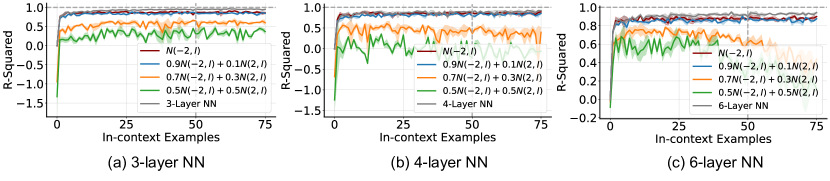
In this section, we conduct experiments to validate Objectives 1 and 2. We sample the input of feed-forward network $x\in\mathbb{R}^{d}$ from the Gaussian mixture distribution: $w_{1}N(-2,I_{d})+w_{2}N(2,I_{d})$, where $w_{1},w_{2}\in\mathbb{R}$. We consider three kinds of network $f:\mathbb{R}^{d}\rightarrow\mathbb{R}$, (i) 3-layer NN, (ii) 4-layer NN, and (iii) 6-layer NN. We generate the true output by $y=f(x)$. In our setting, we use $d=20$.

Model Architecture. The sole difference between ReLU-Transformer and $\mathop{\rm{Softmax}}$-Transformer is the activation function in the attention layer. Both models comprise 12 transformer blocks, each with 8 attention heads, and share the same hidden and MLP dimensions of 256.

Transformer Pretraining. We pretrain the ReLU-Transformer and $\mathop{\rm{Softmax}}$-Transformer based on the GPT-2 backbone. In our setting, we sample the pertaining data from $N(-2,I_{d})$, i.e., $w_{1}=1$ and $w_{2}=0$. Following the pre-training method in (Garg et al., 2022), we use the batch size as 64. To construct each sample in a batch, we use the following steps (take the generation for the $i$-th sample as an example):

  1. 1.

    Initialize the parameters in $f_{i}$ with a Gaussian distribution.

  2. 2.

    Generate $n$ queries $\left\{x_{i,j}\right\}_{j=1}^{n}$ (i.e., input of $f_{i}$) from the Gaussian mixture model $\omega_{1}N(-2,I)+\omega_{2}N(2,I)$. Here we take $n=51$.

  3. 3.

    For each query $x_{i,j}$, use $y_{i,j}=f_{i}(x_{i,j})$ to calculate the true output.

This generates a training sample for the transformer model with inputs

$\displaystyle\left[x_{i,1},y_{i,1},\cdots,x_{i,50},y_{i,50},x_{i,51}\right],$

and training target

$\displaystyle o_{i}=\left[y_{i,1},\cdots,y_{i,50},y_{i,51}\right].$

We use the MSE loss between prediction and true value of $o_{i}$. The pretraining process iterates for $500\mathrm{k}$ steps.

Testing Method. We generate samples similar to the pretraining process. The batch size is 64, and the number of batch is 100, i.e., we have 6400 samples totally. For each sample, we extend the value $n$ from 51 to 76 to learn the performance of in-context learning when the prompt length is longer than we used in pretraining. The input to the model becomes

$\displaystyle\left[x_{i,1},y_{i,1},\cdots,x_{i,75},y_{i,75},x_{i,76}\right].$

We assess performance using the mean R-squared value for all 6400 samples.

Baseline. We use the 3-layer, 4-layer, and 6-layer feed-forward neural networks as baselines by training them with in-context examples. Specially, given a testing sample (take the $i$-th sample as an example), which includes prompts $\left\{x_{i,j},y_{i,j}\right\}_{j=1}^{k-1}$ and a test query $x_{i,k}$. We use $\left\{x_{i,j},y_{i,j}\right\}_{j=1}^{k-1}$ to train the network with MSE loss for 100 epochs. We select the highest R-squared value from each epoch as the testing measure and calculate the average across all 6400 samples.

G.1.1 Performance of ReLU Transformer.

We use three different Gaussian mixture distribution $\omega_{1}N(-2,I)+\omega_{2}N(2,I)$ for the testing data: (i) $\omega_{1}=1,\omega_{2}=0$, (ii) $\omega_{1}=0.9,\omega_{2}=0.1$, (iii) $\omega_{1}=0.7,\omega_{2}=0.3$, (iv) $\omega_{1}=0.5,\omega_{2}=0.5$. Here, the distribution in the first setting matches the distribution in pretraining. We show the results in Figure 1.

Refer to caption
Figure 1: Performance of ICL in ReLU-Transformer: ICL learns 3-layer, 4-layer, and 6-layer NN and achieves R-squared values comparable to those from training with prompt samples. The results also show the ICL performance declines as the testing distribution diverges from the pretraining one.
G.1.2 Performance of Softmax Transformer.

We use three different Gaussian mixture distribution $\omega_{1}N(-2,I)+\omega_{2}N(2,I)$ for the testing data: (i) $\omega_{1}=1,\omega_{2}=0$, (ii) $\omega_{1}=0.9,\omega_{2}=0.1$, (iii) $\omega_{1}=0.7,\omega_{2}=0.3$, (iv) $\omega_{1}=0.5,\omega_{2}=0.5$. Here the distribution in the first setting matches the distribution in pretraining. We show the results in Figure 2.

Refer to caption
Figure 2: Performance of ICL in $\mathop{\rm{Softmax}}$-Transformer: ICL learns 3-layer, 4-layer, and 6-layer NN and achieves R-squared values comparable to those from training with prompt samples. The results also show the ICL performance declines as the testing distribution diverges from the pretraining one. Note that performance decreases when the prompt length exceeds the pretraining length (i.e., 50), a well-known issue (Dai et al., 2019; Anil et al., 2022). We believe this is due to the absolute positional encodings in GPT-2, as noted in (Zhang et al., 2023)

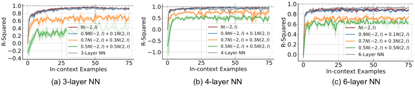
The results in Section G.1.1 and Section G.1.2 show that the performance of ICL in the transformer matches that of training $N$-layer networks, regardless of whether the prompt lengths are within or exceed those used in pretraining. Furthermore, the ICL performance declines as the testing distribution diverges from the pretraining one.

G.2 Experiments for Objective 3

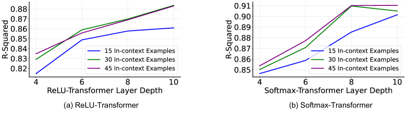
In this section, we conduct experiments to validate Objective 3. For these experiments, we use testing data identical to the pertaining data from $N(-2,I)$. We vary the number of layers in the transformer architecture, testing configurations with 4, 6, 8 and 10 layers. All other model hyperparameters and experimental details remain consistent with those described in Section G.1. We evaluate the ICL performance of both the ReLU-Transformer and the $\mathop{\rm{Softmax}}$-Transformer with 15, 30, and 45 in-context examples, as shown in Figure 3. The results show that a deeper transformer achieves better ICL performance, supporting the idea that scaling up the transformer enables it to perform more ICGD steps.

Refer to caption
Figure 3: Performance of ICL Across Varying Transformer Depths: We use the number of in-context examples as 15, 30, or 45 for both the ReLU-Transformer and the $\mathop{\rm{Softmax}}$-Transformer. The results show that a deeper transformer achieves better ICL performance, supporting the idea that scaling up the transformer enables it to perform more ICGD steps.

Appendix H Application: ICL for Diffusion Score Approximation

In this part, we give an important application of our work, i.e., learn the score function of diffusion models by the in-context learning of transformer models. We give the preliminaries about score matching generative diffusion models in Section H.1. Then, we give the analysis for ICL to approximate the diffusion score function in Section H.2.

H.1 Score Matching Generative Diffusion Models

Diffusion Model. Let $x_{0}\in\mathbb{R}^{d}$ be initial data following target data distribution $x_{0}\sim P_{0}$. In essence, a diffusion generative model consists of two stochastic process in $\mathbb{R}^{d}$:

  • A forward process gradually add noise to the initial data (e.g., images): $x_{0}\to x_{1}\to\cdots\to x_{T}$.

  • A backward process gradually remove noise from pure noise: $y_{T}\to y_{T-1}\to\cdots\to y_{0}$.

Importantly, the backward process is the reversed forward process, i.e., $y_{t}\stackrel{{\scriptstyle\mathrm{d}}}{{\approx}}x_{T-t}$ for $i\in 0,\ldots,T$.222$\stackrel{{\scriptstyle\mathrm{d}}}{{\approx}}$ denotes distributional equivalence. This allows the backward process to reconstruct the initial data from noise, and hence generative. To achieve this time-reversal, a diffusion model learns the reverse process by ensuring the backward conditional distributions mirror the forward ones. The most prevalent technique for aligning these conditional dynamics is through “score matching” — a strategy training a model to match score function, i.e., the gradients of the log marginal density of the forward process (Song et al., 2020b, a; Vincent, 2011). To be precise, let $P_{t},p_{t}(\cdot)$ denote the distribution function and destiny function of $x_{t}$. The score function is given by $\nabla\log p_{t}(\cdot)$. In this work, we focus on leveraging the in-context learning (ICL) capability of transformers to emulate the score-matching training process.

Score Matching Loss. We introduce the basic setting of score-matching as follows333Please also see Section B.1 and (Chen et al., 2024b; Chan, 2024; Yang et al., 2023) for overviews.. To estimate the score function, we use the following loss to train a score network $s_{W}(\cdot,t)$ with parameters $W$:

$\displaystyle\min_{W}\int_{T_{0}}^{T}\gamma(t)\mathbb{E}_{x_{t}\sim P_{t}}\left[\norm{s_{W}(x_{t},t)-\nabla\log p_{t}(x_{t})}_{2}^{2}\right]\differential t,\quad\text{where $\gamma(t)$ is a weight function,}$ (H.1)

and $T_{0}$ is a small value for stabilizing training and preventing the score function from diverging. In practice, as $\nabla\log p_{t}(\cdot)$ is unknown, we minimize the following equivalent loss (Vincent, 2011).

$\displaystyle\min_{W}\int_{T_{0}}^{T}\gamma(t)\mathbb{E}_{x_{0}\sim P_{0}}\left[\mathbb{E}_{x_{t}|x_{0}}\left[\norm{s_{W}(x_{t},t)-\nabla\log p(x_{t}|x_{0})}_{2}^{2}\right]\right]\differential t,$ (H.2)

where $p(x_{t}|x_{0})$ is distribution of $x_{t}$ conditioned on $x_{0}$.

H.2 ICL for Score Approximation

We first give the problem setup about the ICL for score approximation as the following:

Problem 3 (In-Context Learning (ICL) for Score Function $\nabla\log p_{t}(\cdot)$).

Consider the score function $\nabla\log p_{t}(\cdot)$ for any $t\geq 0$. Given a dataset $\mathcal{D}_{n}\coloneqq\left\{(x_{i},y_{i})\right\}_{i\in[n]}$, where $\left\{x_{i}\right\}_{i\in[n]}\subseteq\mathbb{R}^{d}$ and $y_{i}=\nabla\log p_{t_{i}}(x_{i})\subseteq\mathbb{R}^{d}$ ($t_{i}\geq 0$), and a test input $x_{n+1}$, the goal of “ICL for Score Function” is to find a transformer $\mathcal{T}$ to predict $y_{n+1}$ based on $x_{n+1}$ and the in-context dataset $\mathcal{D}_{n}$. In essence, the desired transformer $\mathcal{T}$ serves as the trained score network $s_{W}(\cdot,t)$.

To solve Problem 3, we follow two steps: (i) Approximate the diffusion score function $\nabla\log p_{t}(\cdot)$ with a multi-layer feed-forward network with ReLU activation functions under the given training dataset $\mathcal{D}_{n}$. (ii) Approximate the gradient descent used to train this network by the in-context learning of the Transformer until convergence, using the same training set $\mathcal{D}_{n}$ as the prompts of ICL.

For the first step, we follow the score approximation results based on a multi-layer feed-forward network with ReLU activation in (Chen et al., 2023), stated as next lemma.

Lemma 19 (Score Approximation by Feed-Forward Networks, Theorem 1 of (Chen et al., 2023)).

Given an approximation error $\epsilon>0$, for any initial data distribution $P_{0}$, there exist a multi-layer feed-forward network with ReLU activation, $f(w,x,t):\mathbb{R}^{D_{w}}\times\mathbb{R}^{d}\times\mathbb{R}\rightarrow\mathbb{R}^{d}$. Then for any $t\in[T_{0},T]$, we have $\norm{f(w,\cdot,t)-\nabla\log p_{t}(\cdot)}_{L^{2}(P_{t})}\leq\mathcal{O}(\epsilon)$.

With the approximation result, we reduce the Problem 3 to Problem 2, where the loss function is (H.1). Following Theorem 1, we show that the in-context learning of transformer models can approximate the score function of diffusion model.

References

  • Achiam et al. [2023] Josh Achiam, Steven Adler, Sandhini Agarwal, Lama Ahmad, Ilge Akkaya, Florencia Leoni Aleman, Diogo Almeida, Janko Altenschmidt, Sam Altman, Shyamal Anadkat, et al. Gpt-4 technical report. arXiv preprint arXiv:2303.08774, 2023.
  • Anil et al. [2022] Cem Anil, Yuhuai Wu, Anders Andreassen, Aitor Lewkowycz, Vedant Misra, Vinay Ramasesh, Ambrose Slone, Guy Gur-Ari, Ethan Dyer, and Behnam Neyshabur. Exploring length generalization in large language models. Advances in Neural Information Processing Systems, 35:38546–38556, 2022.
  • Bai et al. [2023] Yu Bai, Fan Chen, Huan Wang, Caiming Xiong, and Song Mei. Transformers as statisticians: Provable in-context learning with in-context algorithm selection. arXiv preprint arXiv:2306.04637, 2023.
  • Bi et al. [2024] Xiao Bi, Deli Chen, Guanting Chen, Shanhuang Chen, Damai Dai, Chengqi Deng, Honghui Ding, Kai Dong, Qiushi Du, Zhe Fu, et al. Deepseek llm: Scaling open-source language models with longtermism. arXiv preprint arXiv:2401.02954, 2024.
  • Bommasani et al. [2021] Rishi Bommasani, Drew A Hudson, Ehsan Adeli, Russ Altman, Simran Arora, Sydney von Arx, Michael S Bernstein, Jeannette Bohg, Antoine Bosselut, Emma Brunskill, et al. On the opportunities and risks of foundation models. arXiv preprint arXiv:2108.07258, 2021.
  • Brown [2020] Tom B Brown. Language models are few-shot learners. arXiv preprint arXiv:2005.14165, 2020.
  • Bubeck et al. [2023] Sébastien Bubeck, Varun Chandrasekaran, Ronen Eldan, Johannes Gehrke, Eric Horvitz, Ece Kamar, Peter Lee, Yin Tat Lee, Yuanzhi Li, Scott Lundberg, et al. Sparks of artificial general intelligence: Early experiments with gpt-4. arXiv preprint arXiv:2303.12712, 2023.
  • Chan [2024] Stanley H Chan. Tutorial on diffusion models for imaging and vision. arXiv preprint arXiv:2403.18103, 2024.
  • Chen et al. [2024a] Bo Chen, Xiaoyu Li, Yingyu Liang, Zhenmei Shi, and Zhao Song. Bypassing the exponential dependency: Looped transformers efficiently learn in-context by multi-step gradient descent. arXiv preprint arXiv:2410.11268, 2024a.
  • Chen et al. [2022] Mingda Chen, Jingfei Du, Ramakanth Pasunuru, Todor Mihaylov, Srini Iyer, Veselin Stoyanov, and Zornitsa Kozareva. Improving in-context few-shot learning via self-supervised training. arXiv preprint arXiv:2205.01703, 2022.
  • Chen et al. [2023] Minshuo Chen, Kaixuan Huang, Tuo Zhao, and Mengdi Wang. Score approximation, estimation and distribution recovery of diffusion models on low-dimensional data. In International Conference on Machine Learning, pages 4672–4712. PMLR, 2023.
  • Chen et al. [2024b] Minshuo Chen, Song Mei, Jianqing Fan, and Mengdi Wang. An overview of diffusion models: Applications, guided generation, statistical rates and optimization. arXiv preprint arXiv:2404.07771, 2024b.
  • Collins et al. [2024] Liam Collins, Advait Parulekar, Aryan Mokhtari, Sujay Sanghavi, and Sanjay Shakkottai. In-context learning with transformers: Softmax attention adapts to function lipschitzness. arXiv preprint arXiv:2402.11639, 2024.
  • Dai et al. [2022] Damai Dai, Yutao Sun, Li Dong, Yaru Hao, Shuming Ma, Zhifang Sui, and Furu Wei. Why can gpt learn in-context? language models implicitly perform gradient descent as meta-optimizers. arXiv preprint arXiv:2212.10559, 2022.
  • Dai et al. [2019] Zihang Dai, Zhilin Yang, Yiming Yang, Jaime Carbonell, Quoc V Le, and Ruslan Salakhutdinov. Transformer-xl: Attentive language models beyond a fixed-length context. arXiv preprint arXiv:1901.02860, 2019.
  • Garg et al. [2022] Shivam Garg, Dimitris Tsipras, Percy S Liang, and Gregory Valiant. What can transformers learn in-context? a case study of simple function classes. Advances in Neural Information Processing Systems, 35:30583–30598, 2022.
  • Gu et al. [2023] Yuxian Gu, Li Dong, Furu Wei, and Minlie Huang. Pre-training to learn in context. arXiv preprint arXiv:2305.09137, 2023.
  • Hu et al. [2024a] Jerry Yao-Chieh Hu, Wei-Po Wang, Ammar Gilani, Chenyang Li, Zhao Song, and Han Liu. Fundamental limits of prompt tuning transformers: Universality, capacity and efficiency. arXiv preprint, 2024a. To appear.
  • Hu et al. [2024b] Jerry Yao-Chieh Hu, Weimin Wu, Yi-Chen Lee, Yu-Chao Huang, Minshuo Chen, and Han Liu. On statistical rates of conditional diffusion transformer: Approximation and estimation. arXiv preprint, 2024b. To appear.
  • Jiang et al. [2024] Albert Q Jiang, Alexandre Sablayrolles, Antoine Roux, Arthur Mensch, Blanche Savary, Chris Bamford, Devendra Singh Chaplot, Diego de las Casas, Emma Bou Hanna, Florian Bressand, et al. Mixtral of experts. arXiv preprint arXiv:2401.04088, 2024.
  • Kajitsuka and Sato [2024] Tokio Kajitsuka and Issei Sato. Are transformers with one layer self-attention using low-rank weight matrices universal approximators? In The Twelfth International Conference on Learning Representations (ICLR), 2024.
  • Li et al. [2023] Shuai Li, Zhao Song, Yu Xia, Tong Yu, and Tianyi Zhou. The closeness of in-context learning and weight shifting for softmax regression. arXiv preprint arXiv:2304.13276, 2023.
  • Min et al. [2022] Sewon Min, Xinxi Lyu, Ari Holtzman, Mikel Artetxe, Mike Lewis, Hannaneh Hajishirzi, and Luke Zettlemoyer. Rethinking the role of demonstrations: What makes in-context learning work? In Proceedings of the 2022 Conference on Empirical Methods in Natural Language Processing, pages 11048–11064, 2022.
  • Panwar et al. [2023] Madhur Panwar, Kabir Ahuja, and Navin Goyal. In-context learning through the bayesian prism. arXiv preprint arXiv:2306.04891, 2023.
  • Radford et al. [2019] Alec Radford, Jeffrey Wu, Rewon Child, David Luan, Dario Amodei, Ilya Sutskever, et al. Language models are unsupervised multitask learners. OpenAI blog, 1(8):9, 2019.
  • Safran and Shamir [2017] Itay Safran and Ohad Shamir. Depth-width tradeoffs in approximating natural functions with neural networks. In International conference on machine learning, pages 2979–2987. PMLR, 2017.
  • Shi et al. [2023] Weijia Shi, Sewon Min, Maria Lomeli, Chunting Zhou, Margaret Li, Victoria Lin, Noah A Smith, Luke Zettlemoyer, Scott Yih, and Mike Lewis. In-context pretraining: Language modeling beyond document boundaries. arXiv preprint arXiv:2310.10638, 2023.
  • Shi et al. [2024] Zhenmei Shi, Junyi Wei, Zhuoyan Xu, and Yingyu Liang. Why larger language models do in-context learning differently? arXiv preprint arXiv:2405.19592, 2024.
  • Shin et al. [2022] Seongjin Shin, Sang-Woo Lee, Hwijeen Ahn, Sungdong Kim, HyoungSeok Kim, Boseop Kim, Kyunghyun Cho, Gichang Lee, Woomyoung Park, Jung-Woo Ha, et al. On the effect of pretraining corpora on in-context learning by a large-scale language model. arXiv preprint arXiv:2204.13509, 2022.
  • Song et al. [2020a] Yang Song, Sahaj Garg, Jiaxin Shi, and Stefano Ermon. Sliced score matching: A scalable approach to density and score estimation. In Uncertainty in Artificial Intelligence, pages 574–584. PMLR, 2020a.
  • Song et al. [2020b] Yang Song, Jascha Sohl-Dickstein, Diederik P Kingma, Abhishek Kumar, Stefano Ermon, and Ben Poole. Score-based generative modeling through stochastic differential equations. In International Conference on Learning Representations, 2020b.
  • Team et al. [2023] Gemini Team, Rohan Anil, Sebastian Borgeaud, Yonghui Wu, Jean-Baptiste Alayrac, Jiahui Yu, Radu Soricut, Johan Schalkwyk, Andrew M Dai, Anja Hauth, et al. Gemini: a family of highly capable multimodal models. arXiv preprint arXiv:2312.11805, 2023.
  • Touvron et al. [2023] Hugo Touvron, Thibaut Lavril, Gautier Izacard, Xavier Martinet, Marie-Anne Lachaux, Timothée Lacroix, Baptiste Rozière, Naman Goyal, Eric Hambro, Faisal Azhar, et al. Llama: Open and efficient foundation language models. arXiv preprint arXiv:2302.13971, 2023.
  • Vincent [2011] Pascal Vincent. A connection between score matching and denoising autoencoders. Neural computation, 23(7):1661–1674, 2011.
  • Von Oswald et al. [2023] Johannes Von Oswald, Eyvind Niklasson, Ettore Randazzo, João Sacramento, Alexander Mordvintsev, Andrey Zhmoginov, and Max Vladymyrov. Transformers learn in-context by gradient descent. In International Conference on Machine Learning, pages 35151–35174. PMLR, 2023.
  • Wang et al. [2024] Zhijie Wang, Bo Jiang, and Shuai Li. In-context learning on function classes unveiled for transformers. In Forty-first International Conference on Machine Learning, 2024.
  • Wei et al. [2023] Jerry Wei, Jason Wei, Yi Tay, Dustin Tran, Albert Webson, Yifeng Lu, Xinyun Chen, Hanxiao Liu, Da Huang, Denny Zhou, et al. Larger language models do in-context learning differently. arXiv preprint arXiv:2303.03846, 2023.
  • Wei et al. [2024] Jerry Wei, Jason Wei, Yi Tay, Dustin Tran, Albert Webson, Yifeng Lu, Xinyun Chen, Hanxiao Liu, Da Huang, Denny Zhou, and Tengyu Ma. Larger language models do in-context learning differently, 2024.
  • Wies et al. [2024] Noam Wies, Yoav Levine, and Amnon Shashua. The learnability of in-context learning. Advances in Neural Information Processing Systems, 36, 2024.
  • Xie et al. [2021] Sang Michael Xie, Aditi Raghunathan, Percy Liang, and Tengyu Ma. An explanation of in-context learning as implicit bayesian inference. arXiv preprint arXiv:2111.02080, 2021.
  • Xu et al. [2024] Zhuoyan Xu, Zhenmei Shi, and Yingyu Liang. Do large language models have compositional ability? an investigation into limitations and scalability. In ICLR 2024 Workshop on Mathematical and Empirical Understanding of Foundation Models, 2024.
  • Yang et al. [2023] Ling Yang, Zhilong Zhang, Yang Song, Shenda Hong, Runsheng Xu, Yue Zhao, Wentao Zhang, Bin Cui, and Ming-Hsuan Yang. Diffusion models: A comprehensive survey of methods and applications. ACM Computing Surveys, 56(4):1–39, 2023.
  • Yoo et al. [2022] Kang Min Yoo, Junyeob Kim, Hyuhng Joon Kim, Hyunsoo Cho, Hwiyeol Jo, Sang-Woo Lee, Sang-goo Lee, and Taeuk Kim. Ground-truth labels matter: A deeper look into input-label demonstrations. arXiv preprint arXiv:2205.12685, 2022.
  • Zhang et al. [2023] Ruiqi Zhang, Spencer Frei, and Peter L Bartlett. Trained transformers learn linear models in-context. arXiv preprint arXiv:2306.09927, 2023.
  • Zhang et al. [2022] Susan Zhang, Stephen Roller, Naman Goyal, Mikel Artetxe, Moya Chen, Shuohui Chen, Christopher Dewan, Mona Diab, Xian Li, Xi Victoria Lin, et al. Opt: Open pre-trained transformer language models. arXiv preprint arXiv:2205.01068, 2022.