:
\theoremsep
\jmlrvolume
\firstpageno1
\jmlryear2024
\jmlrworkshopSymmetry and Geometry in Neural Representations
On the Reconstruction of Training Data from Group Invariant Networks
Abstract
Reconstructing training data from trained neural networks is an active area of research with significant implications for privacy and explainability. Recent advances have demonstrated the feasibility of this process for several data types. However, reconstructing data from group-invariant neural networks poses distinct challenges that remain largely unexplored. This paper addresses this gap by first formulating the problem and discussing some of its basic properties. We then provide an experimental evaluation demonstrating that conventional reconstruction techniques are inadequate in this scenario. Specifically, we observe that the resulting data reconstructions gravitate toward symmetric inputs on which the group acts trivially, leading to poor-quality results. Finally, we propose two novel methods aiming to improve reconstruction in this setup and present promising preliminary experimental results. Our work sheds light on the complexities of reconstructing data from group invariant neural networks and offers potential avenues for future research in this domain.
keywords:
Group invariant neural networks, Dataset reconstruction, Privacy attacks1 Introduction
Recent works (Haim et al., 2022; Oz et al., 2024; Loo et al., 2023) have shown that it is possible to reconstruct training data from standard neural networks. However, the reconstruction from group invariant neural networks, such as networks applied to point clouds (Zaheer et al., 2017; Qi et al., 2017), graph data (Gilmer et al., 2017) or images with rotation and reflection symmetries (Cohen and Welling, 2016), remains largely unexplored.
Unlike the standard case explored in previous works, reconstructing data from group invariant models faces the unique challenge of multiple distinct inputs representing the same data point (namely, the orbit of a data point). This paper addresses the task of reconstructing data from group invariant networks, focusing on the limitations of conventional methods and proposing novel solutions. Our key contributions include:
-
1.
A formal definition of the reconstruction problem for invariant networks, accompanied by a discussion of its fundamental properties and invariance characteristics.
-
2.
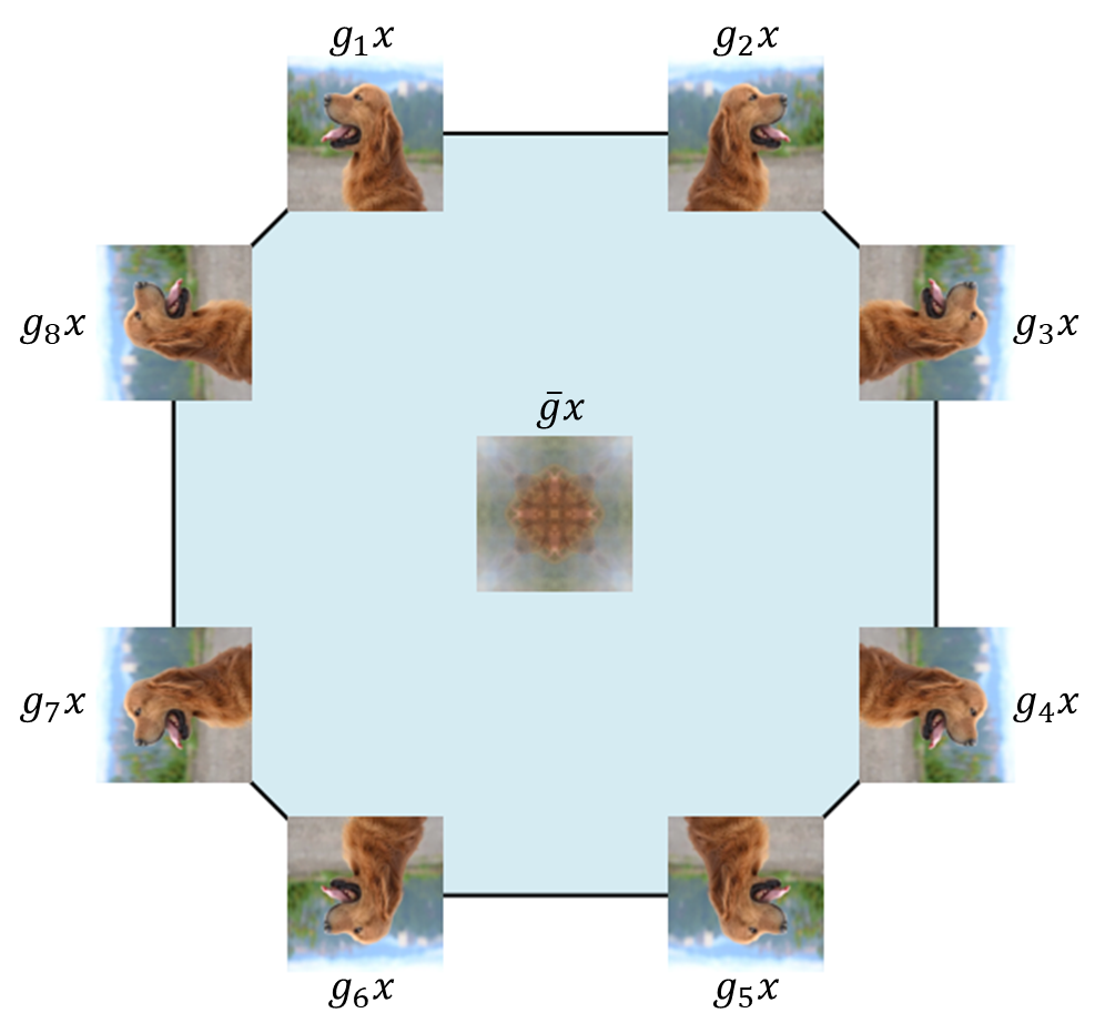
Empirical evidence demonstrating that conventional reconstruction methods converge to symmetric inputs (i.e., inputs on which the group acts trivially), producing low-quality reconstructions. The inset illustrates this phenomenon for : rather than recovering an element from a training example’s orbit, conventional methods often converge to the (symmetric) orbit average.
-
3.
Introduction of two novel techniques that enhance standard methods, enabling them to go beyond symmetric reconstructions with encouraging initial results.
-
4.
A discussion of potential future research directions.
2 Preliminaries
Invariance and equivariance. Let , be group representations of a finite group . We denote as the orbit of a vector under the group action and as its stabilizer group. The orbitope of a point (Sanyal et al. (2011)) is defined as the convex hull of as illustrated in \figurereffig: orbitopes. We denote the vectors on which the group acts trivially as , formally . The projection of a vector on , denoted as , is the average of its orbit, . A function is -invariant if for any and a function is -equivariant if for any . For simplicity, we denote .
Data Reconstruction. There are several methods to reconstruct training data from trained neural networks , where is the network’s input, and is a vectorization of its parameters. Here, we focus on two methods: (1) Activation Maximization (AM) (Fredrikson et al., 2015; Yang et al., 2019), where the goal is to look for the input, which maximizes the model output for the desired target class. Namely, the objective for class is defined as . (2) KKT-based reconstruction (Haim et al., 2022; Buzaglo et al., 2023). This method uses the implicit bias of homogeneous neural networks trained with gradient methods toward margin maximization. Here, the following objective is optimized: , (The denote the labels.). For a detailed description of the reconstruction methods, see Appendix B.
vspace-10pt
3 Reconstruction from Invariant networks
3.1 Problem definition
Let be a training dataset and let is an orthogonal representation of a finite group . Let be a pre-trained -invariant neural network with weights . We aim to find a set of reconstructions such that is the closest set to with respect to some evaluation metric.
Evaluation under group symmetries. Since the reconstruction of any element from the orbit is equally valid, the evaluation metric for invariant data reconstruction problems should be invariant to these group symmetries to ensure a fair assessment of model performance. This can be done, for example, by defining the distance between a reconstruction and a training example using the following metric . Note that invariant metrics may be computationally challenging, e.g. when the input is a graph.
Applying AM and KKT to the invariant case. In most cases the training of (homogeneous) invariant neural networks is conducted in a way that the conditions of both methods (AM and KKT-based) are met, so we can apply them to the invariant case.
3.2 Challenges and theoretical observations
Here we present basic theoretical findings and challenges in reconstructing data from invariant models, applicable to any orthogonal representation of a finite group. Full proofs are in the appendix.
(1) Multiple equivalent solutions. When reconstructing data from invariant models, a critical factor to consider is that each training sample can have multiple equivalent representations. These representations form what is known as an orbit under the group action.
Proposition 3.1.
If the model is -invariant then the objective functions of the methods mentioned in \sectionrefsec: Preliminaries are -invariant. Formally,
| (1) |
(2) Optimizing invariant reconstruction objectives using GD. As invariant reconstruction objectives have multiple optima, both initialization and optimization methods are crucial in determining the final solution. The following proposition sheds light on GD’s behavior in this context:
Proposition 3.2.
If the reconstruction objective function is -invariant function then: (i) the GD step is G-equivariant function of ; and (ii)
First, the above part (i) implies that GD is an equivariant function of the initialization, as it is a composition of equivariant functions (GD iterations). Therefore, the initialization determines which element the method converges to. Moreover, it implies that if we use invariant distribution for the initialization ( is a -invariant function) the algorithm induces an invariant distribution over the reconstructions. Moreover, the nesting of the stabilizers mentioned in part (ii) of Proposition 3.2 indicates that as optimization progresses, the stabilizers of the iterates may become more restrictive, thereby narrowing the exploration of the solution space. As we will see in the following sections, we believe that this property plays a significant role in the dynamics of optimization and can influence the final outcomes.
3.3 Ineffectiveness of standard methods in Invariant Reconstruction
This subsection presents experimental evidence demonstrating the ineffectiveness of AM and KKT-based methods in solving the invariant reconstruction problem. The full experimental results and description are on the appendix.
Setup and evaluation. We focus on the reconstruction of image data from invariant models of different groups of reflections and rotations (see \sectionrefappen: Experimental setting). To evaluate the results we used DSSIM proposed in Baker et al. (2023) for measuring differences between images (high DSSIM implies high structural dissimilarity).To ensure the invariance of our metric, we match reconstructions to training samples across all group transformations.
Results. As illustrated in Figures 4 and 4, the optimization often converges to invariant reconstructions, resulting in a significant loss of information and low-quality reconstructions. Moreover, our observations reveal that many reconstructions lie on the convex hull of sample orbits, or orbitopes. To understand the distribution of reconstructions on the orbitopes we sampled various points on the ground truth orbitopes and identified the nearest neighbors for each reconstruction. as depicted in Figure LABEL:fig:dssim_kkt the observed distribution aligns with our predictions in Section 3.2: the reconstructions are concentrated around the group average that lies in with the largest possible stabilizer. Notably, the KKT-based method outperforms activation maximization, as shown in Figure LABEL:fig:_dssim. Furthermore, we observe that increasing either the group size or the training set size leads to poorer results.
4 Symmetry-aware reconstruction
We propose two methods to improve reconstruction: mitigating GD’s bias towards symmetry and imposing meaningful input space priors.
Symmetry-Aware Memory-Enhanced Gradient Descent (SAME-GD). Empirically, we tend to converge to points with nontrivial stabilizers, in particular to points on or close to . We suggest aggregating the current query point with previous points in the optimization trajectory in a way that breaks the nesting property proved in Proposition 3.2. For simplicity, we used convex aggregation in the form of , see \algorithmrefalg:sam.
Incorporating Deep Image Prior (DIP). As proposed in Ulyanov et al. (2020), convolutional neural networks can be used as an implicit prior when it comes to inverse problems. We propose to use the same objective functions of the existing methods, but parameterizing the reconstruction variables as the output of a randomly initialized CNN instead of optimizing them directly. The motivation is that the natural image prior could potentially break the symmetry and enhance the quality of the reconstructions.
Preliminary experimental results. We investigated the reconstruction abilities of the proposed methods under different configurations as listed on \tablereftable: dssim. We extended our experimental results to include CIFAR-10 images, with binary labels indicating animals and vehicles. SAME-GD and DIP, when combined with the KKT objective, yield notably improved reconstructions. These methods show a reduced tendency to converge to group averages, thus preserving more meaningful data characteristics. Particularly noteworthy is the KKT with DIP approach (Figure LABEL:fig:_results), which excels in producing piece-wise smooth asymmetric reconstructions by exploiting the implicit prior induced by DIP.
fig: results
AM
 KKT
KKT
 KKT + SAME-GD
 KKT + DIP

| Dataset | Group size | Train set size | AM | KKT | KKT + SAME-GD | KKT + DIP |
|---|---|---|---|---|---|---|
| MNIST | 2 | 50 | ||||
| MNIST | 2 | 100 | ||||
| CIFAR-10 | 2 | 50 | – | |||
| CIFAR-10 | 2 | 100 | – | |||
| MNIST | 8 | 50 | ||||
| MNIST | 8 | 100 |
Discussion. Our work highlights the challenges in reconstructing training data from group-invariant neural networks. The theoretical and experimental foundations laid here raise questions about the behavior of reconstruction methods applied to these networks. Although we provide some insights and novel approaches, It is still unclear why standard reconstruction methods fail for invariant models. There are many future directions to be explored, some of them are discussed in more details in Appendix G.
HM is the Robert J. Shillman Fellow, and is supported by the Israel Science Foundation through a personal grant (ISF 264/23) and an equipment grant (ISF 532/23). We would like to thank Yam Eitan for his valuable contribution to this project.
References
- Baker et al. (2023) Allison H. Baker, Alexander Pinard, and Dorit M. Hammerling. Dssim: a structural similarity index for floating-point data, 2023. URL https://arxiv.org/abs/2202.02616.
- Buzaglo et al. (2023) Gon Buzaglo, Niv Haim, Gilad Yehudai, Gal Vardi, Yakir Oz, Yaniv Nikankin, and Michal Irani. Deconstructing data reconstruction: Multiclass, weight decay and general losses. In Advances in Neural Information Processing Systems, volume 36, pages 51515–51535, 2023.
- Cohen and Welling (2016) Taco Cohen and Max Welling. Group equivariant convolutional networks. In International conference on machine learning, pages 2990–2999. PMLR, 2016.
- Fredrikson et al. (2015) Matt Fredrikson, Somesh Jha, and Thomas Ristenpart. Model inversion attacks that exploit confidence information and basic countermeasures. In Proceedings of the 22nd ACM SIGSAC conference on computer and communications security, pages 1322–1333, 2015.
- Geiping et al. (2020) Jonas Geiping, Hartmut Bauermeister, Hannah Dröge, and Michael Moeller. Inverting gradients-how easy is it to break privacy in federated learning? Advances in Neural Information Processing Systems, 33:16937–16947, 2020.
- Gilmer et al. (2017) Justin Gilmer, Samuel S Schoenholz, Patrick F Riley, Oriol Vinyals, and George E Dahl. Neural message passing for quantum chemistry. In International conference on machine learning, pages 1263–1272. PMLR, 2017.
- Haim et al. (2022) Niv Haim, Gal Vardi, Gilad Yehudai, Ohad Shamir, and Michal Irani. Reconstructing training data from trained neural networks. Advances in Neural Information Processing Systems, 35:22911–22924, 2022.
- Hitaj et al. (2017) Briland Hitaj, Giuseppe Ateniese, and Fernando Perez-Cruz. Deep models under the gan: information leakage from collaborative deep learning. In Proceedings of the 2017 ACM SIGSAC conference on computer and communications security, pages 603–618, 2017.
- Huang et al. (2021) Yangsibo Huang, Samyak Gupta, Zhao Song, Kai Li, and Sanjeev Arora. Evaluating gradient inversion attacks and defenses in federated learning. Advances in Neural Information Processing Systems, 34:7232–7241, 2021.
- Ji and Telgarsky (2020) Ziwei Ji and Matus Telgarsky. Directional convergence and alignment in deep learning. In Advances in Neural Information Processing Systems (NeurIPS), 2020.
- Loo et al. (2023) Noel Loo, Ramin Hasani, Mathias Lechner, and Daniela Rus. Dataset distillation fixes dataset reconstruction attacks. arXiv preprint arXiv:2302.01428, 2023.
- Lyu and Li (2020) Kaifeng Lyu and Jian Li. Gradient descent maximizes the margin of homogeneous neural networks. In International Conference on Learning Representations (ICLR), 2020.
- Oz et al. (2024) Yakir Oz, Gilad Yehudai, Gal Vardi, Itai Antebi, Michal Irani, and Niv Haim. Reconstructing training data from real world models trained with transfer learning. arXiv preprint arXiv:2407.15845, 2024.
- Qi et al. (2017) Charles R Qi, Hao Su, Kaichun Mo, and Leonidas J Guibas. Pointnet: Deep learning on point sets for 3d classification and segmentation. In Proceedings of the IEEE conference on computer vision and pattern recognition, pages 652–660, 2017.
- Sanyal et al. (2011) Raman Sanyal, Frank Sottile, and Bernd Sturmfels. Orbitopes. Mathematika, 57(2):275–314, June 2011. ISSN 2041-7942. 10.1112/s002557931100132x. URL http://dx.doi.org/10.1112/S002557931100132X.
- Ulyanov et al. (2020) Dmitry Ulyanov, Andrea Vedaldi, and Victor Lempitsky. Deep image prior. International Journal of Computer Vision, 128(7):1867–1888, March 2020. ISSN 1573-1405. 10.1007/s11263-020-01303-4. URL http://dx.doi.org/10.1007/s11263-020-01303-4.
- Wu et al. (2021) Bang Wu, Xiangwen Yang, Shirui Pan, and Xingliang Yuan. Adapting membership inference attacks to gnn for graph classification: Approaches and implications, 2021.
- Yang et al. (2019) Ziqi Yang, Jiyi Zhang, Ee-Chien Chang, and Zhenkai Liang. Neural network inversion in adversarial setting via background knowledge alignment. In Proceedings of the 2019 ACM SIGSAC Conference on Computer and Communications Security, pages 225–240, 2019.
- Zaheer et al. (2017) Manzil Zaheer, Satwik Kottur, Siamak Ravanbakhsh, Barnabas Poczos, Russ R Salakhutdinov, and Alexander J Smola. Deep sets. Advances in neural information processing systems, 30, 2017.
- Zhang et al. (2021) Zaixi Zhang, Qi Liu, Zhenya Huang, Hao Wang, Chengqiang Lu, Chuanren Liu, and Enhong Chen. Graphmi: Extracting private graph data from graph neural networks, 2021.
- Zhu et al. (2019) Ligeng Zhu, Zhijian Liu, and Song Han. Deep leakage from gradients. Advances in Neural Information Processing Systems, 32, 2019.
Appendix A Previous work
Several methods have been developed to reconstruct training samples from neural networks under different settings. Activation-maximization attacks Fredrikson et al. (2015); Yang et al. (2019) optimize the target output class over the input. Another method is reconstruction in a federated learning setup Zhu et al. (2019); Hitaj et al. (2017); Geiping et al. (2020); Huang et al. (2021) where the attacker is assumed to have knowledge of the sample’s gradient. Several works use the implicit bias of neural networks towards margin maximization Lyu and Li (2020); Ji and Telgarsky (2020) to devise reconstruction losses, and thus reconstruct samples that are on the margin Haim et al. (2022); Buzaglo et al. (2023); Loo et al. (2023); Oz et al. (2024). Some prior studies have explored reconstructing graph structures from trained networks. The majority of existing research has concentrated on single-graph learning scenarios. In these cases, known node feature matrices effectively break symmetries, which simplifies the problem Zhang et al. (2021); Wu et al. (2021).
Appendix B Current reconstruction methods
This is elaboration of \sectionrefsec:Data Reconstruction in the main text. There are several methods to reconstruct training data from trained neural networks. In this work we focused on two methods which allow data reconstruction in a general setting with minimal assumptions on the model’s architecture.
Activation-Maximization (AM). We are given a trained multi-class classifier with classes. The predicted class of the classifier is defined as , namely, the class with the maximal output. In this reconstruction method, to reconstruct a sample in class , we randomly initialize an input and maximize the loss objective . This is done by applying a first-order optimization method such as (Gradient Descent) GD.
KKT-based reconstruction. Lyu and Li (2020); Ji and Telgarsky (2020) show that given a homogeneous111A function is homogeneous if for every we have neural network , trained with gradient flow using an exponentially tailed loss (e.g., binary cross entropy) on a binary classification dataset , its parameters converge to a KKT point of the following margin maximization problem
| (2) |
In particular, the KKT stationary condition is satisfied, namely there exist for such that . In Haim et al. (2022) the authors use the stationary condition to construct an objective that reconstructs the training data given the trained weights . Namely, they propose optimizing the following loss objective
| (3) |
where , the number of reconstruction candidates is chosen to be . This optimization problem in practice is solved by GD or similar optimization methods.
Appendix C Proof of proposition 3.1
The activation maximization objective function uses the model output directly. Since the model is invariant it is trivially implying that the objective loss is also invariant. As the KKT based method involves first-order derivatives we would start by proving the following lemma:
Lemma C.1.
Let be -invariant function w.r.t . Assume has a partial gradient by at . Then also has partial gradient by at . Moreover,
Proof C.2.
Denote to be the standard basis of . f is -invariant, therefore ,
| (4) |
Since it is given the limit of exists for the left side of the equation then the limit of the right side also exists and is equal to it. If we take the limit of both side, by definition we get:
| (5) |
In other words is -invariant. As the trained model is invariant, we can say that is also invariant and therefore the objective loss in the KKT based method is also invariant.
Appendix D Proof of proposition 3.2
We prove here the extended version of Proposition 3.2.
Proposition D.1.
Let be -invariant function w.r.t . Consider the following optimization problem
| (6) |
solved by the following iterates of GD with some learning rates
| (7) |
Then
-
1.
The gradient step is G-equivariant function of .
-
2.
We first start by addressing the equivariance of the gradient by .
Lemma D.2.
Let be -invariant function w.r.t and assume is an orthogonal matrix for all . If is derivable by at then is also derivable by at .
Moreover, .
Proof D.3.
For convenience, we would write instead of
By definition, for any direction ,
| (8) |
Where is the directional derivative of f at .
is -invariant, therefore:
| (9) | |||
| (10) | |||
| (11) | |||
| (12) |
On one hand,
| (13) |
On the other hand is orthogonal, then
| (14) | |||
| (15) | |||
| (16) |
Therefore,
| (18) |
In other words is -equivariant.
is -invariant, then by \lemmareflemma: equivariant gradient, for every and for any :
| (19) |
Therefore the gradient step is -equivariant.
if , then by definition Therefore:
| (20) | |||
| (21) | |||
| (22) | |||
| (23) | |||
| (24) |
Therefore
Appendix E Experimental setting
Setting. We focus on image data and considered 4 groups for our experiments - the trivial group, group of 2 elements acting as horizontal reflection, the group of 4 elements acting as horizontal and vertical reflection (Klein four-group), and the Dihedral group (rotations and reflections). To construct the invariant model we used a ReLU neural network with two hidden layers of width 1000 each and applied symmetrization 222 symmetrization is a common practice to project functions on the invariant function space using Reynolds operator . Initially we trained the models on MNIST images with binary labels for odd or even digits. For each group we trained a neural network with different training set sizes for 100K epochs. All training ended with training error and accuracy. For each method and configuration, we ran 5 experiments of reconstruction with different seeds and candidates (500 per class).
fig: dssim
\subfigure[KKT]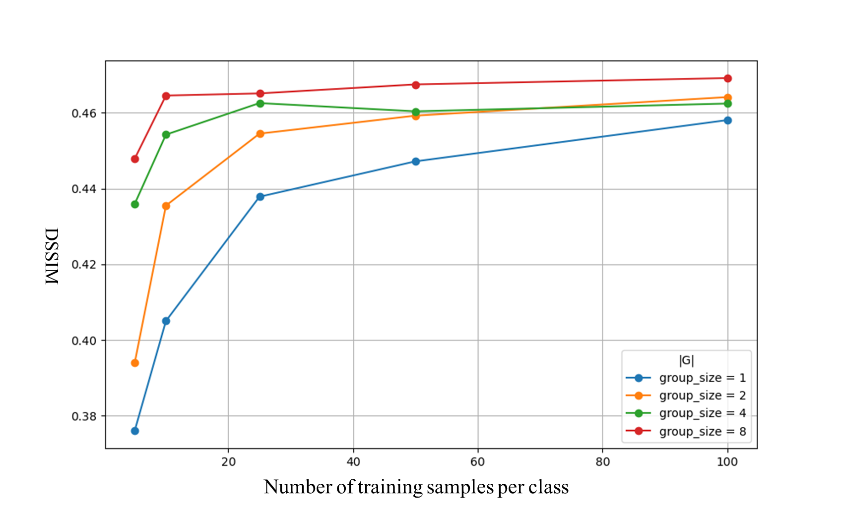 \subfigure[AM]
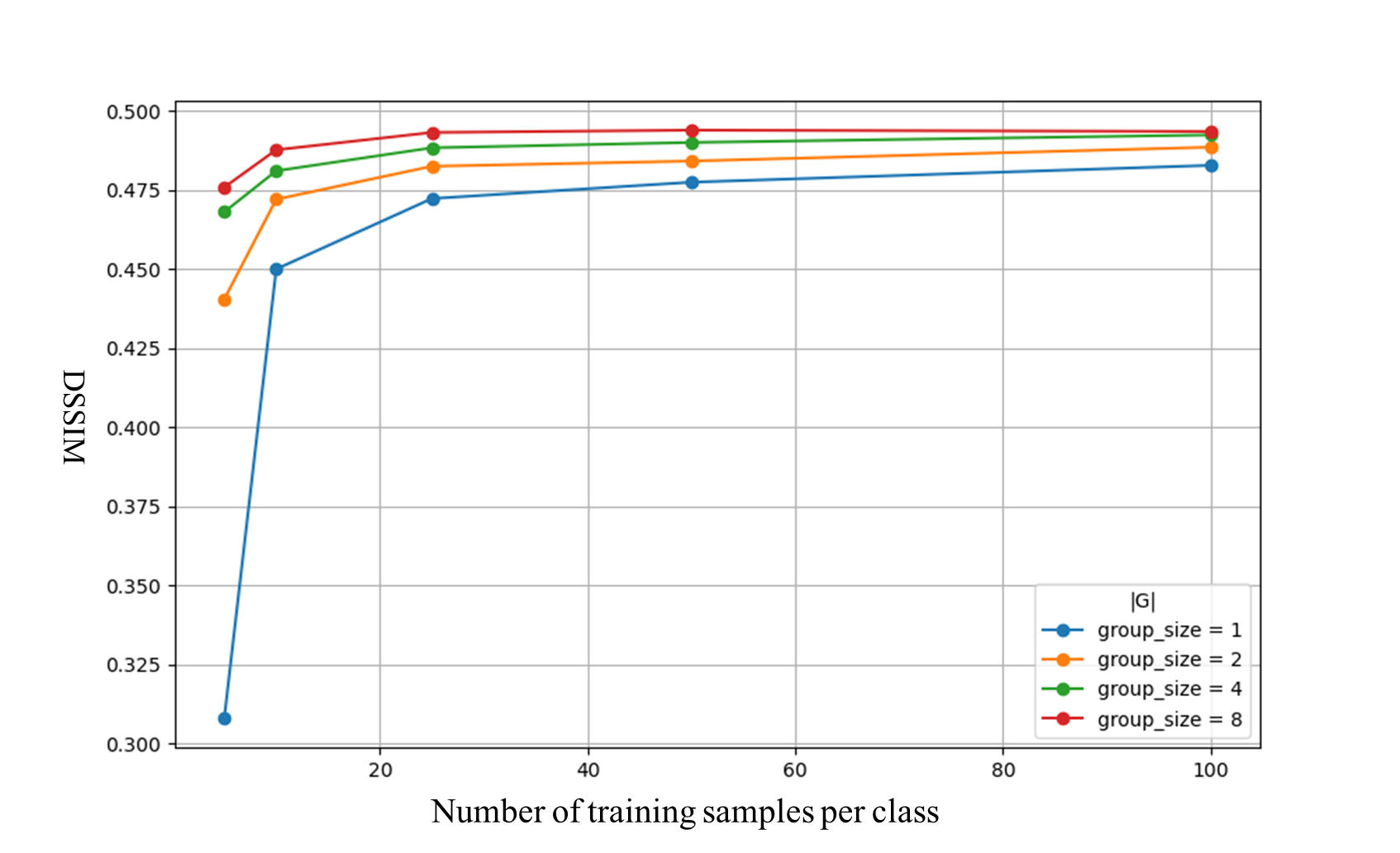
fig: results full
\subfigure[Activation Maximization]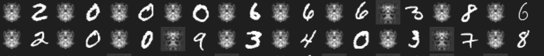
\subfigure[Vanilla KKT]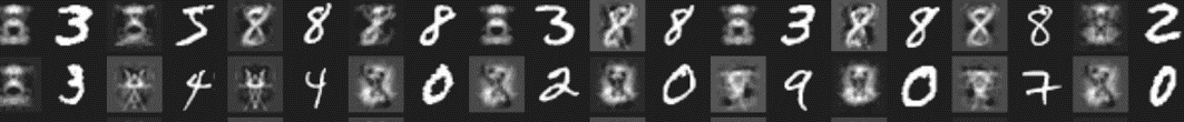
\subfigure[KKT with SAME-GD]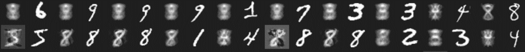
\subfigure[KKT with Deep Image Prior]
fig:dssim kkt
\subfigure[]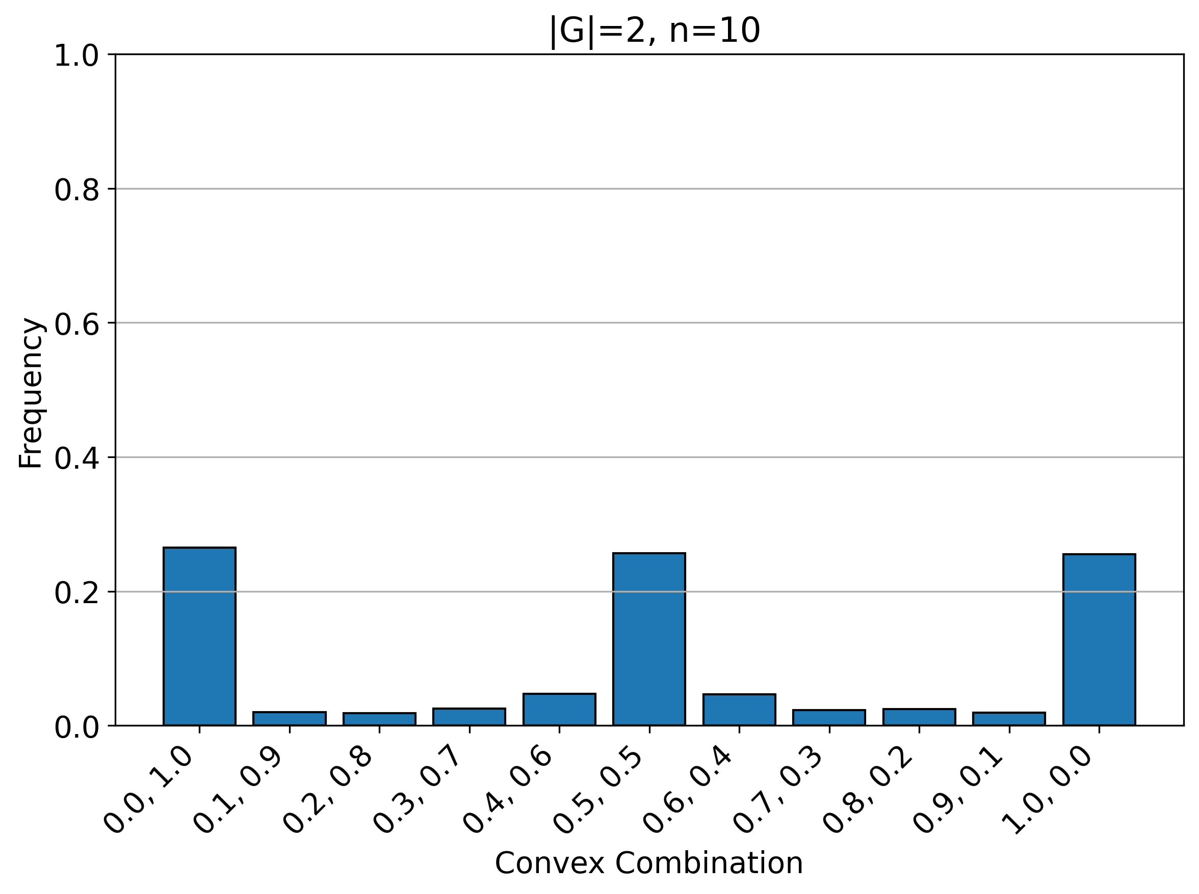 \subfigure[]
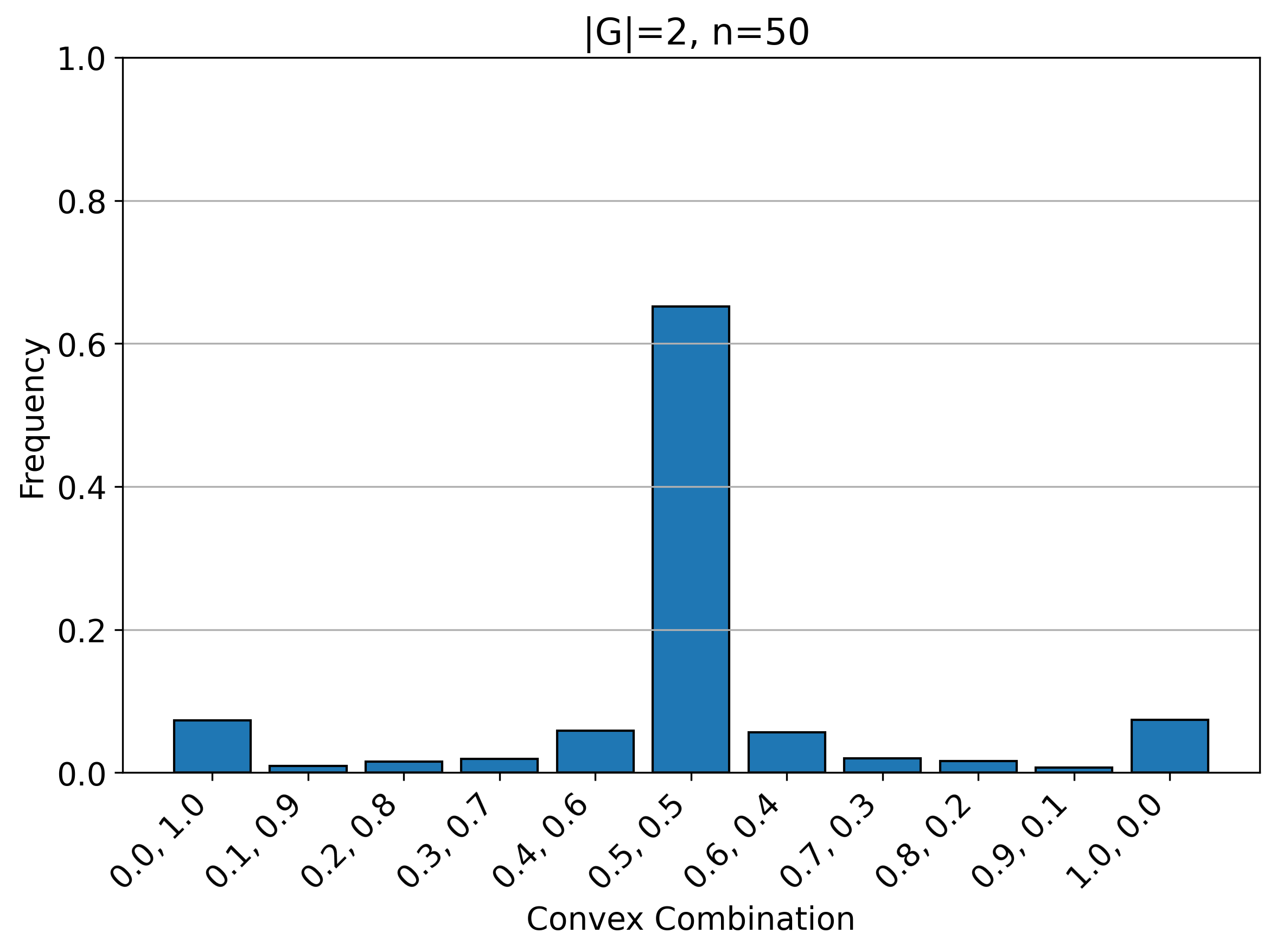 \subfigure[]
\subfigure[]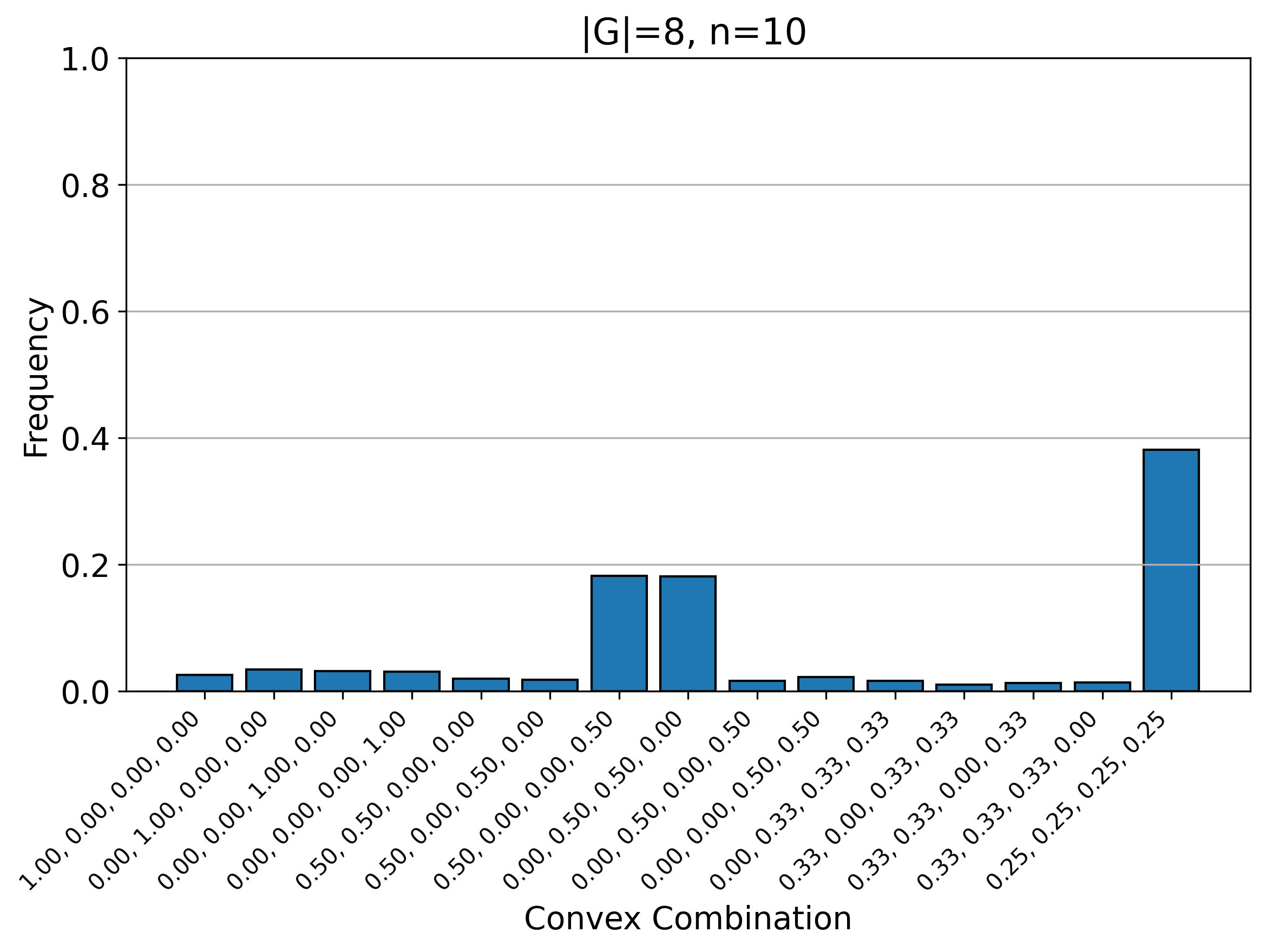 \subfigure[]
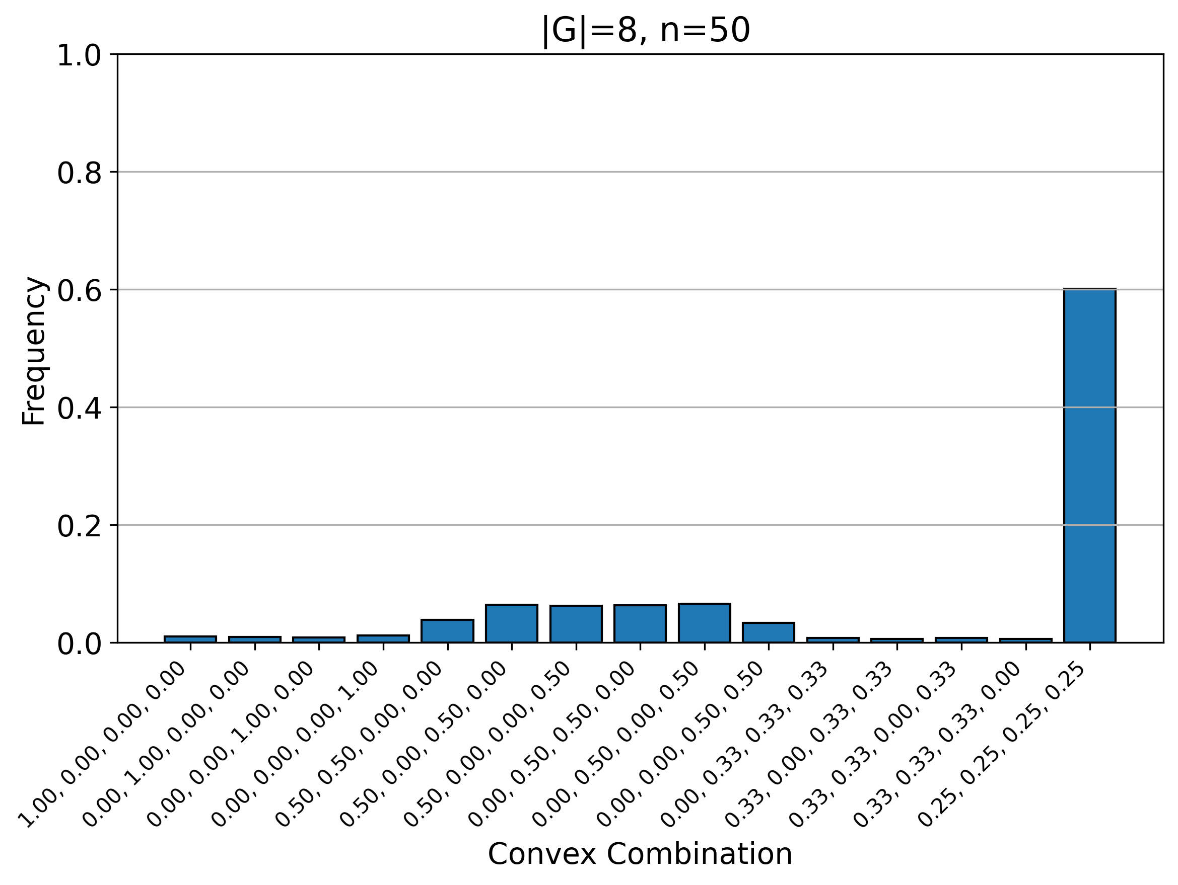 \subfigure[]
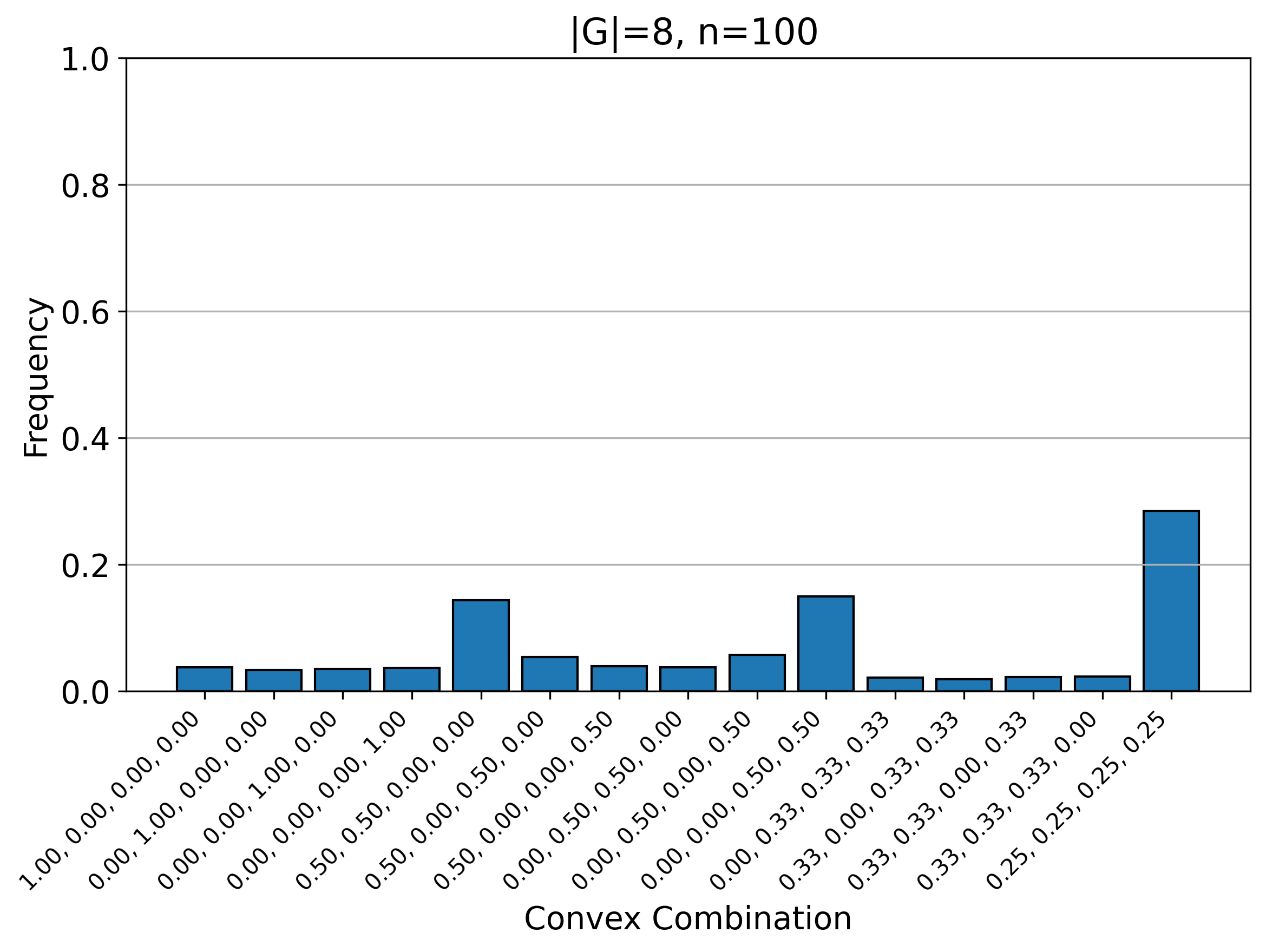
Appendix F SAME-GD
Appendix G Discussion and future directions
In this section we discuss in details some challenges and future directions that arise from this work:
-
•
Our work focuses on relatively small groups, containing at most elements, which contain only rotation and reflection transformations. It would be interesting to further study reconstruction from models that are invariant to much larger groups.
-
•
Our results indicate that reconstructions from invariant models lie close to the orbitope, mostly to the average over group elements. This finding only scratches the surface regarding how the reconstructions are distributed inside the orbitope, which may be effected by different factors such as initialization, architecture of the network, and structure of the group.
-
•
We propose several methods to guide the reconstructions towards specific elements in the group, and thus to reconstruct the actual training samples (up to group action). However, it is not clear how well these methods generalize to larger datasets or larger groups. It will also be interesting to find new methods for this task, for example methods that take advantage of the geometrical properties of the orbitope, and may push the reconstructions towards extreme points of the orbitope.
-
•
Our work focuses on image datasets, namely MNIST and CIFAR. It would be interesting to use these methods to reconstruct training samples from different data modalities, such as graphs or point clouds.
-
•
In this work the models are constructed to be invariant using symmetrization of the feed-forward model. There are other methods to construct invariant networks, such as parameter sharing-based techniques, and it would be interesting to study data reconstruction attacks on such networks.